Improved Online Contention Resolution for Matchings and Applications to the Gig Economy

Abstract

Motivated by applications in the gig economy, we study approximation algorithms for a sequential pricing problem. The input is a bipartite graph $G=(I,J,E)$ between individuals $I$ and jobs $J$. The platform has a value of $v_{j}$ for matching job $j$ to an individual worker. In order to find a matching, the platform can consider the edges $(ij)\in E$ in any order and make a one-time take-it-or-leave-it offer of a price $\pi_{ij}=w$ of its choosing to $i$ for completing $j$. The worker accepts the offer with a known probability $p_{ijw}$; in this case the job and the worker are irrevocably matched. What is the best way to make offers to maximize revenue and/or social welfare?

The optimal algorithm is known to be NP-hard to compute (even if there is only a single job). With this in mind, we design efficient approximations to the optimal policy via a new Random-Order Online Contention Resolution Scheme (RO-OCRS) for matching. Our main result is a 0.456-balanced RO-OCRS in bipartite graphs and a 0.45-balanced RO-OCRS in general graphs. These algorithms improve on the recent bound of $\frac{1}{2}(1-\texttt{e}^{-2})\approx 0.432$ of [BGMS21], and improve on the best known lower bounds for the correlation gap of matching, despite applying to a significantly more restrictive setting. As a consequence of our OCRS results, we obtain a $0.456$-approximate algorithm for the sequential pricing problem. We further extend our results to settings where workers can only be contacted a limited number of times, and show how to achieve improved results for this problem, via improved algorithms for the well-studied stochastic probing problem.

1 Introduction

Online gig platforms form a large and growing section of the economy. Gallup estimates that 36% of U.S. workers participate in the “gig economy” through either their primary or secondary jobs. This includes multiple types of alternative work arrangements from temp workers and contract nurses to millions of online platform workers (for platforms like DoorDash, Uber or TaskRabbit) providing rides, shopping, and delivery services.

One of the salient features of these app-based online platforms is that they pair workers with tasks in real-time. As a result of that, and because of interface limitations of mobile apps, pricing the tasks and matching them to workers cannot be done in one shot. Instead, platforms usually find matches for tasks by sending a take-it-or-leave-it offer through the app to the workers, detailing the task description and how much they will be paid, with a short window to decide. If one worker declines the offer, the job will be sent to another, possibly with a different price. Motivated by this, we consider the following problem abstraction.

The Sequential Pricing Problem.

The input is a bipartite graph $G=(I,J,E)$ with vertices on one side corresponding to the available individuals (workers) $I$ and jobs $J$. The platform can consider the edges in $E$ in any order; when considering edge $(ij)$, it makes a one-time take-it-or-leave-it offer of price $\pi_{ij}=w$ to worker $i$ for completing job $j$. The worker accepts with a (known) probability $p_{ijw}=p_{ew}$. In this case, the worker and job are irrevocably matched. For $A$ the set of matched jobs, and $\mu$ the edges these jobs are matched along, the platform’s revenue is $\sum_{j\in A}v_{j}-\sum_{(ij)\in\mu}\pi_{ij}$, where $v_{j}$ is the value of completing job $j\in J$.

We assume that the platform learns the probability that workers accept a job at a certain price through multiple interactions with them. We further assume that due to the size of the market, this learning is robust to strategic behavior of the workers and we therefore ignore such issues.

In our setting, the set of jobs and workers is fixed and known a priori. Even though that is rarely the case in practice, in many applications of interest the underlying network of between jobs and workers changes slowly. For example, in applications like pet sitting or grocery shopping, the tasks are often scheduled in advance. In the case of food delivery, there is usually a 20-30 minute lag between the time the requests are made and the jobs are available, so it is practical to implement our sequential pricing mechanisms over a shorter planning horizon.

In most settings, it is undesirable to overwhelm workers with too many queries. Therefore, we also consider the following generalization of our problem, borrowing the term patience from the literature on stochastic probing problems (see Section 1.4).

The Sequential Pricing Problem with Patience.

The setting is the same as above, but each worker $i$ has an associated patience $\ell_{i}\in\mathbb{Z}_{\geq 0}$ and we can only offer prices along at most $\ell_{i}$ edges incident on $i$.

It is not hard to see that the above sequential pricing problem is NP-hard even without patience constraints. In fact, using the reduction of Xiao et al. [XLH20], one can show that this is the case already when the number of workers is one.

With this challenge in mind, our goal is to design efficient pricing policies giving approximations to the revenue achievable by the optimum sequential pricing algorithm. We briefly note that while in many online stochastic matching problems, the goal is to achieve a constant-factor approximation to the optimum offline algorithm, such a result is impossible in our setting.

Our Approach: Reducing to (and Improving) Contention Resolution Schemes.

Our approach for designing efficient approximate sequential pricing algorithms is to first solve a natural linear programming (LP) relaxation, with variables $\{y_{ijw}\}$ representing the probability we offer price $w$ for worker $i$ to complete task $j$. We then round this LP in a (self-imposed) random-order online fashion. This gives a common algorithmic framework for sequential pricing with and without patience constraints. We show that the analysis of instantiations of our algorithm can be seen as a reduction to random-order online algorithms for two well-studied problem in the literature: (i) online contention resolution schemes (OCRS), and (ii) stochastic OCRS (closely related to stochastic probing). More generally, we show that any chosen-order contention resolution schemes for matching result in improved bounds for our problems.

Our quantitative results follow precisely from improved algorithms for these well-studied contention resolution scheme questions, which we now introduce.

1.1 Background: Contention Resolution Schemes

When rounding a solution to some LP relaxation of some constrained problem, the most natural approach is to independently round its decision variables. For example, consider the following well-studied fractional relaxation of matching constraints:

$$\mathcal{P}(G):=\left\{x\in\mathbb{R}^{E}_{\geq 0}\,\,\Bigg{|}\,\sum_{e\ni v}x_{e}\leq 1\quad\forall v\in V\right\}.$$ (1)

Let $\vec{x}\in\mathcal{P}(G)$ be a fractional solution to a matching problem with some linear objective $\vec{w}$. Rounding each edge $e$ independently will result in a random subset $R(x)\subseteq E$ of expected objective value equal to that of $\vec{w}\cdot\vec{x}$. Unfortunately, this set $R(x)$ will most likely not form an integral matching. How much smaller (in expectation) can the highest-valued matching in $R(x)$ be compared to $\vec{w}\cdot\vec{x}$? This is precisely the correlation gap of $\mathcal{P}(G)$, introduced in the context of stochastic optimization problems more generally in [ADSY12].

When rounding a point $\vec{x}\in\mathcal{P}(G)$ (and more generally in a polytope containing the convex hull of some constraint set), especially in constrained computational settings, to obtain a feasible integral solution, one must in some sense resolve contention between rounded edges (elements). This motivates the definition of contention resolution schemes (CRS), introduced by [CVZ14], and later extended to online settings by [FSZ16, AW18, LS18]. The following definition summarizes the notion of contention resolution schemes for matching.

Definition 1.1 (Contention Resolution Scheme (CRS)).

The initial input to a contention resolution scheme is a point $x\in\mathcal{P}(G)$; each edge $e\in E$ is active independently with probability $x_{e}$. The output of a CRS is a matching consisting of active edges. A CRS is $c$-balanced if its output $I$ satisfies

$$\Pr[e\in I]\geq c\cdot x_{e}.$$

A (Random-order) Online CRS, or (RO-)OCRS for short, has elements revealed to it (in random-order) online, and must decide for each active element $e$ whether to add it to $I$ or discard it immediately and irrevocably on arrival.

By linearity of expectation, a $c$-balanced CRS for relaxation $\mathcal{P}$ of $\mathcal{F}$ implies a lower bound of $c$ on this relaxation’s correlation gap. The opposite direction is also true; Chekuri et al. [CVZ14] show using LP duality that a correlation gap of $c$ implies a $c$-balanced CRS. However, this proof is non-constructive, and does not imply a computationally efficient (i.e., polytime) CRS, let alone an efficient online CRS.

Contention resolution schemes represent a core technique in many stochastic optimization problems, from (secretary) prophet inequalities, posted-price mechanisms and stochastic probing problems. (See Section 1.4.) In this work, we observe the relevance of RO-OCRS, and stochastic CRS (see Section 2 for this latter notion) to our sequential pricing problem, and ask how much we can improve known bounds for such contention resolution schemes.

1.2 Our Contributions

Given our reductions from the sequential pricing problem (with patience) to (stochastic) RO-OCRS, we first state our results in the context of these latter two well-studied problems.

RO-OCRS.

The classic work of Karp and Sipser [KS81] implies an upper bound of $0.544$ on the correlation gap—and hence offline CRS—for (bipartite) matchings (see [GL18, BZ20]). Numerous prior works imply or present explicit lower bounds on this gap (see Section 1.4). The highest known lower bound on the correlation gap is $0.4326$ [BZ20], and the best RO-OCRS has a similar balance ratio of $\frac{1}{2}(1-\texttt{e}^{-2})\approx 0.4323$ [BGMS21]. For bipartite graphs, the best offline CRS is $0.4762$-balanced [BZ20], but the best RO-OCRS is only $\frac{1}{2}(1-\texttt{e}^{-2})\approx 0.4323$-balanced [BGMS21].

Our first result is a significant improvement on both these latter bounds for RO-OCRS.

Theorem 1.2.

There exists a (polytime) RO-OCRS which is $0.45$-balanced for the matching problem and $0.456$-balanced for the matching problem in bipartite graphs.

Our improvement of $0.017$ over the previous best correlation gap lower bound of $0.4326$ [BZ20] can be contrasted with the latter work’s improvement of $0.0003$ over the $\frac{1}{2}(1-\texttt{e}^{-2})\approx 0.4323$ bound of [GL18]. That the correlation gap can be improved this much using random-order online CRS is perhaps surprising, since, as pointed out by Bruggmann and Zenklusen [BZ20], “the online random order model has significantly less information than the classical offline setting [they] consider, [and therefore] it is harder to obtain strong balancednesses in the online setting.”

Stochastic probing with patience.

In many applications, verifying whether an edge is active incurs some cost (of energy or concentration) for one or both of its endpoints. This is captured by stochastic matching problems with patience constraints, studied by [CIK⁺09, Ada11, BGL⁺12, AGM15, BCN⁺18, ABG⁺20, BGMS21]. For this problem, we improve on the state-of-the-art $0.382$ bound [BGMS21] via a new stochastic OCRS (see Section 2 for a definition of this natural generalization of OCRS).

Theorem 1.3.

There exists a $0.395$-balanced patience-constrained stochastic RO-OCRS for the matching problem. For bipartite matching with patience constraints on only a single side, this stochastic RO-OCRS is $0.426$-balanced.

Theorem 1.3 directly implies $0.395$-approximate and $0.426$-approximate algorithms in the corresponding stochastic probing settings. Also, as a direct consequence of both the OCRSes presented in Theorem 1.2 and Theorem 1.3, we have the following result for our original pricing problem.

Corollary 1.4.

There exists a $0.456$-approximate efficient algorithm for the Sequential Pricing Problem, and a $0.426$-approximate algorithm for the Sequential Pricing Problem with patience.

Finally, we introduce a random-order vertex arrival model with uncorrelated edges (breaking with recent work assuming at most one edge is active per arriving vertex [EFGT20, FTW⁺21]), and provide a $(1-1/e)^{2}\approx 0.3996$-balanced OCRS for random-order vertex arrivals in Appendix F.

1.3 Techniques

An approach used in the literature for both random-order OCRS and stochastic probing is a natural one: when considering an edge $e$, in order to allow both endpoints a fair chance of being matched to later arriving edges, one randomly decreases, or attenuates, the probability with which $e$ is matched on arrival. This approach was highly effective for these problems [BCN⁺18, EHKS18, LS18, BSSX20, BGMS21], and underlies the state-of-the-art for both [BGMS21]. To lower bound the probability that an edge $e$ is matchable (i.e., its endpoints are free) upon arrival, these prior works lower bound the probability that all edges in $e$’s neighborhood, denoted by $N_{e}$, are either inactive, arrive after $e$, or are rejected by the attenuation step. Note that if edges incident on $e$ have no other edges in their neighborhood (e.g., if $e$ is the central edge in a path of length three), then this analysis is tight. Indeed, similar examples rule out analysis improving on the natural (and previous best) bound of $\frac{1}{2}(1-\texttt{e}^{-2})$ using all prior attenuation functions.

Our key observation is that in scenarios as the above, while $e$ is not matched with probability better than $\frac{1}{2}(1-\texttt{e}^{-2})$ times $x_{e}$, its incident edges are, and we can therefore attenuate these more, while still beating this bound. If, on the other hand, edges incident on $e$ do have many incident edges, and more “contention” for their endpoints, then there are other events in which $e$ can be matched: for example, some single incident $f\in N_{e}$ is active, precedes $e$, and passes the attenuation step, but is nonetheless not matched, since some previous edge $g\in N_{f}$ is matched. An appropriately-chosen attenuation function which penalizes edges with less contention therefore allows us to capitalize on whichever of these scenarios holds for $e$, and ultimately break the previous state-of-the-art balance ratio of $\frac{1}{2}(1-\texttt{e}^{-2})$. A similar approach underlies our result for the patience-constrained problem.

1.4 Further related work

(RO-O)CRS for matching.

Illustrating the ubiquity of problems addressed by CRSes and matching problems, the literature is rich in results which either explicitly or implicitly provide non-trivial lower bounds on the correlation gap—and hence balance ratio of CRS—for matchings (e.g., [Yan11, CGM13, CVZ14, FSZ16, GL18, GTW19, BZ20, EFGT20, BGMS21]). The best previous CRS for matching is due to Bruggmann and Zenklusen, who provide a monotone CRS, which allows them to give result for submodular objectives, though this result requires them to use the full (exponential-sized) characterization of the matching polytope [Edm65]. OCRSes for matching have also been designed in the vertex-arrival setting [EFGT20, FTW⁺21], although as we note in Section 2 these don’t directly imply results for our edge-by-edge pricing problem or for the correlation gap, as they assume every arriving vertex has at most one incident active edge.

Online stochastic probing.

Our sequential pricing problem is closely related to the stochastic probing literature. In the most general formulation, a set of elements $E$ is given where element $e$ has weight $w_{e}$ and is active with probability $p_{e}$. Elements reveal their active status after being probed, and we can probe elements according to an outer feasibility constraint $\mathcal{I}_{out}$ and can accept active elements according to an inner feasibility constraint $\mathcal{I}_{in}$. Probed active elements must be accepted. Stochastic probing has been studied in an extremely general settings where $\mathcal{I}_{in}$ and $\mathcal{I}_{out}$ are intersections of matroids and knapsacks, and further generalizations [GN13, GNS16, GNS17]. Further research has extended the linear objective to submodular functions [ASW16].

A very well-studied special case concerns the setting where $E$ is the set of edges in a graph, $\mathcal{I}_{in}$ is the set of matchings, and $\mathcal{I}_{out}$ specifies that each vertex $v$ has some patience $\ell_{v}$, corresponding to the maximum number of edges of this vertex that the algorithm can probe. This is motivated for example by food delivery services, where couriers should not be contacted more than a certain number of times without being commissioned to pick up any order. This problem was studied in an offline setting in [CIK⁺09, Ada11, BGL⁺12, ABG⁺20], and in an online setting [BGL⁺12, AGM15, BCN⁺18, BGMS21]. Like in [BGMS21], we give improvements for offline stochastic matching even if edges arrive online in a uniformly random order. Without patience constraints, [GKS19] beat the $0.5$-approximate greedy algorithm and gave a $(1-1/\texttt{e})$-approximation. The difficulty in applying the method used in [GKS19] to our setting is that we have multiple prices for each edge; in their setting, distributions are Bernoulli and approximations to the offline optimum can be obtained. However, in our setting, no such approximation exists (as noted earlier). The same can be said for the weighted query-commit problem for matching studied in [FTW⁺21].

Posted-Price Mechanisms.

Our work is also closely related to the study of incentive-compatible posted-price mechanisms as in [CHMS10, KW19], which develop approximations to the revenue of the optimal deterministic truthful mechanism via a reduction to prophet inequalities. (See [Luc17] for a survey of this large area of research, much of which is inspired by this reduction.) The prophet inequalities of [GW19] and [EFGT20] hence imply $\nicefrac{{1}}{{3}}$- and $0.337$-approximate algorithms respectively for revenue in this setting.

There are subtle but important differences between our pricing problem and this line of work stemming from the choice of benchmark. [CHMS10] and [KW19] explicitly concern themselves with incentive-compatibility and hence take the optimal truthful mechanism as their benchmark. It is worth noting that to implement their incentive-compatible mechanisms (and others based on reductions from prophet inequalities), it is important to communicate to agents information about the state of the entire market. In extremely large gig economy platforms, this is not feasible; we additionally assume that based on a wealth of data large online marketplaces have learned probabilities $\{p_{ijw}\}$ in way that is robust to strategic behavior. Hence, we compete with the stricter benchmark of the optimal (not necessarily truthful) posted-price policy.

2 The Algorithmic Template Via Contention Resolution

In this section, we describe formally our approach for the sequential pricing problem (with and without patience constraints), via a connection with OCRS.

Many natural greedy algorithms for this problem fail (see Appendix D). Instead, our approach is to write a natural linear program relaxation (LP-Pricing) and round it in a (self-imposed) random-order online fashion. Recall that for edge $e=(ij)$, $p_{ijw}=p_{ew}$ is notation for the probability that worker $i$ accepts job $j$ at price $w$.

$$\quad\max \sum_{w,e=(ij)}y_{ew}\cdot p_{ew}\cdot(v_{j}-w)$$ (LP-Pricing)

s.t. $$\sum_{w}y_{ew}\leq 1\qquad\qquad\qquad\,\forall e$$ (2)

$$\sum_{e\ni v}\sum_{w}y_{ew}\cdot p_{ew}\leq 1\qquad\,\,\forall v$$ (3)

$$\sum_{e\ni v}\sum_{w}y_{ew}\leq\ell_{v}\qquad\qquad\,\,\forall v$$ (4)

$$y_{ew}\geq 0\qquad\qquad\qquad\qquad\forall e,w.$$ (5)

For any sequential pricing algorithm $\mathcal{A}$, the vector $\vec{y}$ with $y_{ew}$ equal to the probability that $\mathcal{A}$ offers price $w$ along edge $e$ is a feasible solution to LP-Pricing. Indeed, $\mathcal{A}$ can query at most one weight for each edge in expectation (2), successfully matches at most one edge incident on any vertex $v$ in expectation (3), and queries at most $\ell_{v}$ edges incident on $v$ in expectation (4). Moreover, since $y_{ew}$ are probabilities, we immediately have (5). Therefore, since the LP objective of $\vec{y}$ precisely corresponds to the expected revenue of $\mathcal{A}$, we find that LP-Pricing upper bounds the expected revenue of any sequential pricing algorithm $\mathcal{A}$, as summarized in the following lemma.

Lemma 2.1.

The optimal value of LP-Pricing upper bounds the expected revenue attainable by the optimal algorithm for the sequential pricing problem with patience.

We note that a similar LP relaxation can be written if our objective is the maximization of social welfare. In this case we assume that for each worker $i$ and job $j$ we are given a random cost to the worker $c_{ij}$ for completing $j$, and agreeing to perform job $j$ if the price exceeds its cost, i.e., $\Pr[c_{ij}\leq w]=p_{ijw}$ for every $w$. Then, to optimize social welfare, we can replace our objective with

$$\max\sum_{w,e=(ij)}y_{ew}\cdot p_{ew}\cdot\left(v_{j}-\mathbb{E}[c_{ij}\mid c_{ij}\leq w]\right).$$

We could similarly optimize over a convex combination of revenue and social welfare.

To round LP-Pricing we consider edges in random order; in particular, we have each edge $e$ sample a random “arrival” time $t_{e}\sim\text{Unif}[0,1]$, with edges arriving in increasing order of $t_{e}$. For each edge $e$, we further set a price $\pi_{e}$ equal to each $w$ with probability $y_{ew}$. (This step is well-defined, by (2).) Now, if the edge is free (both of its endpoints are unmatched) and both of its endpoints have remaining patience, we propose this price $\pi_{e}$ along $e$ with probability $a(e)$. The algorithm’s pseudocode is given in Algorithm 1.

1

2Solve LP-Pricing

3for each edge $e$, set price $\pi_{e}$ at random so $\Pr[\pi_{e}=w]=y_{ew}$

4for each edge $e$, in increasing order of $t_{e}\sim\text{Unif}[0,1]$ do

5      

6      if $e$ is free and both endpoints have remaining patience then

7             with probability $a(e)$, propose price $\pi_{e}$ along $e$ (and match if accepted)

Algorithm 1 Sequential Pricing Algorithm

Instantiations of Algorithm 1 differ by their choice of attenuation function $a(e)$. (Following the terminology of [BSSX20, BGMS21, BCN⁺18].) Before describing one simple such function whose performance will serve as a baseline, we first note that for the sequential pricing problem (without patience constraints), Algorithm 1 can be seen as a reduction from this problem to the RO-OCRS described in Algorithm 2, which generalizes some prior RO-OCRSes for matching [LS18, BGMS21, BZ20].

1

2for each edge $e$, sample a random arrival time $t_{e}\sim\text{Unif}[0,1]$

3for each edge $e$, in increasing order of $t_{e}\sim\text{Unif}[0,1]$ do

4      

5      if $e$ is active and is free then

6             with probability $a(e)$, match $e$

Algorithm 2 RO-OCRS

Lemma 2.2.

If Algorithm 2 with attenuation function $a(\cdot)$ is $c$-balanced, then Algorithm 1 with function $a(\cdot)$ is $c$-approximate for the sequential pricing problem (without patience constraints).

Proof.

Suppose we sample for each edge $e=(ij)$ and price $w$ independent Bernoulli variables $A_{ew}\sim\text{Ber}(p_{ew})$ in advance. Since the random choice of the weight $\pi_{e}$ and the probability that worker accepts $\pi_{e}$ are both independent of the other random choices of Algorithm 1, the output of this new algorithm is the same as that of Algorithm 2, where the (random) set of active edges is taken to be $\{e=(ij)\mid A_{e\pi_{e}}=1\}$. Since each edge $e$ is active independently with probability $x_{e}:=\sum_{w}y_{ew}\cdot p_{ew}$, by constraints (3) and (5) we have that $\vec{x}\in\mathcal{P}(G)$, and so this fractional matching (and the corresponding random set of active edges) is indeed a valid input to the RO-OCRS Algorithm 2. It remains to relate the balancedness of this RO-OCRS to the revenue of Algorithm 1.

Fix an edge $e=(ij)$. By the $c$-balancedness of Algorithm 2, we know that $\Pr[e\in\mu]=c^{\prime}\cdot x_{e}$, for some $c^{\prime}\geq c$. Recall that $e$ is matched if and only if it is active ($A_{e\pi_{e}}=1$) and it is both free at time $t_{e}$ and an independent Bernoulli variable $\text{Ber}(a(e))$ comes up heads. Since these latter two events are independent of $e$’s active status, we have that $\Pr[e\in\mu\mid e\text{ active}]=c^{\prime}$. Indeed, since the joint event that $e$ is free before time $t_{e}$ and $\text{Ber}(a(e))=1$ are both independent of $\pi_{e}$ and all the $A_{ew}$ variables, we have that for each $w$,

$$\Pr[e\in\mu\mid A_{e\pi_{e}}=1]=c^{\prime}.$$

Consequently, the expected revenue satisfies the following:

$$\mathbb{E}\left[\sum_{j\in A}v_{j}-\sum_{e\in\mu}\pi_{e}\right] =\sum_{ij}\sum_{w}(v_{j}-w)\cdot c^{\prime}\cdot\Pr[\pi_{e}=w]\cdot\Pr[A_{e\pi_{e}}=1\mid\pi_{e}=w]$$

$$=\sum_{ij}\sum_{w}(v_{j}-w)\cdot c^{\prime}\cdot y_{ew}\cdot p_{ew}$$

$$=c^{\prime}\cdot OPT(\text{{LP-Pricing}})\geq c\cdot OPT(\text{{LP-Pricing}}).$$

Combining the above with Lemma 2.1, the lemma follows. ∎

The argument of Lemma 2.2 can be used to show a general black-box reduction from the sequential pricing problem to chosen-order OCRS, where we have full power to decide the order in which edges arrive.

Lemma 2.3.

A $c$-balanced chosen-order OCRS for matchings implies a $c$-approximate algorithm for the sequential pricing problem (without patience constraints).

We note that a similar reduction does not work for vertex-arrival OCRS, where [EFGT20] show that a $\nicefrac{{1}}{{2}}$-balanced scheme exists, and [FTW⁺21] show that an $\nicefrac{{8}}{{15}}\approx 0.533$-balanced scheme exists when vertices arrive in random order. The issue in trying to appeal to these results is that they operate in the batched setting where the online algorithm knows the realization of edges incident on an arriving vertex in advance. Furthermore, it is assumed at most one of the edges incident on each arriving vertex is active. These constraints mean that OCRSes for the vertex-arrival setting do not directly have a connection to our problem, where edges must be probed one-by-one.

Lemma 2.2 allows us to analyze Algorithm 1 using the simpler Algorithm 2, avoiding some notational clutter, and so this is the terminology we will use when analyzing our algorithm without patience constraints, beginning with the next section.

When studying Algorithm 1 with patience constraints, a very similar reduction holds, but we must work with the stochastic OCRS setting as in [Ada15, Definition 2]. We give the special case of this general definition for our setting of matching with patience constraints. We say a vertex $v$ has remaining patience or just has patience if it has been queried less than $\ell_{v}$ times, and has lost patience otherwise.

Definition 2.4 (Stochastic OCRS for Matching with Patience).

We are given a graph $G=(V,E)$ and patiences $\{\ell_{v}\}_{v\in V}$, along with vectors $\vec{y},\vec{p}\in[0,1]^{E}$. For every vertex $v$ we know $\sum_{e\ni v}y_{e}\leq\ell_{v}$ and $\sum_{e\ni v}y_{e}\cdot p_{e}\leq 1$. Each edge $e\in E$ is active independently with probability $p_{e}$.

A stochastic OCRS processes edges in some order; when processing an edge $e$, if $e$’s endpoints are unmatched and have remaining patience, it can decide to probe $e$. Any edge that is probed is active independently with probability $p_{e}$, and if active must be matched. The stochastic OCRS is $c$-balanced if for every edge $e$

$$\Pr[e\in\mu]\geq c\cdot y_{e}\cdot p_{e},$$

where $\mu$ is the outputted matching. In a Stochastic RO-OCRS, the edges are processed in a uniformly random order.

1

2for each edge $e$, sample a random arrival time $t_{e}\sim\text{Unif}[0,1]$

3for each edge $e$, in increasing order of $t_{e}\sim\text{Unif}[0,1]$ do

4      

5      if $e$ is is free, and its endpoints have remaining patience then

6             with probability $y_{e}\cdot a(e)$, probe $e$ (and match, if active)

Algorithm 3 Stochastic RO-OCRS

Algorithm 3 captures our algorithmic template for stochastic RO-OCRS.

In the patience setting, we have the following analogous claim to Lemma 2.2.

Lemma 2.5.

If Algorithm 3 with attenuation function $a(\cdot)$ is $c$-balanced, then Algorithm 1 with function $a(\cdot)$ is $c$-approximate for the sequential pricing problem with patience constraints.

The proof proceeds similarly to the proof of Lemma 2.2; in particular, given a solution $\{y_{ew},p_{ew}\}$ to LP-Pricing, we note that taking $y_{e}:=\sum_{w}y_{ew}$ and $p_{e}:=\frac{\sum_{w}y_{ew}p_{ew}}{\sum_{w}y_{ew}}$ gives a valid input to a stochastic OCRS algorithm. The full proof is deferred to Appendix A. As one might expect, the proof also applies to reducing to the more general setting of chosen-order stochastic OCRS.

Lemma 2.6.

A $c$-balanced chosen-order stochastic OCRS for matchings with patience implies a $c$-approximate algorithm for the sequential pricing problem with patience constraints.

2.1 Warm-Up: A $\frac{1}{2}(1-\texttt{e}^{-2})$-balanced RO-OCRS

We start by presenting a simple instantiation of Algorithm 2 yielding a $\frac{1}{2}(1-\texttt{e}^{-2})\approx 0.432$-balanced RO-OCRS for matching in general graphs. This first attenuation funtion we use is implied by the work of Lee and Singla [LS18, Appendix A.2 of arXiv version]. They considered the special case of star graphs, for which their function gives an optimal $(1-1/\texttt{e})$-balanced RO-OCRS. We show that the same attenuation function results in a $\frac{1}{2}(1-\texttt{e}^{-2})$-balanced RO-OCRS in general graphs.

For our analysis of instantiations of Algorithm 2, we will imagine that the Bernoulli($a(e)$) variable used in Algorithm 2 was drawn before testing if $e$ is free, and say that an edge $e$ which is both active and has its Bernoulli variable equal to one (i.e., it will pass the test in Algorithm 2 if it is active and free) is realized. Note that conditioned on the arrival time $t_{e}=t$, the realization of edge $e$ and its matched status upon arrival time (i.e., whether or not it is free) are independent.

The following lemma lower bounds the probability of an edge being in the output matching $\mu$ by considering the event that no edge $f\in N_{e}$ (edges incident on $e$) arrives before $t_{e}$ and is realized.

Lemma 2.7.

Algorithm 1 run with $a(e)=a_{1}(x_{e},t_{e}):=\texttt{e}^{-t_{e}x_{e}}$ guarantees for each edge $e\in E$ that

$$\Pr[e\in\mu]\geq\frac{1}{2}\left(1-\frac{1}{\texttt{e}^{2}}\right)\cdot x_{e}\geq 0.432\cdot x_{e}.$$

Proof.

Let $R_{0}(e)$ be the event that zero edges $f\in N_{e}$ are realized prior to time $t_{e}$. Clearly, $e$ is free upon arrival if $R_{0}(e)$ occurs.

Using independence of arrival times and (in)activity of edges $f\in N_{e}$, and the fact that $\vec{x}\in\mathcal{P}(G)$, we can lower bound the probability of $R_{0}(e)$.

$$\Pr[R_{0}(e)\mid t_{e}=y]=\prod_{f\in N_{e}}\left(1-\int_{0}^{y}x_{f}\cdot\texttt{e}^{-x_{f}z}\,dz\right)=\prod_{f\in N_{e}}\texttt{e}^{-x_{f}y}=\texttt{e}^{-{\sum_{f\in N_{e}}x_{f}y}}\geq\texttt{e}^{-(2-2x_{e})y}.$$ (6)

Equation 6 implies that $\Pr[e\textrm{ free}\mid t_{e}=y]\geq\Pr[R_{0}(e)\mid t_{e}=y]\geq\texttt{e}^{-(2-2x_{e})y}$. Taking total probability over arrival time $t_{e}$, and noting that $e$ is matched if $e$ is both realized and free upon arrival (with these probabilities independent when conditioned on $t_{e}=a$), the lemma follows.

$$\Pr[e\in\mu] \geq\left(\int_{0}^{1}\texttt{e}^{-(2-2x_{e})y}\cdot\texttt{e}^{-x_{e}y}\,dy\right)\cdot x_{e}\geq\left(\int_{0}^{1}\texttt{e}^{-2y}\,dy\right)\cdot x_{e}=\frac{1}{2}\left(1-\frac{1}{\texttt{e}^{2}}\right)\cdot x_{e}.\qed$$

Tightness of Analysis.

The above analysis is tight for Algorithm 1 with the above attenuation function: consider a 3-edge path with edges $(a,b,c)$ with $x_{a}=x_{c}=1-1/n$ and $x_{b}=1/n$, and consider the bound on the probability that edge $b$ is matched. On this instance, all inequalities in the above analysis are tight as $n\rightarrow\infty$, since $b$ is matched if and only if $R_{0}(b)$ occurs (if $a$ or $c$ are realized before $b$, they must be matched), the fractional degree of both endpoints of $b$ is 1, and $x_{b}\rightarrow 0$. So, the probability $b$ is matched approaches $(1-\texttt{e}^{-2})/2\cdot x_{b}$ as $n\rightarrow\infty$.

Remark 2.8.

The same attenuation function $a_{1}(\cdot)$ allows to recreate the $0.382$-approximation for online stochastic probing due to Brubach et al. [BGMS21]. See Section 4. In what follows we present an improved attenuation function which will improve the bounds for both problems we consider.

2.2 Motivation for the Improved Attenuation Function

To analyze instantiations of algorithms 1 and 2, we need to analyze the probability that $e$ is free (at time $t_{e}$). In the proof of Lemma 2.7, we lower bounded this event by the event that zero edges incident on $e$ were realized before time $t_{e}$, which we denoted by $R_{0}(e)$. Generalizing this notation further, if we let $Q(e):=|\{f\in N_{e}\mid f\textrm{ realized}\wedge(t_{f}<t_{e})\}|$ be the set of realized edges incident on $e$ arriving before $e$, we define the following events for each non-negative integer $k$.

$$R_{k}(e):=\mathds{1}[|Q(e)|=k].$$

Since the events $\{R_{k}(e)\mid k\in\mathbb{Z}_{\geq 0}\}$ partition our probability space, we have

$$\Pr[e\textrm{ free}]=\sum_{k=0}^{\infty}\Pr[e\textrm{ free}\wedge R_{k}(e)].$$

In Section 2.1 we lower bounded $\Pr[e\textrm{ free}]$ by lower bounding $\Pr[R_{0}(e)]=\Pr[e\textrm{ free}\wedge R_{0}(e)]$. A natural approach to improve the above is to likewise lower bound $\Pr[e\textrm{ free}\wedge R_{k}(e)]$ for $k>0$. Unfortunately, as illustrated by the tight example in Section 2.1, such terms can be zero if all edges $f\in N_{e}$ have no edges incident on them other than $e$. Indeed, if such an edge $f$ arrives at time $t_{f}<t_{e}$ and is realized, it will be matched, and $e$ will consequently not be free upon arrival. Consequently, $\Pr[e\textrm{ free}\wedge R_{k}(e)]=0$ for all $k>0$ if $N_{f}=\{e\}$ for all $f\in N_{e}$.

Our key observation is that edges $f\in N_{e}$ with few incident edges other than $e$ (more precisely, with low $\sum_{g\in N_{f}}x_{g}$) are matched with probability strictly greater than $\frac{1}{2}(1-\texttt{e}^{-2})\cdot x_{f}$. For example, if $\sum_{g\in N_{f}}x_{g}\leq 1$, then $f$ is matched with probability $(1-1/\texttt{e})\cdot x_{f}\approx 0.632\cdot x_{f}$. (This is precisely the analysis of [LS18] for star graphs.) We can therefore safely attenuate such edges $f$ more aggressively and still beat the bound of $\frac{1}{2}(1-\texttt{e}^{-2})\approx 0.432$.

The upshot of this approach is that, informally, if $N_{e}$ consists mostly of edges $f$ with little “contention”, i.e., low $\sum_{g\in N_{f}}x_{g}$, then this increases the probability that no edges incident on $e$ are realized before time $t_{e}$, i.e., it increases $\Pr[e\textrm{ free}\wedge R_{0}(e)]$. In contrast, if most incident edges $f\in N_{e}$ are highly contended, i.e. have a high value of $\sum_{g\in N_{f}}x_{g}$, we will show that this implies a constant lower bound for $\Pr[e\textrm{ free}\wedge R_{1}(e)]$. In particular, we show that if a single edge $f\in N_{e}$ is realized and arrives at time $t_{f}<t_{e}$, then there is a non-negligible probability that some edge $g\in N_{f}$ is matched before time $t_{f}$, and so $e$ is free despite having a realized incident edge $f$. Combining the above yields our improved bounds for $\Pr[e\textrm{ free}]$, and consequently for $\Pr[e\in\mu]$.

The tighter attenuation function.

Motivated by the above discussion, we consider an attenuation function that is more aggressive (i.e., is lower) for edges $e$ with small $d_{e}:=\sum_{f\in N_{e}}x_{f}$. More precisely, we attenuate more aggressively edges $e$ with large slack, $s_{e}:=2-d_{e}-x_{e}.$ (Note that $s_{e}\geq x_{e}\geq 0$, since $\vec{x}\in\mathcal{P}(G)$.) In particular, we will use the following attenuation function.

$$a_{2}(t_{e},x_{e},s_{e}):=\texttt{e}^{-t_{e}x_{e}}\cdot(1-\alpha\cdot s_{e})$$

Here, $\alpha\in[0,0.5]$ is a constant we will optimize over at the end of our analysis. (Note that since $s_{e}\in[0,2]$, the term $a_{2}(e)\in[0,1]$ is a valid probability.)

Optimizing Our Approach.

As we shall see in the next sections, the above choice of attenuation function allows to beat the state-of-the-art for RO-OCRS (and for the correlation gap), as well as stochastic RO-OCRS. However, it is by no means the only one we could have chosen to achieve this goal. That being said, our analysis requires several non-trivial cancellations and lower bounds given by our explicit choice of $a_{2}(\cdot,\cdot,\cdot)$, and so optimizing this function symbolically seems challenging. We leave the optimization of our approach as the topic of future research.

3 RO-OCRS for Matching: Going Beyond $\frac{1}{2}(1-\texttt{e}^{-2})$

In this section we analyze Algorithm 2 using the attenuation function $a_{2}(e)$, with which we substantially improve on the bound of $\frac{1}{2}(1-\texttt{e}^{-2})$ for RO-OCRS. We begin with an overview of our approach.

3.1 Overview

The following function will appear prominently in our analysis:

$$h(x):=\frac{1}{x}\left(1-\texttt{e}^{-x}\right)=\int_{0}^{1}\texttt{e}^{-x\cdot z}\,dz.$$

Note that we wish to prove that $\Pr[e\in\mu]/x_{e}$ is strictly greater than $h(2)=\frac{1}{2}(1-\texttt{e}^{-2})$. The following lemma will yield an improvement over this bound if most edges in $N_{e}$ have little contention.

Lemma 3.1.

For each edge $e\in E$, we have

$$\Pr[e\in\mu\wedge R_{0}(e)]\geq(1-\alpha\cdot s_{e})\cdot\left(h(2)+0.14\cdot\left(s_{e}+\alpha\sum_{f\in N_{e}}x_{f}s_{f}\right)\right)\cdot x_{e}.$$

We prove Lemma 3.1 in Section 3.2. For now, we provide some motivation for this lemma. Recall that $h(2)$ is precisely the bound we are trying to beat. Since $h(x)$ is the integral of a decreasing function in $x$, it is itself decreasing in $x$. We will set $\alpha$ to guarantee that if $s_{e}$ or $\sum_{f\in N_{e}}x_{f}s_{f}$ are large, then we already have a greater than $h(2)\cdot x_{e}\approx 0.432\cdot x_{e}$ probability that $e$ is matched.

The technical meat of our analysis will be in providing improved bounds on $\Pr[e\in\mu\wedge R_{1}(e)]$ in the complementary scenario, where $s_{e}$ and $\sum_{f\in N_{e}}x_{f}s_{f}$ are both small. We address this in Section 3.3. For reasons that will become apparent in that section, we need the following notation.

$$m_{e}:=\max\{x_{f}\mid f\in N_{e},\text{ there exists a triangle containing }e,f\}.$$

Note that for bipartite graphs, $m_{e}=0$, though in general graphs this need not be the case. Our main technical lemma is the following.

Lemma 3.2.

For each edge $e\in E$, we have

$$\Pr[e\in\mu\wedge R_{1}(e)]\geq\left((1-\alpha\cdot s_{e})(1-2\alpha)^{2}\cdot\sum_{f\in N_{e}}x_{f}(1-m_{e}-x_{f}-s_{f})^{+}\cdot 0.0275\right)\cdot x_{e}.$$

In Section 3.4 we combine both lemmas 3.1 and 3.2 to obtain a five-variable program, using which we can prove the following bound on our algorithm’s balancedness using $\alpha=0.171$.

See 1.2

3.2 Lower Bounding $\Pr[e\text{ matched}\wedge R_{0}(e)]$

Before proving Lemma 3.1, we state the following facts useful to our bounding.

Fact 3.3.

For any $a,x\in[0,1]$, we have $x(1-\texttt{e}^{-a})\leq 1-\texttt{e}^{-ax}$.

Proof.

Note the function $k_{a}(x):=\frac{1-\texttt{e}^{-ax}}{1-\texttt{e}^{-a}}$ for $a\in[0,1]$ is concave; as $k_{a}(0)=0$ and $k_{a}(1)=1$ we have that $k_{a}(x)\geq x$ for all $x\in[0,1]$. ∎

Proof of Lemma 3.1.

As in the proof of Lemma 2.7, we condition on a specific arrival time $t_{e}$ and explicitly compute the probability of the event that no realized edges arrived before $e$ (the only change is the updated attenuation function).

$$\Pr[R_{0}(e)\mid t_{e}=y] =\prod_{f\in N_{e}}\left(1-\int_{0}^{y}x_{f}\cdot\texttt{e}^{-x_{f}z}\cdot(1-\alpha\cdot s_{f})\,dz\right)$$

$$=\prod_{f\in N_{e}}\left(1-(1-\alpha\cdot s_{f})\cdot(1-\texttt{e}^{-x_{f}y})\right)$$

$$\geq\prod_{f\in N_{e}}\left(1-(1-\texttt{e}^{-x_{f}y(1-\alpha\cdot s_{f})})\right)$$

$$=\texttt{e}^{-y(d_{e}-\alpha\cdot\sum_{f\in N_{e}}x_{f}s_{f})},$$

where the above inequality follows from Fact 3.3 applied to $a=(1-\alpha\cdot s_{f})\in[0,1]$ and $x=x_{f}\in[0,1]$.

Integrating over the arrival time of $e$ yields the claimed bound:

$$\Pr[e\in\mu\wedge R_{0}(e)] =\Pr[R_{0}(e)\wedge e\text{ realized}]$$

$$\geq\left(\int_{0}^{1}\texttt{e}^{-y(d_{e}-\alpha\cdot\sum_{f\in N_{e}}x_{f}s_{f})}\cdot\texttt{e}^{-x_{e}y}\cdot(1-\alpha\cdot s_{e})\,dy\right)\cdot x_{e} \textrm{def. }a_{2}(\cdot,\cdot,\cdot)$$

$$=(1-\alpha\cdot s_{e})\cdot h\left(d_{e}+x_{e}-\alpha\sum_{f\in N_{e}}x_{f}s_{f}\right)\cdot x_{e} h(\cdot)$$ def.

$$=(1-\alpha\cdot s_{e})\cdot h\left(2-s_{e}-\alpha\sum_{f\in N_{e}}x_{f}s_{f}\right)\cdot x_{e}. d_{e}$$ def.

$$\geq(1-\alpha\cdot s_{e})\cdot\left(h(2)+0.14\left(s_{e}+\alpha\sum_{f\in N_{e}}x_{f}s_{f}\right)\right),$$

where the last inequality follows from a simple linear approximation of the convex function $h$, yielding $h(2-x)\geq h(2)+0.14x$ for all $x\in\mathbb{R}$. ∎

Lemma 3.1 provides improved bounds on the probability of $e$ being matched whenever $s_{e}$ or $\sum_{f\in N_{e}}x_{f}s_{f}$ is large. In the next section, we prove improved lower bounds on the probability of $e$ being matched in the complementary scenario, where $s_{e}$ and $\sum_{f\in N_{e}}x_{f}s_{f}$ are both small.

3.3 Lower Bounding $\Pr[e\text{ matched}\wedge R_{1}(e)]$

In this section, we prove Lemma 3.2, providing a lower bound for the probability that edge $e=(v_{1}v_{2})$ is matched despite having a single incident realized edge $f=(v_{2}v_{3})$ arriving before time $t_{e}$. We will prove this lemma by lower bounding the probability of $R_{1}(e)$ occurring, with the single realized edge $f\in R_{1}(e)$ not being matched due to some realized edge $g=(v_{3}v_{4})\in N_{f}\setminus N_{e}$ arriving at time $t_{g}\leq t_{f}$ having no incident realized edges arriving earlier (i.e., event $R_{0}(g)$), resulting in $g$ being matched before $f$ arrives. See Figure 1(a).

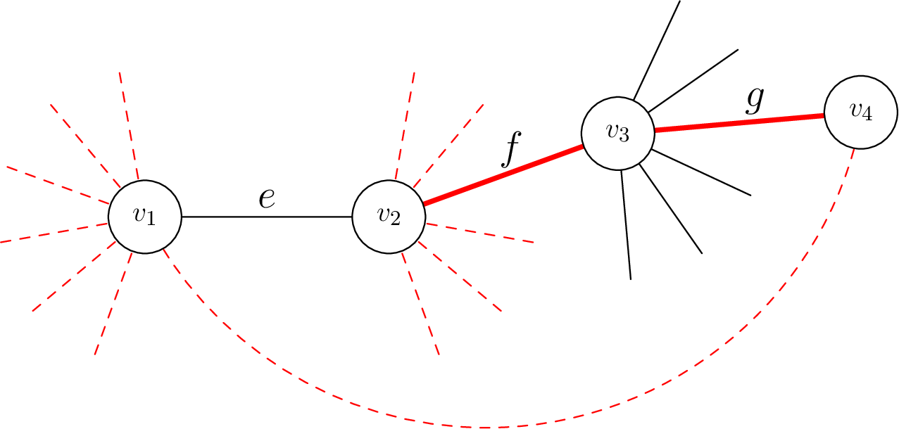
Figure 1: Our witness for $\mathds{1}[e\in\mu\wedge R_{1}(e)]$.

(a) Dashed edges are edges not realized before time $t_{e}$, while bold edges are realized before time $t_{e}$.

Fix any edge $g$ incident on $v_{3}$ and not incident on $e$, as in Figure 1(a). First, we note that conditioning on $Q(e)=\{f\}$ and specific arrival times (formalized below) does not decrease the probability of event $R_{0}(g)$, namely that zero edges incident on $g$ both arrive before $f$ and are realized.

Observation 3.4.

For any $0\leq c\leq b\leq a\leq 1$, we have

$$\Pr[R_{0}(g)\mid Q(e)=\{f\},t_{e}=a,t_{f}=b,t_{g}=c]\geq\Pr[R_{0}(g)\mid t_{g}=c]\geq\texttt{e}^{-(2-2x_{g})y}.$$

The above observation removes the conditioning on events for edges other than $g$; it is useful when lower bounding the conditional probability that $g$ is matched and arrives before $f$.

Lemma 3.5.

For any $0\leq b\leq a\leq 1$ we have

$$\Pr[g\in\mu,t_{g}\leq t_{f}\mid Q(e)=\{f\},t_{e}=a,t_{f}=b]\geq x_{g}\cdot\frac{1}{2}(1-2\alpha)\cdot(1-\texttt{e}^{-2b}).$$

Proof.

Edge $g$ is matched if it is realized and $R_{0}(g)$ occurs. On the other hand, conditioned on $Q(e)=\{f\},t_{e}=a,\,t_{f}=b,\,t_{g}=c$, the event that $g$ is realized is independent of $R_{0}(g)$, and has probability $x_{g}\cdot\texttt{e}^{-x_{g}c}\cdot(1-\alpha\cdot s_{g})$. Combined with 3.4, this yields the following.

$$\Pr[g\in\mu\mid Q(e)=\{f\},t_{e}=a,t_{f}=b,t_{g}=c] \geq x_{g}\cdot\texttt{e}^{-x_{g}c}\cdot(1-\alpha\cdot s_{g})\cdot\texttt{e}^{-(2-2x_{g})c}.$$

Therefore, by taking total probability over $g$’s arrival time $c\leq b$, we see that

$$\Pr[g\in\mu\wedge t_{g}\leq t_{f}\mid Q(e)=\{f\},t_{e}=a,t_{f}=b] \geq x_{g}\cdot(1-\alpha\cdot s_{g})\cdot\int_{0}^{b}\texttt{e}^{-(2-2x_{g})c}\texttt{e}^{-x_{g}c}\,dc$$

$$\geq x_{g}\cdot(1-2\alpha)\cdot\int_{0}^{b}\texttt{e}^{-2c}\,dc$$

$$=x_{g}\cdot\frac{1}{2}(1-2\alpha)\cdot(1-\texttt{e}^{-2b}),$$

where the second inequality relied on $s_{g}\leq 2$ and $x_{g}\geq 0$ implying $2-x_{g}\leq 2$. ∎

Next, fix an edge $f\in N_{e}$, and let $B_{f}$ denote the event that some edge $g\in N_{f}\setminus N_{e}$ with $t_{g}\leq t_{f}$ is matched (hence blocking edge $f$ from being matched). Note that the single edge $g\in N_{f}\cap N_{e}$ (if any) must have $x_{g}\leq m_{e}$, by definition of $m_{e}=\max\{x_{f}\mid f\in N_{e},\text{ there exists a triangle containing }e,f\}.$ As the events $\{g\in\mu\}$ are disjoint for distinct $g\in N_{f}\setminus N_{e}$, summing the individual bounds from Lemma 3.5 implies the following corollary.

Corollary 3.6.

For any $0\leq b\leq a\leq 1$ we have

$$\Pr[B_{f}\mid Q(e)=\{f\},t_{e}=a,t_{f}=b]\geq(d_{f}-m_{e}-1)^{+}\cdot\frac{1}{2}(1-2\alpha)\cdot(1-\texttt{e}^{-2b}).$$

For our analysis, we are concerned with the event that $R_{1}(e)$ occurs, and that the unique realized edge $f$ is blocked. We denote this event by $U_{e}:=\bigcup_{f\in N_{e}}[Q(e)=\{f\}\wedge B_{f}]$. The following lemma, whose proof is deferred to Appendix B, follows directly (after some calculation) from 3.6.

Lemma 3.7.

For any $a\in[0,1]$, we have that

$$Pr[U_{e}\mid t_{e}=a]\geq\frac{1}{2}(1-2\alpha)^{2}\sum_{f\in N_{e}}x_{f}(d_{f}-m_{e}-1)^{+}\cdot\texttt{e}^{-ad_{e}+ax_{f}}\cdot\left(\frac{1-\texttt{e}^{-x_{f}a}}{x_{f}}-\frac{1-\texttt{e}^{-a(x_{f}+2)}}{x_{f}+2}\right).$$

We are now ready to prove our main lemma.

Proof of Lemma 3.2.

Since $e$ is matched and $R_{1}(e)$ hold if $e$ is active and $U_{e}$ occurs (the latter two events being independent conditioned on the arrival time of $e$), we have

$$\Pr[e\in\mu\wedge R_{1}(e)] \geq x_{e}\cdot\int_{0}^{1}a_{2}(a,x_{e},s_{e})\cdot\Pr[U_{e}\mid t_{e}=a]\,da.$$

Let $z(x):=\int_{0}^{1}\texttt{e}^{-2a+ax_{f}}\left(\frac{1-\texttt{e}^{-xa}}{x}-\frac{1-\texttt{e}^{-a(x+2)}}{x+2}\right)\,da$. Substituting in our bound from Lemma 3.7 on $\Pr[U_{e}\mid t_{e}=a]$, and noting that $d_{e}+x_{e}\leq 2$, we find, after some rearranging, that

$$\Pr[e\in\mu\wedge R_{1}(e)]\geq x_{e}\cdot\frac{1}{2}(1-2\alpha)^{2}(1-\alpha\cdot s_{e})\sum_{f\in N_{e}}x_{f}(d_{f}-m_{e}-1)^{+}\cdot z(x_{f}).$$

We simplify this bound via the following numerical fact, whose proof is deferred to Appendix B.

Fact 3.8.

For any $x\in[0,1]$, we have that $x\cdot z(x)\geq 0.055x.$

Using this fact and substituting in $s_{f}=2-d_{f}-x_{f}$, we obtain the claimed bound.

$$\Pr[e\in\mu\wedge R_{1}(e)] \geq\left((1-\alpha\cdot s_{e})(1-2\alpha)^{2}\cdot\sum_{f\in N_{e}}x_{f}(1-m_{e}-x_{f}-s_{f})^{+}\cdot 0.0275\right)\cdot x_{e}.\qed$$

3.4 Reducing to a 5-variable problem

We improve upon the bound of $h(2)=\frac{1}{2}(1-\texttt{e}^{-2})$ by combining Lemma 3.1 and Lemma 3.2. For ease of reference, we restate these two lemmas here.

See 3.1 See 3.2

Proof idea of Theorem 1.2.

The following is an easy lower bound on the probability of $e$ being matched.

$$\Pr[e\in\mu]\geq\Pr[e\in\mu\wedge R_{0}(e)]+\Pr[e\in\mu\wedge R_{1}(e)]=(\star).$$

Here, $(\star)$ is the lower bound obtained by summing the lower bounds of lemmas 3.1 and 3.2. Before unpacking this (rather unwieldy) expression, we first simplify it as follows. First, we note that for $\alpha\geq 0.12$, the coefficient of $s_{f}$ in $(\star)$ is at least $x_{e}\cdot(1-\alpha\cdot s_{e})\cdot x_{f}(0.14\alpha-0.0275(1-2\alpha)^{2})\geq 0$. Recalling that $s_{f}\geq x_{f}$, we have that $(\star)$ is made no larger by replacing each occurrence of $s_{f}$ with $x_{f}$, resulting in a lower bound $(\star)\geq({\dagger})$.

To lower bound $({\dagger})$, we need a way to relate the $\sum_{f\in N_{e}}x_{f}^{2}$ to $m_{e}$. To do so, let

$$f^{*}:=\arg\max_{f\in N_{e}}\{x_{f}:\text{ there exists a triangle containing }e,f\}.$$

So, $x_{f^{*}}=m_{e}$, with the possibility that $f^{*}=\emptyset$ if $m_{e}=0$. Let $N_{e}^{*}$ denote $N_{e}\setminus\{f^{*}\}$, and define $d^{\text{big}}_{e}:=\sum_{f\in N_{e}^{*}:x_{f}\geq(1-m_{e})/2}x_{f}$ to be the contribution to $d_{e}$ due to edges with $x$-value at least $(1-m_{e})/2$. In $({\dagger})$, the coefficients of $x_{f}^{2}$ for $f\in N_{e}^{*}$ with $x_{f}<(1-m_{e})/2$ are given by $0.14\alpha-2\cdot 0.0275(1-2\alpha)^{2}$, which is positive for $\alpha\geq 0.171$. Using also that $d^{\text{big}}_{e}\cdot\frac{1-m_{e}}{2}\leq\sum_{f\in N_{e}:x_{f}\geq(1-m_{e})/2}x_{f}^{2}$ we have that $({\dagger})$ is lower bounded by

$$(1-\alpha\cdot s_{e})\left(h(2)+0.14\left(s_{e}+\alpha m_{e}^{2}+\alpha\cdot d^{\text{big}}_{e}\cdot\frac{1-m_{e}}{2}\right)+0.0275(1-2\alpha)^{2}\cdot(d_{e}-d^{\text{big}}_{e})\cdot(1-m_{e})\right)x_{e}.$$

We conclude that the algorithm’s balancedness for fixed $\alpha\in[0.171,0.5]$ is at least the solution to the following five-variable optimization problem.

$$\min \enspace(1-\alpha\cdot s_{e})\Big{(}h(2)+0.14\left(s_{e}+\alpha m_{e}^{2}+\alpha\cdot d^{\text{big}}_{e}\cdot\frac{1-m_{e}}{2}\right)+0.0275(1-2\alpha)^{2}\cdot(d_{e}-d^{\text{big}}_{e})\cdot(1-m_{e})\Big{)}$$

s.t. $$s_{e}+d_{e}=2-x_{e}$$

$$d_{e}\geq d^{\text{big}}_{e}$$

$$d_{e}\leq 2(1-x_{e})$$

$$m_{e}\leq 1$$

$$x_{e},s_{e},d_{e},d^{\text{big}}_{e},m_{e}\geq 0.$$

Numeric simulations with $\alpha=0.171$ yield a lower bound of $0.45$. Furthermore, in the bipartite case, we have only a four-variable optimization problem, as $m_{e}$ can be fixed at 0. In this case, numeric simulations yield a lower bound of $0.456$. ∎

4 Stochastic OCRS for Matching with Patience

In this section, we show that our approach can also be used to improve on the current state-of-the-art algorithm for the patience-constrained setting frequently studied in the stochastic probing literature. In this extension of our problem, each vertex $u$ has an integer patience constraint $\ell_{u}$, specifying that at most $\ell_{u}$ edges incident on $u$ can be probed. By Lemma 2.5, we restrict our attention in this section to the stochastic OCRS model as in 2.4. For the remainder of this section, we use the notation $x_{e}:=y_{e}\cdot p_{e}$ (recall that $\vec{x}$ is in the matching polytope by 2.4).

Our goal in this section is to prove the following theorem.

See 1.3

Let $B_{u}$ be the event that vertex $u$ is blocked, either by an edge incident on $u$ being matched or $u$ running out of patience. A useful lemma for us, proven by Brubach et al. [BGMS21, Lemma 2] for the generic Algorithm 3, is that the worst-case bound for $\Pr[\bar{B}_{u}]$ is achieved when for all edges $e$ incident on $u$, we have $p_{e}\in\{0,1\}$.

Lemma 4.1 ([BGMS21]).

For any vertex $u$, the value of $\Pr[\bar{B}_{u}]$ is made no larger by assuming that for all edges $e\ni u$, we have $p_{e}\in\{0,1\}$.

The intuition behind this lemma is that for any edge $e\ni u$ with $p_{e}\in(0,1)$, if we split it into two edges with probabilities 0 and 1, then the corresponding LP solution is still feasible and $\Pr[B_{u}]$ does not decrease. Let $E_{0}(u)$ and $E_{1}(u)$ denote the set of edges $e\ni u$ with $p_{e}=0$ and $p_{e}=1$, respectively.

4.1 Analysis for General Graphs

In the patience-constrained setting, we show that our new attenuation function $a_{2}(\cdot)$ can be used to improve on the state-of-the-art $0.382$-approximate algorithm of [BGMS21]. We briefly note that if we use the attenuation function $a_{1}(\cdot)$ from Section 2.1 instead of $a_{2}(\cdot)$ in Algorithm 3, we will get the same approximation ratio as in [BGMS21, Section 3] with a similar analysis. To analyze Algorithm 3 with patience constraints, we have the same high-level intuition as in Section 3: for each edge $e$ we will provide a lower bound for $\Pr[e\in\mu\wedge R_{0}(e)]$ and $\Pr[e\in\mu\wedge R_{1}(e)]$.

4.1.1 Lower bounding $\Pr[e\in\mu\wedge R_{0}(e)]$

First, we provide a lower bound for the event that no edges in $N_{e}$ arrived before $e$ and were realized, and $e$ was matched.

Lemma 4.2.

For each edge $e\in E$, we have the following.

$$\Pr[e\in\mu\wedge R_{0}(e)]\geq(1-\alpha\cdot s_{e})\left(0.382+0.117\left(s_{e}+\alpha\cdot\sum_{f\in N_{e}}x_{f}s_{f}\right)\right)\cdotp x_{e}.$$

Proof.

By Lemma 4.1, we can assume that all edges incident on $e$ have integer success probabilities. There are two cases for edge $e=(uv)$ to be blocked: (i) some edge $f\in E_{1}(u)\cup E_{1}(v)$ arrives before $e$ and is realized, or (ii) $u$ or $v$ loses patience before $e$ is considered because of the probing of edges in $E_{0}(u)\cup E_{0}(v)$. (Note that any edge $E_{1}(u)\cup E_{1}(v)$ that we probe is successful, while edges in $E_{0}(u)\cup E_{0}(v)$ cannot be realized.) Define $\ell_{u}(e):=\{f\ni u\mid f\in E_{0}(u),\,t_{f}<t_{e}\}$. Then, note that if $\ell_{u}(e)\leq l_{u}-1$, which is independent of the event that $e$ is blocked by (i), it is not possible that $e$ is blocked by $u$ having lost patience despite being free (a similar statement holds for $v$). Putting it together, we have

$$\Pr[R_{0}(e)\wedge\{u,v\}\textrm{ have patience}\mid t_{e}=y]$$

$$\geq \Pr[R_{0}(e)\mid t_{e}=y]\Pr[\ell_{u}(e)\leq\ell_{u}-1]\Pr[\ell_{v}(e)\leq\ell_{v}-1].$$

As in the proof of Lemma 3.1, we have that

$$\Pr[R_{0}(e)\mid t_{e}=y]\geq\texttt{e}^{-y(d_{e}-\alpha\cdot\sum_{f\in N_{e}}x_{f}s_{f})}.$$

Furthermore, by [BCN⁺18, Lemma 11], $\Pr[\ell_{u}(e)\leq\ell_{u}-1]$ is minimized when $\ell_{u}(e)\sim\text{ Pois}(y(\ell_{u}-1))$. Let $\phi_{\ell_{u}}(y):=\Pr[\ell_{u}(e)\leq\ell_{u}-1]$ when $\ell_{u}(e)\sim\text{ Pois}(y(\ell_{u}-1))$. Thus

$$\Pr[R_{0}(e)\wedge\{u,v\}\textrm{ has patience}\mid t_{e}=y]\geq\texttt{e}^{-y(d_{e}-\alpha\cdot\sum_{f\in N_{e}}x_{f}s_{f})}\cdot\phi_{\ell_{u}}(y)\cdot\phi_{\ell_{v}}(y).$$

We finish the proof by taking total expectation over the time $e$ arrives:

$$\Pr[e\in\mu\wedge R_{0}(e)] =x_{e}\cdot(1-\alpha\cdot s_{e})\cdot\int_{0}^{1}\Pr[R_{0}(e)\wedge\{u,v\}\textrm{ have patience}\mid t_{e}=y]\cdot\texttt{e}^{-x_{e}y}\,dy$$

$$\geq x_{e}\cdot(1-\alpha\cdot s_{e})\cdot\int_{0}^{1}\texttt{e}^{-y(d_{e}-\alpha\cdot\sum_{f\in N_{e}}x_{f}s_{f})-x_{e}y}\cdot\phi_{\ell_{u}}(y)\cdot\phi_{\ell_{v}}(y)\,dy.$$ (7)

Based on numerical simulations, we can show that the above is minimized when $\ell_{u}=2$ and $\ell_{v}=2$, yielding the following.

$$\Pr[e\in\mu\wedge R_{0}(e)] \geq x_{e}\cdot(1-\alpha\cdot s_{e})\cdot\int_{0}^{1}\texttt{e}^{-y(2-\alpha\cdot\sum_{f\in N_{e}}x_{f}s_{f})}\cdot(\texttt{e}^{-y}+y\texttt{e}^{-y})^{2}\cdot\,dy$$

$$=x_{e}\cdot(1-\alpha\cdot s_{e})\cdot\int_{0}^{1}\texttt{e}^{-y(4-s_{e}-\alpha\cdot\sum_{f\in N_{e}}x_{f}s_{f})}\cdot(1+y)^{2}\,dy.$$

$$\geq(1-\alpha\cdot s_{e})\left(0.382+0.117\left(s_{e}+\alpha\cdot\sum_{f\in N_{e}}x_{f}s_{f}\right)\right)\cdot x_{e},$$

where the last step is captured by Fact C.1, whose proof is deferred to Appendix C. ∎

Note that for $\alpha=0$, Algorithm 1 captures the [BGMS21] result. By choosing $\alpha>0$, we can guarantee that the bound in Lemma 4.2 is larger than 0.382 if $s_{e}$ or $\sum_{f\in N(e)}x_{f}s_{f}$ is large.

4.1.2 Lower bounding $\Pr[e\in\mu\wedge R_{1}(e)]$

In this section, we lower bound the probability that $e$ is matched despite a neighboring edge $f$ being realized and appearing before $e$, because $f$ is blocked.

Lemma 4.3.

For each edge $e\in E$, we have the following.

$$\Pr[e\in\mu\wedge R_{1}(e)]\geq\left((1-2\alpha)^{2}(1-\alpha\cdot s_{e})\cdot\sum_{f\in N_{e}}x_{f}(1-m_{e}-x_{f}-s_{f})^{+}\cdot 0.02\right)\cdot x_{e}.$$

Note that the difference between the analysis of this section and Section 3.3 is that when $g\in N_{f}$ which is incident on $v_{3}$ arrives before $f$, vertex $v_{4}$ must have remaining patience in order to argue that $f$ gets blocked by $g$. If $v_{4}$ has lost patience, $g$ will not block $f$, resulting in $e$ possibly not being free (even if conditioning on the fact that the only realized edge before $e$ is $f$). We prove a sequence of lemmas which help in the proof of Lemma 4.3.

By Lemma 4.1, we can assume that all edges that are incident on $v_{4}$ excluding $g$, have integer success probabilities since it does not decrease $\Pr[B_{v_{4}}]$. Let $B_{f}$ be the probability that edge $f$ is blocked, either by an edge $g$ incident on $v_{3}$ or because $v_{3}$ ran out of patience. Then we have the following lemma and corollary that help to provide a lower bound for this event.

Lemma 4.4.

For any $0\leq b\leq a\leq 1$ we have

$$\Pr[g\in\mu,t_{g}\leq t_{f}\mid Q(e)=\{f\},t_{e}=a,t_{f}=b,\ell_{v_{3}}(f)\leq\ell_{v_{3}}-1]\geq x_{g}\cdot\frac{(1-2\alpha)\cdot(4-(3b+4)\texttt{e}^{-3b})}{9}.$$

Corollary 4.5.

For any $0\leq b\leq a\leq 1$ we have

$$\Pr[B_{f}\mid Q(e)=\{f\},t_{e}=a,t_{f}=b] \geq(d_{f}-m_{e}-1)^{+}\cdot(1-2\alpha)\cdot\frac{1}{9}\cdot(1-(3b+4)\texttt{e}^{-3b}).$$

We defer the proofs of the above lemma and corollary to Appendix C. Let $U_{e}$ denote the event that there is a unique edge $f$ in $Q(e)$, and furthermore that $B_{f}$ occurs ($U_{e}:=\bigcup_{f\in N_{e}}[Q(e)=\{f\}\wedge B_{f}]$). The following lemma, whose proof is similar to the proof of Lemma 3.7, and is therefore deferred to Appendix C, lower bounds the probability of $U_{e}$ conditioned on the arrival time of edge $e$.

Lemma 4.6.

For any $a\in[0,1]$,

$$Pr[U_{e}\mid t_{e}=a]\geq\frac{1}{9}(1-2\alpha)^{2}\sum_{f\in N_{e}}x_{f}(d_{f}-m_{e}-1)^{+}\cdot\texttt{e}^{-ad_{e}+ax_{f}}\cdot h_{1}(a,x_{f}),$$

where $h_{1}(a,x_{f}):=\int_{0}^{a}\texttt{e}^{-bx_{f}}\cdot(4-(3b+4)\texttt{e}^{-3b})\,db$.

With this in place, we can complete the proof of Lemma 4.3.

Proof of Lemma 4.3.

Equipped with Lemma 4.6, we are ready to provide a lower bound for $\Pr[e\in\mu\wedge R_{1}(e)]$ by taking total expectation over the time $e$ arrives:

$$\Pr[e\in\mu\wedge R_{1}(e)] \geq x_{e}\cdot a_{2}(t_{e},x_{e},s_{e})$$

$$\cdot\int_{0}^{1}\Pr[U_{e}\mid t_{e}=a]\cdot\Pr[\ell_{v}(e)\leq\ell_{v}-1\mid t_{e}=a]\cdot\Pr[\ell_{u}(e)\leq\ell_{u}-1\mid t_{e}=a]\,da,$$

which is minimized when $\Pr[\ell_{u}(e)\leq\ell_{u}-1]$ minimized when $\ell_{u}(e)\sim\text{ Pois}(y(\ell_{u}-1))$ by [BCN⁺18, Lemma 11]. Assuming $\phi_{\ell_{u}}(y):=\Pr[\ell_{u}(e)\leq\ell_{u}-1]$ when $\ell_{u}(e)\sim\text{ Pois}(y(\ell_{u}-1))$, and $h_{1}(a,x_{f})=\int_{0}^{a}\texttt{e}^{-bx_{f}}\cdot(4-(3b+4)\texttt{e}^{-3b})\,db$, we have that

$$\Pr[e\in\mu\wedge R_{1}(e)] \geq\frac{1}{9}\cdot x_{e}\cdot(1-2\alpha)^{2}(1-\alpha\cdot s_{e})$$

$$\cdot\int_{0}^{1}\texttt{e}^{-ax_{e}}\sum_{f\in N_{e}}x_{f}(d_{f}-m_{e}-1)^{+}\cdot\texttt{e}^{-ad_{e}+ax_{f}}\cdot h_{1}(a,x_{f})\cdot\phi_{\ell_{u}}(a)\cdot\phi_{\ell_{v}}(a)\,da,$$ (8)

which is minimized when $\ell_{u}=2$ and $\ell_{v}=2$. Then

$$\Pr[e\in\mu\wedge R_{1}(e)]$$

$$\geq\frac{1}{9}\cdot x_{e}(1-2\alpha)^{2}(1-\alpha\cdot s_{e})\sum_{f\in N_{e}}x_{f}(d_{f}-m_{e}-1)^{+}\int_{0}^{1}\texttt{e}^{-ax_{e}-ad_{e}+ax_{f}}\cdot h_{1}(a,x_{f})(e^{-a}+ae^{-a})^{2}\,da$$

$$\geq\frac{1}{9}\cdot x_{e}(1-2\alpha)^{2}(1-\alpha\cdot s_{e})\sum_{f\in N_{e}}x_{f}(d_{f}-m_{e}-1)^{+}\int_{0}^{1}\texttt{e}^{-4a+ax_{f}}\cdot h_{1}(a,x_{f})\cdot(1+a)^{2}\,da$$

$$\geq\frac{1}{9}\cdot x_{e}(1-2\alpha)^{2}(1-\alpha\cdot s_{e})\sum_{f\in N_{e}}x_{f}(d_{f}-m_{e}-1)^{+}\cdot 0.181.$$

In the last inequality, we used Fact 4.7 to simplify the integral.

Fact 4.7.

Let $h_{1}(a,x_{f})=\int_{0}^{a}\texttt{e}^{-bx_{f}}\cdot(4-(3b+4)\texttt{e}^{-3b})\,db$. Then we have

$$\int_{0}^{1}\texttt{e}^{-4a+ax_{f}}\cdot h_{1}(a,x_{f})\cdot(1+a)^{2}\,da\geq 0.181.$$

Writing this in terms of $s_{f}=2-d_{f}-x_{f}$, we have

$$\Pr[e\in\mu\wedge R_{1}(e)] \geq\left((1-2\alpha)^{2}(1-\alpha\cdot s_{e})\cdot\sum_{f\in N_{e}}x_{f}(1-m_{e}-x_{f}-s_{f})^{+}\cdot 0.02\right)\cdot x_{e}.\qed$$

4.2 Analysis for Bipartite Graphs with Patience Constraints on One Side

In this section, we assume that the input graph is bipartite and we have patience constraints on only the vertices on one side (as motivated by applications in the gig economy).

We show that with a small modification to the analysis for general graphs with patience, we can achieve a larger bound in the bipartite setting. We use Algorithm 3 and assume that patience number for vertices of one side is $\infty$. Note that all lemmas for general graphs also hold here. In order to get a better bound, we slightly change the analysis of Lemma 4.2 and Lemma 4.3 by assuming that only one endpoint of edge $e$ has a patience constraint. All the steps are similar to the analysis for general graphs with patience constraints and the only difference is the last steps in Lemma 4.2 and Lemma 4.3. We defer the complete proofs of the following two lemmas to the appendix.

Lemma 4.8.

For each edge $e\in E$, we have the following.

$$\Pr[e\in\mu\wedge R_{0}(e)]\geq(1-\alpha\cdot s_{e})\left(0.405+0.131\left(s_{e}+\alpha\cdot\sum_{f\in N_{e}}x_{f}s_{f}\right)\right)\cdot x_{e}.$$

Lemma 4.9.

For each edge $e\in E$, we have the following.

$$\Pr[e\in\mu\wedge R_{1}(e)]\geq\left((1-2\alpha)^{2}(1-\alpha\cdot s_{e})\cdot\sum_{f\in N_{e}}x_{f}(1-x_{f}-s_{f})^{+}\cdot 0.023\right)\cdot x_{e}.$$

Proof of Theorem 1.3.

Combining Lemma 4.2 and Lemma 4.3, for each edge $e$, we have the following lower bound for $\Pr[e\in\mu]/x_{e}$:

$$(1-\alpha\cdot s_{e})\cdot\left(0.382+0.117(s_{e}+\alpha\cdot\sum_{f\in N_{e}}x_{f}s_{f})+(1-2\alpha)^{2}\cdot\sum_{f\in N_{e}}x_{f}(1-m_{e}-x_{f}-s_{f})^{+}\cdot 0.02\right),$$

for general graphs with patience on all vertices. Similar to Section 3.4, numeric simulations with $\alpha=0.16$ yield a lower bound of $0.395$.

When the input graph is a bipartite graph with patience constraint on one part, by combining Lemma 4.8 and Lemma 4.9, for each edge $e$, we have the following lower bond for $\Pr[e\in\mu]/x_{e}$

$$(1-\alpha\cdot s_{e})\cdot\left(0.405+0.131(s_{e}+\alpha\cdot\sum_{f\in N_{e}}x_{f}s_{f})+(1-2\alpha)^{2}\cdot\sum_{f\in N_{e}}x_{f}(1-x_{f}-s_{f})^{+}\cdot 0.023\right),$$

for bipartite graphs with patience on one side. Numeric simulations with $\alpha=0.162$ yield a lower bound of $0.426$. ∎

5 Discussion

Our work developed a new RO-OCRS for matching and a new stochastic RO-OCRS for matching with patience constraints, and through this gave an approximation algorithm for the sequential pricing problem, with applications in the gig economy. We did so by designing a new attenuation function that takes into account how much contention an edge has for its endpoints. Our work leaves multiple interesting avenues for future research.

A natural question is whether there is a more principled manner to pick $a(e)$ without changing the core of our analysis. We required multiple non-trivial lower bounds relying on an explicit form for $a(e)$ which seem hard to generalize to symbolic $a(e)$, but it is likely there is already room for improvement here. It would also be very interesting to extend our analysis by considering the probabilities of events $\Pr[e\in\mu\wedge R_{k}(e)]$ for $k\geq 2$.

Our algorithm, as well as all prior work on (RO-)OCRS for matching constraints, works with the degree-bounded relaxation for matchings, which is integral for bipartite graphs, but not for general ones. A natural question is whether better (RO-)OCRS can be achieved for points in the matching polytope, i.e., points which also satisfy Edmonds’ odd-set constraints [Edm65]. Can better bounds be achieved for this polytope, perhaps via a different algorithmic approach?

Finally, we note that in the sequential pricing problem, we have complete control over the ordering in which we consider the edges; while RO-OCRS is a natural algorithmic primitive with many distinct applications, for our application the constraint that we consider edges in a uniformly random is self-imposed. Can a better approximation be achieved by considering edges in an order that is not uniformly random?

Acknowledgements.

This research was funded in part by NSF CCF1812919. We thank anonymous reviewers for their useful comments.

Appendix A Omitted Proofs of Section 2

See 2.5

Proof.

Define $y_{e}:=\sum_{w}y_{ew}$ and $p_{e}:=\frac{\sum_{w}y_{ew}p_{ew}}{\sum_{w}y_{ew}}$; note that $(y_{e})$ and $(p_{e})$ form a valid input to a Stochastic OCRS algorithm by the constraints of LP-Pricing. Suppose that before running Algorithm 1, we sample for each edge $e=(ij)$ and price $w$ independent Bernoulli variables $A_{ew}\sim\text{Ber}(p_{ew})$ in advance, along with the weights $\{\pi_{e}\}$. (This clearly does not change the outcome of the algorithm.) Now, imagine that we run Algorithm 3 on the instance given by $\vec{y},\vec{p}$ in the following way: we probe $e$ with probability $a(e)$ if and only if there exists some $w$ such that $\pi_{e}=w$, and we assume $e$ is active if and only if $A_{e\pi_{e}}=1$. Note then when running Algorithm 3 in this way, we probe $e$ with probability $\left(\sum_{w}y_{ew}\right)\cdot a(e)=y_{e}\cdot a(e)$. Additionally, the probability $e$ is active conditioned on it being probed is precisely $\frac{\sum_{w}y_{ew}p_{ew}}{\sum_{w}y_{ew}}=p_{e}$.

So, by the $c$-balancedness of Algorithm 3, we know that $\Pr[e\in\mu]=c^{\prime}\cdot y_{e}\cdot p_{e}$, for some $c^{\prime}\geq c$. Recall that $e$ is matched if and only if it is active (i.e., $A_{e\pi_{e}}=1$), when processed it is free and has endpoints with patience, and an independent Bernoulli variable $\text{Ber}(a(e))$ comes up heads. Since these latter two events are independent of $e$’s active status, we have that $\Pr[e\in\mu\mid e\text{ active}]=c^{\prime}$. Indeed, since the joint event that $e$ is free and has endpoints with patience when processed, and $\text{Ber}(a(e))=1$ are both independent of $\pi_{e}$ and all the $A_{ew}$ variables, we have that for each $w$,

$$\Pr[e\in\mu\mid\pi_{e}=w\wedge A_{e\pi_{e}}=1]=\Pr[e\in\mu\mid A_{e\pi_{e}}=1]=c^{\prime}.$$

Consequently, the expected revenue satisfies the following:

$$\mathbb{E}\left[\sum_{j\in A}v_{j}-\sum_{e\in\mu}\pi_{e}\right] =\sum_{ij}\sum_{w}(v_{j}-w)\cdot c^{\prime}\cdot\Pr[\pi_{e}=w]\cdot\Pr[A_{e\pi_{e}}=1\mid\pi_{e}=w]$$

$$=\sum_{ij}\sum_{w}(v_{j}-w)\cdot c^{\prime}\cdot y_{ew}\cdot p_{ew}$$

$$=c^{\prime}\cdot OPT(\text{{LP-Pricing}})\geq c\cdot OPT(\text{{LP-Pricing}}).$$

Combining the above with Lemma 2.1, the lemma follows. ∎

Appendix B Omitted Proofs of Section 3

See 3.4

Proof.

Since arrival times and realization status are independent, the LHS above is precisely $\Pr[R_{0}(g)\mid Q(e)=\{f\},t_{e}=a,t_{f}=b,t_{g}=c]=\prod_{e^{\prime}\in N_{g}\setminus N_{e}}\Pr[e^{\prime}\text{ not realized and arrived by time }c]$. The first inequality follows since the second term is precisely the same product taken over all edges in $N_{g}$, and is therefore no greater. Finally, the last inequality follows from our choice of attenuation function $a_{2}(g)\leq a_{1}(g)$, and therefore by the same argument as in the proof of Lemma 2.7, the probability that zero realized edges $g^{\prime}\in N_{g}$ arrive before time $t_{g}$, is no smaller than under the attenuation function $a_{1}(\cdot)$, as calculated in Equation 6. ∎

See 3.6

Proof.

The events $E_{g}:=[g\in\mu,t_{g}\leq t_{f}]$ for $g\ni v_{3}$ are disjoint, since $v_{3}$ is matched at most once. Moreover, $B_{f}\supseteq\bigcup_{g\ni v_{3},g\not\in N_{e}}E_{g}$. Therefore,

$$\Pr[B_{f}\mid Q(e)=\{f\},t_{e}=a,t_{f}=b] \geq\sum_{g\ni v_{3},\,g\not\in N_{e}}\Pr[E_{g}\mid Q(e)=\{f\},t_{e}=a,t_{f}=b]$$

$$\geq\sum_{g\ni v_{3},\,g\not\in N_{e}}x_{g}\cdot\frac{1}{2}(1-2\alpha)\cdot(1-\texttt{e}^{-2b})$$

$$\geq(d_{f}-m_{e}-1)^{+}\cdot\frac{1}{2}(1-2\alpha)\cdot(1-\texttt{e}^{-2b}),$$

where the last inequality follows from the definition of $d_{f}=\sum_{g\in N_{f}}x_{g}$ together with the matching constraint $\sum_{g\ni v_{3},g\neq f}x_{g}\leq 1$ and the definition of $m_{e}$. ∎

See 3.7

Proof.

Fix an edge $f$. First, observe that the probability all edges $e^{\prime}\in N_{e}\setminus\{f\}$ are either not realized or arrive after $t_{e}=a$ is

$$\Pr[Q(e)\subseteq\{f\}\mid t_{e}=a] =\prod_{e^{\prime}\in N_{e}\setminus\{f\}}\left(1-\int_{0}^{a}x_{e^{\prime}}\cdot a_{2}(b,x_{e^{\prime}},s_{e^{\prime}})\,db\right)$$

$$\geq\prod_{e^{\prime}\in N_{e}\setminus\{f\}}\left(1-\int_{0}^{a}x_{e^{\prime}}\cdot\texttt{e}^{-bx_{e^{\prime}}}\,db\right)$$

$$=\texttt{e}^{-a\left(\sum_{e^{\prime}\in N_{e}\setminus\{f\}}x_{e^{\prime}}\right)}$$

$$\geq\texttt{e}^{-ad_{e}+ax_{f}}.$$

Also, the events $\{Q(e)=\{f\}\mid f\in N_{e}\}$ are disjoint, since $Q(e)=\{f\}$ implies that $f$ is the unique realized edge incident on $e$ arriving before $t_{e}$. Hence, using 3.6, we have

$$\Pr[U_{e}\mid t_{e}=a] \geq\sum_{f\in N_{e}}\int_{0}^{a}x_{f}\cdot a_{2}(b,x_{f},s_{f})\cdot\texttt{e}^{-ad_{e}+ax_{f}}\cdot\Pr[B_{f}\mid Q(e)=\{f\},t_{e}=a,t_{f}=b]\,db$$

$$\geq\sum_{f\in N_{e}}\int_{0}^{a}x_{f}\cdot a_{2}(b,x_{f},s_{f})\cdot\texttt{e}^{-ad_{e}+ax_{f}}\cdot(d_{f}-m_{e}-1)^{+}\cdot\frac{1}{2}(1-2\alpha)(1-\texttt{e}^{-2b})\,db$$

$$=\frac{1}{2}(1-2\alpha)(1-\alpha\cdot s_{f})\sum_{f\in N_{e}}x_{f}(d_{f}-m_{e}-1)^{+}\cdot\texttt{e}^{-ad_{e}+ax_{f}}\cdot\int_{0}^{a}\texttt{e}^{-bx_{f}}\cdot(1-\texttt{e}^{-2b})\,db$$

$$\geq\frac{1}{2}(1-2\alpha)^{2}\sum_{f\in N_{e}}x_{f}(d_{f}-m_{e}-1)^{+}\cdot\texttt{e}^{-ad_{e}+ax_{f}}\cdot\left(\frac{1-\texttt{e}^{-x_{f}a}}{x_{f}}-\frac{1-\texttt{e}^{-a(x_{f}+2)}}{x_{f}+2}\right).\qed$$

See 3.8

Proof.

If $x=0$ the bound clearly holds. Otherwise, let $x\in(0,1]$. We first directly compute that

$$\int_{0}^{1}\texttt{e}^{-2a+ax}\left(\frac{1-\texttt{e}^{-xa}}{x}-\frac{1-\texttt{e}^{-a(x+2)}}{x+2}\right)\,da =\frac{2\texttt{e}^{2}(x^{2}-4)-(x-2)x_{f}-\texttt{e}^{4}(x+2)x+8\texttt{e}^{x+2}}{4\texttt{e}^{4}x(x^{2}-4)}$$

$$=\left(\frac{2\texttt{e}^{2}(x^{2}-4)+8\texttt{e}^{x+2}}{4\texttt{e}^{4}x(x^{2}-4)}\right)-\frac{1}{4\texttt{e}^{4}(x+2)}-\frac{1}{4(x-2)}$$

Clearly $-\frac{1}{4(x-2)}\geq\frac{1}{8}$ and $-\frac{1}{4\texttt{e}^{4}(x+2)}\geq-\frac{1}{8\texttt{e}^{4}}$ for $x\in(0,1]$. Additionally, we observe that $\frac{2\texttt{e}^{2}(x^{2}-4)+8\texttt{e}^{x+2}}{4\texttt{e}^{4}x(x^{2}-4)}$ is a decreasing function in $x$ for $x\in(0,1]$. Hence

$$\frac{2\texttt{e}^{2}(x^{2}-4)+8\texttt{e}^{x+2}}{4\texttt{e}^{4}x(x^{2}-4)}\geq\lim_{x\rightarrow 0}\frac{2\texttt{e}^{2}(x^{2}-4)+8\texttt{e}^{x+2}}{4\texttt{e}^{4}x(x^{2}-4)}=-\frac{1}{2\texttt{e}^{2}}.$$

Hence, for $x\in(0,1]$ we have

$$\int_{0}^{1}\texttt{e}^{-2a+ax}\left(\frac{1-\texttt{e}^{-xa}}{x}-\frac{1-\texttt{e}^{-a(x+2)}}{x+2}\right)\,da\geq \frac{1}{8}-\frac{1}{8\texttt{e}^{4}}-\frac{1}{2\texttt{e}^{2}}\geq 0.055.\qed$$

Appendix C Omitted Proofs of Section 4

Fact C.1.

$\int_{0}^{1}\texttt{e}^{-y(4-s_{e}-\alpha\cdot\sum_{f\in N_{e}}x_{f}s_{f})}\cdot(1+y)^{2}\,dy\geq 0.382+0.117\left(s_{e}+\alpha\cdot\sum_{f\in N_{e}}x_{f}s_{f}\right)$.

Proof.

Let $K=s_{e}+\alpha\cdot\sum_{f\in N_{e}}x_{f}s_{f}$. Since $s_{e}+\alpha\cdot\sum_{f\in N_{e}}x_{f}s_{f}\geq 0$, we need to show that for $K\geq 0$,

$$\int_{0}^{1}\texttt{e}^{-y(4-K)}\cdot(1+y)^{2}\,dy\geq 0.382+0.117K.$$

Let $g(K)=\int_{0}^{1}\texttt{e}^{-y(4-K)}\cdot(1+y)^{2}\,dy$. First, note that $g$ is increasing in $K$; hence, the minimum occurs at $K=0$,

$$g(0)=\int_{0}^{1}\texttt{e}^{-y(4-0)}\cdot(1+y)^{2}\,dy\geq 0.382.$$

Moreover, by taking derivative of $g$, we have

$$g^{\prime}(K)=\frac{(K^{2}-12K+38)+e^{K-4}(4K^{3}-56K^{2}+266K-430)}{(K-4)^{4}},$$

which is an increasing function of $K$. Hence, $g^{\prime}$ minimized at $K=0$ on $[0,\infty)$. Therefore, we have $g^{\prime}(K)\geq g^{\prime}(0)\geq 0.117$, which completes the proof. ∎

See 4.4

Proof.

Similar to the proof of the Lemma 3.5, edge $g$ is matched if it is realized, $R_{0}(g)$ occurs, and $v_{4}$ has patience since we condition on $\ell_{v_{3}}(f)\leq\ell_{v_{3}}-1$. Since, the event that $g$ is active and $R_{0}(g)$ are independent, we have that

$$\Pr[g\in\mu\mid Q(e)=\{f\},t_{e}=a,t_{f}=b,t_{g}=c,\ell_{v_{3}}(f)\leq\ell_{v_{3}}-1]$$

$$\geq x_{g}\cdot a_{2}(c,x_{g},s_{g})\cdot\Pr[R_{0}(g)\wedge\ell_{v_{4}}(g)\leq\ell_{v_{4}}-1\mid Q(e)=\{f\},t_{e}=a,t_{f}=b,t_{g}=c,\ell_{v_{3}}(f)\leq\ell_{v_{3}}-1].$$

Since arrival times and activation status are independent, we have that

$$\Pr[g\in\mu\mid Q(e)=\{f\},t_{e}=a,t_{f}=b,t_{g}=c,\ell_{v_{3}}(f)\leq\ell_{v_{3}}-1]$$

$$\geq x_{g}\cdot a_{2}(c,x_{g},s_{g})\cdot\Pr[R_{0}(g)\wedge\ell_{v_{4}}(g)\leq\ell_{v_{4}}-1\mid t_{g}=c]$$

$$\geq x_{g}\cdot a_{2}(c,x_{g},s_{g})\cdot\Pr[R_{0}(g)\mid t_{g}=c]\cdot\Pr[\ell_{v_{4}}(g)\leq\ell_{v_{4}}-1\mid t_{g}=c]$$

$$\geq x_{g}\cdot\texttt{e}^{-x_{g}c}\cdot(1-\alpha\cdot s_{g})\cdot\texttt{e}^{-(2-2x_{g})c}\cdot\phi_{\ell_{v_{4}}}(c),$$

where $\phi_{\ell_{v_{4}}}(y):=\Pr[\ell_{v_{4}}(e)\leq\ell_{v_{4}}-1]$ when $\ell_{v_{4}}(e)\sim\text{ Pois}(y(\ell_{v_{4}}-1))$. By integrating over arrival time of $t_{g}\leq b$, we have that

$$\Pr[g\in\mu,t_{g}\leq t_{f} \mid Q(e)=\{f\},t_{e}=a,t_{f}=b,\ell_{v_{3}}(f)\leq\ell_{v_{3}}-1]$$

$$\geq x_{g}\cdot(1-\alpha\cdot s_{g})\cdot\int_{0}^{b}\texttt{e}^{-(2-2x_{g})c}\texttt{e}^{-x_{g}c}\cdot\phi_{\ell_{v_{4}}}(c)\,dc$$

$$\geq x_{g}\cdot(1-2\alpha)\cdot\int_{0}^{b}\texttt{e}^{-2c}\cdot\phi_{\ell_{v_{4}}}(c)\,dc.$$

Based on numerical simulations, we can show that the above is minimized when $\ell_{v_{4}}=2$, hence

$$\Pr[g\in\mu,t_{g}\leq t_{f} \mid Q(e)=\{f\},t_{e}=a,t_{f}=b,\ell_{v_{3}}(f)\leq\ell_{v_{3}}-1]$$

$$\geq x_{g}\cdot(1-2\alpha)\cdot\int_{0}^{b}\texttt{e}^{-3c}(1+c)\,dc$$

$$= x_{g}\cdot(1-2\alpha)\cdot\frac{1}{9}\cdot(4-(3b+4)\texttt{e}^{-3b}).\qed$$

See 4.5

Proof.

Note that the probability that $f$ is blocked condition on $\ell_{3}(f)\geq\ell_{3}$ is one. Moreover, conditional events $E_{g}:=\mathds{1}[g\in\mu,t_{g}\leq t_{f}]$ over all $g\ni v_{3}$ are disjoint. Thus, we have

$$\Pr[B_{f}\mid Q(e)=\{f\},t_{e}=a,t_{f}=b] \geq\Pr[B_{f}\mid Q(e)=\{f\},t_{e}=a,t_{f}=b,\ell_{v_{3}}(f)\leq\ell_{v_{3}}-1]$$

$$\geq\sum_{g\ni v_{3},\,g\not\notin N_{e}}\Pr[E_{g}\mid Q(e)=\{f\},t_{e}=a,t_{f}=b,\ell_{v_{3}}(f)\leq\ell_{v_{3}}-1]$$

$$\geq(d_{f}-m_{e}-1)^{+}\cdot(1-2\alpha)\cdot\frac{1}{9}\cdot(1-(3b+4)\texttt{e}^{-3b}),$$

where the last inequality is followed by Lemma 4.4. ∎

See 4.6

Proof.

Similar to the proof of Lemma 3.7, the probability that for each $e^{\prime}\in N_{e}\setminus\{f\}$ either is not realized or arrives after $t_{e}=a$ is at least $\texttt{e}^{-ad_{e}+ax_{f}}$. Moreover, since events $\{Q(e)=f\}_{f}$ are disjoint, then $\Pr[\exists f\textup{ such that }Q(e)=\{f\}\wedge B_{f}\mid t_{e}=a]$ is at least

$$\sum_{f\in N_{e}}\left(\int_{0}^{a}x_{f}\cdot a_{2}(t_{f},x_{f},s_{f})\cdot\texttt{e}^{-ad_{e}+ax_{f}}\cdot\Pr[B_{f}\mid Q(e)=\{f\},t_{e}=a,t_{f}=b]\,db\right),$$

which by 4.5 is at least,

$$\sum_{f\in N_{e}}\int_{0}^{a}x_{f}\cdot a_{2}(t_{f},x_{f},s_{f})\cdot\texttt{e}^{-ad_{e}+ax_{f}}\cdot(d_{f}-m_{e}-1)^{+}\cdot(1-2\alpha)\cdot\frac{1}{9}\cdot(4-(3b+4)\texttt{e}^{-3b})\,db$$

$$=\frac{1}{9}\cdot(1-2\alpha)(1-\alpha\cdot s_{f})\sum_{f\in N_{e}}x_{f}(d_{f}-m_{e}-1)^{+}\cdot\texttt{e}^{-ad_{e}+ax_{f}}\cdot\left(\int_{0}^{a}\texttt{e}^{-bx_{f}}\cdot(4-(3b+4)\texttt{e}^{-3b})\,db\right)$$

$$\geq\frac{1}{9}\cdot(1-2\alpha)^{2}\sum_{f\in N_{e}}x_{f}(d_{f}-m_{e}-1)^{+}\cdot\texttt{e}^{-ad_{e}+ax_{f}}\cdot h_{1}(a,x_{f}).\qed$$

Fact C.2.

$\int_{0}^{1}\texttt{e}^{-y(3-s_{e}-\alpha\cdot\sum_{f\in N_{e}}x_{f}s_{f})}\cdot(1+y)\,dy\geq 0.405+0.131(s_{e}+\alpha\cdot\sum_{f\in N_{e}}x_{f}s_{f}).$

Proof.

All steps of the proof are the same as in the proof of Fact C.1. Let $K=s_{e}+\alpha\cdot\sum_{f\in N_{e}}x_{f}s_{f}$ and $g(K)=\int_{0}^{1}\texttt{e}^{-y(3-K)}\cdot(1+y)\,dy$. We note that $g(\cdot)$ is an increasing function of $K$, so the minimum occurs at $K=0$, where

$$g(0)=\int_{0}^{1}\texttt{e}^{-y(3-0)}\cdot(1+y)\,dy\geq 0.405.$$

Also, we have that

$$g^{\prime}(K)=\frac{(K-5)+e^{K-3}(2K^{2}-15K+29)}{(K-e)^{3}}.$$

Note that $g^{\prime}$ is an increasing function of $K$ that is minimized at $K=0$ on $[0,\infty)$. Therefore, we have $g^{\prime}(K)\geq g^{\prime}(0)\geq 0.131$, which completes the proof. ∎

See 4.7

Proof sketch.

This fact is verified computationally by direct calculation of the integral. ∎

See 4.8

Proof.

With the exact same analysis as in Lemma 4.2, we have Section 4.1.1. Now without loss of generality, let $v$ be the vertex such that $\ell_{v}=\infty$. Hence, we have $\phi_{\ell_{v}}(y)=1$. Therefore,

$$\Pr[e\in\mu\wedge R_{0}(e)] \geq x_{e}\int_{0}^{1}\texttt{e}^{-y(d_{e}-\alpha\cdot\sum_{f\in N_{e}}x_{f}s_{f})}\cdot\phi_{\ell_{u}}(y)\cdot\texttt{e}^{-x_{e}y}\cdot(1-\alpha\cdot s_{e})\,dy.$$

Based on numerical simulations, we can show that the above is minimized when $t_{u}=2$, yielding the following

$$\Pr[e\in\mu\wedge R_{0}(e)] \geq x_{e}\cdot(1-\alpha\cdot s_{e})\cdot\int_{0}^{1}\texttt{e}^{-y(d_{e}-\alpha\cdot\sum_{f\in N_{e}}x_{f}s_{f})}\cdot(\texttt{e}^{-y}+y\texttt{e}^{-y})\cdot\texttt{e}^{-x_{e}y}\,dy$$

$$=x_{e}\cdot(1-\alpha\cdot s_{e})\cdot\int_{0}^{1}\texttt{e}^{-y(3-s_{e}-\alpha\cdot\sum_{f\in N_{e}}x_{f}s_{f})}\cdot(1+y)\,dy,$$

which can be simplified by Fact C.2. Therefore, we have that

$$\Pr[e\in\mu\wedge R_{0}(e)] \geq(1-\alpha\cdot s_{e})\left(0.405+0.131\left(s_{e}+\alpha\cdot\sum_{f\in N_{e}}x_{f}s_{f}\right)\right)\cdot x_{e}.\qed$$

Fact C.3.

Let $h_{1}(a,x_{f})=\int_{0}^{a}\texttt{e}^{-bx_{f}}\cdot(4-(3b+4)\texttt{e}^{-3b})\,db$. Then we have

$$\int_{0}^{1}\texttt{e}^{-3a+ax_{f}}\cdot h_{1}(a,x_{f})\cdot(1+a)\,da\geq 0.209.$$

Proof sketch.

This fact is verified computationally by direct calculation of the integral. ∎

See 4.9

Proof.

With exact same analysis of Lemma 4.3, we have Section 4.1.2. Without a loss of generality, let $v$ be the vertex such that $\ell_{v}=\infty$. Thus $\phi_{\ell_{v}}(a)=1$, yielding the following

$$\Pr[e\in\mu\wedge R_{1}(e)] \geq x_{e}\cdot\frac{1}{9}\cdot(1-2\alpha)^{2}(1-\alpha\cdot s_{e})$$

$$\cdot\int_{0}^{1}\texttt{e}^{-ax_{e}}\sum_{f\in N_{e}}x_{f}(d_{f}-1)^{+}\cdot\texttt{e}^{-ad_{e}+ax_{f}}\cdot h_{1}(a,x_{f})\cdot\phi_{\ell_{u}}(a)\,da,$$

where $h_{1}(a,x_{f})=\int_{0}^{a}\texttt{e}^{-bx_{f}}\cdot(4-(3b+4)\texttt{e}^{-3b})\,db$. Based on numerical simulations, we can show that the above is minimized when $t_{u}=2$, yielding the following

$$\Pr[e\in\mu\wedge R_{1}(e)]$$

$$\geq x_{e}\cdot\frac{1}{9}(1-2\alpha)^{2}(1-\alpha\cdot s_{e})\sum_{f\in N_{e}}x_{f}(d_{f}-1)^{+}\int_{0}^{1}\texttt{e}^{-ax_{e}}\texttt{e}^{-ad_{e}+ax_{f}}\cdot h_{1}(a,x_{f})\cdot(e^{-a}+ae^{-a})\,da$$

$$\geq x_{e}\cdot\frac{1}{9}(1-2\alpha)^{2}(1-\alpha\cdot s_{e})\sum_{f\in N_{e}}x_{f}(d_{f}-1)^{+}\int_{0}^{1}\texttt{e}^{-3a+ax_{f}}\cdot h_{1}(a,x_{f})\cdot(1+a)\,da$$

$$\geq x_{e}\cdot\frac{1}{9}(1-2\alpha)^{2}(1-\alpha\cdot s_{e})\sum_{f\in N_{e}}x_{f}(d_{f}-1)^{+}\cdot 0.209.$$

In the last inequality, we used Fact C.3 to simplify the integral. Writing this in terms of $s_{f}=2-d_{f}-x_{f}$, we have

$$\Pr[e\in\mu\wedge R_{1}(e)] \geq\left((1-2\alpha)^{2}(1-\alpha\cdot s_{e})\cdot\sum_{f\in N_{e}}x_{f}(1-x_{f}-s_{f})^{+}\cdot 0.023\right)\cdot x_{e}.\qed$$

Appendix D Ruling Out Natural Algorithms

D.1 Greedy According to Decreasing Weights

If there is only one weight for each edge, then by sorting the edges based on their weights and querying in that order, we can achieve a half approximation. However, this greedy algorithm achieves no constant approximation if we have multiple weights for one edge. Consider a single edge with two different weights, one and two, with probabilities one and $\varepsilon$, respectively. The greedy algorithm will gets a matching with expected weight of $2\varepsilon$, however, the optimal algorithm solution has expected size of one.

D.2 Greedy According to Decreasing Expected Weights

One can modify this greedy algorithm in the previous subsection to query edges based on decreasing order of $w\cdot p_{ew}$. But this modified version achieves no constant approximation; Consider a star with edges $e_{0},e_{1},\ldots,e_{k}$ with a single weight per edge such that $w_{e_{0}}=1+\varepsilon$ and $w_{e_{i}}=N^{i}$ for $1\leq i\leq k$. Also, we have that $p_{e_{i}}=1/N^{i}$. The modified greedy algorithm will get a matching with expected size of $1+\varepsilon$ (picks $e_{0}$) but an algorithm that asks edges in the order of $(e_{k},e_{k-1},\ldots,e_{1},e_{0})$ will get a matching with expected size of roughly equal to $k$. Since we can make $k$ as large as we want, then the modified greedy is not a constant approximation.

D.3 Trivial Attenuation is $1/3$-balanced

In this section we consider the simplest instantiation of Algorithm 1: the one with no attenuation, i.e., with $a(e)=1$ for all $e\in E$. Bruggmann and Zenklusen [BZ20] show that this algorithm is $\frac{1}{3}$-balanced. The following simpler analysis recreates the same bound.

Lemma D.1.

Denote by $\Pr[e\textup{ free}]$ the probability that $e=(i,j)$ is free when inspected. Then,

$$\Pr[e\textup{ free}]\geq\frac{1}{3}.$$

Proof.

For this instantiation of Algorithm 1, each edge $e$ is matched iff it is free (at time $t_{e})$. And indeed, we have the following.

$$\Pr[e\textup{ free}] \geq\Pr[R_{0}(e)]=\int_{0}^{1}\prod_{f\in N_{e}}(1-z\cdot x_{f})\,\,dz\geq\int_{0}^{1}(1-z\cdot(1-x_{e}))^{2}\,\,dz\geq\int_{0}^{1}(1-z)^{2}\,\,dz=\frac{1}{3},$$

where the second inequality relied on Fact D.2 below, combined with the matching constraint $\sum_{f\ni v}x_{f}\leq 1-x_{e}$ for both vertices $v\in e$. The third inequality follows from non-negativity of $x_{e}.$ ∎

The following fact is easily proven by induction.

Fact D.2.

Let $R_{1},R_{2},\dots,R_{n}\geq 0$. Then $\prod_{i=1}^{n}(1-R_{i})\geq 1-\sum_{i=1}^{n}R_{i}$.

The constant $1/3$ is tight for the algorithm without attenuation (see [BZ20, Figure 6]).

Appendix E Reduction to Single Weight without Patience with a $\nicefrac{{1}}{{2}}$-Factor Loss

In this section, we show that after solving LP-Pricing (with $\ell_{v}=\infty$ for all $v$), we can incur a multiplicative loss of no worse than $1/2$ and reduce the problem to the case where for each edge $e$, there is only one weight $w$ where $y_{ew}>0$.

We first prove that there exists an optimal solution to our LP where each edge’s $y$-values are supported on at most two weights.

Lemma E.1.

There exists an optimal solution $\vec{y}^{\prime}$ to our LP where for any edge $e$, there are at most two different weights $w_{1}$ and $w_{2}$ such that $y^{\prime}_{ew_{1}}>0$ and $y^{\prime}_{ew_{2}}>0$.

Proof.

Let $\vec{y}^{*}$ denote an optimal solution to our LP, and recall our notation $x_{e}=\sum_{w}y^{*}_{ew}\cdot p_{ew}$. For a fixed edge $e$, consider the following LP for variables $\{y_{ew}\}_{w}$:

$$\max \sum_{w}y_{ew}\cdot p_{ew}\cdot(v_{j}-w)$$

s.t. $$\sum_{w}y_{ew}\leq 1$$

$$\sum_{w}y_{ew}\cdot p_{ew}\leq x_{e}$$

$$y_{ew}\geq 0.$$

Any linear program in standard form with maximization objective function has an optimal solution at an extreme point. Since we have only two non-trivial constraints in the above LP, any extreme point has at most two non-zero values. Let $\vec{y}^{\prime}$ denote this solution; note furthermore that replacing $y^{*}_{ew}$ with $y^{\prime}_{ew}$ for all $w$ in our original LP results in a solution that is still feasible and has no loss in objective. ∎

Now for each edge $e$, let $W(e)$ denote the weight $w$ that maximizes $y_{ew}\cdot p_{ew}\cdot(v_{j}-w)$. Since there exists an optimal solution $\vec{y}^{\prime}$ with only two non-zero weights for each edge, we have that

$$y_{eW(e)}\cdot p_{eW(e)}\cdot W(e)\geq\frac{1}{2}\cdot\sum_{w}y_{ew}\cdot p_{ew}\cdot(v_{j}-w)$$

Therefore, any $\alpha$-approximate algorithm for LP solutions with a single weight on each edge, results in an $\alpha/2$-approximation algorithm for our original problem.

Appendix F Random Vertex Arrival

In the random vertex arrival setting, vertices of one side of the bipartite graph are present at the beginning. Vertices of the other side arrive one by one in random order with their incident edges. In this setting, after a vertex arrives, an online algorithm can probe incident edges to build a matching. Note that the algorithm is only allowed to probe feasible edges that do not violate matching constraints.

Similar to Section 2.1, we let $\{x_{e}\}_{e\in E}$ denote the realization probabilities in the random vertex arrival. Note that in this setting, we cannot sort edges based on a random time $t_{e}\sim\text{Unif}[0,1]$ for each edge because edges that are incident on a specific online vertex arrive together. Therefore, we use a random time $t_{u}\sim\text{Unif}[0,1]$ for each online vertex $u$ and we sort edges based on the tuple $(t_{u},t_{e})$ where $u$ is the online endpoint of edge $e$.

1for each edge $e$, sample a random time $t_{e},t_{u}\sim\text{Unif}[0,1]$ for every edge $e$ and every online vertex $u$

2for each edge $e$, in increasing order of $(t_{u},t_{e})$ where $u$ is its online endpoint do

3       if $e$ is active and is free then

4             with probability $s(x_{e},t_{e},t_{u})$, match $e$.

Algorithm 4

We use the same attenuation function $e^{-x_{e}t_{e}}$ as Section 2.1. Note that this attenuation function is not dependent on $t_{u}$.

Lemma F.1.

When running Algorithm 4 with $s(x_{e},t_{e},t_{u})=\texttt{e}^{-t_{e}x_{e}}$, the probability we sell along edge $e$ is at least $(1-1/\texttt{e})^{2}\geq 0.399\cdot x_{e}$.

Proof.

Let $N_{u}$ be the set of edges incident on vertex $u$. Let $e=(u,v)$ where $u$ is online endpoint and $v$ is the offline endpoint. There are two types of edges that can block $e$: 1) $f\in N_{u}\setminus\{e\}$ such that $t_{f}<t_{f}$. 2) $g=(w,v)\in N_{v}\setminus\{e\}$ such that $t_{w}<t_{u}$. Hence, if we condition on edge $e=(u,v)$ with $t_{e}=y_{1}$ and online endpoint arrival time $t_{u}=y_{2}$, we have the following inequality

$$\Pr[e\textrm{ free}\mid t_{e}=y_{1},t_{u}=y_{2}]\geq\prod_{f\in N_{u}}\left(1-\int_{0}^{y_{1}}x_{f}\cdot\texttt{e}^{-x_{f}z}\,dz\right)\prod_{g\in N_{v}}\left(1-y_{2}\cdot\int_{0}^{1}x_{g}\cdot\texttt{e}^{-x_{g}z}\,dz\right).$$ (9)

The reason is that if an $f=(u,v^{\prime})$ blocks $e$, it must arrive before $t_{e}$, edge $f$ must survive the attenuation step, and $f$ must be successful after the proposal. Moreover, for an edge $g=(u^{\prime},v)$ to block $e$, online endpoint $u^{\prime}$ must arrive before $t_{u}$ (note that $t_{g}$ does not play a role on whether $g$ arrives before $e$), it must survive the attenuation step, and $g$ must be succseful after the proposal. Equation 9 follows by the fact that all these events are independent. Then we have that

$$\Pr[e\textrm{ free}\mid t_{e}=y_{1},t_{u}=y_{2}] \geq\prod_{f\in N_{u}}\left(1-\int_{0}^{y_{1}}x_{f}\cdot\texttt{e}^{-x_{f}z}\,dz\right)\prod_{g\in N_{v}}\left(1-y_{2}\cdot\int_{0}^{1}x_{g}\cdot\texttt{e}^{-x_{g}z}\,dz\right)$$

$$=\prod_{f\in N_{u}}\texttt{e}^{-x_{f}y_{1}}\prod_{g\in N_{v}}\left(1-y_{2}\cdot(1-\texttt{e}^{-x_{g}})\right)$$

By Fact 3.3, we have $\left(1-y_{2}\cdot(1-\texttt{e}^{-x_{g}})\right)\geq\texttt{e}^{-x_{g}y_{2}}$. Therefore we have the following.

$$\Pr[e\textrm{ free}\mid t_{e}=y_{1},t_{u}=y_{2}] \geq\prod_{f\in N_{u}}\texttt{e}^{-x_{f}y_{1}}\prod_{g\in N_{v}}\left(1-y_{2}\cdot(1-\texttt{e}^{-x_{g}})\right)$$

$$\geq\prod_{f\in N_{u}}\texttt{e}^{-x_{f}y_{1}}\prod_{g\in N_{v}}\texttt{e}^{-x_{f}y_{1}}$$

$$=\texttt{e}^{-y_{1}(1-x_{e})}\cdot\texttt{e}^{-y_{2}(1-x_{e})}=\texttt{e}^{-(1-x_{e})(y_{1}+y_{2})}.$$

Hence, we have that

$$\Pr[e\textrm{ successful}] =\Pr[e\text{ free at }(t_{u},t_{e})\text{ and }\text{Ber}(s(x_{e},t_{e},t_{u}))=1]\cdot x_{e}$$

$$\geq\left(\int_{0}^{1}\int_{0}^{1}\texttt{e}^{-(1-x_{e})(y_{1}+y_{2})}\cdot\texttt{e}^{-y_{1}x_{e}}dy_{1}dy_{2}\right)\cdot x_{e}$$

$$\geq\left(\int_{0}^{1}\int_{0}^{1}\texttt{e}^{-(y_{1}+y_{2})}dy_{1}dy_{2}\right)\cdot x_{e}$$

$$\geq\left(1-\frac{1}{\texttt{e}}\right)^{2}\cdot x_{e}\geq 0.399\cdot x_{e}.\qed$$

References

- [ABG+20] Marek Adamczyk, Brian Brubach, Fabrizio Grandoni, Karthik A Sankararaman, Aravind Srinivasan, and Pan Xu. Improved approximation algorithms for stochastic-matching problems. arXiv preprint arXiv:2010.08142, 2020.
- [Ada11] Marek Adamczyk. Improved analysis of the greedy algorithm for stochastic matching. Information Processing Letters (IPL), 111(15):731–737, 2011.
- [Ada15] Marek Adamczyk. Non-negative submodular stochastic probing via stochastic contention resolution schemes. arXiv preprint arXiv:1508.07771, 2015.
- [ADSY12] Shipra Agrawal, Yichuan Ding, Amin Saberi, and Yinyu Ye. Price of correlations in stochastic optimization. Operations Research, 60(1):150–162, 2012.
- [AGM15] Marek Adamczyk, Fabrizio Grandoni, and Joydeep Mukherjee. Improved approximation algorithms for stochastic matching. In Proceedings of the 23rd Annual European Symposium on Algorithms (ESA), pages 1–12. 2015.
- [ASW16] Marek Adamczyk, Maxim Sviridenko, and Justin Ward. Submodular stochastic probing on matroids. Mathematics of Operations Research, 41(3):1022–1038, 2016.
- [AW18] Marek Adamczyk and Michał Włodarczyk. Random order contention resolution schemes. In Proceedings of the 59th Symposium on Foundations of Computer Science (FOCS), pages 790–801, 2018.
- [BCN+18] Alok Baveja, Amit Chavan, Andrei Nikiforov, Aravind Srinivasan, and Pan Xu. Improved bounds in stochastic matching and optimization. Algorithmica, 80(11):3225–3252, 2018.
- [BGL+12] Nikhil Bansal, Anupam Gupta, Jian Li, Julián Mestre, Viswanath Nagarajan, and Atri Rudra. When lp is the cure for your matching woes: Improved bounds for stochastic matchings. Algorithmica, 63(4):733–762, 2012.
- [BGMS21] Brian Brubach, Nathaniel Grammel, Will Ma, and Aravind Srinivasan. Improved guarantees for offline stochastic matching via new ordered contention resolution schemes. In Proceedings of the 35th Annual Conference on Neural Information Processing Systems (NeurIPS), 2021.
- [BSSX20] Brian Brubach, Karthik A Sankararaman, Aravind Srinivasan, and Pan Xu. Attenuate locally, win globally: Attenuation-based frameworks for online stochastic matching with timeouts. Algorithmica, 82(1):64–87, 2020.
- [BZ20] Simon Bruggmann and Rico Zenklusen. An optimal monotone contention resolution scheme for bipartite matchings via a polyhedral viewpoint. Mathematical Programming, pages 1–51, 2020.
- [CGM13] Marek Cygan, Fabrizio Grandoni, and Monaldo Mastrolilli. How to sell hyperedges: The hypermatching assignment problem. In Proceedings of the 25th Annual ACM-SIAM Symposium on Discrete Algorithms (SODA), pages 342–351, 2013.
- [CHMS10] Shuchi Chawla, Jason D Hartline, David L Malec, and Balasubramanian Sivan. Multi-parameter mechanism design and sequential posted pricing. In Proceedings of the 42nd Annual ACM Symposium on Theory of Computing (STOC), pages 311–320, 2010.
- [CIK+09] Ning Chen, Nicole Immorlica, Anna R Karlin, Mohammad Mahdian, and Atri Rudra. Approximating matches made in heaven. In Proceedings of the 36th International Colloquium on Automata, Languages and Programming (ICALP), pages 266–278, 2009.
- [CVZ14] Chandra Chekuri, Jan Vondrák, and Rico Zenklusen. Submodular function maximization via the multilinear relaxation and contention resolution schemes. SIAM Journal on Computing (SICOMP), 43(6):1831–1879, 2014.
- [Edm65] Jack Edmonds. Maximum matching and a polyhedron with {0,1}-vertices. Journal of research of the National Bureau of Standards B, 69(125-130):55–56, 1965.
- [EFGT20] Tomer Ezra, Michal Feldman, Nick Gravin, and Zhihao Gavin Tang. Online stochastic max-weight matching: prophet inequality for vertex and edge arrival models. In Proceedings of the 21st ACM Conference on Economics and Computation (EC), pages 769–787, 2020.
- [EHKS18] Soheil Ehsani, MohammadTaghi Hajiaghayi, Thomas Kesselheim, and Sahil Singla. Prophet secretary for combinatorial auctions and matroids. In Proceedings of the twenty-ninth annual acm-siam symposium on discrete algorithms, pages 700–714. SIAM, 2018.
- [FSZ16] Moran Feldman, Ola Svensson, and Rico Zenklusen. Online contention resolution schemes. In Proceedings of the 27th Annual ACM-SIAM Symposium on Discrete Algorithms (SODA), pages 1014–1033, 2016.
- [FTW+21] Hu Fu, Zhihao Gavin Tang, Hongxun Wu, Jinzhao Wu, and Qianfan Zhang. Random order vertex arrival contention resolution schemes for matching, with applications. In Proceedings of the 48th International Colloquium on Automata, Languages and Programming (ICALP), 2021.
- [GKS19] Buddhima Gamlath, Sagar Kale, and Ola Svensson. Beating greedy for stochastic bipartite matching. In Proceedings of the Thirtieth Annual ACM-SIAM Symposium on Discrete Algorithms, pages 2841–2854. SIAM, 2019.
- [GL18] Guru Guruganesh and Euiwoong Lee. Understanding the correlation gap for matchings. In Proceedings of the 37thFoundations of Software Technology and Theoretical Computer Science (FSTTCS), 2018.
- [GN13] Anupam Gupta and Viswanath Nagarajan. A stochastic probing problem with applications. In International Conference on Integer Programming and Combinatorial Optimization, pages 205–216. Springer, 2013.
- [GNS16] Anupam Gupta, Viswanath Nagarajan, and Sahil Singla. Algorithms and adaptivity gaps for stochastic probing. In Proceedings of the twenty-seventh annual ACM-SIAM symposium on Discrete algorithms, pages 1731–1747. SIAM, 2016.
- [GNS17] Anupam Gupta, Viswanath Nagarajan, and Sahil Singla. Adaptivity gaps for stochastic probing: Submodular and xos functions. In Proceedings of the Twenty-Eighth Annual ACM-SIAM Symposium on Discrete Algorithms, pages 1688–1702. SIAM, 2017.
- [GTW19] Nick Gravin, Zhihao Gavin Tang, and Kangning Wang. Online stochastic matching with edge arrivals. arXiv preprint arXiv:1911.04686, 2019.
- [GW19] Nikolai Gravin and Hongao Wang. Prophet inequality for bipartite matching: Merits of being simple and non adaptive. In Proceedings of the 20th ACM Conference on Economics and Computation (EC), pages 93–109, 2019.
- [KS81] Richard M Karp and Michael Sipser. Maximum matching in sparse random graphs. In Proceedings of the 22nd Symposium on Foundations of Computer Science (FOCS), pages 364–375, 1981.
- [KW19] Robert Kleinberg and S Matthew Weinberg. Matroid prophet inequalities and applications to multi-dimensional mechanism design. Games and Economic Behavior, 113:97–115, 2019.
- [LS18] Euiwoong Lee and Sahil Singla. Optimal online contention resolution schemes via ex-ante prophet inequalities. In Proceedings of the 26th Annual European Symposium on Algorithms (ESA), pages 57:1–57:14, 2018.
- [Luc17] Brendan Lucier. An economic view of prophet inequalities. ACM SIGecom Exchanges, 16(1):24–47, 2017.
- [XLH20] Tao Xiao, Zhengyang Liu, and Wenhan Huang. On the complexity of sequential posted pricing. In Proceedings of the 19th International Conference on Autonomous Agents and Multi-Agent Systems (AAMAS), pages 1521–1529, 2020.
- [Yan11] Qiqi Yan. Mechanism design via correlation gap. In Proceedings of the 22nd Annual ACM-SIAM Symposium on Discrete Algorithms (SODA), pages 710–719, 2011.