Annealed importance sampling for Ising models with mixed boundary conditions

Abstract.

This note introduces a method for sampling Ising models with mixed boundary conditions. As an application of annealed importance sampling and the Swendsen-Wang algorithm, the method adopts a sequence of intermediate distributions that keeps the temperature fixed but turns on the boundary condition gradually. The numerical results show that the variance of the sample weights is relatively small.

1. Introduction

This note is concerned with the Monte Carlo sampling of Ising models with mixed boundary conditions. Consider a graph $G=(V,E)$ with the vertex set $V$ and the edge set $E$. Assume that $V=I\cup B$, where $I$ is the subset of interior vertices and $B$ the subset of boundary vertices. Throughout the note, we use $i,j$ to denote the vertices in $I$ and $b$ for the vertices in $B$. In addition, $ij\in E$ denotes an edge between two interior vertices $i$ and $j$, while $ib\in E$ denotes an edge between an interior vertex $i$ and a boundary vertex $b$. The boundary condition is specified by $f=(f_{b})_{b\in B}$ with $f_{b}=\pm 1$. The Ising model with the boundary condition $f$ is the probability distribution $p_{\mathrm{V}}(\cdot)$ over the configurations $s=(s_{i})_{i\in I}$ of the interior vertex set $I$:

(1) $$p_{\mathrm{V}}(s)\sim\exp\left(\beta\sum_{ij\in E}s_{i}s_{j}+\beta\sum_{ib\in E}s_{i}f_{b}\right).$$

A key feature of these Ising models is that, for certain mixed boundary conditions, below the critical temperature the Gibbs distribution exhibits on the macroscopic scale different profiles.

Figure 1 showcases two such examples. On the left, the square Ising lattice has the $+1$ condition on the vertical sides but the $-1$ condition on the horizontal sides. The two dominant profiles are a $-1$ cluster linking two horizontal sides and a $+1$ cluster linking two vertical sides. On the right, the Ising lattice supported on a disk has the $+1$ condition on two disjoint arcs and the $-1$ condition on the other two. The two dominant profiles are shown in Figure 1(b). Notice that in each case, the two dominant profiles have comparable probability. Hence it is important for any sampling algorithm to visit both profiles frequently.

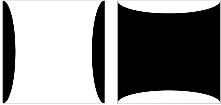
(a)	(b)

Figure 1. Ising models with mixed boundary conditions. (a) a square model and (b) a model support on a disk. In each case, a mixed boundary condition is specified and the model exhibits two dominant profiles on the macroscopic scale.

One of the most well-known methods for sampling Ising models is the Swendsen-Wang algorithm [swendsen1987nonuniversal], which will be briefly reviewed in Section 2. For Ising models free boundary condition for example, the Swendsen-Wang algorithm exhibits rapid mixing for all temperatures. However, for the mixed boundary conditions shown in Figure 1, the Swendsen-Wang algorithm experiences slow convergence under the critical temperatures, i.e., $T<T_{c}$ or equivalently $\beta>\beta_{c}$ in terms of the inverse temperature. The reason is that, for such a boundary condition, the energy barrier between the two dominant profiles is much higher than the energies of these profiles. In other words, the Swendsen-Wang algorithm needs to break a macroscopic number of edges between aligned adjacent spins in order to transition from one dominant profile to the other. However, breaking so many edges simultaneously is an event with exponentially small probability when the mixed boundary condition is specified.

Annealed importance sampling is a method by Radford Neal [neal2001annealed], designed for sampling distributions with multiple modes. The main idea is to (1) introduce an easily-to-sample simple distribution, (2) design a sequence of temperature dependent intermediate distributions, and (3) generate sample paths that connects the simple initial distribution and the hard target distribution. Annealed importance sampling has been widely applied in Bayesian statistics and data assimilation for sampling and estimating partition functions.

In this note, we address this problem by combining the Swendsen-Wang algorithm with annealed importance sampling. The main novelty of our approach is that, instead of adjusting the temperature, we freeze the temperature and adjust the mixed boundary condition.

Related works. In [alexander2001spectral, alexander2001spectralB], Alexander and Yoshida studied the spectral gap of the 2D Ising models with mixed boundary conditions. In [ying2022double], the double flip move is introduced for models with mixed boundary conditions that enjoy exact or approximate symmetry. When combined with the Swendsen-Wang algorithm, it can accelerate the mixing of these Ising model under the critical temperature significantly. However, it only applies to problem with exact or approximate symmetries, but not more general settings.

Recently in [gheissari2018effect], Gheissari and Lubetzky studied the effect of the boundary condition for the 2D Potts models at the critical temperature. In [chatterjee2020speeding], Chatterjee and Diaconis showed that most of the deterministic jumps can accelerate the Markov chain mixing when the equilibrium distribution is uniform.

Contents. The rest of the note is organized as follows. Sections 2 and 3 review the Swendsen-Wang algorithm and annealed importance sampling, respectively. Section 4 describes the algorithm and provides some numerical examples. Section 5 discusses some future directions.

2. Swendsen-Wang algorithm

In this section, we briefly review the Swendsen-Wang algorithm. First, notice that

$$p_{\mathrm{V}}(s)\sim\exp\left(\beta\sum_{ij\in E}s_{i}s_{j}+\beta\sum_{ib\in E}f_{b}s_{i}\right)=\exp\left(\beta\sum_{ij\in E}s_{i}s_{j}+\beta\sum_{i\in I}\left(\sum_{ib\in E}f_{b}\right)s_{i}\right).$$

Therefore, if we interpret $h_{i}=\sum_{ib\in E}f_{b}$ as an external field, one can view the mixed boundary condition problem as a special case of the model with external field $h=(h_{i})_{i\in I}$

(2) $$p_{\mathrm{V}}(s)\sim\exp\left(\beta\sum_{ij\in E}s_{i}s_{j}+\beta\sum_{i\in I}h_{i}s_{i}\right).$$

This viewpoint simplifies the presentation of the algorithm and the Swendsen-Wang algorithm is summarized below under this setting.

The Swendsen-Wang algorithm is a Markov Chain Monte Carlo method for sampling $p_{\mathrm{V}}(s)$. In each iteration, it generates a new configuration based on the current configuration $s$ with two substeps:

1. Generate an edge configuration $w=(w_{ij})_{ij\in E}$. If the spin values $s_{i}$ and $s_{j}$ are different, set $w_{ij}=0$. If $s_{i}$ and $s_{j}$ are the same, $w_{ij}$ is sampled from the Bernoulli distribution $\mathrm{Ber}(1-e^{-2\beta})$, i.e., equal to 1 with probability $1-e^{-2\beta}$ and 0 with probability $e^{-2\beta}$.

2. Regards all edges $ij\in E$ with $w_{ij}=1$ as linked. Compute the connected components. For each connected component $\gamma$, define $h_{\gamma}=\sum_{i\in\gamma}h_{i}$. Set the spins $(t_{i})_{i\in\gamma}$ of the new configuration $t$ to $1$ with probability $e^{\beta h_{\gamma}}/(e^{\beta h_{\gamma}}+e^{-\beta h_{\gamma}})$ and to $0$ with probability $e^{-\beta h_{\gamma}}/(e^{\beta h_{\gamma}}+e^{-\beta h_{\gamma}})$.

Associated with (2), two other probability distributions are important for analyzing the Swendsen-Wang algorithm [edwards1988generalization]. The first one is the joint vertex-edge distribution

(3) $$p_{\mathrm{VE}}(s,w)\sim\prod_{ij\in E}\left((1-e^{-2\beta})\delta_{s_{i}=s_{j}}\delta_{w_{ij}=1}+e^{-2\beta}\delta_{w_{ij}=0}\right)\cdot e^{\beta\sum_{i\in I}h_{i}s_{i}}.$$

The second one is the edge distribution

(4) $$p_{\mathrm{E}}(w)\sim\prod_{w_{ij}=1}(1-e^{-2\beta})\prod_{w_{ij}=0}e^{-2\beta}\cdot\prod_{\gamma\in\mathcal{C}_{w}}(e^{-\beta h_{\gamma}}+e^{\beta h_{\gamma}}),$$

where $\mathcal{C}_{w}$ is the set of the connected components induced by $w$.

Summing $p_{\mathrm{VE}}(s,w)$ over $s$ or $w$ gives the following two identities

(5) $$\sum_{s}p_{\mathrm{VE}}(s,w)=p_{\mathrm{E}}(w),\quad\sum_{w}p_{\mathrm{VE}}(s,w)=p_{\mathrm{V}}(s).$$

(see for example [edwards1988generalization]). A direct consequence of (5) is that the Swendsen-Wang algorithm can be viewed as a data augmentation method [liu2001monte]: the first substep samples the edge configuration $w$ conditioned on the spin configuration $s$, while the second substep samples a new spin configuration conditioned on the edge configuration $w$.

This equalities in (5) also imply that Swendsen-Wang algorithm satisfies the detailed balance. To see this, let us fix two spin configurations $s$ and $t$ and consider the the transition between them. Since such a transition in the Swendsen-Wang move happens via an edge configuration $w$, it is sufficient to show

$$p_{\mathrm{V}}(s)P_{w}(s,t)=p_{\mathrm{V}}(t)P_{w}(t,s)$$

for any compatible edge configuration $w$, where $P_{w}(s,t)$ is the transition probability from $s$ to $t$ via $w$. Since the transition probabilities from $w$ to the spin configurations $s$ and $t$ are proportional to $e^{\beta\sum_{i}h_{i}s_{i}}$ and $e^{\beta\sum_{i}h_{i}t_{i}}$ respectively, it reduces to showing

(6) $$p_{\mathrm{V}}(s)P(s,w)e^{\beta\sum_{i}h_{i}t_{i}}=p_{\mathrm{V}}(t)P(t,w)e^{\beta\sum_{i}h_{i}s_{i}},$$

where $P(s,w)$ is the probability of obtaining the edge configuration $w$ from $s$. Using (2), this is equivalent to

(7) $$e^{\beta\sum_{ij\in E}s_{i}s_{j}+\beta\sum_{i\in I}h_{i}s_{i}}P(s,w)e^{\beta\sum_{i\in I}h_{i}t_{i}}=e^{\beta\sum_{ij\in E}t_{i}t_{j}+\beta\sum_{i\in I}h_{i}t_{i}}P(t,w)e^{\beta\sum_{i\in I}h_{i}s_{i}}.$$

The next observation is that

(8) $$e^{\beta\sum_{ij\in E}s_{i}s_{j}}P(s,w)=e^{\beta\sum_{ij\in E}t_{i}t_{j}}P(t,w),$$

i.e., independent of the spin configuration, as explained below. First, if an edge $ij\in E$ has configuration $w_{ij}=1$, then $s_{i}=s_{j}$. Second, if $ij\in E$ has configuration $w_{ij}=0$, then $s_{i}$ and $s_{j}$ can either be the same or different. In the former case, the contribution to $e^{\beta\sum_{ij\in E}s_{i}s_{j}}P(s,w)$ from $ij$ is $e^{2\beta}\cdot e^{-2\beta}=1$ up to a uniform normalization constant. In the latter case, the contribution is also $1\cdot 1=1$ up to the same uniform constant. After canceling the two terms of (8) in (7), proving (6) is equivalent to $e^{\beta\sum_{i\in I}h_{i}s_{i}}\cdot e^{\beta\sum_{i\in I}h_{i}t_{i}}=e^{\beta\sum_{i\in I}h_{i}t_{i}}\cdot e^{\beta\sum_{i\in I}h_{i}s_{i}}$, which is trivial.

The Swendsen-Wang algorithm unfortunately does not encourage transitions between the dominant profiles shown for example in Figure 1. With these mixed boundary condition, such a transition requires breaking a macroscopic number of edges between aligned adjacent spins, which has an exponentially small probability.

3. Annealed importance sampling

Given a target distribution $p(s)$ that is hard to sample directly, annealed importance sampling (AIS), proposed by Neal in [neal2001annealed], introduces a sequence of distributions

$$p_{0}(\cdot),\ldots,p_{L}(\cdot)\equiv p(\cdot),$$

where $p_{0}(\cdot)$ is easy to sample and each $p_{l}(\cdot)$ is associated with a detailed balance Markov Chain $T_{l}(s,t)$, i.e.,

(9) $$p_{l}(s)T_{l}(s,t)=p_{l}(t)T_{l}(t,s).$$

The detailed balance condition can be relaxed, though it simplifies the description. Given this sequence of intermediate distributions, AIS proceeds as follows.

1. Sample a configuration $s_{1/2}$ from $p_{0}(\cdot)$.

2. For $l=1,\ldots,L-1$, take one step (or a few steps) of $T_{i}(\cdot,\cdot)$ (associated with the distributions $p_{l}(\cdot)$) from $s_{l-1/2}$. Let $s_{l+1/2}$ be the resulting configuration.

3. Set $s:=s_{L-1/2}$.

4. Set the weight

   $$w:=\frac{p_{1}(s_{1/2})}{p_{0}(s_{1/2})}\cdot\cdots\cdot\frac{p_{L}(s_{L-1/2})}{p_{L-1}(s_{L-1/2})}.$$

The claim is that the configuration $s$ with weight $w$ samples the target distribution $p_{L}(\cdot)$. To see this, consider the path $(s_{1/2},\ldots,s_{L-1/2})$. This path is generated with probability

$$p_{0}(s_{1/2})T_{1}(s_{1/2},s_{3/2})\ldots T_{L-1}(s_{L-3/2},s_{L-1/2}).$$

Multiplying this with $w$ and using the detailed balance (9) of $T_{l}$ gives

$$p_{0}(s_{1/2})T_{1}(s_{1/2},s_{3/2})\ldots T_{L-1}(s_{L-3/2},s_{L-1/2})\cdot\frac{p_{1}(s_{1/2})}{p_{0}(s_{1/2})}\cdot\cdots\cdot\frac{p_{L}(s_{L-1/2})}{p_{L-1}(s_{L-1/2})}$$

$$= p_{L}(s_{L-1/2})T_{L-1}(s_{L-1/2},s_{L-3/2})\ldots T_{1}(s_{3/2},s_{1/2}),$$

which is the probability of going backward, i.e., starting from a sample $s_{L-1/2}$ of $p_{L}(\cdot)=p(\cdot)$. Taking the margin of the last slot $s_{L-1/2}$ proves that $s:=s_{L-1/2}$ with weight $w$ samples with distribution $p_{L}(\cdot)=p(\cdot)$.

4. Algorithm and results

Our proposal is to combine AIS with the Swendsen-Wang algorithm for sampling Ising models with mixed boundary conditions. The key ingredients are:

• Set the initial $p_{0}(\cdot)$ to be

  $$p_{0}(s)\sim\exp\left(\beta\sum_{ij\in E}s_{i}s_{j}\right).$$

  This initial distribution has no external field and hence can be sampled efficiently with the Swendsen-Wang algorithm.

• Choose a monotone sequence of $(\theta_{l})_{0\leq l\leq L}$ with $\theta_{0}=0$ and $\theta_{L}=1$ and set at level $l$

  $$p_{l}(s)\sim\exp\left(\beta\sum_{ij\in E}s_{i}s_{j}+\beta\sum_{i\in I}(\theta_{l}h_{i})s_{i}\right),$$

  the distribution with external field $\theta_{h}h$. The Markov transition matrix $T_{l}(\cdot,\cdot)$ is implemented with the Swendsen-Wang algorithm associated with $p_{l}(\cdot)$. As proven in Section 2, $T_{l}(\cdot,\cdot)$ satisfies the detailed balance,

Below we demonstrate the performance of the proposed method with several examples. In each example, $K=500$ samples $(s^{(k)},w^{(k)})_{1\leq k\leq K}$ are generated. For each sample $s^{(k)}$, the initial choice $s^{(k)}_{1/2}$ is obtained by running $100$ iterations of the Swendsen-Wang algorithm at $p_{0}(\cdot)$. In our implementation, the monotone sequence $(\theta_{l})_{0\leq l\leq L}$ is chosen to be an equally spaced sequence with $L=400$. Although the equally-spaced sequence is not necessarily the ideal choice in terms of variance minimization, it seems to work reasonably well for the examples studied here.

In order to monitor the variance of the algorithm, we record the weight history at each level $l$:

$$w^{(k)}_{l}=\frac{p_{1}(s^{(k)}_{1/2})}{p_{0}(s^{(k)}_{1/2})}\cdot\cdots\cdot\frac{p_{l}(s^{(k)}_{l-1/2})}{p_{l-1}(s^{(k)}_{l-1/2})}$$

for $l=1,\ldots,L$. These weights are then normalized at each level $l$

$$\tilde{w}^{(k)}_{l}=\frac{1}{K}\sum_{k=1}^{K}w^{(k)}_{l}.$$

Following [neal2001annealed], we report the variance of the logarithm of the normalized weights $\text{Var}[\{\log\tilde{w}^{(k)}_{l}\}]$ as a function of level $l=1,\ldots,L$. The sample efficiency, a quantity between $0$ and $1$, is measured as $(1+\text{Var}[\{\tilde{w}^{(k)}_{L}\}])^{-1}$ at level $L$.

Example 1.

The Ising model is a square lattice, as shown in Figure 2(a). The mixed boundary condition is the $+1$ at the two vertical sides and $-1$ at the two horizontal sides. The experiments are performed for the problem size $n_{1}=n_{2}=40$ at the inverse temperature $\beta=0.5$. Figure 3(b) plots the variance of the logarithm of the normalized weights, $\text{Var}[\{\log\tilde{w}^{(k)}_{l}\}]$, as a function of the level $l$. The sample efficiency $(1+\text{Var}[\{\tilde{w}^{(k)}_{L}\}])^{-1}$ is $0.26$, which translates to $L\cdot(1+\text{Var}[\{\tilde{w}^{(k)}_{L}\}])^{-1}\approx 1530$ Swendsen-Wang iterations per effective sample.

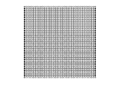
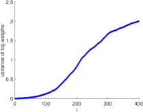
(a)	(b)

Figure 2. (a) The lattice along with the external field. (b) The variance of the logarithm of the normalized weights as a function of level $l$.

Example 2.

The Ising lattice is again a square as shown in Figure 3(a). The mixed boundary condition is $+1$ in the first and third quadrants but $-1$ in the second and fourth quadrants. The experiments are performed for the problem size $n_{1}=n_{2}=40$ at the inverse temperature $\beta=0.5$. Figure 3(b) plots $\text{Var}[\{\log\tilde{w}^{(k)}_{l}\}]$ as a function of the level $l$, which remain quite small. The sample efficiency $(1+\text{Var}[\{\tilde{w}^{(k)}_{L}\}])^{-1}$ is $0.09$, which translates to about $L\cdot(1+\text{Var}[\{\tilde{w}^{(k)}_{L}\}])^{-1}\approx 4470$ Swendsen-Wang iterations per effective sample.

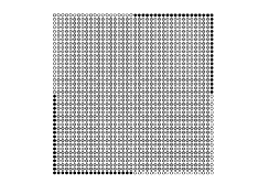
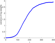
(a)	(b)

Figure 3. (a) The lattice along with the external field. (b) The variance of the logarithm of the normalized weights as a function of level $l$.

Example 3.

The Ising model is a random quasi-uniform triangular lattice supported on the unit disk, as shown in Figure 4(a). The lattice does not have rotation and reflection symmetry due to the random triangulation. The mixed boundary condition is $+1$ in the first and third quadrants but $-1$ in the second and fourth quadrants. The experiments are performed with a finer triangulation with mesh size $h=0.05$ at the inverse temperature $\beta=0.3$. Figure 4(b) plots $\text{Var}[\{\log\tilde{w}^{(k)}_{l}\}]$ as a function of the level $l$, which remain quite small. The sample efficiency $(1+\text{Var}[\{\tilde{w}^{(k)}_{L}\}])^{-1}$ is $0.67$, which translates to about $L\cdot(1+\text{Var}[\{\tilde{w}^{(k)}_{L}\}])^{-1}\approx 600$ Swendsen-Wang iterations per effective sample.

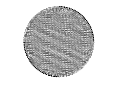
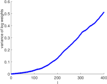
(a)	(b)

Figure 4. (a) The lattice along with the external field. (b) The variance of the logarithm of the normalized weights as a function of level $l$.

Example 4.

The Ising model is again a random quasi-uniform triangular lattice supported on the unit disk, as shown in Figure 5(a). The mixed boundary condition is $+1$ on the two arcs with angle in $[0,\pi/3]$ and $[\pi,5\pi/3]$ but $-1$ on the remaining two arcs. The experiments are performed with a finer triangulation with mesh size $h=0.05$ at the inverse temperature $\beta=0.3$. Figure 5(b) plots $\text{Var}[\{\log\tilde{w}^{(k)}_{l}\}]$ as a function of the level $l$, which remain quite small. The sample efficiency $(1+\text{Var}[\{\tilde{w}^{(k)}_{L}\}])^{-1}$ is $0.55$, which translates to about $L\cdot(1+\text{Var}[\{\tilde{w}^{(k)}_{L}\}])^{-1}\approx 730$ Swendsen-Wang iterations per effective sample.

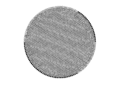
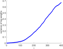
(a)	(b)

Figure 5. (a) The lattice along with the external field. (b) The variance of the logarithm of the normalized weights as a function of level $l$.

5. Discussions

This note introduces a method for sampling Ising models with mixed boundary conditions. As an application of annealed importance sampling with the Swendsen-Wang algorithm, the method adopts a sequence of intermediate distributions that fixes the temperature but turns on the boundary condition gradually. The numerical results show that the variance of the sample weights remain to be relatively small.

There are many unanswered questions. First, the sequence of $(\theta_{l})_{0\leq l\leq L}$ that controls the intermediate distributions is empirically specified to be equally-spaced. Two immediate questions are (1) what the optimal $(\theta_{l})_{0\leq l\leq L}$ sequence is and (2) whether there is an efficient algorithm for computing it.

Second, historically annealed importance sampling is introduced following the work of tempered transition [neal1996sampling]. We have implemented the current idea within the framework of tempered distribution. However, the preliminary results show that it is less effective compared to annealed importance sampling. A more thorough study is needed in this direction.

Finally, annealed importance sampling (AIS) is a rather general framework. For a specific application, the key to efficiency is the choice of the distribution $p_{0}(\cdot)$: it should be easy-to-sample, while at the same time sufficiently close to the target distribution $p(\cdot)$. However, since the target distribution is hard-to-sample, these two objectives often compete with each other. There are many other hard-to-sample models in statistical mechanics. A potential direction of research is to apply AIS with appropriate initial $p_{0}(\cdot)$ to these models.