A proposed network of Gamma-ray Burst detectors
on the Global Navigation Satellite System Galileo G2

The accurate localization of gamma-ray bursts remains a crucial task. While historically, improved localization have led to the discovery of afterglow emission and the realization of their cosmological distribution via redshift measurements, a more recent requirement comes with the potential of studying the kilonovae of neutron star mergers. Gravitational wave detectors are expected to provide locations to not better than 10 square degrees over the next decade. With their increasing horizon for merger detections also the intensity of the gamma-ray and kilonova emission drops, making their identification in large error boxes a challenge. Thus, a localization via the gamma-ray emission seems to be the best chance to mitigate this problem. Here we propose to equip some of the second generation Galileo satellites with dedicated GRB detectors. This saves costs for launches and satellites for a dedicated GRB network, the large orbital radius is beneficial for triangulation, and perfect positional and timing accuracy come for free. We present simulations of the triangulation accuracy, demonstrating that short GRBs as faint as GRB 170817A can be localized to 1 degree radius (1$\sigma$).

1 Introduction

The coincident detection of gravitational waves (GW) from a binary neutron star merger with aLIGO/Virgo and short-lived gamma-ray (GR) emission with Fermi-GBM (called GW 170817) in August 2017 is a milestone for the establishment of multi-messenger astronomy (Abbott et al., 2017), i.e. the measurement of electromagnetic radiation, gravitational waves and/or particles or neutrinos from the same astrophysical source. Merging neutron stars (NS) represent the standard scenario (Eichler et al., 1989) for short-duration ($<2$ s) gamma-ray bursts (sGRBs) which are produced in a collimated, relativistically expanding jet with an opening angle of a few degrees and a bulk Lorentz factor $\Gamma$ of 300–1000. While the aLIGO detection is consistent with predictions, the measured faint gamma-ray emission from GW 170817A is about 1000x less luminous than known short-duration GRBs. Hence, the presence of this sGRB in the local Universe is either a very rare event, or points to a dramatic mis-understanding of the emission properties of sGRBs outside their narrow jets. By now we know that the jet in this GRB had an opening angle of $<$5^∘, but we observed it from $\sim$20–30^∘ offaxis (Mooley et al., 2018). In all previous models, no emission was predicted to occur outside the opening angle.

Thus, also the previous estimates of the volume density of NS-NS mergers was wrong, and needs to be corrected (Burgess et al., 2020). This has important implications on our understanding of the chemical evolution of our Galaxy and the Universe, as NS-NS mergers are believed to be the main source of heavy elements (Kasen et al., 2017), so-called r-process elements (like gold and platinum). This material is expelled both during the tidal disruption of the NSs and through winds during the subsequent disk accretion onto the compact core. Further progress in our understanding of NS-NS mergers will depend on measurements in the electromagnetic regime, and these in turn will only be possible if the localizations of these events can be reduced to of order a few square degrees on the sky. While there exist several large-field-of-view optical sky surveys, covering up to several thousands square degrees, the challenge is to find the kilonova among the many other transient sources. Future NS-NS mergers will likely all(!) be at larger distance than GW 170817, and thus their kilonova much fainter. Already for the only 3x more distant four NS-NS merger events from 2019–2020, none detected in gamma-rays, the optical emission would peak at 23rd mag (if at identical luminosity as GW 170817). Except for one particularly poor localisation, the error regions of the other three events encompass 2300–14700 square degrees each (Wikipedia, 2020). At the expected optical brightness, there will be about 3–60 transient alerts per square degree down to 21 mag (Masci et al., 2019), or estimated 5x more at 23rd mag, against which the kilonova will have to be identified. Thus, a pre-requisite to identify the kilonova is the fast and precise localization of the GW/GR event.

Expectations for the fourth observing run O4 are 10${}^{+52}_{-10}$ BNS mergers, with a median 33${}^{+5}_{-5}$ square degrees localization. Likely not before 2026 (Abbott et al., 2020), the GW detector network of LIGO, Virgo and KAGRA is looking forward to include LIGO-India, which promises a reduction of the GW error regions to of order $<$10 square degrees. Further reduction of the localization error is foreseen with the Einstein Telescope in Europe, or the Cosmic Explorer in the USA, both not earlier than the mid 2030s.

Thus, accurate localization of the GW events should be sought elsewhere. Gamma-rays provide an interesting alternative, at least for those NS-NS mergers for which the jet would be broadly pointed towards us. With $\gamma$-ray emission at large off-axis angles as in GRB 170817A, up to 30% of mergers will be simultaneously detectable in $\gamma$-rays Howell et al. (2019); Burgess et al. (2020). Obviously, accurate measurements of many GRBs will be beneficial for other science questions beyond kilonova physics, such as (1) the structure of jets in GRBs (e.g., Janka et al., 2006) and the origin of the off-axis emission which is distinctly different to on-axis emission (Begue et al., 2017), or (2) the potential emission of high-energy neutrinos as measured by IceCube (Aartsen et al., 2013), promising a potential ’triple’-messenger, i.e. electromagnetic radiation, gravitational waves, and particles: Kimura et al. (2017) estimated that GRB 170817A could have been detectable by IceCube if the jet had been viewed on-axis instead of the $\sim$30^∘ off-axis.

Here, we propose adding a GRB detector on some of the next two dozen 2nd generation Galileo satellites (G2) in order to improve the localization capability for short GRBs to the 1-degree level, reducing the error region by a factor of 100–1000.

2 Prospects of accurate GRB localisation

2.1 Challenges of short GRBs

Short-duration GRBs (sGRB) have three properties which make their localisation in large numbers more difficult than that of long-duration GRBs:
(1) Their short duration, of order 0.01–2 s, implies that their observable fluence is of order 5–50x smaller than in long-duration GRBs.
(2) Their peak fluxes during their maximum spike is typically a factor 10 smaller than long-duration GRBs, making the discrepancy of (1) even larger.
(3) sGRBs are also harder, with their spectral peak at higher energies. This implies that the flux at soft gamma-rays (20–100 keV) is smaller than that in long-duration GRBs even if the energy-integrated flux is equal.

These factors together imply detection and localisation disadvantages in various detector types: (i) in coded-mask imagers like Swift/BAT or INTEGRAL/IBIS, the mask elements are getting increasingly more transparent at higher energy, leading to less “sharp” shadows, and thus detection sensitivity. Thus, the ratio of long-to-short GRBs in Swift/BAT is about 10:1, while it is 10:2.5 in Fermi/GBM. (ii) in counting experiments like Fermi/GBM, short spikes can more easily be mistaken for noise spikes. Moreover, at the higher photon energies, the cosine dependence of the effective area is much less pronounced in detectors with slab-like scintillators, due to the larger absorption probability at inclined incidence angles.

Table 1: Comparison of different $\gamma$-localization methods in the 200–2000 keV band. The sensitivity column reports the peak flux threshold over the 1–1000 keV band (for a Band function with $\alpha$=–1, E_peak=300 keV, $\beta$=–2) of the listed detectors (Band, 2003; Bošnjak et al., 2014).

Method	Accuracy	Comments	E-range	GRBs	Example	Sensitivity
			(keV)	(1/yr)		(ph/cm2/s)
Triangulation	arcsec	cheap, all-sky	10–1000	20-50	IPN	2.0
Relative rates	degrees	cheap, half sky	8–500	300	BATSE, GBM	1.0, 3.0
Coded-mask	arcmin	small FOV	10–200	10–100	Swift/BAT, ISGRI	1.2, 0.6
Photon-by-Photon	degrees	heavy, big	100–2000	10–30	COMPTEL	180

2.2 Localisation methods

Rather independent of the different $\gamma$-ray detection technology (gas detectors, scintillation detectors or solid-state detectors) are the methods with which gamma-rays can be localized. The four main methods with their advantages and disadvantages (Tab. 1) are described below. The summarizing statement is: large field-of-view (FOV) instruments with high GRB detection rates are operating at softer energies, not appropriate for short-duration GRBs, while detectors at higher energies are suffering from either bad localization capabilities or low detection rates. Over the last 20 years, all techniques except triangulation have been used in space applications with the maximum possible capability.

Triangulation: Among the first methods of localizing sources in gamma-ray astronomy was triangulation, i.e. measuring the time difference of a signal arriving at different detectors. This was the method used by the Vela satellites in the 1960s to verify the Nuclear Arm Treaty between USA-Russia, which then led to the discovery of GRBs. This method requires at least 3 detectors/satellites, and accurate knowledge of time and the relative position of the detectors; it allows to cover all-sky, and provides localizations in the arcsec–arcmin range for widely spaced satellites (Hurley et al., 2017). But since GRB detectors on interplanetary spacecraft are auxiliary instruments, and thus small, triangulation offers substantial improvements.

Orientation-dependent rate measurements: Measuring relative rates of orientation dependent $\gamma$-ray detectors, typically scintillation crystals, was used for GRB localizations with the BATSE instrument on the Compton Observatory, and is used presently with the GRB Monitor (GBM) on Fermi. This method requires $>$4–6 detectors with different orientations on the sky, and the localization accuracy is on the degree-scale at best (Berlato et al., 2019).

Coded-mask imaging: Coded-mask imaging also allows a 2D reconstruction on the sky, and was frequently used over the last 30 years, such as Granat, Swift and INTEGRAL. It also requires large (m³ scale) detector sizes, has a restricted field-of-view, but allows localizations in the arcmin range.

Photon-by-photon imaging: Proper imaging (2D reconstruction) of individual photons on the sky. This method was used by the COMPTEL telescope in the 1990s. Improved versions require electron tracking, and thus will be large and heavy telescopes. However, localizations (degrees) and field of view (up to 70^∘ radius) are advantageous.

2.3 Missions with GRB capabilities

Except for planned missions beyond 2027, the near future can be summarized by the following three strategies: (i) new large(r) missions just represent a replication of existing missions, such as GECAM (replicating Fermi/GBM) and SVOM (Swift). (ii) new small(er) missions are mainly driven by enhancing the sky coverage, not improving localizations (iii) an euphoric engagement in CubeSat swarms using triangulation which due to their size and LEO will not provide accurate (degree) localizations. All of these strategies will not change the lack of well-localized short-duration GRBs. The operational and planned (to our knowledge) missions are shortly sketched below.

The dedicated GRB mission Swift (USA) uses a coded-mask imager (BAT = Burst Alert Telescope) in the 15–150 keV range for GRB localization, to an accuracy of 3 arcmin radius (Barthelmy et al., 2005). It has a 1.4 steradian field-of-view (half-coded), and detects about 100 GRBs/yr, predominantly as rate triggers (excess counts in the total rate of a detector module). Due to the soft energy band and the combined noise of the 32768 CdZnTe detector cells, the detection rate of short-duration GRBs is only $\sim$10% (10 sGRBs/yr).

The gamma-ray observatory Fermi (USA) features a Gamma-ray Burst Monitor (Fermi/GBM) aimed at localizing GRBs outside of the zenith-looking field-of-view of the prime instrument LAT (Large Area Telescope, 100 MeV – 10 GeV). GBM consists of two sub-systems: (i) a collection of 12 NaI scintillation detectors for the energy range 8–500 keV, and (ii) two thick BGO scintillation detectors for the high-energy range up to 40 MeV (Meegan et al., 2009). It is presently the most prolific GRB detector, with the detection and localization of about 240 GRBs/yr, among those about 40 short-duration GRBs (von Kienlin et al., 2020). The usual, 30-yr-long used localization method (based on orientation-dependent rates in different detectors) comes with large systematic errors (Connaughton et al., 2015). The cause of these systematics have recently been understood (Burgess et al., 2018), but even after correction the typical error regions have 5^∘–10^∘ radius (Berlato et al., 2019), with the 17^∘ error radius for GRB 170817A completely dominated by the statistical error.

The Interplanetary Network (IPN) is the logistic combination of different spacecrafts equipped with GRB detectors. The locations of GRBs are determined by the comparison of the arrival times of the event at the locations of the GRB detectors. The precision is proportional to the distance of spacecraft separations, so that the localisation accuracy of a network with baselines of thousands of light-seconds can be equal or superior to that of any other technique (Hurley et al., 2017). A major disadvantage of the IPN method is the 1–2 day delay in the downlink of the GRB data from the spacecraft. At present, the main IPN contributors are Konus-WIND, Mars Odyssey, INTEGRAL, RHESSI, Swift, AGILE, BepiColombo, and Fermi/GBM.

The European gamma-ray satellite INTEGRAL can detect GRBs with three of its instruments, i.e. in the field-of-view of ISGRI (a 15-300 keV coded-mask imager with few arcmin localization accuracy) or SPI (a 200–8000 keV coded mask imager with degree localization accuracy but very high energy resolution), and the SPI anti-coincidence system ACS (working at $>$80 keV). Due to the small field-of-view of ISGRI and SPI, their combined GRB detection rate is only $\sim$10 GRBs/yr (Bošnjak et al., 2014). The ACS detects about 150 GRBs/yr, but has no localization capability (Savchenko et al., 2012).

CALET (Japan), Insight-HXMT (China) and AstroSat/CZTI (India) are operational satellite experiments with the capability of detecting GRBs in their particle detectors or shields, without localizations. Due to their low-Earth orbit, they do not provide constraints via triangulation, and thus are not (or very rarely) used in the IPN.

GECAM (China): The Gravitational Wave Electromagnetic Counterpart All-sky Monitor GECAM is a twin spacecraft mission to monitor GRBs coincident with GW events (Zheng & Xiong, 2019). With a dome-shaped distribution of multiple scintillators it reaches an effective area (and energy range) similar to that of Fermi/GBM. The planned main advantage was the $\approx$100% sky coverage due to the 180 deg phasing of the two spacecrafts in their orbit. Launched on Dec. 9th, 2020, only one of the spacecrafts returns data.

GRBAlpha (Hungary/Czech/Slovakia/Japan): GRBAlpha, launched on 2021 March 22, is a 1U CubeSat demonstration mission (Pal et al., 2020) for a future CubeSat constellation (Werner et al., 2018). The detector consists of a 75 x 75 x 5 mm³ CsI scintillator read out by a SiPM array, covering the energy range 50–1000 keV.

BurstCube (USA) is a planned 6U CubeSat to be released into low-Earth orbit from the ISS to detect GRBs. The instrument is composed of 4 CsI scintillator plates, each 9 cm diameter, read out by arrays of silicon photo-multipliers (Smith et al., 2019). It reaches an effective area of 70% of Fermi/GBM at 15^∘ incidence, but the localisation accuracy is substantially worse, with 7^∘ radius at best for the brightest GRBs (launch 2022).

SVOM (China/France): The Space-based multi-band astronomical Variable Objects Monitor (SVOM) is a Swift-like mission with a wide field of view $\gamma$-ray detector for GRB localization, and an X-ray and an optical telescope for rapid follow-up of the GRB afterglow (Yu et al., 2020). 60 GRBs/yr will be localized to 10^′ accuracy with a coded-mask telescope with a 89^∘x89^∘ field of view, working in the 4–250 keV band. Due to this soft energy coverage the focus is on high-redshift GRBs (launch early 2023).

HERMES (Italy) is an Italian-led project to launch 100 CubeSats with X-/$\gamma$-ray detectors to localize GRBs, and to derive limits on Quantum Gravity (Fuschino et al., 2019). Presently, six 3U CubeSats are funded for a 2-year pathfinder mission, with $\sim$56 cm² effective area per CubeSat in the 3–1000 keV band (launch 2022). The anticipated localisation accuracy for transients with ms variability is 3^∘ for the pathfinder and 10 arcsec for the full fleet in LEO (Fuschino et al., 2019; Burderi et al., 2020, 2021), though this seems very optimistic given the detection of 0.05 ph/ms even for the brightest bursts per CubeSat.

Glowbug (NASA) is a funded small (30x30x40 cm³) satellite to detect GRBs and other transients in the 30 keV to 2 MeV band (Grove et al., 2020). With an effective area about 2.5x that of Fermi/GBM, about 70 short GRBs are expected per year. The localization accuracy is expected to be slightly better than GBM, in the 5^∘ (1$\sigma$ radius) range. The nominal lifetime is 1 yr (launch 2023).

POLAR-2 (China/Switzerland) is a dedicated GRB polarimeter to be flown onboard China’s space station. With a field of view of half the sky, the position determination will be a few degrees only. Detailed polarization measurements are expected for 50 GRBs/yr, though more GRBs are expected to be detected (Kole et al., 2019) (launch 2024).

COSI (USA): The Compton Spectrometer and Imager is an approved NASA/SMEX mission, working in the 0.2–5 MeV band, and scheduled for launch in 2025. Its wide field of view of 3 sr will allow to detect 7–10 short GRBs per year, at sub-degree localisation (Tomsick et al., 2021).

eXTP (China/ESA): The enhanced X-ray Timing and Polarimetry mission (eXTP) will study the X-ray sky with 4 different instruments, covering the 0.5–50 keV band. It will likely be the first to simultaneously measure the spectral-timing-polarimetry properties of cosmic sources (launch 2027). Relevant for GRB detection is the Wide-field monitor (WFM): with a field of view of 1 sr (fully-coded) the detection of 16 GRBs/day(!) is predicted (Zhang et al., 2017), the brighter ones with 1 arcmin localization accuracy. While this GRB rate is far ($\sim$5x) above the predicted total number of GRBs in the Universe, the soft energy response of the WFM implies a small fraction of short GRBs (5%-10%).

HSP (USA): The proposed High Resolution Energetic X-ray Imager SmallSat Pathfinder (HSP) is a wide-field hard X-ray (3-–200 keV) coded aperture telescope with 1024 cm² CdZnTe detectors and a Tungsten mask (Grindlay, 2020). With 4$.\!\!^{\prime}$7 resolution covering 36^∘x 36^∘ (FWHM), HSP localizes transients and GRBs within $<$30^′′ in less than 10 min. (launch $>$2025).

Summarizing, there is a need to better localize short-duration GRBs. We propose that GRB triangulation with the Galileo satellite network provides such an opportunity.

3 The Galileo system as a perfect host for triangulation

The Global Navigation Satellite System (GNSS) Galileo has five parameters which makes it a nearly ideal satellite constellation for triangulation:

• all satellites are synchronized with a very accurate atomic clock, ensuring time-stamps for the GRB signal at the 10^-9 s level;

• the satellites are distributed over three orbital planes, perpendicular to each other, making triangulation positions close to round;

• the position knowledge of all satellites is accurate to sub-meter accuracy, and thus do not contribute to the error budget in realistic GRB measurements, similar to the timing;

• the knowledge of the orientation of each satellite is known to better than 1^∘, removing any ambiguity in the relative rate measurements for GRBs;

• the orbital radius is large enough that one can realistically expect sub-degree localizations, but small enough that light travel time distances are short and communication (data transfer) is quick. This differentiates it from the canonical Interplanetary Network (IPN), where the baseline is much longer and thus allows arcmin-scale localizations, but the triangulation can only be done 1-2 days after the GRB.

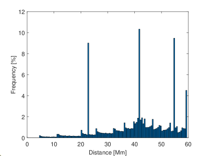
Figure 1: Histogram of pair-wise distances between Galileo satellites. The peaks indicate constant distances between satellites in the same orbital plane.

The first satellites of the present Galileo constellation were launched on October 21, 2011. Today, 26 satellites are in orbit, among them two unusable -– one with technical problems, one declared as spare due to issues with clocks –- and two on non-nominal orbits due to launch failure of the third rocket stage but otherwise fully operational and usable. In December 2016, Initial Service Declaration was announced. Currently 12 satellites, the so-called Batch 3 satellites are under production, deployment shall start in 2021. As the design lifetime of Galileo satellites is 12 years, the constellation has to be replenished in the coming years.

The Galileo constellation is a Walker constellation (Walker, 1984). This constellation type is characterized by the three numbers 24/3/1:

• Total number of satellites (i.e. eventually 24 satellites), equally distributed over the orbital planes.

• Number of equally spaced orbital planes (i.e. 3), with 8 satellites each.

• Relative spacing between satellites in adjacent planes. The difference in argument of latitude (in degrees) for equivalent satellites in neighboring planes is equal to $n_{3}*360/n_{1}$.

The revolution period corresponds to 17 revolutions in 10 sidereal days, i.e., 14h04m. With a semi-major axis of 29.600 km, the orbital inclination is 56^∘. For current Galileo satellites the eccentricity is below 0.0007 except for the two satellites on non-nominal orbits that have an eccentricity of 0.166. Fig. 1 shows the histogram of pair-wise distances between Galileo satellites in a Walker 24/3/1-constellation. Maximum distance is 59.000 km, i.e., the orbit diameter, while the mean distance is 42.000 km. The peaks in the figure indicate the constant distances between satellites in the same orbital plane.

Orbits and clock corrections for Galileo satellites are available with high precision in real time. While precise orbits at a few cm level and clock corrections at below the ns level are available in post processing, sub-meter orbits and few ns clock corrections are available through the broadcast messages that are updated every 10 minutes. While the eccentric satellites show slightly larger broadcast orbit errors, mainly in along-track, the rms of broadcast orbit errors for the other satellites is at a level of 32 cm (12.5 cm radial, 25 cm along-track, 15 cm cross-track).

In contrast, the broadcast clock quality of eccentric Galileo satellites is comparable to the other satellites. The rms of the difference is 0.50 ns. For GRB triangulation it can thus be assumed that perfect positions and time tagging are known in real time at any given time.

The attitude of the Galileo satellites is a nominal yaw steering in order to point the navigation antenna (body-fixed z-axis) to the center of the Earth and the solar panel axis (y-axis) in perpendicular direction to the direction of the Sun. The Sun is thus always located in the body-fixed x-z plane. While the positive x-surface is always illuminated by the Sun, the negative x-surface constantly points to dark sky. The nominal attitude is controlled by Earth- and Sun-sensors to below 0$.\!\!^{\circ}$1, except for non-nominal noon and midnight yaw maneuvers, if the Sun is closer to the orbital plane than about 2^∘ for IOV and about 4^∘ for FOC, and the nominal yaw rate would exceed the maximum hardware rate of 0$.\!\!^{\circ}$2/s. The negative z-axis is always pointing in zenith direction with a precision below 0$.\!\!^{\circ}$1.

4 Triangulation: methods & prospects

The triangulation method uses measurements of differences of arrival times of the same signal (GRB) at different clocks (each on a different satellite). In general, time differences between three independent satellite pairs are needed to derive a unique position on the sky, and not all these satellites shall be in the same plane.

The relation cos $\theta$ = $c{\cdot}t/d$ holds for the time difference of a signal between two satellites. Under the simplifying assumption of perfect satellite clocks and perfectly known satellite positions, the width of the annulus $\Delta\theta$ is obtained as the derivative of the above equation, i.e. is just determined by the error $\Delta t$ with which the time delay $t$ between the two signals (light curves) can be measured:

$$\Delta\theta=\left\lvert\frac{-1}{\sqrt{1-(c\cdot t/d)^{2}}}\right\rvert\Delta t\cdot\frac{c}{d}$$ (1)

There are two possible approaches to triangulation: Firstly, one can compare pairs of two light curves to each other to find the time lag, i.e. simple cross-correlation of background subtracted time series (Hurley et al., 2013; Pal’shin et al., 2013). Each satellite pair results in one time lag, and a corresponding triangulation ring. Combining multiple ($>$3) pairs then provides a unique sky position as the overlap of these triangulation rings. Cross-correlation is computationally fast, but suffers from several draw-backs (Burgess et al., 2021): (i) they only work for binned light curves, at fixed binning; (ii) no mathematical method exists to estimate the proper error of the cross-correlation; (iii) the approximation of $\chi^{2}$ rarely holds, in particular when small bin sizes are choosen in order to “increase” the temporal accuracy; (iv) the subtraction of two Poisson rates results in Skellam rather than Poisson distributed data, often leading to over-confidence; (v) it cannot take into account lightcurves taken at different energies. As a second approach, one can forward-fold an identical model through the (different) response of each detector and fit each observed light curve (Burgess et al., 2021). This technique is computationally expensive, but offers the major advantage that it produces a complete posterior probability distribution allowing for a very precise estimate of the uncertainty formally in $\Delta\theta$, but due to the forward-folding directly in sky coordinates $\Delta$RA, $\Delta$Decl. This nazgul code (Burgess et al., 2021) has been made publicly available.

5 Simulation set-up

In order to test each of the localization methods and verify their performance for different satellite configurations, we have developed a simulation framework utilizing the Python package PyIPN. This package allows for the generation of synthetic GRB light curves as seen by detectors distributed within the solar systems. We have added on top of this frame work a procedure to generate realistic light curve shapes and detector configurations that mimic the orbit of the Galileo constellation. Below we detail the setup and procedure for the generation of mock data sets which allow us to test our methods.

5.1 Simulating GRB light curves

The simulation of the triangulation capability of a network of GRB detectors requires to create mock GRB light curves which then hit differently-oriented detectors. These mock light curves shall cover a peak flux range as bright as has been seen with previous experiments (CGRO/BATSE, Swift/BAT, Fermi/GBM), and down to our proposed sensitivity limit of 1x10^-7 erg/cm²/s in the 25–150 keV band. We pick the 256 ms timescale for the peak flux as a compromise between being short enough to cover spikes in short-duration GRBs, and being general enough also for long-duration GRBs.

GRB light curves are generally very complex, and unique for each GRB. In many cases the variability time-scale is significantly shorter than the overall burst duration. Only in a minority of GRB lightcurves there is only one peak, with no substructure. The most straightforward way is to “assemble” GRB light curves by the superposition of different pulses. We assume that candidate pulses can be modeled with the empirical functional pulse form of Norris et al. (1996, 2005):

$$I(t)=A\lambda{\rm e}^{-\tau_{1}/(t-t_{s})-(t-t_{s})/\tau_{2}}{\rm cts/s}$$ (2)

where $t$ is time since trigger, $A$ is the pulse amplitude, $t_{s}$ is the pulse start time, $\tau_{1}$ and $\tau_{2}$ are characteristics of the pulse rise and pulse decay, and the constant $\lambda={\rm e}^{2(\tau_{1}/\tau_{2})^{1/2}}$. The pulse peak time occurs at time $\tau_{peak}=t_{s}+\sqrt{(}\tau_{1}\tau_{2})$. Typically, the rise times in individual GRBs are very short (steep rise), and decay times substantially longer in most times. Thus, for single-pulse GRBs, the decay time $\tau_{2}$ scales with the T90 duration of a GRB.

In order to implement the stochastic nature of the light emission process, and to incorporate unavoidable background at the measurement process, individual photon events are sampled according to an inhomogeneous-Poisson distribution following the intrinsic pulse shape specified. The photon arrival times are sampled via an inverse cumulative distribution function rejection sampling scheme (Rubinstein & Kroese, 2016). As the rate for the signal evolves with time, a further rejection sampling step is implemented that thins the arrival times according to the evolving light curve. This is done by first sampling a waiting time $t$ and computing the light curve intensity $I(t)$. Another draw from $p\in\{0,1\}$ is made and the sample is accepted if $p$ $\mathrel{\hbox{\raise 2.15277pt\hbox{$<$}\hbox to0.0pt{\hss\lower 2.15277pt\hbox{$\sim$}}}}$ $I(t)$ (Burgess et al., 2021).

The cross-correlation of two light curves depends crucially on the intensity of the GRB above background, and the structure of the light curves. We therefore need a sample of different light curves. In order to create a realistic sample, we need to make sure that we reproduce

• a rough –3/2 logN-logS intensity distribution between the brightest GRBs seen so far (2$\times$10^-4 erg/cm²/s) and our aimed-at limit of 1x10^-7 erg/cm²/s: For a canonical GRB spectrum below E_peak, i.e. a power law spectrum with a slope in the range of -0.9…-1.1 (long) and 0.0…-0.2 (hard), the following conversion holds for the 25–-150 keV band with an detector size of 3600 cm² (see below): 1$\times$10^-7 erg/cm²/s = 0.65$\pm$0.10 ph/cm²/s. Thus, we substitute the sampling over the 2$\times$10^-4 — 1x10^-7 erg/cm²/s range by that over 1300 — 0.65 ph/cm²/s.

• the observed T90 duration distribution of GRBs (Kouveliotou et al., 1993); and

• some realistic distribution between single- and multi-pulse light curve structure: We assemble multi-pulse light curves by overlapping multiple single pulses, each with a shape a la Norris et al. (1996), but with different parameters and properly delayed to each other.

For the latter, we implement a pulse avalanche, a linear Markov process, as proposed by Stern & Svensson (1996), and described in detail in appendix A. Example light curves with this simulation set-up are shown in Fig. 2.

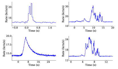
Figure 2: Example mock light curves of the long-duration class created with the pulse avalanche description of Norris-like pulses.

Energy dependent effects in GRB light curves are ignored. Conceptually, we treat our proposed energy band of 25–150 keV as a mono-energetic band.

5.1.1 Lightcurve detectability by different detectors

The previous steps provide theoretical light curves of GRBs (as emitted) which are representative in intensity distribution, duration distribution and pulse structure to the GRBs as measured over the last 30 years. These light curves are now being measured by identical detectors on a number of Galileo satellites. While the details of the Galileo satellite network is described later, three effects combine together to establish the measured light curves: (1) since the detectors are oriented into different directions, each will detect photons according to the cosine between the scintillator normal (we adopt thin, but large-area scintillator plates as baseline) and the GRB, and (2) the detector will measure quasi-isotropic $\gamma$-ray background which has the effect of washing out low-intensity features; (3) in the case of multiple detector plates per satellite, the sensitivity can be improved by co-adding the data. However, this helps only for a certain incidence angle range, since the GRB signal varies with the incidence angle, but the isotropic background does not.

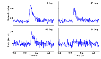
Figure 3: Light curves of the same GRB as seen with a flat detector plate from different incidence angles. The labels in each plot denote the angle under which the GRB impinges on the detector plane. With increasing angle, the effective area shrinks with the cosine of the angle, while the background remains the same. The “mother” lightcurve of this GRB has been generated with the above described pulse avalanche scheme.

An example of such a set of ’measured’ light curves for a given GRB and differently-oriented detectors is given in Fig. 3. These are the final ’measured’ light curves (in counts/s) over a certain duration in the 25–150 keV band, which are then used for triangulation.

5.1.2 Implementation of the discrete correlation function

A modified version of the discrete correlation function method (Edelson & Krolik, 1988) has been implemented in PyIPN with the following three parts: First, the model is initialized by setting a GRB position and define all detectors. The actual simulation creates the GRB signal (light curve) and computes the arrival times at the detectors as detailed above.

The final step performs the cross-correlation and computes the center point and opening angle of the circle for a specified pair of detectors. Rather than relying on mathematical covariance matrix estimation of uncertainty, cross-correlation methods heuristically derive uncertainties in one of two ways. First, the discretized time bins of the light curve yield discrete estimates of the time lag between each pair of light curves. For each value, a pseudo-$\chi^{2}$ statistics is derived yielding a grid of statistics values hopefully in a parabolic shape. The minimum of these values is taken as the true time lag (best fit). The 1, 2, and 3 $\sigma$ uncertainty regions are recovered by moving up the grid of statistics at the appropriate levels and reading off the implied time lags. This has several drawbacks: first, the best-fit time lag can never be below the timing resolution of the light curve. Additionally, the uncertainties are locked to the resolution of the grid and can thus easily be over- or under-estimated. To get around this, another heuristic can be introduced. One can fit this grid of uncertainties with a parabolic shape to effectively interpolate to finer timing resolution. While this alleviates the issues with discretization in the previous method, it introduces the problem that the interpolation has an associated uncertainty which is not accounted for. Moreover, the chosen shape of this parabolic fit cannot incorporate asymmetries in the grid and thus can easily over- or underestimate the true uncertainty. However, given the lack of a mathematically strict method, we use this procedure, but keep the problems in mind.

5.2 Gamma-ray background in the Galileo orbit

The background which a $\gamma$-ray detector (whether scintillation detector or other type) experiences in space is composed of several different components (e.g. Weidenspointner et al., 2003, 2005; Wunderer et al., 2006; Cumani et al., 2019). In the 10–250 keV band, the most important components are the extragalactic diffuse $\gamma$-ray background, Earth albedo photons (for LEO), Galactic cosmic-ray protons, and radioactive decay of activated detector and spacecraft material due to cosmic-ray bombardment. For a satellite in MEO, the diffuse $\gamma$-ray background dominates below 100 keV, while at $\sim$200 keV the rising proton contribution has reached the level of the diffuse $\gamma$-ray background. We therefore just incorporate the extragalactic diffuse $\gamma$-ray background in our simulations.

We adopt the following smoothly broken powerlaw for the diffuse background spectrum (Ajello et al., 2008):

$$E^{2}{dN\over dE}=E^{2}\times{C\over(E/E_{\rm B})^{\Gamma_{1}}+E/E_{\rm B})^{\Gamma_{2}}}$$ (3)

with the following constants: C = 0.102$\pm$0.008 ${\rm ph\ cm^{-2}\ s^{-1}\ sr^{-1}\ keV^{-1}}$, $\Gamma_{1}=-1.32\pm 0.02$, $\Gamma_{2}=-2.88\pm 0.02$ and a break at $E_{\rm B}=30.0\pm 1.1$ keV. Integrating over the 25–150 keV energy range and the 2$\pi$ sky coverage is consistent with both, the Konus-Wind (Aptekar et al., 1995) as well as Fermi/GBM (Burgess et al., 2018) measurements, and leads to $\approx$4 cts cm^-2 s^-1. This background rate is then added to the scaled light curve generated with the pulse avalanche method (see previous subsection).

5.3 Required detector timing

With a dedicated GRB detector on the Galileo satellites, we can dramatically improve the localization accuracy. Using the formal triangulation error (see eq. (1)), it is easy to compute the required temporal resolution, usually the bin size in the classical scheme, for a perfect system with satellites at known distances. Fig. 4 shows that sub-ms accuracy in the determination of the time delay is required to reach sub-degree localisation accuracy with two satellites at a distance of 42000 km (which corresponds to the mean for Galileo’s Walker constellation; see Fig. 1).

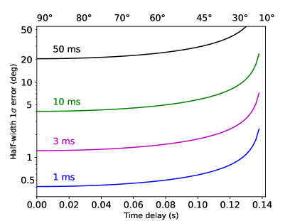
Figure 4: The 1$\sigma$ half-width error $\Delta\theta$ of the triangulation annulus is shown for a signal (GRB) arriving at a pair of satellites 42000 km apart (corresponding to the mean of Fig. 1), with different delay times (bottom x-axis label) or angles relative to the line connecting the two satellites (top x-axis) for different accuracies $\Delta t$ of 1 ms, 3 ms, 10 ms and 50 ms with which the time delay can be measured. For comparison, the Anti-Coincidence system of the INTEGRAL spectrometer (SPI-ACS) has a time resolution of 50 ms, and the shortest binning of Fermi-GBM is 64 ms, with individual events time-tagged at 2 $\mu$s.

Fig. 4 only applies for a perfect system. As discussed below, the classical triangulation method with its use of a cross-correlation of binned data sets does not provide a mathematically self-consistent error handling. In contrast, the alternative method by Burgess et al. (2020) does, but lacks the beauty of a simple equation. We therefore will show with simulations below how close this new method gets to the estimate of eq. (1).

5.4 Required detector sensitivity

Good timing resolution provides a necessary but not yet sufficient condition. The detector needs to (i) be large enough to detect a significant signal at these short time scales, (ii) measure a significant signal independent on the arrival direction, and (iii) provide this high time-resolution data for analysis, either on-board or on the ground, rather than binning it up to save telemetry band width.

A simple estimate of the minimum detector size can be made by recognizing that short-duration GRBs have structure, and do have durations substantially longer than the 3 ms time scale which Fig. 4 implies as a requirement for sub-degree localization accuracy. Assuming a canonical shape of a short GRB prompt emission lightcurve, and knowing that for GRB 170817A a single Fermi/GBM detector measured 20–30 cts/0.1 s in the 20–500 keV band at peak against $\sim$30 cts rms from background fluctuations, we estimate to need 2000 cts per short-duration (2 s) GRB or 10 cts/1 ms at peak, so $\sim$30x the effective area of a single GBM detector of 125 cm², that is 3500–4000 cm². Incorporating the correspondingly higher background rate at the Galileo orbit wrt. the LEO of Fermi will modify this estimate, but for the simulations presented here, we consider a detector of 60 cm x 60 cm geometrical area.

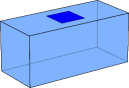
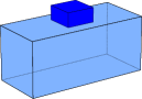
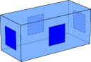
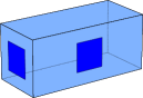
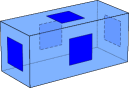
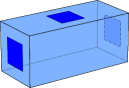
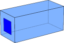
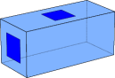
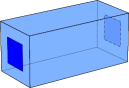
Figure 5: The different detector geometries simulated here, detector numbers 1–3 (top row) to 7–9 (bottom row).

5.5 Detector geometry

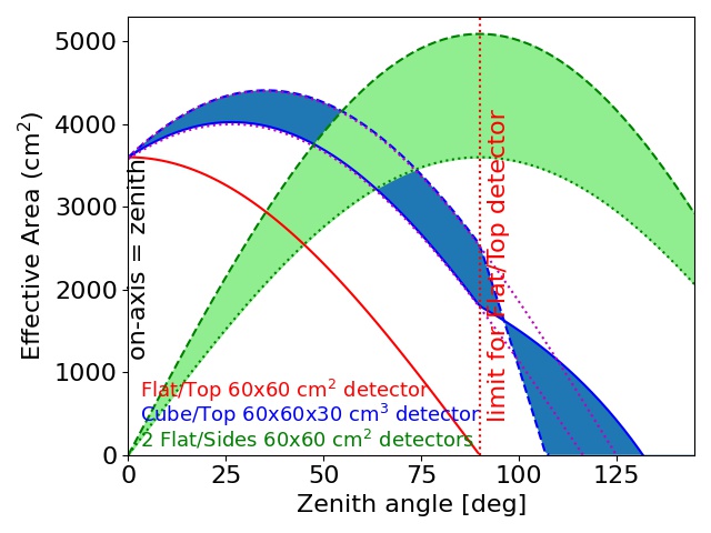
Figure 6: Off-axis dependence of the different detector geometries. The blue shaded range corresponds to the min-max range according to azimuth angle for the cube detector. Beyond 90^∘, the cube detector offers continued effective area, but shadowing by the satellite bus leads to a rapid drop. The green shaded area corresponds to equal-size detectors on two neighboring sides, with the top boundary corresponding to 45^∘ view onto both, and the lower to 90^∘ on only one of the two detectors.

As we will show, the generally preferred and assumed zenith-looking detector is not a good choice. Since the best localisation accuracy is reached at largest satellite separation and looking perpendicular to the satellite-connecting line (see eq. (1) and Fig. 4), detectors sensitive sidewards, i.e. 90^∘ of zenith, are preferred.

Since the anticipated detector size has $\approx$60 cm sidelength, adding a cube of that size to the zenith-facing side of the Galileo satellite might be challenging in terms of satellite momentum balance or station keeping, thus we also consider configurations, where one-dimensional detector plates are mounted on different sides of the Galileo satellite (Fig. 5). Any such 3D detector has several advantages: (i) multiple detector units provide independent measurements to be used in the cross-correlation; (ii) for the same reason, a coincidence veto against particle hits can be implemented, reducing the rate of false triggers; (iii) since 3D detectors cover a field-of-view (FOV) of more than 2$\pi$ of the sky, detectors on some ’behind-the-Earth’ Galileo satellites will be able to detect the GRB, thus increasing not only the number of measuring detectors, but more crucially extending the baseline (maximum distance between detectors) for the time delay measurement.

We consider nine different detector geometries (Fig. 5): a single detector facing zenith (called detector 01), a hollow cube detector with 30 cm height on the zenith-facing side (detector 02), 4 detector plates looking sideways (03), 2 neighboring sideways (+X, +Y) looking plates (04), 4 sideways plus a zenith-looking detector (05), 2 oppositely sideways and 1 zenith-looking (+X, -X; 06), 1 sideway only (+X; 07), 1 sideway plus 1 zenith-looking (+X; 08), and 2 oppositely sideways looking detectors (+X, -X; 09).

All the side-looking plates have also 60 cm $\times$ 60 cm dimension and 1 cm thickness. These configurations obviously change the zenith-angle dependent variation of the effective area; see Fig. 6: the green area corresponds to two equal-size detectors on two neighboring sides (Fig. 5). Two-dimensional versions of theses dependencies (including azimuthal variation) are shown in Fig. 11 further below.

5.6 Set-up of GNSS configuration

Since we use an existing satellite network, only one further configuration choice needs to be considered in the simulations, namely the number of satellites per orbital plane that shall be equipped with GRB detectors to allow a $4\pi$-coverage of the sky. We use the notation of [1] or [0] if a GRB detector is placed on a given satellite or not. With 8 satellites per orbital plane, and dealing with these planes consecutively, a configuration of every second satellite equipped with a GRB detector would read [10101010 10101010 10101010]. The set of simulated configurations is given in Tab. 2.

Table 2: Overview on the simulated detector configurations

Sat	Configuration	Detectors
24	11111111 11111111 11111111	1,2,3,4,5,6,7,8,9
12	10101010 10101010 10101010	1,2,3,4,5,6
9	10010010 10010010 10010010	3,5
	10010010 01001001 10100100	3,5
6	10001000 00100010 10001000	3,5
	10001000 10001000 10001000	3,5
	10010000 00010010 10010000	3,5

We compute two maps: one ’instantaneous’ snapshot map, and one averaged over one orbital period. Simulations are done in steps of 5^∘, which provides 72 subsequent snapshots for a full 14h04m orbital revolution of the Galileo satellite network, i.e. the averaged map is the average of such 72 snapshots. GRBs are distributed on the sky on a 2^∘ grid, thus providing a full sky map for each snapshot.

In order to allow any arbitrary combination of Galileo satellites to be picked, a simulation tool has been set-up (Rott, 2020) which allows to switch on/off single Galileo satellites/detectors. This is implemented as a MATLAB function galileo_skyCoverage.m, which computes the sky coverage of any Galileo constellation and a (or several) given off-axis detector response(s) (Fig. 7).

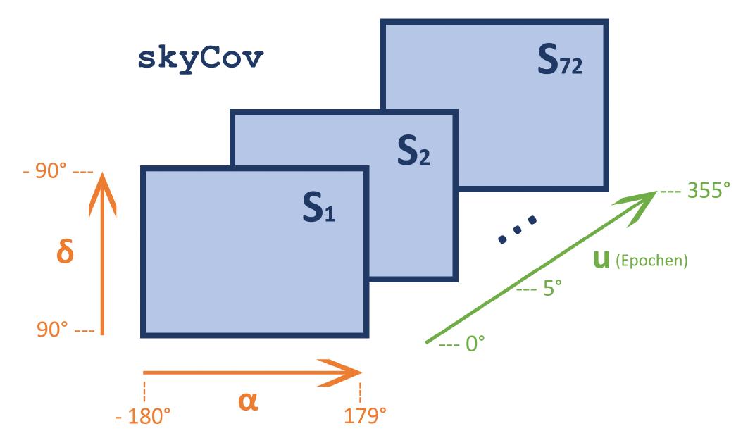
Figure 7: Structure of the skycov tensor, i.e. sky maps for the combinations of constellations and off-axis angle response. For this example, a step size (time step) of 5^∘ is assumed, resulting in 360/5=72 sky maps.

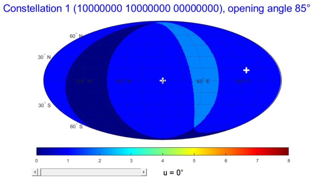
Figure 8: Example of an interactive plot for the sky coverage achieved with two Galileo satellites in separate planes, equipped with a flat GRB detector. The slide bar moves through the 72 epochs at 5^∘ steps.

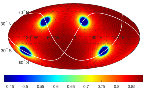
Figure 9: Mean sky coverage, i.e. the sum of 72 epochs similar to Fig. 8. Only 50% coverage is achieved at the two poles of each of the two orbital planes in which the detectors move.

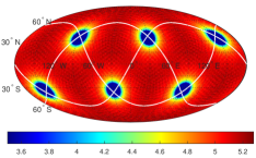
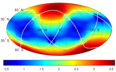
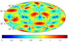
Figure 10: An extreme example of the influence of the distribution of GRB detectors over the orbital plane, with Top: the identical mean sky coverage, ranging between 3.5 and $\sim$5.3; Middle: all 12 detectors distributed over one pole, and Bottom: all 12 equally distributed. The lower two panels show the standard deviation for each point on the sky.

An example is shown in Fig. 8 for a flat GRB detector on two Galileo satellites in separate orbital planes, for one single snapshot of the constellation. Dark blue shows sky area not covered, light blue the sky covered by both detectors. Summing over one 14h04m period, i.e. 72 snapshots with 5^∘ rotation steps, results in Fig. 9, showing the mean sky coverage by two satellites.

We note that the distribution of detectors over the satellites in a given orbital plane, or also between orbital planes, has a substantial impact on the results. As a demonstration of the effect Fig. 10 shows two different constellations with the same number of satellites (with a GRB detector) per orbital plane, but grossly different distribution: (1) one with equal distribution, i.e. every second satellite has a GRB detector, and (2) all 4 satellites (with GRB detector) per orbital plane are centered over one pole of the Earth at the start configuration (epoch one out of the 72 epochs). The top panel shows the total coverage after 14h04m, which obviously is equal for both options, as it depends just on the number of satellites. The other two panels show the mean variance of the coverage at any sky position. In the equal distribution, there is no point on the sky which is covered by less than 5 and more than 6 satellites, while in the one-sphere constellation large regions of the sky are covered only with 1–2 satellites at a given time, with the consequence that triangulation would not be possible with this total number of satellites.

Since the Earth is not infinitely small, there is a 5% chance that one Galileo satellite is Earth-occulted at any given time. This is included in our computations.

6 Simulations

The simulations involve multiple steps:

1. define different detector geometries (sect. 5.5)

2. define the number of satellites and which satellites per orbital plane are equipped (sect. 5.6)

3. compute the effective area per detector configuration (sect. 6.1.1)

4. compute the accuracy of the localisation via classical cross-correlation, depending on the effective areas of the detectors on separate satellites (sect. 6.1.2)

5. simulate the sky coverage and the GRB localisation accuracy (sect. 6.1.3)

In order to cover the range of GRB peak intensities (amplitude $A$ in eq. 2) four intensity intervals are created such that faint intensity levels can be differentiated, see Tab. 3.

Table 3: Four GRB intensity intervals

Intensity ID	Peak count rate	Peak flux bin
	(ph/cm2/s)	(10-7 erg/cm2/s)
1	1.5–2	2.3–3.0
2	2–3	3.0–4.6
3	3–6	4.6–9.2
4	6–100	9.2–154

We fix the detector temporal resolution at 3 ms. Finally, we use the present 24/3/1 walker configuration of the GNSS system, and assume that satellites in all three orbital planes are indeed equipped with a detector.

These simulations return sky maps which are used to

• verify the extent to which 4$\pi$ coverage is possible with a homogeneous localisation accuracy over the sky

• verify the extent to which 4$\pi$ coverage is possible with a homogeneous flux sensitivity level

• show the differences in sky coverage and localisation accuracy as a function of different number of satellites to be equipped with a detector and the detector geometry

• provide absolute values of the GRB localisation accuracy (distribution) for both, single snapshots as well as time-averaged over the GNSS orbital period of 14h04m.

Given the CPU-intensive forward-folding triangulation technique, the full range of parameter testing in the simulation is done by using the classical cross-correlation. Only one individual set-up is computed with the forward-folding triangulation technique in order to obtain proper error estimates and compare the absolute values of GRB location accuracy (distribution). Note that in this case the above steps (3) and (4) are not necessary, since this is part of the model forward-folding.

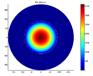
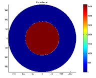
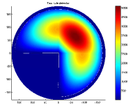
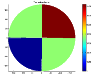
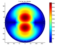
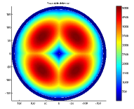
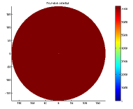
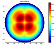
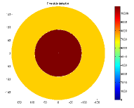
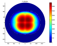
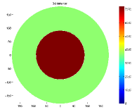
Figure 11: Two-dimensional variation of the effective area (left column) and the illuminated area (right) for our proposed geometries (each detector is 60cm x 60cm). Top row: Flat detector, zenith looking. 2nd: Two detectors on two neighboring satellite surfaces. 3rd: Two detectors on opposite sides and zenith. 4th: Four detectors on each side of the satellite, none towards zenith. The Earth shadow is included. 5th: Five detectors, one on each side and one zenith pointing. Last row: A zenith-looking cube with 30 cm height; shadowing included.

6.1 Classical scheme using cross-correlation

6.1.1 Look-up table for direction-dependent effective area

Depending on the placement of single-plate detectors on different sides of a Galileo satellite, the three-dimensional distribution of the effective area is grossly different. For illustration, we show these in Fig. 11: the left panels show the effective area as a function of azimuth and zenith angle between 0^∘ (figure center) to 180^∘ (border of figure) of an illuminating source (GRB). The right panel shows the corresponding area of the detectors that are illuminated, i.e., the area relevant for the noise. This is different from the left column figures, since the measured GRB counts per detector scale with the cosine of the incidence angle, while the background (noise) is isotropic.

The corresponding 360x180 degree matrices are used as detector-lookup tables to identify the effective area for a given illumination direction. The effective areas obtained in this way from the two detectors of a baseline are used to access the lookup-table of the accuracy matrix, see next sub-section. With both together, the different Galileo detector-equipment constellations are computed.

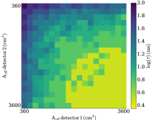
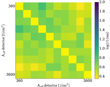
Figure 12: Distribution of the error of the time-delay (color coded) for different angles of two detectors (x- and y-axis) at the same position (=satellite), (so the nominal time delay should be zero). The matrices shown are the median of all simulated GRBs in the bright fluence bin (#4 in Tab. 3), separately computed for the classical cross-correlation method (top) and the forward-folding nazgul method (bottom), and we have separate matrices for the other intensity bins. For identical effective areas, i.e. the diagonal, nazgul recovers the nominal time delay of zero, so it was set to 0.3 to avoid division by zero in the follow-up steps. The placement on the same satellite mimics (along the diagonal) also the net effect on the accuracy of two identical detectors on different satellites looking exactly towards the same sky location. Each pixel is the median of the time-delay of many different GRB light curves. The time resolution of the detector is assumed to be 3 ms. The effective area distribution mimics a 1D detector with 3600 cm² seen at different off-axis angles.

6.1.2 Accuracy matrix

For the computation of the effects of the relative orientations of different detectors on different Galileo satellites according to the given satellite equipment scheme, we need to map the effect of detector-related parameters on the localisation accuracy in a way that they can be efficiently used. Since this localisation quality depends at least on two angles (the relative orientation of the detector normals of 2 detectors relative to the GRB direction) and the total intensity, this is a matrix rather than a factor. It is straightforward to realize that the cosine off-axis dependence of the detector sensitivity is a similar geometrical effect as different detector geometries. Thus, instead of computing effective area matrices per angle pair, we can incorporate the detector geometry (in terms of total effective area per direction) and compute the error of a delay measurement per angle pair. Such an “accuracy matrix” has been computed via both methods (Fig. 12), and then serves as input to the Galileo satellite mapping simulation.

6.1.3 Results with different detectors

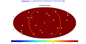
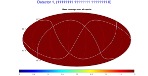
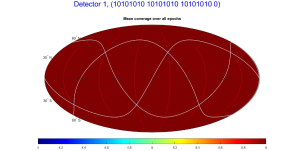
Figure 13: Sky coverage for a zenith-looking detector each on 24 (top) and 12 satellites (bottom; every second along each orbital plane) for an instantaneous moment (left) and averaged over one orbit (right). The color-coding (note the different scales) gives the number of satellites which see a GRB depending on where the GRB happens on the sky.

Detector 1: zenith-looking

We start with a single detector plate, looking at zenith, with every as well as every second of the 24 Galileo satellites equipped with one such detector. We will use this constellation to show the different aspects of the simulated data – for the other detector geometries we will primarily show example distributions and summarize the results in a table.

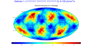
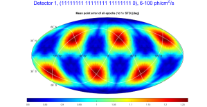
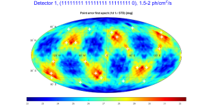
Figure 14: Localisation accuracy for a zenith-looking detector each on 24 satellites for an instantaneous moment (left) and averaged over one orbit (right), for GRBs in the brightest peak flux bin of 6–100 ph/cm²/s (top row) and the faintest peak flux bin of 1.5–2 ph/cm²/s (bottom row).

Fig. 13 shows the sky coverage for an instantaneous moment (left) and averaged over the orbit (right) for the 24- and 12-satellite options, and Figs. 14, 15 show the localisation accuracy for two different GRB flux intervals.

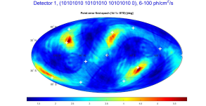
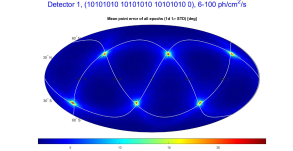
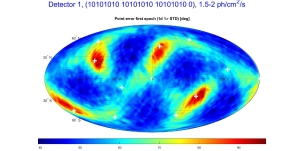
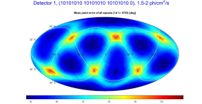
Figure 15: Same as Fig. 14 but for 12 satellites (every second along each orbital plane).

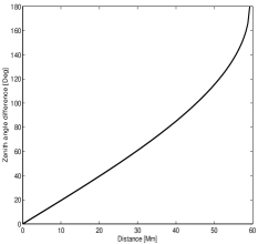
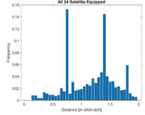
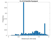
Figure 16: Left: Relation between distance between Galileo satellites and zenith pointing difference. Middle: Frequency of occurrence of satellite distances, averaged over one orbital cycle for an isotropic GRB distribution, if all Galileo satellites are equipped with a GRB detector. Right: Same, but for every second Galileo satellite equipped with a GRB detector.

For the simple 1D detector plate facing to zenith, the geometry of the satellite kinematics leads to a relation between the distance of Galileo satellites and the difference of their zenith pointing direction, as shown in the left panel of Fig. 16: The larger the angle, the lower the area in the sky that the GRB detectors on the two satellites jointly observe. More importantly, since the sensitivity of triangulation is best for GRBs occurring perpendicular to the connecting line of two satellites, zenith-looking flat detectors will not make use of the maximum baseline of the Galileo satellite system, but use at most 2/3 of it ($<$1.3 orbital radii). Our simulations over a full orbital cycle now return the frequency of occurrence of these distances between pairs of Galileo satellites for an isotropic distribution of GRBs. This shows that for the maximum GRB-detector equipment rate on the GNSS, i.e. a GRB detector on each of the 24 Galileo satellites, about half of the detector pairs occur at satellite separations of $<$1.2 orbital radii (middle panel of Fig. 16). When reducing the satellite equipment rate, this rate gets even worse (right panel of Fig. 16). Thus, a single zenith-facing detector per satellite is far from optimal.

Overview of all detector geometries

Before elucidating the details of the other detector configurations, we start with comparing the nine different GRB detector geometries by using the maximum equipment rate, i.e. all 24 Galileo satellites carry a GRB detector, in Fig. 17: the sky coverage for any given moment (left column), the average of the sky coverage over one Galileo orbital period (middle), and the mean localisation accuracy of the faintest GRB intensity bin (which is the one where our goal is to obtain a sub-degree localisation).

One interesting pattern (Fig. 17) are the green filled circles on brown sky background in the left column for detectors #03, #05, #06, and #09. These detectors all cover the whole sky (ignoring the cosine dependence of the effective area), see right column of Fig. 11. The green circles reduce the coverage by one, namely due to the shadowing of the Earth in nadir-direction, with a 12^∘ radius. Due to the three orbital planes being perpendicular to each other, there are six positions in the sky where two satellites from two orbital planes get close to each other, and their 12^∘ radii overlap to form a small region where the coverage is reduced by two satellites (blue regions).

Another aspect is symmetry: While a single detector looking towards zenith on all 24 satellites produces a homogeneous sky coverage, this is not true anymore for a single sidewards looking detector (#07, #08) or an asymmetrical detector (#04): given the Sun-pointing constraints of the Galileo system, their sky coverage is very asymmetrical.

In the following sub-sections, we describe most of these configurations in more detail.

Detector 2

As a consequence of the average short baselines for a flat, zenith-facing detector (Fig. 16), we next test a cube detector on the zenith-facing side of the Galileo satellites: these have the same area as Detector 01 towards zenith, and half of this (due to the height of only 30 cm) towards all four sides. With more satellites at large baselines and large effective area available for large parts of the sky, this substantially improves the localisation accuracy of the zenith-looking flat detector (see Figs. 18, 19).

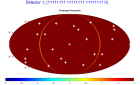
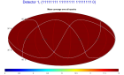
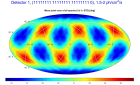
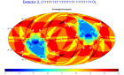
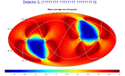
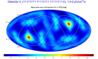
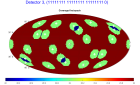
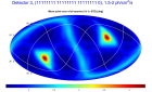
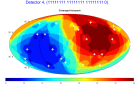
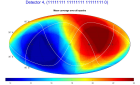
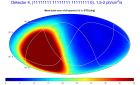
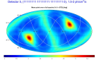
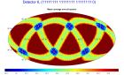
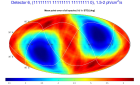
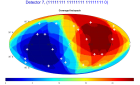
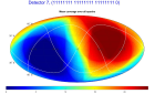
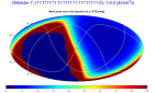
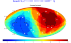
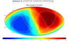
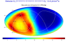
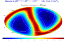
Figure 17: Sky coverage for a single time slice (left), averaged over one Galileo orbit (middle) and the averaged localisation accuracy for the faintest GRB intensity bin (right) for detector geometries 1–9 (from top to bottom) – see also blue labels for each map.

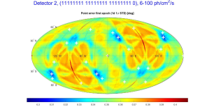
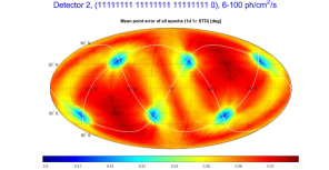
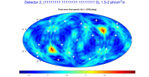
Figure 18: Localisation accuracy for a zenith-looking cube detector each on 24 satellites for an instantaneous moment (left) and averaged over one orbit (right), for GRBs in the brightest peak flux bin of 6–100 ph/cm²/s (top row) and the faintest peak flux bin of 1.5–2 ph/cm²/s (bottom row).

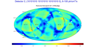
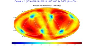
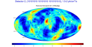
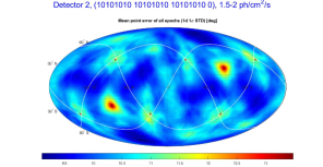
Figure 19: Same as Fig. 18 but for 12 satellites (every second along each orbital plane).

Fig. 20 illustrates why the cube detector is so much better in performance: the distribution of the mean baselines which are realized for given pairs of detectors and their projected effective areas as determined by their viewing direction relative to a GRB shows that the long baselines for higher effective areas dominate clearly. Thus, we reach sub-degree localisation accuracy for the brightest GRB intensity bin (though for the faintest it is still of order 10^∘).

Detector 3

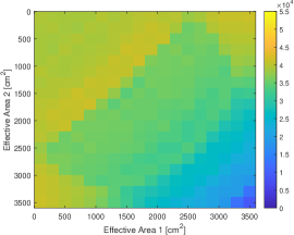
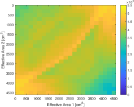
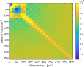
Figure 20: Distribution of mean baseline lengths for combinations of effective areas for pairs of detectors seeing a GRB for the geometries of detector #01 (left) and #02 (middle), and #03 (right).

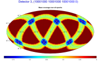
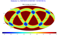
Figure 21: Sky coverage for 4-side detectors on 6 (top), 9 (left and middle of bottom row) and 12 (lower right) satellites averaged over one orbit (right). Note the different distribution of satellites along each orbital plane, with 3 different options for the 6 satellites, and two options for 9 satellites. The color-code provides the number of satellites which see a given GRB at a given time, averaged over one orbital period.

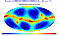
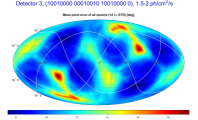
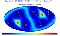
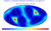
Figure 22: Localisation accuracy for a 4-side detector each on 6 (top row), 9 (lower left and middle) and 12 satellites (lower right) for the faintest intensity interval. The 6- and 9-satellite options are shown for two different configurations along the orbital plane.

With the zenith-looking detectors not being optimal, we now look at an arrangement where all 4 sides of a Galileo satellite are equipped with a 60 cm x 60 cm detector, with the nadir- and zenith-looking sides without GRB detector. The localisation accuracy is very good, see Fig. 22, even for this faintest GRB intensity level. The averaged sky coverage shows an identical sky pattern, independent of whether we equip 6, 9 or 12 satellites with a GRB detector (see Fig. 21). But note the different color-code normalization: obviously, when more satellites are equipped with a detector, then there is a larger number of satellites seeing a given GRB.

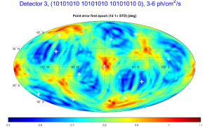
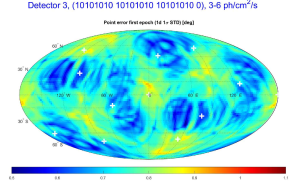
Figure 23: Localisation accuracy for a 4-side detector each on 12 satellites for the first time slice, and for the second highest intensity interval for unbinned (left) and binned (right) “accuracy matrix”, i.e. when the 6 ms binned matrix performs better than the 3 ms matrix. This happens for a certain intensity range where the increased S/N-ratio overcompensates the reduced temporal resolution of the detector. For yet fainter intensity intervals, the same happens for 9 ms, and so on. This holds for any number of satellites equipped with a GRB detector.

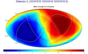
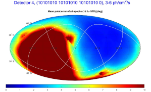
Figure 24: Sky coverage (left) and localisation accuracy (right; for the second-brightest GRB intensity interval) of 12 satellites equipped with two detector plates on neighboring sides. The sky coverage is substantially worse than any previous detector geometry.

In Fig. 23 we show the effect of the so-called ”merged” configuration, i.e. the temporal re-binning to 6 ms whenever the 3 ms sampling combined with the small baselines performs worse. This is best shown with a single time slice, not the orbit-averaged accuracy plot. The re-binning improves the bad localisation accuracy regions (red in the left panel of Fig. 23) by about 20% (from 1$.\!\!^{\circ}$1 to about 0$.\!\!^{\circ}$9).

Detector 4

With the intention to minimize the number of detector plates on a given Galileo satellite, we included this geometry with only two instead of 4 sides equipped with a 60 cm x 60 cm detector plate. The simulations show that the sky coverage is substantially worse (Fig. 24), which is a consequence of the “eyes” problem, i.e. that the detector on the y-side (together with a solar panel boom) will never look towards the Sun. In addition, as a consequence of the yaw-steering attitude, the detector mounted on the +X surface always looks into the hemisphere containing the Sun, i.e., the direction towards the anti-Sun is not covered by any detector on any satellite. The sky coverage and the localization precision thus dramatically degrade towards this direction.

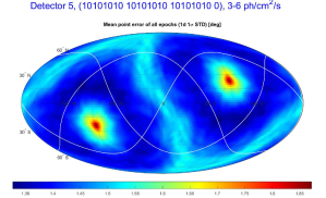
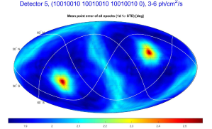
Figure 25: Localisation accuracy of 12 (left) and 9 (right) satellites equipped with 4 lateral and a zenith-looking detector, for the second brightest GRB intensity interval).

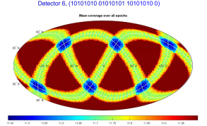
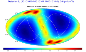
Figure 26: Sky coverage (left) and localisation accuracy (right; for the second brightest GRB intensity interval) of 12 satellites equipped with two opposite plus one zenith-looking detectors.

Detector 5

This is a kind of ’maximum detector’ concept per satellite, and unsurprisingly, the performance is very good (Fig. 25). However, we see (Tab. 4) that it performs slightly worse than the 4-lateral-only detector geometry for fainter GRB intensity levels. This is likely due to the fact that using detectors at large inclination angles towards the GRB does not help in improving the S/N-ratio, since co-adding the background noise of the second (or third) plate dominates over the gain in signal. Fig. 27 shows the effect for a single plate, and the sum of two and three perpendicular-oriented plates: at large inclination angles, i.e. small effective area due to the cosine effect, the S/N after combining detectors does not improve. This calls for an optimization of the co-adding of signals from multiple detector plates: it should not be performed on the satellite, but on the ground, as it depends on the actual noise level for each satellite (which we expect to vary along the orbit). Then, cut-off angles can be applied above which no co-addition is done. Also for this detector we find ’eyes’ in the spatial distribution of localization precision caused by the fact that maximum 2 instead of 3 of the detector plates for any satellite can cover the Sun and anti-Sun directions.

Detector 6

This three-element option, which leaves the sides with the solar panels free, eliminates the bad localization performance in Sun and anti-Sun directions (“eyes” above). However, the Sun-equator is less well covered (Fig. 26). Otherwise, it provides a very uniform localisation capability over the sky, at substantially improved accuracy as compared to the case of two neighboring detectors.

Detectors 7–9

Detectors #07, #08 and #09 were included just for completeness and verification purposes, and the results are given in the overview plot of Fig. 17.

Summary of detector geometries

Tab. 4 summarizes the different detector geometries and satellite constellations considered, providing the all-sky averaged accuracy for each of the 4 GRB intensity intervals of Tab. 3.

Thus, and quite obviously, the localisation accuracy improves with the number of satellites equipped, since among the detectors seeing a GRB, there is a larger likelihood of having satellite pairs with a large distance (baseline): only those are the ones which improve the localisation accuracy.

The placement of detectors on satellites positioned opposite to each other in the orbital plane causes moving patterns in the sky with reduced localization accuracy, and thus should be avoided; this applies primarily for low equipment rates, e.g. the 6- and 9- satellite versions discussed above.

An interesting feature is seen in the case with 6 satellites: when the GRB detectors are distributed isotropically, i.e. 2 per orbit at antipodal positions, there is a pattern on the sky at which the localisation is substantially worse (top left panel in Fig. 22). This can be avoided by placing detectors not in antipodal positions (next panel to the right in Fig. 22).

One special effect to comment on are the two “eyes” in Fig. 22 (lower row). These are due to the position of the Sun in the simulation ($\alpha$ = 90^∘, $\delta$ = 23^∘) and the anti-Sun direction, and in practice would move over the sky over the course of a year. These are caused by the yaw-steering motion of the satellite guaranteeing pointing of the navigation antenna continuously to the Earth and the solar panels to the Sun. As a consequence of this attitude mode the +Y and-Y surfaces of the satellite where the solar panel booms are mounted never look towards the Sun. The Sun and anti-Sun directions are thus covered only by one detector plate per satellite with varying orientation towards the Sun. The result is a reduced localization precision in these directions. For the GRB/GW application this is acceptable, since optical follow-up of the GRB or neutron star merger close to the Sun is anyway not possible from the ground.

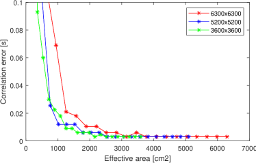
Figure 27: Accuracy of different detector configurations: As one adds perpendicular-oriented detector plates, and since the background radiation is isotropic and does not scale with the cosine of the incidence angle, the S/N-ratio depends on the relative inclination angles of the plates: it is best for a single plate (green), and gets worse for two plates inclined by 90 degrees (blue), and even worse for three plates inclined by 90 degrees (red; corresponding to the 5-detector case for any given GRB).

For obtaining the localisation accuracy in Tab. 4, we averaged over the full sky. But looking at the various figures, it becomes obvious that there are certain small (few to 10% of the sky) regions on the sky which are worse than the majority of the sky. We therefore provide a more accurate accounting of the localisation accuracy for our best options in Tab. B. This provides the worst accuracy for the best 50% and 90% of the sky (i.e. the accuracy is better than the specified value for that percentage of the sky), respectively, as well as the best and the worst single GRB accuracy of the sky. For the selected best detector and satellite configurations, we also provide a graphical representation in Fig. 28 which allows to get the accuracy for any fraction of sky coverage.

6.2 Bayesian scheme using nazgul

Due to the massive compute-time requirements, a simulation with nazgul was only done for one particular satellite constellation (9 satellites, 3 in each orbital plane, equally distributed) with one detector (#03, looking towards 4 sides). We use the same set-up as the one to reconstruct the time with the cross-correlation algorithm. Instead of 1000 different GRB light curves, we use only one light curve shape, with 5 different flux normalization. Also, the triangulation was only computed at 134 sky positions, instead of 10000. From each fit we obtain a distribution of the time delay which is used to compute both the “best” fit value (the median in this case) and the 68% probability uncertainties through the highest posterior density interval, i.e. the shortest possible interval, necessary to accumulate the chosen probability level. While the source position distribution reconstructed by nazgul is not, in general, an annulus, for the sake of a straightforward comparison with the classical correlation method we compute an “equivalent” annulus from the fitted time delay. The central ring of the annulus is computed from the median of the time delay distribution, while the width is given by the uncertainties in an analogous way as what is done for the correlation method (see, e.g., Pal’shin et al., 2013). This methodology, although to some extent simplistic, allows us to compare the characteristic widths of the positional distributions fitted by nazgul and the correlation algorithm. The corresponding ’map’ is shown in Fig. 29 for the faintest intensity interval, together with the corresponding map from the cross-correlation method. This shows, that the two methods are nicely compatible to each other.

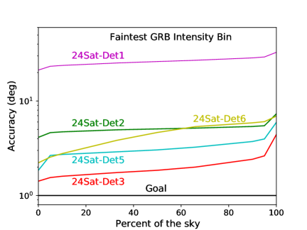
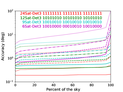
Figure 28: Accuracy of different detector and satellite configurations per sky fraction. Each curve shows the percentage of the sky for which the accuracy is better than the corresponding y-axis in degrees. Top: for the faintest intensity bin for 24 satellite equipment rate; Bottom: each color represents one configuration of Tab. B for detector #3, with solid lines for the brightest GRB interval, and dotted lines for the faintest.

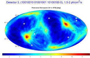
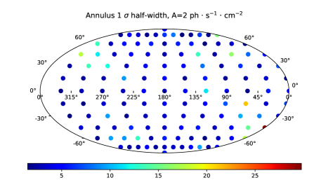
Figure 29: Localisation accuracy for detector #03 (4 sides) and 9 satellites for the first of 72 snapshot per orbital phase and the faintest GRB intensity bin, computed with cross-correlation (left) and nazgul (right). Note that the Sun is not included in the nazgul simulation, and thus the “eyes” are missing.

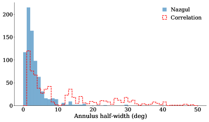
Figure 30: Distribution of the absolute value of the difference between simulated and reconstructed time delays for nazgul (blue) and the cross-correlation method (green), again for detector #03 (4 sides) and 9 satellites.

A more quantitative comparison of the localisation accuracy is given in Fig. 30, showing the histogram of the 1$\sigma$ localization errors of nazgul vs. the cross-correlation method. This shows, that the nazgul distribution is a factor $\sim$2 narrower (FWHM of about 4^∘ vs 8^∘), and has much less GRB reconstructions in the long tail. Thus, the nazgul method leads to overall improvements, but is particularly superior at the faint end of the intensity distribution.

6.3 Comparison to previous simulations

Recently, Hurley (2020) has combined a new localisation method with the simulation of a near-Earth network of GRB detectors. The basic concept of this method is similar to ours, namely avoiding cross-correlation and instead testing positions on the sky via a likelihood method. While this method is a substantial improvement over the classical cross-correlation, it still suffers from the above draw-backs (iii) and (iv) in sect. 4 which is accounted for in our nazgul scheme (Burgess et al., 2021). In his simulations, he uses individual detectors of 100 cm² effective area on a fleet of nine satellites, and derives localisation accuracies for three different GRB peak intensities. His faintest and middle intensity intervals fall in our brightest interval. In terms of sky coverage, Hurley (2020) reaches only 40%, so a single-plate detector on each of 9 satellites is by far too little to reach all-time, all-sky coverage. While we have not simulated such a constellation, this result is consistent with our picture, i.e. the need to look to multiple sides at this small satellite number. The 1$\sigma$ average localisation for his faintest fluence GRB (16 ph/cm²/s) is an ellipse with a dimension of 4$.\!\!^{\circ}$5$\times$17$.\!\!^{\circ}$0, corresponding to an effective radius (same-area circle) of 4$.\!\!^{\circ}$5 (1$\sigma$). Our closest constellation is a 1-side (zenith) looking detector on 12 satellites, where our simulation for our brightest intensity interval (6–100 ph/cm²/s) gives 2$.\!\!^{\circ}$9. The difference between these two simulations is in effective area (100 vs. 3600 cm²), orbit radius (7000 vs. 29.000 km), and timing accuracy (0.1 vs. 3 ms). Assuming the typical square-root dependence on effective area, the combination of these three factors suggests that our error should be $1/\sqrt{36}/29*7*30=1.2\times$ that of the Hurley (2020) simulation, pretty close to what we obtain (given that our intensity bin is very wide).

6.4 Potential for improvements

Given the comparison in the previous subsection, one could ask whether or not reducing the time resolution in our simulations (fixed at 3 ms) would substantially improve our localisation accuracy? The answer is: in theory yes, in practice likely not. The simple reason is that the variability time scale in GRBs is at the level of a few milliseconds (MacLachlan et al., 2013), and not sub-milliseconds (Walker et al., 2000). Thus, one needs to cross-correlate the rising edge of a pulse to better then the rise time. This is complicated even further due to the fact that the slopes of the rise are energy dependent, i.e. detectors like the here preferred scintillator plates will see different slopes from the same GRB as soon as the incidence angles on two detectors are not exactly the same. This is the reason why for instance co-adding of light curves of different GBM detectors is of no avail.

For configurations with more than one detector plate per satellite, we have co-added multiple single-plate detectors per satellite. As described earlier, this does not automatically provide better S/N-ratio, since the background radiation adds in full, not diminished with the cosine law as the source counts. Therefore, some optimization for adding two or three detector plates could be implemented. This affects mostly the faint end of the GRB intensity distribution, and the optimization is expected to improve the localization accuracy. On a practical note, the data from different detector plates should thus not be combined onboard, but send down to Earth separately. As a side effect, the onboard triggering algorithm can make use of the separate light curve measurements to filter out particle hits, thus dramatically reducing false triggers.

There is yet another way to improve the accuracy distribution, computed via the classical cross-correlation analysis, beyond what we presented: namely using systematically a re-binning procedure (in an frequentist approach, and the corresponding $\chi^{2}$ analysis). In practice, when moving from bright to fainter GRBs, there is a transition region where re-binning from the original 3 ms time resolution of the detector towards, e.g., 6 ms provides a gain over the noise fluctuations, and leads to an improved localisation. This has been shown above with our ’merged’ map for one case (Fig. 23). But moving further down in intensity, the same happens for further re-binning to 9 ms, or 12 ms, and so on. The effect of this re-binning is to optimize between noise in the light curve vs. the best accuracy in the time delay measurement. Obviously, it does not improve on the best accuracy side, but improves the bad end by of order 15%-20%. This, of course, does not apply to our forward-folding nazgul localisation, since this is Bayesian, and the information in “low S/N” bins is properly accounted for.

6.5 Inclusion of satellites beyond GNSS

The inclusion of any satellite further out in space than the Galileo satellites would help reducing the localisation accuracy, as it shrinks linearly with the increase of the baseline. Potential options are a GRB detector on (i) the Gateway, a multi-purpose space station in a highly elliptical (3000 km x 70.000 km) seven-day near-rectilinear halo orbit around the Moon, presently planned to be assembled in the 2024–2028 timeframe, or (ii) the Moon LCS (Lunar navigation and communication system), a network of 3–4 satellites that would provide communications and navigation services to support human and robotic exploration on the Moon. A GRB detector in Lunar orbit would reduce the localisation error by a factor of $\sim$6, if the GRB detector has the same size as discussed here for the GNSS. Of course, this improvement would only apply in one dimension of the error box, for GRBs coming from a direction perpendicular to the Earth-Moon line.

7 GNSS system requirements

7.1 Communication speed

The GRB afterglow brightness fades by a factor of three during the first 10 min. after the burst, another factor of three during the next 50 min., and another factor of three during the next 23 hrs. The kilonova emission of short GRBs decays even faster. Moreover, clarifying the presently hottest open astrophysics questions of merging neutron stars such as distinguishing the physical source of energy input (e.g. from the central remnant or via radioactivity) or associated processes (e.g. internal shock-reheating or heating of the outer ejecta by free neutrons) requires ground-based optical/near-infrared spectroscopy during the first 12 hrs (Metzger, 2020). Thus, rapid communication at a timescale of minutes is required in order to support the identification of the kilonova.

GRBs occur at unpredictable time and sky position. For the GRB position to be determined via triangulation, we need the measured data of each of the $>$4 satellite detectors on one computer. In order to be scientifically useful, the data should be downlinked within of order a few minutes. Thus, we require that at any time every Galileo satellite can send off its measured data, either directly or via another satellite to a ground-station. Since only 6 TT&C stations around the world are responsible for collecting and sending the telemetry data that was generated by the Galileo satellites, relaying data between different Galileo satellites to the one (or few) which do have ground contact is a viable solution. This should be done dynamically, without the need of commanding, i.e. each satellite (computer) should know at any time its acting relay satellite.

We distinguish two data transmission rates: (1) full rate to be downlinked to Earth, within minutes: for a typical GRB, this implies sending 0.5–1 MB over a time period of a few minutes, e.g. 4–8 kB/s over 2 minutes per satellite. (2) reduced rate for quick-look localisation. As described above, this would reduce the data amount by a factor of 100–1000.

The inter-satellite data transmission rate is likely slower than a satellite-ground contact rate. Assuming 4 Galileo satellites without ground-contact shall send data to one other satellite with ground-contact leads to a required transfer rate of 4 MB on a time-scale of minutes. In an ideal case, this can be done in parallel. If not, the above 4–8 kB/s are a minimum requirement.

Rapid up-link capability is not needed, since the GRB detectors should be self-triggering.

7.2 Ground segment

The light curve data as measured by the multiple Galileo satellites should be collected at one place on Earth, where the triangulation (and thus GRB localisation) can be computed. We suggest that the final localisation is made publicly available immediately – the GRB community is using the GCN (Gamma-ray Burst Coordinate Network) for this since decades, which would guarantee distribution to every interested user in the world. This would typically happen automatically, but oversight through a, or several, (GRB) astronomer(s) is certainly not a bad idea. This could be organized via forming a small group of interested scientists, similar to groups which collaborate in the follow-up observations of GRBs at optical or radio observatories. In parallel, also the raw data should be made publicly available at the shortest possible delay time, to allow other groups with potential access to other long-baseline GRB data to use those data. The high-energy mission archive at ESA would be a logical place, but other satellite data centers in Europe might be alternative options.

8 Conclusions

The GNSS provides a close-to-perfect satellite system for the localisation of gamma-ray bursts (GRBs) via triangulation. It provides a very promising compromise between satellite baselines (not too long to suffer data transmission restrictions), number of satellites, and required size of GRB detectors to reach sub-degree localizations. It is the combination of detector geometry (to how many of the six directions of the Galileo surfaces are the detectors facing) and the number of satellites to be equipped, which provides a scientifically useful GRB triangulation network.

Sideways looking detectors are an extremely crucial ingredient. We suggest to equip at least 12 satellites, four per orbital plane, with a 4-side (excluding nadir and zenith) looking detector, each side with 3600 cm² and 1 cm thickness. This will provide sub-degree localisation of GRBs, in particular faint short-duration GRBs such as GRB 170817A, as expected from binary neutron star mergers to be routinely measured at a rate of dozens per year in the upcoming runs of the worldwide gravitational wave detectors. Instead, a flat, zenith-facing detector provides only 10-20^∘ localizations. Equipping only 9 Galileo satellites with such a GRB detector leads to a 30% loss in localisation accuracy, while the 24-satellite solution improves it by a factor 2.

Such a configuration should be feasible to implement given the moderate requirements of mass ($<$20 kg) and power ($\sim$20 W) of a single detector plate (i.e. $<$80 kg and $\sim$80 W for the 4-side detector) as compared to the overall budget of a Galileo satellite, though we note that this corresponds to about 10% of the satellite mass. The realization of such a large-format GRB detector plate is also technologically feasible: scintillators of the proposed type have been flown since 40 years (TRL 9), and the Si detectors for read-out have also seen their first space applications.

Equipping second generation Galileo satellites with GRB detectors would turn the navigation constellation into an observatory supporting the research on fundamental astrophysical and cosmological problems.

Appendix A Implementation of simulated light curves

For a realistic distribution of single vs. multi-pulse light curves, we implement a pulse avalanche, a linear Markov process, as proposed by Stern & Svensson (1996). Here, each pulse acts as a parent pulse giving rise to a number of baby pulses $\mu_{b}$, sampled from a Poisson distribution $p_{2}(\mu_{b})=\mu^{-1}{\rm exp}(-\mu_{b}/\mu)$, with the average number being $\mu$. A baby pulse is assumed to be delayed by a time $\Delta$t with respect to the parent pulse. The probability distribution for the Poisson delay is parameterized as $p_{3}(\Delta t)=(\alpha\tau)^{-1}{\rm exp}(-\Delta t/\alpha\tau)$, where $\tau$ is the time constant of the baby pulse and $\alpha$ is the delay parameter. From observed GRBs, the time constant $\tau$ of baby pulses is of the same order of magnitude, but shorter than the time constant $\tau_{1}$ of the parent pulse. This allows the process to converge, since the pulse avalanche eventually reaches an arbitrary short timescale, where a natural frequency cutoff should exist. The corresponding probability distribution is considered to be uniform in log($\tau/\tau_{1}$), and parameterized as $p_{4}[{\rm log}(\tau/\tau_{1})]=\lvert\delta_{2}-\delta_{1}\rvert^{-1}$ in the range [$\delta_{1},\delta_{2}$] with $\delta_{1}<0$, $\delta_{2}$ $\mathrel{\hbox{\raise 2.15277pt\hbox{$>$}\hbox to0.0pt{\hss\lower 2.15277pt\hbox{$\sim$}}}}$ 0, and $\lvert\delta_{1}\rvert>\lvert\delta_{2}\rvert$. The number of spontaneous pulses $\mu_{s}$ is sampled from a Poisson distribution $p_{5}(\mu_{s})=\mu^{-1}{\rm exp}(-\mu_{s}/\mu_{o})$, with $\mu_{s}$ the average number of spontaneous pulses per GRB. Lastly, the probability distribution of the time constants $\tau_{0}$ of spontaneous pulses is taken as $p(\tau_{0})\propto 1/\tau_{0}$, corresponding to a 1/f flicker noise spectrum. Observations imply an maximum $\tau_{\rm max}$ for $\tau_{0}$. We then sample ${\rm log}\tau_{0}$ uniformly between $\tau_{\rm min}$ and $\tau_{\rm max}$, i.e. $p_{6}({\rm log}\tau_{0})=({\rm log}\tau_{max}-{\rm log}\tau_{\rm min})^{-1}$, where $\tau_{\rm min}$ should be smaller than the time resolution. Varying $\tau_{\rm max}$ rescales all average avalanche properties in time. Since more than one parent pulse is allowed per GRB, these spontaneous primary pulses are all assumed to be delayed with different time intervals $t$ with respect to a common invisible trigger event. We parameterize the probability distribution for the Poisson delay $t$ of a given spontaneous pulse as $p_{7}(t)=(\alpha\tau_{0})^{-1}{\rm exp}(-t/\alpha\tau_{0})$, where $\alpha$ is the constant delay parameter used for all pulses and $\tau_{0}$ is the time constant of the spontaneous pulse. Each spontaneous pulse gives rise to a pulse avalanche, and it is the overlap of $\mu_{s}$ pulse avalanches that form a GRB. From the analysis of about 600 CGRO/BATSE GRBs, Stern & Svensson (1996) suggest the following parameters: $\mu=1.2$, $\alpha=4$, $\delta_{1}=-0.5$, $\delta_{2}=0$, $\mu_{0}=1$, $\tau_{\rm max}=26$ s. Differently than Stern & Svensson (1996), we pick $\tau_{\rm min}=0.2$ s to allow for a better time resolution for the Galileo detector. We do simulate short and long GRBs separately to better tune some of the $\tau_{i}$ parameters, see example light curves in Fig. 2.

Appendix B Location accuracy

Table 4: Average localisation accuracy for different detector geometries on a differing number of satellites.

Detector geometry	No. of	Orbit configuration	Error radius
	Satellites		(1$\sigma$, deg)
			2.3–3	3–4.6	4.6–9.2	9.2–154
			(10-7 erg/cm2/s)
01 – zenith-looking	24	11111111 11111111 11111111	26.2	11.7	3.9	1.0
	12	10101010 10101010 10101010	63	31	11.0	2.9
02 – Cube at zenith	24	11111111 11111111 11111111	5.1	1.6	0.8	0.4
	12	10101010 10101010 10101010	10.3	3.2	1.6	0.7
03 – 4 lateral sides	24	11111111 11111111 11111111	1.9	0.7	0.4	0.2
	12	10101010 10101010 10101010	4.2	1.4	0.8	0.4
	9	10010010 10010010 10010010	5.4	1.8	1.0	0.5
	9	10010010 01001001 10100100	5.4	1.8	1.0	0.5
	6	10001000 10001000 10001000	12.9	4.1	2.2	1.0
	6	10001000 00100010 10001000	24.6	8.2	4.4	2.2
	6	10010000 00010010 10010000	11.0	3.5	2.0	1.0
04 – 2 neighbouring sides	24	11111111 11111111 11111111	28.2	16.2	6.5	1.9
	12	10101010 10101010 10101010	57	34.4	14.7	4.4
05 – 5 sides	24	11111111 11111111 11111111	3.2	1.1	0.5	0.2
	12	10101010 10101010 10101010	10.5	4.5	1.4	0.4
	9	10010010 10010010 10010010	14.5	6.2	2.0	0.6
	9	10010010 01001001 10100100	14.7	6.3	2.0	0.6
	6	10001000 10001000 10001000	27.9	12.2	3.8	1.1
	6	10001000 00100010 10001000	45	20.6	6.5	1.8
	6	10010000 00010010 10010000	28.2	12.1	3.7	1.0
06 – 2 opposite sides & zenith	24	11111111 11111111 11111111	4.5	1.5	0.8	0.3
	12	10101010 01010101 10101010	7.9	2.5	1.3	0.6
08 – 1 side & zenith	24	11111111 11111111 11111111	15.7	6.5	2.4	0.7
09 – 2 opposite sides	24	11111111 11111111 11111111	12.0	5.7	1.8	0.5

[x]ccccccccc Localisation accuracy for selected detector geometries according to fractional sky area. Brightness bins are according to Tab. 3, with 1 the faintest, and 4 the brightest.
Name Detector geometry No. of Orbit configuration Intens. precision $<$p[^∘] for % of sky
Sats Intvl best 50% 90% worst
continued.
Name Detector geometry No. of Orbit configuration Intens. precision $<$p[^∘] for % of sky
Sats Intvl best 50% 90% worst
01 zenith 24 11111111 11111111 11111111 1 21.3   26.2   28.6   32.8  
24 11111111 11111111 11111111 2 9.1 11.7   13.0   14.4  
24 11111111 11111111 11111111 3 2.9 3.8 4.6 5.4
24 11111111 11111111 11111111 4 0.7 1.0 1.2 1.3
01 zenith 12 10101010 10101010 10101010 1 34.5   57.2   87.8   180
12 10101010 10101010 10101010 2 17.0 26.2   47.8   180
12 10101010 10101010 10101010 3 4.8 8.6 17.9   180
12 10101010 10101010 10101010 4 1.0 2.2 4.4 180
02 cube @ zenith 24 11111111 11111111 11111111 1 4.1 5.1 5.4 7.3
24 11111111 11111111 11111111 2 1.4 1.6 1.6 2.4
24 11111111 11111111 11111111 3 0.7 0.8 0.9 1.1
24 11111111 11111111 11111111 4 0.3 0.4 0.4 0.4
02 cube @ zenith 12 10101010 10101010 10101010 1 6.9 10.1   11.9   18.2  
12 10101010 10101010 10101010 2 2.5 3.1 3.6 5.3
12 10101010 10101010 10101010 3 1.1 1.6 1.8 2.4
12 10101010 10101010 10101010 4 0.5 0.7 0.8 0.9
03 4 lateral sides 24 11111111 11111111 11111111 1 1.4 1.9 2.4 4.4
24 11111111 11111111 11111111 2 0.5 0.6 0.8 1.2
24 11111111 11111111 11111111 3 0.3 0.4 0.4 0.5
24 11111111 11111111 11111111 4 0.2 0.2 0.2 0.2
03 4 lateral sides 12 10101010 10101010 10101010 1 2.6 3.8 5.5 10.6  
12 10101010 10101010 10101010 2 1.0 1.3 1.7 2.5
12 10101010 10101010 10101010 3 0.5 0.8 0.9 1.2
12 10101010 10101010 10101010 4 0.4 0.4 0.4 0.5
03 4 lateral sides 9 10010010 10010010 10010010 1 3.2 5.0 7.0 13.8  
9 10010010 10010010 10010010 2 1.2 1.7 2.2 3.5
9 10010010 10010010 10010010 3 0.6 1.0 1.2 1.7
9 10010010 10010010 10010010 4 0.5 0.5 0.6 0.7
03 4 lateral sides 9 10010010 01001001 10100100 1 3.2 5.2 7.1 16.0  
9 10010010 01001001 10100100 2 1.1 1.8 2.2 3.6
9 10010010 01001001 10100100 3 0.6 1.0 1.2 1.6
9 10010010 01001001 10100100 4 0.5 0.5 0.6 0.7
03 4 lateral sides 9 10010010 10010010 10010010 1 3.2 5.0 7.0 13.8  
9 10010010 10010010 10010010 2 1.2 1.7 2.2 3.5
9 10010010 10010010 10010010 3 0.6 1.0 1.2 1.7
9 10010010 10010010 10010010 4 0.5 0.5 0.6 0.7
03 4 lateral sides 9 10010010 01001001 10100100 1 3.2 5.2 7.1 16.0  
9 10010010 01001001 10100100 2 1.1 1.8 2.2 3.6
9 10010010 01001001 10100100 3 0.6 1.0 1.2 1.6
9 10010010 01001001 10100100 4 0.5 0.5 0.6 0.7
03 4 lateral sides 6 10010000 00010010 10010000 1 4.2 9.7 17.5   109
6 10010000 00010010 10010000 2 1.6 3.2 5.3 39.2 
6 10010000 00010010 10010000 3 0.8 1.8 2.8 21.1 
6 10010000 00010010 10010000 4 0.7 0.9 1.3 9.6
04 2 neighbouring sides 24 11111111 11111111 11111111 1 3.5 12.2  80.5   180
24 11111111 11111111 11111111 2 1.1 4.5 41 180
24 11111111 11111111 11111111 3 0.5 1.9 11.8   180
24 11111111 11111111 11111111 4 0.2 0.6 3.0 180
04 2 neighbouring sides 12 10101010 10101010 10101010 1 6.4 27.7  180 180
12 10101010 10101010 10101010 2 2.2 11.3  109 180
12 10101010 10101010 10101010 3 0.9 4.1 32.3   180
12 10101010 10101010 10101010 4 0.4 1.1 8.1 180
05 4 sides + zenith 24 11111111 11111111 11111111 1 1.9 3.0 3.7 5.9
24 11111111 11111111 11111111 2 0.7 1.1 1.3 2.0
24 11111111 11111111 11111111 3 0.4 0.5 0.6 0.7
24 11111111 11111111 11111111 4 0.2 0.2 0.2 0.2
05 4 sides + zenith 12 10101010 10101010 10101010 1 8.3 10.3  12.1  15.7  
12 10101010 10101010 10101010 2 3.7 4.5 5.1 7.1
12 10101010 10101010 10101010 3 1.1 1.4 1.6 2.0
12 10101010 10101010 10101010 4 0.4 0.4 0.4 0.5
05 4 sides + zenith 9 10010010 10010010 10010010 1 10.1  14.3  16.8  25.0  
9 10010010 10010010 10010010 2 4.5 6.1 6.4 10.7  
9 10010010 10010010 10010010 3 1.5 1.9 2.0 2.9
9 10010010 10010010 10010010 4 0.5 0.6 0.6 0.8
05 4 sides + zenith 9 10010010 01001001 10100100 1 10.0  14.5  17.4  26.0  
9 10010010 01001001 10100100 2 4.5 6.2 7.4 11.5  
9 10010010 01001001 10100100 3 1.5 2.0 2.3 3.0
9 10010010 01001001 10100100 4 0.5 0.6 0.6 0.7
05 4 sides + zenith 6 10001000 10001000 10001000 1 13.2  23.9  38.4   180
6 10001000 10001000 10001000 2 6.0 10.2  16.5   180
6 10001000 10001000 10001000 3 1.8 3.2 5.0 180
6 10001000 10001000 10001000 4 0.6 0.9 1.4 180
05 4 sides + zenith 6 10001000 00100010 10001000 1 13.0  30.4  92.8   180
6 10001000 00100010 10001000 2 5.9 13.0  40.7   180
6 10001000 00100010 10001000 3 1.6 3.9 12.4 180
6 10001000 00100010 10001000 4 0.6 1.1 3.5 180
05 4 sides + zenith 6 10010000 00010010 10010000 1 12.0  26.2  39.5   180
6 10010000 00010010 10010000 2 5.3 11.2  16.8   110
6 10010000 00010010 10010000 3 1.7 3.9 5.2 39.8  
6 10010000 00010010 10010000 4 0.7 1.1 1.4 11.7  
06 2 opposite sides+zenith24 11111111 11111111 11111111 1 2.2 4.7 5.9 6.9
24 11111111 11111111 11111111 2 0.8 1.5 1.9 2.4
24 11111111 11111111 11111111 3 0.4 0.8 1.0 1.2
24 11111111 11111111 11111111 4 0.2 0.4 0.4 0.6
06 2 opposite sides+zenith12 10101010 01010101 10101010 1 4.5 10.5   17.4   38.4 
12 10101010 01010101 10101010 2 1.5 3.2 5.3 17.1 
12 10101010 01010101 10101010 3 0.8 1.6 2.6 9.3
12 10101010 01010101 10101010 4 0.5 0.7 1.1 6.6
07 1 side 24 11111111 11111111 11111111 1 4.0 45.6   180 180
24 11111111 11111111 11111111 2 1.8 23.8   180 180
24 11111111 11111111 11111111 3 0.7 7.0 180 180
24 11111111 11111111 11111111 4 0.2 1.8 180 180
08 1 side + zenith 24 11111111 11111111 11111111 1 2.2 14.0   29.4   39.5  
24 11111111 11111111 11111111 2 0.8 5.3 13.0   16.7  
24 11111111 11111111 11111111 3 0.4 2.3 4.5 6.2
24 11111111 11111111 11111111 4 0.2 0.7 1.2 1.6
09 2 opposite sides 24 11111111 11111111 11111111 1 4.0 10.6  21.5   24.6  
24 11111111 11111111 11111111 2 2.0 5.7 10.9  13.3  
24 11111111 11111111 11111111 3 0.7 1.5 3.3 4.3
24 11111111 11111111 11111111 4 0.2 0.4 0.8 1.2