Utterance Weighted Multi-Dilation Temporal Convolutional Networks for Monaural Speech Dereverberation

Abstract

Speech dereverberation is an important stage in many speech technology applications. Recent work in this area has been dominated by deep neural network models. TCN are deep learning models that have been proposed for sequence modelling in the task of dereverberating speech. In this work a weighted multi-dilation depthwise-separable convolution is proposed to replace standard depthwise-separable convolutions in temporal convolutional network (TCN) models. This proposed convolution enables the TCN to dynamically focus on more or less local information in its receptive field at each convolutional block in the network. It is shown that this weighted multi-dilation temporal convolutional network (WD-TCN) consistently outperforms the TCN across various model configurations and using the WD-TCN model is a more parameter-efficient method to improve the performance of the model than increasing the number of convolutional blocks. The best performance improvement over the baseline TCN is 0.55 dB SISDR and the best performing WD-TCN model attains 12.26 dB SISDR on the WHAMR dataset.

Index Terms—  speech dereverberation, temporal convolutional network, speech enhancement, receptive field, deep neural network

1 Introduction

Speech dereverberation remains an important task for robust speech processing [1, 2, 3]. Far-field speech signals such as for automatic meeting transcription and digital assistants normally require preprocessing to remove the detrimental effects of interference in the signal [4, 5, 6]. A number of methods have been proposed for speech dereverberation for both single channel and multichannel models [7]. Recent advances in speech dereverberation performance in a number of domains have been driven by deep neural network (DNN) models [8, 9, 10, 11, 12].

Convolutional neural network models are commonly used for sequence modelling in speech dereverberation tasks [13, 14, 15]. One such fully convolutional model known as the TCN has been proposed for a number of speech enhancement tasks [16, 17, 18]. TCN are capable of monaural speech dereverberation as well as more complex tasks such as joint speech dereverberation and speech separation [17]. The best performing TCN models for speech dereverberation tasks typically have a larger receptive field for data with higher reverberation times T60 and a smaller receptive field for data with small T60s [19] which forms the motivation for this paper.

In this work, a novel TCN architecture is proposed which is able to focus on specific temporal context within its receptive field. This is achieved by using an additional depthwise convolution kernel in the depthwise-separable convolution with a small dilation factor. Inspired by work in dynamic convolutional networks, an attention network is used to selected how to weight each of the depthwise kernels [20, 21].

The remainder of this paper proceeds as follows. Section 2 introduces the signal model and the WD-TCN dereverberation network. Section 3 describes the experimental setup and data and results are presented in Section 4. Section 5 concludes the paper.

2 Dereverberation Network

In this section the monaural speech dereverberation signal model is introduced and the proposed WD-TCN dereverberation model is described. The general WD-TCN model architecture is similar to the reformulation of the Conv-TasNet speech separation model [22] as a denoising autoencoder (DAE) in [19].

2.1 Signal Model

A reverberant single-channel speech signal is defined as

$$x[i]=h[i]\ast s[i]=s_{\mathrm{dir}}[i]+{s_{\mathrm{rev}}[i]}$$ (1)

for discrete time index $i$ where $\ast$ denotes the convolution operator, $h[i]$ denotes a room impulse response (RIR) and $s[i]$ denotes the clean speech signal. In this paper the target speech is $s_{\mathrm{dir}}[i]=\alpha s[i-\tau]$, i.e. the clean signal convolved with the direct path of the RIR from speaker to receiver, expressed by the delay of signal travel from speaker to receiver $\tau$ and attenuation factor $\alpha$.

The mixture signal $x[i]$ is processed in $L_{\mathbf{x}}$ blocks

$$\mathbf{x}_{\ell}=\left[x[0.5(\ell-1)L_{\mathrm{BL}}],\ldots,x[0.5(1+\ell)L_{\mathrm{BL}}-1]\right]$$ (2)

of $L_{\mathrm{BL}}$ samples with a 50% overlap for frame index $\ell\in\{1,\ldots,L_{\mathbf{x}}\}$.

2.2 Encoder

The encoder is a 1D convolutional layer with trainable weights $\mathbf{B}\in\mathbb{R}^{L_{\mathrm{BL}}\times N}$, where $L_{\mathrm{BL}}$ and $N$ are the kernel size and number of output channels respectively. This layer transforms $\mathbf{x}_{\ell}$ into a set of filterbank features $\mathbf{w}_{\ell}$ such that

$$\mathbf{w}_{\ell}=\mathcal{H}_{\mathrm{enc}}\left(\mathbf{x}_{\ell}\mathbf{B}\right){,}$$ (3)

where $\mathcal{H}_{\mathrm{enc}}:\mathbb{R}^{1\times N}\rightarrow\mathbb{R}^{1\times N}$ is a ReLU activation function.

2.3 Mask Estimation using WD-TCN

A mask estimation network is trained to estimate a sequence of masks $\mathbf{m}_{\ell}$ that filter the encoded features $\mathbf{w}_{\ell}$ to produce an encoded dereverberated signal defined as

$$\mathbf{v}_{\ell}=\mathbf{m}_{\ell}\odot\mathbf{w}_{\ell}.$$ (4)

The $\odot$ operator denotes the Hadamard product. A more detailed description of the TCN used as a baseline in this paper is provided in [23]. Streaming implementations of these models are feasible but for this paper we focus on utterance-level implementations for brevity [22].

The conventional TCN consists of an initial stage which normalizes the encoded features $\mathbf{w}_{\ell}$ and reduces the number of features from $N$ to $B$ for each block using a pointwise convolution (P-Conv) bottleneck layer [22]. The TCN is composed of a stack of $X$ dilated convolutional blocks that is repeated $R$ times. This structure allows for increasingly larger models with increasingly larger receptive fields [19]. The depthwise convolution (D-Conv) layer in the blocks has an increasing dilation factor to the power of two for the $X$ blocks in a stack, i.e. the dilation factors $f$ for each block are taken from the set $\{2^{0},2^{1},\ldots,2^{X-1}\}$ in increasing order. Fig. 1 (a) depicts the convolutional block as implemented in [24, 23]. The convolutional block consist primarily of P-Conv and D-Conv layers with parametric rectified linear unit (PReLU) activation functions [25] and global layer normalization (gLN) layers [22]. The P-Conv and D-Conv layers are structured to allow increasingly larger models to have larger receptive fields. Combining these two operations is an operation known as depthwise-separable convolution (DS-Conv) [22]. More detailed definitions of P-Conv, D-Conv and DS-Conv layers are given in Section 2.3.1 before the proposed WD-TCN to replace the DS-Conv operations in TCNs is introduced in Section 2.3.2, denoted in this paper as weighted multi-dilation depthwise-separable convolution (WD-Conv).

2.3.1 Depthwise-Separable Convolution (DS-Conv)

The DS-Conv operation is a factorised version of standard convolutional kernel using a D-Conv layer and a P-Conv layer. The main motivation for using DS-Conv is primarily parameter efficiency where the number of channels is sufficiently larger than the kernel size [22]. Note that in this section the focus is entirely on 1D convolutional kernels but the same principle can be extended to higher dimensional kernels.

The D-Conv layer is an entirely sequential convolution with dilation factor $f$, i.e. each operation operates on each input channel individually. For the matrix of input features $\mathbf{Y}\in\mathbb{R}^{G\times L_{\mathbf{x}}}$ where $G$ is the number of input channels (and consequently also the number of output channels) the D-Conv operation can be defined as

$$\mathcal{D}(\mathbf{Y},\mathbf{K}_{\mathcal{D}})=\left[(\mathbf{y}_{0}*{\mathbf{k}}_{0})^{\top},\ldots,({\mathbf{y}}_{G-1}*{\mathbf{k}}_{G-1})^{\top}\right]^{\top}$$ (5)

where $\mathbf{K}_{\mathcal{D}}\in\mathbb{R}^{G\times P}$ is the the D-Conv kernel matrix of trainable weights and $P$ is the kernel size. The $g$th row of $\mathbf{Y}$ and $\mathbf{K}_{\mathcal{D}}$ are denoted by $\mathbf{y}_{g}$ and $\mathbf{k}_{g}$ respectively.

The P-Conv layer is an entirely channel-wise convolution. This operation in practice is a standard 1D convolutional kernel but with only a kernel size of 1. The P-Conv operation can be defined as

$$\mathcal{P}(\mathbf{Y},\mathbf{K}_{\mathcal{P}})=\mathbf{Y}^{\top}\mathbf{K}_{\mathcal{P}}$$ (6)

where $\mathbf{K}_{\mathcal{P}}\in\mathbb{R}^{G\times H}$ is the P-Conv kernel of trainable weights.

Combining the definitions for the D-Conv and P-Conv operations, the DS-Conv operation is defined as

$$\mathcal{S}\left(\mathbf{Y},\mathbf{K}_{\mathcal{D}},\mathbf{K}_{\mathcal{P}}\right)=\mathcal{P}\left(\mathcal{D}\left(\mathbf{Y},\mathbf{K}_{\mathcal{D}}\right),\mathbf{K}_{\mathcal{P}}\right).$$ (7)

The DS-Conv operation as implemented in the baseline system used in [19] and in this paper can be seen in Fig. 1 (a) highlighted by the dashed orange box.

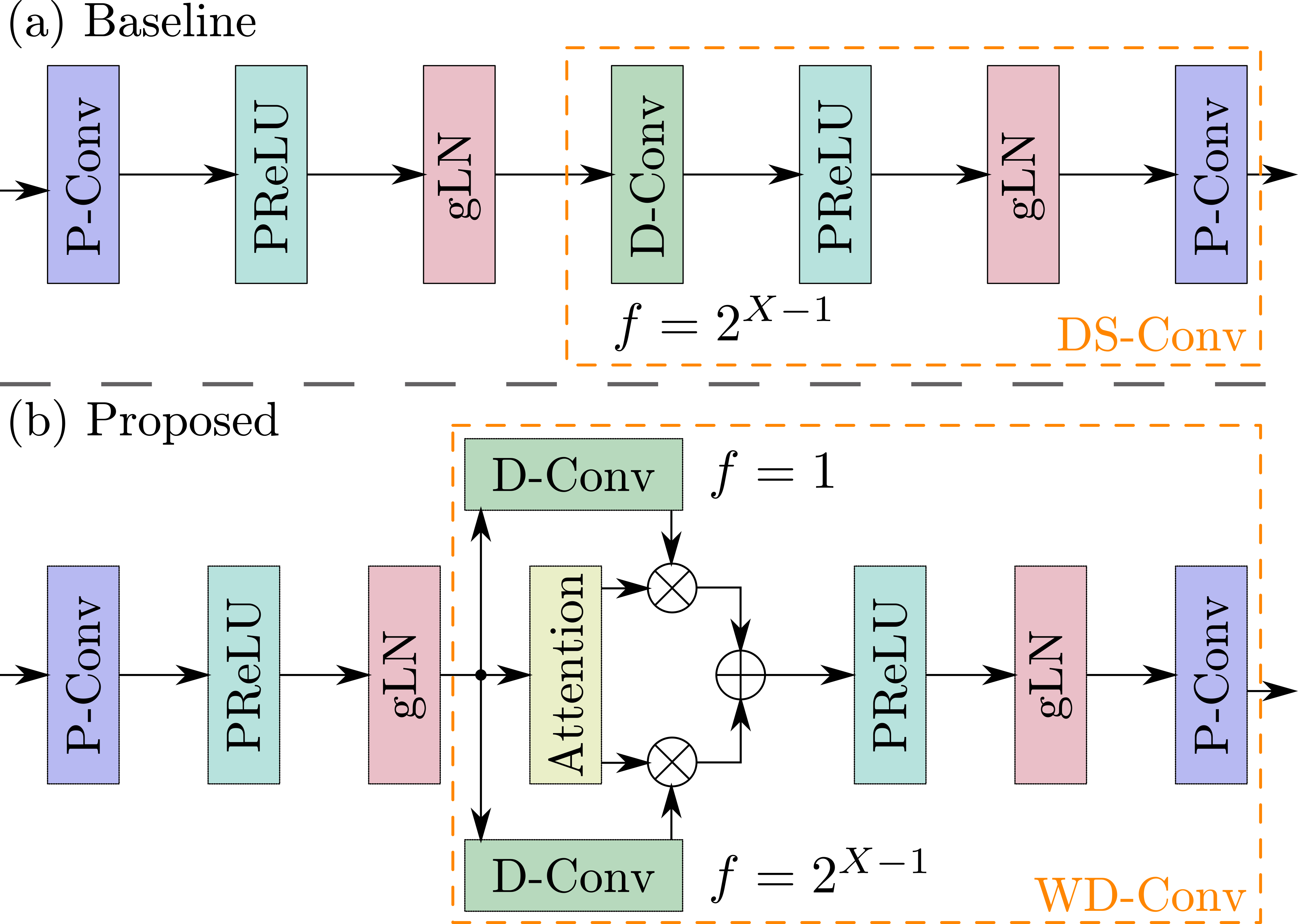
Fig. 1: (a) Convolutional block in baseline TCN; (b) Proposed convolutional block. Example for final block in a stack of conv. blocks for $Q=2$ with dilation factor $f=2^{X-1}$. Note that a residual connection around the entire block is omitted for brevity.

2.3.2 Weighted Multi-Dilation Depthwise-Separable Convolution (WD-Conv)

The WD-Conv network structure depicted in Fig. 1 (b) is proposed here as an extension to the DS-Conv operation where it is preferable to allow the network to be more selective about the temporal context to focus on without drastically increasing the number of parameters in the model. The proposed WD-Conv layer incorporates additional parallel D-Conv layers that can have a different dilation factor, hence it is referred to as dilation-augmented. The output of the D-Conv layers are weighted in a sum-to-one fashion and summed together. This summed output is then passed as the input to a P-Conv. In its simplest form the WD-Conv operation can be formulated as

$$\mathcal{W}\left(\mathbf{Y},\left(\mathbf{K}_{\mathcal{D}_{1},},\ldots,\mathbf{K}_{\mathcal{D}_{Q}}\right),\mathbf{K}_{\mathcal{P}}\right)=\\ \mathcal{P}\left(\sum_{q=1}^{Q}a_{q}\mathcal{D}_{q}\left(\mathbf{Y},\mathbf{K}_{\mathcal{D}_{q}}\right),\mathbf{K}_{\mathcal{P}}\right)$$ (8)

where $Q$ is the number of parallel D-Convs in the WD-Conv and $a_{q}$ are their corresponding weights that sum-to-one, i.e. $\sum_{q=1}^{Q}a_{q}=1$. In the model proposed here the number of D-Convs is set to $Q=2$ ; one with a dilation factor $f=1$ and the other according to the exponentially increasing dilation rule defined previously and used in [22, 19, 23] where $f$ is increasing in powers of 2 with every successive block in a stack of $X$ blocks. Note that the first convolutional blocks of a stack of $X$ blocks in the proposed implementation use an identical dilation of $f=1$ for each of the D-Conv kernels in the WD-Conv operation.

Inspired by the dynamic convolution kernel proposed in [21], the implementation proposed in this paper computes the weights for each D-Conv layer using an squeeze-and-excite (SE) attention network[26]. The SE attention network is shown in Fig. 2 and is composed of a global average pooling layer that reduces the sequence dimension from $L_{\mathbf{x}}$ to $1$ producing a vector of dimension $H$, the same as the feature dimension of the input. This feature vector is then compressed using a linear layer, with a rectified linear unit (ReLU) activation, to a dimension of $4$ as in [21]. The final stage is a linear layer that computes a weight for each of the D-Conv kernels in the WD-Conv structure. In the proposed model there are two D-Conv kernels and so the linear layer has an input dimension of $4$ and an output dimension of $2$. A softmax activation is used to ensure the sum-to-one constraint on the weights of the D-Conv layers.

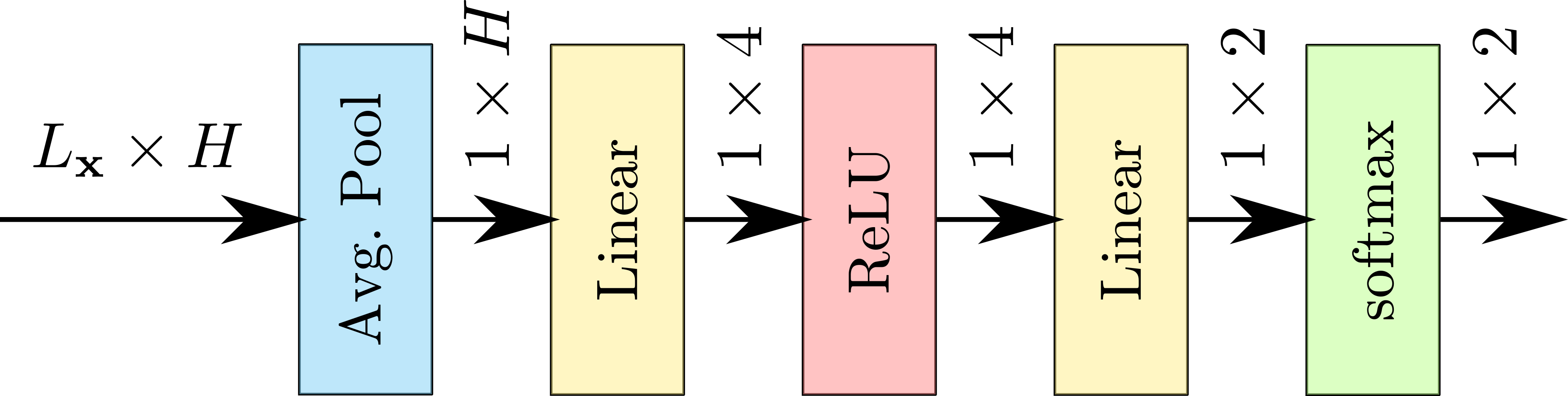
Fig. 2: Squeeze and excite attention weighting network. Output dimensionality of each layer is indicated above arrows.

2.4 Decoder

The decoder tansforms the encoded dereverberated signal $\mathbf{v}_{\ell}$ back into a time domain signal using a transposed 1D convolutional layer with $N$ input channels, $1$ output channel and a kernel size of $L_{\mathrm{BL}}$ such that

$$\hat{\mathbf{s}}_{\ell}=\mathbf{v}_{\ell}\mathbf{U}$$ (9)

where $\mathbf{U}\in\mathbb{R}^{N\times L_{\mathrm{BL}}}$ is a matrix of trainable convolutional weights and $\hat{\mathbf{s}}_{\ell}$ is an estimated dereverberated signal block in the time domain. The overlap-add method is used for re-synthesis of the signal from the overlapping blocks.

2.5 Objective Function

The objective function used here is the SISDR function [27] which is the same as that used to train the baseline TCN [19]. It is reformulated as a loss function by taking the negative SISDR value between the estimated speech segment $\hat{\mathbf{s}}$ and the reference direct path of the signal $\mathbf{s}_{\mathrm{dir}}$ defined as

$$\mathcal{L}_{\text{SISDR}}(\hat{\mathbf{s}},\mathbf{s}_{\mathrm{dir}}):=-10\log_{10}\frac{\left\|\frac{\langle\hat{\mathbf{s}},\mathbf{s}_{\mathrm{dir}}\rangle\mathbf{s}_{\mathrm{dir}}}{\|\mathbf{s}_{\mathrm{dir}}\|^{2}}\right\|^{2}}{\left\|\hat{\mathbf{s}}-\frac{\langle\hat{\mathbf{s}},\mathbf{s}_{\mathrm{dir}}\rangle\mathbf{s}_{\mathrm{dir}}}{\|\mathbf{s}_{\mathrm{dir}}\|^{2}}\right\|^{2}}.$$ (10)

3 Experimental Setup

3.1 Model and Training Configuration

Different model configurations are compared in the following to demonstrate the improvement gained by the proposed WD-TCN model across a range of model sizes. This is done by varying the number of convolutional blocks in a dilated stack $X$ as well as the number of times the dilated stack is repeated $R$. Based on previous work [19], the ranges of $X\in\{4,5,6,7,8\}$ and $R\in\{4,5,6,7,8\}$ were selected, resulting in 25 different configurations. All other parameters are fixed, i.e. kernel size $L_{\mathrm{BL}}=16$, number of encoder output channels $N=512$, number of bottleneck output channels $B=128$, number of channels inside the convolutional blocks $H=512$ and the kernel size inside each D-Conv $P=3$. For more details on these parameters see [19, 23, 22].

The same training approach as in [19] is used for both the baseline TCN and WD-TCN. Each model is trained for 100 epochs. An initial learning rate of $0.001$ is used and is halved if there is no improvement for 3 epochs. A batch size of 4 is used. The training was performed using the SpeechBrain speech processing toolkit [24]. The implementation of the proposed WD-TCN is available on GitHub.

3.2 Data

The simulated WHAMR noisy reverberant two speaker speech separation corpus [16] is used for the following experiments in this section. Only the reverberant and clean first speaker data is used for the input data $x[i]$ and target data $s_{\mathrm{dir}}[i]$. RIR are simulated using the pyroomacoustics software toolkit [28] and then convolved with the speech clips to produce the reverberant signal $x[i]$. The training set contains 20,000 samples for training which are truncated or padded to 4 s in length, to address sample length mismatches in batches and to also speed up training. There are 5000 samples (14.65 hrs) and 3000 samples (9 hrs) in the validation and test sets respectively.

3.3 Metrics

A number of metrics are used to assess a variety of properties in the dereverberated speech. The objective function SISDR is also used to measure distortions in signals. SRMR [29] is a measure used to directly measure reverberant effects in the signal. PESQ [30] and extended short-time objective intelligibility (ESTOI) [31] are objective measures used to assess the quality and intelligibility of signals.

4 Results

4.1 Performance Metrics and Model Size

The average SISDR results on the WHAMR evaluation set for the 25 chosen model configurations of the proposed WD-TCN model are given in Table 1 with SISDR improvements over the TCN model in the parenthesis. The bold font indicates best performance and highest improvement, respectively.

				$X$
		4	5	6	7	8
	4	11.21 (.28)	11.66 (.29)	11.81 (.40)	11.94 (.38)	12.04 (.40)
	5	11.51 (.41)	11.86 (.41)	11.94 (.23)	12.11 (.42)	12.11 (.39)
$R$	6	11.64 (.38)	11.95 (.30)	12.08 (.31)	12.09 (.23)	12.11 (.20)
	7	11.65 (.20)	12.17 (.44)	12.22 (.30)	12.16 (.13)	12.14 (.16)
	8	11.79 (.27)	12.03 (.19)	12.20 (.17)	12.21 (.22)	12.26 (.32)

Table 1: SISDR performance of WD-TCN with SE attention in dB. Numbers in $(\cdot)$ report performance improvement over baseline TCN.

These results show that the WD-TCN outperforms the TCN model across all 25 model configurations. The biggest performance gains are seen around $\{X,R\}=\{5,7\}$ and the WD-TCN model with most parameters and largest receptive field, $\{X,R\}=\{8,8\}$, shows best overall performance, contrary to the TCN model which gave the best SISDR results with $\{X,R\}=\{6,8\}$.

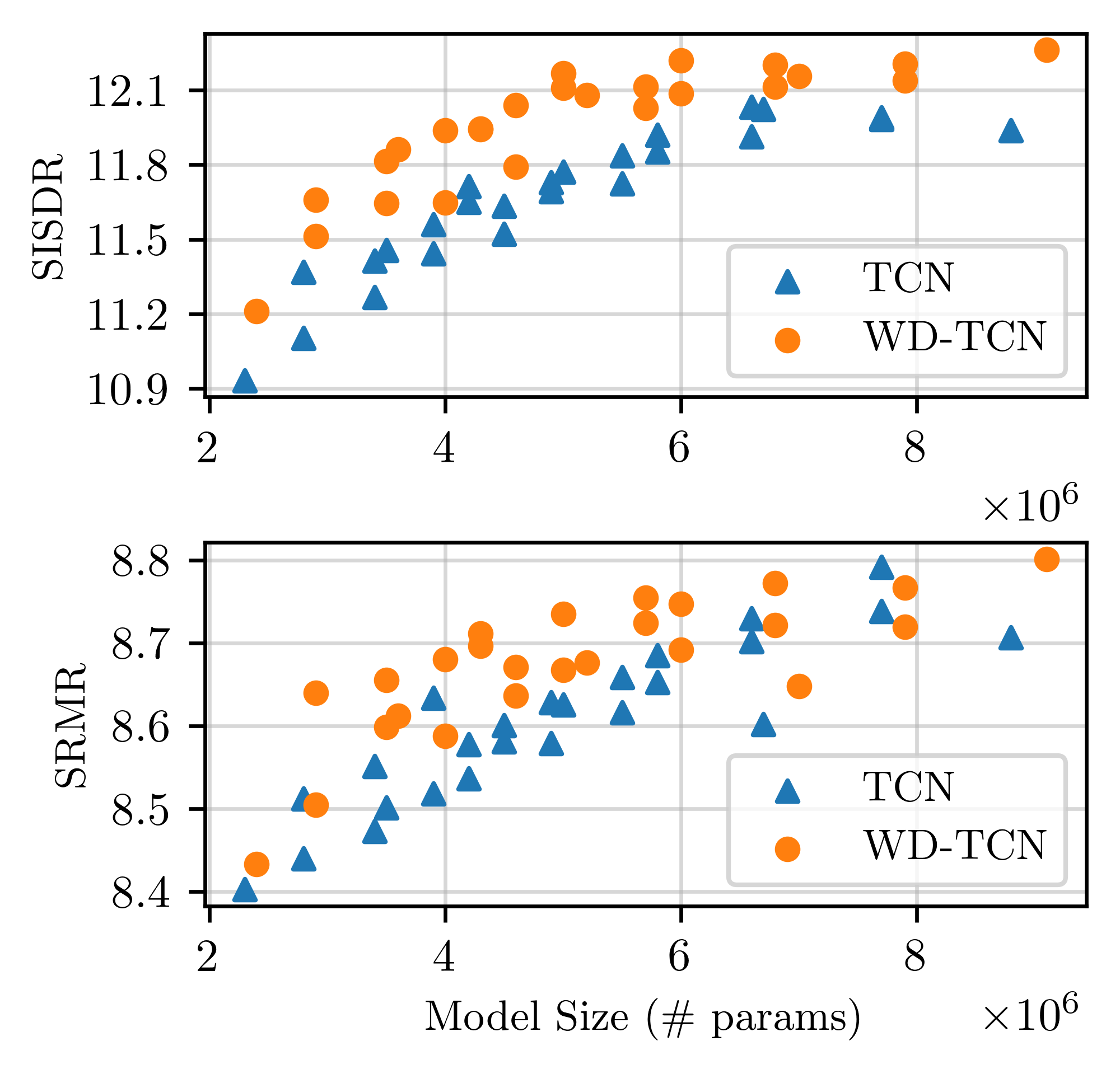
Fig. 3: Comparison of baseline TCN and WD-TCN over model size (no. of parameters) in terms of SISDR (top) and SRMR (bottom).

Fig. 3 (top) shows SISDR performance for all models over the model sizes in number of parameters. It can be seen that using the WD-TCN is a more parameter efficient approach to improving model performance than increasing the number of convolutional blocks (larger $X$ or $R$ values) in a conventional TCN. The SRMR performance against model size (Fig. 3, lower panel) shows the same findings, i.e. that the WD-TCN is a more parameter efficient approach to improving performance. For some larger models ($>$ 6M parameters) performance differs less. However the best performing model in terms of SRMR is still the WD-TCN.

Table 2 shows the results of the best performing TCN and WD-TCN models for each of the chosen performance metrics, highlighted in yellow, compared with the respective other model for the same $X$ and $R$ hyper-parameters. The performance in PESQ is inconclusive as many TCN models outperform their corresponding WD-TCN configurations but the best PESQ score of 3.5 is achieved with the WD-TCN model. The WD-TCN models show slightly better performance in ESTOI in line with the trend already observed in SRMR and SISDR. Note that SRMR is considered the most significant metric as it is designed to assess reverberation only.

Model	X	R	# params	SISDR	PESQ	ESTOI	SRMR
TCN	6	7	5.8M	11.92	3.46	0.930	8.65
WD-TCN	6	7	6.0M	12.22	3.5	0.933	8.69
TCN	6	8	6.6M	12.03	3.46	0.932	8.70
WD-TCN	6	8	6.8M	12.20	3.43	0.934	8.72
TCN	8	4	4.5M	11.63	3.48	0.927	8.60
WD-TCN	8	4	4.6M	12.04	3.45	0.931	8.67
TCN	8	7	7.7M	11.98	3.46	0.933	8.79
WD-TCN	8	7	7.9M	12.14	3.45	0.935	8.72
TCN	8	8	8.8M	11.94	3.46	0.933	8.71
WD-TCN	8	8	9.1M	12.26	3.45	0.935	8.8

Table 2: Best performing TCN and WD-TCN models compared corresponding models in SISDR, PESQ, ESTOI and SRMR. Bold indicates best performance per configuration, in terms of the $X$ and $R$ hyper-parameters. Results highlighted in yellow indicate best overall results for each model in each metric.

4.2 Squeeze-and-Excite Attention Analysis and T60 Variation

In the following, the attentive weights $a_{q}$ in (8) in the convolutional blocks are analysed. Note that $a_{1}$ corresponds to the attention weight applied to the D-Conv layers with the increasing dilation of $f\in\{1,2,\ldots,2^{X-1}\}$ for all convolutional blocks (cf. Fig. 1 (b)) and $a_{2}=$ is the weight corresponding to the D-Conv layers with the more local fixed dilation $f=1$. To analyse whether the SE attention approach was working as intended the attention weights were firstly computed across the entire evaluation set for every WD-TCN model trained in Table 1. Mean values of the weights for each model and each sample in the evaluation set were then computed and the evaluation set was in divided into increasing T60 ranges from 0.1s up to 1s. The mean for each weight $a_{q}$ over all models and samples, denoted as $\bar{a}_{q},q\in\{1,2\}$, was then computed for each T60 range. Figure 4 shows how the mean weight values vary across increasing T60 ranges. As the T60 range increases $\bar{a}_{1}$ increases. This demonstrates the SE attention approach is working as intended because the network has a less local focus within its receptive field for speech signals with larger reverberation times. Similarly the mean of the local attention weight $\bar{a}_{2}$ decreases as the T60 range increases demonstrating that the network is more focused on local information in its receptive field when the speech has a smaller reverberation time.

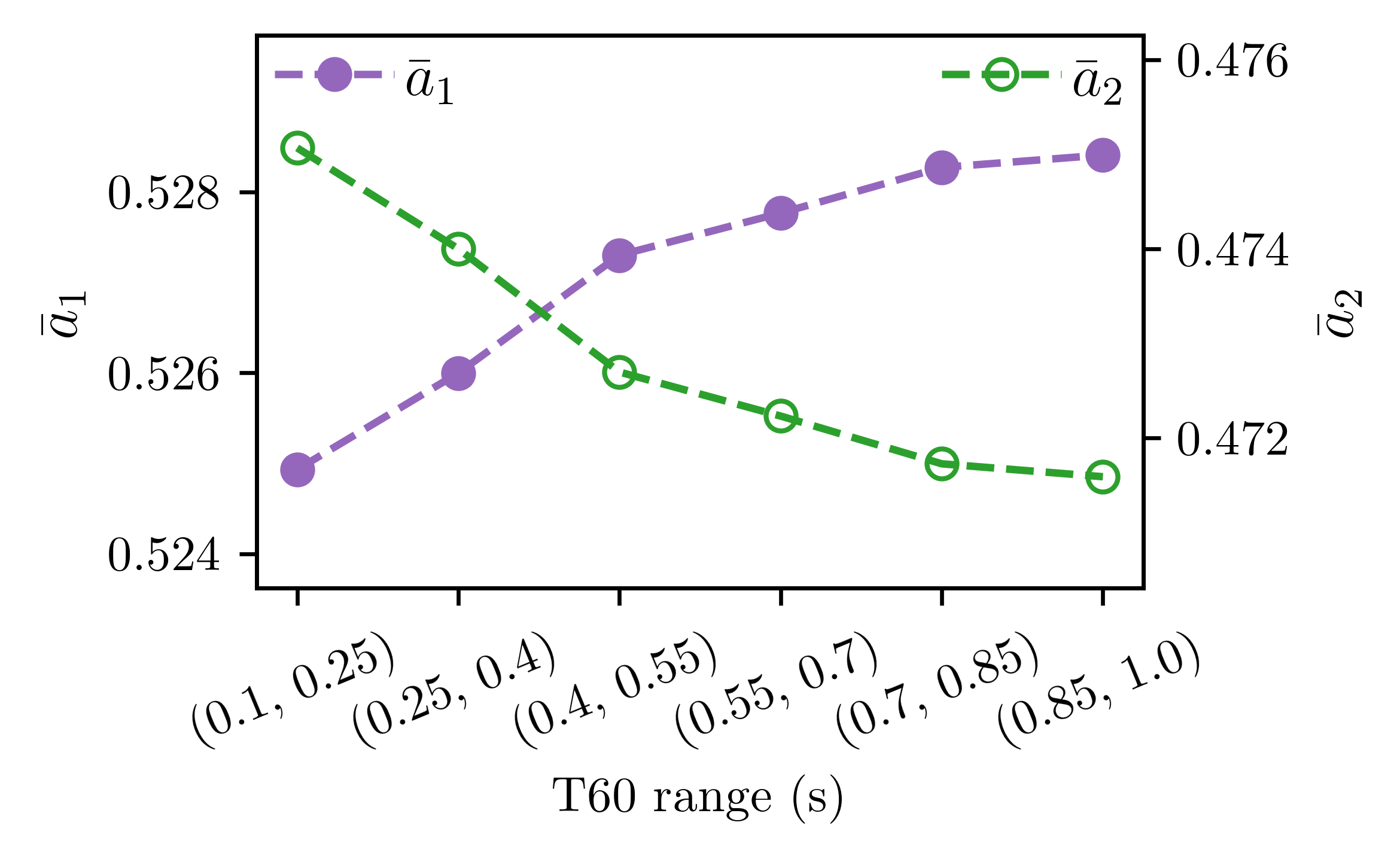
Fig. 4: Mean values of attention weights $\bar{a}_{q}$ across six different T60 ranges in the WHAMR evaluation set over all models with $X\in\{4,\ldots,8\}$ and $R\in\{4,\ldots,8\}$.

5 Conclusions

In this work, the WD-TCN model was proposed for TCN-based speech dereverberation by replacing depthwise-separable convolutions with weight multi-dilation depthwise-separable convolutions. It was shown that the WD-TCN consistently outperformed a conventional TCN across 25 different model configurations and that using the WD-TCN was a more parameter efficient approach to improving model performance than increasing the number of convolutional blocks in the TCN.

References

- [1] R. Haeb-Umbach, J. Heymann, L. Drude, S. Watanabe, M. Delcroix, and T. Nakatani, “Far-Field Automatic Speech Recognition,” Proceedings of the IEEE, vol. 109, no. 2, pp. 124–148, 2021.
- [2] F. Xiong, B.T. Meyer, N. Moritz, R. Rehr, J. Anemüller, T. Gerkmann, S. Doclo, and S. Goetze, “Front-end technologies for robust ASR in reverberant environments - spectral enhancement-based dereverberation and auditory modulation filterbank features,” EURASIP Journal on Advances in Signal Processing, vol. 2015, no. 1, 2015.
- [3] A. Purushothaman, A. Sreeram, R. Kumar, and S. Ganapathy, “Deep Learning Based Dereverberation of Temporal Envelopes for Robust Speech Recognition,” in Interspeech 2020, Oct. 2020.
- [4] R. Haeb-Umbach, S. Watanabe, T. Nakatani, M. Bacchiani, B. Hoffmeister, M. L. Seltzer, H. Zen, and M. Souden, “Speech processing for digital home assistants: Combining signal processing with deep-learning techniques,” IEEE Signal Processing Magazine, vol. 36, no. 6, pp. 111–124, 2019.
- [5] T. Hain, L. Burget, J. Dines, P. N. Garner, A. El Hannani, M. Huijbregts, M. Karafiát, M. Lincoln, and V. Wan, “The AMIDA 2009 meeting transcription system,” in Interspeech 2010, Sept. 2010.
- [6] G. Close, T. Hain, and S. Goetze, “MetricGAN+/-: Increasing Robustness of Noise Reduction on Unseen Data,” in EUSIPCO 2022, Aug. 2022.
- [7] E. A. P. Habets, Speech Dereverberation Using Statistical Reverberation Models, pp. 57–93, Springer London, London, 2010.
- [8] K. Kinoshita, M. Delcroix, H. Kwon, T. Mori, and T. Nakatani, “Neural Network-Based Spectrum Estimation for Online WPE Dereverberation,” in Interspeech 2017, Aug. 2017.
- [9] O. Ernst, S. E. Chazan, S. Gannot, and J. Goldberger, “Speech dereverberation using fully convolutional networks,” in EUSIPCO 2018, Sept. 2018.
- [10] Z. Wang and D. Wang, “Deep Learning Based Target Cancellation for Speech Dereverberation,” IEEE/ACM Transactions on Audio, Speech, and Language Processing, vol. 28, pp. 941–950, 2020.
- [11] H. Wang, B. Wu, L. Chen, M. Yu, J. Yu, Y. Xu, S. Zhang, C. Weng, D. Su, and D. Yu, “TeCANet: Temporal-Contextual Attention Network for Environment-Aware Speech Dereverberation,” in Interspeech 2021, Sept. 2021.
- [12] T. Zhao, Y. Zhao, S. Wang, and M. Han, “UNet++-Based Multi-Channel Speech Dereverberation and Distant Speech Recognition,” ISCSLP 2021, Jan. 2021.
- [13] Z. Wang, G. Wichern, and J. Le Roux, “Convolutive Prediction for Monaural Speech Dereverberation and Noisy-Reverberant Speaker Separation,” IEEE/ACM Transactions on Audio, Speech, and Language Processing, vol. 29, pp. 3476–3490, 2021.
- [14] Y. Fu, J. Wu, Y. Hu, M. Xing, and L. Xie, “DESNet: A Multi-Channel Network for Simultaneous Speech Dereverberation, Enhancement and Separation,” SLT 2021, Jan. 2021.
- [15] J. Su, Z. Jin, and A. Finkelstein, “HiFi-GAN: High-Fidelity Denoising and Dereverberation Based on Speech Deep Features in Adversarial Networks,” in Interspeech 2020, Oct. 2020.
- [16] M. Maciejewski, G. Wichern, and J. Le Roux, “WHAMR!: Noisy and reverberant single-channel speech separation,” in ICASSP 2020, May 2020.
- [17] Y. Zhao, D. Wang, B. Xu, and T. Zhang, “Monaural Speech Dereverberation Using Temporal Convolutional Networks With Self Attention,” IEEE/ACM Transactions on Audio, Speech, and Language Processing, vol. 28, pp. 1598–1607, 2020.
- [18] A. Pandey and D. Wang, “TCNN: Temporal Convolutional Neural Network for Real-time Speech Enhancement in the Time Domain,” in ICASSP 2019, May 2019.
- [19] W. Ravenscroft, S. Goetze, and T. Hain, “Receptive Field Analysis of Temporal Convolutional Networks for Monaural Speech Dereverberation,” in EUSIPCO 2022, Aug. 2022.
- [20] Y. Han, G. Huang, S. Song, L. Yang, H. Wang, and Y. Wang, “Dynamic neural networks: A survey,” IEEE Transactions on Pattern Analysis and Machine Intelligence, pp. 1–1, 2021.
- [21] Y. Chen, X. Dai, M. Liu, D. Chen, L Yuan, and Z. Liu, “Dynamic convolution: Attention over convolution kernels,” in CVPR 2020, June 2020.
- [22] Y. Luo and N. Mesgarani, “Conv-TasNet: Surpassing ideal time–frequency magnitude masking for speech separation,” IEEE/ACM Transactions on Audio, Speech, and Language Processing, vol. 27, no. 8, pp. 1256–1266, 2019.
- [23] W. Ravenscroft, S. Goetze, and T. Hain, “Att-TasNet: Attending to Encodings in Time-Domain Audio Speech Separation of Noisy, Reverberant Speech Mixtures,” Frontiers in Signal Processing, 2022.
- [24] M Ravanelli, T. Parcollet, P. Plantinga, A. Rouhe, S. Cornell, L. Lugosch, C. Subakan, N. Dawalatabad, A. Heba, J. Zhong, J. Chou, S. Yeh, S. Fu, C. Liao, E. Rastorgueva, F. Grondin, W. Aris, H. Na, Y. Gao, R. De Mori, and Y. Bengio, “SpeechBrain: A general-purpose speech toolkit,” 2021, arXiv:2106.04624.
- [25] K. He, X. Zhang, S. Ren, and J. Sun, “Delving deep into rectifiers: Surpassing human-level performance on imagenet classification,” in ICCV 2015, Dec. 2015.
- [26] J. Hu, L. Shen, and G. Sun, “Squeeze-and-excitation networks,” in CVPR 2018, June 2018.
- [27] J. Le Roux, S. Wisdom, H. Erdogan, and J. R. Hershey, “SDR – Half-baked or Well Done?,” in ICASSP 2019, May 2019.
- [28] R. Scheibler, E. Bezzam, and I. Dokmanić, “Pyroomacoustics: A python package for audio room simulation and array processing algorithms,” in ICASSP 2018, Apr. 2018.
- [29] J. F. Santos, M. Senoussaoui, and T. H. Falk, “An improved non-intrusive intelligibility metric for noisy and reverberant speech,” in IWAENC 2014, Sept. 2014.
- [30] A.W. Rix, J.G. Beerends, M.P. Hollier, and A.P. Hekstra, “Perceptual evaluation of speech quality (PESQ)-a new method for speech quality assessment of telephone networks and codecs,” in ICASSP 2001, May 2001.
- [31] J. Jensen and C. H. Taal, “An algorithm for predicting the intelligibility of speech masked by modulated noise maskers,” IEEE/ACM Transactions on Audio, Speech, and Language Processing, vol. 24, no. 11, pp. 2009–2022, 2016.