Dynamic Optimization Fabrics for Motion Generation

Abstract

Optimization fabrics are a geometric approach to real-time local motion generation, where motions are designed by the composition of several differential equations that exhibit a desired motion behavior. We generalize this framework to dynamic scenarios and non-holonomic robots and prove that fundamental properties can be conserved. We show that convergence to desired trajectories and avoidance of moving obstacles can be guaranteed using simple construction rules of the components. Additionally, we present the first quantitative comparisons between optimization fabrics and model predictive control and show that optimization fabrics can generate similar trajectories with better scalability, and thus, much higher replanning frequency (up to 500 Hz with a 7 degrees of freedom robotic arm). Finally, we present empirical results on several robots, including a non-holonomic mobile manipulator with 10 degrees of freedom and avoidance of a moving human, supporting the theoretical findings.

The open-source implementation can be found at https://github.com/tud-amr/fabrics

I Introduction

Robots increasingly populate dynamic environments. Imagine a robot operating alongside customers in a supermarket. It is requested to perform different tasks, such as cleaning the floor or picking a wide range of products. These different manipulation tasks may vary in their dimension and accuracy requirements, e.g. rotation around a suction gripper does not need to be specified while two-finger grippers require full poses. Thus, it is important for motion planning algorithms to support various goal definitions. Further, the robot is operating alongside humans, it has to constantly react to the changing environment and consequently update an initial plan. As customers move fast, the adaptations must be computed in real time. Therefore, motion planning is often divided into global motion planning [1] and local motion planning, which we will refer to as motion generation in this paper. A global planner generates a first feasible path that is used by a motion generator as global guidance. This paper proposes a novel approach to motion generation, that deals with a variety of different goal definitions.

Motion generation is often solved by formulating an optimization problem over a time horizon. The popularity of this approach is partly thanks to the guaranteed collision avoidance and thus safety [2, 3]. The optimization problem is then assembled from a scalar objective function, encoding the motion planning problem (e.g., the desired final position, path constraints, etc.), the transition function, defining the robot’s dynamics, and several inequality constraints, integrating physical limits and obstacle avoidance.

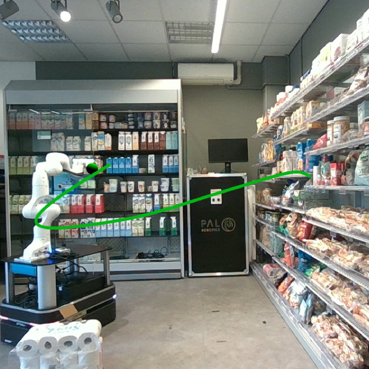
(a)

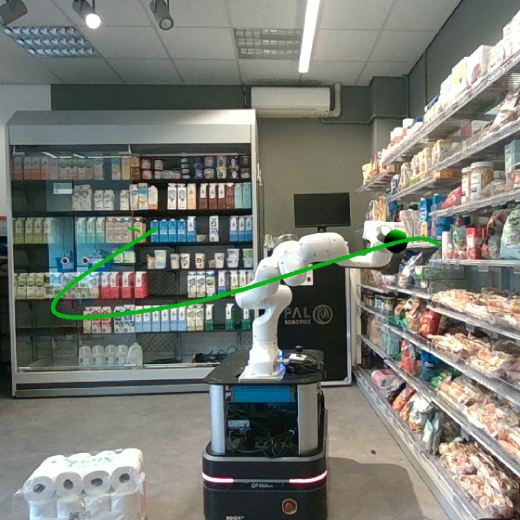
(b)

Figure 1: Dynamic fabrics for path (green) following with a non-holonomic mobile manipulator. Dynamic fabrics control all actuators simultaneously to follow the end-effector path while keeping a given orientation and avoiding collision with the environment.

Despite abundant applications of such optimization-based approaches to mobile robots, the computational costs limit applicability when dealing with high-dimensional configuration spaces [4, 5]. Data-driven approaches to speed up the optimization process usually come with reduced generalization abilities, loss of formal guarantees [3] and require prior, often costly, data acquisition. Moreover, due to the scalar objective function, the user must carefully weigh up different parts of the objective function. As a consequence, optimization-based approaches are challenging to tune and inflexible to generic motion planning problems with variable goal objectives [6, 7].

In the field of geometric control, namely Riemannian motion policies (RMP) and optimization fabrics, all individual parts of the motion planning problem are formulated as differential equations of second order. Applying operations from differential geometry, the individual components are combined in the configuration space to define the resulting motion [8, 9]. This allows to iteratively design the motion of the robot while maintaining explainability over the resulting motion [8, 9, 6, 10].

These works on optimization fabrics [9], but also on predecessors, such as RMP [8] and RMP-Flow [11], have shown the power of designing reactive behavior as second-order differential equations. However, integration of dynamic features, such as moving obstacles and path following, have not been proposed nor have the framework been applied to non-holonomic systems. In this article, we exploit relative coordinate systems in the framework of optimization fabrics by introducing the dynamic pullback operation (Eq. 8). This generalization can then integrate moving obstacles and path following. We show that our generalization maintains guaranteed convergence for path following tasks and improves collision avoidance with moving obstacles. Moreover, we propose a method to incorporate non-holonomic constraints. Lastly, we compare a trajectory optimization formulation, namely a model predictive control formulation, with optimization fabrics to provide the reader with a better understanding of key differences between the two approaches. We analyze computational costs and the quality of resulting trajectories for different robots. Several simulated results and real-world experiments show the practical implications of Dynamic Fabrics (DF). The contributions of this paper can be summarized as:

1. We enable the usage of optimization fabrics for dynamic scenarios. Specifically, we propose time parameterized differential maps using up-to second-order predictor models. As a consequence, this enables the integration of moving obstacles and path following tasks.

2. We extend the framework of optimization fabrics to non-holonomic robots.

3. We present a quantitative comparison between model predictive control and optimization fabrics. The results reveal that fabrics are an order of magnitude faster, more reliable, and easier to tune for goal-reaching tasks with a robotic manipulator in static environments.

All findings are supported by extensive experiments in both simulation and real-world with a manipulator, a differential drive robot, and a mobile manipulator.

II Related Work

In dynamic environments, global planning methods are not sufficient due to low planning frequencies. Thus, local motion generation methods, like the one presented in this work are employed. These methods typically require guidance to avoid local minima and thus effectively solve planning problems.

II-A Task constrained global motion planning

Motion planning problems are usually defined by goals in arbitrary task spaces, such as the 3D Euclidean space or end-effector poses. In this context, tasks can be regarded as constraints to the motion planning problem. Conventional approaches to motion planning rely on inverse kinematics to transform task constraints into sets of configurations. The resulting global motion planning problem is then often solved using sampling-based methods [12].

Sampling-based motion planners generate random configurations until a valid path between an initial configuration and a set of goal configurations is found [1]. Several methods have been proposed to directly integrate task constraints into the sampling phase. [13] proposed a method to iteratively push a random sample to the manifold adhering to the task constraint. The notion of task constraints was later extended to task space regions to define soft constraints for individual task components [14]. [15] proposed scalar-valued functions to represent task constraints for sampling-based planning. As all of the above-mentioned methods rely on implicitly constrained sampling in the joint space, they exhibit high computational time, which is especially harmful to real-world applications [16] and require local motion generation methods for path following and execution in dynamic environments [17]. In the next subsection, recent developments in local motion planning are summarized.

II-B Receding-horizon trajectory optimization

Methods formulating motion generation as an optimization problem with a finite discrete time horizon are known under the name of receding-horizon trajectory optimization. In line with most literature in robotics, we will refer to such methods as Model Predictive Control (MPC). Generally, several objectives are encoded in the scalar cost function, dynamics are formulated as equality constraints and inequality constraints ensure collision avoidance and joint limit avoidance. The dynamics for this problem can include the full dynamics model or simple integrating schemes [3]. By explicitly solving the constrained optimization problem, this approach yields formal guarantees on stability. Stability for MPC is proven by formulating an appropriate Lyapunov function and showing that the finite time-horizon formulation with an appropriate terminal cost results in the same stability as the corresponding infinite time-horizon formulation [18, 19, 20]. MPC has been applied to various robotic systems in dynamic environments, such as drones [21], mobile robots [17], and mobile manipulators [22, 23]. Despite these results, formal stability guarantees in such environments are challenging as appropriate terminal cost functions are often not computable or too conservative. Besides, the computational costs scale with the degrees of freedom restricting real-time applicability to simple dynamics and environment models [24].

Some MPC formulations are non-linear and can be analyzed using methods from non-linear control. When analyzing non-linear control system, Riemannian energies lead to more detailed stability results than Lyapunov functions. By investigating the variation around the generated trajectory and its contracting towards the desired trajectory, some control designs show exponential stabilizing properties [25]. These findings have been applied to tracking control problems [26].

II-C Riemannian motion policies and fabrics

Based on the findings of contracting metrics for non-linear control design [25, 26], geometric control approaches design the motion generation such that convergence is inherent to the problem formulation rather than imposing them on the solution process. Practically, individual constraints to the motion planning problem shape the optimization manifold so that the solution is accessible through the solution of simple differential equation. An example for shaping the optimization manifold is seen in Fig. 2.

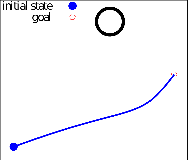
(a)

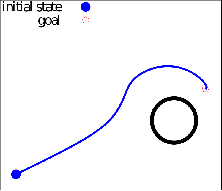
(b)

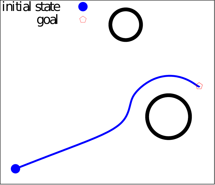
(c)

Figure 2: Combining different avoidance behaviors using optimization fabrics. The components defining collision avoidance with single obstacles (a,b) are combined in (c). Obstacles are shown in black. Trajectories of the point robot are shown in blue.

Realizing this concept, Riemannian motion policies (RMPs) represent a natural way of combining multiple policies into one joined policy. RMPs define individual sub-tasks of the motion planning as differential equations (spectral semi sprays or specs for short) of second order and propose the pullback and summation operators to combine multiple policies in the configuration space. As subtasks can be defined in arbitrary manifolds of the configuration space, RMP generalize operational space control [27]. The resulting behavior of RMP was reported to be intuitive while keeping computational costs low [28]. The concept of RMP was used in [8, 11] to form RMP-Flow, a motion planning algorithm that is shown to be conditionally stable and invariant across robots. In RMP-Flow, individual tasks are represented as a pair of a motion policy and a corresponding metric defining the importance of individual directions. An RMP adaptation was proposed for non-holonomic robots in [29]. By incorporating the kinematic constraint into the root equation of the RMP, the computed policy is applicable to non-holonomic robots. Besides, that work proposed a neural net to learn the collision avoidance task components.

Although RMPs have proven to be a powerful tool for motion generation, it was reported to require intuition and experience during tuning [9]. Optimization fabrics with Finsler structures as metric generators simplify the motion design as the conditions for stability and convergence are inherent to the definition of Finsler structures [9, 30]. Opposed to RMPs, where the metric is typically user-defined, fabrics derive Finsler metrics from artificial energies, similar to approaches from control design, [25, 26], using the Euler-Lagrange-Equation from geometric mechanics. Although fabrics generalize the concept of RMPs and make it accessible to a broader audience by decreasing the intuition and expertise required, they have not yet been applied to a wide range of robots.

The reason for this lack of application of fabrics is twofold. First, all the above mentioned methods are reactive and highly local methods, thus making them prone to local minima [31]. As RMPs and optimization fabrics do not incorporate path following, integration of global planning to overcome local minima is not possible to this date. Second, fabrics and RMP do not make use of velocity estimates of obstacles but rely purely on their high reactivity in dynamic environments. As for other trajectory optimization techniques, motion estimates could benefit fabrics (and RMP) to result in even smoother motion and allow applications in such environments.

In this paper, we address these issues by proposing time parameterized differential maps to form Dynamic Fabrics. This generalization integrates path following and velocity estimates of moving obstacles. Together with the extension to non-holonomic robots, our method allows to deploy the promising theory of optimization fabrics to mobile manipulators, operating in dynamic environments.

III Background

In the previous section, we have highlighted that optimization fabrics represent a powerful tool for reactive motion generation. Since we generalize this concept, this section aims at familiarizing the reader with key findings on optimization fabrics and recalling some of the basic notations known from differential geometry. We first give an overview on how optimization fabrics are used for motion generation and how the components are derived and composed. Then the theoretical foundations are summarized from [32, 9].

III-A Motion generation using optimization fabrics

When using optimization fabrics for motion generation, all components including constraints and goal attraction are designed as second order differential equations. If specific design rules for these equations are respected, all components can be combined to form a converging motion generator. Specifically, the following steps are performed:

1. Design path-consistent geometries in suited manifolds of the configuration space (Eq. 7).

2. Design corresponding Finsler energies defining the importance metric in this manifold (Section III-F).

3. Energize all geometries with the associated Finsler energies (Section III-F).

4. Pull back the energized systems into the configuration space and sum them (Section III-D).

5. Force the combined system with a differentiable potential. As a composition of optimization fabrics, the resulting trajectory converges towards the potential’s minimum (Section III-E).

In the following, we introduce the reader to the theory of optimization fabrics and recall important findings from [9].

III-B Configurations and task variables

We denote $\bm{q}\in\mathcal{Q}\subset\mathbb{R}^{n}$ a configuration of the robot with $n$ its degrees of freedom; $\mathcal{Q}$ is the configuration space of the generalized coordinates of the system. Generally, $\bm{q}(t)$ defines the robot’s configuration at time $t$, so that $\dot{\bm{q}}$, $\ddot{\bm{q}}$ define the instantaneous derivatives of the robot’s configuration. Similarly, we assume that there is a set of task variables $\bm{x}_{j}\in\mathcal{X}_{j}\subset\mathbb{R}^{m_{j}}$ with variable dimension $m_{j}\leq n$. The task manifold $\mathcal{X}_{j}$ defines an arbitrary manifold of the configuration space $\mathcal{Q}$ in which a robotic task can be represented. Further, we assume that there is a differential map $\phi_{j}:\mathbb{R}^{n}\rightarrow\mathbb{R}^{m_{j}}$ that relates the configuration space to the $j^{th}$ task space. For example, when a task variable is defined as the end-effector position, then $\phi_{j}$ is the positional part of the forward kinematics. On the other hand, if a task variable is defined to be the joint position, then $\phi_{j}$ is the identity function. In the following, we drop the subscript $j$ in most cases for readability when the context is clear.

In this work, we assume that $\phi$ is smooth and twice differentiable so that the Jacobian is defined as

$$\bm{J}_{\phi}=\frac{\partial\phi}{\partial\bm{q}}\in\mathcal{R}^{m\times n},$$ (1)

or $\bm{J}_{\phi}=\partial_{\bm{q}}\phi$ for short. Thus, we can write the total time derivatives of $\bm{x}$ as

$$\dot{\bm{x}} =\bm{J}_{\phi}\dot{\bm{q}}$$ (2)

$$\ddot{\bm{x}} =\bm{J}_{\phi}\ddot{\bm{q}}+\dot{\bm{J}}_{\phi}\dot{\bm{q}}.$$ (3)

III-C Spectral semi-sprays

Inspired by simple mechanics (e.g., the simple pendulum), the framework of optimization fabrics designs motion generation as second-order dynamical systems $\ddot{\bm{x}}=\pi(\bm{x},\dot{\bm{x}})$ [32, 9]. While higher-order systems seem feasible, their implementation on robots is much more challenging, as higher order configuration space derivatives would be required. The trajectory generator is defined by the differential equation $\bm{M}\ddot{\bm{x}}+\bm{f}=0$, where $\bm{M}(\bm{x},\dot{\bm{x}})$ and $\bm{f}(\bm{x},\dot{\bm{x}})$ are functions of position and velocity. Besides, $\bm{M}$ is symmetric and invertible. Such systems $\mathcal{S}=\left(\bm{M},\bm{f}\right)_{\mathcal{X}}$ are known as spectral semi-sprays, or specs for short. When the space of the task variable is clear from the context, we drop the subscript. Then, the trajectory is computed as the solution to the system $\ddot{\bm{x}}=-\bm{M}^{-1}\bm{f}$.

III-D Operations on specs

Next, the two fundamental operations for specs, transformation between spaces and summation, are introduced.

Given a differential map $\phi:\mathcal{Q}\rightarrow\mathcal{X}$ and a spec $\left(\bm{M},\bm{f}\right)_{\mathcal{X}}$, the pullback is defined as

$$\textrm{pull}_{\phi}{\left(\bm{M},\bm{f}\right)_{\mathcal{X}}}={\left(\bm{J}^{T}_{\phi}\bm{M}\bm{J}_{\phi},\bm{J}^{T}_{\phi}(\bm{f}+\bm{M}\dot{\bm{J}}_{\phi}\dot{\bm{q}})\right)}_{Q}.$$ (4)

The pullback allows converting between two distinct manifolds (e.g. a spec could be defined in the robot’s workspace and being pulled into the robot’s configuration space using the pullback with $\phi$ being the forward kinematics).

For two specs, $\mathcal{S}_{1}={\left(\bm{M}_{1},\bm{f}_{1}\right)}_{\mathcal{X}}$ and $\mathcal{S}_{2}={\left(\bm{M}_{2},\bm{f}_{2}\right)}_{\mathcal{X}}$, their summation is defined by:

$$\mathcal{S}_{1}+\mathcal{S}_{2}={\left(\bm{M}_{1}+\bm{M}_{2},\bm{f}_{1}+\bm{f}_{2}\right)}_{\mathcal{X}}.$$ (5)

III-E Optimization fabrics

Optimization fabrics form a special class of specs, and thus they inherit their properties, specifically the previously defined operations of summation and pullback. First, let us introduce a finite and differentiable potential function $\bm{\psi}(\bm{x})$ defined in a task manifold $\mathcal{X}$. Then, the modified spec $\mathcal{S}_{\bm{\psi}}=\left(\bm{M},\bm{f}+\partial_{\bm{x}}\bm{\psi}\right)$ is called the forced variant of $\mathcal{S}=\left(\bm{M},\bm{f}\right)_{\mathcal{X}}$. Only if the trajectory $\bm{x}(t)$ generated by the forced spec converges to the minimum of $\bm{\psi}$, the spec is said to form an optimization fabric. When the spec only converges to the minimum when equipped with a damping term, $\left(\bm{M},\bm{f}+\partial_{\bm{x}}\bm{\psi}+\bm{B}\dot{\bm{x}}\right)$, it forms a frictionless fabric [9, Definition 4.4]. Note that the mechanical system of a pendulum forms a frictionless fabric, as it optimizes the potential function defined by gravity when being damped (i.e., it eventually comes to rest at the configuration with minimal potential energy)

In the following, methods to construct optimization fabrics, or fabrics for short, are summarized: the definitions of conservative fabrics and energization are introduced.

III-F Conservative fabrics and energization

While the previous subsection defined what criteria are required for a spec to form an optimization fabric, the theory on conservative fabrics and energization offers a simple way of generating such special specs. As a full summary of the theory on optimization fabrics and their construction is out of scope here, this subsection only provides an outline of the theory and the reader is referred to [30, 10] for detailed derivations.

In the context of fabrics, the term energy describes a scalar quantity that changes as the system evolves over time. Although this quantity has a physical meaning in natural systems (e.g., kinetic energy), it can be arbitrarily defined for motion generation. Generally, specs and optimization fabrics do not conserve an energy, but when they do, we call them conservative specs. A stationary Lagrangian [9, Definition 4.11] is one definition for an energy for which the corresponding spec, known as the Lagrangian spec $\mathcal{S}_{\mathcal{L}_{e}}=\left(\bm{M}_{\mathcal{L}_{e}},\bm{f}_{\mathcal{L}_{e}}\right)$, is obtained by applying the Euler-Lagrange equations. Importantly, Lagrangian specs conserve energy and do thus belong to the class of conservative specs. It was proven that an unbiased ([9, Definition 4.11]) Lagrangian spec forms a frictionless fabric [9, Proposition 4.18]. Such fabrics are analogously called conservative fabrics. There are two classes of conservative fabrics: Lagrangian fabrics (i.e., the defining energy is a Lagrangian) and the more specific subclass of Finsler fabrics (i.e., the defining energy is a Finsler structure [9, Definition 5.4]).

The operation of energization transforms a given differential equation into a conservative spec. Specifically, given an unbiased energy Lagrangian $\mathcal{L}_{e}$ with boundary conforming $\bm{M}_{\mathcal{L}_{e}}$ [9, Definition 4.6] and lower bounded energy $\mathcal{H}_{e}$, an unbiased spec of form $\mathcal{S}_{\bm{h}}=(\bm{I},\bm{h})$ is transformed into a frictionless fabric using energization as

$$\begin{split}S_{\bm{h}}^{\mathcal{L}_{e}}&=\text{energize}_{\mathcal{L}_{e}}\{S_{\bm{h}}\}\\ &=(\bm{M}_{\mathcal{L}_{e}},\bm{f}_{\mathcal{L}_{e}}+\bm{P}_{\mathcal{L}_{e}}[\bm{M}_{\mathcal{L}_{e}}\bm{h}-\bm{f}_{\mathcal{L}_{e}}]),\end{split}$$ (6)

where $\bm{P}_{\mathcal{L}_{e}}=\bm{M}_{\mathcal{L}_{e}}\left(\bm{M}_{\mathcal{L}_{e}}^{-1}-\frac{\dot{\bm{x}}\dot{\bm{x}}^{T}}{\dot{\bm{x}}^{T}\bm{M}_{\mathcal{L}_{e}}\dot{\bm{x}}}\right)$ is an orthogonal projector. Energized specs maintain the energy of the Lagrangian and generally change the trajectory of the underlying spec $\mathcal{S}_{\bm{h}}$. However, if

1. $\mathcal{S}_{\bm{h}}=(\bm{I},\bm{h})$ is homogeneous of degree 2,

   $$\bm{h}(\bm{x},\alpha\dot{\bm{x}})=\alpha^{2}\bm{h}(\bm{x},\dot{\bm{x}})$$ (7)

   and

2. the energizing Lagrangian is a Finsler structure,

the resulting energized spec forms a frictionless fabric for which the trajectory matches the original trajectory of $\mathcal{S}_{\bm{h}}$. We refer to energized fabrics with that property as geometric fabrics. Geometric fabrics form the building blocks for motion generation with optimization fabrics. Practically, energization equips the individual components of the planning problem with a metric when being combined with other components.

III-G Experimental results fabrics

The theory explained above was tested on several simple kinematic chains in [9, 30]. As fabrics design motion as a summation of several differential equations, each representing a specific constraint to the motion, it is possible to sequentially design motion [9]. This procedure allows to carefully tune individual components without harming the others. The application to a planar arm in a goal-reaching setup was successfully tested in [9]. Here, the authors illustrated how the resulting motion can be modified arbitrarily by the user by adding additional constraints or preferences.

Although important concepts and findings on optimization fabrics were summarized in this section, we refer to [9] for a more in-depth presentation of optimization fabrics. In the following, we generalize the framework of optimization fabrics to dynamic settings.

IV Derivation of dynamic fabrics

We extend the framework of optimization fabrics to Dynamic Fabrics (DF). including dynamic environments and path following tasks. We prove that DF converge to moving goals and can be combined with previous approaches in geometric control. This section first introduces the notion of reference trajectory, dynamic Lagrangians and the dynamic pullback. These notations allow then to formulate DF. As DF generalize the concept of optimization fabrics to dynamic scenarios, we refer to the non-dynamic fabrics as Static Fabrics (SF) to explicitly distinguish between the work presented in [9] and our work.

IV-A Motion design using dynamic fabrics

The method explained in this paper generalizes the concept of SF from [9] and can then be extended from the procedure outlined in Section III-A.

1. Design path-consistent geometries in a suited, time-parameterized (Definition IV.2) manifold of the configuration

2. Design corresponding Finsler energies defining the importance metric in this manifold.

3. Energize all geometries with the associated Finsler energies.

4. If necessary, pull back the energized system from the time-parameterized manifold into the corresponding fixed manifold (Eq. 8).

5. Pull back the energized system into the configuration space and combine it with all components using summation.

6. Force the system with a time-parameterized potential. As a composition of DF, the resulting trajectory converges towards the potential’s minimum (Lemma IV.11).

In the following, we explain our proposed changes to the framework of SF so that it remains valid in dynamic environments.

IV-B Reference trajectories

To enable the definition of dynamic convergence and dynamic energy we introduce a reference trajectory that remains inside a domain $\mathcal{X}$ as boundary conforming. This term is chosen in accordance to [9, Definition 4.6].

Definition IV.1.

A reference trajectory $\bm{\tilde{x}}(t)$, with its corresponding time derivatives $\dot{\bm{\tilde{x}}}$ and $\ddot{\bm{\tilde{x}}}$, is boundary conforming on the manifold $\mathcal{X}$ if $\bm{\tilde{x}}(t)\in\mathcal{X},\forall t$.

In the following, the reference trajectory will be used to define dynamic Lagrangians and dynamic fabrics. In this context, the word ‘dynamic’ can often be read as ‘relative to the reference trajectory’. With the notion of reference trajectories we formulate a mapping to the relative coordinate system.

Definition IV.2.

Given a reference trajectory $\bm{\tilde{x}}$ on $\mathcal{X}$, the dynamic mapping $\phi_{d}:\mathcal{X}\times\mathcal{X}\to\mathcal{X}_{\textrm{rel}}$ represents the relative coordinate system $\bm{x}_{\textrm{rel}}=\bm{x}-\bm{\tilde{x}}$.

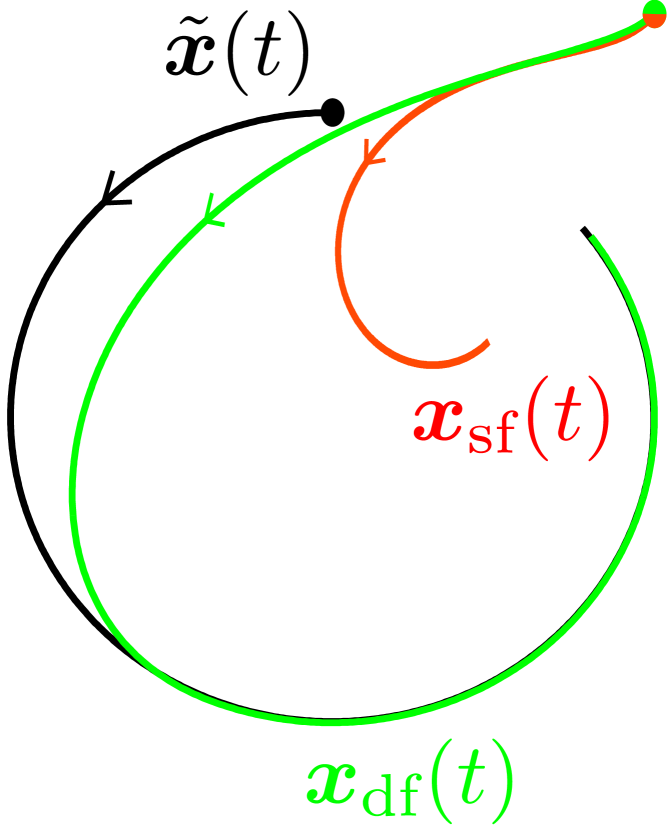
(a) Dynamic convergence

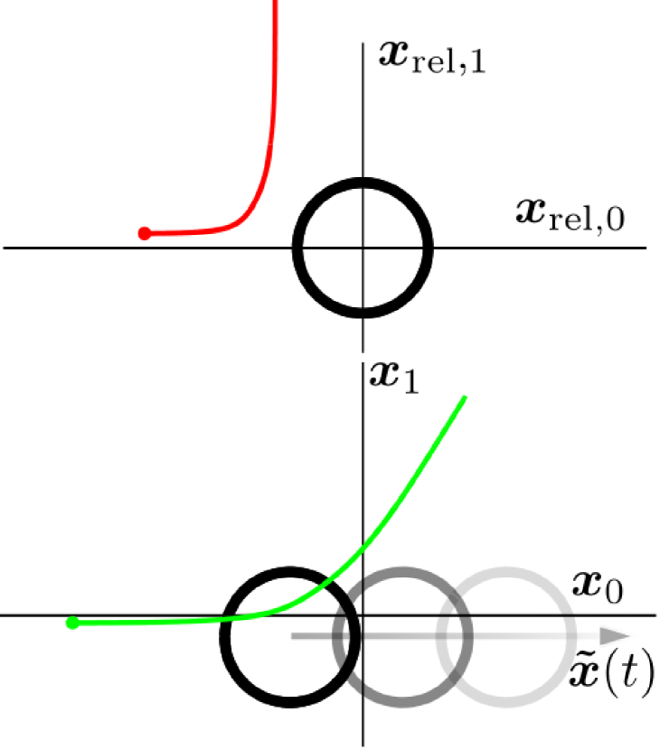
(b) Dynamic Avoidance

Figure 3: The two implications of Dynamic Fabrics. In (a), it can be seen that the trajectory obtained with DF (green) converges towards the reference trajectory (black) while the trajectory with Static Fabrics (red) does not converge. In (b), the top part visualizes collision avoidance as suggested in [9]. Here, the trajectory and obstacle are expressed in a relative system $\bm{x}_{\textrm{rel}}$. Using the dynamic pull, Eq. 8, this can be transformed into the static reference frame $\bm{x}$, bottom part. Together with dynamic energization, the framework of optimization fabrics is leveraged for dynamic environments. The motion of the obstacle, $\bm{x}_{\textrm{rel}}(t)$ is visualized with an arrow, future positions of the obstacle are shown in lighter color. The resulting trajectory obtained with DF is shown in green.

IV-C Dynamic pullback

The theory of optimization fabrics also applies to relative coordinates $\bm{x}_{\textrm{rel}}$, specifically, specs and potentials can be formulated in moving coordinates. However, there is no theory to combine specs defined in relative coordinates with specs in fixed coordinates. In most cases, individual components of the behavior design are not formulated in the same relative coordinates. Specificially, the configuration space is always static, so we introduce a transformation of a relative spec into the static space $\mathcal{X}$. We call this operation dynamic pullback.

$$\textrm{pull}_{\phi_{d}}{{(\bm{M}_{d},\bm{f}_{d})}_{\mathcal{X}_{\textrm{rel}}}}={(\bm{M}_{d},\bm{f}_{d}-\bm{M}_{d}\ddot{\bm{\tilde{x}}})}_{\mathcal{X}}$$ (8)

Two specs $\mathcal{S}_{\mathcal{X}_{\textrm{rel,1}}}$ and $\mathcal{S}_{\mathcal{X}_{\textrm{rel,2}}}$ defined in two different relative coordinate systems are then combined by first applying the dynamic pullback to both individually and then applying the summation operation for specs. The dynamic pullback is the natural extension to optimization fabrics for relative coordinate systems. It cannot directly be integrated into the framework of optimization fabrics as it breaks the algebra. In the following, we derive several generalizations so that the theory remains valid even in the presence of reference trajectories for individual components, such as moving obstacles or reference trajectories.

IV-D Dynamic Lagrangians

Next, we show that energy conservation commutes with the dynamic pullback. This allows us to transfer findings on conservative fabrics to dynamic fabrics. We call a Lagrangian that is defined using relative coordinates a dynamic Lagrangian and write $\mathcal{L}_{d}(\bm{x}_{\textrm{rel}},\dot{\bm{x}}_{\textrm{rel}})$. In this relative coordinate system, the dynamic Lagrangian has the same properties as the Lagrangian defined in [9], specifically it induces the Lagrangian spec through the Euler-Lagrange equation, $\partial^{2}_{\dot{\bm{x}}_{\textrm{rel}}\dot{\bm{x}}_{\textrm{rel}}}\mathcal{L}_{d}\ddot{\bm{x}}_{\textrm{rel}}+\partial^{2}_{\dot{\bm{x}}_{\textrm{rel}}\bm{x}_{\textrm{rel}}}\mathcal{L}_{d}\dot{\bm{x}}_{\textrm{rel}}-\partial_{\bm{x}_{\textrm{rel}}}\mathcal{L}_{d}$, as $(\bm{M}_{de},\bm{f}_{de})$. The system’s Hamiltonian $\mathcal{H}_{d}=\partial_{\dot{\bm{x}}_{\textrm{rel}}}\mathcal{L}_{d}^{T}\dot{\bm{x}}_{\textrm{rel}}-\mathcal{L}_{d}$ is conserved by the equation of motion as proven in [9].

Applying the dynamic pullback to the dynamic Lagrangian we obtain the transformed Lagrangian $\mathcal{L}_{d}(\bm{x},\dot{\bm{x}},\bm{\tilde{x}},\dot{\bm{x}})$ in the static coordinate system.

Theorem IV.3.

Let $\mathcal{L}_{d}(\bm{x}_{\textrm{rel}},\dot{\bm{x}}_{\textrm{rel}})$ be a dynamic Lagrangian and let $\phi_{d}$ be the dynamic mapping to $\bm{x}_{\textrm{rel}}$. Then, the application of the Euler-Lagrange equation commutes with the dynamic pullback.

Proof.

We will show the equivalence by calculation. As shown above, the induced spec is defined in the relative system as $(\bm{M}_{de},\bm{f}_{de})$. It can be dynamically pulled to form

$$\textrm{pull}_{\phi_{d}}{{(\bm{M}_{de},\bm{f}_{de})}_{\mathcal{X}_{\textrm{rel}}}}={(\bm{M}_{de},\bm{f}_{de}-\bm{M}_{de}\ddot{\bm{\tilde{x}}})}_{\mathcal{X}}$$ (9)

We can dynamically pull the Lagrangian $\mathcal{L}_{d}(\bm{x}_{\textrm{rel}},\dot{\bm{x}}_{\textrm{rel}})$ to form $\mathcal{L}_{d}(\bm{x},\dot{\bm{x}},\bm{\tilde{x}},\dot{\bm{\tilde{x}}})$, where only the first two variables are system variables. Using the generalized Euler-Lagrange equation, the equations of motion of the pulled Lagrangian are obtained as

$$0 =\frac{d}{dt}\frac{\partial\mathcal{L}_{d}}{\partial\dot{\bm{x}}}-\frac{\partial\mathcal{L}_{d}}{\partial\bm{x}}$$

$$=\frac{\partial^{2}\mathcal{L}_{d}}{\partial\dot{\bm{x}}\partial\dot{\bm{x}}}\ddot{\bm{x}}+\frac{\partial^{2}\mathcal{L}_{d}}{\partial\dot{\bm{x}}\partial\bm{x}}\dot{\bm{x}}+\frac{\partial^{2}\mathcal{L}_{d}}{\partial\dot{\bm{x}}\partial\dot{\bm{\tilde{x}}}}\ddot{\bm{\tilde{x}}}+\frac{\partial^{2}\mathcal{L}_{d}}{\partial\dot{\bm{x}}\partial\bm{\tilde{x}}}\dot{\bm{\tilde{x}}}-\frac{\partial\mathcal{L}_{d}}{\partial\bm{x}}$$

$$=\frac{\partial^{2}\mathcal{L}_{d}}{\partial\dot{\bm{x}}_{\textrm{rel}}\partial\dot{\bm{x}}_{\textrm{rel}}}\frac{\partial\dot{\bm{x}}_{\textrm{rel}}}{\partial\dot{\bm{x}}}\frac{\partial\dot{\bm{x}}_{\textrm{rel}}}{\partial\dot{\bm{x}}}\ddot{\bm{x}}+\frac{\partial^{2}\mathcal{L}_{d}}{\partial\dot{\bm{x}}_{\textrm{rel}}\partial\bm{x}_{\textrm{rel}}}\frac{\partial\dot{\bm{x}}_{\textrm{rel}}}{\partial\dot{\bm{x}}}\frac{\partial\bm{x}_{\textrm{rel}}}{\partial\bm{x}}\dot{\bm{x}}$$

$$+\frac{\partial^{2}\mathcal{L}_{d}}{\partial\dot{\bm{x}}_{\textrm{rel}}\partial\dot{\bm{x}}_{\textrm{rel}}}\frac{\partial\dot{\bm{x}}_{\textrm{rel}}}{\partial\dot{\bm{x}}}\frac{\partial\dot{\bm{x}}_{\textrm{rel}}}{\partial\dot{\bm{\tilde{x}}}}\ddot{\bm{\tilde{x}}}+\frac{\partial^{2}\mathcal{L}_{d}}{\partial\dot{\bm{x}}_{\textrm{rel}}\partial\bm{x}_{\textrm{rel}}}\frac{\partial\dot{\bm{x}}_{\textrm{rel}}}{\partial\dot{\bm{x}}}\frac{\partial\bm{x}_{\textrm{rel}}}{\partial\bm{\tilde{x}}}\dot{\bm{\tilde{x}}}$$

$$-\frac{\partial\mathcal{L}_{d}}{\partial\bm{x}_{\textrm{rel}}}\frac{\partial\bm{x}_{\textrm{rel}}}{\partial\bm{x}}$$

$$=\frac{\partial^{2}\mathcal{L}_{d}}{\partial\dot{\bm{x}}_{\textrm{rel}}\partial\dot{\bm{x}}_{\textrm{rel}}}\ddot{\bm{x}}+\frac{\partial^{2}\mathcal{L}_{d}}{\partial\dot{\bm{x}}_{\textrm{rel}}\partial\bm{x}_{\textrm{rel}}}\dot{\bm{x}}-\frac{\partial^{2}\mathcal{L}_{d}}{\partial\dot{\bm{x}}_{\textrm{rel}}\partial\dot{\bm{x}}_{\textrm{rel}}}\ddot{\bm{\tilde{x}}}$$

$$-\frac{\partial^{2}\mathcal{L}_{d}}{\partial\dot{\bm{x}}_{\textrm{rel}}\partial\bm{x}_{\textrm{rel}}}\dot{\bm{\tilde{x}}}-\frac{\partial\mathcal{L}_{d}}{\partial\bm{x}_{\textrm{rel}}}$$

$$=\frac{\partial^{2}\mathcal{L}_{d}}{\partial\dot{\bm{x}}_{\textrm{rel}}\partial\dot{\bm{x}}_{\textrm{rel}}}(\ddot{\bm{x}}-\ddot{\bm{\tilde{x}}})+\frac{\partial^{2}\mathcal{L}_{d}}{\partial\dot{\bm{x}}_{\textrm{rel}}\partial\bm{x}_{\textrm{rel}}}(\dot{\bm{x}}-\dot{\bm{\tilde{x}}})-\frac{\partial\mathcal{L}_{d}}{\partial\bm{x}_{\textrm{rel}}}$$

$$=\frac{\partial^{2}\mathcal{L}_{d}}{\partial\dot{\bm{x}}_{\textrm{rel}}\partial\dot{\bm{x}}_{\textrm{rel}}}(\ddot{\bm{x}}-\ddot{\bm{\tilde{x}}})+\frac{\partial^{2}\mathcal{L}_{d}}{\partial\dot{\bm{x}}_{\textrm{rel}}\partial\bm{x}_{\textrm{rel}}}(\dot{\bm{x}}_{\textrm{rel}})-\partial_{\bm{x}_{\textrm{rel}}}\mathcal{L}_{d}$$

$$=\bm{M}_{de}\ddot{\bm{x}}+\bm{f}_{de}-\bm{M}_{de}\ddot{\bm{\tilde{x}}}$$

The obtained equations of motion match the one obtained by applying the dynamic pullback, see Eq. 9. ∎

Hence, independently of the coordinates, the system conserves the energy $\mathcal{H}_{d}$ computed with the Hamiltonion in relative coordinates. Next, we adapt the operation of energization to dynamic Lagrangians. Dynamic Lagrangians are a necessary step to allow for collision avoidance with dynamic obstacles in the framework of optimization fabrics. Specifically, the metric for a moving obstacle is computed using the Euler-Lagrange equation in the relative coordinate system. Importantly, in this system, the same energies as with SF can be employed. Using the dynamic pullback, the energy defining the metric for the moving obstacle is then maintained according to Theorem IV.3. Concretely, this means that collision avoidance can be achieved in a similar manner as with SF with the added advantage of integrated motion estimates of obstacles.

Proposition IV.4 (Dynamic Energization).

Let ${\ddot{\bm{x}}+\bm{h}(\bm{x},\dot{\bm{x}})=\bm{0}}$ be a differential equation and suppose $\mathcal{L}_{d}$ is a dynamic Lagrangian with the induced spec $(\bm{M}_{de},\bm{f}_{de})$ and dynamic energy $\mathcal{H}_{d}$. Then the dynamically energized system $\ddot{\bm{x}}+\bm{h}(\bm{x},\dot{\bm{x}})+\alpha_{\mathcal{H}_{d}}\dot{\bm{x}}_{\textrm{rel}}=\bm{0}$ with

$$\alpha_{\mathcal{H}_{d}}=-{(\dot{\bm{x}}_{\textrm{rel}}^{T}\bm{M}_{de}\dot{\bm{x}}_{\textrm{rel}})}^{-1}\dot{\bm{x}}_{\textrm{rel}}^{T}(\bm{M}_{de}(\bm{h}+\ddot{\bm{\tilde{x}}})-\bm{f}_{de})$$

conserves the dynamic energy $\mathcal{H}_{d}$.

Proof.

From the derivations in [9], we can compute the rate of change of the dynamic energy as $\dot{\mathcal{H}_{d}}=\dot{\bm{x}}_{\textrm{rel}}^{T}(\bm{M}_{de}\ddot{\bm{x}}_{\textrm{rel}}+\bm{f}_{de})$. The equations of motion can be plugged in through the definition of the reference trajectory Definition IV.1, $\ddot{\bm{x}}_{\textrm{rel}}=\ddot{\bm{x}}-\ddot{\bm{\tilde{x}}}$ to obtain:

$$\dot{\mathcal{H}_{d}} =\dot{\bm{x}}_{\textrm{rel}}^{T}(\bm{M}_{de}(-\bm{h}-\alpha_{\mathcal{H}_{d}}\dot{\bm{x}}_{\textrm{rel}}-\ddot{\bm{\tilde{x}}})+\bm{f}_{de})$$

$$=\dot{\bm{x}}_{\textrm{rel}}^{T}(-\bm{M}_{de}\bm{h}-\bm{M}_{de}\dot{\bm{x}}_{\textrm{rel}}\alpha_{\mathcal{H}_{d}}-\bm{M}_{de}\ddot{\bm{\tilde{x}}}+\bm{f}_{de})$$

$$=\dot{\bm{x}}_{\textrm{rel}}^{T}(-\bm{M}_{de}\bm{h}$$

$$+\bm{M}_{de}\dot{\bm{x}}_{\textrm{rel}}{(\dot{\bm{x}}_{\textrm{rel}}^{T}\bm{M}_{de}\dot{\bm{x}}_{\textrm{rel}})}^{-1}\dot{\bm{x}}_{\textrm{rel}}^{T}(\bm{M}_{de}(\bm{h}+\ddot{\bm{\tilde{x}}})-\bm{f}_{de})$$

$$-\bm{M}_{de}\ddot{\bm{\tilde{x}}}+\bm{f}_{de})$$

$$=-\dot{\bm{x}}_{\textrm{rel}}^{T}\bm{M}_{de}\bm{h}+\dot{\bm{x}}_{\textrm{rel}}^{T}(\bm{M}_{de}(\bm{h}+\ddot{\bm{\tilde{x}}})-\bm{f}_{de})$$

$$-\dot{\bm{x}}_{\textrm{rel}}^{T}\bm{M}_{de}\ddot{\bm{\tilde{x}}}+\dot{\bm{x}}_{\textrm{rel}}^{T}\bm{f}_{de}$$

$$=0$$

The energized system conserves the dynamic energy. ∎

Proposition IV.4 allows to combine dynamic components of the motion generator with static components. Effectively, the dynamic component bends the underlying geometry according to the motion of the dynamic components (e.g., a moving obstacle).

While dynamic Lagrangians and the corresponding energization operation are similar to the methods described in [9], the operation of the standard pull to the dynamically energized system must be slightly modified. Specifically, the reference velocity must be pulled. We show that dynamic energization also commutes with the standard pullback.

Theorem IV.5.

Let $\mathcal{L}_{d}$ be a dynamic Lagrangian to the reference trajectory $\bm{\tilde{x}}$, and let $\ddot{\bm{x}}+\bm{h}(\bm{x},\dot{\bm{x}})=\bm{0}$ be a second order differential equation with a metric $\bm{M}_{d}$ such that $\bm{J}^{T}_{\phi}\bm{M}_{d}\bm{J}_{\phi}$ has full rank that can be written as spec $(\bm{M}_{d},\bm{M}_{d}\bm{h})$. Suppose $x=\phi(\bm{q})$ is a differential map with $\bm{J}_{\phi}$ its Jacobian. Then

$$\textrm{energize}_{\textrm{pull}_{\phi}{\mathcal{L}_{d}}}{\left(\textrm{pull}_{\phi}{(\bm{I},\bm{h})}\right)}=\textrm{pull}_{\phi}{\left(\textrm{energize}_{\mathcal{L}_{d}}{(\bm{I},\bm{h})}\right)},$$ (10)

when the reference velocity is being pulled as $\dot{\bm{\tilde{q}}}=\bm{J}_{\phi}^{\dagger}\dot{\bm{\tilde{x}}}$. $\bm{J}_{\phi}^{\dagger}$ denotes the pseudo-inverse of $\bm{J}_{\phi}$. We say that the dynamic energization operation commutes with the pullback transform.

Proof.

The commutation can be proven by calculation. First, we compute the right side of the equivalence. According to Proposition IV.4, the energized system (that maintains the dynamic energy $\mathcal{H}_{d}$) writes as

$$\bm{M}_{d}\ddot{\bm{x}}+\bm{M}_{d}\bm{h}+\alpha_{\mathcal{H}_{d}}(\dot{\bm{x}}-\dot{\bm{\tilde{x}}})=0,$$

with $\alpha_{\mathcal{H}_{d}}$ as defined in Proposition IV.4. Applying the pull-operation, we obtain

$$\bm{J}^{T}_{\phi}\bm{M}_{d}\bm{J}_{\phi}\ddot{\bm{q}}+\bm{J}^{T}_{\phi}\bm{M}_{d}\bm{h}+\bm{J}^{T}_{\phi}\bm{M}_{d}\dot{\bm{J}}_{\phi}\dot{\bm{q}}+\bm{J}^{T}_{\phi}\bm{M}_{d}\alpha_{\mathcal{H}_{d}}(\dot{\bm{x}}-\dot{\bm{\tilde{x}}})=0.$$ (11)

As the equation expressed in $\mathcal{X}$, this equation in $\mathcal{Q}$ maintains the energy $\mathcal{H}_{d}$. Next, we compute the left hand side. The equation of motion of the pulled dynamic Lagrangian $\mathcal{L}_{d}$ computes as

$$\textrm{pull}_{\phi}{(\bm{M}_{d},\bm{f}_{d})} =\bm{J}^{T}_{\phi}\left(\bm{M}_{d}\bm{J}_{\phi}\ddot{\bm{q}}+\bm{f}_{d}+\bm{M}_{d}\dot{\bm{J}}_{\phi}\dot{\bm{q}}-\bm{M}_{d}\ddot{\bm{\tilde{x}}}\right)$$

$$=\tilde{\bm{M}_{d}}\ddot{\bm{q}}+\tilde{\bm{f}_{d}}-\bm{J}^{T}_{\phi}\bm{M}_{d}\ddot{\bm{\tilde{x}}}.$$

The original spec is pulled accordingly

$$\textrm{pull}_{\phi}{(\bm{M}_{d},\bm{M}_{d}\bm{h})} =\bm{J}^{T}_{\phi}\bm{M}_{d}\bm{J}_{\phi}\ddot{\bm{q}}+\bm{J}^{T}_{\phi}\bm{M}_{d}\bm{h}+\bm{J}^{T}_{\phi}\bm{M}_{d}\dot{\bm{J}}_{\phi}\dot{\bm{q}}$$

$$=\tilde{\bm{M}_{d}}\ddot{\bm{q}}+\tilde{\bm{M}_{d}}\tilde{\bm{h}}$$

We energize the pulled system according to Proposition IV.4

$$\begin{split}\bm{J}^{T}_{\phi}\bm{M}_{d}\bm{J}_{\phi}\ddot{\bm{q}}+\bm{J}^{T}_{\phi}\bm{M}_{d}\bm{h}+\bm{J}^{T}_{\phi}\bm{M}_{d}\dot{\bm{J}}_{\phi}\dot{\bm{q}}\\ +\bm{J}^{T}_{\phi}\bm{M}_{d}\bm{J}_{\phi}\alpha_{\textrm{pull}_{\phi}{\mathcal{H}_{d}}}(\dot{\bm{q}}-\bm{J}_{\phi}^{\dagger}\dot{\bm{x}})=0,\end{split}$$ (12)

with

$$\alpha_{\textrm{pull}_{\phi}{\mathcal{H}_{d}}}= -{\left({(\dot{\bm{q}}-\bm{J}_{\phi}^{\dagger}\dot{\bm{\tilde{x}}})}^{T}\bm{J}^{T}_{\phi}\bm{M}_{d}\bm{J}_{\phi}(\dot{\bm{q}}-\bm{J}_{\phi}^{\dagger}\dot{\bm{\tilde{x}}})\right)}^{-1}$$

$${(\dot{\bm{q}}-\bm{J}_{\phi}^{\dagger}\dot{\bm{\tilde{x}}})}^{T}\left(\bm{J}^{T}_{\phi}\bm{M}_{d}\bm{J}_{\phi}(\tilde{\bm{h}}+\ddot{\bm{\tilde{x}}})\right.$$

$$-\left.\bm{J}^{T}_{\phi}\bm{f}_{d}-\bm{J}^{T}_{\phi}\bm{M}_{d}\dot{\bm{J}}_{\phi}\dot{\bm{q}}\right)$$

$$= -{\left({(\bm{J}_{\phi}\dot{\bm{q}}-\bm{J}_{\phi}\bm{J}_{\phi}^{\dagger}\dot{\bm{\tilde{x}}})}^{T}\bm{M}_{d}(\bm{J}_{\phi}\dot{\bm{q}}-\bm{J}_{\phi}\bm{J}_{\phi}^{\dagger}\dot{\bm{\tilde{x}}})\right)}^{-1}$$

$${(\dot{\bm{q}}-\bm{J}_{\phi}^{\dagger}\dot{\bm{\tilde{x}}})}^{T}\left(\bm{J}^{T}_{\phi}\bm{M}_{d}\bm{J}_{\phi}\tilde{\bm{h}}+\bm{J}^{T}_{\phi}\bm{M}_{d}\ddot{\bm{\tilde{x}}}\right.$$

$$\left.-\bm{J}^{T}_{\phi}\bm{f}_{d}-\bm{J}^{T}_{\phi}\bm{M}_{d}\dot{\bm{J}}_{\phi}\dot{\bm{q}}\right)$$

$$= -{\left({(\dot{\bm{x}}-\dot{\bm{\tilde{x}}})}^{T}\bm{M}_{d}(\dot{\bm{x}}-\dot{\bm{\tilde{x}}})\right)}^{-1}$$

$${(\dot{\bm{q}}-\bm{J}_{\phi}^{\dagger}\dot{\bm{\tilde{x}}})}^{T}\left(\bm{J}^{T}_{\phi}\bm{M}_{d}\bm{h}+\bm{J}^{T}_{\phi}\bm{M}_{d}\dot{\bm{J}}_{\phi}\dot{\bm{q}}+\bm{J}^{T}_{\phi}\bm{M}_{d}\ddot{\bm{\tilde{x}}}\right.$$

$$\left.-\bm{J}^{T}_{\phi}\bm{f}_{d}-\bm{J}^{T}_{\phi}\bm{M}_{d}\dot{\bm{J}}_{\phi}\dot{\bm{q}}\right)$$

$$= -{\left({(\dot{\bm{x}}-\dot{\bm{\tilde{x}}})}^{T}\bm{M}_{d}(\dot{\bm{x}}-\dot{\bm{\tilde{x}}})\right)}^{-1}$$

$${(\dot{\bm{q}}-\bm{J}_{\phi}^{\dagger}\dot{\bm{\tilde{x}}})}^{T}\left(\bm{J}^{T}_{\phi}\bm{M}_{d}\bm{h}+\bm{J}^{T}_{\phi}\bm{M}_{d}\ddot{\bm{\tilde{x}}}-\bm{J}^{T}_{\phi}\bm{f}_{d}\right)$$

$$= -{\left({(\dot{\bm{x}}-\dot{\bm{\tilde{x}}})}^{T}\bm{M}_{d}(\dot{\bm{x}}-\dot{\bm{\tilde{x}}})\right)}^{-1}$$

$${(\bm{J}_{\phi}\dot{\bm{q}}-\bm{J}_{\phi}\bm{J}_{\phi}^{\dagger}\dot{\bm{\tilde{x}}})}^{T}\left(\bm{M}_{d}\bm{h}+\bm{M}_{d}\ddot{\bm{\tilde{x}}}-\bm{f}_{d}\right)$$

$$= -{\left({(\dot{\bm{x}}-\dot{\bm{\tilde{x}}})}^{T}\bm{M}_{d}(\dot{\bm{x}}-\dot{\bm{\tilde{x}}})\right)}^{-1}{(\dot{\bm{x}}-\dot{\bm{\tilde{x}}})}^{T}$$

$$\left(\bm{M}_{d}\bm{h}+\bm{M}_{d}\ddot{\bm{\tilde{x}}}-\bm{f}_{d}\right)$$

$$=\alpha_{\mathcal{H}_{d}}$$

Thus, we have shown equivalence between $\alpha_{\mathcal{H}_{d}}$ and $\alpha_{\textrm{pull}_{\phi}{\mathcal{H}_{d}}}$. As $\alpha$ is scalar we can can rewrite the energization term in Eq. 12 as

$$\bm{J}^{T}_{\phi}\bm{M}_{d}\bm{J}_{\phi}\alpha_{\textrm{pull}_{\phi}{\mathcal{H}_{d}}}(\dot{\bm{q}}-\bm{J}_{\phi}^{\dagger}\dot{\bm{x}})$$

$$= \bm{J}^{T}_{\phi}\bm{M}_{d}\alpha_{\textrm{pull}_{\phi}{\mathcal{H}_{d}}}(\bm{J}_{\phi}\dot{\bm{q}}-\bm{J}_{\phi}\bm{J}_{\phi}^{\dagger}\dot{\bm{x}})$$

$$= \bm{J}^{T}_{\phi}\bm{M}_{d}\alpha_{\textrm{pull}_{\phi}{\mathcal{H}_{d}}}(\dot{\bm{x}}-\dot{\bm{x}})$$

$$= \bm{J}^{T}_{\phi}\bm{M}_{d}\alpha_{\mathcal{H}_{d}}(\dot{\bm{x}}-\dot{\bm{x}})$$

With the equivalence of the energization terms, we conclude the proof that dynamic energization commutes with the standard pullback. ∎

IV-E Dynamic fabrics

With the previous results, we formulate a new class of fabrics that converge to a reference trajectory. We call this class of fabrics Dynamic Fabrics. First, some notations are introduced to eventually show that dynamically energized specs form dynamic fabrics. Analogously to unbiased specs, we define dynamically unbiased specs (i.e., specs whose solutions do not diverge from the reference $\bm{\tilde{x}}$ when starting on the reference).

Definition IV.6.

A spec is said to be dynamically unbiased with respect to $\bm{\tilde{x}}(t)$ if $\bm{f}(\bm{x},\dot{\bm{x}})=-\bm{M}\ddot{\bm{\tilde{x}}}$, for $\bm{x}(t)=\bm{\tilde{x}}(t)$ and $\dot{\bm{x}}(t)=\dot{\bm{\tilde{x}}}(t)$.

Beside being dynamically unbiased, some specs will converge to the reference trajectory independently from their initial conditions.

Definition IV.7.

A spec is dynamically rough with respect to $\bm{\tilde{x}}(t)$ if all its integral curves $\bm{x}(t)$ converge dynamically with respect to $\bm{\tilde{x}}(t)$.

As for SF, DF can be formed by specs when they are being forced by a potential function $\bm{\psi}$. Such a forcing potential is generally a function of $\bm{x}$ and $\bm{\tilde{x}}$ and has at least one minimum. A spec that converges to a minimum of the forcing potential then forms a dynamic fabrics.

Definition IV.8.

A spec forms a dynamically rough fabric if it is dynamically rough with respect to $\bm{\tilde{x}}(t)$ when forced by a dynamic potential and $\exists t_{1}>0$ such that $\forall t>t_{1},\bm{x}(t)$ satisfies the Karush-Kuhn-Tucker (KKT) conditions for the optimization problem $\text{min}_{\bm{x}\in\mathcal{X}}\bm{\psi}(\bm{x},\bm{\tilde{x}}(t))$. If a spec does not form a dynamically rough fabric but all its damped variants do, it forms a dynamically frictionless fabric.

Theorem IV.9 (Dynamic Fabrics).

Suppose $S={(\bm{M},\bm{f})}_{\mathcal{X}}$ is a spec. Then $S$ forms a dynamically rough fabric with respect to $\bm{\tilde{x}}$ if and only if it is dynamically unbiased with respect to $\bm{\tilde{x}}$ and it converges dynamically when being forced by a dynamic potential $\bm{\psi}(\bm{x},\bm{\tilde{x}})$ with $\left\lVert\partial_{\bm{x}}\bm{\psi}\right\rVert<\infty$ on $\mathcal{X}$.

Proof.

We can write the corresponding differential equation

$$\bm{M}\ddot{\bm{x}}+\bm{f}=-\partial_{\bm{x}}\bm{\psi}$$ (13)

Assume that $S$ is dynamically unbiased. Since the spec converges with respect to $\bm{\tilde{x}}(t)$, we have $\dot{\bm{x}}\to\dot{\bm{\tilde{x}}},\bm{x}\to\bm{\tilde{x}}$. Because it is dynamically unbiased we also have $\bm{f}\to-\bm{M}\ddot{\bm{\tilde{x}}}$. Thus, the left hand side of Eq. 13, approaches $\bm{0}$. Consequently, the right hand side must also approach $\bm{0}$ and hence $\partial_{\bm{x}}\bm{\psi}\to\bm{0}$. The last satisfies the Karush–Kuhn–Tucker (KKT) conditions of $\bm{\psi}$.

To prove the converse, assume $\bm{f}$ dynamically biased. That implies that

$$\exists t>0,\bm{f}=\bm{M}\ddot{\bm{\tilde{x}}}+\bm{a}(\bm{\tilde{x}},\dot{\bm{\tilde{x}}}),\bm{a}(\bm{\tilde{x}},\dot{\bm{\tilde{x}}})\neq\bm{0}.$$

Hence, there exist a $t>0$ for which the left hand side does not vanish. As $\bm{\psi}$ satisifies the KKT conditions at $\bm{x}=\bm{\tilde{x}}$, its derivative equals zero at $\bm{x}=\bm{\tilde{x}}$ which contradicts Eq. 13 with $\bm{M}\bm{a}(\bm{\tilde{x}},\dot{\bm{\tilde{x}}})=\bm{0}$. ∎

Hence, the spec is required to be unbiased and convergent when forced. While the former can be verified using straight-forward computation, convergence is difficult to verify in the general case.

Lemma IV.10 (Dynamically energized fabrics).

Suppose $S$ is a dynamically unbiased energized spec. Then $S$ forms a dynamically frictionless fabric if $\partial_{\bm{x}}\bm{\psi}=-\partial_{\bm{\tilde{x}}}\bm{\psi}$.

Proof.

The equation of motion for the energized, forced and damped system writes as

$$\ddot{\bm{x}}+\bm{h}+\alpha_{\mathcal{H}_{d}}\dot{\bm{x}}_{\textrm{rel}}+\bm{B}\dot{\bm{x}}_{\textrm{rel}}+\partial_{\bm{x}}\bm{\psi}=0$$ (14)

The systems energy (dynamic Hamiltonian) is used as a Lyapunov function to show convergence. The rate of change is computed as

$$\dot{\mathcal{H}_{d}^{\bm{\psi}}} =\dot{\bm{x}}_{\textrm{rel}}^{T}(\bm{M}_{de}(-\bm{h}-\alpha_{\mathcal{H}_{d}}\dot{\bm{x}}_{\textrm{rel}}-\bm{B}\dot{\bm{x}}_{\textrm{rel}}-\partial_{\bm{x}}\bm{\psi}-\ddot{\bm{\tilde{x}}})$$

$$+\bm{f}_{de})+\dot{\bm{\psi}}$$

$$=-\dot{\bm{x}}_{\textrm{rel}}^{T}\bm{B}\dot{\bm{x}}_{\textrm{rel}}-\dot{\bm{x}}_{\textrm{rel}}^{T}\partial_{\bm{x}}\bm{\psi}+\dot{\bm{x}}^{T}\partial_{\bm{x}}\bm{\psi}+\dot{\bm{\tilde{x}}}^{T}\partial_{\bm{\tilde{x}}}\bm{\psi}$$

$$=-\dot{\bm{x}}_{\textrm{rel}}^{T}\bm{B}\dot{\bm{x}}_{\textrm{rel}}$$

As the system energy is lower bounded with $\mathcal{H}_{d}+\bm{\psi}\geq 0$ and $\dot{\mathcal{H}_{d}^{\bm{\psi}}}\leq 0$, when $\bm{B}$ stricly positive definite, we must have $\dot{\mathcal{H}_{d}^{\bm{\psi}}}\to 0$. Thus, $\dot{\bm{x}}_{\textrm{rel}}$ goes to zero. We can conclude that the system is dynamically converging. As it it also said to be dynamically unbiased, the damped energized system forms a dynamic fabric by Theorem IV.9. ∎

Lemma IV.11 (Dynamic Lagrangian fabrics).

An unbiased, dynamic Lagrangian spec forms a dynamically frictionless fabric if $\partial_{\bm{x}}\bm{\psi}=-\partial_{\bm{\tilde{x}}}\bm{\psi}$ holds for the forcing term.

Proof.

The equations of motion induced by the dynamic Lagrangian including damping and forcing are defined by the spec and can be written explicitly as

$$\bm{M}_{\mathcal{L}_{d}}\ddot{\bm{x}}_{\textrm{rel}}+\bm{f}_{\mathcal{L}_{d}}+\bm{B}\dot{\bm{x}}_{\textrm{rel}}+\partial_{\bm{x}}\bm{\psi}=0$$

$$\bm{M}_{\mathcal{L}_{d}}(\ddot{\bm{x}}-\ddot{\bm{\tilde{x}}})+\bm{f}_{\mathcal{L}_{d}}+\bm{B}(\dot{\bm{x}}-\dot{\bm{\tilde{x}}})+\partial_{\bm{x}}\bm{\psi}=0$$ (15)

$$\bm{M}_{\mathcal{L}_{d}}\ddot{\bm{x}}-\bm{M}_{\mathcal{L}_{d}}\ddot{\bm{\tilde{x}}}+\bm{f}_{\mathcal{L}_{d}}+\bm{B}\dot{\bm{x}}-\bm{B}\dot{\bm{\tilde{x}}}+\partial_{\bm{x}}\bm{\psi}=0$$

In the following we use the Hamiltonian and the potential function as Lyapunov function to show convergence of the damped spec.

$$\mathcal{H}_{d}^{\bm{\psi}}(\bm{x}) =\mathcal{H}_{d}+\bm{\psi}$$

$$=\partial_{\dot{\bm{x}}_{\textrm{rel}}}\mathcal{L}_{d}^{T}\dot{\bm{x}}_{\textrm{rel}}-\mathcal{L}_{d}+\bm{\psi}$$

The time derivative is composed of the time derivative of the Hamiltonian, $\dot{\mathcal{H}_{e}}=\dot{\bm{x}}_{\textrm{rel}}^{T}(\bm{M}_{\mathcal{L}_{d}}\ddot{\bm{x}}_{\textrm{rel}}+\bm{f}_{\mathcal{L}_{d}})$, and the time derivative of the forcing potential, $\dot{\bm{\psi}}=\dot{\bm{x}}^{T}\partial_{\bm{x}}\bm{\psi}+\dot{\bm{\tilde{x}}}^{T}\partial_{\bm{\tilde{x}}}\bm{\psi}$. Thus, the system’s total energy varies over time:

$$\dot{\mathcal{H}_{d}}^{\bm{\psi}}(\bm{x})={(\dot{\bm{x}}-\dot{\bm{\tilde{x}}})}^{T}(\bm{M}_{\mathcal{L}_{d}}(\ddot{\bm{x}}-\ddot{\bm{\tilde{x}}})+\bm{f}_{\mathcal{L}_{d}})+\dot{\bm{x}}^{T}\partial_{\bm{x}}\bm{\psi}+\dot{\bm{\tilde{x}}}^{T}\partial_{\bm{\tilde{x}}}\bm{\psi}$$

Plugging in the equations of motion Eq. 15 gives

$$\dot{\mathcal{H}_{d}}^{\bm{\psi}}(\bm{x}) ={(\dot{\bm{x}}-\dot{\bm{\tilde{x}}})}^{T}(-\bm{f}_{\mathcal{L}_{d}}-\bm{B}(\dot{\bm{x}}-\dot{\bm{\tilde{x}}})-\partial_{\bm{x}}\bm{\psi}+\bm{f}_{\mathcal{L}_{d}})$$

$$+\dot{\bm{x}}^{T}\partial_{\bm{x}}\bm{\psi}+\dot{\bm{\tilde{x}}}^{T}\partial_{\bm{\tilde{x}}}\bm{\psi}$$

$$=-{(\dot{\bm{x}}-\dot{\bm{\tilde{x}}})}^{T}\bm{B}(\dot{\bm{x}}-\dot{\bm{\tilde{x}}})-{(\dot{\bm{x}}-\dot{\bm{\tilde{x}}})}^{T}\partial_{\bm{x}}\bm{\psi}$$

$$+\dot{\bm{x}}^{T}\partial_{\bm{x}}\bm{\psi}+\dot{\bm{\tilde{x}}}^{T}\partial_{\bm{\tilde{x}}}\bm{\psi}$$

$$=-{(\dot{\bm{x}}-\dot{\bm{\tilde{x}}})}^{T}\bm{B}(\dot{\bm{x}}-\dot{\bm{\tilde{x}}})+\dot{\bm{\tilde{x}}}^{T}(\partial_{\bm{x}}\bm{\psi}+\partial_{\bm{\tilde{x}}}\bm{\psi}).$$

For $\partial_{\bm{x}}\bm{\psi}=-\partial_{\bm{\tilde{x}}}\bm{\psi}$ and $\bm{B}$ strictly positive definite, $\dot{\mathcal{H}_{d}}$ is strictly negative for $(\dot{\bm{x}}-\dot{\bm{\tilde{x}}})\neq 0$. Since $\mathcal{H}_{d}^{\bm{\psi}}$ is lower bounded as composition of lower bounded function and $\dot{\mathcal{H}_{d}}^{\bm{\psi}}\leq 0$, $\dot{\mathcal{H}_{d}}^{\bm{\psi}}\to 0$ and thus, $\dot{\bm{x}}\to\dot{\bm{\tilde{x}}}$ and $\bm{x}\to\bm{\tilde{x}}$. Hence, the spec converges dynamically with respect to $\bm{\tilde{x}}$. As the spec is further said to be dynamically unbiased, the damped spec forms a dynamic fabric by Theorem IV.9. ∎

Concretely, Lemma IV.11 allows for trajectory following with guaranteed convergence with DF. For example, a reference trajectory for the robot’s end-effector is defined as $\bm{\tilde{x}}(t)$. Then, the potential can be designed as $\psi=\bm{\tilde{x}}(t)-\bm{x}$ (respecting the construction rule required for Lemma IV.11). In contrast to SF, where the static potential function is simply updated at every time step, DF makes use of the dynamics of the reference trajectory through the dynamic pullback.

IV-F Construction procedure

From the high-level procedure explained in Section IV-A, we can derive the algorithm using the formal findings in this section, see Algorithm 1.

Define basic inertia as spec $\bm{M}\ddot{\bm{q}}+\bm{M}\bm{h}=0$

for avoidance in avoidances do

       Define differential map between $\mathcal{Q}$ and $\mathcal{X}_{i}$: $\phi$ or $\phi_{t}$

       Design geometry on $\mathcal{X}_{i}$: $\ddot{\bm{x}}_{i}+\bm{h}_{2,i}=\bm{0}$

       Design Finsler energy for behavior on $\mathcal{X}_{i}$: $\mathcal{L}_{i}$

       Energize geometry with Finsler energy IV.4

       if $\phi$ is time-parameterized then

             Apply dynamic pullback to energized system

            

       end if

      Apply standard pullback

       Add pulled avoidance component to root fabric

      

end for

Force root system with (time-parameterized) potential

Algorithm 1 Motion design with dynamic fabrics

Methods to design the individual components, such as geometry and Finsler structures, are introduced in [9]. As these design patterns do not vary for DF, they are not repeated here. In the result section, we show some experimental examples highlighting the comparative advantage of optimization fabrics over model predictive schemes and the advantage of DF over SF for dynamic environments.

V Extension to non-Holonomic Constraints

Mobile manipulators are often equipped with a non-holonomic base (e.g., a differential drive mobile robot). In contrast to revolute joints for manipulators, non-holonomic bases imply non-holonomic constraints. Based on ideas presented in [29], we propose a method to integrate such constraints in optimization fabrics, including DF.

We assume that the non-holonomic constraint at hand can be expressed as an equality of form

$$\dot{\bm{x}}=\bm{J}_{\textrm{nh}}\dot{\bm{q}},$$ (16)

where $\bm{J}_{\textrm{nh}}$ is the Jacobian of the constraint, $\dot{\bm{q}}$ is the velocity of the controlled joints of the system and $\dot{\bm{x}}$ is the root velocity of the fabric. For a differential drive $\dot{\bm{x}}$ is the velocity of the system in the Cartesian plane ($\dot{x},\dot{y},\dot{\theta}$) and $\dot{\bm{q}}$ is the velocity of the actuated wheels ($u_{\textrm{left}},u_{\textrm{right}}$). Moreover, we assume that Eq. 16 is smooth and differentiable so that we can write

$$\ddot{\bm{x}}=\dot{\bm{J}}_{\textrm{nh}}\dot{\bm{q}}+\bm{J}_{\textrm{nh}}\ddot{\bm{q}}.$$ (17)

The theory of optimization fabrics allows to pull a tree of fabrics back into one fabric expressed in its root-coordinates of form $\bm{M}\ddot{\bm{x}}+\bm{f}=0$ with its solution as

$$\ddot{\bm{x}}=-\bm{M}^{-1}\bm{f}.$$ (18)

Plugging Eq. 17 into the root fabric we obtain the non-holonomic fabric of form

$$\bm{M}\bm{J}_{\textrm{nh}}\ddot{\bm{q}}+\bm{M}\dot{\bm{J}}_{\textrm{nh}}\dot{\bm{q}}+\bm{f} =0$$

$$\bm{M}_{\textrm{nh}}\ddot{\bm{q}}+\bm{f}_{\textrm{nh}} =0$$

.

Note that $\bm{M}_{\textrm{nh}}$ is not necessarily a square matrix and thus not invertible as it was in the original fabric. To find the best actuation for the wheels, we formulate motion generation with fabrics as an unconstrained optimization problem

$$\ddot{\bm{q}}^{\ast}=\min_{\ddot{\bm{q}}}\left\lVert\bm{M}_{\textrm{nh}}\ddot{\bm{q}}+\bm{f}_{\textrm{nh}}\right\rVert_{2}^{2}.$$ (19)

In this approach, we minimize the error of the final equation. We could equally derive Eq. 19 with the objective of minimizing the error between $\ddot{\bm{x}}=\bm{J}_{\textrm{nh}}\ddot{\bm{q}}+\dot{\bm{J}}_{\textrm{nh}}\dot{\bm{q}}$ and the original fabric’s solution $\ddot{\bm{x}}=-\bm{M}\bm{f}$. The mimization of the difference leads to similar result. This optimization problem replaces Eq. 18 and is solved by

$$\ddot{\bm{q}}^{\ast}=\bm{M}_{\textrm{nh}}^{\dagger}\bm{f}_{\textrm{nh}}.$$ (20)

The solutions to this problem makes optimization fabrics, and thus dynamic fabrics, applicable to non-holonomic robots, such as differential drive robots or cars. A qualitative comparison between a trajectory generated for a holonomic and a non-holonomic robot is shown in Fig. 4.

(a) 7s

(b) 11s

(c) 18s

(d) 7s

(e) 11s

(f) 18s

Figure 4: Path (green) following with a holonomic and a non-holonomic robot using DF with the extension to non-holonomic robots

The theory of optimization fabrics is built upon energy conservation of artificial energies that design the motion. Eq. 19 does not solve the resulting spec exactly, but minimizes the deviation according to the least square objective function. For many kinematic systems, e.g., differential drive model, bicycle model, the non-holonomic constraint additionally reduces the number of degrees of freedom, $\dim{q}<\dim{x}$. As a consequence, the least square solution has a non-zero residuum. Then, some fundamental properties of optimization fabrics, such as energy conservation and convergence can no longer be guaranteed. Despite this theoretical shortcoming, we show that this approach leads to good performance in practical applications.

VI Experimental results

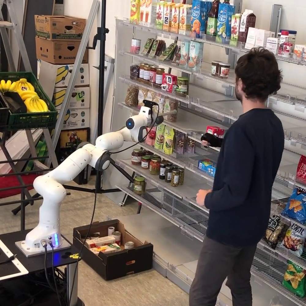
(a) $t=0$s

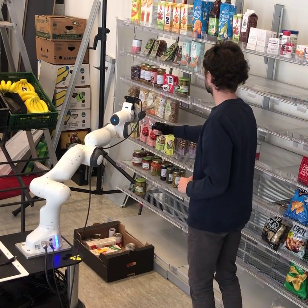
(b) $t=2$s

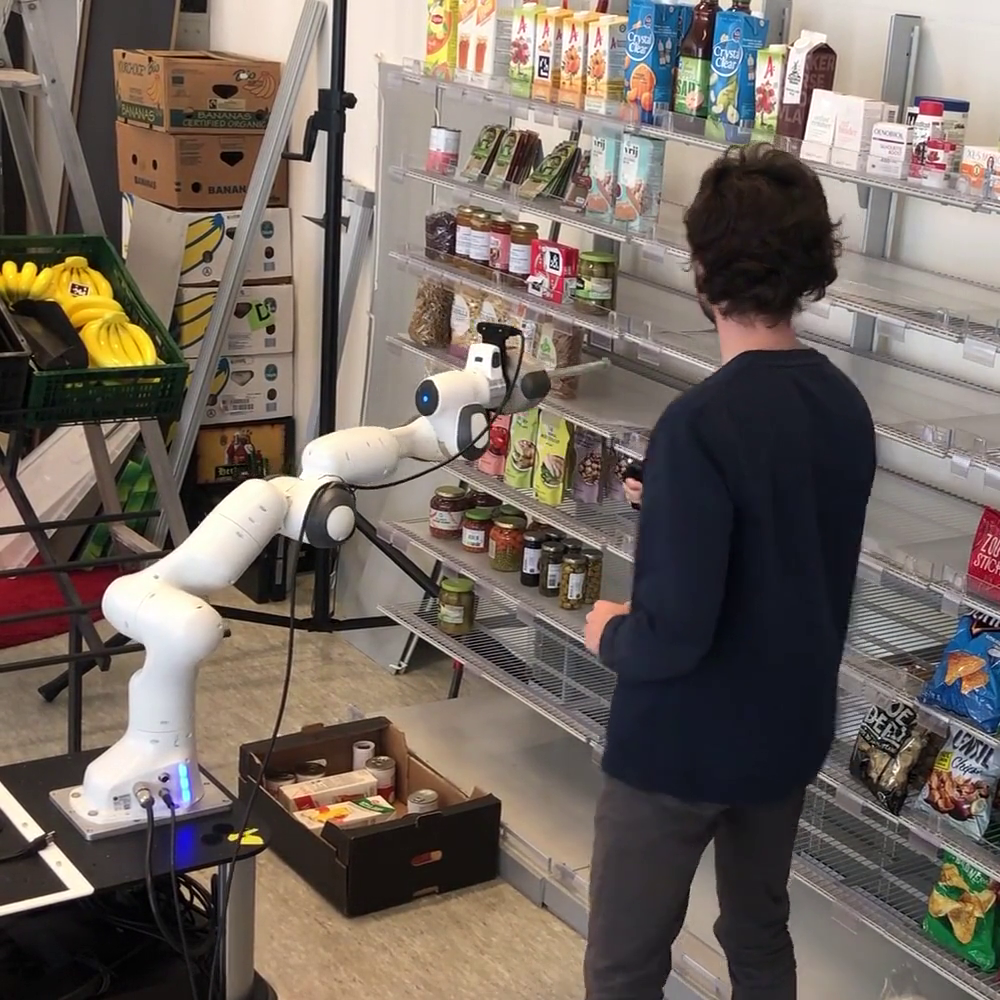
(c) $t=3$s

Figure 5: Dynamic Fabrics in the presence of a human. The human hand’s state is estimated with a motion capture system. The robot smoothly and in advance avoids the human operator and allows for safe coexistence.

In this section, the performance of optimization fabrics is assessed on various robotic platforms. Although [9] suggested performance benefits over optimization-based methods to local motion planning, no quantitative comparisons have been presented to this date. The scenarios that we have chosen here (especially in the first two experiments) are intentionally simple to identify the specific differences. In the real world experiments, we show the differences on more dynamic scenarios, where the limited frequency of a global planning method, such as RRT, justifies the need for a local planning method. To give a general idea of the performance differences between SF and receding-horizon trajectory optimization, we compare the performance of an MPC formulation, adapted from [24], with SF, as proposed in [9]. The second experiment compares performance between SF and DF for trajectory following tasks. In the third experiment, moving obstacles are added to the scene to form a dynamic environment. Our extension to non-holonomic systems is tested in the fourth experiment. Then, everything is combined in an experiment with a differential drive mobile manipulator. Finally, we present a possible application of a robot sharing the environment with a human. The experiments described here are supported by videos accompanying this paper.

VI-A Settings & performance metrics

We present a detailed analysis of the experimental results for two commonly used setups, namely the Franka Emika Panda, a Clearpath Boxer, and a mobile manipulator composed of both components see [24]. Note, that these robots are representative of commonly used robots in dynamic environments. The Franka Emika Panda is a 7 degree-of-freedom robot with joint torque sensors, comparable to the Kuka Iiwa. Mobile manipulators equipped with differential drives are widely used by other manufacturers, see Pal Robotics Tiago or the Fetch Robotics Mobile Manipulator.

Compared to [8], we propose a more extensive list of metrics. With regards to safety, we measure the Clearance, the minimum distance between the robot and any obstacle along the path. For static goals, solver planner performance is measured in terms of Path Length, euclidean length of the end-effector trajectory, and Time-to-Goal, time to reach the goal. For trajectory following tasks, this measure is replaced by Summed Error, the normed sum of deviation from the desired trajectory. Computational costs are measured by the average Solver Time in each time step. Most important, binary success is measured by the Success Rate, where failure indicates that either the goal was not reached or a collision occurred during execution. Performance metrics are only evaluated if the concerned motion generator succeeded. More information on the testbed can be found in [33].

In static, industrial environments the time to reach the goal can be considered the one single most important metric, but we argue that dynamic environments require a more nuanced performance evaluation and thus a set of metrics. Intentionally, we do not give general weights to the individual metrics, as their corresponding importance highly depends on the application. As a consequence, we tuned the compared planners in such a way that they reach the goal in a similar time. Note that the general speed for all planners compared in this article can be adjusted by choosing a different parameter setup.

As this work does not focus on obstacle detection, we simplify obstacles to spheres. Thus, we assume that an operational perception pipeline detects obstacles and constructs englobing spheres. The experiments are randomized in either the location of the obstacles, the location of the goal, the initial configuration, or in a combination of all three aspects. For every experiment, the type and level of randomization are stated.

VI-B Experiment 1: Static fabrics vs. MPC

In the first experiment, we compare the performance of an MPC formulation with SF [9, 10]. Compared to the formulation used in [24], we use a workspace goal rather than a configuration space goal, and apply a second order integration scheme so that the control outputs are accelerations instead of velocities. We clarify that the formulation deployed for the following tests is geometric as the model used is a second order integrator and does not include the dynamics of the robots. The main reason lies in the reduced computational costs and the inaccessibility of a highly accurate model [34].

Parameters

The low-level controller of the robot runs at $1$ kHz. The fabrics are running at $100$ Hz and the MPC at $10$ Hz. The time horizon for the MPC planner was set to $T=3$s spread equally over $H=30$ stages. Based on the findings in [24], we are confident that the MPC planner is close to its optimal settings. Moreover, we used the implementations by [35, 36], which are reported to have improved performance over open-source libraries like acado.

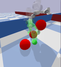
(a)

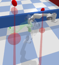
(b)

Figure 6: Examples for simulation setups with panda robot. Initial configuration are shown in white and final configurations in light green. Obstacles are visualized in red. In (a), only static obstacles are considered. In (b), the trajectories of two moving obstacles are visualized in light red.

Simulation

A series of $N=50$ runs was evaluated with the panda robot in simulation. Randomized end-effector positions were set for every run, while the initial configuration remained unchanged. One to five spherical obstacles of radius $r=0.15$ m were placed in the workspace at random. An example setup is shown in Fig. 6(a). The results are summarized in Fig. 7. Solver times with fabrics averaged at $1$ ms while the MPC solver took around $50$ ms in every time step. Although the path length is similar with both solvers, the minimum clearance from obstacles is increased with SF ($0.183$ m) compared to MPC ($0.138$ m). This means that the trajectories are safer and thus more suitable for dynamic environments. Both motion generation methods fail in 6 cases. However, the SF produce only one collision while MPC creates 5 collisions. The remaining failures are deadlocks. For both methods, deadlocks result from local minima, highlighting the need for supportive global plans. Collisions are caused by numerical inaccuracies, which are generally higher with MPC due to the lower frequency.

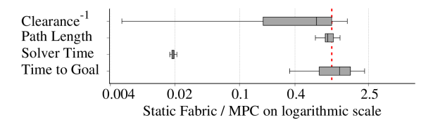
(a) Metrics evaluation for successful experiments

(b) Success results

Figure 7: Results for randomized motion planning problems with the panda robot in simulation. Lower values represent an improved performance of SF over MPC.

Real World

For the experiments with the real robot, we limited the number of test runs to $N=20$. In contrast to the simulated results, MPC has significantly more collisions than SF, Fig. 8(b). This is likely to be caused by the lower frequency at which the MPC is running. While in simulation the model matches the actual behaviour perfectly and the time interval between two computations can be accuratly predicted, more uncertainty in the model is present in the real world. This leads to prediction errors that cause collisions. For the collision free cases, the real world experiments confirm that optimization fabrics tend to be more conservative with respect to obstacles, see Clearance in Fig. 8(a). Similar to the simulated results, the solving time is reduced by a factor of around $50$ with fabrics. This allows to run the planner at a higher frequency and thus generating smoother motions.

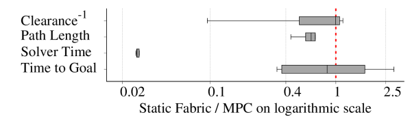
(a) Metrics evaluation for successful experiments

(b) Success results

Figure 8: Results for randomized motion planning problems with the real panda robot. SF are more conservative around obstacles, improving on safety, while reducing the computational cost by a factor of $\approx$ 50. As a result of the increased clearance, collisions are more reliably avoided with SF.

Discussion

The difference in performance (except for solver time) is likely caused by the different objective metrics. The objective function in the MPC formulation is mainly governed by the Euclidean distance to the goal while control inputs and velocity magnitude are given a relative small weight. Avoidance behaviors, such as joint limit avoidance and obstacle avoidance, are respected through inequality constraints. In contrast, SF design the objective in a purely geometric manner including all avoidance behaviors. Thus the manifold for the motion is directly altered by the avoidance behaviors, i.e., the manifold is bent [9] so that the notion of shortest path changes with the addition of obstacles. This shaping of the manifold leads to improved canvergence compared to the combination of Euclidean distance objective function and inequality constraints used with MPC.

VI-C Experiment 2: Static fabrics vs. Dynamic fabrics

In motion planning for dynamic environments, global and local planning methods work together to achieve efficient and safe motion of the robot. However, SF are not designed to follow global paths. Path following can only be achieved using a pseudo-dynamic approach where the forcing potential is shifted in every time step without considering the dynamics of the trajectory. Therefore, we propose DF to allow smoother path following tasks, where the speed of the goal is also considered during execution. In this second experiment, we investigate how DF compare to SF for path following tasks. Specifically, we show that DF outperform SF when following a path generated by a global planner.

Simulation

We evaluated DF on the panda robot robot in simulation with an analytic, time-parameterized curve and a path generated by a global planner, namely RRT (Fig. 9). In the case of the analytic trajectory, the three obstacles were randomized across all runs. For the experiment with the global planner, the goal position and the obstacles were randomized across all runs. A total of $N=50$ experiments were executed for this experiment. The reduced summed error for dynamic fabrics verifies the theoretical finding that dynamic fabrics can follow paths more closely. The average error over all runs with the analytic trajectory is $0.0792$m (DF) and $0.136$m (SF), see Fig. 11(a) for the comparison. For the spline path generated with RRT, the average error over all runs is $0.145$m (DF) and $0.240$m (SF), see Fig. 11(b) for the comparison.

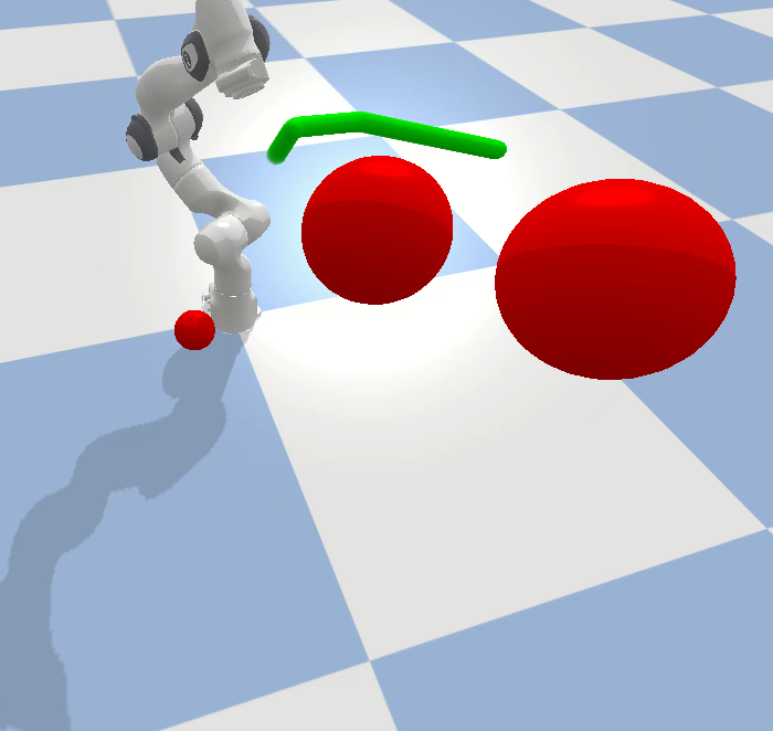
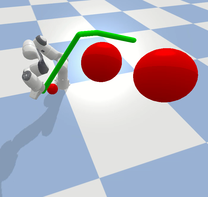
Figure 9: Path generated with RRT from OMPL.

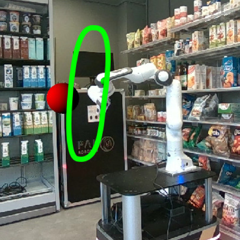
(a)

(b)

Figure 10: Trajectory following tasks with Dynamic Fabrics. In (a), the trajectory is a time-parameterized analytic curve. In (b), the trajectory is described by a spline.

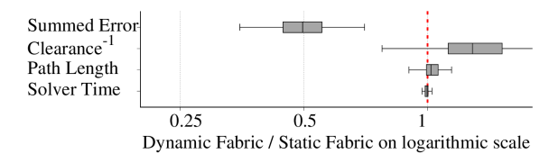
(a) Analytic, user-specified global path

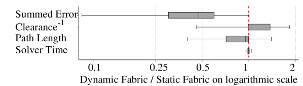
(b) Global path generated by RRT using OMPL

Figure 11: Comparison between static and dynamic fabrics for trajectory following tasks in simulation. Lower values in a metric indicate that DF performed better than SF.

Real-World

Path following was also assessed with the real panda robot in similar settings. Quantitative results are only presented for $N=20$ different paths with splines where up to three obstacles were added to the workspace, see Fig. 10. The results in real-world confirm the findings from the simulation. By exploiting the velocity information of the trajectory, the integration error can be effectively reduced, Fig. 12. In contrast to the simulation we see a higher fluctuation in solver times, which can be caused by a generally lower capacity of the computing unit on the robot.

Figure 12: Comparison between SF and DF when following a path defined by a basic spline in the real world. The splines and the obstacles are different for the $N=20$ case. DF achieve lower deviation errors that SF.

VI-D Experiment 3: Moving Obstacles

Next, we compare the different methods in the presence of dynamic obstacles. All experiments in this section consist of at least one moving obstacle that follows either an analytic trajectory or a spline. Here, we use stationary goals to isolate the results from the behavior investigated in the previous section.

Simulation

For this series with the simulated panda robot, only the goal position was randomized. The initial configuration

$$\bm{q}_{0}={[1.0,0.0,0.0,-1.5,0.0,1.8675]}^{T},$$

and the two moving obstacles with the trajectories

$$\bm{\tilde{x}}_{\textrm{obst1}} ={[-1.0+0.1t,-0.4,0.7]}^{T},$$

$$\bm{\tilde{x}}_{\textrm{obst2}} ={[-1.0+0.2t,1.0-0.1t,0.3]}^{T}$$

were kept constant throughout all experiments. The environment is visualized in Fig. 6(b). The comparison between SF and DF shows that DF are more conservative in terms of collision avoidance with dynamic obstacles. Specifically, the distance between the robot and the obstacles is increased (Fig. 13(a)). The success rate with DF compared to SF is significantly improved, see Fig. 13(b). Thus showing the need for using DF in dynamic environments.

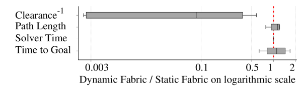
(a) Metrics evaluation for sucessful experiments

(b) Success results

Figure 13: Comparison between SF and DF for scenarios with dynamic obstacles. While path length and solver time is not increased, clearance is increased and the time to reach the goal is reduced with DF compared to SF.

Real-World

In a series of $N=20$ experiments, performance on the real panda arm was assessed. The same trend for more conservative behavior with DF compared to SF can be observed, Fig. 14. However, DF take longer on average to reach the goal as they keep larger clearance from obstacles. Note that collisions are effectively eliminated with DF compared to SF.

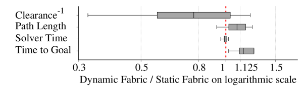
(a) Metrics evaluation for successful experiments

(b) Success results

Figure 14: Comparison between SF and DF for real-world scenarios with dynamic obstacles.

By investigating one example out of the series, see trajectories in Fig. 15, the reason for the large number of collisions with SF can be explained. Both methods initially drive the end-effector to the goal position. As the moving obstacle is approaching the robot, the DF are starting to react while SF are not changing its behavior resulting in a very sudden motion at around $t=30$s. SF treat moving obstacles as pseudo-static (i.e., the position of the obstacle is updated at every time step, but the information on its velocity is discarded). As a result, the relative velocity between obstacle and robot is only a function of the velocity of the robot. Geometries and energies for collision avoidance with fabrics are, by design, a function of this velocity and therefore fail to avoid moving obstacles when the robot moves slowly or not at all. This behavior is most visible when the goal has already been reached but an obstacle is approaching. DF on the other hand take the velocity of the moving obstacles into account and can therefore avoid them.

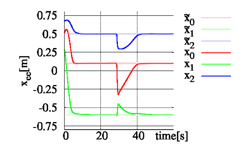
(a) Static Fabric

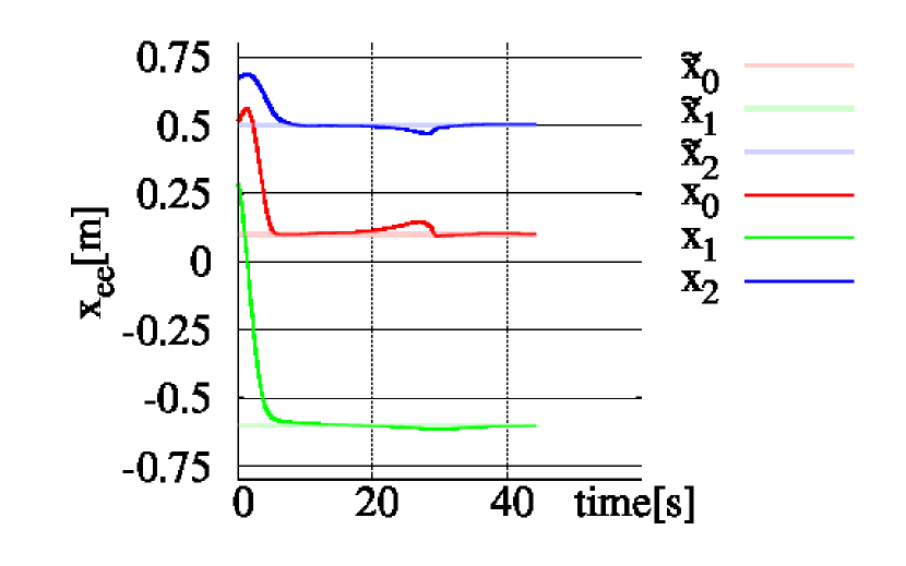
(b) Dynamic Fabric

Figure 15: Trajectories for real panda robot in the presence of a dynamic obstacle. DF show a smoother and in-advance reaction to the approaching obstacle while SF can only react in sudden motion.

VI-E Experiment 4: Nonholonomic robots

Simulation

This experiment assesses the performance of the proposed method to compute trajectories for non-holonomic robots with fabrics. Specifically, we run experiments for a Clearpath Boxer for position. As for the first experiment, we compare the performance to MPC. In this experiment, the initial position, the goal location, and the position of five obstacles were randomized. The results reveal that our extension of optimization fabrics to non-holonomic robots maintains similar results as with a robotic arm. Specifically, computational time can be reduced to optimization-based methods while maintaining good performance in terms of safety and goal-reaching, Fig. 16. We can also observe that success rate with SF is lower compare to MPC due to a high number of unreached goals.

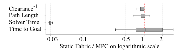
(a) Metrics evaluation for successful experiments

(b) Success results

Figure 16: Results for randomized cased with the Clearpath Boxer robot. Similar performance in terms of safety and goal-reaching can be combined with very fast computation using optimization fabrics.

VI-F Experiment 5: Mobile manipulators

In the final experiment, we assess the applicability of SF and DF to a non-holonomic mobile manipulator. In an environment that is densely occluded by obstacles, the motion planning problem is defined by a desired end-effector position and additional path constraints (e.g. desired orientation of the end-effector).

Simulation

In simulation, we evaluate the performance of our extension to non-holonomic mobile manipulators with SF. In this series, the positions of 8 obstacles are randomized for $N=50$ cases. The workspace was limited to a 7mx7m square, so that random obstacles are ensured to be actually hindering the motion planner. The results reveal that properties shown in the previous experiments transfer to more complex systems without loss of the computational benefit, Fig. 17. In this series, there were 1 unreached goals and 4 collisions which are, similar to the previous experiments, caused by local minima. Local minima are more likely for mobile manipulators as their workspace is larger.

Figure 17: Quantitative results with static fabrics for a non-holonomic mobile manipulator in simulation. Fabrics solve planning problems in randomized environments in low planning time. This allows whole-body control and highly reactive behavior.

Combining our contributions, DF and the extension to non-holonomic robots, we achieve reactive and safe behavior in dynamic environments. Moving obstacles are avoided in a natural way using our method, see Fig. 18.

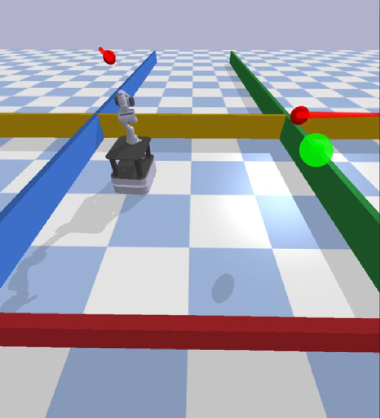
(a) $t=0$s

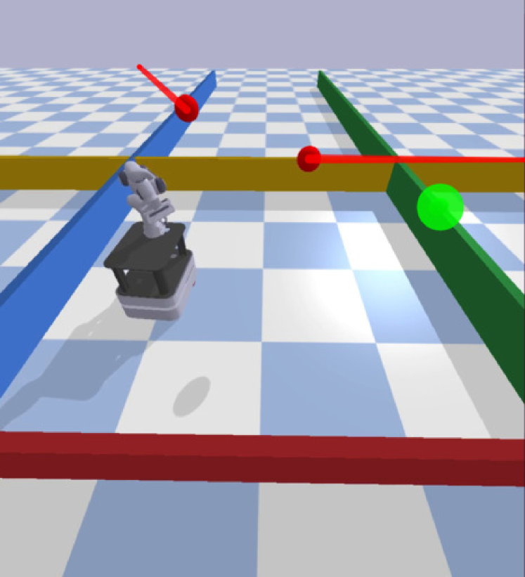
(b) $t=7$s

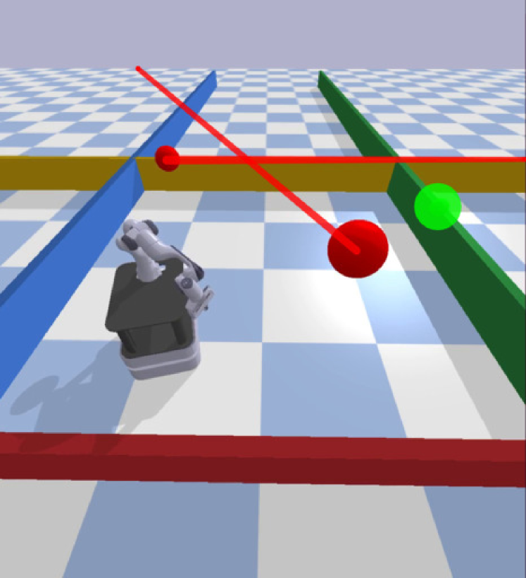
(c) $t=14$s

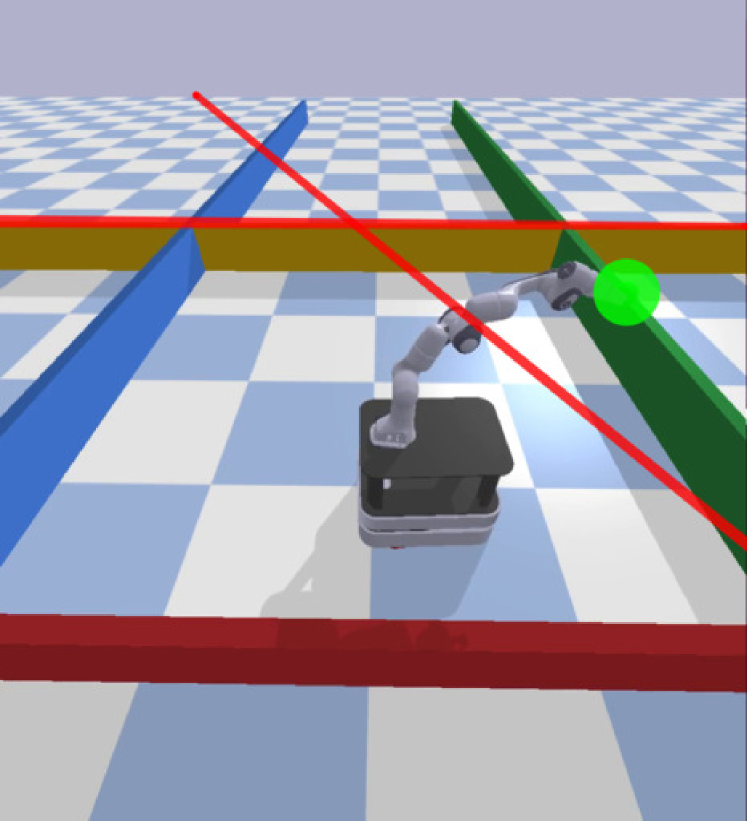
(d) $t=20$s

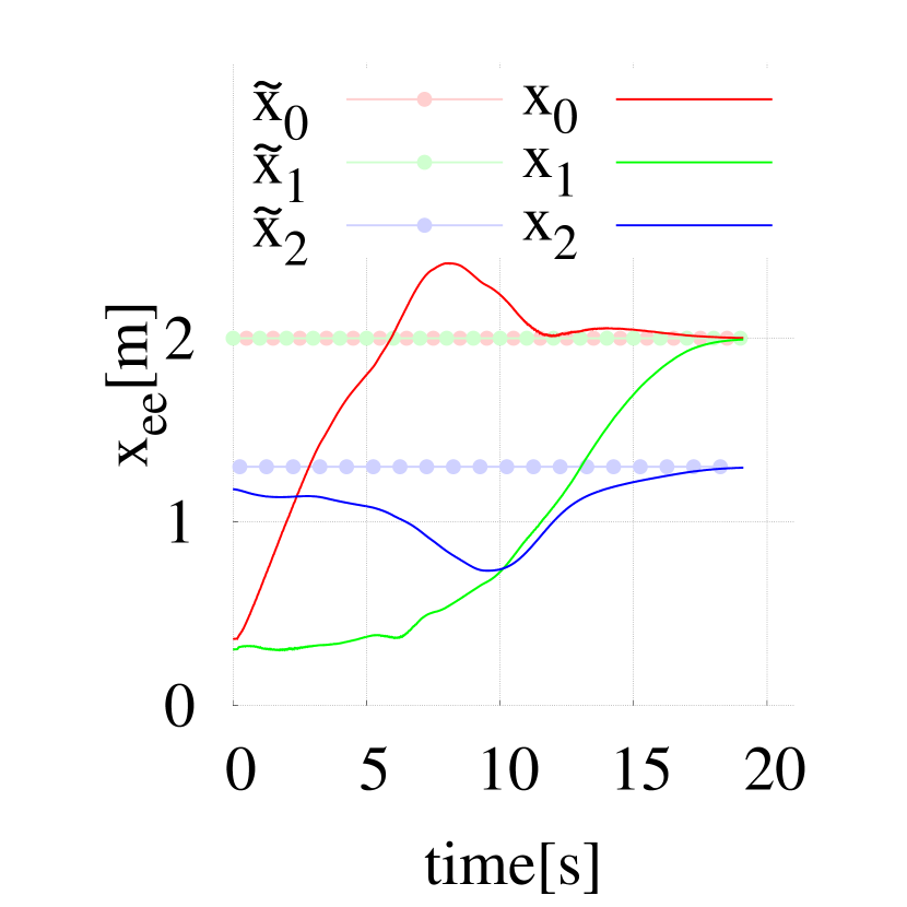
(e)

Figure 18: Sequence of trajectory computed with DF for a mobile manipulator in simulation with moving obstacles (red sphere with line indicating the past trajectory) and one end-effector goal (green). The trajectory of the end-effector are visualized in (e) as $\bm{x}$ and the desired end-effector position as $\bm{\tilde{x}}$.

Real-World

We present qualitative results for a non-holonomic mobile manipulator using DF. In Fig. 1, the robot follows a trajectory defined by a basic spline, while additionally respecting an orientation constraints on its end-effector and avoiding the shelves and an obstacle on the ground. The end-effector trajectory is plotted in Fig. 19.

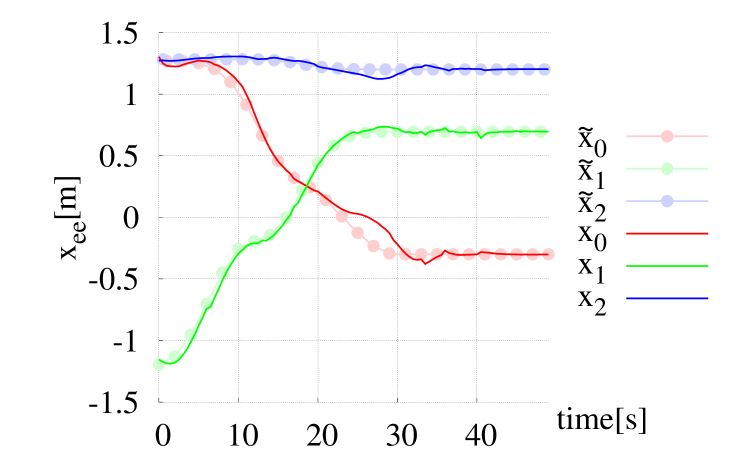
Figure 19: Real-world experiment for path following with a mobile manipulator. The global path can be tracked accurately by DF including the extension to non-holonomic robots. The scene is visualized in Fig. 1.

VI-G Experiment 6: Dynamic fabrics in supermarkets

In this experiment, we show qualitatively how DF could be used in collaborative environments where humans and robots coexist. For this experiment, we give the robot a static goal pose similar to a pickup setup. The same environment is shared with a co-worker who restocks a shelf. The right hand of the human is tracked with a motion capture system. The hand is then avoided by the robot using DF, see Fig. 19. In this experiment, the minimum distance between the robot and the hand was $0.062$m. This real-world experiment showcases potential applications of the proposed method.

VII Conclusion

In this paper, we have generalized optimization fabrics to dynamic environments. We have proven that our proposed Dynamic Fabrics are convergent to reference paths and can thus compute motion for path following tasks (Lemma IV.10). Besides, we have proposed an extension to optimization fabrics (and thus also DF) for non-holonomic robots. This allows the application of this framework to a wider range of robotic applications and ultimately allows the deployment to many mobile manipulators in dynamic environments.

These theoretical findings were confirmed in various experiments. First, the quantitative comparisons showed that Static Fabrics outperforms MPC in terms of solver time while maintaining similar performance in terms of goal-reaching and success rate. The improved performance with optimization fabrics might be caused by the different metric for goal reaching compared to Model Predictive Control. An integration of non-Riemannian metrics into an MPC formulation should be further investigated in the future.

Verifying our theoretical derivations for DF, the experiments showed that the deviation error for path following tasks is decreased compared to SF. Similarly, environments with moving obstacles and humans showed increased clearance while maintaining low computational costs and execution times. Thus, DF overcome an important drawback of SF [9, 10], where collision avoidance with moving obstacle is solved purely by the high frequency at which optimization fabrics can be computed. Moreover, the generalization did not increase the solving time compared to SF. Unlike the original work on optimization fabrics, this generalization allows the deployment to dynamic environments where velocity estimates of moving obstacles are available.

Direct sensor integration in optimization fabrics might be feasible in future works to overcome the shortcomings of perception pipelines for collision avoidance. For the trajectory path tasks in this paper, we used a simple global path generated in workspace. As DF integrate global path in arbitrary manifolds, improving the global planning phase could be further investigated. We expect this to be beneficial when robotics tasks are constantly changing and task planning is required.

Max Spahn received the B.Sc. degree in Mechanical Engineering at the RWTH Aachen in 2018. He received his M.Sc. in General Mechanical Engineering at the RWTH in 2019. He also received the degree Diploma d‘ingenieur de Centrale Supelec in 2020 as part of a double degree program. He is currently working towards his Ph.D. degree in robotics. Furthermore, he is part of AIRLab, the AI for Retail Lab in Delft. His research interests in geometric approaches to motion planning and trajectory generation. He is passionate about open-sourcing scientific code, as he believes it will improve scientific outcome in robotics.

Martijn Wisse received the M.Sc. and Ph.D. degrees in mechanical engineering from the Delft University of Technology, Delft, The Netherlands, in 2000 and 2004, respectively. He is currently a Professor at the Delft University of Technology. His previous research focused on passive dynamic walking robots and passive stability in the field of robot manipulators. He worked on underactuated grasping, open-loop stable manipulator control, design of robotic systems, and the creation of startups in this field. His current research interests focus on the neuroscientific principle of active inference and its application and advancements in robotics.

Javier Alonso-Mora is an Associate Professor at the Delft University of Technology, where he leads the Autonomous Multi-robots Lab. He received his Ph.D. degree in robotics from ETH Zurich, in partnership with Disney Research Zurich, and he was a Postdoctoral Associate at the Computer Science and Artificial Intelligence Lab (CSAIL) of the Massachusetts Institute of Technology. His research focuses on navigation, motion planning, and control of autonomous mobile robots, with a special emphasis on multi-robot systems, mobile manipulation, on-demand transportation, and robots that interact with other robots and humans in dynamic and uncertain environments. He currently serves as associate editor for IEEE Transactions on Robotics and for Springer Autonomous Robots. He is the recipient of a talent scheme VENI award from the Netherlands Organization for Scientific Research (2017), the ICRA Best Paper Award on Multi-robot Systems (2019) and an ERC Starting Grant (2021).

References

- [1] S. Karaman and E. Frazzoli, “Sampling-based algorithms for optimal motion planning,” in International Journal of Robotics Research, vol. 30, no. 7, jun 2011, pp. 846–894. [Online]. Available: http://journals.sagepub.com/doi/10.1177/0278364911406761
- [2] D. Hrovat, S. Di Cairano, H. Tseng, and I. Kolmanovsky, “The development of model predictive control in automotive industry: A survey,” in 2012 IEEE International Conference on Control Applications, 2012, pp. 295–302.
- [3] M. Bujarbaruah, X. Zhang, F. Borrelli, and H. Eric Tseng, “Learning-Based Model Predictive Control: Toward Safe Learning in Control,” pp. 269–296, 2018. [Online]. Available: https://doi.org/10.1146/annurev-control-090419-
- [4] M. Bednarczyk, H. Omran, and B. Bayle, “Model Predictive Impedance Control,” in Proceedings - IEEE International Conference on Robotics and Automation. Institute of Electrical and Electronics Engineers Inc., may 2020, pp. 4702–4708.
- [5] S. Richter, S. Mariéthoz, and M. Morari, “High-speed online MPC based on a fast gradient method applied to power converter control,” in Proceedings of the 2010 American Control Conference, ACC 2010. IEEE Computer Society, 2010, pp. 4737–4743.
- [6] M. Xie, K. Van Wyk, A. Li, M. A. Rana, Q. Wan, D. Fox, B. Boots, and N. Ratliff, “Geometric Fabrics for the Acceleration-based Design of Robotic Motion,” oct 2020. [Online]. Available: http://arxiv.org/abs/2010.14750
- [7] W. Edwards, G. Tang, G. Mamakoukas, T. Murphey, and K. Hauser, “Automatic tuning for data-driven model predictive control,” in 2021 IEEE International Conference on Robotics and Automation (ICRA), 2021, pp. 7379–7385.
- [8] C. A. Cheng, M. Mukadam, J. Issac, S. Birchfield, D. Fox, B. Boots, and N. Ratliff, “RMPflow: A computational graph for automatic motion policy generation,” 2018.
- [9] N. D. Ratliff, K. Van Wyk, M. Xie, A. Li, and M. A. Rana, “Optimization fabrics,” arXiv preprint arXiv:2008.02399, 2020.
- [10] K. Van Wyk, M. Xie, A. Li, M. A. Rana, B. Babich, B. Peele, Q. Wan, I. Akinola, B. Sundaralingam, D. Fox et al., “Geometric fabrics: Generalizing classical mechanics to capture the physics of behavior,” IEEE Robotics and Automation Letters, 2022.
- [11] C.-A. Cheng, M. Mukadam, J. Issac, S. Birchfield, D. Fox, B. Boots, and N. Ratliff, “RMPflow: A Geometric Framework for Generation of Multi-Task Motion Policies,” Tech. Rep., 2020.
- [12] M. Rickert, A. Sieverling, and O. Brock, “Balancing exploration and exploitation in sampling-based motion planning,” IEEE Transactions on Robotics, vol. 30, no. 6, pp. 1305–1317, dec 2014.
- [13] M. Stilman, “Global manipulation planning in robot joint space with task constraints,” IEEE Transactions on Robotics, vol. 26, no. 3, pp. 576–584, jun 2010.
- [14] D. Berenson, S. Srinivasa, and J. Kuffner, “Task Space Regions: A framework for pose-constrained manipulation planning,” International Journal of Robotics Research, vol. 30, no. 12, pp. 1435–1460, oct 2011.
- [15] Z. Kingston, M. Moll, and L. E. Kavraki, “Exploring implicit spaces for constrained sampling-based planning,” International Journal of Robotics Research, vol. 38, no. 10-11, pp. 1151–1178, 2019.
- [16] A. H. Qureshi, J. Dong, A. Baig, and M. C. Yip, “Constrained Motion Planning Networks X,” 2020. [Online]. Available: http://arxiv.org/abs/2010.08707
- [17] B. Brito, B. Floor, L. Ferranti, and J. Alonso-Mora, “Model Predictive Contouring Control for Collision Avoidance in Unstructured Dynamic Environments,” IEEE Robotics and Automation Letters, vol. 4, no. 4, pp. 4459–4466, 2019.
- [18] D. Mayne, J. Rawlings, C. Rao, and P. Scokaert, “Constrained model predictive control: Stability and optimality,” Automatica, vol. 36, no. 6, pp. 789–814, Jun. 2000. [Online]. Available: https://linkinghub.elsevier.com/retrieve/pii/S0005109899002149
- [19] A. W. Winkler, C. D. Bellicoso, M. Hutter, and J. Buchli, “Gait and Trajectory Optimization for Legged Systems Through Phase-Based End-Effector Parameterization,” IEEE Robotics and Automation Letters, vol. 3, no. 3, pp. 1560–1567, Jul. 2018. [Online]. Available: http://ieeexplore.ieee.org/document/8283570/
- [20] S. S. Keerthi and E. G. Gilbert, “Optimal infinite-horizon feedback laws for a general class of constrained discrete-time systems: Stability and moving-horizon approximations,” Journal of optimization theory and applications, vol. 57, no. 2, pp. 265–293, 1988.
- [21] J. Tordesillas, B. T. Lopez, and J. P. How, “FASTER: Fast and Safe Trajectory Planner for Flights in Unknown Environments,” in IEEE International Conference on Intelligent Robots and Systems, 2019, pp. 1934–1940. [Online]. Available: https://github.com/jtorde
- [22] G. B. Avanzini, A. M. Zanchettin, and P. Rocco, “Constraint-based Model Predictive Control for holonomic mobile manipulators,” in IEEE International Conference on Intelligent Robots and Systems, vol. 2015-Decem. Institute of Electrical and Electronics Engineers Inc., dec 2015, pp. 1473–1479.
- [23] G. Buizza Avanzini, A. M. Zanchettin, and P. Rocco, “Constrained model predictive control for mobile robotic manipulators,” pp. 19–38, 2018. [Online]. Available: https://doi.org/10.1017/S0263574717000133
- [24] M. Spahn, B. Brito, and J. Alonso-Mora, “Coupled mobile manipulation via trajectory optimization with free space decomposition,” in 2021 IEEE International Conference on Robotics and Automation (ICRA). IEEE, 2021, pp. 12 759–12 765.
- [25] I. R. Manchester and J.-J. E. Slotine, “Control Contraction Metrics: Convex and Intrinsic Criteria for Nonlinear Feedback Design,” IEEE Transactions on Automatic Control, vol. 62, no. 6, pp. 3046–3053, Jun. 2017. [Online]. Available: http://ieeexplore.ieee.org/document/7852456/
- [26] B. Yi, R. Wang, and I. R. Manchester, “On necessary conditions of tracking control for nonlinear systems via contraction analysis,” Nov. 2020, arXiv:2009.08662 [cs, eess]. [Online]. Available: http://arxiv.org/abs/2009.08662
- [27] O. Khatib, “A Unified Approach for Motion and Force Control of Robot Manipulators: The Operational Space Formulation,” IEEE Journal on Robotics and Automation, vol. 3, no. 1, pp. 43–53, 1987.
- [28] N. D. Ratliff, J. Issac, D. Kappler, S. Birchfield, and D. Fox, “Riemannian motion policies,” jan 2018. [Online]. Available: http://arxiv.org/abs/1801.02854
- [29] X. Meng, N. Ratliff, Y. Xiang, and D. Fox, “Neural autonomous navigation with riemannian motion policy,” in Proceedings - IEEE International Conference on Robotics and Automation, vol. 2019-May. Institute of Electrical and Electronics Engineers Inc., may 2019, pp. 8860–8866.
- [30] N. D. Ratliff, K. Van Wyk, M. Xie, A. Li, and M. A. Rana, “Generalized nonlinear and finsler geometry for robotics,” in 2021 IEEE International Conference on Robotics and Automation (ICRA). IEEE, 2021, pp. 10 206–10 212.
- [31] M. Bhardwaj, B. Sundaralingam, A. Mousavian, N. Ratliff, D. Fox, F. Ramos, and B. Boots, “STORM: An Integrated Framework for Fast Joint-Space Model-Predictive Control for Reactive Manipulation,” 2021. [Online]. Available: http://arxiv.org/abs/2104.13542
- [32] C.-A. Cheng, M. Mukadam, J. Issac, S. Birchfield, D. Fox, B. Boots, and N. Ratliff, “RMPflow: A Geometric Framework for Generation of Multi-Task Motion Policies,” Tech. Rep., 2020.
- [33] M. Spahn, C. Salmi, and J. Alonso-Mora, “Local planner bench: Benchmarking for local motion planning,” arXiv preprint arXiv:2210.06033, 2022.
- [34] C. Meo, G. Franzese, C. Pezzato, M. Spahn, and P. Lanillos, “Adaptation through prediction: multisensory active inference torque control,” arXiv preprint arXiv:2112.06752, 2021.
- [35] A. Domahidi and J. Jerez, “Forces professional,” Embotech AG, url=https://embotech.com/FORCES-Pro, 2014–2019.
- [36] A. Zanelli, A. Domahidi, J. Jerez, and M. Morari, “Forces nlp: an efficient implementation of interior-point… methods for multistage nonlinear nonconvex programs,” International Journal of Control, pp. 1–17, 2017.