Cyber Risk Assessment for Capital Management

Abstract

Cyber risk is an omnipresent risk in the increasingly digitized world that is known to be difficult to manage. This paper proposes a two-pillar cyber risk management framework to address such difficulty. The first pillar, cyber risk assessment, blends the frequency-severity model in insurance with the cascade model in cybersecurity, to capture the unique feature of cyber risk. The second pillar, cyber capital management, provides informative decision-making on a balanced cyber risk management strategy, which includes cybersecurity investments, insurance coverage, and reserves. This framework is demonstrated by a case study based on a historical cyber incident dataset, which shows that a comprehensive cost-benefit analysis is necessary for a budget-constrained company with competing objectives for cyber risk management. Sensitivity analysis also illustrates that the best strategy depends on various factors, such as the amount of cybersecurity investments and the effectiveness of cybersecurity controls.

Keywords: cyber risk assessment, cyber capital management, cascade model, cybersecurity investment, insurance coverage and reserve.

1 Introduction

As modern businesses and public-sector entities have become greatly reliant on information technology (IT) to boost the efficiency of workflows and stay connected with the world, potential cyber incidents, such as data breaches, pose great dangers to organizations’ daily operations. Therefore, managing cyber risk should be a critical component in enterprise risk management practices.

1.1 Difficulties in cyber risk management

A successful cyber risk management plan should include both a risk assessment component and a capital allocation component, as noted in [36] regarding how to establish or improve a cybersecurity program and how to make buying decisions. In practice, neither of the two tasks is trivial.

Regarding the risk assessment aspect, as an emerging type of risk, cyber risk is more difficult to assess than many other traditional risks for reasons including the following.

• Lack of quantitative tools for comprehensive cyber risk assessment. Although there are lots of efforts in quantifying some aspects of cyber risks, such as the impact of data breaches (see, for example, [47, 21]), it should be recognized that cyber systems consist of numerous types of physical and virtual components, and they may have drastically different risk exposures. In order to guide business decisions on cyber risk management, a comprehensive and quantitative assessment of the risk that integrates all those components is crucial. Still, the tool for such a purpose is lacking in the literature.

• Adaptive nature of cyber risk. As summarized in [16], cyber risk is dynamic in the sense that in cyberspace, adversaries are consistently developing new strategies and attacks to overcome or bypass existing defense mechanisms. In other words, even a well-protected system by today’s cybersecurity technology may still be vulnerable again in the future time. Therefore, an ideal framework for cyber risk assessment has to take both internal factors, such as security measures, and external factors, such as trending attacking techniques, into account. The latter component is usually missing in many existing risk assessment approaches.

• Correlated losses. It is well-known that because of the connectedness of cyberspace, cyber risks are correlated. [6] discussed two modes of correlation, namely intra-firm risk correlation and global risk correlation. From the perspective of a decision-maker, who manages the cyber risk of a particular company, the intra-firm correlation is more of a concern. That is, a single cyber incident may result in multiple points of failure, each of which can lead to a loss; see, for example, [2]. Such a dependence relationship among losses can be obscure and easily overlooked by risk managers.

Beyond the cyber risk assessment, another critical challenge faced by risk managers in an enterprise environment is prioritizing and combining different risk management tools, including risk reduction, transfer, and retention, which further leads to making buying decisions in the implementation stage of the risk management program. To reduce cyber risk, a company should implement cybersecurity controls, which often involve purchasing cybersecurity solutions and hiring security experts. To transfer the reduced risk, the company should consider buying cyber insurance coverage for specific perils and losses. To retain the reduced but uncovered risk, the company needs an emergency fund to mitigate the impact of an incident to ensure business continuity. These risk management options all bear costs. However, the amount of capital that can be budgeted for managing cyber risk is often limited, thus making developing a cost-efficient capital allocation strategy for effective cyber risk management a complex task for enterprises.

This paper proposes a two-pillar cyber risk management framework that addresses the above challenges in cyber risk assessment and capital allocation. The first pillar, cyber risk assessment, utilizes a cascade risk arrival model that unifies the three key components in cybersecurity, including threats, vulnerabilities, and assets, to fully account for the dynamics of cyber risk and the intra-firm loss correlations. The second pillar, cyber capital management, solves for the optimal amounts of capital assigned to various types of risk management devices, such that the overall magnitude of costs and losses is minimized.

Given that cyber risk management is an interdisciplinary subject, the proposed framework takes advantage of approaches to this problem developed by both the cybersecurity community and the actuarial and economics community, which shall be reviewed and compared in the following subsections.

1.2 Cybersecurity, actuarial, and economics approaches to cyber risk

Developing innovative risk assessment methods to address the above-mentioned difficulties is interesting to both cybersecurity and risk management communities. Focusing on different aspects of cyber risks, those two communities have developed vastly different approaches to cyber risk assessment and management.

Cybersecurity approach

In the cybersecurity literature, researchers often focus on the structural properties of cyber systems and study the risks at a microscopic level. For example, [45] discussed security issues associated with smart grids with extensive insights into the vulnerabilities in individual components of the network and then proposed countermeasures to potential threats, including various attack detection mechanisms and attack mitigation approaches targeting network and physical layers. Those insights are helpful for smart grid operators to identify risks and build a list of action items for risk mitigation. A similar approach is taken in [22] to identify and reduce risks in Internet-of-Things (IoT) systems. The authors identified that the perception layer of physical sensors is the most vulnerable part of an IoT system and proposed a score-based risk assessment method for critical security issues.

Based on the same methodology but for more generalized use cases in industrial environments, regulators and leaders of the cybersecurity industry have developed a handful of guidelines and frameworks. For example, the National Institute of Standards and Technology (NIST) has developed a generic set of controls called the Cybersecurity Framework (CSF) (see [36]), which can be used by organizations as voluntary guidance for cyber risk management. Similarly, as a cybersecurity industry leader, the Center for Internet Security (CIS) has compiled a detailed list of commonly known vulnerable components in cyber systems and best practices in risk mitigation into CIS Controls (see [13]).

In terms of their practicality, one potential shortcoming of these is the lack of insight into the prioritization of tasks from the cost-benefit perspective. For example, Security and Privacy Controls for Federal Information Systems and Organizations (known as SP 800-53) is a core component in NIST CSF (see [36]), and although it assigns priority codes to security controls, as clarified in the document, those codes are for implementation sequencing that is reasoned from the cybersecurity perspective, but they provide no information on whether implementing a certain control is economically beneficial. Except for the entities who are subject to the requirements in SP 800-53, other organizations may find such guidelines not instructive enough on how to allocate capital for these security controls. As mentioned in [25], private-sector firms have other investment decisions than cybersecurity, and they all compete for limited organizational resources. For this reason, cost-benefit analysis is important in the decision-making process regarding cybersecurity investment.

Overall, cybersecurity approaches mainly focus on infrastructural details but may not provide enough support for strategic investment and capital allocation planning. The capital component in cyber risk management is largely missing in mainstream solutions provided by the engineering community.

Actuarial and economics literature

In the actuarial literature, more emphasis is on the losses caused by cyber incidents, while cyber systems are often highly abstracted. For example, [33] modeled a power system as a collection of nodes and modeled the dynamics of an attack on that system using an absorbing semi-Markov process, which further led to discussions on the financial consequences of cyber threats. [21] studied a dataset that contains historical cyber losses, identified classes of cyber risks depending on causes, such as human error or technical failure, and then modeled loss frequency and severity by probability distributions. [20] studied a collection of historical data breaches and used vine copulas to model the dependence among cyber losses in terms of the number of breached records. Using the same dataset of data breaches, [47] performed trend analyses and built stochastic models for the frequency and size of data breaches caused by hacking. In the economics literature, [31] combined the information on past data breaches and the impacted firms from multiple sources and showed that the frequency of attacks and the size of cyber losses are influenced by various factors, such as the existence of a risk oversight committee and the type of the breached information. More broadly, some studies focus on the impacts of cyber incidents on the economy. [19] showed that the damage caused by cyber-attacks to different banking industry participants could be spread to other entities in the industry through the payments system, thus enlarging the loss. [17] found that small data breaches in the financial and insurance services industry tended to have negative spillover effects on cyber insurance providers, whereas some extremely large ones could lead to increased risk awareness, thus resulting in a positive effect.

Many of the studies from the actuarial and economics perspectives help understand the consequences of cyber incidents, thus providing organizations with suggestions on how to prepare for potential losses resulting from various types of cyber incidents. There are also several economics studies that try to draw connections between cyber losses and cybersecurity practices, such as how losses can be reduced by implementing certain security controls. For example, [24, 31] proposed various models for calculating the optimal level of investment. In [24], the models express the probability of experiencing a security breach as a function of security investment and then use this probability to calculate the expected loss. The optimal investment in cybersecurity is thus obtained when the marginal investment equals the marginal reduction in expected loss. [40] formulated investment in cybersecurity as an optimization problem, known as the knapsack problem, where there is a target to protect, a fixed budget, and a set of cyber resources that each can be invested in and generates a return, i.e., some level of protection for the target. The goal is to maximize the overall return with the limited budget. The authors also proposed some variants to this problem, where there could be interactions between resources, e.g., one could be an alternative of the combination of another two resources in terms of the generated return, and where there could be multiple targets to protect. These studies provide some insights into the question on how much should be spent on cybersecurity based on the principle that there should be an equilibrium in the trade-off between cyber investment and the residual cyber risk. That is, a decision maker can choose to either spend more on cybersecurity investment and less on the capital reserved for cyber losses, or the other way around.

To generalize this problem a little more, we can see it as the trade-off between the immediate cost and the potential cost in the future. This type of problem is commonplace in the economics literature on topics other than cyber.

For example, the well-known Laffer curve suggests that if a government sets a high tax rate, the initial revenue from taxation may be large, but because of the low profitability, companies may reduce economic activities and the economy may contract, thus leading to low tax revenue. On the contrary, if there is a low tax rate, companies increase production and the economy expands due to higher profitability, thus leading to an expanded source of revenue in the future (see [46]). Clearly, the government needs to strike a balance between the immediate tax income and the income in the long run. Other than taxation, the Laffer curve effect has been studied and applied in many different fields as well; see, for example, [41, 30]. The analog of the Laffer curve is introduced in this paper in the context of cyber risk assessment to explain the trade-off between cybersecurity investment and capitals needed to transfer and absorb the losses.

From a risk perspective, the future benefit could be the reduction in the probability of the occurrence of a loss event. [35] considers a two-period scenario, in which an investment in effort is made today to reduce the probability of a loss tomorrow, and studies how agents with different prudence levels choose their optimal invested efforts. [29] offers an extension to that study, and shows how the curvature of utility and the presence of endogenous saving affect an agent’s choice of investing in either reducing the loss probability or reducing the potential loss size.

Ideally, the thought process for investments in cyber should also include the consideration for benefits. However, as found in [1], organizations rarely incorporate this type of cost-benefit analysis in cyber risk management. What might hinder the development of such strategies is that the existing studies, such as [24, 40], provide no identification of specific cyber assets and vulnerabilities. When multiple vulnerabilities and sources of losses are of concern, the lack of structural information on cyber systems can make it difficult for organizations to create actionable plans and put specific controls in place.

Remarks on comparing classic approaches to frequency, severity, and dependence among cyber losses

Risks are typically modeled by their frequency and severity in actuarial works, and such attempts have also been made for cyber risk assessment (see, for example, [47, 21]), where probability distributions are fitted for the occurrences and sizes of cyber losses, and economic insights into the landscape of cyber risks are derived. However, due to the lack of data at a granular level on how cybersecurity investments can impact those distributions, the managerial implications of the classic approach are often limited. Therefore, in our study, the frequency and severity approach is still adopted, as illustrated in Section 4, but embedded in a comprehensive framework with the structural information of a cyber system that allows for modeling the effect of interventions.

Similarly, statistical approaches have been used to model the dependence among cyber losses, such as copulas (see, for example, [28, 37, 20]). The utility of these models, especially the parameter-rich ones such as vine copulas, is also largely restricted by the low data availability, and these models can be non-informative at the company level and difficult to guide decision-making with respect to enterprise cyber risk management. Therefore, instead of taking a statistical approach, we utilize the structural information of a cyber system to show how multiple points of failure are logically connected, thus causing correlated losses within a company. This shall be elaborated in Section 2.

1.3 Capital management framework for cyber risk and contributions

Comparing the approaches taken by these two communities, solutions to specific cybersecurity challenges are usually the focus of engineering research, whereas the economics and finance community typically emphasizes the outcomes of cyber incidents. The former offers instructions on addressing specific cyber threats by implementing certain security controls, and the latter generates economic incentives for organizations to take actions to reduce the risk. However, we are unaware of any unified solution that takes benefit of both perspectives. Imagine that an organization is considering investing in a set of CIS Controls. To make this management decision, it needs to assess how much loss reduction can be achieved by implementing those controls and determine how much should be invested in each. These questions are non-trivial and yet to be answered.

To guide business decisions on cyber risk management, we propose a framework that quantifies the relationship between the structural information of a cyber system and various kinds of cyber risks that may arise from this system via a cascade risk arrival model. It sets out the amount of risk borne by individual vulnerabilities and assets, and this detailed risk assessment further allows for budgeting decisions regarding cyber risk management. Specifically, this framework optimizes for the amount of capital allocated to various risk management tools, including:

• Ex-ante investment, which is the investment in implementing security controls, such as hiring cybersecurity professionals, applying security patches, and training personnel, and it has an immediate effect on reducing cyber risk exposure before any incidents happen. In this paper, we assume that the company has already implemented some controls which match the industry-average security standard, and our discussions on cybersecurity investments surround any additional spending on top of that level.

• Cyber insurance, which is a device for businesses to transfer their cyber risks to insurers. Cyber insurance policies typically provide coverage for losses resulting from various perils, such as forensics costs, costs for repairing or replacing cyber assets, and legal liabilities in case of lawsuits. Insurers demand premium payments in exchange for the provided coverage.

• Ex-post-loss reserve, which is the emergency fund set up to cover residual losses not indemnified by cyber insurance. Note that this fund is indeed reserved before any cyber incidents happen, but it is then used to absorb losses after the incidents, which explains its ex-post-loss effect.

These three components represent the reduction, transfer, and retention of cyber risk, respectively, and thus the proposed framework is a comprehensive package for the management of cyber risk. It should be pointed out that the interactions among these risk management approaches have been studied in other scholarly works, such as [4, 48, 5, 18], but they typically do not consider this problem in a capital allocation setting. For example, based on a game-theoretic model, [48] discusses how an insurer, acting as a risk reduction services provider at the same time, should price such services.

Our approach takes all three components into consideration and finds an optimal strategy for businesses to allocate their budgets to implementing various cyber controls and preparing for potential future losses. The goal is to minimize the overall cost, which consists of the costs of cybersecurity controls, insurance, and reserves, as well as the impact of cyber losses.

The main contribution of this paper is five-fold.

• This paper presents the first quantitative description of the cascade model previously known in the cybersecurity literature, to the best knowledge of authors. It bridges the gap between the cybersecurity approach and the actuarial and economics approach to cyber risk assessment by providing a unifying framework. The new approach utilizes both the structural information of cyber systems and historical cyber loss data to provide risk assessment and management insights that are quantitative and specific to individual components in cyber systems.

• The framework is compatible and can be implemented along with the existing standards for cybersecurity, such as the NIST CSF. This feature is important for the practicality of a cyber risk management method, but is generally missing in the quantitative methods that have been proposed. Therefore, our work offers a pragmatic tool for decision-making in the process of complying with industry regulations and standards of practice.

• The framework addresses the three aforementioned challenges in cyber risk assessment. Not limited to any specific type of risk, it incorporates the quantitative assessment of potential losses that may arise from various points of failure in a cyber system. In addition, the framework considers both external threats and internal vulnerabilities and assets, so that when a new threat emerges due to the adaptive nature of cyber risk, the model can be easily updated to reflect such a change in the environment. Various cyber components are linked in this framework via attack paths, and that captures the dependence among the risk exposures of them.

• The framework has a capital allocation component that enables users to quantify and assess the trade-off among cybersecurity investment, cyber insurance, and loss reserve. The proposed framework extends the classic security investment model in [24] by accounting for components in cyber systems at a granular level and considering alternative risk management devices, including insurance and reserves.

• The paper presents a novel application of collective risk modeling and Pareto optimization, which are rarely discussed in the context of cyber risk. It presents that for cyber risk management in a business environment, there are competing priorities and objectives, and those techniques are well-suited for such a problem.

The proposed risk assessment and capital allocation methods are implemented in R language, which can be found in the supplementary materials of this paper. Its practicality is demonstrated with real data. Practitioners may easily adopt the computer program for their company-specific applications.

The overall organization of the rest of this paper is as follows. Section 2 proposes a tensor-based loss model for cyber risk assessment, which incorporates the structural information of risk arrival. Based on the risk assessment results, Section 3 introduces the holistic framework of optimizing capital allocation for cybersecurity investment, cyber insurance, and loss reserve. Section 4 provides a case study that integrates the risk assessment process and the decision-making of capital allocation for cyber risk management. Section 5 concludes and outlines some potential future directions.

2 Cyber Risk Assessment

2.1 Cascade model

[7] developed a cascade model to describe the arrival of a cyber incident, in which each arrival process is summarized as follows.

1. Once a threat is initiated by an attacker, it will exploit vulnerabilities in a cyber system.

2. The vulnerabilities that are not fully eliminated by security controls will then be the viable paths for the threat to impact assets in the system.

3. Eventually, assets of different types and values will generate distinct impacts.

This cascade model was developed to explain the process of risk arrival in a cyber system, but was not purposed for the direct quantitative assessment of cyber risks in [7]. In this paper, we take inspiration from this model and extend it to cyber risk assessment, and subsequently cyber capital management in the next section. As summarized in the arrival process, there are five essential cascade components in the model; we shall first explain their details below and use examples to allude to the relationship among them.

• A threat is an action that has the potential to cause damage to a cyber system. They might be initiated externally by hackers or cyber criminals with malicious intent, or they could simply be reckless actions performed internally which lead to unintentional damage. For instance, a common threat for password-protected accounts is an external dictionary attack, which utilizes a large pool of possible passwords to guess the correct one by trial and error until succeeding. As another example of threats, the spread of viruses may cause correlated losses among multiple organizations (see, for example, [14]). Given that this paper focuses on managing the cyber risk of a single organization, this scenario of contamination that leads to a global risk correlation can be treated in the same way as other threats from the single organization’s perspective.

• A vulnerability is a cyber weakness that may be exploited by a threat. A threat alone cannot induce any harm if it fails to match any vulnerabilities in the system. For example, allowing an unlimited number of password attempts is a perfect match to the dictionary attack; provided with sufficient computational power, the attacker will eventually get the correct password, which is only a matter of time.

• A control is a security measure that is designed for patching a vulnerability. If a control is applied to a vulnerability, the risk of that vulnerability being exploited by the threat(s) will be reduced. For instance, the company, which is liable for the password-protected accounts, can limit the number of password attempts before an account is temporarily locked, and hence lengthen the eventual succeeding time of the attacker; it can further enforce multi-factor authentication, or mandate a regular change of passwords to the account holders, as an additional layer of security.

• An asset is associated with the information technology component of a certain entity, which can be tangible or intangible. The value of a cyber asset relies on its confidentiality, integrity, and availability, which are together known as the CIA triad (see [9]), and they are likely to be damaged or completely destroyed in cyber incidents. For example, a successful password attack would obtain all available private data in a victim’s account without being permitted and noticed. Other than physical and digital assets, such as hardware and data, intangible assets, such as reputation and profitability, can also be considered in this cascade model as long as their corresponding impact values can be quantified.

• An impact is a materialized loss arising from a cyber asset in a cyber incident. The impact may consist of various types of costs, such as the direct loss of value of a physical cyber asset when it becomes inoperable, or the legal cost if there is a lawsuit derived from the incident. For instance, the successful password attacker might directly thieve any monetary benefit from the victim’s account using the data. In this paper, the impact is the base random variable for developing a cyber loss model.

With these five key cascade components being clearly defined, Figure 1 visualizes the structure of the cascade model as well as the relationship among the components. Hereafter, the first four cascade components are occasionally denoted as T, V, C, and A, followed by counting indices; for example, T1 represents the first threat while V4 represents the fourth vulnerability in the system. Although the impacts are denoted as I in the figure, we shall use another more conventional notation for these base random variables.

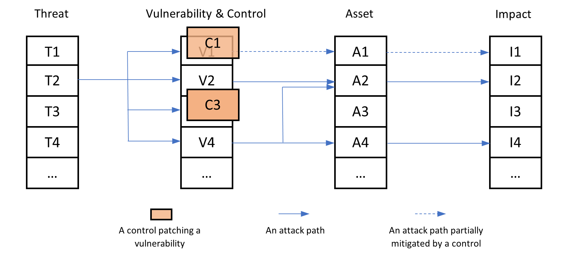
Figure 1: Cyber cascade model, and example of cyber incident, due to the second threat, where the first (resp. third) vulnerability is partially (resp. fully) patched by the first (resp. third) control

2.2 Mapping relationships among cascade components

To develop a quantitative cyber loss model based on the cascade model proposed by [7], this paper utilizes the relationships among the cascade components to define potential losses. As we can observe from Figure 1, since an asset being attacked induces one and only one impact, which shall be characterized by a random variable, there are only three mappings to be established, where the vulnerability serves as the core component and relates respectively to the threat, asset, and control. From now on, suppose that there are $l$ types of threats, $m$ categories of vulnerabilities, and $n$ classes of assets.

• Vulnerability-threat mapping

  This is a general many-to-many relationship, where a threat may exploit one or more vulnerabilities, and a vulnerability may be exploited by one or more threats. It characterizes the external risk by the intrinsic nature of a cyber event, which could be initiated externally or performed internally. This mapping is defined by a matrix $A$, which is of size $l\times m$, such that, for $i=1,2,\dots,l$ and $j=1,2,\dots,m$,

  $$A_{ij}=\begin{cases}1&\text{if {V}}j\text{ can be exploited by {T}}i;\\ 0&\text{otherwise.}\end{cases}$$

• Vulnerability-asset mapping

  This is another general many-to-many relationship, where a vulnerability may associate with one or more assets, and an asset may be associated with one or more vulnerabilities. It characterizes the internal risk by the overall configurations inside a cyber system. This mapping is defined by a matrix $B$ of size $m\times n$, such that, for $j=1,2,\dots,m$ and $k=1,2,\dots,n$,

  $$B_{jk}=\begin{cases}1&\text{if {A}$k$ is associated with {V}$j$};\\ 0&\text{otherwise}.\end{cases}$$

• Vulnerability-control mapping

  This is naturally a one-to-one and onto relationship based on the definition of controls. It characterizes the effectiveness of each control set in mitigating the corresponding vulnerability. For each vulnerability $j=1,2,\dots,m$, define $\theta_{j}\in\left[0,1\right]$ be the scaling factor to the potential loss(es) due to this V$j$, after a certain control set C$j$ is applied. When the vulnerability $j$ is only guarded by the control set at the industry standard, $\theta_{j}=1$. Note that the industry standard, instead of a completely insecure state that no control is applied at all, is considered in this paper, because many basic controls, such as built-in security features of many software applications, exist by default and thus an entirely insecure environment is nowhere to be found. Additional control measure C$j$ reduces the value of $\theta_{j}$; in particular, when the vulnerability $j$ is fully eliminated, $\theta_{j}=0$. The vulnerability-control mapping is summarized by the vector $\bm{\theta}=[\theta_{1},\theta_{2},\dots,\theta_{m}]$.

Since the vulnerabilities are shared across all three mappings, the relationships among threat, asset, and control can be obtained via composite mappings through the vulnerabilities. These mapping relationships indeed exist in practice, where cybersecurity controls are proposed to patch vulnerabilities and block pathways from threats to assets. For example, in the CIS (Center for Internet Security) Controls framework, [13] provided a comprehensive relationship between $20$ controls and $5$ assets; for illustration, the relationship is duplicated in Appendix A. Another example is that, based on this framework, [39] did an empirical study, which maps most of those CIS controls with $25$ threats compiled by [43]; the mapping is also repeated in Appendix B for demonstration.

Example 2.1.

To plainly illustrate the quantitative cyber loss model, we shall assume the following smaller mapping matrices to be referred repeatedly for risk assessment in the remaining of Section 2.

$$A=\bordermatrix{&\textsc{V1}&\textsc{V2}&\textsc{V3}\cr\textsc{T1}&0&1&0\cr\textsc{T2}&0&1&0\cr\textsc{T3}&0&1&1},\quad B=\bordermatrix{&\textsc{A1}&\textsc{A2}&\textsc{A3}\cr\textsc{V1}&1&0&1\cr\textsc{V2}&1&0&0\cr\textsc{V3}&1&1&0},\quad\bm{\theta}=\bordermatrix{&\textsc{V1}&\textsc{V2}&\textsc{V3}\cr&1/2&1/3&1/4}.$$

2.3 Tensor structure

With the aid of the three defined mappings above, we can define a single quantity for characterizing the effect by a cyber event on a controlled cyber system. To this end, for $i=1,2,\dots,l$, $j=1,2,\dots,m$, and $k=1,2,\dots,n$, let

$$D_{ijk}=A_{ij}B_{jk}\theta_{j}.$$ (1)

This quantity summarizes whether the cyber system is in danger of the cyber event, from the $i$-th threat by the $j$-th controlled vulnerability on the $k$-th asset, and if so, how extreme the impact is.

• If $D_{ijk}=1$, the $i$-th threat, $j$-th controlled vulnerability, and $k$-th asset together will induce full impact to the system. This is the aggregate result of that V$j$ is exploited by T$i$ and that A$k$ is associated with V$j$, and when no additional, other than industry standard, control C$j$ is implemented to patch V$j$.

• If $0<D_{ijk}<1$, the $i$-th threat, $j$-th controlled vulnerability, and $k$-th asset together will induce partial impact to the cyber system. Note that the partial impact here is defined relative to the full impact when $D_{ijk}=1$, and an impact is considered as partial when additional controls that exceed the industry-average level are implemented but are not yet able to completely eliminate the vulnerability. In this case, V$j$ is exploited by T$i$, A$k$ is associated with V$j$, and C$j$ only partially patches V$j$.

• If $D_{ijk}=0$, the $i$-th threat, $j$-th controlled vulnerability, and $k$-th asset together will not induce any impact to the system. This is either because, V$j$ cannot be exploited by T$i$, or A$k$ is not associated with V$j$, or V$j$ is fully patched by C$j$.

The structural information of the cyber cascade model can then be revealed in terms of a tensor $D$, of size $l\times m\times n$, which shall prove itself useful in developing the quantitative cyber loss model in later sections. To clearly picture this abstract object, we revisit Example 2.1 as follows.

Figure 2(a) depicts the tensor in Example 2.1, while Figure 2(b) summarizes the elements of that tensor. In the example, as there are $3$ types of threats, $3$ categories of vulnerabilities, and $3$ classes of assets, the tensor is defined in the finite set $\{\textsc{T}1,\textsc{T}2,\textsc{T}3\}\times\{\textsc{V}1,\textsc{V}2,\textsc{V}3\}\times\{\textsc{A}1,\textsc{A}2,\textsc{A}3\}$, where $\times$ represents the Cartesian product herein. The tensor can be generalized to include the three mappings by introducing the origin O; indeed, the vulnerability-threat matrix $A$ can be positioned on the $A$-plane, which is defined by the coordinates (T$i$, V$j$, O), while the vulnerability-asset matrix $B$ can be set on the $B$-plane, which is defined by the coordinates (O, V$j$, A$k$); the vulnerability-control vector $\bm{\theta}$ can be put on the $\bm{\theta}$-axis, which is defined by the coordinates (O, V$j$, O). Finally, the $O$-plane, which is defined by the coordinates (T$i$, O, A$k$) and represents the threat-asset mapping matrix $AB$, shall be handy in illustrating the cyber loss model in later sections. Such a generalization also applies for any finite set of threats, vulnerabilities, and assets.

(a) Tensor structure of cyber cascade model in Example 2.1

(b) Elements in tensor of Example 2.1

Figure 2: Example of tensor representation for cyber cascade model

2.4 Tensor-based cyber loss model

As pointed out in Section 2.1, an impact from each cyber incident is in fact a base random variable which models a random loss to the controlled cyber system. The impact depends on two factors. The first one is how the cyber event happens; that is, which threat is acted, either internally or externally, and in turn which vulnerability is exploited, as well as which asset is consequently affected; in addition, whether the vulnerability is patched. The first factor has been addressed by the tensor $D$ introduced in the last section, which depends on the controlled cyber system.

The second factor lies in the loss size itself. To this end, for $i=1,2,\dots,l$, $j=1,2,\dots,m$, and $k=1,2,\dots,n$, let $X_{ijk}^{0}$ be the random variable which represents the raw loss due to a cyber incident, from the $i$-th threat by the $j$-th vulnerability on the $k$-th asset. Herein, the raw loss represents a cyber loss which is not further mitigated by additional cybersecurity controls, but is mitigated by those at the industry-average level. These random variables can be summarized by another tensor $X^{0}$, of size $l\times m\times n$.

The contingent impact information from the cyber incident to the controlled cyber system of interest is then given by the element-wise product of the two tensors $D$ and $X^{0}$; that is,

$$X=D\circ X^{0},$$ (2)

where $\circ$ stands for the element-wise multiplication between two tensors herein. In particular, if the cyber incident is from the $i$-th threat, by the $j$-th controlled vulnerability, on the $k$-th asset, the impact will be given by $X_{ijk}=D_{ijk}X^{0}_{ijk}$; the impacts $X_{ijk}$ would practically be different among various threats, vulnerabilities, and assets.

The function of additional cybersecurity controls in this paper is to reduce the impacts from realized incidents, via the vector $\bm{\theta}$. One typical example of such an impact reduction is redundancy, such as database backups, which is not necessarily self-protecting cyber incidents from happening, but assures a speedy and inexpensive recovery. Reducing the probability, of future cyber incidents being emerged, by additional cybersecurity controls, similar to [34, 31, 48], shall be incorporated in future studies.

Example 2.2.

We revisit Example 2.1 to further illustrate the cyber loss model. While the structure of the tensor in Figure 3(a) of Example 2.1 is similar to that in Figure 2(a), they are actually different since Figure 3(a) depicts the loss tensor in which each element is an impact random variable, as shown in Figure 3(b). Therein, the elements are calculated based on Equation (2). For example, in accordance with Example 2.1, a viable attack path is represented by the red dashed arrows in Figure 3(a), where T$3$ is acted on V$3$, which is partially patched by C$3$, and consequently affects A$2$. The impact associated with that path is given by

$$X_{332}=D_{332}X^{0}_{332}=A_{33}B_{32}\theta_{3}X^{0}_{332}=\left(1/4\right)X^{0}_{332}.$$

However, if an attack path is not feasible, such as that T$3$ exploits V$3$ but A$3$ is not associated with V$3$, the impact will become null that

$$X_{333}=D_{333}X^{0}_{333}=A_{33}B_{33}\theta_{3}X^{0}_{333}=\left(0\right)X^{0}_{333}=0,$$

as $B_{33}=0$, even if the raw random loss $X^{0}_{333}$ is non-zero.

(a) Loss tensor and viable attack path in Example 2.1

(b) Elements in loss tensor of Example 2.1

Figure 3: Example of tensor-based cyber loss model

2.5 Aggregate cyber loss

The abstract tensor-based cyber loss model in the last section does not directly provide much practical use for enterprise risk management purposes. It is, instead, an aggregate cyber loss over a given time period, say one fiscal year, during which multiple cyber incidents might emerge (for example, a cyber attack might try several times to gain entry into a firm), would be called desirable to cyber risk managers. On one hand, as we shall see below, the loss model aggregating across cyber events is not new but based on the well-known collective risk model. On the other hand, the aggregate loss model for each cyber incident is derived by the loss tensor from the cascade model, which does not exist in the literature, and is based on, as alluded in Section 2.1, that a cyber event is due to a threat being acted.

2.5.1 Loss model for each cyber incident

We first fix a particular cyber event in the given period of time. Let $L$ be the aggregate loss of that cyber incident. Since each incident is initiated by one and only one threat, the aggregate loss is given by the sum of mutually exclusive losses, in which each loss is due to a unique threat. To this end, define, for $i=1,2,\dots,l$,

$$Y_{i}=\begin{cases}1&\text{if T}i\text{ is attempted};\\ 0&\text{otherwise},\end{cases}$$

where, for any distinct $i_{1},i_{2}=1,2,\dots,l$, $\mathbb{P}\left(Y_{i_{1}}=1,Y_{i_{2}}=1\right)=0$ and $\sum_{i=1}^{l}\mathbb{P}\left(Y_{i}=1\right)=1$; denote $\mathbb{P}\left(Y_{i}=1\right)$ by $p_{i}$, and thus $\sum_{i=1}^{l}p_{i}=1$. Moreover, let $Z_{i}$ be the random loss due to the $i$-th threat, for $i=1,2,\dots,l$; since each threat exploits multiple controlled vulnerabilities, while each vulnerability associates with multiple assets, several impacts would be materialized due to that particular threat being acted; consequently,

$$Z_{i}=\sum_{k=1}^{n}\sum_{j=1}^{m}X_{ijk}=\sum_{j=1}^{m}X_{ij1}+\sum_{j=1}^{m}X_{ij2}+\dots+\sum_{j=1}^{m}X_{ijn}.$$

While the order of the double summations does not matter, we choose to aggregate the impacts across vulnerabilities first, and then across assets, to prepare for cyber capital management in later sections, where we shall provide practical reasons for this order. Let also $Z_{ik}$ be the random loss due to the $i$-th threat on the $k$-th asset, for $i=1,2,\dots,l$ and $k=1,2,\dots,n$; and thus,

$$Z_{ik}=\sum_{j=1}^{m}X_{ijk}\quad\text{and}\quad Z_{i}=\sum_{k=1}^{n}Z_{ik}.$$ (3)

Therefore, the aggregate loss of the cyber event is given by

$$L=\sum_{i=1}^{l}Z_{i}\mathds{1}_{\left\{Y_{i}=1\right\}}.$$ (4)

Revisiting Example 2.1 should ease the understanding of this series of aggregations. Figure 4 illustrates that the impact aggregation across vulnerabilities in (3) can be pictorially understood as compressing the impact random variables in the loss tensor towards the $O$-plane. Moreover, from Figure 4, the additional impact aggregation across assets in (3) can be realized as further compressing the aggregated random losses on the $O$-plane towards the T$i$-axis. Finally, the materialized aggregate loss in (4) due to the cyber incident picks either $Z_{1}$, $Z_{2}$, or $Z_{3}$ on the T$i$-axis.

Figure 4: Impact aggregation across vulnerabilities and assets in Example 2.1

By (3) and (4), the distribution of aggregate loss of the cyber incident can be obtained by two convolutions, followed by a mixing:

$$f_{Z_{ik}}=f_{X_{i1k}}\ast f_{X_{i2k}}\ast\dots\ast f_{X_{imk}},\quad\text{for $i=1,2,\dots,l$ and $k=1,2,\dots,n$};$$ (5)

$$f_{Z_{i}}=f_{Z_{i1}}\ast f_{Z_{i2}}\ast\dots\ast f_{Z_{in}},\quad\text{for $i=1,2,\dots,l$};\quad f_{L}=\sum_{i=1}^{l}p_{i}f_{Z_{i}},$$ (6)

where $\ast$ represents the convolution operator, and $f_{R}$ is the probability density function of a generic random variable $R$.

2.5.2 Collective risk model

Armed with the aggregate loss model for each cyber event, the aggregate loss model over the given period of time is simply resembling the renowned collective risk model. Let $N$ be a non-negative random variable that represents the total number of cyber incidents. Let $L^{r}$, for $r=1,2,\dots$, be a sequence of independent and identically distributed aggregate losses, where $L^{r}$ represents the aggregate loss of the $r$-th cyber incident and follows the distribution of $f_{L}$ given in (6). Assume that the total number of cyber incidents $N$ is independent of the aggregate losses $L^{r}$. Therefore, the total aggregate loss over the given time period $S=\sum_{r=1}^{N}L^{r}$, and its probability density function is given by

$$f_{S}=\lim_{\tilde{n}\rightarrow\infty}\sum_{r=0}^{\tilde{n}}\left(f_{L^{1}}\ast f_{L^{2}}\ast\dots\ast f_{L^{r}}\right)\times p_{N}\left(r\right),$$ (7)

where $p_{N}\left(\cdot\right)$ is the probability mass function of the random variable $N$.

For the purpose of cyber capital management in later sections, let $S_{ik}$ be the aggregate loss of cyber incidents from the $i$-th threat on the $k$-th asset over the given time period, where $i=1,2,\dots,l$ and $k=1,2,\dots,n$. It can be expressed as $S_{ik}=\sum_{r=1}^{N_{ik}}Z_{ik}^{r}$, where $N_{ik}$ is a non-negative random variable to represent the number of cyber incidents from the $i$-th threat on the $k$-th asset, and $Z_{ik}^{r}$, for $r=1,2,\dots$, is a sequence of independent and identically distributed random losses due to T$i$ on A$k$, and each $Z_{ik}^{r}$ represents the random loss of the $r$-th cyber incident associated with (T$i$,A$k$) and follows the distribution of $f_{Z_{ik}}$ given in (5). The distribution of $S_{ik}$ can be obtained in a similar manner as in (7), as long as $N_{ik}$ and $Z_{ik}^{r}$ are independent. Note that $S=\sum_{i=1}^{l}\sum_{k=1}^{n}S_{ik}$. We, again, defer providing the practical reasons for this choice of granularity for aggregate loss to the next section.

Recall also that this paper considers additional cybersecurity controls, modeled by the vector $\bm{\theta}$, on only reducing the impacts from the incidents but not on reducing the likelihood of a cyber incident. If the latter case were incorporated, the random variables $N$ and $N_{ik}$, for $i=1,2,\dots,l$ and $k=1,2,\dots,n$, would have been depending on another risk mitigation vector.

3 Cyber Capital Management

As in general risk management practice, company managers can make use of the quantitative loss model developed in the previous section to outline capital allocation schemes for cyber risks. Such schemes should consist of three sequential components: risk reduction, transfer, and retention. For risk reduction, ex-ante investment should be budgeted to improve the existing cybersecurity controls or implement new ones to reduce potential cyber losses. For risk transfer, cyber insurance coverage should then be purchased by paying a premium to further reduce the exposure. For risk retention, ex-post-loss reserve should be planned to weather the potential residual cyber losses and to ensure uninterrupted business operations.

Existing literature focuses on only one or two of the aforementioned components, but to align well with enterprise risk management principles, a comprehensive and holistic approach to these components should be developed. This section first discusses the roles and interactions of the corresponding capitals for cyber risk reduction, transfer, and retention. It then presents a novel capital allocation model for designing the budgeting decisions on cybersecurity investment, cyber insurance, and reserve based on the proposed cyber risk assessment model in the previous section.

3.1 Trade-off: ex-ante versus ex-post-loss capitals

Recall that the cyber cascade model is characterized by the three mappings defined in Section 2.2. The vulnerability-threat and vulnerability-asset mappings are typically determined by the company’s cyber infrastructure and external factors of cyber actions. Company managers have the authority to allocate ex-ante capital for cybersecurity investments to revise the vulnerability-control mapping. Therefore, an impact, i.e., a loss, from each cyber incident can be reduced through partially, or even fully, patching the currently existing vulnerabilities, i.e., any remaining vulnerabilities after industry-standard controls have already been applied, via investment in additional cybersecurity controls.

Let $M_{j}$, for $j=1,2,\dots,m$, be the cybersecurity investment amount to the control C$j$ for the vulnerability V$j$. The investment amount $M_{j}$ to the $j$-th control, in turn, affects the scaling factor to the potential loss(es) due to the V$j$, which is $\theta_{j}\left(M_{j}\right)$; in particular, the investment amount and the scaling factor are inversely proportional to each other, that when the ex-ante investment is large, the scaling factor becomes small, and vice versa. Since the total aggregate loss $S$, and the aggregate loss $S_{ik}$ because of (T$i$,A$k$), for $i=1,2,\dots,l$ and $k=1,2,\dots,n$, over the given period of time, depend on the scaling vector $\bm{\theta}$, they are actually driven by the investment vector $\mathbf{M}=\left[M_{1},M_{2},\dots,M_{m}\right]$. In the sequel, we shall write such dependence for the aggregate losses $S_{ik}\left(\mathbf{M}\right)$.

They guide us to the underlying trade-off between ex-ante capital, which is the cybersecurity investment, and ex-post-loss capitals, which include the premium for cyber insurance coverage, and the reserve. When the management allocates no or little additional capital for the cybersecurity investment beyond the industry standard, the scaling factor vanishes such that the cyber system experiences almost full impact from contingent cyber events. In this case, the realized aggregate losses within the period could be massive, which requires the management to plan a tremendous amount of, premium for a sufficient insurance coverage to transfer, and reserve to absorb losses. For example, in the 2017 WannaCry attack, where the threat was encrypting ransomware, many organizations were exposed to it because of their lack of data recovery capability, which is the exploited vulnerability in such events. However, this vulnerability could have been easily patched by relatively low cost measures such as reliable backups for important data, and thus the materialized impact of the attack could have been substantially reduced, which leads to a lower cost of business or production recovery from data inaccessibility. This corresponds to the left side of the curve in Figure 5, where a marginal increase in cybersecurity investment can significantly reduce the expected amount of spending on recovery after cyber incidents and reduce the total allocated capital.

However, this does not necessarily imply that the cyber risk manager should fully allocate ex-ante capital for cybersecurity investment only. The well-known Gordon-Loeb model (see [24, 26]) states that the marginal benefit, in terms of the expected loss reduction, decreases for each unit of cybersecurity investment. Therefore, as pointed out by [38], if the total allocated capital is to be minimized, there will be a certain level of cybersecurity investment such that any additional ex-ante capital allocation is not worthy of such a small marginal return. This corresponds to the right side of the curve in Figure 5.

Overall, the shape of the curve in Figure 5 resembles the Laffer curve in economics. Both curves reveal that the present cost could have an effect on the resulting costs for the future; moreover, due to the diminishing marginal benefit of the present cost, a right balance between the two costs could be determined.

Figure 5: Trade-off between ex-ante and ex-post-loss capitals for cyber risks

3.2 Optimal capital allocation

Finding such sweet spot for the ex-ante and ex-post-loss capitals trade-off should be one of the key elements to be considered in any cyber capital management practice. Regarding the investment decision, there is no ambiguity that they should be for cybersecurity controls that patch vulnerabilities. However, the company could buy insurance coverage and keep reserves for different classes of targets. For example, the company could set aside funds for individual assets, e.g., separate reserves for data and physical assets. Similarly, insurance coverage could be purchased specifically for different threats. In this paper, we follow some existing practices in the cybersecurity and cyber insurance industries. For instance, the CyberOne^TM Coverage offered by [27] covers cyber losses resulting from different attacks, such as malware and denial-of-service attacks, which are various types of threats; see also [12] for incident-specific cyber insurance. The covered losses in the CyberOne^TM Coverage include data and system restoration costs, which arise from various classes of assets. As another example, cyber risk management tools and services, such as the Thrivaca model by [3], offer their clients the estimation of cyber losses at the granularity of threat-asset pairs. Therefore, the insurance coverage is written on the aggregate loss $S_{ik}\left(\mathbf{M}\right)$ due to (T$i$,A$k$), for $i=1,2,\dots,l$, and $k=1,2,\dots,n$, while the reserve is allocated to any retained part of this aggregate loss. This echoes the choice of granularity for aggregate loss in Section 2.

In addition, there are three other common conflicting interests and priorities in a general capital management framework, which we review as follows and shall provide a detailed account after formulating the optimal capital allocation problem.

• (Standalone and corporate allocations) Naturally, the management has to budget total capital at the whole corporate level which concerns the aggregate loss. For project financing, performance measure, and regulatory supervision purposes, the management also has to allocate capital at standalone levels.

• (Loss-reserve matching and reduction in opportunity cost) On the one hand, the cyber risk manager should plan and allocate reserves at corporate and standalone levels which do not deviate much from the realized retained aggregate losses. On the other hand, reserve needs to be kept as liquid assets, such as cash and money market funds, which typically yield little return; the liquidity requirement causes an opportunity cost, which should be minimized.

• (Ex-post-loss premium and reserve allocations) There is an additional layer of trade-off between the two ex-post-loss capitals. If the cyber risk manager is willing to pay a higher premium to transfer a larger part of the aggregate loss to the insurer, a smaller portion of the loss will be retained, which in turn reduces the needed reserve.

In order to achieve these three compromises altogether, we propose to apply the holistic principle by [11], which allows the manager to solve the cyber capital allocation as one single optimization problem; see also its recent application to pandemic resources management in [10].

$$\inf_{\begin{subarray}{c}\mathbf{M},{\mathbf{I},}\mathbf{K}\in\mathcal{A}\end{subarray}} \;\underbrace{\sum_{j=1}^{m}\eta_{j}M_{j}}_{\leavevmode\hbox to8.9pt{\vbox to8.9pt{\text{[drawing]}}}}{+\underbrace{\sum_{i=1}^{l}\sum_{k=1}^{n}\alpha_{ik}\Pi\left[I_{ik}(S_{ik}(\mathbf{M}))\right]}_{\leavevmode\hbox to8.9pt{\vbox to8.9pt{\text{[drawing]}}}}}+\underbrace{\sum_{i=1}^{l}\sum_{k=1}^{n}\nu_{ik}K_{ik}}_{\leavevmode\hbox to8.9pt{\vbox to8.9pt{\text{[drawing]}}}}$$ (8)

$$\;+\underbrace{\sum_{i=1}^{l}\sum_{k=1}^{n}\omega_{ik}\mathbb{E}\left[\left({R_{ik}(S_{ik}(\mathbf{M}))}-K_{ik}\right)^{2}h_{ik}\left({R_{ik}(S_{ik}(\mathbf{M}))}\right)\right]}_{\leavevmode\hbox to8.9pt{\vbox to8.9pt{\text{[drawing]}}}}$$

$$\;+\underbrace{\eta M}_{\leavevmode\hbox to8.9pt{\vbox to8.9pt{\text{[drawing]}}}}{+\underbrace{\alpha\sum_{i=1}^{l}\sum_{k=1}^{n}\Pi\left[I_{ik}(S_{ik}(\mathbf{M}))\right]}_{\leavevmode\hbox to8.9pt{\vbox to8.9pt{\text{[drawing]}}}}}+\underbrace{\nu K}_{\leavevmode\hbox to8.9pt{\vbox to8.9pt{\text{[drawing]}}}}$$

$$\;+\underbrace{\omega\mathbb{E}\left[\left({\sum_{i=1}^{l}\sum_{k=1}^{n}R_{ik}(S_{ik}(\mathbf{M}))}-K\right)^{2}h\left({\sum_{i=1}^{l}\sum_{k=1}^{n}R_{ik}(S_{ik}(\mathbf{M}))}\right)\right]}_{\leavevmode\hbox to8.9pt{\vbox to8.9pt{\text{[drawing]}}}},$$

where

• $\mathcal{A}=\mathcal{M}\times{\mathscr{F}\times}\mathcal{K}\subseteq\mathbb{R}^{m}\times{\mathcal{I}\times}\mathbb{R}^{l\times n}$. $\mathcal{M}$ is the set of admissible ex-ante cybersecurity investment allocation $\mathbf{M}=\left[M_{1},M_{2},\dots,M_{m}\right]$, and $M=\sum_{j=1}^{m}M_{j}$ is the corporate investment; $\mathcal{K}$ is the set of admissible ex-post-loss reserve allocation $\mathbf{K}=\left[K_{ik}\right]_{i=1,2,\dots,l;k=1,2,\dots,n}$, and $K=\sum_{i=1}^{l}\sum_{k=1}^{n}K_{ik}$ is the corporate reserve; $\mathcal{I}$ is the set of admissible indemnity functions $\mathbf{I}=\left[I_{ik}(\cdot)\right]_{i=1,2,\dots,l;k=1,2,\dots,n}$ for aggregate losses on threat-asset pairs, which shall be defined next, while $\mathscr{F}$ is a subset of $\mathcal{I}$;

• $R_{ik}(\cdot)$ and $I_{ik}(\cdot)$ are respectively the so-called retained and indemnity functions for the aggregate loss $S_{ik}$ on the threat-asset pair (T$i$,A$k$), for $i=1,2,\dots,l$, and $k=1,2,\dots,n$. Note that $R_{ik}(\cdot)+I_{ik}(\cdot)=\mathrm{Id}(\cdot)$, where $\mathrm{Id}(\cdot)$ is the identity function; that is, for a realized loss $s_{ik}(\mathbf{M})$, $R_{ik}(s_{ik}(\mathbf{M}))$ is absorbed by the company, and the other part $I_{ik}(s_{ik}(\mathbf{M}))$ is transferred to the insurer. The admissible set $\mathcal{I}$ of indemnity functions is defined as

  $$\mathcal{I}=\{\left[I_{ik}(\cdot)\right]_{i=1,2,\dots,l;k=1,2,\dots,n}:0\leq I_{ik}(\cdot)\leq\mathrm{Id}(\cdot);\;I_{ik}(\cdot)\text{ and }R_{ik}(\cdot)\text{ are non-decreasing}\},$$

  to ensure that the insurance coverage for each aggregate loss $S_{ik}$ satisfies the principle of indemnity and does not lead to any ex-post moral hazards. The functional $\Pi\left(\cdot\right)$ denotes a general premium principle, and thus represents the weighted standalone premiums, in plain dollar unit, paid for coverage to individual threat-asset pairs, and is the total premium, in plain dollar unit, weighted at the corporate level. In the sequel, to simplify the notations, we shall write $I_{ik}(\mathbf{M})$ and $R_{ik}(\mathbf{M})$, for $I_{ik}(S_{ik}(\mathbf{M}))$ and $R_{ik}(S_{ik}(\mathbf{M}))$, as well as $I(\mathbf{M})$ and $R(\mathbf{M})$, for $\sum_{i=1}^{l}\sum_{k=1}^{n}I_{ik}(S_{ik}(\mathbf{M}))$ and $\sum_{i=1}^{l}\sum_{k=1}^{n}R_{ik}(S_{ik}(\mathbf{M}))$, while $\pi_{ik}(\mathbf{M},I_{ik})$ and $\pi(\mathbf{M},\mathbf{I})$, for $\Pi\left[I_{ik}(S_{ik}(\mathbf{M}))\right]$ and $\sum_{i=1}^{l}\sum_{k=1}^{n}\Pi\left[I_{ik}(S_{ik}(\mathbf{M}))\right]$;

• $\eta_{j},{\alpha_{ik},}\nu_{ik},\omega_{ik},\eta,{\alpha,}\nu,\omega\geq 0$ are the weights of objectives. Notice that, since the weighted expected deviances, $\mathbb{E}\left[\left({R_{ik}(\mathbf{M})}-K_{ik}\right)^{2}h_{ik}\left({R_{ik}(\mathbf{M})}\right)\right]$ and $\mathbb{E}\left[\left({R(\mathbf{M})}-K\right)^{2}h\left({R(\mathbf{M})}\right)\right]$, are quadratic, their units are measured in square dollars; yet, as the opportunity cost of allocated capitals, $M_{j}$, $K_{ik}$, $M$, and $K$, are linear, their units are measured in plain dollar; recall also that (total) premiums are also measured in plain dollar units. To practically and fairly consider their aggregate effects as in (8), the weights of the expected deviances, $\omega_{ik}$ and $\omega$, are composed of importance weights with no dollar unit, $\omega_{ik}^{\text{I}}$ and $\omega^{\text{I}}$, and unit-exchange weights with reciprocal dollar units, $\omega_{ik}^{\text{E}}$ and $\omega^{\text{E}}$, that each weight is their products, i.e., $\omega_{ik}=\omega_{ik}^{\text{I}}\omega_{ik}^{\text{E}}$ for $i=1,2,\dots,l$ and $k=1,2,\dots,n$, and $\omega=\omega^{\text{I}}\omega^{\text{E}}$. The importance weights, $\omega_{ik}^{\text{I}}$ and $\omega^{\text{I}}$, are compared relatively with other importance weights of no dollar unit, $\eta_{j}$, $\alpha_{ik}$, $\nu_{ik}$, $\eta$, $\alpha$, and $\nu$. The choice of unit-exchange weights, $\omega_{ik}^{\text{E}}$ and $\omega^{\text{E}}$, shall be discussed with an aid of the numerical example in Section 4;

• $h_{ik}\left({\cdot}\right)$ and $h\left({\cdot}\right)$ are the weighted penalty functions, for which $\mathbb{E}\left[h_{ik}\left(S_{ik}\right)\right]=\mathbb{E}\left[h\left(S\right)\right]=1$, which measure the deviation of realized retained aggregate losses from the allocated reserve intended to cover the losses; the family of such functions is summarized in [23, 15, 11].

The holistic cyber capital allocation solved by (8) shall indeed take those three equilibriums into account, which can also be read from various pieces in the objective function.

• (Standalone and corporate allocations) The standalone allocation scheme is represented by , , , and , where investments on cybersecurity controls, transferred losses, and reserves are balanced on the level of vulnerabilities and threat-asset pairs. In contrast, , , , and together represent the corporate allocation scheme, in which the total investment, insured loss, and reserve are determined in the equilibrium.

• (Loss-reserve matching and reduction in opportunity cost) The matchings are given in for standalone allocations, and in for corporate allocation. They are achieved by minimizing the mismatching cost, which is the weighted expected deviance between the realized retained aggregate loss and the allocated reserve for covering the loss. The deviance is given in the quadratic form since cyber incidents might cause ripple effects, as described in [42], which could lead to additional losses if the initial impact cannot be well contained due to the lack of reserve. Therefore, the relationship between loss-reserve mismatching and its cost should be non-linear. For instance, if a cyber attack disrupts the production lines of a manufacturer, and there is not sufficient fund nor insurance coverage for resuming the operation promptly, the manufacturer may face additional contractual liabilities for the late delivery of products. As for minimizing the opportunity cost for holding liquid assets as reserve, they are represented by for standalone allocations, and by for corporate allocation.

• (Ex-post-loss premium and reserve allocations) The cost of standalone premiums is given by their weighted sum , while the counterpart in the corporate level is given by . The trade-off between the two ex-post-loss capitals, which are the premium and reserve, discussed in Section 3.2 can be revealed in (8). Should the insurance coverage be larger, the retained aggregate losses of the company are reduced, and thus, by and , the needed reserves matching for the losses, as well as their opportunity costs given in and , are also lowered; yet, the insurer should charge more for the premium, and hence the cost of premiums are increased in and .

• (Ex-ante and ex-post-loss capitals) The trade-off between ex-ante and ex-post-loss capitals introduced in Section 3.1 is also weighed in. The costs of cybersecurity investment are given in for standalone allocations, and in for corporate allocation, whereas the standalone and corporate insurance coverage and reserve costs are , , and together, as well as , , and together, respectively. Note that the cost of reserve incorporates the consideration for the balancing between sufficient loss reserve and economical opportunity cost, as discussed in the second point above.

3.3 Holistic cyber capital allocation

The capital allocation problem in (8) can be solved in two steps. First, for each cybersecurity investment $\mathbf{M}\in\mathcal{M}$ and for each combination of indemnity functions $\mathbf{I}\in\mathscr{F}$, the optimal ex-post-loss reserve allocation $\mathbf{K}^{*}\in\mathcal{K}$, which depends on the fixed investment $\mathbf{M}$ and indemnity functions $\mathbf{I}$, is solved from (8) without the objective terms , , , and . Then, the optimal reserve $\mathbf{K}^{*}\left(\mathbf{M},\mathbf{I}\right)$ is substituted back into (8), which is solved for the optimal investment $\mathbf{M}^{*}$ and optimal indemnities $\mathbf{I}^{*}$. Consequently, the optimal cybersecurity investment, insurance coverage, and reserve allocation are given by the tuple $\left(\mathbf{M}^{*},\mathbf{I}^{*},\mathbf{K}^{*}\left(\mathbf{M}^{*},\mathbf{I}^{*}\right)\right)$. The first step was partially resolved in [11], while we shall herein impose an additional total budget constraint for cybersecurity investments, premiums, and reserves together. As pointed out in [40], most organizations do not have the fund to implement strong security, and thus cyber risk management decisions can only be made with a limited budget in most cases. For the optimal investment $\mathbf{M}^{*}$ and insurance $\mathbf{I}^{*}$ in the second step, a pairwise comparison between admissible investment allocations, and between admissible insurance coverages, shall again shed light on the trade-offs, between ex-post-loss premium and reserve allocations, and between ex-ante and ex-post-loss capitals. In the sequel, an investment or a reserve is admissible as long as it is non-negative, which should be practically assumed.

3.3.1 Optimal ex-post-loss reserve

Throughout this subsection, fix a non-negative investment allocation $\mathbf{M}$ and admissible indemnities $\mathbf{I}$, such that $M{+\pi(\mathbf{M},\mathbf{I})}\leq\beta$, where $\beta$ is the total budget for cybersecurity investment, premium for insurance, and reserve allocations.

We shall first present the unconstrained solution, i.e., when $\mathcal{K}=\mathbb{R}^{l\times n}$ in (8), as it shall lead us on how to solve the optimal reserve with constraints. In this paper, two sets of constraints shall be considered for practicality. We first show how reserves should be determined if they are only subject to the non-negativity requirement, and then, in addition, a total budget constraint is assumed.

Unconstrained case

With $\mathcal{K}=\mathbb{R}^{l\times n}$, the optimal ex-post-loss reserve $\widetilde{\mathbf{K}}^{*}\left(\mathbf{M},\mathbf{I}\right)$ is given by, for any $i^{\prime}=1,2,\dots,l$, and $k^{\prime}=1,2,\dots,n$,

$${\widetilde{K}^{*}_{i^{\prime}k^{\prime}}\left(\mathbf{M},\mathbf{I}\right)}={\overline{K}_{i^{\prime}k^{\prime}}\left(\mathbf{M},\mathbf{I}\right)}-\widetilde{W}_{i^{\prime}k^{\prime}}\left(\sum_{i=1}^{l}\sum_{k=1}^{n}{\overline{K}_{ik}\left(\mathbf{M},\mathbf{I}\right)}-{\overline{K}\left(\mathbf{M},\mathbf{I}\right)}\right),$$ (9)

and the corporate reserve is

$${\widetilde{K}^{*}\left(\mathbf{M},\mathbf{I}\right)}=\sum_{i=1}^{l}\sum_{k=1}^{n}{\widetilde{K}^{*}_{ik}\left(\mathbf{M},\mathbf{I}\right)}={\overline{K}\left(\mathbf{M},\mathbf{I}\right)}+\widetilde{W}\left(\sum_{i=1}^{l}\sum_{k=1}^{n}{\overline{K}_{ik}\left(\mathbf{M},\mathbf{I}\right)}-{\overline{K}\left(\mathbf{M},\mathbf{I}\right)}\right),$$

where, for any $i^{\prime}=1,2,\dots,l$, and $k^{\prime}=1,2,\dots,n$,

$${\overline{K}_{i^{\prime}k^{\prime}}\left(\mathbf{M},\mathbf{I}\right)}=\mathbb{E}\left[{R_{i^{\prime}k^{\prime}}(\mathbf{M})}h_{i^{\prime}k^{\prime}}\left({R_{i^{\prime}k^{\prime}}(\mathbf{M})}\right)\right]-\frac{\nu_{i^{\prime}k^{\prime}}}{2\omega_{i^{\prime}k^{\prime}}},\quad{\overline{K}\left(\mathbf{M},\mathbf{I}\right)}=\mathbb{E}\left[{R(\mathbf{M})}h\left({R(\mathbf{M})}\right)\right]-\frac{\nu}{2\omega},$$ (10)

$$\widetilde{W}_{i^{\prime}k^{\prime}}=\frac{\frac{1}{\omega_{i^{\prime}k^{\prime}}}}{\frac{1}{\omega}+\sum_{i=1}^{l}\sum_{k=1}^{n}\frac{1}{\omega_{ik}}},\quad\widetilde{W}=\frac{\frac{1}{\omega}}{\frac{1}{\omega}+\sum_{i=1}^{l}\sum_{k=1}^{n}\frac{1}{\omega_{ik}}};$$

for its proof, see [11]. These four components constituting the optimal and corporate reserves are respectively the optimal standalone reserve $\overline{K}_{i^{\prime}k^{\prime}}\left(\mathbf{M},\mathbf{I}\right)$, the optimal corporate reserve $\overline{K}\left(\mathbf{M},\mathbf{I}\right)$, and harmonic weights $\widetilde{W}_{i^{\prime}k^{\prime}}$, $\widetilde{W}$. Note that $\widetilde{W}+\sum_{i=1}^{l}\sum_{k=1}^{n}\widetilde{W}_{ik}=1$. The optimal standalone reserve describes the amount planned for a particular threat-asset pair $\left(\text{T}i^{\prime},\text{A}k^{\prime}\right)$ if it were the only pair to be allocated with reserve. When $\nu_{i^{\prime}k^{\prime}}$ is relatively larger than $\omega_{i^{\prime}k^{\prime}}$, i.e., it is more costly to allocate reserve for the threat-asset pair $\left(\text{T}i^{\prime},\text{A}k^{\prime}\right)$, in terms of the opportunity cost over the loss-reserve mismatching cost, its optimal reserve is reduced. Similar interpretations hold for the optimal corporate reserve. The harmonic weights represent the competition among optimal standalone reserves and the optimal corporate reserve. When $\omega_{i^{\prime}k^{\prime}}$ is relatively larger than the other $\omega_{ik}$ and $\omega$, the corresponding harmonic weight $\widetilde{W}_{i^{\prime}k^{\prime}}$ is small, and thus the optimal reserve inclines to its own optimal standalone reserve.

Constrained case: non-negative reserves

Let us discuss the case when the non-negativity constraint, i.e., $\mathcal{K}=\mathbb{R}^{l\times n}_{+}$, is imposed. On the one hand, if all of the unconstrained optimal ex-post-loss reserves solved in (9) satisfy the constraint, they are also optimal for the constrained case. On the other hand, if some of the unconstrained reserves solved in (9) do not satisfy the constraint, they should instead be assigned by the lower bound of a reserve, which is zero in this setting. Hence, these threat-asset pairs should not compete with other pairs, as well as the whole corporate, for reserve resources, and this should be reflected in the revised harmonic weights, which exclude those non-competing threat-asset pairs. However, before all of the constrained optimal ex-post-loss reserves are solved, the exact threat-asset pairs being bound by the non-negativity constraint are not known a priori. To this end, we introduce an auxiliary variable $\delta_{ik}$, for $i=1,2,\dots,l$, and $k=1,2,\dots,n$, which takes a value either $0$ or $1$. Then, all of the constrained optimal ex-post-loss reserves $K^{+}_{i^{\prime}k^{\prime}}\left(\mathbf{M},\mathbf{I}\right)$, together with the auxiliary variables as by-products, are solved by the following set of equations.

$${K^{+}_{i^{\prime}k^{\prime}}\left(\mathbf{M},\mathbf{I}\right)}=\begin{cases}{K_{i^{\prime}k^{\prime}}\left(\mathbf{M},\mathbf{I}\right)}&\text{if}\quad{K_{i^{\prime}k^{\prime}}\left(\mathbf{M},\mathbf{I}\right)}\geq 0\\ 0&\text{if}\quad{K_{i^{\prime}k^{\prime}}\left(\mathbf{M},\mathbf{I}\right)}<0\end{cases},\quad\mathds{1}_{\left\{{K_{i^{\prime}k^{\prime}}\left(\mathbf{M},\mathbf{I}\right)}\geq 0\right\}}={\delta_{i^{\prime}k^{\prime}}},$$ (11)

for all $i^{\prime}=1,2,\dots,l$, and $k^{\prime}=1,2,\dots,n$, where

$${K_{i^{\prime}k^{\prime}}\left(\mathbf{M},\mathbf{I}\right)}={\overline{K}_{i^{\prime}k^{\prime}}\left(\mathbf{M},\mathbf{I}\right)}-W_{i^{\prime}k^{\prime}}^{+}\left(\sum_{i=1,i\neq i^{\prime}}^{l}\sum_{k=1,k\neq k^{\prime}}^{n}{\overline{K}_{ik}\left(\mathbf{M},\mathbf{I}\right)\delta_{ik}}+{\overline{K}_{i^{\prime}k^{\prime}}\left(\mathbf{M},\mathbf{I}\right)}-{\overline{K}\left(\mathbf{M},\mathbf{I}\right)}\right),$$

and the optimal standalone reserve $\overline{K}_{i^{\prime}k^{\prime}}\left(\mathbf{M},\mathbf{I}\right)$, as well as the optimal corporate reserve $\overline{K}\left(\mathbf{M},\mathbf{I}\right)$, are still given by (10), but the harmonic weight is revised as

$$W_{i^{\prime}k^{\prime}}^{+}=\frac{\frac{1}{\omega_{i^{\prime}k^{\prime}}}}{\frac{1}{\omega}+\frac{1}{\omega_{i^{\prime}k^{\prime}}}+\sum_{i=1,i\neq i^{\prime}}^{l}\sum_{k=1,k\neq k^{\prime}}^{n}\frac{1}{\omega_{ik}}{\delta_{ik}}}.$$

For a further detailed account of the constrained solution and the proof of obtaining the set of equations, see [11].

Constrained case: non-negative reserves with total budget

For many businesses, there could only be a limited amount of capital devoted to cyber risk management, which may not be sufficient to meet the reserving scheme given by Equation (11). Since $\beta\geq 0$ is the total budget for cybersecurity investment, premium for insurance, and reserve allocations, for the fixed investment allocation $\mathbf{M}$ and insurance coverages $\mathbf{I}$, the remaining budget for ex-post-loss reserves is ${b\left(\mathbf{M},\mathbf{I}\right)}:=\beta-M{-\pi(\mathbf{M},\mathbf{I})}$. Together with the non-negative reserve constraint, $\mathcal{K}=\mathbb{R}^{l\times n}_{+}\cap\left\{{\mathbf{K}(\mathbf{M},\mathbf{I})}\;\middle|\;\sum_{i=1}^{l}\sum_{k=1}^{n}{K_{ik}(\mathbf{M},\mathbf{I})}\leq{b\left(\mathbf{M},\mathbf{I}\right)}\right\}$.

Let $K_{i^{\prime}k^{\prime}}^{*}\left(\mathbf{M},\mathbf{I}\right)$, for $i^{\prime}=1,2,\dots,l$ and $k^{\prime}=1,2,\dots,n$, be the solution in this scenario. The total budget constraint is not binding if $\sum_{i=1}^{l}\sum_{k=1}^{n}{K^{+}_{ik}(\mathbf{M},\mathbf{I})}\leq{b\left(\mathbf{M},\mathbf{I}\right)}$, which essentially results in the solution given by Equation (11), i.e., $K_{i^{\prime}k^{\prime}}^{*}\left(\mathbf{M},\mathbf{I}\right)=K_{i^{\prime}k^{\prime}}^{+}\left(\mathbf{M},\mathbf{I}\right)$. Therefore, we shall only consider the case in which the total budget for reserves is smaller than $\sum_{i=1}^{l}\sum_{k=1}^{n}{K^{+}_{ik}(\mathbf{M},\mathbf{I})}$.

By the Karush–Kuhn–Tucker conditions, the optimal ex-post-loss reserves under the binding budget constraint, $K_{i^{\prime}k^{\prime}}^{*}\left(\mathbf{M},\mathbf{I}\right)$, can be expressed as follows,

$${K^{*}_{i^{\prime}k^{\prime}}\left(\mathbf{M},\mathbf{I}\right)}=\begin{cases}{\overline{K}_{i^{\prime}k^{\prime}}\left(\mathbf{M},\mathbf{I}\right)}-W_{i^{\prime}k^{\prime}}\left(\sum_{(i,k)\in{\mathfrak{I}}}{\overline{K}_{ik}\left(\mathbf{M},\mathbf{I}\right)}-{b\left(\mathbf{M},\mathbf{I}\right)}\right)&\text{if}\quad(i^{\prime},k^{\prime})\in{\mathfrak{I}}\\ 0&\text{if}\quad(i^{\prime},k^{\prime})\notin{\mathfrak{I}}\end{cases},$$ (12)

where $W_{i^{\prime}k^{\prime}}$ is the harmonic weight given by $W_{i^{\prime}k^{\prime}}=\frac{1}{\omega_{i^{\prime}k^{\prime}}}/\sum_{(i,k)\in{\mathfrak{I}}}\frac{1}{\omega_{ik}}$, and the set of indices $\mathfrak{I}$ is a subset of $\left\{1,2,\dots,l\right\}\times\left\{1,2,\dots,n\right\}$ which satisfies:

$${\mathfrak{I}}=\left\{\left(i^{\prime},k^{\prime}\right)\;\middle|\;i^{\prime}=1,\dots,l;k^{\prime}=1,\dots,n{;b\left(\mathbf{M},\mathbf{I}\right)}+\sum_{(i,k)\in{\mathfrak{I}}}\left(\frac{\omega_{i^{\prime}k^{\prime}}}{\omega_{ik}}{\overline{K}_{i^{\prime}k^{\prime}}\left(\mathbf{M},\mathbf{I}\right)}-{\overline{K}_{ik}\left(\mathbf{M},\mathbf{I}\right)}\right)\geq 0\right\}.$$

Appendix C provides the pseudo-code to identify the set $\mathfrak{I}$.

3.3.2 Optimal cybersecurity investment and insurance coverage

With the optimized reserve given by (12), the total cost (8), which depends on the ex-ante investment for cybersecurity controls and insurance coverage for aggreggate losses on threat-asset pairs, involves three parts:

• the residual cost of reserve

  $${g_{r}\left(\mathbf{M},\mathbf{I}\right)}= \;\sum_{i=1}^{l}\sum_{k=1}^{n}\nu_{ik}{K^{*}_{ik}\left(\mathbf{M},\mathbf{I}\right)}$$ (13)

  $$\;+\sum_{i=1}^{l}\sum_{k=1}^{n}\omega_{ik}\mathbb{E}\left[\left({R_{ik}(\mathbf{M})}-{K^{*}_{ik}\left(\mathbf{M},\mathbf{I}\right)}\right)^{2}h_{ik}\left({R_{ik}(\mathbf{M})}\right)\right]$$

  $$\;+\nu{K^{*}\left(\mathbf{M},\mathbf{I}\right)}+\omega\mathbb{E}\left[\left({R(\mathbf{M})}-{K^{*}\left(\mathbf{M},\mathbf{I}\right)}\right)^{2}h\left({R(\mathbf{M})}\right)\right];$$

• the cost of cybersecurity investment

  $$g_{c}\left(\mathbf{M}\right)=\sum_{j=1}^{m}\eta_{j}M_{j}+\eta M;$$ (14)

• the cost of insurance premiums

  $$g_{I}(\mathbf{M},\mathbf{I})=\sum_{i=1}^{l}\sum_{k=1}^{n}\alpha_{ik}\pi_{ik}(\mathbf{M},I_{ik})+\alpha\pi(\mathbf{M},\mathbf{I}).$$ (15)

Via these, the trade-offs, between ex-post-loss premium and reserve allocations, and between ex-ante and ex-post-loss capitals, could be crisply represented. Generally speaking, both are due to the fact that the marginal benefit outweighs the marginal cost, which is well-known in economics as the cost-benefit analysis.

For the former one, fix any admissible cybersecurity investment $\mathbf{M}\in\mathcal{M}$. For any two admissible $\mathbf{I}_{p},\mathbf{I}_{q}\in\mathscr{F}$ such that $M+\pi(\mathbf{M},\mathbf{I}_{p})\leq\beta$ and $M+\pi(\mathbf{M},\mathbf{I}_{q})\leq\beta$, the insurance coverage $\mathbf{I}_{p}$ is better off than the other insurance coverage $\mathbf{I}_{q}$ if

$$g_{r}\left(\mathbf{M},\mathbf{I}_{q}\right)-g_{r}\left(\mathbf{M},\mathbf{I}_{p}\right)\geq g_{I}(\mathbf{M},\mathbf{I}_{p})-g_{I}(\mathbf{M},\mathbf{I}_{q}).$$

The inequality entails that, if the reduction of the residual costs of reserve is more than the additional cost of insurance premiums, the exploring insurance coverage $\mathbf{I}_{p}$ is worth more than the existing insurance coverage $\mathbf{I}_{q}$.

For the latter one, similarly, fix any admissible insurance coverage $\mathbf{I}\in\mathscr{F}$. For any two admissible $\mathbf{M}_{p},\mathbf{M}_{q}\in\mathcal{M}$ such that $M_{p}+\pi(\mathbf{M}_{p},\mathbf{I})\leq\beta$ and $M_{q}+\pi(\mathbf{M}_{q},\mathbf{I})\leq\beta$, the exploring cybersecurity investment $\mathbf{M}_{p}$ is better off than the existing cybersecurity investment $\mathbf{M}_{q}$ if

$$g_{r}\left(\mathbf{M}_{q},\mathbf{I}\right)-g_{r}\left(\mathbf{M}_{p},\mathbf{I}\right)\geq g_{c}\left(\mathbf{M}_{p}\right)-g_{c}\left(\mathbf{M}_{q}\right),$$

as the reduction of the residual costs of reserve is more than the additional cost of cybersecurity investment. This is perfectly in line with the advocate in cybersecurity investment literature, such as [8, 24, 38], that an investment should not be made if it does not generate more benefit than the investment cost itself.

3.4 Remarks on cyber risk assessment and cyber capital management revision

In Section 2 and this section, a static approach to the cyber risk assessment and cyber capital management is taken. That is, the assessment and capital allocation planning are done at the beginning of a budget period, with the assumption that the risk environment that a company is exposed to does not change significantly during this period. However, upon the arrival of some new knowledge of the risk, the current cyber risk management strategy may no longer be applicable, due to the adaptive nature of cyber risk. Evidence was found in [31] that some attacks may provide additional knowledge about the company’s risk exposure, which was not accounted for in the last assessment. For example, a new exploit may reveal the association between a threat and vulnerability pair that was considered non-existent before, and this could result in insufficient funds to mitigate the new risk within the period. Companies may thus wish to regularly review and perform the risk assessment and capital allocation steps described in this paper when substantial changes are detected in the risk environment.

4 Case Study

This section provides a proof-of-concept case study to illustrate the cyber risk assessment and capital management framework proposed in this paper. A historical cyber incident dataset acquired from Advisen Ltd. is used for the demonstration. The dataset contains $103,061$ cyber incidents. There are $125$ variables coded for each incident, which can be classified into three categories; they are (i) the information of a victim company, (ii) the nature of an incident, and (iii) the consequences, including any associated lawsuits, of the incident.

To gather the data needed as the inputs of the proposed framework, we looked for the threats, vulnerabilities, assets, and losses of incidents from the dataset. Threats are categorized based on the intentions of actors, or lack thereof, that lead to incidents, such as distributed denial-of-service attacks, which cripple the availability of cyber systems, and IT configuration errors, which halt operations unintentionally. Vulnerabilities are parts of a cyber system that threats can directly impact, such as hardware, communication systems, and data systems. Assets recorded in this dataset are items that could lead to direct financial losses if damaged, such as personal financial information (PFI), personally identifiable information (PII), and equipment essential to the continuity of operations. Summary statistics of major categories of threats, vulnerabilities, and assets in this dataset are presented in Table 1.

		All Classes	Class 1	Class 2	Class 3	Other Classes
Threat (6 classes)	Name	-	Privacy Violation	Data Breach	Extortion/Fraud	-
	Count	30794	23136	3700	2627	1331
	Percentage	100.00%	75.13%	12.02%	8.53%	4.32%
Vulnerability (5 classes)	Name	-	Communication System	Data System	Software	-
	Count	14470	6404	4432	3134	500
	Percentage	100.00%	44.26%	30.63%	21.66%	3.46%
Asset (12 classes)	Name	-	PII	PFI	Business Continuity	-
	Count	14478	10521	2332	781	844
	Percentage	100.00%	72.67%	16.11%	5.39%	5.83%

Table 1: Summary statistics of major (largest 3) categories of threats, vulnerabilities, and assets

Since the proposed framework is for the management of a generic organization’s cyber risk, we select one particular victim company from the dataset for this case study. As external observers, we can only have limited access to information about any particular company’s cyber system, other than the already exposed cybersecurity conditions from the dataset, hence the company with the most publicly available information is preferred for illustration. Table 2 shows summary statistics of how the observed incidents in this dataset, with the full information on threat, vulnerability, and asset, are distributed by the company and by the industry. Clearly, most of the companies in this dataset have only one incident recorded, which makes it impossible to infer the cascade structure of the cyber risk associated with these companies. Similarly, for most industries, the number of recorded incidents is low, and thus there would be few data points for modeling severity distributions. Therefore, the company with the largest number of observed incidents in the dataset is chosen, and it turns out that it also operates in the industry with the most observations. For confidential courtesy, we shall refer to the victim company as Company X in the sequel. Note that this selection criterion is not required for the practical application of this framework, given that a corporation can conduct a complete assessment of its cyber configurations to learn about its threats, vulnerabilities, and assets.

	Minimum	First Quartile	Median	Third Quartile	Maximum	Mean
Incidents per Company	1	1	1	1	236	1.8
Incidents per Industry	4	152	427	1091	8759	1247

Table 2: Distribution of the number of incidents by company and by industry

4.1 Loss tensor

To assess the cyber risk of Company X, we need to first identify all possible threats, vulnerabilities, and assets, as well as their mapping relationships, for its underlying cyber system. However, the acquired dataset from the Advisen Ltd. does not contain any sensitive information of a victim company, such as its internal configuration nor external exposure. Therefore, as alluded above, we assume that the historical cyber incidents of the victim company have exhaustively covered all possible T$i$, V$j$, and A$k$, for $i=1,2,\dots,l$, $j=1,2,\dots,m$, and $k=1,2,\dots,n$, as well as the mapping matrices $A$ and $B$. As a consequence, we implicitly assume that the victim company could not fully patch the vulnerabilities by only industry-average cybersecurity controls in the past, which is usually the case in practice.

For the Company X, there are $l=2$ types of threats, $m=3$ categories of vulnerabilities, and $n=2$ classes of assets, which are summarized in Table 3.

$i$	Threat
$1$	Data Breach
$2$	Privacy Violation
$j$	Vulnerability
$1$	Communication System
$2$	Data System
$3$	Software
$k$	Asset
$1$	Personal Financial Information (PFI)
$2$	Personally Identifiable Information (PII)

Table 3: Indexed threats, vulnerabilities, and assets of Company X

The mapping matrices of the threats, vulnerabilities, and assets for the Company X are given by

$$A=\bordermatrix{&\textsc{V1}&\textsc{V2}&\textsc{V3}\cr\textsc{T1}&0&0&1\cr\textsc{T2}&1&1&0},\quad B=\bordermatrix{&\textsc{A1}&\textsc{A2}\cr\textsc{V1}&0&1\cr\textsc{V2}&0&1\cr\textsc{V3}&1&0}.$$

Together with the cybersecurity controls $\bm{\theta}=[\theta_{1},\theta_{2},\theta_{3}]$, which shall be determined later by the ex-ante investment allocation $\mathbf{M}=\left[M_{1},M_{2},M_{3}\right]$, the cyber loss tensor of the Company X is shown in Figure 6; the models for the raw random losses $X_{131}^{0}$, $X_{212}^{0}$, and $X_{222}^{0}$ shall be discussed in the following section.

Figure 6: Loss tensor of Company X

4.2 Aggregate loss

To obtain the distributions of the aggregate losses $S_{ik}$, for $i=1,2$, and $k=1,2$, for the purpose of capital allocation, we need to first model the severity for the raw random losses, as well as the frequency for the numbers of cyber incidents. As alluded from the loss tensor of the Company X in Figure 6, it suffices to model the losses $X_{131}^{0}$, $X_{212}^{0}$, and $X_{222}^{0}$. Moreover, from Figure 6, since $Z_{12}=X_{112}+X_{122}+X_{132}=0$ and $Z_{21}=X_{211}+X_{221}+X_{231}=0$, regardless of the realized values of $N_{12}$ and $N_{21}$, we have $S_{12}=S_{21}=0$, and thus it suffices to model the total number of cyber incidents $N$, and the numbers of cyber events, $N_{11}$ and $N_{22}$, for the threat-asset pairs (T1, A1) and (T2, A2), of the Company X.

Recall that a raw cyber loss should be independent of the company of interest; therefore, all independent cyber losses from the historical incidents, which emerged in the industry where the Company X lies in, are used for statistical inference purposes. Table 4 provides their summary statistics from the dataset.

Summary Statistics	$X^{0}_{131}$	$X^{0}_{212}$	$X^{0}_{222}$
Number of Total Observations	55	2253	1614
Number of Zero Losses	17	1865	1488
Number of Non-Zero Losses	38	388	126
Non-Zero Losses Minimum	$6.90\times 10^{1}$	$1.80\times 10^{2}$	$2.31\times 10^{2}$
Non-Zero Losses First Quartile	$1.00\times 10^{5}$	$3.99\times 10^{3}$	$3.94\times 10^{3}$
Non-Zero Losses Median	$7.53\times 10^{5}$	$2.00\times 10^{4}$	$1.54\times 10^{4}$
Non-Zero Losses Third Quartile	$2.54\times 10^{7}$	$2.54\times 10^{5}$	$3.98\times 10^{5}$
Non-Zero Losses Maximum	$1.56\times 10^{9}$	$5.05\times 10^{8}$	$1.50\times 10^{7}$
Non-Zero Losses Mean	$1.16\times 10^{8}$	$2.67\times 10^{6}$	$8.66\times 10^{5}$

Table 4: Summary statistics of industry-wide cyber losses corresponding to the threats, vulnerabilities, and assets of Company X

From the summary statistics, we can easily infer that zero-inflated models are necessary for fitting these three raw losses well. For the parts of positive loss, several heavy-tailed distributions, such as log-normal, Pareto, and Weibull distributions, are considered. To choose the most suitable one for this case study, these three probability distributions are fitted to the positive loss data and compared based on their Akaike information criteria (AIC).

		Fitted Log-normal Distribution			Fitted Weibull Distribution			Fitted Pareto Distribution
	$q_{ijk}$	log-mean	log-sd	AIC	shape	scale	AIC	shape	scale	AIC
$X^{0}_{131}$	0.31	12.32	3.33	16085.59	0.30	1212057.88	16170.87	0.32	18183.91	16163.12
$X^{0}_{212}$	0.83	11.95	3.09	20705.18	0.35	742665.63	20768.82	0.31	9064.99	20816.80
$X^{0}_{222}$	0.92	11.43	2.94	9504.64	0.34	413025.75	9566.94	0.34	7406.95	9527.92

Table 5: Estimated parameters and goodness-of-fit of three positive loss distributions (log-normal, Weibull, and Pareto)

Table 5 shows the estimated parameters of all three types of fitted probability distributions, where $q_{ijk}$ is the estimated probability mass for zero loss. Their AIC information suggests that log-normal distributions outperform Weibull and Pareto with respect to all three loss random variables $X^{0}_{131}$, $X^{0}_{212}$, and $X^{0}_{222}$. Therefore, in the remaining of this case study, we shall assume that the losses follow log-normal distributions. Note that depending on the loss data and the set of probability distributions being considered, some other options than log-normal could achieve a better fitting result; see, for example, the peak-over-threshold model in [21]. In this paper, any chosen distributions suffice for the purpose of illustrating the proposed framework.

Together with the scaling control vector $\bm{\theta}=[\theta_{1},\theta_{2},\theta_{3}]$, the cumulative distribution function of the loss random variable $X_{ijk}$ is given by

$$F_{X_{ijk}}\left(x\right)=\begin{cases}q_{ijk}&\text{if}\quad x=0\\ q_{ijk}+\left(1-q_{ijk}\right)\Phi\left(\frac{\ln x-\ln\theta_{j}-\mu_{ijk}}{\sigma_{ijk}}\right)&\text{if}\quad x>0\end{cases},$$ (16)

for $\left(i,j,k\right)\in\left\{\left(1,3,1\right),\left(2,1,2\right),\left(2,2,2\right)\right\}$, where $\mu_{ijk}$ and $\sigma_{ijk}$ are the estimated log-mean and log-standard-deviation parameters of the log-normal distribution. These estimated values have been summarized in Table 5.

The fitted zero-inflated log-normal distributions are then discretized for preparing the two convolutions and the mixture in (5) and (6), in which the probabilities $p_{1}$ and $p_{2}$ of the mutually exclusive occurrence of T$1$ and T$2$ for the Company X are respectively estimated as $0.015$ and $0.985$.

We fixed one fiscal year for capital allocation purposes. Therefore, the acquired dataset with the historical cyber incidents for Company X from 1997 to 2017 induced 21 observations for each frequency random variable $N$, $N_{11}$, and $N_{22}$. To fit these frequency distribuions, we consider two commonly used discrete probability distributions, including Poisson and negative binomial. The fitting results, as shown in Table 6, suggest that Poisson distributions are better choices, and the estimated Poisson parameters of the three frequency random variables are $6.48$, $0.1$, and $6.38$, respectively.

	Fitted Poisson		Fitted Negative Binomial
	mean	AIC	size	mean	AIC
$N$	6.48	49.35	0.47	6.48	51.35
$N_{11}$	0.1	10.09	0.04	0.09	12.09
$N_{22}$	6.38	47.70	0.48	6.40	49.70

Table 6: Estimated parameters and goodness-of-fit of two frequency distributions (Poisson and negative binomial)

Finally, as the distribution of the frequency random variables lies in the $\left(a,b,0\right)$ class, we make use of the well-known Panjer recursion to obtain the distributions of the threat-asset pairing aggregate losses $S_{11}$ and $S_{22}$.

4.3 Capital allocation

For the cybersecurity investment, we assume that the manager either, invests a fixed amount $\overline{M}_{j}$, or does not allocate any investment, to the cybersecurity control C$j$, in addition to the industry-average level, for the vulnerability V$j$, for $j=1,2,\dots,m$. As a result, if ${M_{j}}=\overline{M}_{j}$, the losses due to V$j$ are scaled by $\underline{\theta}_{j}\in\left(0,1\right)$, i.e., the $j$-th vulnerability is partially, but not fully, patched; if ${M_{j}}=0$, the V$j$ is only guarded by the industry-standard control, and thus $\theta_{j}=1$ that the Company X shall experience full impact from the raw losses due to V$j$ for its vulnerable cyber system. Therefore, the set of admissible investment allocation $\mathcal{M}=\left\{0,\overline{M}_{1}\right\}\times\left\{0,\overline{M}_{2}\right\}\times\left\{0,\overline{M}_{3}\right\}$, where $\times$ represents the Cartesian product herein, and thus there are $8$ possible investment allocations with the corresponding $8$ possible cybersecurity control vectors, which in turn affects the distribution of the impacts via (16), as well as that of the aggregate losses.

For the insurance coverage, we assume that the manager can choose either, not to get any coverages $I_{ik}\left(\cdot\right)\equiv 0$, or to buy a deductible insurance $I_{ik}\left(\cdot\right)=\left(\cdot-d_{ik}\right)_{+}$, for the aggregate loss $S_{ik}$ of the threat-asset pair (T$i$,A$k$), for $i=1,2,\dots,l$, and $k=1,2,\dots,n$. As a result, if $I_{ik}\left(\mathbf{M}\right)\equiv 0$, $R_{ik}\left(\mathbf{M}\right)=S_{ik}\left(\mathbf{M}\right)$ that the company retains the whole aggregate loss $S_{ik}$; if $I_{ik}\left(\mathbf{M}\right)=\left(S_{ik}\left(\mathbf{M}\right)-d_{ik}\right)_{+}$, $R_{ik}\left(\mathbf{M}\right)=S_{ik}\left(\mathbf{M}\right)\wedge d_{ik}$ that the company retains the aggregate loss smaller than $d_{ik}$. Therefore, the set of admissible insurance coverage $\mathscr{F}=\left\{0,\left(\cdot-d_{11}\right)_{+}\right\}\times\left\{0,\left(\cdot-d_{12}\right)_{+}\right\}\times\left\{0,\left(\cdot-d_{21}\right)_{+}\right\}\times\left\{0,\left(\cdot-d_{22}\right)_{+}\right\}$, and thus there are $16$ possible combinations of the insurance coverages.

Hence, the total number of combinations of cybersecurity investments and insurance coverages is $8\times 16=128$. Let $\left(\mathbf{M}_{p},\mathbf{I}_{p}\right)$, for $p=1,2,\dots,128$, be the different pairs of cybersecurity investments and insurance coverages.

As mentioned in Section 3.3, the optimal ex-post-loss reserves $K^{*}_{ik}\left(\mathbf{M}_{p},\mathbf{I}_{p}\right)$, for $i=1,2$, and $k=1,2$, shall first be solved for each investment and insurance pair $\left(\mathbf{M}_{p},\mathbf{I}_{p}\right)$, for $p=1,2,\dots,128$; and the optimal ex-ante investment $\mathbf{M}^{*}\in\mathcal{M}$ and the optimal insurance coverage $\mathbf{I}^{*}\in\mathscr{F}$ shall then be solved by minimizing the sum of the residual cost of reserve in (13), the cost of cybersecurity investment in (14), and the cost of insurance premiums in (15), among the $128$ possible investment and insurance combinations.

The weighted penalty functions for deviances at individual threat-asset pairs and the aggregate deviance are chosen to be

$$h_{ik}({R}_{ik}(\mathbf{M}))=\frac{\mathds{1}_{\left\{{R}_{ik}(\mathbf{M})>\text{VaR}_{0.9}({R}_{ik}(\mathbf{M}))\right\}}}{\mathbb{P}\left({R}_{ik}(\mathbf{M})>\text{VaR}_{0.9}({R}_{ik}(\mathbf{M}))\right)},$$

for $i=1,2$ and $k=1,2$, and

$$h({R}(\mathbf{M}))=\frac{\mathds{1}_{\left\{{R}(\mathbf{M})>\text{VaR}_{0.9}({R}(\mathbf{M}))\right\}}}{\mathbb{P}\left({R}(\mathbf{M})>\text{VaR}_{0.9}({R}(\mathbf{M}))\right)},$$

respectively, where $\text{VaR}_{0.9}(\cdot)$ is the Value-at-Risk of a random variable measured at confidence level of $90\%$. Correspondingly, the reserve that minimizes the weighted expected deviance is measured by the Tail Value-of-Risk at the same confidence level.

Moreover, the following are the parameters for cybersecurity investment and control in this case study: $\overline{M}_{1}=2\times 10^{6}$ ($2 Million), $\overline{M}_{2}=8\times 10^{6}$ ($8 Million), $\overline{M}_{3}=10^{6}$ ($1 Million), and $\underline{\theta}_{1}=\underline{\theta}_{2}=\underline{\theta}_{3}=0.2$. Due to the limited availability of open-source data on the costs and effectiveness of cybersecurity solutions, as well as the variations in the functionality and pricing of such products and services by different vendors (see, for example, [44]), the cybersecurity investments $\mathbf{M}$ and the mapped control vector $\bm{\theta}$ could only be studied in a “what-if” analysis. Therefore, hypothetical costs $\overline{\mathbf{M}}$ and effectiveness control vectors $\underline{\bm{\theta}}$ are used in this case study. At the end of this section, we shall provide a sensitivity analysis to show that how changes in cybersecurity costs would affect the company’s choice of capital allocation plan.

For simplicity, the premium principle $\Pi\left[\cdot\right]$ is assumed to be given by the net premium principle. The deductible $d_{ik}$, for $i=1,2$, and $k=1,2$, is uniformly set to be $\$100,000$ for the insurance coverage of the aggregate loss arising from each threat-asset pair. The relative importance weights $\eta_{j},{\alpha_{ik}},\nu_{ik},\omega_{ik}^{\text{I}},\eta,{\alpha},\nu$, and $\omega^{\text{I}}$ are set as $1$; that is, all objectives are equally important.

In the following, we explain a practical choice for the unit-exchange weights, $\omega_{ik}^{\text{E}}$ and $\omega^{\text{E}}$. At the optimality, the marginal decrease of the unit-exchanged weighted expected deviance,

$$\omega^{\text{E}}\mathbb{E}\left[\left({R}(\mathbf{M})-K)^{2}h({R}(\mathbf{M})\right)\right],$$

coincides with the marginal increase of the opportunity cost of ex-post-loss reserve, $K$, and thus deduces a reasonable unit-exchange weight. However, the optimal ex-post-loss reserve is not known a priori when the unit-exchange weight is set. Hence, we propose to set the weight by equating the average marginal decrease of the unit-exchanged weighted expected deviance with the (average) marginal increase of the opportunity cost of ex-post-loss reserve, $K$. The average is taken at two extreme ex-post-loss reserve allocations; the first one is zero reserve, which is derived when only the objective of opportunity cost is considered; the second one is the optimal standalone reserve $\hat{K}\coloneqq\mathbb{E}\left[{R}(\mathbf{M})h({R}(\mathbf{M}))\right]$, which is derived when only the objective of unit-exchanged weighted expected deviance is considered. See Figure 7 for its pictorial illustration. Therefore,

$$\frac{\omega^{\text{E}}\mathbb{E}\big{[}({R}(\mathbf{M})-0)^{2}h({R}(\mathbf{M}))\big{]}-\omega^{\text{E}}\mathbb{E}\big{[}({R}(\mathbf{M})-\hat{K})^{2}h({R}(\mathbf{M}))\big{]}}{\hat{K}-0}=1,$$

which yields $\omega^{\text{E}}=\frac{1}{\mathbb{E}\left[{R}(\mathbf{M})h({R}(\mathbf{M}))\right]}$. Similarly, we propose that, for $i=1,2$ and $k=1,2$, $\omega_{ik}^{\text{E}}=\frac{1}{\mathbb{E}\left[{R}_{ik}(\mathbf{M})h_{ik}({R}_{ik}(\mathbf{M}))\right]}$.

Figure 7: Equating average marginal changes of objectives to determine unit-exchange weight

Without budget constraint

We shall first assume that Company X has a sufficiently large budget to satisfy the needs for all ex-ante and ex-post-loss capitals. Table 7 summarizes the findings, listing the ascendingly sorted, to minimize (8), selected $8$ out of all $128$ feasible combinations of cybersecurity investments and insurance coverages. Therein, each row shows the corresponding cybersecurity controls, investment allocations, insurance coverages and premiums, optimal reserves for threat-asset pairs, and the costs of cybersecurity investment, insurance premiums, and reserve. The highlighted column indicates the case with the optimal cybersecurity investments and insurance coverages, which minimize the total objective function value in (8); in this case, the first vulnerability of the Company X is additionally patched while the second and the third are left as being guarded only by an industry-average control. Insurance coverage is purchased for losses arising from threat-asset pairs (T1, A1) and (T2, A2).

Cybersecurity Investment and Insurance Pair Index	$p$	1	2	3	4	5	6	7	8
	$\theta_{1}$	0.2	0.2	0.2	0.2	1	0.2	1	1
	$\theta_{2}$	1	1	1	1	1	0.2	1	0.2
Cybersecurity Controls	$\theta_{3}$	1	1	1	1	1	0.2	1	1
	$M_{1}$	2	2	2	2	0	2	0	0
	$M_{2}$	0	0	0	0	0	8	0	8
Investment Breakdown (millions)	$M_{3}$	0	0	0	0	0	1	0	0
	(T1, A1)	yes	yes	yes	yes	yes	no	no	no
	(T2, A1)	no	yes	no	yes	yes	no	no	yes
	(T1, A2)	no	no	yes	yes	yes	no	no	yes
Insurance on Threat-asset Pair	(T2, A2)	yes	yes	yes	yes	yes	no	no	no
	$\pi_{11}\left(\mathbf{M}_{p},\mathbf{I}_{p}\right)$	0.34	0.34	0.34	0.34	0.34	0.00	0.00	0.00
	$\pi_{21}\left(\mathbf{M}_{p},\mathbf{I}_{p}\right)$	0.00	0.00	0.00	0.00	0.00	0.00	0.00	0.00
	$\pi_{12}\left(\mathbf{M}_{p},\mathbf{I}_{p}\right)$	0.00	0.00	0.00	0.00	0.00	0.00	0.00	0.00
Premium Breakdown (millions)	$\pi_{22}\left(\mathbf{M}_{p},\mathbf{I}_{p}\right)$	3.74	3.74	3.74	3.74	6.05	0.00	0.00	0.00
	$K_{11}^{+}\left(\mathbf{M}_{p},\mathbf{I}_{p}\right)$	0.04	0.04	0.04	0.04	0.04	0.68	1.22	1.25
	$K_{21}^{+}\left(\mathbf{M}_{p},\mathbf{I}_{p}\right)$	0.00	0.00	0.00	0.00	0.00	0.00	0.00	0.00
	$K_{12}^{+}\left(\mathbf{M}_{p},\mathbf{I}_{p}\right)$	0.00	0.00	0.00	0.00	0.00	0.00	0.00	0.00
Optimal Reserves (millions)	$K_{22}^{+}\left(\mathbf{M}_{p},\mathbf{I}_{p}\right)$	0.25	0.25	0.25	0.25	0.25	6.56	6.53	7.37
	$g_{c}\left(\mathbf{M}_{p}\right)$	4.00	4.00	4.00	4.00	0.00	22.00	0.00	16.00
	$g_{I}(\mathbf{M}_{p},\mathbf{I}_{p})$	8.15	8.15	8.15	8.15	12.77	0.00	0.00	0.00
	$g_{r}\left(\mathbf{M}_{p},\mathbf{I}_{p}\right)$	0.86	0.86	0.86	0.86	0.87	58.68	89.96	81.48
Objective Function Values (millions)	Total	13.01	13.01	13.01	13.01	13.64	80.68	89.96	97.48

Table 7: Comparison between different investment, insurance, and reserve allocation strategies without total budget constraint

Several observations can be made from the results in Table 7. Firstly and intuitively, the results corresponding to $p=1,2,3,4$ show that the threat-asset pairs which generate no loss do not require any ex-post-loss reserves. According to Figure 6, (T1, A2) and (T2, A1) are associated with no loss with $S_{12}=S_{21}=0$, and thus it would also be indifferent for Company X to get those covered or not. In practice, due to the possible administrative costs associated with purchasing insurance coverage, it may be to the company’s advantage to not get covered for those loss-free threat-asset pairs.

Secondly, if equal importance weights are assigned to the objectives associated with different targets, as specified in this example, it is typically non-optimal for the company to use a less-than-comprehensive strategy. For $p=5$, the company retains the losses up to the deductible, but makes no attempt to reduce the risk through cybersecurity investments. In the case where $p=6$, the company makes all possible cybersecurity investments but buys no insurance. For $p=7$, the company simply retains all the risk without insurance and absorbs the losses only by its reserves. All these three scenarios lead to (substantially) higher values of the objective function than the optimal case, in which risk reduction, transfer, and retention are all adopted. At the end of this section, we shall discuss the cases in which the company has strong preferences for some risk management targets over others.

Lastly, the case where $p=8$ corresponds to the worst-case scenario among all $128$ possible strategies. Although the company uses various risk management devices, the objective function value is multiple of that in the optimal case because the capital is allocated poorly to the targets in the cascade model. This example highlights the necessity of a capital allocation framework for corporate cyber risk management, such as the one proposed in this paper.

With budget constraint

Cybersecurity Investment and Insurance Pair Index	$p$	1	2	3	4	5	6	7	8
	$\theta_{1}$	0.2	1	0.2	0.2	0.2	0.2	1	1
	$\theta_{2}$	1	1	1	1	1	0.2	1	0.2
Cybersecurity Controls	$\theta_{3}$	1	1	0.2	1	0.2	0.2	1	1
	$M_{1}$	2	0	2	2	2	2	0	0
	$M_{2}$	0	0	0	0	0	8	0	8
Investment Breakdown (millions)	$M_{3}$	0	0	1	0	1	1	0	0
	(T1, A1)	yes	yes	yes	yes	yes	no	no	no
	(T2, A1)	no	yes	no	no	no	no	no	no
	(T1, A2)	no	yes	no	no	no	no	no	no
Insurance on Threat-asset Pair	(T2, A2)	yes	yes	yes	no	no	no	no	no
	$\pi_{11}\left(\mathbf{M}_{p},\mathbf{I}_{p}\right)$	0.34	0.34	0.17	0.34	0.17	0.00	0.00	0.00
	$\pi_{21}\left(\mathbf{M}_{p},\mathbf{I}_{p}\right)$	0.00	0.00	0.00	0.00	0.00	0.00	0.00	0.00
	$\pi_{12}\left(\mathbf{M}_{p},\mathbf{I}_{p}\right)$	0.00	0.00	0.00	0.00	0.00	0.00	0.00	0.00
Premium Breakdown (millions)	$\pi_{22}\left(\mathbf{M}_{p},\mathbf{I}_{p}\right)$	3.74	6.05	3.74	0.00	0.00	0.00	0.00	0.00
	$K_{11}^{*}\left(\mathbf{M}_{p},\mathbf{I}_{p}\right)$	0.00	0.00	0.00	0.02	0.01	0.00	0.79	0.00
	$K_{21}^{*}\left(\mathbf{M}_{p},\mathbf{I}_{p}\right)$	0.00	0.00	0.00	0.00	0.00	0.00	0.00	0.00
	$K_{12}^{*}\left(\mathbf{M}_{p},\mathbf{I}_{p}\right)$	0.00	0.00	0.00	0.00	0.00	0.00	0.00	0.00
Optimal Reserves (millions)	$K_{22}^{*}\left(\mathbf{M}_{p},\mathbf{I}_{p}\right)$	0.00	0.00	0.00	2.65	1.82	0.00	4.21	0.00
	$g_{c}\left(\mathbf{M}_{p}\right)$	4.00	0.00	6.00	4.00	6.00	22.00	0.00	16.00
	$g_{I}(\mathbf{M}_{p},\mathbf{I}_{p})$	8.15	12.77	7.81	0.67	0.33	0.00	0.00	0.00
	$g_{r}\left(\mathbf{M}_{p},\mathbf{I}_{p}\right)$	1.21	1.21	1.20	51.11	52.43	67.13	93.61	94.41
Objective Function Values (millions)	Total	13.36	13.98	15.01	55.78	58.76	89.13	93.61	110.41
Total Cost (millions)		6.08	6.38	6.91	5.00	5.00	11.00	5.00	8.00
Feasibility		no	no	no	yes	yes	no	yes	no

Table 8: Comparison between different investment, insurance, and reserve allocation strategies with total budget constraint.

We next consider the scenario that the Company X has a fixed and limited budget for a whole package of cyber risk management tools. Assume that the company has only $$5$ million budget; since the unconstrained optimal plan in Table 7 costs the company $$6.37$ million, it would be unattainable and hence could no longer be the optimal solution.

Ceteris paribus, under the total budget constraint, some results are summarized in Table 8. Several observations different from the case without the budget constraint are worth noting. One immediate consequence is that some combinations of cybersecurity investments and insurance coverages cost more than the budgeted amount and become infeasible. In the table, the pairs $\left(\mathbf{M}_{p},\mathbf{I}_{p}\right)$, for $p=1,2,3,6,8$, are infeasible, and out of all $128$ possible combinations, only $32$ are actually feasible, i.e., the company could afford by a $$5$ million budget in those cases.

Secondly, the optimal solution under the budget constraint can be substantially inferior to that without the constraint. The highlighted column in Table 8 represents the viable and optimal capital allocation strategy under the $$5$ million budget constraint. Compared to the optimal solution in Table 7, the cost of implementing the budget-constrained risk management strategy is reduced from $$6.37$ million to $$5$ million, but the value of the objective function is increased significantly from $\$13.01$ million to $\$55.78$ million.

Similar to the previous part, which imposes no budget constraint, we report the scenarios in which the company adopts less-than-comprehensive risk management schemes (see $p=2,6,7$), and they lead to infeasible or non-optimal results.

Varying parameter values

Provided that the values of importance weights and costs of cybersecurity solutions are hypothetical in this case study due to the unavailability of empirical data, we vary those values in this part to observe how different parameter values will lead to different capital allocation results.

The optimal allocations in Table 7 and Table 8 are used as benchmarks, to which the optimal allocation strategy in each of the following alternative scenarios is compared.

• Affordable Cybersecurity for V2. In the benchmark example, the cost of reducing the impact of Vulnerability V2 is $$8$ million, which is relatively high compared to the loss reduction it can achieve and the costs of cybersecurity solutions for the other two vulnerabilities. To show that a reasonably priced cybersecurity solution for V2 is worth adopting, we assume an equivalently effective cybersecurity product that works on V2 and costs only $$1$ million. As a result, in both the budget-constrained and budget-unconstrained scenarios, such a cybersecurity investment leads to optimal allocations, as suggested by the column “Affordable Cybersecurity for V2” in Table LABEL:tab:num-result-sensitivity. Note that if the cost of partially patching V2 remains at $$8$ million, but the effectiveness of the control is increased such that the corresponding $\underline{\theta}_{2}$ is sufficiently small, a similar conclusion can be drawn because the benefit of investment, in terms of loss reduction, exceeds the cost.

• High Opportunity Costs. Reserves are associated with opportunity costs because the money can be used for investments that yield higher returns. The opportunity costs per dollar reserved are represented by $\nu_{ik}$ and $\nu$ in the proposed allocation framework, and in the benchmark example, their values are set to $1$, the same as all other importance weights. Assume that the opportunity costs are relatively high compared to other weights, e.g., $\nu_{ik}=\nu=100$, whereas all other weights are still $1$. The results in the column “High Opportunity Costs” in Table LABEL:tab:num-result-sensitivity show that when the opportunity costs are high, the company wants to allocate little capital for reserves, which can be as little as zero.

• High Loss-Reserve Mismatching Costs. There is a mismatch if the allocated reserve differs from the realized loss. The costs of such mismatches relative to other costs in the objective function are captured by weights $\omega_{ik}^{\text{I}}$ and $\omega^{\text{I}}$. When the priorities of reducing opportunity costs and reducing mismatches are comparable, as demonstrated in the benchmark example, i.e., $\nu_{ik}=\nu=\omega_{ik}^{\text{I}}=\omega^{\text{I}}=1$, the insufficiency of the reserve are tolerated to some extent for the competing objective of lowering opportunity costs. Such insufficiency is less bearable if the costs of reserve-loss mismatches are high, e.g., $\omega_{ik}^{\text{I}}=\omega^{\text{I}}=100$, whereas all other weights are $1$. This leads to increases in reserves in the budget-unconstrained case to reduce reserve insufficiency. In the budget-constrained scenario, reserved amounts are unchanged due to the lack of funds.

• High Sensitivity to Cybersecurity Expenses. The company may prefer one risk management device over another. For example, investing in cybersecurity can be a less favorable option for managerial reasons, which means the company is sensitive to the prices of cybersecurity solutions. Such sensitivity is captured by parameters $\eta_{j}$ and $\eta$. When their values are relatively high compared to other weights, $e.g.$, $\eta_{j}=\eta=100$ versus all weights being $1$ in the benchmark example, the company would reduce or even avoid cybersecurity investments, as suggested by the column “High Sensitivity to Cybersecurity Expenses” in Table LABEL:tab:num-result-sensitivity.

• High Sensitivity to Cyber Insurance Premiums. Similar to the previous scenario, the company could be sensitive to the cost of insurance. To illustrate this, $\alpha_{ik}$ and $\alpha$ are set to be $100$ while other parameters remain at $1$. Compared to the benchmark scenario, more capital is allocated to cybersecurity investments and reserves, and expenses on cyber insurance are greatly reduced or eliminated, as the column “High Sensitivity to Cyber Insurance Expenses” in Table LABEL:tab:num-result-sensitivity suggests.

5 Concluding Remarks and Future Directions

In this paper, a cyber cascade model has been proposed for cyber risk assessment and capital management. Classical actuarial and economic models of cyber risks often focus on data trend analysis and do not capture distinct features of cyber risk from other risks. In contrast, engineering literature tends to offer microscopic examination of cyber risks, such as attack graphs, which makes it difficult to measure financial impact at a macro level. The model presented in this paper utilizes structural properties of cybersecurity to analyze the cyber risk, through the interactions of threat, vulnerability, control, asset, resulting in financial impact. As an application, we develop a capital allocation scheme in both ex-ante investments and ex-post-loss capitals. To deal with the trade-offs among cybersecurity investments, insurance premiums, and reserves, as well as to balance the classical competing interests and priorities in enterprise risk management, the optimal ex-ante investment and ex-post-loss capitals allocations are solved via the holistic approach. We particularly shed light on the cost-and-benefit analysis between cybersecurity investment, as well as insurance coverage, and the reduction of after-reserve residual risk in this paper.

Throughout this study, the focus is on cyber losses with quantifiable values. Some losses, such as the loss of reputation, are difficult to estimate owing to the lack of historical data. However, the proposed framework would still be applicable if those losses were quantified using alternative approaches. For example, reputational losses could possibly be estimated using a business analytics approach based on assumptions about the impact of reputation on future cash flows or equity value changes. For other losses, of which the stakes are usually considered too high to analyze from a cost-benefit perspective, such as impacts on national security, a cost-benefit argument can be made nevertheless by stating that benefits are so high that any cost is worthwhile.

Evidence for the practicality and usefulness of the proposed framework can be found in some already existed cyber risk management products and services in the industry. Other than the aforementioned tool built by [3], KPMG has also developed a scenario-based cyber risk modeling and quantification model, which has a structure similar to the cascade model used in this study (see [32]). Comparing to the existing solutions in the market, the framework proposed in this paper could provide a scientific foundation and hence offer more reliable and convincing results in the longer run.

Several parts of this paper could certainly be further studied. First, we assume that financial losses due to a vulnerability can be linearly reduced by implementing a control. It is possible in practice that the control does not scale down the losses but increases the probability of zero loss (see, such as, [31]); in this case, the loss tensor is no longer an element-wise multiplication of the cascade model tensor and the raw loss tensor. But rather, one needs to modify the impact with a point mass at zero loss. Second, the case study in this paper is based on the publicly acquirable dataset developed and maintained by Advisen Ltd., which could not reveal sensitive information of victim companies like internal configuration for vulnerabilities, implemented controls, and assets, as well as external exposure for threats. Therefore, we make assumptions for illustrative purposes of the case study. In practice, when implementing the proposed framework, companies could avoid making these assumptions and establish the links among threats, vulnerabilities, and assets based on their own actual cybersecurity conditions. Third, we mentioned that the adopters of this framework may need to frequently revise the risk assessment and capital allocation plan due to substantial changes in the cyber risk environment. Alternatively, a multi-period model can potentially be built to account for those changes and how cyber risk management plans should be updated accordingly. Lastly, given that the purpose of this study is managing the cyber risk of a single organization, from the organization’s own perspective, we treat inter-organizational incidents, such as the spread of viruses, the same way as other incidents without inter-organizational dependence. Future studies may take a multi-agent approach to the cyber risk management for a group of organizations with the loss correlation among them, such as via common vulnerabilities, taken into consideration.

Appendix A Mapping Relationship between Control and Asset

Control Name	Assets
	Devices	Applications	Users	Network	Data
1. Inventory and Control of Hardware Assets	1
2. Inventory and Control of Software Assets		1
3. Continuous Vulnerability Management		1	1
4. Controlled Use of Administrative Privileges			1
5. Secure Configuration for Hardware and Software on Mobile Devices, Laptops, Workstations and Servers		1
6. Maintenance, Monitoring and Analysis of Audit Logs				1
7. Email and Web Browser Protections		1		1
8. Malware Defenses	1			1
9. Limitation and Control of Network Ports, Protocols and Services	1
10. Data Recovery Capabilities					1
11. Secure Configuration for Network Devices, such as Firewalls, Routers and Switches				1
12. Boundary Defense	1		1	1
13. Data Protection					1
14. Controlled Access Based on the Need to Know				1	1
15. Wireless Access Control	1			1
16. Account Monitoring and Control			1
17. Implement a Security Awareness and Training Program			1
18. Application Software Security		1
19. Incident Response and Management	1	1		1	1
20. Penetration Tests and Red Team Exercises

Table 9: Controls and assets defined in the CIS Controls. Value 1 represents that the control mitigates the vulnerability in the corresponding asset. A blank cell means there is no relationship between the control and the asset.

Appendix B Mapping Relationship between Threat and Control

Threats	CIS Controls
	1	2	3	4	5	6	7	8	9	10	11	12	13	14	15	16	17	18	19	20
Tampering (alter physical form or function)	1		1
Backdoor (enable remote access)		1	1	1	1							1	1
Use of stolen authentication credentials														1	1
Export data to another site or system										1			1				1
Use of Backdoor or C2 channel		1	1	1	1							1	1
Phishing (or any type of *ishing)		1	1	1	1							1	1
Command and control (C2)		1	1	1	1							1	1
Downloader (pull updates or other malware)		1	1	1	1							1
Brute force or password guessing attacks														1	1
Spyware, keylogger or form-grabber (capture user input or activity)		1	1	1	1							1
Capture data stored on system disk														1	1		1
System or network utilities (e.g., PsTools, Netcat)		1	1	1	1							1
Abuse of system access privileges												1		1	1	1
Ram scraper or memory parser (capture data from volatile memory)		1	1	1	1							1
Use of unapproved hardware or devices	1																1
SQL injection						1
Embezzlement, skimming, and related fraud														1	1
Theft (taking assets without permission)	1													1			1
Bribery or solicitation												1		1	1
Disable or interfere with security controls			1							1
Password dumper (extract credential hashes)		1	1	1	1							1
Misconfiguration			1							1
Programming error (flaws or bugs in custom code)						1
Misdelivery (direct or deliver to wrong recipient)						1									1		1
Loss or misplacement	1		1														1

Table 10: The mapping between threats and CIS Controls from [39].

Appendix C Algorithm for Finding Set $\mathfrak{I}$

Input: $\omega_{ik}$ and $\overline{K}_{ik}\left(\mathbf{M},{\mathbf{I}}\right)$, for $i=1,2,\dots,l$, $k=1,2,\dots,n$; $b\left(\mathbf{M},{\mathbf{I}}\right)$

Output: $\mathfrak{I}$

1

2$\ell\leftarrow l\times n-1$

3${\mathfrak{I}}^{0}\leftarrow$ list of indices of sorted $\omega_{ik}\overline{K}_{ik}\left(\mathbf{M},{\mathbf{I}}\right)$, such that $\omega_{{\mathfrak{I}}^{0}[0]}\overline{K}_{{\mathfrak{I}}^{0}[0]}\left(\mathbf{M},{\mathbf{I}}\right)\leq\omega_{{\mathfrak{I}}^{0}[1]}\overline{K}_{{\mathfrak{I}}^{0}[1]}\left(\mathbf{M},{\mathbf{I}}\right)\leq\dots\leq\omega_{{\mathfrak{I}}^{0}[\ell]}\overline{K}_{{\mathfrak{I}}^{0}[\ell]}\left(\mathbf{M},{\mathbf{I}}\right)$

4for $\iota\leftarrow 0$ to $\ell$ do

5       ${\mathfrak{I}}\leftarrow{\mathfrak{I}}^{0}[\iota,\dots,\ell]$

6      if $b\left(\mathbf{M}{,\mathbf{I}}\right)+\sum_{\tau=0}^{\ell-\iota}\left(\frac{\omega_{{\mathfrak{I}}[0]}}{\omega_{{\mathfrak{I}}[\tau]}}\overline{K}_{{\mathfrak{I}}[0]}\left(\mathbf{M},{\mathbf{I}}\right)-\overline{K}_{{\mathfrak{I}}[\tau]}\left(\mathbf{M},{\mathbf{I}}\right)\right)\geq 0$ then

7             break

8       end if

9      

10 end for

return ${\mathfrak{I}}$

Algorithm 1 Identification Procedure of Set $\mathfrak{I}$

References

- [1] Abdulmajeed Alahmari and Bob Duncan “Cybersecurity Risk Management in Small and Medium-Sized Enterprises: A Systematic Review of Recent Evidence” In 2020 International Conference on Cyber Situational Awareness, Data Analytics and Assessment (CyberSA) IEEE, 2020
- [2] David L. Alderson, Gerald G. Brown and William M. Carlyle “Assessing and Improving Operational Resilience of Critical Infrastructures and Other Systems” In Bridging Data and Decisions INFORMS, 2014, pp. 180–215
- [3] Arx Nimbus, LLC. “The 2021 Digital Risk Checklist”, 2021 URL: https://www.arxnimbus.com/cyber-security-risk-whitepaper-download
- [4] Sarah Bensalem, Nicolás Hernández-Santibáñez and Nabil Kazi-Tani “A Continuous-Time Model of Self-Protection” In Finance and Stochastics 27.2, 2023, pp. 503–537
- [5] Sarah Bensalem, Nicolás Hernández Santibáñez and Nabil Kazi-Tani “Prevention Efforts, Insurance Demand and Price Incentives Under Coherent Risk Measures” In Insurance: Mathematics and Economics 93, 2020, pp. 369–386
- [6] Rainer Böhme and Gaurav Kataria “Models and Measures for Correlation in Cyber-Insurance” In 5th Annual Workshop on the Economics of Information Security, WEIS 2006, 2006 URL: http://weis2006.econinfosec.org/docs/16.pdf
- [7] Rainer Böhme, Stefan Laube and Markus Riek “A Fundamental Approach to Cyber Risk Analysis” In Variance 12.2, 2019, pp. 161–185
- [8] Huseyin Cavusoglu, Birendra Mishra and Srinivasan Raghunathan “The Effect of Internet Security Breach Announcements on Market Value: Capital Market Reactions for Breached Firms and Internet Security Developers” In International Journal of Electronic Commerce 9.1 Informa UK Limited, 2004, pp. 70–104
- [9] James Cebula, Mary Popeck and Lisa Young “A Taxonomy of Operational Cyber Security Risks Version 2”, 2014
- [10] Xiaowei Chen, Wing Fung Chong, Runhuan Feng and Linfeng Zhang “Pandemic Risk Management: Resources Contingency Planning and Allocation” In Insurance: Mathematics and Economics 101B Elsevier BV, 2021, pp. 359–383
- [11] Wing Fung Chong, Runhuan Feng and Longhao Jin “Holistic Principle for Risk Aggregation and Capital Allocation” In Annals of Operations Research, 2021
- [12] Wing Fung Chong, Daniel Linders, Zhiyu Quan and Linfeng Zhang “Incident-Specific Cyber Insurance”, 2023 arXiv:2308.00921 [q-fin.RM]
- [13] CIS “CIS Controls”, 2021 Center for Internet Security, Inc. URL: https://learn.cisecurity.org/cis-controls-download
- [14] Matteo Crosignani, Marco Macchiavelli and André F. Silva “Pirates Without Borders: The Propagation of Cyberattacks Through Firms’ Supply Chains” In Journal of Financial Economics 147.2, 2023, pp. 432–448
- [15] Jan Dhaene, Andreas Tsanakas, Emiliano A. Valdez and Steven Vanduffel “Optimal Capital Allocation Principles” In Journal of Risk and Insurance 79.1, 2012, pp. 1–28
- [16] Daniel DiMase, Zachary A. Collier, Kenneth Heffner and Igor Linkov “Systems Engineering Framework for Cyber Physical Security and Resilience” In Environment Systems and Decisions 35.2 Springer ScienceBusiness Media LLC, 2015, pp. 291–300
- [17] Christian Eckert, Nadine Gatzert and Madeline Schubert “Analyzing spillover effects from data breaches to the US (cyber) insurance industry” In The European Journal of Finance 0.0, 2022, pp. 1–24
- [18] Isaac Ehrlich and Gary S. Becker “Market Insurance, Self-Insurance, and Self-Protection” In Journal of Political Economy 80.4 University of Chicago Press, 1972, pp. 623–648
- [19] Thomas M. Eisenbach, Anna Kovner and Michael Junho Lee “Cyber risk and the U.S. financial system: A pre-mortem analysis” In Journal of Financial Economics 145.3, 2022, pp. 802–826
- [20] Martin Eling and Kwangmin Jung “Copula Approaches for Modeling Cross-sectional Dependence of Data Breach Losses” In Insurance: Mathematics and Economics 82 Elsevier BV, 2018, pp. 167–180
- [21] Martin Eling and Jan Wirfs “What Are the Actual Costs of Cyber Risk Events?” In European Journal of Operational Research 272.3 Elsevier BV, 2019, pp. 1109–1119
- [22] Mario Frustaci, Pasquale Pace, Gianluca Aloi and Giancarlo Fortino “Evaluating Critical Security Issues of the IoT World: Present and Future Challenges” In IEEE Internet of Things Journal 5.4 Institute of ElectricalElectronics Engineers (IEEE), 2018, pp. 2483–2495
- [23] Edward Furman and Ričardas Zitikis “Weighted Risk Capital Allocations” In Insurance: Mathematics and Economics 43.2, 2008, pp. 263–269
- [24] Lawrence A. Gordon and Martin P. Loeb “The Economics of Information Security Investment” In ACM Transactions on Information and System Security 5.4, 2002, pp. 438–457
- [25] Lawrence A. Gordon, Martin P. Loeb, William Lucyshyn and Lei Zhou “Increasing Cybersecurity Investments in Private Sector Firms” In Journal of Cybersecurity 1.1, 2015, pp. 3–17
- [26] Lawrence A. Gordon, Martin P. Loeb and Lei Zhou “Investing in Cybersecurity: Insights from the Gordon-Loeb Model” In Journal of Information Security 07.2 Scientific Research Publishing, Inc,, 2016, pp. 49–59
- [27] Hartford Steam Boiler “HSB CyberOneTM Coverage”, 2017 URL: https://www.munichre.com/content/dam/munichre/contentlounge/website-pieces/documents/CyberOne_HSB.pdf/_jcr_content/renditions/original./CyberOne_HSB.pdf
- [28] Hemantha SB Herath and Tejaswini C Herath “Copula-Based Actuarial Model for Pricing Cyber-Insurance Policies” In Insurance Markets and Companies 2.1 Business Perspectives Ltd., 2011
- [29] Annette Hofmann and Richard Peter “Self-Insurance, Self-Protection, and Saving: On Consumption Smoothing and Risk Management” In Journal of Risk and Insurance 83.3 Wiley, 2015, pp. 719–734
- [30] Alain Janvry and Elisabeth Sadoulet “Optimal Share Contracts with Moral Hazard on Effort and in Output Reporting: Managing the Double Laffer Curve Effect” In Oxford Economic Papers 59.2 Oxford University Press (OUP), 2006, pp. 253–274
- [31] Shinichi Kamiya, Jun-Koo Kang, Jungmin Kim, Andreas Milidonis and René M. Stulz “Risk management, firm reputation, and the impact of successful cyberattacks on target firms” In Journal of Financial Economics 139.3, 2021, pp. 719–749
- [32] KPMG “Cyber Risk Modelling and Quantification”, 2020 URL: https://assets.kpmg.com/content/dam/kpmg/uk/pdf/2020/11/cyber-risk-modelling-and-quantification.pdf
- [33] Zhaoxi Liu, Wei Wei, Lingfeng Wang, Chee-Wooi Ten and Yeonwoo Rho “An Actuarial Framework for Power System Reliability Considering Cybersecurity Threats” In IEEE Transactions on Power Systems, 2020
- [34] Alessandro Mazzoccoli and Maurizio Naldi “Robustness of Optimal Investment Decisions in Mixed Insurance/Investment Cyber Risk Management” In Risk Analysis 40.3, 2020, pp. 550–564
- [35] Mario Menegatti “Optimal prevention and prudence in a two-period model” In Mathematical Social Sciences 58.3 Elsevier BV, 2009, pp. 393–397
- [36] NIST “Framework for Improving Critical Infrastructure Cybersecurity”, 2018 National Institute of StandardsTechnology URL: https://nvlpubs.nist.gov/nistpubs/CSWP/NIST.CSWP.04162018.pdf
- [37] Chen Peng, Maochao Xu, Shouhuai Xu and Taizhong Hu “Modeling Multivariate Cybersecurity Risks” In Journal of Applied Statistics 45.15, 2018, pp. 2718–2740
- [38] Keyun Ruan “The Point of Diminishing Return on Cyber Risk Investment” In Digital Asset Valuation and Cyber Risk Management Elsevier, 2019, pp. 99–115
- [39] SANS Institute “Mapping the Critical Security Controls (CSC) v4.0 to the Verizon VERIS 2013 Threats - Executive Summary”, 2013 URL: https://www.sans.org/media/critical-security-controls/critical_security_controls_v4.0.pdf
- [40] Fabrizio Smeraldi and Pasquale Malacaria “How to Spend It: Optimal Investment for Cyber Security” In Proceedings of the 1st International Workshop on Agents and CyberSecurity ACM Press, 2014
- [41] Gernot Tragler, Jonathan P. Caulkins and Gustav Feichtinger “Optimal Dynamic Allocation of Treatment and Enforcement in Illicit Drug Control” In Operations Research 49.3 Institute for Operations Researchthe Management Sciences (INFORMS), 2001, pp. 352–362
- [42] University of Oxford and Axis “White Paper: Calculating Residual Cyber-risk”, 2020 University of OxfordAxis URL: https://www.cs.ox.ac.uk/projects/ACVAR/White%20Paper%20-%20Calculating%20residual%20cyber-risk.pdf
- [43] Verizon Security Research & Cyber Intelligence Center “Vocabulary for Event Recording and Incident Sharing (VERIS)”, 2021 URL: https://github.com/vz-risk/veris
- [44] Aliza Vigderman and Gabe Turner “The Best Business Antivirus Protection Software in 2023”, 2023 URL: https://www.security.org/antivirus/best/business/
- [45] Wenye Wang and Zhuo Lu “Cyber Security in the Smart Grid: Survey and Challenges” In Computer Networks 57.5, 2013, pp. 1344–1371
- [46] Jude Wanniski “Taxes, Revenues, and the Laffer Curve” In The Public Interest 50, 1978, pp. 3–16
- [47] Maochao Xu, Kristin M. Schweitzer, Raymond M. Bateman and Shouhuai Xu “Modeling and Predicting Cyber Hacking Breaches” In IEEE Transactions on Information Forensics and Security 13.11 Institute of ElectricalElectronics Engineers (IEEE), 2018, pp. 2856–2871
- [48] Gabriela Zeller and Matthias Scherer “Risk Mitigation Services in Cyber Insurance: Optimal Contract Design and Price Structure” In The Geneva Papers on Risk and Insurance - Issues and Practice 48.2, 2023, pp. 502–547