DNNR: Differential Nearest Neighbors Regression

Abstract

K-nearest neighbors (KNN) is one of the earliest and most established algorithms in machine learning. For regression tasks, KNN averages the targets within a neighborhood which poses a number of challenges: the neighborhood definition is crucial for the predictive performance as neighbors might be selected based on uninformative features, and averaging does not account for how the function changes locally. We propose a novel method called Differential Nearest Neighbors Regression (DNNR) that addresses both issues simultaneously: during training, DNNR estimates local gradients to scale the features; during inference, it performs an n-th order Taylor approximation using estimated gradients. In a large-scale evaluation on over 250 datasets, we find that DNNR performs comparably to state-of-the-art gradient boosting methods and MLPs while maintaining the simplicity and transparency of KNN. This allows us to derive theoretical error bounds and inspect failures. In times that call for transparency of ML models, DNNR provides a good balance between performance and interpretability.

1 Introduction

K-nearest neighbors (KNN) is an early machine learning algorithm (Cover & Hart, 1967) and a prototypical example for a transparent algorithm. Transparency means that a model’s decision can be explained by inspection of its parts. KNN’s transparency follows from its simplicity: it can be expressed in simple terms as ”the system averages the targets of the most similar points to the query”. At the same time, the algorithm’s simplicity makes it amenable for theoretical analysis, such as obtaining bounds on KNN’s prediction error (Chaudhuri & Dasgupta, 2014).

However, KNN’s predictive performance is limited. Most works aiming to improve KNN primarily focused on the selection of the neighbors, the distance metric, and the number of nearest neighbors $k$ (Wettschereck & Dietterich, 1993; Weinberger & Tesauro, 2007; Cleary & Trigg, 1995). KNN’s averaging scheme assumes that the target variable’s changes are independent of those in the input features. Here, we introduce Differential Nearest Neighbor Regression (DNNR) to make use of that very gradient information. For each neighbor of a query point, we estimate the gradient of the function, and then – instead of averaging the targets – we average a Taylor approximation. KNN can then be seen as a zero-order Taylor approximation, while DNNR uses higher orders of the Taylor’s theorem. A visual summary of the differences between KNN regression and DNNR can be found in Figure 1.

In a theoretical analysis, we derived a bound on the point-wise error of DNNR in relation to parameters such as the number of training points and the neighborhood size and found that the error bound favors DNNR over KNN. In an empirical evaluation on over 250 different datasets, we confirmed that DNNR outperforms KNN regression and performs on par with gradient boosting methods. An ablation study then confirmed that both the gradient-based prediction and the feature scaling contribute to the performance gains. Using a synthetic dataset generated with known underlying ground truth, we simulated the error bound and found that DNNR requires fewer training points than KNN. Furthermore, we present an investigation on a DNNR failure and showcase how the model’s transparency can be used in such an analysis.

The regulation of Machine Learning algorithms in high-risk applications is being discussed globally or already under preparation (European Commission, 2021). We contribute to the overall goal of transparent and safer ML models in the following ways:

• We propose a new regression method (DNNR) that performs on par with state-of-the-art algorithms;

• DNNR is theoretically grounded: we provide a proof to bound DNNR’s point-wise error (Theorem 1) and validate its usefulness empirically;

• An extensive evaluation against 11 methods on a set of 8 regression datasets, the PMLB benchmark (133 datasets), and Feynman symbolic regression (119 datasets);

• We provide detailed analyses to understand DNNR’s performance (ablation study; impact of data properties) and transparency (inspection of failure cases).

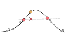
(a) KNN

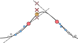
(b) DNNR

Figure 1: (a) An illustration of KNN regression. To predict a value for a query (circle with question mark), the target values of the nearest points (red circles) are averaged. KNN’s prediction is marked by the red cross. The other data points (gray circles) are not used for prediction. (b) Similar illustration of DNNR. The local gradient (gray dashed line) is estimated for each neighbor and a target value is interpolated linearly (light red crosses). The final prediction (red cross) is the average of these interpolated values.

2 Related Work

KNN  is a non-parametric model based on a simple voting decision rule where the target of a given point is predicted by averaging the targets of neighboring samples (Cover & Hart, 1967). For an introduction to KNN, we refer the reader to (Chen & Shah, 2018).

Numerous methods have been proposed to improve this simple decision rule. (Kulkarni & Posner, 1995; Chaudhuri & Dasgupta, 2014) investigated the KNN convergence rate under different sampling conditions while (Balsubramani et al., 2019) and (Wettschereck & Dietterich, 1993) proposed different methods for an adaptive choice of $k$.

Although the choice of the number of neighbors is critical, it is not the only factor governing KNN performance. A large subset of the KNN literature proposed techniques for the choice of the distance metric that defines the neighborhood. (Cleary & Trigg, 1995) introduced an entropy-based distance metric, and (Wang et al., 2007) proposed an adaptive distance. Metric learning methods propose data-driven learning mechanisms for the distance function (Weinberger & Tesauro, 2007; Weinberger et al., 2006; Wang et al., 2018). A similar approach changes the data representation upon which the distance function operates via feature weighting or feature selection (Aha, 1998; Vivencio et al., 2007). (Bhatia & Vandana, 2010) provides a more comprehensive overview of the different KNN techniques. However, all these methods do not change how the prediction is being performed – all use an averaging scheme of the targets that effectively does not account for how the function changes within the local neighborhood.

A method that uses local changes is local linear regression (LL) (Fan, 1992). Similarly to KNN, local linear regression selects $k$-nearest neighbors and then fits a hyperplane locally. This differs from our proposed method as we fit the gradient for all nearest neighbors separately. The single hyperplane of LL regression assumes an identical gradient for each neighbor. We show results for LL regression in the quantitative evaluation.

Gradient Approximation  Estimating the gradient from data has been studied for various reasons, including variable selection and dimensionality reduction (Hristache et al., 2001; Mukherjee & Zhou, 2006). Several non-parametric methods exist to estimate the gradient from data (Fan & Gijbels, 1996; De Brabanter et al., 2013), and bounds of convergence already exist for some techniques (Berahas et al., 2021; Turner et al., 2010). An error bound on L1-penalized gradient approximation using KNN is derived in (Ben-Shabat & Gould, 2020) using local gradient approximation for 3D model reconstruction by fitting truncated jets in the KNN neighborhoods. (Ausset et al., 2021). The work also applied the estimated gradient to variable selection and gradient optimization problems, but did not utilize it to improve the prediction. As we will present in detail, our method combines non-parametric gradient estimation using KNN, Taylor expansion, and feature scaling for regression modeling. To our surprise, this combination was neither explored theoretically nor empirically before.

3 Method

Algorithm 1 Pseudocode of DNNR’s prediction for a query point $X$. The feature scaling is omitted in this pseudocode. The OLS function solves an ordinary-least-squares problem.

a query point $x$, train data $\{(X_{i},Y_{i})\}$, nearest neighbors $k$, nearest neighbors for gradient estimation $k^{\prime}$, range for target value $y_{\min},y_{\max}$: $M\leftarrow$nn(x, k) # $M$contains the indices of the $k$nearest neighbors predictions = [] each neighbor index m $\in M$A $\leftarrow$nn($X_{m},k^{\prime}$) # $A$contains indices of the $k^{\prime}$neighbors for $X_{m}$$\Delta\bm{X}\leftarrow{X}_{A}-x_{m}$$\Delta\bm{Y}\leftarrow{Y}_{A}-y_{m}$$\hat{\gamma}_{m}\leftarrow\text{OLS}(\Delta\bm{X},\Delta\bm{Y})$# $\hat{\gamma}_{m}$approximates the gradient $\hat{y}_{m}\leftarrow y_{m}+\hat{\gamma}(x_{m}-x)$predictions.append($\hat{y}_{m}$) $\hat{y}$= mean(predictions) clip($\hat{y},y_{\min},y_{\max}$)

Notation  We will consider the typical supervised regression problem. The training data is given as a set of $n$ tuples of data points and target values $\{(X_{1},Y_{1}),\ldots,(X_{n},Y_{n})\}$. We will denote the expected target value by $\eta(x)=\mathbb{E}[Y|X=x]$. A ball with radius $r$ around $x$ is given by $B_{x,r}$. For a ball around $x$ with exactly $k$ training points, we will use a $\#$ sign as in $B_{{\bm{x}},\#k}$. We summarize our notation in the Appendix Table 4.

DNNR  Vanilla KNN predicts the target of a given datapoint $x$ by averaging the targets of nearby training points:

$$\eta_{\text{KNN}}(x)=\frac{1}{k}\sum_{\mathclap{X_{m}\in B_{x,\#k}}}Y_{m}.$$ (1)

This simple averaging scheme can be seen as a zeroth-term Taylor expansion around the inference point. If we would know the gradient of the function $\eta$, we could easily extend it to a first degree Taylor expansion:

$$\eta_{\text{known}\nabla}(x)=\frac{1}{k}\!\sum_{\mathclap{X_{m}\in B_{x,\#k}}}\left(Y_{m}+\nabla\eta(X_{m})(x-X_{m})\right).$$ (2)

Of course, we only have access to the training data, not the underlying target function. Therefore, we approximate the gradient using nearby points. We can approximate $\nabla\eta(X_{m})$ by solving a least-squares problem:

$$\hat{\gamma}_{m}=\arg\min_{\gamma_{m}}||A\gamma_{m}-q||,$$ (3)

where $\hat{\gamma}_{m}\in\mathbb{R}^{d}$ is the estimated gradient at point $X_{m}$, $A\in\mathbb{R}^{k^{\prime}\times d}$ contains the normalized differences $(X_{i}-X_{m})/h_{i}$ as row vectors, $h_{i}=||X_{i}-X_{m}||$, $k^{\prime}$ is the number of points used to approximate the gradient, $i$ indexes these $k^{\prime}$ nearby points around $X_{m}$ , and $q\in R^{k^{\prime}}$ denotes the differences in the labels $q=(Y_{i}-Y_{m})/h_{i}$. The result $\hat{\gamma}_{m}$ can then substitute the real gradient in equation (2) to yield the DNNR approximation:

$$\eta_{\text{DNNR}}(x)=\frac{1}{k}\sum_{\mathclap{X_{m}\in B_{x,\#k}}}\left(Y_{m}+\hat{\gamma}_{m}(x-X_{m})\right).$$ (4)

Using the approximate Taylor expansion, we aim to improve the prediction performance by also utilizing the local change in the function. The pseudocode of DNNR is listed in Algorithm 1. The algorithm can also be extended easily to higher-orders of a Taylor expansion. In the evaluation, we will report results using the diagonal of the Hessian, i.e. the elements corresponding to $\frac{\partial^{2}\eta}{\partial^{2}x_{i}}$.

Feature Weighting

Using an isotropic distance weighs each dimension equally. This way, a neighbor may be picked based on irrelevant dimensions. A simple improvement is to scale the feature dimensions as done in previous work (Weinberger & Tesauro, 2007). We use a common approach for a distance metric $d$ using a diagonal matrix $W$ to scale each dimension:

$$d(x_{i},x_{j})=(x_{i}-x_{j})^{T}W(x_{i},x_{j})$$ (5)

DNNR’s predictions are differentiable w.r.t. the input dimensions, so a loss can be backpropagated to the scaling matrix $W$ and optimized using gradient decent. Inspired by the Taylor theorem, we require that nearby points predict each other well while predictions of far points may come with a larger error. Therefore, the loss enforces a correlation between distance and the prediction error:

$$\begin{split}W^{*}=\arg\min_{W}\sum_{i,j\in I}\text{corr}\big{(}&d(X_{i},X_{j}),\\[-10.0pt] &\left|Y_{i}-\hat{\eta}_{\text{DNNR}}(X_{\text{nn}(i,k^{\prime})})\right|\big{)},\end{split}$$ (6)

where $I$ is an index set of nearby points, and corr denotes the Pearson correlation coefficient.

At first sight, an alternative might have been minimizing the prediction’s mean squared error (MSE). However, minimizing the MSE would not alter the scaling, as the prediction is scale-invariant, i.e. downscaling a dimension will increase the gradient, and the prediction will stay the same. Therefore, a spatial inductive bias in equation 6 is needed.

4 Theoretical Analysis

We focus on the point-wise error estimate of DNNR vs. KNN regression. The proof contains two parts: the approximation error of the gradient and the point-wise prediction error. In Appendix C.2, we show that:

Lemma 1

Let $f:D\subset\mathbb{R}^{d}\to\mathbb{R}$ be of class $C^{\mu}$, $a\in D$, and $\mathcal{B}(a)\subset D$ be some neighborhood of a. Suppose that around point $a$ we have $m$ neighboring points $v_{k}$, $k=1,\ldots,m$ with a, $v_{1},\ldots,v_{m}\in\mathcal{B}(a)\subset D$. Suppose further that all $\mu$-th order derivatives are Lipschitz, $i\in 1\ldots\mu$: $\frac{\partial^{i}f}{\partial a_{1}^{l_{1}}\ldots\partial a_{d}^{l_{d}}}\in Lip_{\vartheta_{i}}(\mathcal{B}(a))$ where $l_{1}+\ldots+l_{d}=i$ and we approximate the gradient locally at $a$ by $\hat{\gamma}=E_{1}\hat{\omega}$ via the least-squares solution $\hat{\omega}=\arg\min_{\omega\in\mathbb{R}^{d}}||A\omega-q||$, where

$$A\!=\!\begin{pmatrix}\nu_{1}^{T}&\nu_{1*}^{T}\\ \nu_{2}^{T}&\nu_{2*}^{T}\\ \vdots\\ \nu_{m}^{T}&\nu_{m*}^{T}\\ \end{pmatrix},\quad q\!=\!\begin{pmatrix}\!\frac{f(a+h_{1}\nu_{1})-f(a)}{h_{1}}\\ \frac{f(a+h_{2}\nu_{2})-f(a)}{h_{2}}\\ \vdots\\ \frac{f(a+h_{m}\nu_{m})-f(a)}{h_{m}}\\ \end{pmatrix},$$ (7)

$A\!\in\!\mathbb{R}^{m\times p}$, $q\!\in\!\mathbb{R}^{m}$, $E_{1}=\begin{pmatrix}I_{d}&0\end{pmatrix}\in\mathbb{R}^{d\times p}$, $h_{k}=||v_{k}-a||$ with $h_{k}\nu_{k}=v_{k}-a$; $\nu_{k}^{T}=(\nu_{1_{k}},\ldots,\nu_{d_{k}})$, $\nu_{k*}^{T}$ denotes higher-order terms $\nu_{k*}^{T}=\begin{pmatrix}\frac{h_{k}^{\mu^{\prime}-1}}{\mu^{\prime}!}\binom{\mu^{\prime}}{l_{1},\ldots,l_{d}}\prod_{i_{1}}^{d}\nu_{i}^{k_{i}}\end{pmatrix}_{2\leq\mu^{\prime}\leq\mu,l_{1}+\ldots l_{d}=\mu^{\prime}}$ and $p=\sum_{i=1}^{\mu}\frac{(d+\mu)!}{d!}$. Then a bound on the error in the least-squares gradient estimate is given by:

$$||\nabla f(a)-\hat{\gamma}||_{2}\leq\frac{\vartheta_{\max}h_{\max}^{\mu}}{\sigma_{1}(\mu+1)!}\sqrt{\sum_{i=1}^{m}||\nu_{i}||_{1}^{2\mu}},$$ (8)

where $\sigma_{1}$ is the smallest singular value of A, which is assumed to have $\text{rank}(A)=p$, $\vartheta_{\max}=\max_{i\in 1\ldots k}\vartheta_{i}$ and $h_{\max}=\max_{1\leq k\leq m}h_{k}$.

This lemma extends a result from the two-dimensional case (Turner et al., 2010). The gradient approximation depends on the Lipschitz constant $\vartheta_{\max}$, the distance to the neighbors $h_{\max}$, and the smallest singular value $\sigma_{1}$ of the normed differences $A$. The lemma also shows that by accounting for higher-order terms, e.g. picking $\mu>1$, the gradient approximation can be made more accurate.

The following theorem is based on Theorem 3.3.1 in (Chen & Shah, 2018). We built on the same assumptions except requiring Lipschitz instead of Hölder continuity.

Technical Assumptions ($\bm{A}_{\mathcal{X},\rho,\mathbb{P}_{X}}^{\text{technical}}$):  The feature space $\mathcal{X}$ and distance $\rho$ form a separable metric space. The feature distribution $\mathbb{P}_{X}$ is a Borel probability measure.

Assumption Besicovitch($\bm{A}_{\eta}^{\text{Besicovitch}}$):  The regression function $\eta$ satisfied the Besicovitch condition if $\lim_{r\downarrow 0}\mathbb{E}[Y|X\in B_{x,r}]\!=\!\eta(x)$ for $x$ almost everywhere w.r.t. $\mathbb{P}_{X}$.

Assumption Lipschitz ($\bm{A}_{\eta}^{\text{Lipschitz}(\vartheta_{\max})}$):  The regression function $\eta$ is Lipschitz continuous with parameter $\vartheta_{\max}$ if $|\eta(x)-\eta(x^{\prime})|\leq\vartheta_{\max}\rho(x,x^{\prime})$ for all $x,x^{\prime}\in\mathcal{X}$.

Using Lemma 1, we prove the following theorem in Appendix C.2:

Theorem 1

(DNNR pointwise error) Under assumptions $\bm{A}_{\mathcal{X},\rho,\mathbb{P}_{X}}^{\text{technical}}$ and $\bm{A}_{\eta}^{\text{Besicovitch}}$, let $x\in\text{supp}(\mathbb{P}_{X})$ be a feature vector, $\varepsilon>0$ be an error tolerance in estimating the expected label $\eta(x)=\mathbb{E}[Y|X=x]$, and $\delta\in(0,1)$ be a probability tolerance. Suppose that $Y\in[y_{\min},y_{\max}]$ for some constants $y_{\min}$ and $y_{\max}$. There exists a threshold distance $h_{\text{DNNR}}^{*}\in(0,\inf)$ such that for any smaller distance $h\in(0,h^{*})$, if the number of training points $n$ satisfies:

$$n\geq\frac{8}{\mathbb{P}_{X}(B_{x,h})}\log\frac{2}{\delta},$$ (9)

and the number of nearest neighbors satisfies

$$\frac{2(y_{\max}-y_{\min})^{2}}{\varepsilon^{2}}\log\frac{4}{\delta}\leq k\leq\frac{1}{2}n\mathbb{P}_{X}(B_{x,h}),$$ (10)

then with probability at least $1-\delta$ over randomness in sampling the training data, DNNR regression at point $x$ has error

$$|\hat{\eta}_{\text{DNNR}}(x)-\eta(x)|\leq\varepsilon.$$ (11)

If we know that $\bm{A}_{\eta}^{\text{Lipschitz}(\vartheta_{\max})}$ also holds, we can pick $h_{\text{DNNR}}^{*}$ as:

$$h_{\text{DNNR}}^{*}=\sqrt{\frac{\varepsilon}{\vartheta_{\max}\left(1+\tau\right)}},$$ (12)

where $\tau\!=\!\mathbb{E}\left[\frac{\sqrt{\sum_{i=1}^{m}||\nu_{i}||_{1}^{2\mu}}}{\sigma_{1}}\>\big{|}\>X\in B_{x,h}\right]$. $\nu$, $\sigma_{1}$, and $\vartheta_{\max}$ are defined as in Lemma 1.

The theorem states that we can bound the point-wise error locally with a high probability given that the conditions on $n$ and $k$ are fulfilled. Theorem 3.3.1 from (Chen & Shah, 2018) provides a KNN regression point-wise error bound (their theorem is in turn based on (Chaudhuri & Dasgupta, 2014)). For KNN, the restriction on the maximum distance $h_{\text{KNN}}^{*}=\frac{\varepsilon}{2\vartheta_{\max}}$, while the other conditions on sample size and probability are identical. To compare DNNR and KNN, it is beneficial to solve for the error tolerance $\varepsilon$.

$$\varepsilon_{\text{DNNR}}=h_{\text{DNNR}}^{2}{\vartheta_{\max}\left(1+\tau\right)},$$ (13)

and for KNN:

$$\varepsilon_{\text{KNN}}=2\vartheta_{\max}h_{\text{KNN}}.$$ (14)

The influence of the different variables is as follows:

• Both depend on the Lipschitz constant $\vartheta_{\max}$ linearly.

• Distance to nearest neighbors: $h_{\max}$ vs $h_{\max}^{2}$. For DNNR, the error decreases quadratically in $h_{\max}$. When $h_{\max}$ becomes small, $h_{\max}^{2}$ will be even smaller.

• For DNNR, $\tau$ represents the error in estimating the gradient. As long $\tau<\frac{2}{h_{\max}}-1$, the error tolerance of DNNR will be lower than for KNN. As $\tau\propto\frac{1}{\sigma_{1}}$, an ill-conditioned matrix $A$ might increase DNNR’s error.

5 Experiments

We compared DNNR against other methods, including state-of-the-art gradient boosting methods. First, we discuss which baselines we compared against and the general experimental setup. Then, we present large-scale quantitative evaluations followed by an ablation study and further qualitative analyses.

5.1 Setup

We compared DNNR against state-of-the-art boosting methods (CatBoost, XGBoost, Gradient Boosted Trees (Dorogush et al., 2018; Chen & Guestrin, 2016)) and classical methods such as (KNN, multi-layer perceptron (MLP), Random Forest). We also included KNN-Scaled, which uses DNNR’s feature weighting but KNN’s averaging scheme.

We used standard-scaling for all datasets (zero mean, unit variance per dimension). Each model was optimized using a grid search over multiple parameters, and the models were refit using their best parameters on the validation data before test inference, except for TabNet (Arik & Pfister, 2021) (for details see Appendix D). We ensured that each method had a comparable search space. Approximately 4.1k CPU hours were used to run the experiments. For the larger benchmarks (Feynman and PMLB), we followed the setup in (Cava et al., 2021). Our baselines report similar or slightly better performance than on SRBench.

5.2 Quantitative Experiments

Table 1: The MSE on eight regression datasets averaged over 10-folds. The best performing values are marked as bold. The standard deviations are given after the ± signs. For the Sarcos dataset, we only evaluate on the given test set.

	Protein	CO2Emission	California	Yacht	Airfoil	Concrete	NOxEmission	Sarcos
CatBoost	11.82 ± 0.33	1.11 ± 0.40	0.19 ± 0.01	0.25 ± 0.25	1.26 ± 0.24	14.00 ± 5.35	14.65 ± 1.00	1.313
Grad. B. Trees	12.15 ± 0.41	1.25 ± 0.44	0.20 ± 0.01	0.33 ± 0.15	1.76 ± 0.51	16.03 ± 6.13	15.60 ± 1.00	1.813
LGBM	12.74 ± 0.35	1.17 ± 0.41	0.19 ± 0.01	6.86 ± 9.10	2.03 ± 0.38	16.10 ± 5.11	15.66 ± 1.00	1.613
MLP	14.34 ± 0.44	1.23 ± 0.47	0.35 ± 0.26	4.34 ± 10.21	10.17 ± 3.01	35.27 ± 12.17	19.91 ± 1.82	1.277
Rand. Forest	11.80 ± 0.25	1.12 ± 0.43	0.23 ± 0.02	1.13 ± 0.73	2.81 ± 0.66	22.75 ± 5.64	16.35 ± 1.03	2.264
XGBoost	12.01 ± 0.28	1.21 ± 0.44	0.20 ± 0.02	0.26 ± 0.16	1.63 ± 0.40	16.76 ± 6.68	14.99 ± 0.98	1.824
KNN	13.39 ± 0.37	1.17 ± 0.43	0.39 ± 0.03	68.46 ± 51.11	4.25 ± 0.96	60.76 ± 14.19	17.37 ± 1.26	1.752
KNN-Scaled	12.54 ± 0.57	1.20 ± 0.44	0.19 ± 0.02	2.66 ± 1.92	4.14 ± 0.94	40.25 ± 7.00	15.41 ± 1.21	1.770
LL	14.07 ± 0.18	1.20 ± 0.46	0.33 ± 0.07	50.83 ± 14.81	7.04 ± 1.39	51.40 ± 10.50	16.69 ± 1.10	0.792
LL-Scaled	12.90 ± 0.29	1.10 ± 0.43	0.21 ± 0.02	2.47 ± 1.70	3.53 ± 1.24	32.54 ± 6.33	14.57 ± 0.96	0.786
Tabnet	17.02 ± 2.68	1.22 ± 0.38	0.39 ± 0.04	2.83 ± 2.59	9.98 ± 3.04	43.73 ± 14.59	12.97 ± 0.92	1.304
DNNR	12.31 ± 0.35	1.12 ± 0.47	0.19 ± 0.02	1.05 ± 0.63	2.83 ± 0.60	36.52 ± 18.03	13.34 ± 0.96	0.708
DNNR-2 ord.	11.64 ± 0.44	1.24 ± 0.50	0.22 ± 0.02	0.48 ± 0.43	2.30 ± 0.48	28.35 ± 13.47	15.61 ± 1.94	0.727

Benchmark Datasets:   The goal of this benchmark is to inspect DNNR’s performance on eight real-world regression datasets: Yacht, California, Protein, Airfoil, Concrete, Sarcos, CO2 Emissions, and NOX emissions. The last two datasets are part of the Gas Emission dataset. All datasets were taken from the UCI repository (Dua & Graff, 2017), except California (Kelley Pace & Barry, 1997) and Sarcos (Rasmussen & Williams, 2006). These datasets were also used in previous work (Bui et al., 2016). Some of the datasets also come with discrete features (Yacht, Airfoil), which challenges DNNR’s assumption of continuity. All the datasets were evaluated using a 10-fold split, except for the Sarcos dataset which comes with a predefined test set. Additionally, we fixed the data leakage in the Sarcos dataset by removing all test data points from the training set.

In Table 1, we report the averaged mean squared error (MSE) over the 10-folds for each dataset and model. Overall, CatBoost is the best performing method. We find that DNNR achieves the best performance on the Sarcos and California datasets and the second order achieves the best performance on Protein. For NOxEmissions, CO²Emissions, and Protein, DNNR is within 5% percentage difference to the best performing method (see Table 3). Discrete features violate DNNR’s assumptions, which affect its performance, as the results on Airfoil and Yacht indicate.

Discrete features can render the Taylor approximation meaningless, e.g. all neighbors may have the same value in one dimension rendering the gradient zero, or a linear approximation may not be sufficient when values exhibit large jumps. Interestingly, the second-order DNNR yields better results on the Airfoil and Concrete datasets, presumably because the second order is a better approximator of sharp gradients.

On the other datasets, DNNR delivers a significant improvement over KNN and also over KNN with DNNR feature scaling (KNN-Scaled).

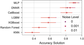
Figure 2: Accuracy on the Feynman Symbolic Regression Database under three levels of noise. The marks show the percentage of solutions with $R^{2}>0.999$ . The bars denote $95\%$ confidence intervals.

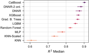
Figure 3: Results on the PMLB benchmark. The markers show the median $R^{2}$ performance over all datasets runs. Horizontal bars indicate the 95% bootstrapped confidence interval.

Feynman Benchmark  As second benchmark, we selected the Feynman Symbolic Regression Database, which consists of 119 datasets sampled from classical and quantum physics equations (Udrescu & Tegmark, 2020). These equations are continuous differentiable functions. The difficulty can be increased by adding noise.

The evaluation for the Feynman benchmark was executed with 10 different splits for each dataset and noise level (std=0, 0.001, 0.01) – similar to (Cava et al., 2021). For the first split, we divided the data into 70/5/25% train, validation, and test sets. The hyperparameter tuning was done with validation data of the first split. Then the models were refit using the best parameters and evaluated on the 25% test set. Subsequent splits (75/25% train/test) then used these hyperparameters.

For the Feynman benchmark, accuracy is defined as the percentage of datasets which were solved with a coefficient of determination $R^{2}>0.999$. We report this accuracy in Figure 2. DNNR is the second-best performing method after MLP. CatBoost’s performance is also notable with an accuracy of more than 80%. The different noise levels had minor effects on the methods.

PMLB Benchmark  The PMLB benchmark contains real and synthetic datasets with categorical features, discrete targets, and noisy data in general. In total, we used 133 PMLB datasets. The evaluation setup for the PMLB datasets was similar to the Feynman benchmark. Figure 3 shows the median $R^{2}$ performance of the different models with a 95% confidence interval. CatBoost is the best performing method with an $R^{2}$ median $>0.9$ with DNNR second order closely in second position. DNNR, XGBoost, and Gradient Boosted Trees perform similarly well. The worst-performing method is KNN regression. While adding feature weighting (KNN-Scaled) improves the $R^{2}$ median considerably by over 0.1, only DNNR’s additional use of gradient information yields results comparable to gradient boosting methods.

5.3 Ablation

In the previous evaluations, we already included KNN-Scaled to measure the effect of the scaling versus the gradient information. We dissected DNNR even further and tested various design alternatives: such as scaling of the neighborhood (MLKR (Weinberger & Tesauro, 2007)) and regularization on the gradient estimation (Lasso (Ausset et al., 2021)). We based this analysis on the Airfoil, Concrete, and 5000 samples from Friedman-1 datasets (see Section 5.4). As before, we conducted a hyperparameters sweep for each model configuration and used a 10-fold validation for each dataset.

For the Concrete and Friedman-1 datasets, using only gradient information and no feature scaling (DNNR-Unsc.) already improved over KNN’s performance. For the Airfoil dataset, which contains categorical features, using gradients without scaling (DNNR-Unsc.) lead to worse results. We find that MLKR improves KNN’s performance better than DNNR’s scaling for KNN. However, when using gradient estimation, MLKR is less suitable as can be seen in the difference between DNNR and DNNR-MLKR on Airfoil and Concrete. Furthermore, we would like to note that MLKR is also computationally more expensive than DNNR’s scaling as they use Gaussian kernels which results in a runtime quadratic in the number of samples. These results highlights that while the gradient information might be helpful for unscaled neighborhoods, scaling yields better gradients and results in better approximations.

Using Lasso regularization on the gradient estimation as done in (Ausset et al., 2021) did not perform well. We speculate that the regularization limits the gradient estimation. Future work might test if DNNR benefits from Lasso regularization in high-dimensional problems as motivated by the authors.

Table 2: Ablation study. We report the MSE for different variations of DNNR for three datasets.

	Airfoil	Concrete	Friedman-1
DNNR	2.83 ± 0.60	36.52 ± 18.03	0.01 ± 0.00
DNNR-Unsc.	4.82 ± 0.74	49.97 ± 13.59	1.03 ± 0.15
KNN-MLKR	3.32 ± 0.84	36.85 ± 9.89	0.40 ± 0.07
KNN-Scaled	4.14 ± 0.94	40.25 ± 7.00	7.27 ± 0.53
DNNR-MLKR	3.20 ± 1.08	1.5e13 ± 4e13	0.03 ± 0.00
KNN	4.25 ± 0.96	60.76 ± 14.19	3.93 ± 0.43
DNNR Rand.	24.38 ± 3.44	115.14 ± 20.52	6.07 ± 0.56
DNNR-Lasso	5.25 ± 1.05	40.24 ± 8.43	7.33 ± 0.52
DNNR-2 ord.	2.30 ± 0.48	28.35 ± 13.47	0.01 ± 0.00

5.4 Effect of noise, #samples, and #features

This analysis investigates how different data properties affect the model’s performance. Such an analysis requires a controlled environment: we used the Friedman-1 dataset (Friedman, 1991). This dataset is based on the following equation:

$$\begin{split}y(x)=10x_{3}+5x_{4}&+20\left(x_{2}\!-\!0.5\right)^{2}\\ &+10\sin{\left(\pi x_{0}x_{1}\right)}+s\epsilon,\end{split}$$ (15)

where $x_{i}$ is uniformly distributed in [0, 1], the noise $\epsilon$ is sampled from a standard normal distribution, and $s$ controls the variance of the noise. Unimportant features can be added by simply sampling $x_{j}\sim U(0,1)$. Friedman-1 allowed us to test the models under different sampling conditions: the number of samples, the magnitude of noise, and the number of unimportant features.

As defaults, we choose the number of samples = 5000, the number of features = 10, and the noise level = 0. Besides DNNR, we also evaluated Gradient Boosted Trees, CatBoost, Random Forest, MLP, and KNN. For each setting, we run a 5-fold evaluation (the hyperparameters of each methods are fitted on the first fold and then fixed for the remaining 4).

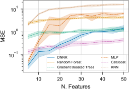
(a) Number of Features

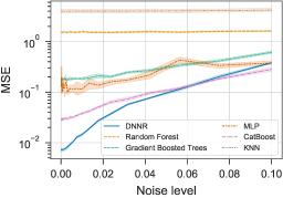
(b) Noise Level

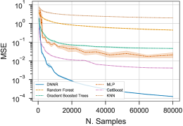
(c) Number of Samples

Figure 8: The effect of different parameters of the dataset. The results are obtains on the Friedman-1 dataset. The confidence intervals denote the standard derivation over multiple folds.

We report the effect of each condition in Appendix Figure 8. For the number of samples, we note that DNNR’s error declined rapidly. Second-best is CatBoost. For noise, we observed two groupings. While one group (MLP & KNN) performed poorly, their MSE did not increase when adding noise. For the better performing group (DNNR, Gradient Boosted Trees, CatBoost, Random Forest), the error did increase when adding noise. In this group, DNNR performed the best for low noise levels, but was beaten by CatBoost slightly for higher levels of noise.

Increasing the number of unimportant features impacted KNN and MLP particularly. DNNR dropped from being the best method to sharing the second place with Gradient Boosted Trees as the feature scaling cannot entirely mitigate the effect of unimportant features. Tree-based methods were barely affected, as they are adept at handling unimportant features and operate on the information gain of each feature.

5.5 Application of the theoretical bound

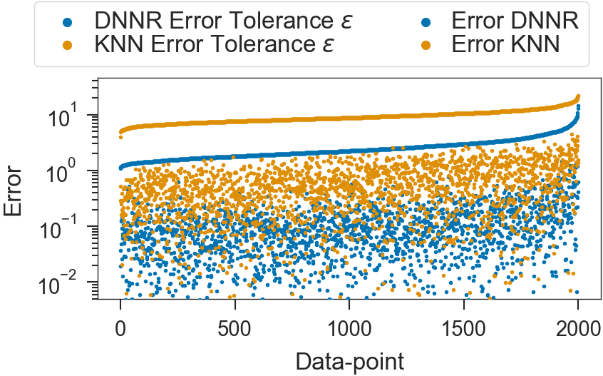
Figure 4: Comparison between the error bound of KNN (yellow) and DNNR (blue). On the x-axis, all test data points sorted by their error bounds are plotted. The DNNR performs better than KNN and the DNNR error bound is also lower.

Figure 5: Depicts the error tolerance versus the number of training samples for the Friedman-1 dataset. KNN requires multiple orders more training points to guarantee the same error tolerance.

In this evaluation, we analyze the error bounds from section 4. As dataset, we use the Friedman-1 dataset introduced before in section 5.4. The synthetic dataset allows sampling arbitrary points, thereby we can simulate also very dense neighborhoods.

First, we apply Theorem 1 to the dataset. We pick a probability tolerance of 0.95 ($\delta=0.05$), and a Lipschitz constant for equation (15) of $\vartheta_{\max}=40$. For DNNR, we estimate a value of $\tau\approx 5.59$ from the data. We show the dependency between error tolerance the number of samples required in Figure 5. In this exemplary calculation, KNN requires multiple orders of magnitude more training data than DNNR to achieve the same theoretical guarantee on the error tolerance. Still, even DNNR would require an unrealistic amount of samples, e.g. around $10^{15}$ for an error tolerance of $\varepsilon=0.1$.

As a more practical application, we investigated how local conditions, e.g. distance to the neighbors and the Lipschitz constant, influence the local prediction error. Therefore, we sampled a realistically sized train and test set (10.000 and 2.000 samples) and then compared the error tolerance for KNN and DNNR according to equations (13) and (14). For both methods, we choose $k=7$, and for the number of neighbors to approximate the gradient, we used $k^{\prime}=32$. We purposely violate the conditions on $k$ and $n$ of Theorem 1, as we want to analyze how applicable the estimated error tolerances are in a more realistic setting. In Figure 4, we sorted the 2000 test points according to the error tolerances of KNN and DNNR respectively. For both methods, we see that the error tolerances were strictly bound the actual errors by a gap of around one order of magnitude. We also observe that the error tolerances were correlated with the actual errors, e.g. as the error tolerances decrease, so does the actual error.

5.6 Feature importance & Inspecting a prediction

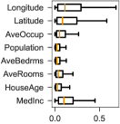
(a) Feature relevances

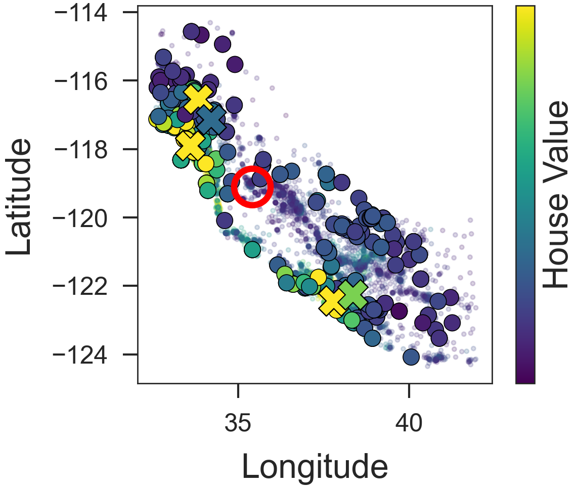
(b) Failure (error of 4.85)

Figure 6: (a) Feature relevance of DNNR Unscaled on the California Housing dataset. (b) A failure of DNNR Unscaled. The red circle marks the query point. The prediction is done by approximating the gradient locally for each nearest neighbors (crosses). The circles visualize the points used for gradient approximation. As DNNR Unscaled weights each dimension equally, it does not use spatially nearby points, even though longitude and latitude are scored important.

DNNR allows inspecting which neighbors were used for the prediction and how they contributed. For the following exemplary inspection, we use the California Housing dataset (Kelley Pace & Barry, 1997). The dataset’s dependent variable is the median house value per block group (a block group is an aggregation of a local area). The eight observational variables represent the location, median income, and information about the houses, such as average rooms or occupation. For this study, we analyzed DNNR Unscaled, i.e. DNNR without the feature scaling. We omitted the feature scaling, as the feature relevance would be impacted by the scaling and the DNNR with scaling is also performing so well that the error would be minor to inspect.

First, we can provide a simple local feature relevance score by multiplying the estimated gradient with the difference in the input:

$$\bm{\xi}_{m}=|({\bm{x}}-{\bm{x}}_{m})\odot\hat{\gamma}_{m}|,$$ (16)

where $x_{m}$ is the point where we estimate the gradient and $\hat{\gamma}_{m}$ the locally fitted gradient. This formulation of feature importance is analogous to a linear model where one would take $w\odot x$ (Molnar, 2019, sec. 5.1.). It is a known property that the gradient reflects the model’s sensitivity and can be used for feature importance, and variable selection (Mukherjee & Zhou, 2006; Guyon & Elisseeff, 2003). We show the distributions of the local feature importance in Figure 6(a).

The most important dimensions are longitude, latitude, and median income. We validate the local feature importance by applying it to variable selection. Using all dimensions, we get an MSE of around 0.34 (this is lower than in Table 1 as we do not use feature weighting). When deleting the three most important dimensions, the MSE increases to 0.99. However, keeping only the most important dimensions, the MSE slightly improves to 0.33. Therefore, we conclude that the feature importance has found the most important dimensions.

We now move on to inspect a failure case of DNNR. In Figure 6(b), we show how the neighborhood of a badly predicted point can be inspected. The prediction (red circle) is off by 4.85. From looking at the projection of the data to the longitude and latitude dimensions, we can see that the prediction is based on points (crosses) far away from the query. These points might have a similar number of bedrooms but differ in the location. As we found in the previous experiment, the latitude/longitude belong to the most important features. This inspection motivates the feature scaling once again, as DNNR Unscale weights all dimension equally, it selected the nearest neighbors using less relevant dimensions.

6 Conclusion, Limitations, and Future Work

Conclusion  DNNR showed that local datapoint gradients carry valuable information for prediction and can be exploited using a simple Taylor expansion to provide a significant performance boost over KNN regression. In large-scale evaluations, DNNR achieved comparable results to state-of-the-art complex gradient boosting models. An advantage of DNNR’s simplicity is that we can obtain error bounds by extending KNN’s theory. Our theoretical analysis illustrates the benefits of using DNNR over KNN. DNNR strikes a good balance between performance and transparency and may therefore be the method of choice in problems with elevated requirements for the system’s interpretability.

Limitations  Our evaluation of DNNR points to a potential limitation on discrete data. When features or targets have the same value, the gradient is zero and DNNR falls back to KNN’s decision. On partially discrete datasets DNNR performs always at least as well as KNN, see e.g. the results of DNNR and KNN on the Yacht dataset (Table 1). DNNR also inherits some limitations from KNN, such that the L2-metric might not represent similarities optimally.

Future Work  DNNR was designed for regression tasks but could be adapted for classification as well, e.g. by fitting the gradients of a logistic function as in (Mukherjee & Wu, 2006) or via label smoothing (Müller et al., 2019). An interesting future direction may be in extending DNNR specifically to symbolic regression by utilizing the estimated gradient information. Future work could also explore the use of DNNR for data augmentation, where points could be sampled, and the label computed estimated with the local gradient. Another research direction would be to tighten the theoretical bounds or to study the effect of scaling from a theoretical perspective.

Acknowledgments

We thank Maximilian Granz, Oana-Iuliana Popescu, Benjamin Wild, Luis Herrmann, and David Dormagen for fruitful discussion and feedback on our manuscript. We are also grateful for our reviewers’ feedback. LS was supported by the Elsa-Neumann Scholarship of the state of Berlin. We thank the HPC Service of ZEDAT, Freie Universität Berlin, for generous allocations of computation time (Bennett et al., 2020).

Appendix A Figures

(a) Sample 1305: Error of 4.85

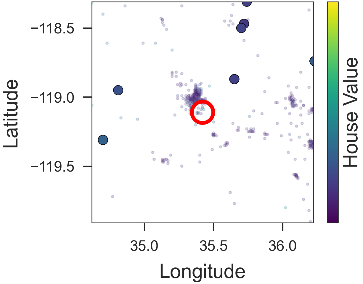
(b) Zoom of 1305

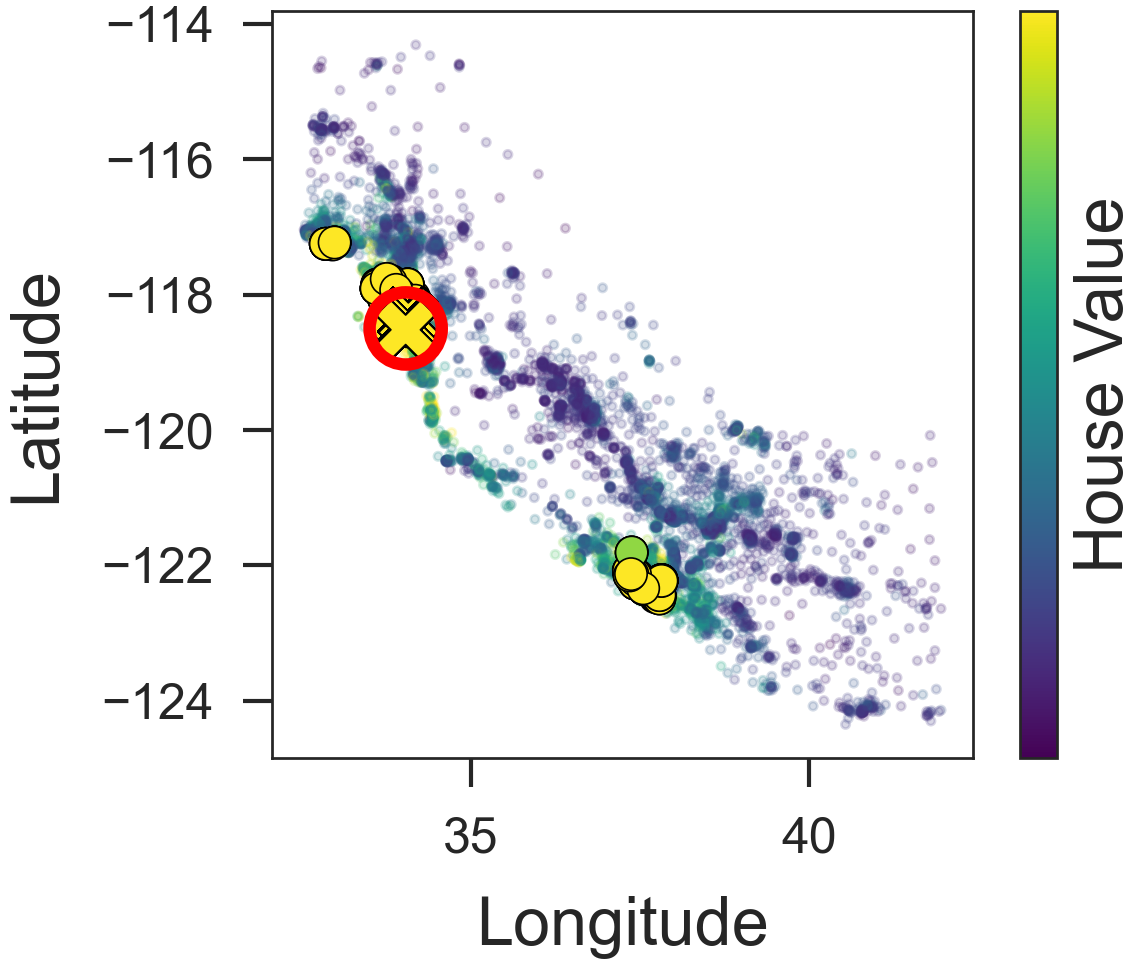
(c) Sample 1220 (Error 0.02)

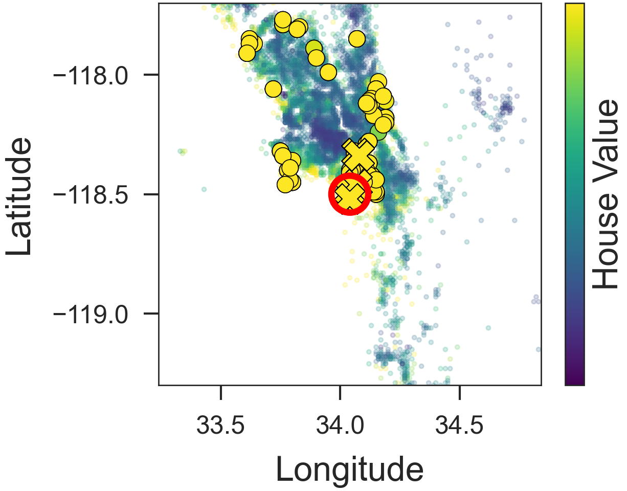
(d) Zoom of 1220

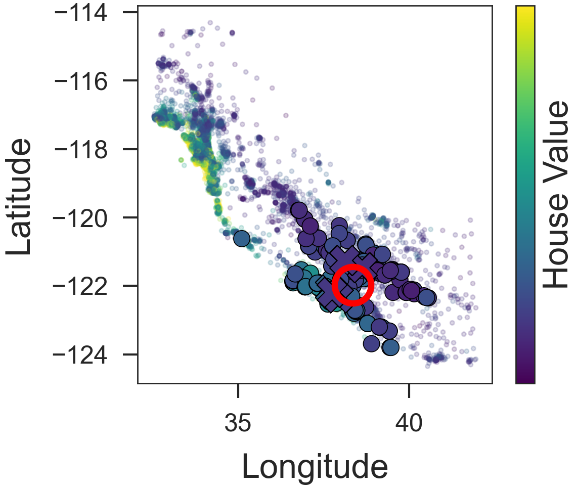
(e) Sample 1081 (Error 0.13)

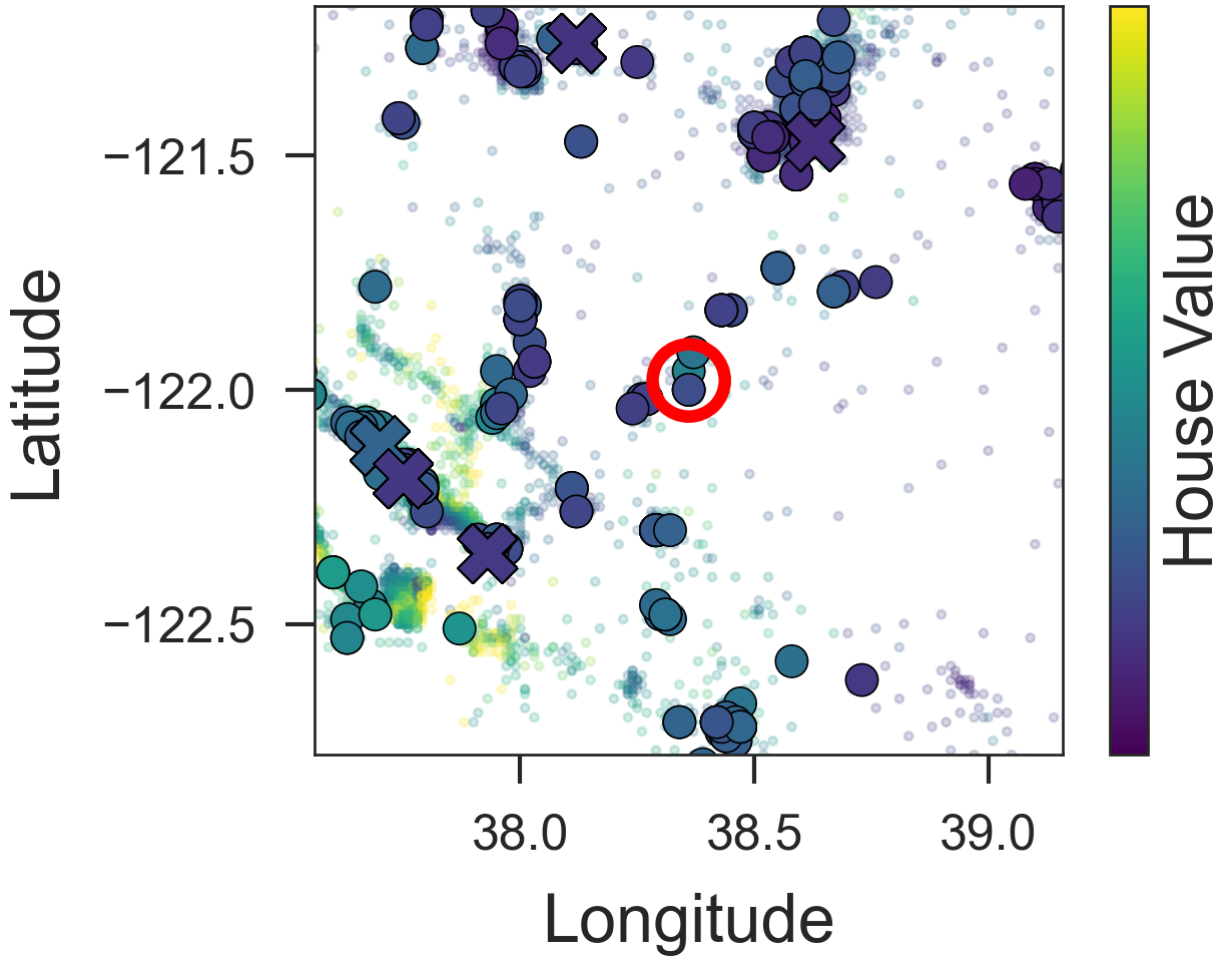
(f) Zoom of 1081

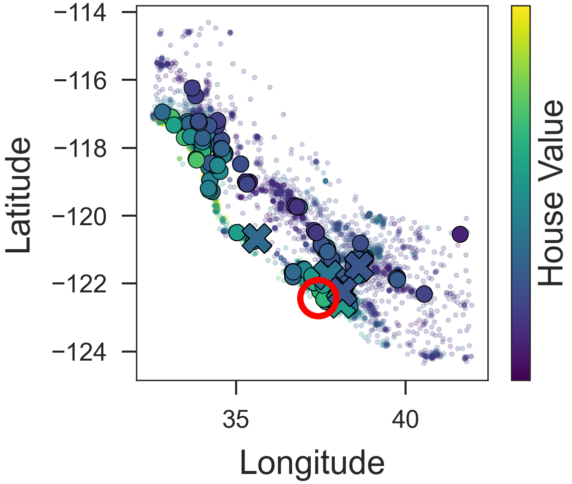
(g) Sample 393 (Error 1.01)

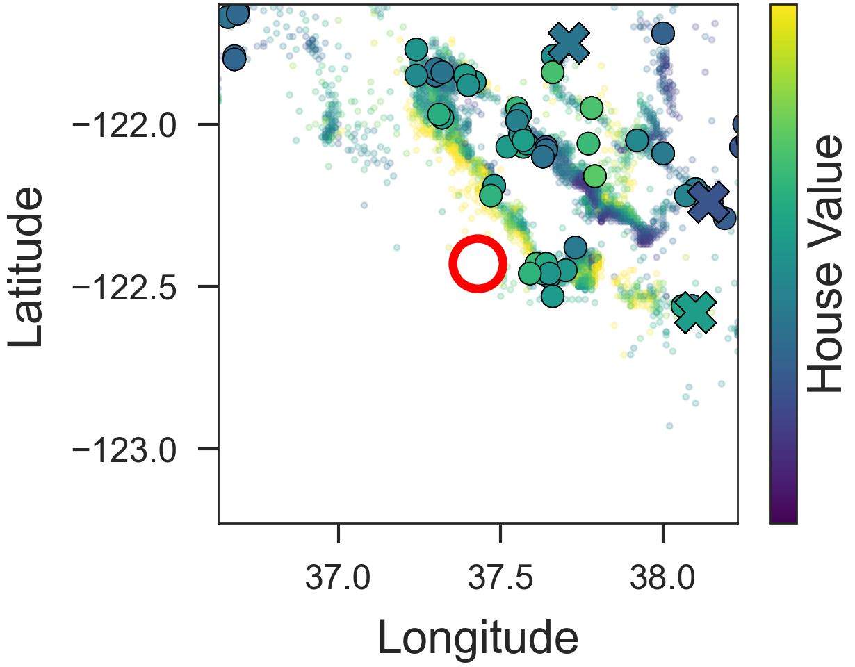
(h) Zoom of 393

Figure 7: The selected neighbors for different queries on the California dataset. The red circle marks the query point. The prediction is done by approximating the gradient locally for each nearest neighbors (crosses). The filled circles visualize the points used for gradient approximation. The neighbors are further away for higher errors (a) & (g) while close to the query for lower errors (c) & (e).

Appendix B Tables

Table 3: Mean percentage difference from the best performing model on each dataset.

	Protein	CO2Emission	California	Yacht	Airfoil	Concrete	NOxEmission	Sarcos
CatBoost	1.54%	1.09%	0.00%	0.00%	0.00%	0.00%	12.91%	85.45%
Grad. B. Trees	4.42%	13.71%	7.94%	32.14%	39.32%	14.53%	20.26%	156.07%
KNN	15.03%	6.63%	108.47%	27065.48%	236.23%	334.12%	33.91%	147.46%
KNN-neigh	7.76%	8.90%	2.65%	953.97%	227.69%	187.56%	18.79%	150.00%
LGBM	9.51%	6.09%	3.17%	2623.41%	60.36%	15.05%	20.74%	127.82%
LL	20.93%	8.99%	72.49%	20072.22%	457.28%	267.28%	28.69%	11.86%
LL-neigh	10.83%	0.00%	12.70%	880.95%	179.35%	132.46%	12.35%	11.02%
MLP	23.22%	11.99%	84.13%	1623.02%	704.43%	151.99%	53.46%	80.37%
Random Forest	1.39%	1.54%	21.69%	348.81%	122.15%	62.53%	26.08%	219.77%
Tabnet	46.25%	10.63%	108.47%	1024.21%	689.79%	212.47%	0.00%	84.18%
XGBoost	3.17%	9.99%	6.35%	2.78%	28.72%	19.73%	15.54%	157.63%
DNNR-2 ord.	0.00%	12.35%	13.76%	88.89%	81.96%	102.52%	20.37%	2.68%
DNNR	5.79%	1.27%	0.00%	315.08%	123.58%	160.93%	2.86%	0.00%

Appendix C Approximation Bounds

Notation	Meaning
$x$	An input vector
$X$	The random variable of the input
$Y$	The random variable of the output
$k$	The number of nearest neighbors
$k^{\prime}$	The number of neighbors to estimate the gradient
$\eta(x)$	The expected target value: $\eta(x)=\mathbb{E}[Y|X=x]$
$\nabla\eta(x)$	The gradient of $\eta(x)$ w.r.t. $x$
$\eta_{\text{KNN}}(x)$	Estimated regression function for KNN regression
$\eta_{\text{DNNR}}(x)$	Estimated regression function for DNNR
$\text{nn}(x,k)$	Returns the indices of the $k$ nearest neighbors of $x$
$\hat{Y}_{m,x}$	Estimated regression value for $x$ from point $X_{m}$
$\vartheta_{\max}$	Maximum Lipschitz constant
$A$	Matrix to estimate the gradient using OLS
$\sigma_{1}$	Smallest singular value of $A$
$C^{\mu}$	Set of $\mu$ times differentiable continuous functions
$(v\cdot\nabla)^{\mu}f$	The $\mu$-order directional derivative of f w.r.t $v$
$\mathbb{E}_{n}[.]$	Expectation over $n$ training points $(X_{i},Y_{i})_{1\leq i\leq n}$
${\hat{\gamma}}_{m}$	Locally estimated gradient for point $m$.
${\hat{\omega}}_{m}$	Locally estimated gradient and higher order terms
$\varepsilon$	The error tolerance
$\delta$	Probability tolerance
$h_{m}$	Distance between $x$ and point $X_{m}$
$\rho(x,x^{\prime})$	Distance metric

Table 4: Notation used in this work.

The proof of the approximation bounds of DANN extends the the proof of KNN approximation bounds given in (Chen & Shah, 2018, p. 68ff.) by a Taylor Approximation. For the approximation of the gradient, we will rely on results given in (Turner et al., 2010).

Notation  Our notation follows the one given in (Chen & Shah, 2018):

C.1 General Properties

We list here some inequalities used in the later proof.

Jensen’s Inequality  Given a random variable $X$ and a convex function $f(X)$ then:

$$f(\mathbb{E}[X])\leq\mathbb{E}[f(X)].$$ (17)

Hoeffding’s Inequality  Let $X_{1},\ldots,X_{k}$ be independent random variables bounded between $[a,b]$. The empirical mean is given by: $\bar{X}=\frac{1}{k}(X_{1}+\ldots+X_{k})$. Then:

$$\mathbb{P}(\left|\bar{X}-\mathbb{E}[\bar{X}]\right|>t)\leq 2\exp\left(-\frac{2kt^{2}}{(b-a)^{2}}\right)$$ (18)

Chernoff Bound for Binomial distribution  Let $X=\sum_{i=1}^{n}X_{i}$ be a sum of $n$ independent binary random variable each $X_{i}=1$ with probability $p_{i}$. Let $\mu=\mathbb{E}[X]=\sum_{i=1}^{k}p_{i}=n\bar{p}$, where $\bar{p}=\frac{1}{n}\sum_{i=1}^{k}p_{i}$. Then

$$\mathbb{P}(X\leq(1-\delta)\mu)\leq\exp(-\mu\delta^{2}/2).$$ (19)

C.2 Gradient Approximation

Here, we first proof two lemmas for bounding the gradient. They generalize the proof in (Turner et al., 2010, section 3.1) from 2 to $d$-dimensions.

The first Lemma bounds terms of a Taylor series and is need for the proof of Lemma .

Lemma 2

Let $f:D\subset\mathbb{R}^{d}\to\mathbb{R}$ be of class $C^{\mu}$, $a\in D$, and $B(a)\subset D$ some neighborhood of a. Suppose that for $i=0,1,\ldots,n$ we have $\frac{\partial^{\mu}f}{\partial^{\mu}a}\in Lip_{\vartheta_{i}}(B(a))$ and $\vartheta_{\max}=\max_{i\in 1,\ldots\mu}\vartheta_{i}$. Then for any $a+h\nu\in B(a)$ with $||\nu||=1$

$$\left|\sum^{\mu}_{k=1}\frac{h^{k-1}}{k!}(\nu\cdot\nabla)^{k}f(a)-\frac{f(a+h\nu)-f(a)}{h}\right|\leq\frac{h^{\mu}}{(\mu+1)!}\vartheta_{\max}||v||_{1}^{\mu}.$$ (20)

Proof Lemma 2. The proof starts with rearranging the Taylor Series which is given here:

$$f(a+h\nu)=f(a)+h\frac{(\nu\cdot\nabla)f(a)}{1!}+\ldots+h^{\mu}\frac{(\nu\cdot\nabla)^{\mu}f(a)}{\mu!}+R_{\mu}.$$ (21)

The remainder $R_{\mu}$ has the following form:

$$R_{\mu}=\frac{h^{\mu+1}}{\mu!}\int_{0}^{1}(1-t)^{\mu}(\nu\cdot\nabla)^{\mu+1}f(a+th\nu)dt.$$ (22)

By dividing by $h$ and rearanging some terms, we have:

$$\frac{f(a+h\nu)-f(a)}{h}-\sum_{k=1}^{\mu-1}\frac{h^{k-1}}{k!}(\nu\cdot\nabla)^{k}f(a)=\frac{R_{\mu-1}}{h}.$$ (23)

Now, we add the same quantity to both sides of the previous equation, using $\int_{0}^{1}(1-t)^{\mu-1}dt=\frac{1}{\mu}$:

$$\frac{h^{\mu-1}}{\mu!} (\nu\cdot\nabla)^{\mu}f(a)-\frac{f(a+h\nu)-f(a)}{h}+\sum_{k=1}^{\mu-1}\frac{h^{k-1}}{k!}(\nu\cdot\nabla)^{k}f(a)$$

$$=\frac{h^{\mu-1}}{(\mu-1)!}\int_{0}^{1}(1-t)^{\mu-1}\Big{\{}(\nu\cdot\nabla)^{\mu}f(a)-(\nu\cdot\nabla)^{\mu}f(a+th\nu)\Big{\}}dt.$$

Therefore, we have:

$$\left|\sum_{k=1}^{\mu-1}\frac{h^{k-1}}{k!}(\nu\cdot\nabla)^{k}f(a)-\frac{f(a+h\nu)-f(a)}{h}\right|$$

$$= \left|\frac{h^{\mu-1}}{(\mu-1)!}\int_{0}^{1}(1-t)^{\mu-1}\Big{\{}(\nu\cdot\nabla)^{\mu}(f(a)-f(a+th\nu))\Big{\}}dt\right|$$

$$=\left|\frac{h^{\mu-1}}{(\mu-1)!}\int_{0}^{1}(1-t)^{\mu-1}\Big{\{}(\nu\cdot\nabla)^{\mu}(f(a)-f(a+th\nu))\Big{\}}dt\right|$$

$$\leq\frac{h^{\mu-1}}{(\mu-1)!}\int_{0}^{1}(1-t)^{\mu-1}\Big{|}\left(\nu\cdot\nabla\right)^{\mu}\left(f(a)-f(a+th\nu)\right)\Big{|}dt$$

$$\leq\frac{h^{\mu+1}}{(\mu+1)!}\vartheta_{\max}\left|\nu\right|_{1}^{\mu}.$$

In last step, we rewrote the $\mu$-th directional derivative using partial derivative and bounded it using the Lipschitz-continuity as follows:

$$|(\nu\cdot\nabla)^{\mu}(f(a)-f(a+th\nu))|$$

$$=\left|\sum_{k_{1}+\ldots+k_{d}=\mu}\binom{\mu}{k_{1},\ldots,k_{d}}\left(\prod_{i=1}^{d}\nu_{i}^{k_{i}}\right)\frac{\partial^{\mu}(f(a)-f(a+th\nu))}{\partial a_{1}^{k_{1}}\cdot\ldots\cdot\partial a_{d}^{k_{d}}}\right|$$

$$=\sum_{k_{1}+\ldots+k_{d}=\mu}\binom{\mu}{k_{1},\ldots,k_{d}}\left(\prod_{i=1}^{d}\left|\nu_{i}^{k_{i}}\right|\right)\frac{\partial^{\mu}\left|(f(a)-f(a+th\nu))\right|}{\partial a_{1}^{k_{1}}\cdot\ldots\cdot\partial a_{d}^{k_{d}}}$$

$$\leq\sum_{k_{1}+\ldots+k_{d}=\mu}\binom{\mu}{k_{1},\ldots,k_{d}}\left(\prod_{i=1}^{d}\left|\nu_{i}^{k_{i}}\right|\right)\vartheta_{\max}|a-a+th\nu|\quad\text{(Lipschitz continuity of order $\mu$)}$$

$$=\vartheta_{\max}|th\nu|\left(\left|\nu_{1}\right|+\ldots+\left|\nu_{d}\right|\right)^{\mu}\quad\quad\text{(Multinomial theorem)}$$

$$=\vartheta_{\max}|th|\left|\nu\right|_{1}^{\mu}.\quad\quad$$

This finishes the proof of Lemma 2. $\square$

Lemma 3

Let $f:D\subset\mathbb{R}^{d}\to\mathbb{R}$ be of class $C^{\mu}$, $a\in D$, and $B(a)\subset D$ be some neighborhood of a. Suppose around point $a$ we have $m$ neighboring points $v_{k}$, $k=1,\ldots,m$ with a, $v_{1},\ldots,v_{m}\in B(a)\subset D$. Suppose further that $\frac{\partial^{\mu}f}{\partial a_{1}^{l_{1}}\ldots\partial a_{d}^{l_{d}}}\in Lip_{\vartheta_{\max}}(B(a))$ for $l_{1}+\ldots+l_{d}=\mu$, and we approximate the gradient locally at $a$ by $E_{1}\hat{\omega}$ via the least-squares solution $\hat{\omega}=\arg\min_{\omega\in\mathbb{R}^{d}}||A\omega-q||$, where

$$A=\begin{pmatrix}\nu_{1}^{T}&\nu_{1*}^{T}\\ \nu_{2}^{T}&\nu_{2*}^{T}\\ \vdots\\ \nu_{m}^{T}&\nu_{m*}^{T}\\ \end{pmatrix}\in\mathbb{R}^{m\times d},\quad\quad q=\begin{pmatrix}\frac{f(a+h_{1}\nu_{1})-f(a)}{h_{1}}\\ \frac{f(a+h_{2}\nu_{2})-f(a)}{h_{1}}\\ \vdots\\ \frac{f(a+h_{m}\nu_{m})-f(a)}{h_{m}}\\ \end{pmatrix}\in\mathbb{R}^{mx1},$$ (24)

$E_{1}=\begin{pmatrix}I_{d}0\end{pmatrix}\in\mathbb{R}^{d\times p}$, $h_{k}=||v_{k}-a||$ with $h_{k}\nu_{k}=v_{k}-a$; $\nu_{k}^{T}=(\nu_{1_{k}},\ldots,\nu_{d_{k}})$,

$\nu_{k*}^{T}=\begin{pmatrix}\frac{h_{k}^{\mu^{\prime}-1}}{\mu^{\prime}!}\binom{\mu^{\prime}}{l_{1},\ldots,l_{d}}\prod_{i_{1}}^{d}\nu_{i}^{k_{i}}\end{pmatrix}_{2\leq\mu^{\prime}\leq\mu,l_{1}+\ldots l_{d}=\mu^{\prime}}$

and $p=\sum_{i=1}^{\mu}\frac{(d+\mu)!}{d!}$. Then a bound on the error in the least-squares gradient estimate is given by:

$$||\nabla f(a)-E_{1}\hat{\omega}||\leq\frac{\vartheta_{\max}h_{\max}^{\mu}}{\sigma_{1}(\mu+1)!}\sqrt{\sum_{i=1}^{m}||\nu_{i}||_{1}^{2\mu}},$$ (25)

where $\sigma_{1}$ is the smallest singular value of A, which is assumed to have $\text{rank}(A)=p$, $\vartheta_{\max}$ is as defined in Lemma 2, and $h_{\max}=\max_{1\leq k\leq m}h_{k}$.

Proof. Let $E_{2}\in\mathbb{R}^{(p-d)\times p}$ be the last $p-d$ rows of the identity matrix $I_{p}$ and

$$U=\left(\frac{\partial f}{\partial a_{1}}(a),\ldots,\frac{\partial f}{\partial a_{d}}(a),\frac{\partial^{2}f}{\partial a_{1}^{l_{2_{1}}}\ldots\partial a_{d}^{l_{2_{d}}}},\ldots,\frac{\partial^{2}f}{\partial a_{d}^{l_{2_{d}}}},\ldots,\frac{\partial^{\mu}f}{\partial a_{1}^{l_{n_{1}}}},\ldots,\frac{\partial^{\mu}f}{\partial a_{d}^{l_{n_{d}}}}\right)^{T}\in\mathbb{R}^{p\times 1}.$$ (26)

Now $U-\hat{\omega}$ can be partitioned as $\begin{pmatrix}E_{1}(U-\hat{\omega})\\ E_{2}(U-\hat{\omega})\end{pmatrix}$, and hence:

$$||U-\hat{\omega}||^{2}=||E_{1}(U-\hat{\omega})||^{2}+||E_{2}(U-\hat{\omega})||^{2}\geq||E_{1}(U-\hat{\omega})||^{2}=||\nabla f(a)-E_{1}\hat{\omega}||^{2}.$$ (27)

Next, with $\hat{\omega}=A^{\dagger}q$ and $||A^{\dagger}||=\frac{1}{\sigma_{1}^{2}}$, we have

$$||U-\hat{\omega}||^{2}=||U-A^{\dagger}q||^{2}=||A^{\dagger}(AU-q)||^{2}\leq||A^{\dagger}||^{2}||AU-q||^{2}=\frac{1}{\sigma_{1}^{2}}||AU-q||^{2}.$$ (28)

Now using the result in Lemma 2, the following upper bound can be derived:

$$||AU-q||^{2}=\sum_{i=1}^{m}\left|\left|\sum_{k=1}^{p}A_{i,k}U_{k}-q_{k}\right|\right|^{2}$$ (29)

$$=\sum_{i=1}^{m}\left|\left|\sum_{k=1}^{p}A_{i,k}U_{k}-q_{k}\right|\right|^{2}$$ (30)

$$=\sum_{i=1}^{m}\left|\left|\sum^{\mu}_{k=1}\frac{h_{i}^{k-1}}{k!}(\nu_{i}\cdot\nabla)^{k}f(a)-\frac{f(a+h\nu)-f(a)}{h}\right|\right|^{2}$$ (31)

$$\leq\sum_{i=1}^{m}\left(\frac{h_{i}^{\mu}}{(\mu+1)!}\vartheta_{\max}||\nu_{i}||_{1}^{\mu}\right)^{2}\quad\quad\text{(using Lemma \ref{lemma:least-sqaures-estimates})}$$ (32)

$$=\left(\frac{\vartheta_{\max}}{(\mu+1)!}\right)^{2}\sum_{i=1}^{m}\left(h_{i}^{\mu}||\nu_{i}||_{1}^{\mu}\right)^{2}$$ (33)

$$\leq\left(\frac{\vartheta_{\max}}{(\mu+1)!}\right)^{2}\left(h_{\max}^{\mu}\right)^{2}\sum_{i=1}^{m}||\nu_{i}||_{1}^{2\mu}$$ (34)

The result follows from

$$||\nabla f(a)-E_{1}\hat{\omega}||\leq||U-\hat{\omega}||\leq\frac{\vartheta_{\max}h_{\max}^{\mu}}{\sigma_{1}(\mu+1)!}\sqrt{\sum_{i=1}^{m}||\nu_{i}||_{1}^{2\mu}}.\quad\square$$ (35)

C.3 DaNN pointwise error

The proof follows the one from (Chen & Shah, 2018). In (Chen & Shah, 2018), also a method to break ties, e.g. points with the same distance is proposed – a common problem when the data is discrete and not continuous. We will not discuss how to break ties, as the gradient estimation assumes continuous dimensions where ties should a.s. never happen.

Technical Assumptions ($\bm{A}_{\mathcal{X},\rho,\mathbb{P}_{X}}^{\text{technical}}$):

• The feature space $\mathcal{X}$ and distance $\rho$ form a separable metric space.

• The feature distribution $\mathbb{P}_{X}$ is a Borel probability measure.

Assumptions Besicovitch($\bm{A}_{\eta}^{\text{Besicovitch}}$):  The regression function $\eta$ satisfied the Besicovitch condition if $\lim_{r\downarrow 0}\mathbb{E}[Y|X\in B_{x,r}]=\eta(x)$ for $x$ almost everywhere w.r.t. $\mathbb{P}_{X}$..

Assumption Lipschitz ($\bm{A}_{\eta}^{\text{Lipschitz}(\vartheta_{\max})}$):  The regression function $\eta$ is Lipschitz continuous with parameter $\vartheta_{\max}$ if $|\eta(x)-\eta(x^{\prime})|\leq\vartheta_{\max}\rho(x,x^{\prime})$ for all $x,x^{\prime}\in\mathcal{X}$.

Lemma 4

Under assumptions $\bm{A}_{\mathcal{X},\rho,\mathbb{P}_{X}}^{\text{technical}}$, $\bm{A}_{\eta}^{\text{Besicovitch}}$, let $x\in\text{supp}(\mathbb{P}_{X})$ be a feature vector, and $\eta(x)=\mathbb{E}[Y|X=x]\in\mathbb{R}$, be the expected label value for x. Let $\varepsilon>0$ be an error tolerance in estimating expected label $\eta(x)$, and $\delta\in(0,1)$ be a probability tolerance. Suppose that $Y\in[y_{\min},y_{\max}]$ for some constants $y_{\min}$ and $y_{\max}$. Let $\xi\in(0,1)$. Then there exists a threshold distance $h^{*}\in(0,\inf)$ such that for any smaller distance $h\in(0,h^{*})$ and with the number of nearest neighbors satisfying $k\leq(1-\xi)n\mathbb{P}_{X}(B_{x,h})$, then with probability at least

$$1-2\exp\left(-\frac{k\varepsilon^{2}}{2(y_{\max}-y_{\min})^{2}}\right)-\exp\left(-\frac{\xi^{2}n\mathbb{P}_{X}(B_{x,r}}{2}\right).$$ (36)

we have

$$|\hat{\eta}_{\text{DNNR}}(x)-\eta(x)|\leq\varepsilon.$$ (37)

Furthermore, if the function $\eta$ satisfies assumptions $\bm{A}_{\eta}^{\text{Lipschitz}(\vartheta_{\max})}$, then we can take

$$h_{\text{DNNR}}^{*}=\sqrt{\frac{\varepsilon}{\vartheta_{\max}\left(1+\tau\right)}},$$ (38)

where $\tau\!=\!\mathbb{E}\left[\frac{\sqrt{\sum_{i=1}^{m}||\nu_{i}||_{1}^{2\mu}}}{\sigma_{1}}\>\big{|}\>X\in B_{x,h}\right]$. $\nu$, $\sigma_{1}$, and $\vartheta_{\max}$ are defined as in Lemma 1.

Proof of Lemma 4: Fix $x\in\text{supp}(\mathbb{P}_{X})$. Let $\varepsilon>0$. We upper-bound the error $|\hat{\eta}-\eta(x)|$ with the triangle inequality:

$$|\hat{\eta}(x)-\eta(x)| =|\hat{\eta}(x)-\mathbb{E}_{n}[\hat{\eta}(x)]+\mathbb{E}_{n}[\hat{\eta}(x)]-\eta(x)|$$

$$\leq\underbrace{|\hat{\eta}(x)-\mathbb{E}_{n}[\hat{\eta}(x)]|}_{\text{ \leavevmode\hbox to8.9pt{\vbox to8.9pt{\text{[drawing]}}}}}+\underbrace{|\mathbb{E}_{n}[\hat{\eta}(x)]-\eta(x)|}_{\text{ \leavevmode\hbox to8.9pt{\vbox to8.9pt{\text{[drawing]}}}}}$$

The proof now continues by showing that both and are below $\varepsilon/2$ with high probability. The proof is adapted from the KNN pointwise regression proof in (Chen & Shah, 2018, p. 68ff.). The part is almost identical to the proof in (Chen & Shah, 2018, p. 68ff.). For part , we will use the Taylor Approximation and then bound the gradient using the results from Lemma 1.

Part $|\hat{\eta}(x)-\mathbb{E}_{n}[\hat{\eta}(x)]|\leq\frac{\varepsilon}{2}$:

Lemma 5

Under same assumption of Theorem 1, we have:

$$\mathbb{P}\left(|\hat{\eta}(x)-\mathbb{E}_{n}[\hat{\eta}(x)]|\geq\frac{\varepsilon}{2}\right)\leq 2\exp\left(-\frac{k\varepsilon^{2}}{2(y_{\max}-y_{\min})^{2}}\right).$$ (39)

Proof Lemma 5: As we want to apply the Hoeffding’s inequality, we have to show that the $\hat{Y}$ are independent

Probability Model:  The randomness of the $\hat{\eta}_{\text{DNNR}}(x)$ can be described as:

1. Sample a feature vector $\tilde{X}\in\mathcal{X}$ from the marginal distribution of the $(k+1)$-st nearest neighbor of $x$, let $h_{k+1}=\rho(x,\tilde{X})$ denote the distance between $x$ and $\tilde{X}$.

2. Sample $k$ feature vectors i.i.d. from $\mathbb{P}_{X}$ conditioned on landing in the ball $B^{o}_{x,\rho(x,\tilde{X})}$,

3. Sample $n-k-1$ feature vectors i.i.d. from $\mathbb{P}_{X}$ conditoned on landing in $\mathcal{X}\setminus B_{x,h_{k+1}}^{o}$,

4. Randomly permute the $n$ feature vectors sampled,

5. For each feature vector $X_{i}$ generated, sample its label $Y_{i}$ based on the conditional distribution $\mathbb{P}_{Y|X=X_{i}}$.

Therefore, we can write the expectation over the $n$ training points as:

$$\mathbb{E}_{n}[\hat{\eta}(x)]=\mathbb{E}_{h_{k+1}(x)}[\mathbb{E}[\hat{Y}|X\in B_{x,h_{k+1}}^{o}],$$ (40)

where $\hat{Y}=Y+\nabla Y(X-x)$ denotes the prediction for point $x$ from a data point $X$ with label $Y$ and gradient $\nabla Y$.

The points samples in step 2 are precisely the k nearest neighbor of $x$, and their $\hat{Y}$ values i.i.d. with expectation $\mathbb{E}_{n}[\hat{\eta}(x)]=\mathbb{E}_{\tilde{X}}[\mathbb{E}[\hat{Y}|X\in B^{o}_{x,h_{k+1}}]$. As they are bounded between $y_{\min}$ and $y_{\max}$ (this can be enforced by clipping), Hoeffding’s inequality yields:

$$\mathbb{P}\left(|\hat{\eta}(x)-\mathbb{E}_{n}[\hat{\eta}(x)]|\geq\frac{\varepsilon}{2}\right)\leq 2\exp\left(-\frac{k\varepsilon^{2}}{2(y_{\max}-y_{\min})^{2}}\right)$$ (41)

This finishes the proof of Lemma 5. $\quad\square$

Part $|\mathbb{E}_{n}[\hat{\eta}(x)]-\eta(x)|\leq\frac{\varepsilon}{2}$:

As discussed above (40) the expectation of $\hat{\eta}(x)$ is

$$\mathbb{E}_{n}[\hat{\eta}(x)]=\mathbb{E}_{h_{k+1}(x)}[E[Y|X\in B_{x,h_{k+1}}^{o}]$$ (42)

Suppose that we could show that there exists home $h>0$ such that

$$|\mathbb{E}[Y|X\in B^{o}_{x,r}]-\eta(x)|\leq\frac{\varepsilon}{2}\quad\quad\text{for all }r\in(0,h].$$ (43)

Then provided that $h_{k+1}\leq h$:

$$|\mathbb{E}_{n}[\hat{\eta}(x)-\eta(x)]| =|\mathbb{E}_{h_{k+1}(x)}[E[Y|X\in B_{x,h_{k+1}}^{o}]-\eta(x)]|$$ (44)

$$\leq\mathbb{E}_{h_{k+1}(x)}[|E[Y|X\in B_{x,h_{k+1}}^{o}]-\eta(x)|]\quad$$ (Jensen’s ineq.) (45)

$$\leq\,\frac{\varepsilon}{2}$$ (inequality (43)) (46)

Before establishing the existence of $h$, we first show that for any distance $r>0$, with high probability we can ensure that $h_{k+1}\leq r$. Thus, once we show that $h$ exists, we also know that we can ensure that $h_{k+1}\leq h$ with high probability.

Lemma 6

. Let $r>0$ and $\xi\in(0,1)$. For positive integer $k\leq(1-\xi)n\mathbb{P}_{X}(B_{x,r})$,

$$\mathbb{P}_{X}(h_{k+1}(x)\geq r)\leq\exp\left(-\frac{\xi^{2}n\mathbb{P}_{X}(B_{x,r}}{2}\right).$$ (47)

Thus, we have $h_{k+1}(x)\leq r$ with probability at least $1-\exp\left(-0.5\xi^{2}n\mathbb{P}_{X}(B_{x,r})\right)$. Proof of Lemma 6. Fix $r>0$ and $\xi\in(0,1)$. Let $N_{x,r}$ be the number of training points that land in the closed ball $B_{x,r}$. Note that $N_{x,r}\sim\text{Binomial}(n,\mathbb{P}_{X}(B_{x,r}))$. Then by a Chernoff bound for the binomial distribution, for any integer $k\leq(1-\xi)n\mathbb{P}_{X}(B_{x,r})$, we have

$$\mathbb{P}(N_{x,r}\leq k) \leq\exp\left(-\frac{(n\mathbb{P}_{X}(B_{x,r}-k)^{2}}{2n\mathbb{P}_{X}(B_{x,r})}\right)$$ (48)

$$\leq\exp\left(-\frac{(n\mathbb{P}_{X}(B_{x,r}-(1-\xi)n\mathbb{P}_{X}(B_{x,r}))^{2}}{2n\mathbb{P}_{X}(B_{x,r})}\right)$$ (49)

$$=\exp\left(-\frac{\xi^{2}n\mathbb{P}_{X}(B_{x,r}))}{2}\right).$$ (50)

If $N_{x,r}\leq k$, then also $h_{k+1}(x)\geq r$. Therefore, the event $\{h_{k+1}(x)\geq r\}\subset\{N_{x,r}\leq k\}$ and we have:

$$\mathbb{P}_{X}(h_{k+1}(x)\geq r)\leq\mathbb{P}(N_{x,r}\leq k)\leq\exp\left(-\frac{\xi^{2}n\mathbb{P}_{X}(B_{x,r}))}{2}\right).\quad\square$$ (51)

Now, we show which distance $h$ ensures that inequality (43) holds. When we only know that

$$\lim_{r\downarrow 0}\mathbb{E}[Y|X\in B^{o}_{x,r}]=\eta(x),$$ (52)

then the definition of a limit implies that there exists $h^{*}>0$ (that depends on $x$ and $\varepsilon$) such that

$$|\mathbb{E}[Y|X\in B^{o}_{x,h}]-\eta(x)|\leq\frac{\varepsilon}{2}\quad\text{for all }h\in(0,h^{*}),$$ (53)

i.e., inequality (43) holds, and so we have $|\mathbb{E}_{n}[\hat{\eta}(x)]-\eta(x)|\leq\frac{\varepsilon}{2}$ as shown earlier in inequality (46).

In the following derivation, we will assume $\eta$ to be Lipschitz continuous with parameters $\vartheta_{\max}$. Further, we move $\eta(x)$ inside the expectation and use it’s first term of Taylor series with $X$ as root point: $\eta({\bm{x}})=\eta(X)+\eta^{\prime}(X)({\bm{x}}-X)+o(|{\bm{x}}-X|)$, where $o(|{\bm{x}}-X|)$ bounds the higher-order terms.

$$\big{|}\mathbb{E} \left[\hat{\eta}({\bm{x}})\>|\>X\in B_{x,h}\right]-\eta({\bm{x}})\big{|}=$$

$$=\left|\mathbb{E}\left[Y+\nabla Y({\bm{x}}-X)\>|\>X\in B_{x,h}\right]-\eta({\bm{x}})\right|$$

$$=\left|\mathbb{E}\left[Y+\nabla Y({\bm{x}}-X)-\eta(X)-\eta^{\prime}(X)({\bm{x}}-X)+o(|x-X|)\>|\>X\in B_{x,h}\right]\right|$$

$$=\left|\mathbb{E}\left[Y-\eta(X)+\left(\nabla Y-\eta^{\prime}(X)\right)({\bm{x}}-X)+o(|x-X|)\>|\>X\in B_{x,h}\right]\right|$$

Now, we know that $\mathbb{E}[|Y-\eta(X)|\>|\>X\in B_{x,h}]=0$, as the noise term has zero mean.

$$=\left|\mathbb{E}\left[\left(\nabla Y-\eta^{\prime}(X)\right)({\bm{x}}-X)+o(|x-X|)\>|\>X\in B_{x,h}\right]\right|$$

$$\leq\mathbb{E}\left[\left|\left(\nabla Y-\eta^{\prime}(X)\right)({\bm{x}}-X)\right|+\left|o(|x-X|)\right|\>\big{|}\>X\in B_{x,h}\right]$$

We can bound $|x-X|<h_{\max}$ and $|\nabla Y-\eta^{\prime}(X)|$ by using the results from Lemma 2. The higher order terms $o(|x-X|)$ can be bound by the remainder of the Talyor series: $|R_{\mu}|\leq\frac{\vartheta_{\mu}|X-x|^{\mu}}{(\mu+1)!}$, where $\vartheta_{\mu}\leq\vartheta_{\max}$.

$$\mathbb{E} \left[\left|\left(\nabla Y-\eta^{\prime}(X)\right)({\bm{x}}-X)\right|+\left|o(|x-X|)\right|\>\big{|}\>X\in B_{x,h}\right]$$ (54)

$$\leq\mathbb{E}\left[\frac{\vartheta_{\max}h_{\max}^{\mu+1}}{\sigma_{1}(\mu+1)!}\sqrt{\sum_{i=1}^{m}||\nu_{i}||_{1}^{2\mu}}+\vartheta_{\max}\frac{h_{\max}^{2}}{2}\>\Bigg{|}\>X\in B_{x,h}\right]$$ (55)

$$\leq\frac{\vartheta_{\max}h_{\max}^{\mu+1}}{(\mu+1)!}\;\mathbb{E}\left[\frac{\sqrt{\sum_{i=1}^{m}||\nu_{i}||_{1}^{2\mu}}}{\sigma_{1}}\>\Bigg{|}\>X\in B_{x,h}\right]+\vartheta_{\max}\frac{h_{\max}^{2}}{2}$$ (56)

$$\leq\frac{\tau\vartheta_{\max}h_{\max}^{\mu+1}}{(\mu+1)!}+\vartheta_{\max}\frac{h_{\max}^{2}}{2}\leq\frac{\varepsilon}{2}$$ (57)

We used in the last step $\tau=\mathbb{E}\left[\frac{\sqrt{\sum_{i=1}^{m}||\nu_{i}||_{1}^{2\mu}}}{\sigma_{1}}\>\bigg{|}\>X\in B_{x,h}\right]$. As this proof only concerns first-order approximations, we use $\mu=1$:

$$\frac{\tau\vartheta_{\max}h_{\max}^{2}}{2}+\vartheta_{\max}\frac{h_{\max}^{2}}{2}\leq\frac{\varepsilon}{2}$$ (58)

$$\Leftrightarrow h_{\max}\leq\sqrt{\frac{\varepsilon}{\vartheta_{\max}(1+\tau)}}$$ (59)

This finishes the proof of Lemma 4 $\square$.

Theorem 1 follows from selecting $\xi=\frac{1}{2}$ and observing that:

$$n\geq\frac{8}{\mathbb{P}_{X}(B_{x,h})}\log\frac{2}{\delta} \Rightarrow\exp\left(-\frac{\xi^{2}n\mathbb{P}_{X}(B_{x,h})}{2}\right)\leq\frac{\delta}{2},$$ (60)

$$k\geq\frac{2(y_{\max}-y_{\min})^{2}}{\varepsilon^{2}}\log\frac{4}{\delta} \Rightarrow\exp\left(-\frac{k\varepsilon^{2}}{2(y_{\max}-y_{\min})^{2}}\right)\leq\frac{\delta}{2}.$$ (61)

Appendix D Hyperparameters

Table 5: Number of Hyperparameters tuned for each model on the benchmark datasets. For DNNR, KNN and MLP, we take small datasets to be $n<2000$, and medium datasets to be $n<50000$. The same applies for PMLB and Feynman. We were unable to tune TabNet model due to computation constraints and used their Tabnet-L configuration for larger datasets (Sarcos, Protein, CO² and NOx Emissions) and Tabnet-S (n_d and n_a = 16) for smaller datasets.

	Airfoil	CO2Emission	California	Concrete	NOxEmission	Protein	Yacht
DNNR	150	40	40	150	40	40	150
LL	50	50	50	50	50	50	50
Random Forest	12	12	12	12	12	12	12
Grad. B. Trees	48	48	48	48	48	48	48
MLP	594	72	72	594	72	72	594
CatBoost	48	48	48	48	48	48	48
XGBoost	48	48	48	48	48	48	48
LGBM	48	48	48	48	48	48	48
KNN	384	64	64	384	64	64	384
Tabnet	1	1	1	1	1	1	1

Table 6: XGBoost Hyperparameters

learning_rate	max_depth	n_estimators
[0.001,0.01,0.1,0.3]	[3,5,10]	[50,100,500,1000]

Table 7: LightGBM Hyperparameters

learning_rate	max_depth	n_estimators
[0.001,0.01,0.1,0.3]	[3,5,10]	[50,100,500,1000]

Table 8: CatBoost Hyperparameters

verbose	learning_rate	max_depth	n_estimators
[False]	[0.001,0.01,0.1,0.3]	[3,5,10]	[50,100,500,1000]

Table 9: Gradient Boosting Hyperparameters

learning_rate	max_depth	n_estimators
[0.001,0.01,0.1,0.3]	[3,5,10]	[50,100,500,1000]

Table 10: Random Forests Hyper Parameters

criterion	n_estimators	max_features
[mse]	[50,100,500,1000]	[auto,sqrt,log2]

Table 11: MLP Hyperparameters for small datasets

hidden_layer_sizes

[(25,), (50,), (100,), (250,), (25, 25), (50, 50), (100, 100), (250, 250), (25, 25, 25), (50, 50, 50), (100, 100, 100)

alpha	batch_size	learning_rate	learning_rate_init	early_stopping
[0,0.01,1]	[64,128]	[constant,invscaling,adaptive]	[0.001,0.01,0.1]	[True]

Table 12: MLP Hyperparameters for medium datasets

hidden_layer_sizes	alpha
[(128,),(128, 128),(128, 128, 128)]	[0,0.01]

batch_size	learning_rate	learning_rate_init	early_stopping
[512]	[constant,invscaling,adaptive]	[0.0001,0.001,0.01,0.1]	[True]

Table 13: MLP Hyperparameters for large datasets

hidden_layer_sizes	alpha
[(128,),(128, 128),(128, 128, 128)]	[0]

batch_size	learning_rate	learning_rate_init	early_stopping
[512]	[constant,adaptive]	[0.0001,0.001,0.01]	[True]

Table 14: KNN Hyperparameters for small datasets

n_neighbors	weights
[2,5,7,10,20,30,40,50]	[uniform,distance]

algorithm	leaf_size	p
[ball_tree,kd_tree,brute]	[10,30,50,100]	[1,2]

Table 15: KNN Hyperparameters for medium datasets

n_neighbors	weights	leaf_size	p
[2,5,7,10,25,50,100,250]	[distance,uniform]	[10,30,50,100]	[2]

Table 16: KNN Hyperparameters for large datasets

n_neighbors	weights	leaf_size	p
[2,3,5,7,10,12,15,20,25]	[distance]	[10,30,50,100]	[2]

Table 17: Tabnet Hyperparameters for large datasets

n_d	verbose	n_a	lambda_sparse	batch_size	virtual_batch_size
[128]	[False]	[128]	[0.0001]	[4096]	[128]

momentum	n_steps	gamma	optimizer_params	scheduler_params	max_epochs	patience
[0.8]	[5]	[1.5]	[{’lr’: 0.02}]	[{’step_size’: 8000, ’gamma’: 0.9}]	[3000]	[100]

Table 18: Tabnet Hyperparameters for small datasets

n_d	n_a	verbose	lambda_sparse	batch_size	virtual_batch_size
[8,16]	[8,16]	[False]	[0.0001]	[64,128]	[8,16]

momentum	n_steps	gamma	optimizer_params	scheduler_params	max_epochs	patience
[0.02]	[3]	[1.3]	[{’lr’: 0.02}]	[{’step_size’: 10, ’gamma’: 0.95}]	[3000]	[100]

Table 19: DNNR Hyperparameters for small datasets, $n\_neighbohrs$ corresponds to the $k$. For the $k^{\prime}$ (number of neighbors used in approximating the gradient) we use n values sampled between $lower\_bound\times d$ and $lower\_bound\times d$

n_neighbhors	upper_bound	lower_bound	n
[1, 2, 3, 5, 7]	[15]	[2]	[30]

Table 20: DNNR Hyperparameters for medium datasets , $n\_neighbohrs$ corresponds to the $k$. For the $k^{\prime}$ (number of neighbors used in approximating the gradient) we use n values sampled between $lower\_bound\times d$ and $lower\_bound\times d$

n_neighbhors	upper_bound	lower_bound	n
[3,4]	[18]	[2]	[20]

Table 21: DNNR Hyperparameters for large datasets , $n\_neighbohrs$ corresponds to the $k$. For the $k^{\prime}$ (number of neighbors used in approximating the gradient) we use n values sampled between $lower\_bound\times d$ and $lower\_bound\times d$

n_neighbhors	upper_bound	lower_bound	n
[3]	[12]	[2]	[14]

Table 22: LL Hyperparameters $n\_neighbohrs$ corresponds to the $k$. For the size of the neighborhood we use n values sampled between $lower\_bound\times d$ and $lower\_bound\times d$

upper_bound	lower_bound	n
[25]	[2]	[50]

References

- Aha (1998) Aha, D. W. Feature Weighting for Lazy Learning Algorithms, pp. 13–32. Springer US, Boston, MA, 1998. ISBN 978-1-4615-5725-8. doi: 10.1007/978-1-4615-5725-8˙2. URL https://doi.org/10.1007/978-1-4615-5725-8_2.
- Arik & Pfister (2021) Arik, S. O. and Pfister, T. Tabnet: Attentive interpretable tabular learning. Proceedings of the AAAI Conference on Artificial Intelligence, 35(8):6679–6687, May 2021. URL https://ojs.aaai.org/index.php/AAAI/article/view/16826.
- Ausset et al. (2021) Ausset, G., Clémen, S., et al. Nearest neighbour based estimates of gradients: Sharp nonasymptotic bounds and applications. In International Conference on Artificial Intelligence and Statistics, pp. 532–540. PMLR, 2021. URL http://proceedings.mlr.press/v130/ausset21a/ausset21a.pdf.
- Balsubramani et al. (2019) Balsubramani, A., Dasgupta, S., Freund, Y., and Moran, S. An adaptive nearest neighbor rule for classification. In NeurIPS, 2019. URL https://proceedings.neurips.cc/paper/2019/file/a6a767bbb2e3513233f942e0ff24272c-Paper.pdf.
- Ben-Shabat & Gould (2020) Ben-Shabat, Y. and Gould, S. Deepfit: 3d surface fitting via neural network weighted least squares. In Computer Vision – ECCV 2020, pp. 20–34, Cham, 2020. Springer International Publishing. ISBN 978-3-030-58452-8. URL https://link.springer.com/chapter/10.1007/978-3-030-58452-8_2.
- Bennett et al. (2020) Bennett, L., Melchers, B., and Proppe, B. Curta: A general-purpose high-performance computer at zedat, freie universität berlin. http://dx.doi.org/10.17169/refubium-26754, 2020.
- Berahas et al. (2021) Berahas, A., Cao, L., Choromanski, K., and Scheinberg, K. A theoretical and empirical comparison of gradient approximations in derivative-free optimization. Foundations of Computational Mathematics, 05 2021. doi: 10.1007/s10208-021-09513-z. URL https://doi.org/10.1007/s10208-021-09513-z.
- Bhatia & Vandana (2010) Bhatia, N. and Vandana. Survey of nearest neighbor techniques. International Journal of Computer Science and Information Security, 8, 07 2010. URL https://doi.org/10.5120/16754-7073.
- Bui et al. (2016) Bui, T., Hernandez-Lobato, D., Hernandez-Lobato, J., Li, Y., and Turner, R. Deep gaussian processes for regression using approximate expectation propagation. In Balcan, M. F. and Weinberger, K. Q. (eds.), Proceedings of The 33rd International Conference on Machine Learning, volume 48 of Proceedings of Machine Learning Research, pp. 1472–1481, New York, New York, USA, 20–22 Jun 2016. PMLR. URL https://proceedings.mlr.press/v48/bui16.html.
- Cava et al. (2021) Cava, W. L., Orzechowski, P., Burlacu, B., de Franca, F. O., Virgolin, M., Jin, Y., Kommenda, M., and Moore, J. H. Contemporary symbolic regression methods and their relative performance. In Thirty-fifth Conference on Neural Information Processing Systems Datasets and Benchmarks Track (Round 1), 2021. URL https://openreview.net/forum?id=xVQMrDLyGst.
- Chaudhuri & Dasgupta (2014) Chaudhuri, K. and Dasgupta, S. Rates of convergence for nearest neighbor classification. In Ghahramani, Z., Welling, M., Cortes, C., Lawrence, N., and Weinberger, K. Q. (eds.), Advances in Neural Information Processing Systems, volume 27. Curran Associates, Inc., 2014. URL https://proceedings.neurips.cc/paper/2014/file/db957c626a8cd7a27231adfbf51e20eb-Paper.pdf.
- Chen & Shah (2018) Chen, G. H. and Shah, D. Explaining the success of nearest neighbor methods in prediction. Foundations and Trends® in Machine Learning, 10(5-6):337–588, 2018. ISSN 1935-8237. doi: 10.1561/2200000064. URL http://dx.doi.org/10.1561/2200000064.
- Chen & Guestrin (2016) Chen, T. and Guestrin, C. Xgboost: A scalable tree boosting system. KDD ’16, pp. 785–794, New York, NY, USA, 2016. Association for Computing Machinery. ISBN 9781450342322. doi: 10.1145/2939672.2939785. URL https://doi.org/10.1145/2939672.2939785.
- Cleary & Trigg (1995) Cleary, J. G. and Trigg, L. E. K*: An instance-based learner using an entropic distance measure. In Prieditis, A. and Russell, S. (eds.), Machine Learning Proceedings 1995, pp. 108–114. Morgan Kaufmann, San Francisco (CA), 1995. ISBN 978-1-55860-377-6. doi: https://doi.org/10.1016/B978-1-55860-377-6.50022-0. URL https://www.sciencedirect.com/science/article/pii/B9781558603776500220.
- Cover & Hart (1967) Cover, T. and Hart, P. Nearest neighbor pattern classification. IEEE transactions on information theory, 13(1):21–27, 1967. doi: 10.1109/TIT.1967.1053964. URL https://doi.org/10.1109/TIT.1967.1053964.
- De Brabanter et al. (2013) De Brabanter, K., De Brabanter, J., De Moor, B., and Gijbels, I. Derivative estimation with local polynomial fitting. J. Mach. Learn. Res., 14(1):281–301, jan 2013. ISSN 1532-4435. URL https://www.jmlr.org/papers/volume14/debrabanter13a-deleted/debrabanter13a.pdf.
- Dorogush et al. (2018) Dorogush, A. V., Ershov, V., and Gulin, A. Catboost: gradient boosting with categorical features support. ArXiv, abs/1810.11363, 2018. URL https://arxiv.org/abs/1810.11363.
- Dua & Graff (2017) Dua, D. and Graff, C. UCI machine learning repository, 2017. URL http://archive.ics.uci.edu/ml.
- European Commission (2021) European Commission. Proposal for a regulation of the european parliament and of the council laying down harmonised rules on artificial intelligence (artificial intelligence act) and amending certain union legislative acts, 2021. URL https://eur-lex.europa.eu/legal-content/EN/TXT/?uri=CELEX:52021PC0206.
- Fan (1992) Fan, J. Design-adaptive nonparametric regression. Journal of the American statistical Association, 87(420):998–1004, 1992. URL https://doi.org/10.2307/2290637.
- Fan & Gijbels (1996) Fan, J. and Gijbels, I. Local polynomial modelling and its applications. Number 66 in Monographs on statistics and applied probability series. Chapman & Hall, 1996. ISBN 0412983214. URL http://gso.gbv.de/DB=2.1/CMD?ACT=SRCHA&SRT=YOP&IKT=1016&TRM=ppn+19282144X&sourceid=fbw_bibsonomy.
- Friedman (1991) Friedman, J. H. Multivariate adaptive regression splines. The Annals of Statistics, 19(1):1–67, 1991. ISSN 00905364. URL http://www.jstor.org/stable/2241837.
- Guyon & Elisseeff (2003) Guyon, I. and Elisseeff, A. An introduction to variable and feature selection. Journal of machine learning research, 3(Mar):1157–1182, 2003. URL https://www.jmlr.org/papers/volume3/guyon03a/guyon03a.pdf.
- Hristache et al. (2001) Hristache, M., Juditsky, A., Polzehl, J., and Spokoiny, V. Structure Adaptive Approach for Dimension Reduction. The Annals of Statistics, 29(6):1537 – 1566, 2001. doi: 10.1214/aos/1015345954. URL https://doi.org/10.1214/aos/1015345954.
- Kelley Pace & Barry (1997) Kelley Pace, R. and Barry, R. Sparse spatial autoregressions. Statistics & Probability Letters, 33(3):291–297, 1997. ISSN 0167-7152. doi: https://doi.org/10.1016/S0167-7152(96)00140-X. URL https://www.sciencedirect.com/science/article/pii/S016771529600140X.
- Kulkarni & Posner (1995) Kulkarni, S. and Posner, S. Rates of convergence of nearest neighbor estimation under arbitrary sampling. IEEE Transactions on Information Theory, 41(4):1028–1039, 1995. doi: 10.1109/18.391248. URL https://doi.org/10.1109/18.391248.
- Molnar (2019) Molnar, C. Interpretable Machine Learning. 2019. URL https://christophm.github.io/interpretable-ml-book/.
- Mukherjee & Wu (2006) Mukherjee, S. and Wu, Q. Estimation of gradients and coordinate covariation in classification. Journal of Machine Learning Research, 7:2481–2514, 12 2006. URL https://jmlr.org/papers/volume7/mukherjee06b/mukherjee06b.pdf.
- Mukherjee & Zhou (2006) Mukherjee, S. and Zhou, D.-X. Learning coordinate covariances via gradients. Journal of Machine Learning Research, 7(18):519–549, 2006. URL http://jmlr.org/papers/v7/mukherjee06a.html.
- Müller et al. (2019) Müller, R., Kornblith, S., and Hinton, G. E. When does label smoothing help? In Advances in Neural Information Processing Systems, volume 32. Curran Associates, Inc., 2019. URL https://proceedings.neurips.cc/paper/2019/file/f1748d6b0fd9d439f71450117eba2725-Paper.pdf.
- Rasmussen & Williams (2006) Rasmussen, C. and Williams, C. Gaussian Processes for Machine Learning. Adaptive Computation and Machine Learning. MIT Press, Cambridge, MA, USA, January 2006. URL http://www.gaussianprocess.org/gpml/.
- Turner et al. (2010) Turner, I. W., Belward, J. A., and Oqielat, M. N. Error bounds for least squares gradient estimates. SIAM Journal on Scientific Computing, 32:2146–2166, 2010. URL https://doi.org/10.1137/080744906.
- Udrescu & Tegmark (2020) Udrescu, S.-M. and Tegmark, M. Ai feynman: A physics-inspired method for symbolic regression. Science Advances, 6(16), 2020. doi: 10.1126/sciadv.aay2631. URL https://www.science.org/doi/abs/10.1126/sciadv.aay2631.
- Vivencio et al. (2007) Vivencio, D. P., Hruschka, E. R., do Carmo Nicoletti, M., dos Santos, E. B., and de O. Galvão, S. D. C. Feature-weighted k-nearest neighbor classifier. 2007 IEEE Symposium on Foundations of Computational Intelligence, pp. 481–486, 2007. URL https://doi.org/10.1109/FOCI.2007.371516.
- Wang et al. (2007) Wang, J., Neskovic, P., and Cooper, L. N. Improving nearest neighbor rule with a simple adaptive distance measure. Pattern Recognition Letters, 28(2):207–213, 2007. ISSN 0167-8655. doi: https://doi.org/10.1016/j.patrec.2006.07.002. URL https://www.sciencedirect.com/science/article/pii/S0167865506001917.
- Wang et al. (2018) Wang, Q., Wan, J., and Yuan, Y. Deep metric learning for crowdedness regression. IEEE Transactions on Circuits and Systems for Video Technology, 28(10):2633–2643, 2018. doi: 10.1109/TCSVT.2017.2703920. URL https://doi.org/10.1109/TCSVT.2017.2703920.
- Weinberger & Tesauro (2007) Weinberger, K. Q. and Tesauro, G. Metric learning for kernel regression. In Meila, M. and Shen, X. (eds.), Proceedings of the Eleventh International Conference on Artificial Intelligence and Statistics, volume 2 of Proceedings of Machine Learning Research, pp. 612–619, San Juan, Puerto Rico, 21–24 Mar 2007. PMLR. URL https://proceedings.mlr.press/v2/weinberger07a.html.
- Weinberger et al. (2006) Weinberger, K. Q., Blitzer, J., and Saul, L. Distance metric learning for large margin nearest neighbor classification. In Weiss, Y., Schölkopf, B., and Platt, J. (eds.), Advances in Neural Information Processing Systems, volume 18. MIT Press, 2006. URL https://proceedings.neurips.cc/paper/2005/file/a7f592cef8b130a6967a90617db5681b-Paper.pdf.
- Wettschereck & Dietterich (1993) Wettschereck, D. and Dietterich, T. G. Locally adaptive nearest neighbor algorithms. In Proceedings of the 6th International Conference on Neural Information Processing Systems, NIPS’93, pp. 184–191, San Francisco, CA, USA, 1993. Morgan Kaufmann Publishers Inc. URL https://proceedings.neurips.cc/paper/1993/file/5f0f5e5f33945135b874349cfbed4fb9-Paper.pdf.