On the Physical Layer Security of a Dual-Hop UAV-based Network in the Presence of per-hop Eavesdropping and Imperfect CSI

Abstract

In this paper, the physical layer security of a dual-hop unmanned aerial vehicle-based wireless network, subject to imperfect channel state information (CSI) and mobility effects, is analyzed. Specifically, a source node $(S)$ communicates with a destination node $(D)$ through a decode-and-forward relay $(R)$, in the presence of two wiretappers $\left(E_{1},E_{2}\right)$ independently trying to compromise the two hops. Furthermore, the transmit nodes $\left(S,R\right)$ have a single transmit antenna, while the receivers $\left(R,D,E_{1},E_{2}\right)$ are equipped with multiple receive antennas. Based on the per-hop signal-to-noise ratios (SNRs) and correlated secrecy capacities’ statistics, a closed-form expression for the secrecy intercept probability (IP) metric is derived, in terms of key system parameters. Additionally, asymptotic expressions are revealed for two scenarios, namely (i) mobile nodes with imperfect CSI and (ii) static nodes with perfect CSI. The results show that a zero secrecy diversity order is manifested for the first scenario, due to the presence of a ceiling value of the average SNR, while the IP drops linearly at high average SNR in the second one, where the achievable diversity order depends on the fading parameters and number of antennas of the legitimate links/nodes. Furthermore, for static nodes, the system can be castigated by a $15$ dB secrecy loss at IP$=3\times 10^{-3},$ when the CSI imperfection power raises from $0$ to $10^{-3}$. Lastly, the higher the legitimate nodes’ speed, carrier frequency, delay, and/or relay’s decoding threshold SNR, the worse is the system’s secrecy. Monte Carlo simulations endorse the derived analytical results.

I Introduction

With the rapid growth of wireless communication technologies throughout the last few years, the Internet of Things (IoT) paradigm strongly emerged as a leading actor of the fifth generation (5G) wireless network standard and beyond [2]. Practically, IoT architectures and protocols can be implemented in numerous promising services and applications such as traffic control, smart home, smart grids, factories, and healthcare facilities [3, 4]. Recent studies forecast around 500 billion connected IoT devices over the globe by 2030 [5]. Nonetheless, despite the aforesaid features and applications, guaranteeing a fair functioning of such IoT networks is challenging in underserved areas (e.g., deserts, mountains), or in disaster zones non-covered by wireless cellular infrastructure [6, 3].

Unmanned aerial vehicles (UAVs) have been attracting remarkable interest on the wireless community as an alternative mean for real-time communication and extended network coverage [7]. UAVs can be conveniently implemented in disaster regions with limited cellular coverage to act as flying base stations (BSs), where they can provide enhancements in both radio access and backhaul connectivity with clearly improved coverage [8]. Additionally, due to the high probability of the presence of line-of-sight links, UAVs can be involved in other use-cases such as media production, real-time surveillance, and automatic target detection [9, 10].

Small UAVs (i.e., below 5Kg) generally operate in swarms [9, 11]. In such a scenario, multihop relaying is implemented to reliably convey information signals between a distant source and destination nodes via routing techniques [12]. At the physical layer (PHY), two main relaying protocols are usually deployed, namely (i) amplify-and-forward (AF), a.k.a non-regenerative relaying scheme, and (ii) decode-and-forward (DF), a.k.a the regenerative relaying one. The former, although less complex, can provide acceptable performance in noise-limited scenarios. However, the higher the noise power, the worse its performance becomes due to noise amplification [13]. On the other hand, DF generally provides better performance, but requires complex digital signal processing and computing circuits onboard compared to the AF scheme [14].

PHY security (PLS) has gained attention in the wireless communication community from both academia and industry [15]. The open broadcast nature of radio links exposes the legitimate communication to permanent threats from malign users [16]. Therefore, information security has been regarded as a fundamental requirement, particularly on the 5GB and especially for IoT. Upper layers look at ensuring confidentiality and authentication through key-based cryptographic schemes [17]. Nonetheless, such schemes are often faced by several challenges and limitations in IoT networks, such as (i) the complexity of key generation and distribution in large-scale decentralized networks, and (ii) the operational complexity of advanced cryptographic schemes, which poses stringent burdens on low-power devices [18]. To this end, PLS has been a popular candidate for effective low-complexity security solutions. Its core advantage lies in establishing key-less information-theoretically secure communications by exploiting the random nature of the propagation channel along with PHY parameters, to provide high security levels with low overhead. Despite these advantages, PLS can exhibit several challenges in UAV/vehicular networks, especially when the communication is under the joint effect of imperfect channel estimation and nodes mobility, leading to outdated channel state information (CSI) with estimation errors [20].

I-A Related Work

Throughout the literature, extensive research work has inspected the PLS of dual-hop or multi-hop communication systems [21, 22, 23, 24, 25, 26, 27, 28, 29, 30, 31, 32, 17]. The authors in [21] proposed relay selection schemes in a multiuser network, considering AF relays to improve the secrecy level of the system. In [22, 23], the secrecy performance was investigated under the joint use of maximal-ratio combining (MRC) and zero-forcing beamforming in a cognitive-radio network (CRN) and a non-cognitive one, respectively. The work in [24] inspected secrecy metrics for a dual-hop DF-based multiuser network, under the presence of various eavesdroppers overhearing the second hop. Importantly, the authors of [17, 15, 26, 28, 29, 31], and [33] analyzed the end-to-end PLS of mixed radio-frequency (RF)-optical wireless communication (OWC) systems, where the optical link operates either in indoor (i.e., visible light communications), outdoor (i.e., free-space optics), or in the marine medium (i.e., underwater OWC).

Nonetheless, the above-mentioned work were restricted to (i) assuming the presence of eavesdroppers in only one of the two hops, and (ii) the fact that all nodes are static with perfect CSI. In fact, due to the nodes’ mobility, the channel between each pair of transceivers within the network undergoes time selectivity, where the fading realizations decorrelate in time according to the well-known Jakes’ model [34, 35]. To this end, the estimated CSI at the packet preamble will be outdated compared to the actual one when processing the received signal. Furthermore, due to the imperfections in the receivers’ tracking loops, the CSI estimation suffers from estimation noise in addition to the time selectivity [36].

A number of other work from the literature tackled the secrecy performance of dual-hop networks by encompassing the joint distortions due to the CSI time selectivity and/or estimation errors. For instance, the authors in [25] investigated the secrecy performance of a dual-hop network with multi-antenna nodes employing transmit antenna selection along with MRC, under the presence of a single eavesdropper, and considering Nakagami-$m$ fading channels. A similar setup was analyzed in [37] by assuming single-antenna nodes and a Rayleigh fading model. The work in [32] dealt with the performance of an AF-based dual-hop scheme with single-antenna mobile nodes and a single eavesdropper, where the two hops are subject to Rayleigh and double Rayleigh fading models. The latter work was extended in [38] by considering the generalized Nakagami-$m$ and double Nakagami-$m$ fading models. Moreover, [39] investigated the secrecy outage probability performance of a dual-hop mixed RF-FSO system, where the CSI is subject to time selectivity and estimation errors. The authors in [40] analyzed the system’s secrecy in a multi-relay dual-hop scheme subject to the presence of one malicious node and assuming single-antenna transceivers. In addition, the authors in [41] tackled the secrecy analysis of a dual-hop AF-based CRN, subject to Rayleigh and double-Rayleigh fading and assuming single-antenna devices. In [42], the secrecy performance of a dual-hop CRN is carried out under mobility constraints and assuming a single eavesdropper and single-antenna devices. The performance of a relay-based device-to-device network with full-duplex consideration and multiple-antenna nodes was investigated in [43] by considering yet again a single eavesdropper. In [44], the authors investigated the secrecy level of a dual-hop network operating with various opportunistic relays and a single eavesdropper by considering a correlation between the legitimate and wiretap channels. Similarly, the authors carried out a secrecy performance analysis in [45] for a two-way dual-hop communication system by assuming a multi-antenna source and destination nodes, along with a single malign one. Moreover, the work in [46, 47] evaluated the security gains of employing artificial noise/jamming techniques in cooperative dual-hop networks.

I-B Motivation

Although all the above-mentioned work have inspected the secrecy of cooperative dual-hop networks with the joint effect of imperfect CSI and node mobility, all of these work assume either the presence of (i) a single or multiple collaborative eavesdroppers within one hop, (ii) single-antenna nodes, or (iii) the use of the basic Rayleigh fading model. In fact, few work in the literature were reported to deal with independent eavesdroppers attacking each hop. For instance, the authors in [31] treated a dual-hop FSO-RF scheme with two parallel paths, with the presence of multiple eavesdroppers looking to compromise the RF hop. Likewise, the authors in [48] investigated the impact of fading and turbulence on the secrecy performance of a dual-hop FSO-RF system with two eavesdroppers attempting to independently intercept the FSO and RF hops. A parallel analysis of a similar setup was conducted in [49] by adding the residual hardware impairments constraint along with energy harvesting into the analysis. The authors in [50] analyzed the secrecy performance of a dual-hop hybrid-terrestrial satellite (HTS) system with an optical feeder, subject to the presence of an eavesdropper per each hop. Lastly, a similar setup was analyzed in [33] by considering an RF-FSO HTS system. Nevertheless, the analysis in all these above-mentioned work, ([48, 49, 31, 50, 33]), was restricted to a single-antenna assumption in some of or all the nodes along with assuming static nodes with perfect CSI estimation. At the same time, the presence of UAVs and vehicular networks has been emphatically emerging in contemporary and futuristic networks. In particular, flying base stations (e.g., UAVs, high-altitude platforms, etc.) are strongly advocated to be a key actor in space-to-ground integrated communications, whereby the wireless communication community aims at providing connectivity solutions to underserved or unconnected zones [51]. Such mobile networks, often organized in swarms [9], are prone to numerous threats and security challenges, in which potential malign users attempt to independently compromise each hop of the communication network. Therefore, it is crucial to conduct a secrecy analysis of such mobile networks, by assuming CSI imperfections, mobility effects, and the presence of independent per-hop eavesdroppers.

I-C Contributions

Capitalizing on the above motivations, we aim in this paper to analyze the PLS of a dual-hop UAV-assisted wireless communication system (WCS) under the impact of node mobility and imperfect channel estimation. In particular, a source node $\left(S\right)$ communicates with a destination node $\left(D\right)$ through a DF-based relay $\left(R\right)$. At the same time, two eavesdroppers ($E_{1}$ and $E_{2}$) are attempting to independently intercept the $S$-$R$ and $R$-$D$ communications, respectively. It is assumed that all transmitters ($S$, $R$) have single transmit antennas, while receivers ($R$, $D$, $E_{1}$, $E_{2}$) employ the MRC technique leveraging the multiple receive antennas onboard. Moreover, all the channels are assumed to follow a Nakagami-$m$ fading model . Hence, this work differs from [25, 37, 32, 38, 39, 40, 41, 42, 43, 44, 45, 46, 47] by considering independent eavesdroppers per each of the two hops, and from [48, 49, 31, 50, 33] by taking into account the distortions due to mobility and CSI imperfect estimation. To the best of our knowledge, our work is the first that takes into consideration the joint effect of transceivers mobility and CSI estimation errors, independent eavesdropping per each of the two hops, Nakagami-$m$ fading model, and multi-antenna nodes. The key contributions of this work can be summarized as follows:

• Leveraging the first-order autoregressive model along with the Gaussian-distributed CSI estimation error, the instantaneous per-hop signal-to-noise ratio (SNR) is expressed in terms of the mobility-dependent correlation coefficient (function of the carrier frequency, relative speed, and delay), transmit power, average fading and noise powers, CSI estimation error variance, and the number of receive antennas.

• Capitalizing on the statistical properties of the per-hop SNR, we derive an exact closed-form expression for the system’s intercept probability (IP) metric in terms of key system and channel parameters; namely, the average per-branch SNR (function of the mobility-dependent correlation coefficient, depending on the carrier frequency, relative speed, and delay), the number of antennas onboard the legitimate and wiretap nodes, per-hop fading severity parameter, and the relay decoding threshold SNR.

• The impact of the main system parameters on the setup’s security level is broadly discussed based on the derived analytical expressions. In particular, the IP behavior is inspected for particular setup parameters’ values, e.g., low and high values of decoding threshold SNR, various values of fading severity parameters, and average fading powers.

• Numerical and simulation results are conducted to validate all the derived analytical results. We show that the system’s secrecy is significantly influenced by nodes’ relative speed, CSI estimation noise level, threshold SNR fading severity parameters, and the number of antennas onboard.

• To obtain more insights and observations from the above results, asymptotic expressions in the high SNR regime are provided for two scenarios, namely (i) a generalized scenario of mobile nodes and imperfect CSI, and (ii) an ideal scenario for static UAVs and perfect CSI estimation. Based on these expressions, the respective secrecy diversity order is retrieved for these two scenarios. We show that the secrecy performance of the first scenario exhibits a zero diversity order at high SNR, regardless of the number of antennas, fading parameters values, and threshold SNR. Nevertheless, a secrecy diversity order of $\min\left(m_{SR}N_{R},m_{RD}N_{D}\right)$ is reached for the second scenario, with $m_{SR}$ and $m_{RD}$ denote the fading severity of the $S$-$R$ and $R$-$D$ hops, respectively, while $N_{R}$ and $N_{D}$ refer to the number of antennas onboard $R$ and $D$, respectively.

I-D Organization

The remainder of this paper is organized as follows: Section II describes the adopted system and channel models, and Section III provides useful statistical properties for the per-hop SNRs. In Section IV, exact closed-form and asymptotic expressions for the IP metric are provided with several insights on the impact of key system parameters on the derived results. Section V presents numerical results and discussions. Finally, Section VI concludes the paper.

I-E Notations

Vectors are denoted by bold letters, $\mathcal{CN}\left(\mu,\sigma^{2}\right)$ refers to complex Gaussian distribution with mean $\mu$ and variance $\sigma^{2},$ $\left|.\right|$ is the absolute value, $\mathbb{E}\left[.\right]$ refers to the expected value of a random variable, and $\overline{\mathbf{h}}$ and $\mathbf{\hat{h}}$ refer to the outdated version and estimate of $\mathbf{h,}$ respectively. Furthermore, $J_{n}\left(.\right)$ is the $n$th order modified Bessel function of the first kind [54, Eq (8.411.1)] and $L^{2}$-Norm is denoted by $\left\|\mathbf{.}\right\|_{2}$. Additionally, $\Gamma\left(.\right)$, $\gamma_{\text{inc}}\left(.,.\right)$, and $\Gamma_{\text{inc}}\left(.,.\right)$ indicate the complete, lower-incomplete, and upper-incomplete Gamma functions, respectively [54, Eqs (8.310.1, 8.350.1, 8.350.2)]. Lastly, ${}_{2}F_{1}\left(.,.;.;.\right)$ is the Gauss Hypergeometric function [55, Eq. (07.23.02.0001.01)].

II System Model

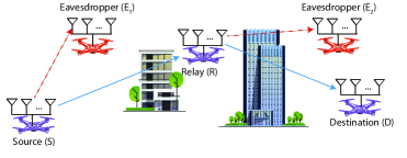
Figure 1: System model.

We consider a dual-hop UAV-based WCS consisting of a source node $(S)$ connected to a destination $(D)$ via a relay $(R)$ employing DF protocol. Two eavesdroppers, $E_{1}$ and $E_{2}$, try to intercept the legitimate messages broadcasted by $S$ and $R$, in the first and second time slots, respectively. We assume that the transmit nodes ($S$, $R$) are equipped with a single transmit antenna while all receiving nodes ($R,$ $D$, $E_{1},$ and $E_{2}$) are equipped with $N_{R},$ $N_{D},$ $N_{E_{1}},$ and $N_{E_{2}}$ receiving antennas, respectively. Lastly, due to the limited UAV transmit power and the significant distance between $S$ and $D$, we assume that there are no direct links from $S$ to $D$ and $E_{2}$. Without loss of generality, the received signals at $R$, $D,$ $E_{1},$ and $E_{2}$ are expressed as

$$y_{U}=\mathbf{h}_{SU}x+\mathbf{n}_{U},U\in\{R,E_{1}\},$$ (1)

$$y_{V}=\mathbf{h}_{RV}x^{\prime}+\mathbf{n}_{V},V\in\{D,E_{2}\},$$ (2)

where $x$ is the transmit signal, $x^{\prime}$ is the decoded and regenerated one by $R$, $\mathbf{n}_{U}$ and $\mathbf{n}_{V}$ are the additive white Gaussian noise (AWGN) realizations at either $R$, $D,$ $E_{1}$ or $E_{2}$’s antennas, which are independent and identically distributed (i.i.d) zero-mean complex Gaussian random variables (ZMCGRVs) with distribution $\mathcal{CN}\left(0,\sigma_{n_{Z}}^{2}\right)$, with $Z\in\left\{U,V\right\}$. Additionally,

$$\mathbf{h}_{SU}=\left[h_{SU}^{(1)},...,h_{SU}^{(N_{U})}\right]^{T}$$ (3)

and

$$\mathbf{h}_{RV}=\left[h_{RV}^{(1)},...,h_{RV}^{(N_{V})}\right]^{T}$$ (4)

are the $S$-$U$ and $R$-$V$ channel fading vector between $S/R$’s transmit antenna and $U/V$’s receive ones, whose elements are complex-valued i.i.d random variables with a fading envelope assumed to follow Nakagami-$m$ distribution with fading parameter $m_{XZ}$ and average fading power $\Omega_{XZ}=\mathbb{E}\left[\left|h_{XZ}^{(i)}\right|^{2}\right].$

Due to the UAV nodes’ mobility, the actual channel fading coefficients ($\mathbf{h}_{SU}$ and $\mathbf{h}_{RV}$) are different from the estimated one. Such a relationship can be expressed through the widely-known first-order autoregressive process, $AR(1)$, as follows [36, 20]

$$\mathbf{h}_{XZ}=\rho_{XZ}\overline{\mathbf{h}}_{XZ}+\sqrt{1-\rho_{XZ}^{2}}\mathbf{w}_{XZ},$$ (5)

where $\rho_{XZ}$ is the underlying correlation coefficient, with $XZ\in\left\{SR,\text{ }SE_{1},\text{ }RD,\text{ }RE_{2}\right\}$, $\overline{\mathbf{h}}_{XZ}$ is the exact outdated CSI vector, and $\mathbf{w}_{XZ}$ is the mobility noise vector whose entries are i.i.d ZMCGRVs with distribution $\mathcal{CN}\left(0,\sigma_{w_{XZ}}^{2}\right)$. On the other hand, the correlation coefficient $\rho_{XZ}$ is defined, according to the Jakes’ model, as [34, 36]

$$\rho_{XZ}=J_{0}\left(\frac{2\pi v_{XZ}f_{c}\tau}{c}\right),$$ (6)

which is a function of the two nodes’ relative speed $v_{XZ}$ along with the delay time $\tau$ between the CSI estimation and signal reception, and the carrier frequency $f_{c}.\$Moreover, in addition to the channel decorrelation over time, its estimation is also subject to the inherent noise in the receiver’s tracking loop. The final expression of the channel fading coefficient can be expressed as [36]

$$\mathbf{h}_{XZ}=\rho_{XZ}\underset{\overline{\mathbf{h}}_{XZ}}{\underbrace{\left(\mathbf{\hat{h}}_{XZ}+\mathbf{\varepsilon}_{XZ}\right)}}+\sqrt{1-\rho_{XZ}^{2}}\mathbf{w}_{XZ},$$ (7)

where $\mathbf{\hat{h}}_{XZ}$ is the estimated channel vector, and $\mathbf{\varepsilon}_{XZ}$ is the estimation noise vector with i.i.d ZMCGRVs entries with distribution $\mathcal{CN}\left(0,\sigma_{\varepsilon_{XZ}}^{2}\right)$.

Remark 1.

The channel’s mobility-dependent correlation coefficient $\left(\text{i.e., }\rho_{XZ}\right),$ given in (6), manifests the impact of nodes’ mobility on the time-varying statistical behavior of the channel. Such coefficient is expressed in terms of the nodes’ relative speed, carrier frequency, delay, and speed of light. A static scenario, i.e., $v_{XZ}=0$, corresponds to $\rho_{XZ}=1,$ which refers to a perfect correlation case. Likewise, at very high $v_{XZ}$ and/or $f_{c}$ and/or $\tau$, $\rho_{XZ}$ tends to 0, yielding severe channel time variations, in which the estimated CSI is completely uncorrelated with the actual one. Also, it worth mentioning that $J_{0}\left(x\right)$ in (6), with $x=\frac{2\pi v_{XZ}f_{c}\tau}{c},$ is a decreasing function of $v_{XZ}$ and/or $f_{c}$ and/or $\tau$ over $x\in\left[0,x_{0}\right],$ with $x_{0}=3.8317$ being the function’s minima that can be found numerically by retrieving the first zero of $\left(J_{0}\left(x\right)\right)^{\prime}$.

At the legitimate and wiretap nodes (i.e., $R$, $D,$ $E_{1}$, or $E_{2})$, the MRC receiver is used to combine the received signals copies on its various diversity branches. To this end, the combined signal at the output of the MRC receiver at such nodes can be formulated as

$$y_{Z}^{(MRC)} =\rho_{XZ}\mathbf{\phi}_{XZ}\mathbf{\hat{h}}_{XZ}u+\rho_{XZ}\mathbf{\phi}_{XZ}\mathbf{\varepsilon}_{XZ}u$$

$$+\mathbf{\phi}_{XZ}\sqrt{1-\rho_{XZ}^{2}}\mathbf{w}_{XZ}u+\mathbf{\phi}_{XZ}\mathbf{n}_{Z},$$ (8)

for $XZ\in\left\{SR,\text{ }RD,\text{ }SE_{1},\text{ }RE_{2}\right\}$, where

$$u=\left\{\begin{array}[]{l}x,\text{ if }Z\in\left\{R,E_{1}\right\}\\ x^{\prime},\text{ if }Z\in\left\{D,E_{2}\right\}\end{array}\right.,$$ (9)

and $\mathbf{\phi}_{XZ}=\frac{\left(\mathbf{\hat{h}}_{XZ}\right)^{H}}{\left\|\mathbf{\hat{h}}_{XZ}\right\|_{2}}$ denotes the MRC  beamforming vector. As a result, the corresponding instantaneous SNRs at the output of the receiving nodes’ combiners can be written using the following generalized form

$$\gamma_{XZ} = \frac{\rho_{XZ}^{2}P_{X}\left\|\mathbf{\hat{h}}_{XZ}\right\|_{2}^{2}}{P_{X}\left(\rho_{XZ}^{2}\sigma_{\varepsilon_{XZ}}^{2}+\left(1-\rho_{XZ}^{2}\right)\sigma_{w_{XZ}}^{2}\right)+\sigma_{n_{Z}}^{2}},$$ (10)

$$= \sum\limits_{i=1}^{N_{Z}}\gamma_{XZ}^{(i)},$$

where $P_{X}$ is the transmit power of node $X$, and

$$\gamma_{XZ}^{(i)}=\frac{P_{X}\rho_{XZ}^{2}\left|\hat{h}_{XZ}^{(i)}\right|^{2}}{P_{X}\left(\rho_{XZ}^{2}\sigma_{\varepsilon_{XZ}}^{2}+\left(1-\rho_{XZ}^{2}\right)\sigma_{w_{XZ}}^{2}\right)+\sigma_{n_{Z}}^{2}}$$ (11)

denotes the instantaneous SNR at the $i$th branch, with an average value given as

$$\Upsilon_{XZ}=\frac{\rho_{XZ}^{2}\delta_{XZ}}{\frac{\delta_{XZ}}{\Omega_{XZ}}\left(\rho_{XZ}^{2}\sigma_{\varepsilon_{XZ}}^{2}+\left(1-\rho_{XZ}^{2}\right)\sigma_{w_{XZ}}^{2}\right)+1},$$ (12)

with $\delta_{XZ}=\frac{P_{X}\Omega_{XZ}}{\sigma_{n_{Z}}^{2}}.$

Remark 2.

1. By differentiating the average SNR per branch in (12) with respect to $\rho_{XZ}$, it yields

   $$\frac{\partial\Upsilon_{XZ}}{\partial\rho_{XZ}}=\frac{2\rho_{XZ}\delta_{XZ}\left[1+\frac{\delta_{XZ}\sigma_{w_{XZ}}^{2}}{\Omega_{XZ}}\right]}{\left(\frac{\delta_{XZ}}{\Omega_{XZ}}\left(\rho_{XZ}^{2}\sigma_{\varepsilon_{XZ}}^{2}+\left(1-\rho_{XZ}^{2}\right)\sigma_{w_{XZ}}^{2}\right)+1\right)^{2}},$$ (13)

   which is strictly positive. Henceforth, we can conclude that the effective per-branch average SNR is an increasing function of the correlation coefficient $\rho_{XZ}.$

2. On the other hand, one can note from (12) that at higher average SNR values (i.e., $\delta_{XZ}\rightarrow\infty$), the effective average SNR per branch $\left(\text{i.e., }\Upsilon_{XZ}\right)$ converges to the following ceiling value

   $$\Upsilon_{XZ}^{\left(\infty\right)}=\frac{\rho_{XZ}^{2}\Omega_{XZ}}{\left(\rho_{XZ}^{2}\sigma_{\varepsilon_{XZ}}^{2}+\left(1-\rho_{XZ}^{2}\right)\sigma_{w_{XZ}}^{2}\right)}.$$ (14)

   The above upper bound of $\Upsilon_{XZ}$ leads to saturation floors in the system’s IP at high $\delta_{XZ}$ values, within which the IP will be depending essentially on $\rho_{XZ}^{2},$ $\sigma_{\varepsilon_{XZ}}^{2},$ and $\sigma_{w_{XZ}}^{2}$ values. As a consequence, we can conclude that the impact of nodes mobility jointly with estimation imperfections can lead to remarkable secrecy performance limitations which need to be considered in the design of such systems.

III Statistical Properties

In this section, statistical properties such as the probability density function (PDF) and the cumulative distribution function (CDF) of the per-hop SNR are presented.

From (10), one can infer that the instantaneous SNRs are proportional to the sum of Gamma-distributed squared fading envelopes at each branch of the receiver. To this end, the respective PDF and CDF of such instantaneous SNRs can be written as [17]

$$f_{\gamma_{XZ}}\left(y\right)=\frac{\left(\frac{m_{XZ}}{\Upsilon_{XZ}}\right)^{m_{XZ}N_{Z}}}{\Gamma\left(m_{XZ}N_{Z}\right)}y^{m_{XZ}N_{Z}-1}\exp\left(-\frac{m_{XZ}}{\Upsilon_{XZ}}y\right),$$ (15)

and

$$F_{\gamma_{SE_{1}}}\left(y\right)=\frac{\gamma_{\text{inc}}\left(m_{XZ}N_{Z},\frac{m_{XZ}}{\Upsilon_{XZ}}y\right)}{\Gamma\left(m_{XZ}N_{Z}\right)},$$ (16)

respectively.

IV Secrecy Analysis

In this section, exact closed-form and asymptotic expressions of the IP are derived, in terms of the main setup parameters.

The IP metric is defined as the probability that the secrecy capacity, which is the difference between the capacity of the legitimate channels and that of the eavesdropping ones, is less than or equal to zero. Mathematically, it is defined as [50]

$$P_{int} =\Pr\left(C_{s}\leq 0\right)$$

$$=1-\Pr\left(C_{s}>0\right),$$ (17)

where

$$C_{s}=\min\left(C_{s}^{(SR)},C_{s,eq}^{(RD)}\right),$$ (18)

$$C_{s}^{(SR)}=\log_{2}\left(\frac{1+\gamma_{SR}}{1+\gamma_{SE_{1}}}\right),$$ (19)

and

$$C_{S,eq}^{(RD)}=\min\left(C_{s}^{(SRD)},C_{s}^{(RD)}\right),$$ (20)

refer to the end-to-end, first hop, and second hops’ secrecy capacities, respectively, by assuming DF relaying protocol, with

$$C_{s}^{(SRD)} = \log_{2}\left(\frac{1+\gamma_{SR}}{1+\gamma_{RE_{2}}}\right),$$ (21)

$$C_{s}^{(RD)} = \log_{2}\left(\frac{1+\gamma_{RD}}{1+\gamma_{RE_{2}}}\right).$$ (22)

To this end, the total secrecy capacity in (18) can be formulated as follows

$$C_{s}=\min\left(C_{s}^{(SR)},C_{s}^{(RD)},C_{s}^{(SRD)}\right).$$ (23)

Leveraging the probability theory, (17) becomes

$$P_{int} =1-\Pr\left(C_{s}>0,\gamma_{SR}>\gamma_{th}\right)$$

$$-\Pr\left(C_{s}>0,\gamma_{SR}<\gamma_{th}\right),$$ (24)

where $\gamma_{th}$ is a decoding threshold SNR, below which the decoding process can not be performed at the relay.

When $\gamma_{SR}<\gamma_{th},$ the relay fails at decoding the information message. Therefore, no signal will be transmitted to $D$ as well as the eavesdropper $E_{2}.$ Hence, we have $\gamma_{RD}=\gamma_{RE_{2}}=0$, which yields from (20), (21), and (22) that $C_{s,eq}^{(RD)}\leq 0,$ and consequently, it yields from (18) that $C_{s}\leq 0$ and $\Pr\left(C_{s}>0,\gamma_{SR}<\gamma_{th}\right)=0.$ As a result, the overall IP expression in (24) reduces to

$$P_{int}=1-\Pr\left(C_{s}>0,\gamma_{SR}>\gamma_{th}\right).$$ (25)

Remark 3.

1. From (23), it can be noticed that the system’s secrecy capacity is the minimum of three elementary secrecy capacities, namely the first hop’s one; i.e., $C_{s}^{(SR)}$; the second’s; i.e., $C_{s}^{(RD)}$; and a cross-term one; i.e., $C_{s}^{(SRD)}$; which involves the first hop’s legitimate SNR along with the second hop’s wiretap one. Indeed, the higher are these three terms, the greater the overall system’s secrecy capacity. Notably, one can note from (19), (21), and (22) that such elementary secrecy capacities, and consequently the overall one in (23), increase with the rise of the legitimate instantaneous per-hop SNRs, i.e., $\gamma_{SR}$ and $\gamma_{RD}$ (better system secrecy), and decrease versus the wiretap ones, i.e., $\gamma_{SE_{1}}$ and $\gamma_{RE_{2}}$ (worse system secrecy). Thus, the IP, given by (17) is a decreasing function of $\gamma_{SR}$ and $\gamma_{RD}$, and increasing with respect to $\gamma_{SE_{1}}$ and $\gamma_{RE_{2}}.$

2. The secrecy capacities in (19), (21), and (22) can be written in a generalized form as

   $$C_{s}^{\left(\xi\right)}=\log_{2}\left(\frac{1+\varrho_{l}g_{l}}{1+\varrho_{w}g_{w}}\right),$$ (26)

   with $\varrho_{x}=\frac{\Upsilon_{x}}{\Omega_{x}},x\in\left\{l,w\right\},$

   $$\left(\xi,l,w\right)\in\left\{\begin{array}[]{l}\left(SR,SR,SE_{1}\right),\\ \left(SRD,SR,RE_{2}\right),\\ \left(RD,RD,RE_{2}\right)\end{array}\right\},$$ (27)

   and

   $$g_{x}=\sum\limits_{i=1}^{N^{(x)}}\left|h_{x}^{(i)}\right|^{2},$$ (28)

   with $N^{(x)}=\left\{\begin{array}[]{l}N_{R},\left(x=l=SR\right)\\ N_{D},\left(x=l=RD\right)\\ N_{E_{1}},\left(x=w=SE_{1}\right)\\ N_{E_{2}},\left(x=w=RE_{2}\right)\end{array}\right..$

   Thus, as mentioned in Remark 3.1, a secure system from the PLS perspective corresponds to a higher secrecy capacity. To this end, it can be intuitively noticed from (26) and (28) that the higher $\varrho_{l}$ and/or the number of legitimate nodes’ antennas (i.e., $N_{R},N_{D}$), the greater is $C_{s}^{\left(\xi\right)}$. Likewise, this latter drops by increasing $\varrho_{w}$ and/or $N_{E_{1}},$ $N_{E_{2}}$. Therefore, to gain more insights, we inspect the behavior of $C_{s}^{\left(\xi\right)}$, for equal average SNRs, i.e., $\varrho_{l}=\varrho_{w}=\varrho$, and number of antennas, i.e., $N^{(l)}=N^{(w)}$, by differentiating $C_{s}^{\left(\xi\right)}$ with respect to $\varrho$ as

   $$\frac{\partial C_{s}^{\left(\xi\right)}}{\partial\varrho}=\frac{g_{l}-g_{w}}{\left(1+\varrho g_{l}\right)\left(1+\varrho g_{w}\right)}.$$ (29)

   One can note from (29) that $C_{s}^{\left(\xi\right)}$ is an increasing function of $\varrho$ iff $g_{l}-g_{w}>0.$ Notably, as this last-mentioned quantity is random, we are interested then into analyzing the probability$:\ \Pr\left[g_{l}-g_{w}>0\right].$ Hence, it yields

   $$\mathcal{Y} = \Pr\left[g_{l}-g_{w}>0\right],$$ (30)

   $$= \int_{0}^{\infty}F_{g_{w}}\left(y\right)f_{g_{l}}\left(y\right)dy,$$

   where $F_{g_{w}}\left(.\right)$ and $f_{g_{l}}\left(.\right)$ are given, respectively, as follows

   $$F_{g_{w}}\left(y\right)=\frac{\gamma_{\text{inc}}\left(m_{w}N^{\left(w\right)},\frac{m_{w}}{\Omega_{w}}y\right)}{\Gamma\left(m_{w}N^{\left(w\right)}\right)},$$ (31)

   $$f_{g_{l}}\left(y\right)=\frac{\left(\frac{m_{l}}{\Omega_{l}}\right)^{m_{l}N^{(l)}}}{\Gamma\left(m_{l}N^{\left(l\right)}\right)}y^{m_{l}N^{\left(l\right)}-1}\exp\left(-\frac{m_{l}}{\Omega_{l}}y\right).$$ (32)

   Thus, it produces

   $$\mathcal{Y} \mathcal{=}\frac{\left(\frac{m_{l}}{\Omega_{l}}\right)^{m_{l}N^{\left(l\right)}}}{\Gamma\left(m_{l}N^{\left(l\right)}\right)\Gamma\left(m_{w}N^{\left(w\right)}\right)}\int_{0}^{\infty}\gamma_{\text{inc}}\left(m_{w}N^{(w)},\frac{m_{w}}{\Omega_{w}}y\right)$$

   $$\times y^{m_{l}N^{\left(l\right)}-1}\exp\left(-\frac{m_{l}}{\Omega_{l}}y\right)dy.$$ (33)

   Through the use of [54, Eq. (6.455.1)] , one obtains (34) given at the top of the next page.

   Figs. 2 and 3 present the plot of (34) versus $m_{l}$ and $m_{w}$ (Fig. 2), and $\Omega_{l}$ and $\Omega_{w}$ (Fig. 3), with $N^{(l)}=N^{(w)}=3$. It can be noted from Fig. 2 that $\mathcal{Y}$ slightly increases versus $m_{l}$ and decreases versus $m_{w}.$ Essentially, for equal number of antennas, this probability does not exceed $56\%$ for $m_{x}\leq 10$. Nevertheless, as seen from Fig. 3, $\mathcal{Y}$ (i.e., the probability that $C_{s}^{\left(\xi\right)}$ is increasing vs $\varrho$) surpasses $99$% for $\Omega_{l}\geq 4\Omega_{w}.$

   $$\mathcal{Y}\mathcal{=}\frac{\left(\frac{m_{l}}{\Omega_{l}}\right)^{m_{l}N^{\left(l\right)}}\left(\frac{m_{w}}{\Omega_{w}}\right)^{m_{w}N^{\left(w\right)}}\Gamma\left(m_{l}N^{\left(l\right)}+m_{w}N^{\left(w\right)}\right)}{\Gamma\left(m_{l}N^{\left(l\right)}\right)\Gamma\left(m_{w}N^{\left(w\right)}+1\right)\left(\frac{m_{w}}{\Omega_{w}}+\frac{m_{l}}{\Omega_{l}}\right)^{m_{l}N^{\left(l\right)}+m_{w}N^{\left(w\right)}}}\text{ }_{2}F_{1}\left(1,m_{l}N^{\left(l\right)}+m_{w}N^{\left(w\right)};m_{w}N^{\left(w\right)}+1;\frac{\frac{m_{w}}{\Omega_{w}}}{\frac{m_{w}}{\Omega_{w}}+\frac{m_{l}}{\Omega_{l}}}\right).$$ (34)

   
   

   

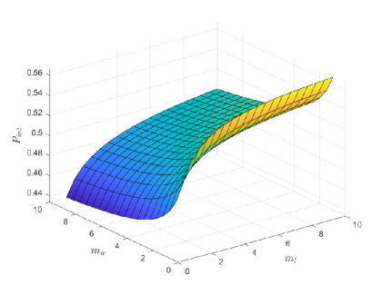
   Figure 2: IP versus $m_{l}$ and $m_{w}$, for $\Omega_{l}=\Omega_{w}=2.5$, $N^{(l)}=N^{(w)}=3$.

   

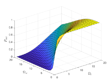
   Figure 3: IP versus $\Omega_{l}$ and $\Omega_{w}$, for $m_{l}=m_{w}=2$, $N^{(l)}=N^{(w)}=3$.

IV-A Exact Analysis

Proposition 1.

The IP of the considered dual-hop UAV-based WCS is given in closed-form expression as

$$P_{int} =1-\frac{\left(\frac{m_{SR}}{\Upsilon_{SR}}\right)^{m_{SR}N_{R}}\left(\frac{m_{RE_{2}}}{\Upsilon_{RE_{2}}}\right)^{m_{RE_{2}}N_{E_{2}}}}{\left(m_{SR}N_{R}-1\right)!\left(m_{RE_{2}}N_{E_{2}}-1\right)!}$$

$$\times\sum_{l=0}^{m_{RD}N_{D}-1}\frac{\left(m_{RE_{2}}N_{E_{2}}+l-1\right)!\left(\frac{m_{RD}}{\Upsilon_{RD}}\right)^{l}}{l!\left[\frac{m_{RE_{2}}}{\Upsilon_{RE_{2}}}+\frac{m_{RD}}{\Upsilon_{RD}}\right]^{m_{RE_{2}}N_{E_{2}}+l}}\sum_{i=1}^{4}\mathcal{I}^{(i)},$$ (35)

where

$$\mathcal{I}^{(1)}=\frac{\Gamma_{\text{inc}}\left(m_{SR}N_{R},\frac{m_{SR}}{\Upsilon_{SR}}\gamma_{th}\right)}{\left(\frac{m_{SR}}{\Upsilon_{SR}}\right)^{m_{SR}N_{R}}},$$ (36)

$$\mathcal{I}^{(2)} =-\sum_{n=0}^{m_{SE_{1}}N_{E_{1}}-1}\frac{\left(\frac{m_{SE_{1}}}{\Upsilon_{SE_{1}}}\right)^{n}}{\left[\frac{m_{SR}}{\Upsilon_{SR}}+\frac{m_{SE_{1}}}{\Upsilon_{SE_{1}}}\right]^{m_{SR}N_{R}+n}n!}$$

$$\times\Gamma_{\text{inc}}\left(m_{SR}N_{R}+n,\left[\frac{m_{SR}}{\Upsilon_{SR}}+\frac{m_{SE_{1}}}{\Upsilon_{SE_{1}}}\right]\gamma_{th}\right),$$ (37)

$$\mathcal{I}^{(3)} =-\sum_{p=0}^{m_{RE_{2}}N_{E_{2}}+l-1}\frac{\left(\frac{m_{RE_{2}}}{\Upsilon_{RE_{2}}}+\frac{m_{RD}}{\Upsilon_{RD}}\right)^{p}}{p!}$$

$$\times\frac{\Gamma_{\text{inc}}\left(m_{SR}N_{R}+p,\Delta\gamma_{th}\right)}{\Delta^{m_{SR}N_{R}+p}},$$ (38)

$$\mathcal{I}^{(4)} =\sum_{n=0}^{m_{SE_{1}}N_{E_{1}}-1}\left(\sum_{p=0}^{m_{RE_{2}}N_{E_{2}}+l-1}\frac{\left(\frac{m_{RE_{2}}}{\Upsilon_{RE_{2}}}+\frac{m_{RD}}{\Upsilon_{RD}}\right)^{p}}{n!p!}\right.$$

$$\times\left.\frac{\Gamma_{\text{inc}}\left(m_{SR}N_{R}+n+p,\Psi\gamma_{th}\right)\left(\frac{m_{SE_{1}}}{\Upsilon_{SE_{1}}}\right)^{n}}{\Psi^{m_{SR}N_{R}+n+p}}\right),$$ (39)

$\Delta=\frac{m_{RE_{2}}}{\Upsilon_{RE_{2}}}+\frac{m_{RD}}{\Upsilon_{RD}}+\frac{m_{SR}}{\Upsilon_{SR}},$ and $\Psi=\Delta+\frac{m_{SE_{1}}}{\Upsilon_{SE_{1}}}.$

Proof.

The proof is provided in Appendix A. ∎

Remark 4.

1. The IP closed-form expression, given by (35)-(39) is formulated in terms of finite summations, upper-incomplete and complete Gamma functions, and exponential terms. All the system and channel parameters are involved in such functions, such as Nakagami-$m$ fading parameter $\left(m_{XZ}\right)$, the threshold SNR $\gamma_{th}$, and effective average SNRs $\left(\Upsilon_{XZ}\right).$ These latter are essentially expressed, as shown in (12), in terms of the respective mobility-dependent correlation coefficients $\left(\rho_{XZ}\right)$, computed based on UAVs’ relative speed, carrier frequency, and delay, average fading power $\left(\Omega_{XZ}\right)$, and noise powers due to the CSI estimation errors and mobility $\left(\sigma_{\varepsilon_{XZ}}^{2},\sigma_{w_{XZ}}^{2}\right)$. Of note, the aforementioned functions are already implemented in almost all computational software (e.g., MATLAB, MATHEMATICA), which can provide insightful observations on the impact of the system parameters on the overall secrecy performance.

2. One can obviously note that at lower threshold SNR values; i.e., $\gamma_{th}\rightarrow 0$; the terms (36)-(39), leveraging $\Gamma_{\text{inc}}\left(a,0\right)=\Gamma\left(a\right),$ reduce to

   $$\mathcal{V}^{(1)}=\frac{\left(m_{SR}N_{R}-1\right)!}{\left(\frac{m_{SR}}{\Upsilon_{SR}}\right)^{m_{SR}N_{R}}},$$ (40)

   $$\mathcal{V}^{(2)}=-\sum_{n=0}^{m_{SE_{1}}N_{E_{1}}-1}\frac{\left(\frac{m_{SE_{1}}}{\Upsilon_{SE_{1}}}\right)^{n}\left(m_{SR}N_{R}+n-1\right)!}{n!\left[\frac{m_{SR}}{\Upsilon_{SR}}+\frac{m_{SE_{1}}}{\Upsilon_{SE_{1}}}\right]^{m_{SR}N_{R}+n}},$$ (41)

   $$\mathcal{V}_{l}^{(3)} =-\sum_{p=0}^{m_{RE_{2}}N_{E_{2}}+l-1}\frac{\left(m_{SR}N_{R}+p-1\right)!}{p!}$$

   $$\times\frac{\left(\frac{m_{RE_{2}}}{\Upsilon_{RE_{2}}}+\frac{m_{RD}}{\Upsilon_{RD}}\right)^{p}}{\Delta^{m_{SR}N_{R}+p}},$$ (42)

   and

   $$\mathcal{V}_{l}^{(4)} =\sum_{n=0}^{m_{SE_{1}}N_{E_{1}}-1}\sum_{p=0}^{m_{RE_{2}}N_{E_{2}}+l-1}\frac{\left(m_{SR}N_{R}+n+p-1\right)!}{\Psi^{m_{SR}N_{R}+n+p}}$$

   $$\times\frac{\left(\frac{m_{SE_{1}}}{\Upsilon_{SE_{1}}}\right)^{n}\left(\frac{m_{RE_{2}}}{\Upsilon_{RE_{2}}}+\frac{m_{RD}}{\Upsilon_{RD}}\right)^{p}}{n!p!},$$ (43)

   which are independent of $\gamma_{th}$. Henceforth, in this regime, the system’s IP is not improved regardless of the decrease in $\gamma_{th}$ (i.e., increasing the decoding probability at the relay), as the IP depends exclusively on the per-node number of antennas, links’ fading parameters, and average SNRs.

3. On the other hand, by making use of [54, Eq. (8.350.4)], i.e., $\Gamma_{\text{inc}}\left(a,\infty\right)=0$ $\forall a>0$, the terms (36)-(39) vanish for high $\gamma_{th}$ values (i.e., $\gamma_{th}\rightarrow\infty$). Henceforth, the IP, given by (35), reaches one. In fact, the greater $\gamma_{th}$, the lower is the probability of successful decoding at the relay. As such, the relay fails at relaying the information signal to $D$, which results in zero capacity/SNR of the second hop.

IV-B Asymptotic Analysis

In this subsection, asymptotic expressions for the system’s IP are derived at high legitimate links’ average SNR values. Two scenarios are investigated, namely (i) moving nodes with imperfect channel estimation, and (ii) static nodes with perfect CSI at the receiver.

IV-B1 Scenario I (Moving UAVs with Imperfect CSI)

In this scenario, when the average SNRs $\delta_{SR}$ and $\delta_{RD}$ become high (i.e., $\delta_{SR},$ $\delta_{RD}\rightarrow\infty$), their corresponding effective ones, given by (12), reduce to

$$\Xi_{XZ}\sim\frac{\rho_{XZ}^{2}\Omega_{XZ}}{\rho_{XZ}^{2}\sigma_{\varepsilon_{XZ}}^{2}+\left(1-\rho_{XZ}^{2}\right)\sigma_{w_{XZ}}^{2}},XZ\in\left\{SR,RD\right\}.$$ (44)

As a consequence, by substituting $\Upsilon_{XZ}$ $\left(XZ\in\left\{SR,RD\right\}\right)$ in (35)-(39) by $\Xi_{XZ}$, given by the above equation, the system’s IP in such a particular case can be expressed as

$$P_{int}^{\left(\infty,1\right)} \sim 1-\frac{\left(\frac{m_{SR}}{\Xi_{SR}}\right)^{m_{SR}N_{R}}\left(\frac{m_{RE_{2}}}{\Upsilon_{RE_{2}}}\right)^{m_{RE_{2}}N_{E_{2}}}}{\left(m_{SR}N_{R}-1\right)!\left(m_{RE_{2}}N_{E_{2}}-1\right)!}$$

$$\times \sum_{l=0}^{m_{RD}N_{D}-1}\frac{\left(m_{RE_{2}}N_{E_{2}}+l-1\right)!\left(\frac{m_{RD}}{\Xi_{RD}}\right)^{l}}{l!\left[\frac{m_{RE_{2}}}{\Upsilon_{RE_{2}}}+\frac{m_{RD}}{\Xi_{RD}}\right]^{m_{RE_{2}}N_{E_{2}}+l}}\sum_{i=1}^{4}\mathcal{H}^{(i)},$$ (45)

where

$$\mathcal{H}^{(1)}=\frac{\Gamma_{\text{inc}}\left(m_{SR}N_{R},\frac{m_{SR}}{\Xi_{SR}}\gamma_{th}\right)}{\left(\frac{m_{SR}}{\Xi_{SR}}\right)^{m_{SR}N_{R}}},$$ (46)

$$\mathcal{H}^{(2)} =-\sum_{n=0}^{m_{SE_{1}}N_{E_{1}}-1}\frac{\left(\frac{m_{SE_{1}}}{\Upsilon_{SE_{1}}}\right)^{n}}{n!}$$

$$\times\frac{\Gamma_{\text{inc}}\left(m_{SR}N_{R}+n,\left[\frac{m_{SR}}{\Xi_{SR}}+\frac{m_{SE_{1}}}{\Upsilon_{SE_{1}}}\right]\gamma_{th}\right)}{\left[\frac{m_{SR}}{\Xi_{SR}}+\frac{m_{SE_{1}}}{\Upsilon_{SE_{1}}}\right]^{m_{SR}N_{R}+n}},$$ (47)

$$\mathcal{H}^{(3)} =-\sum_{p=0}^{m_{RE_{2}}N_{E_{2}}+l-1}\frac{\left(\frac{m_{RE_{2}}}{\Upsilon_{RE_{2}}}+\frac{m_{RD}}{\Xi_{RD}}\right)^{p}}{p!}$$

$$\times\frac{\Gamma_{\text{inc}}\left(m_{SR}N_{R}+p,\mathcal{Q}\gamma_{th}\right)}{\mathcal{Q}^{m_{SR}N_{R}+p}},$$ (48)

$$\mathcal{H}^{(4)} =\sum_{p=0}^{m_{RE_{2}}N_{E_{2}}+l-1}\left(\sum_{n=0}^{m_{SE_{1}}N_{E_{1}}-1}\frac{\left(\frac{m_{RE_{2}}}{\Upsilon_{RE_{2}}}+\frac{m_{RD}}{\Xi_{RD}}\right)^{p}}{p!}\right.$$

$$\times\left.\frac{\left(\frac{m_{SE_{1}}}{\Upsilon_{SE_{1}}}\right)^{n}\Gamma_{\text{inc}}\left(m_{SR}N_{R}+p+n,\mathcal{S}\gamma_{th}\right)}{n!\mathcal{S}^{m_{SR}N_{R}+p+n}}\right),$$ (49)

with $\mathcal{Q}=\frac{m_{RE_{2}}}{\Upsilon_{RE_{2}}}+\frac{m_{RD}}{\Xi_{RD}}+\frac{m_{SR}}{\Xi_{SR}},$ and $\mathcal{S}=\mathcal{Q}+\frac{m_{SE_{1}}}{\Upsilon_{SE_{1}}}.$

Remark 5.

The IP’s asymptotic expansion for Scenario I, given by (45)-(49), is independent from $\delta_{SR}$ and $\delta_{RD}$. For fixed values of the remainder of system and channel parameters, the IP exhibits asymptotic floors at the high SNR regime. Hence, the system’s secrecy is not improved further regardless of the increase in $\delta_{SR}$ and/or $\delta_{RD}.$ Consequently, the secrecy diversity order in this scenario is equal to zero. Therefore, the system’s IP in the high SNR regime, for this scenario, depends exclusively on the remainder of system parameters, namely the number of antennas $\left(N_{Z},\text{ }Z\in\{R,D,E_{1},E_{2}\}\right),$ fading parameters $\left(m_{XZ},\text{ }XZ\in\{SR,RD,SE_{1},RE_{2}\}\right)$, wiretap links’ effective average SNRs $\left(\Upsilon_{SE_{1}},\text{ }\Upsilon_{RE_{2}}\right),$ per-hop mobility-dependent correlation coefficients $\rho_{XZ},$ and the noise powers due to channel estimation errors and mobility $\left(\sigma_{\varepsilon_{XZ}}^{2},\text{ }\sigma_{w_{XZ}}^{2}\right).$

IV-B2 Scenario II (Static Nodes with Perfect CSI)

In this scenario, leveraging Remark 1, the mobility-dependent correlation coefficients, given in (6), equals 1. Furthermore, under perfect channel estimation, we have $\sigma_{\varepsilon_{XZ}}^{2}=0.$ To this end, the per-hop effective average SNR in (12) reduces to $\delta_{XZ}.$

Proposition 2.

At high average SNRs $\left(\text{i.e., }\delta_{SR}=\delta_{RD}=\delta\rightarrow\infty\right)$, the IP of the considered dual-hop UAV-based WCS can be asymptotically expanded, for Scenario II, as

$$P_{int}^{\left(\infty,2\right)}\sim G_{c}\delta^{-G_{d}},$$ (50)

where

$$G_{c}=\left\{\begin{array}[]{l}\mathcal{R},m_{SR}N_{R}>m_{RD}N_{D}\\ \mathcal{T}_{1}+\mathcal{T}_{2}-\mathcal{T}_{3},m_{SR}N_{R}<m_{RD}N_{D}\\ \mathcal{R}+\mathcal{T}_{1}+\mathcal{T}_{2}-\mathcal{T}_{3},m_{SR}N_{R}=m_{RD}N_{D}\end{array}\right.,$$ (51)

with

$$\mathcal{R=}\left(\frac{m_{RD}\delta_{RE_{2}}}{m_{RE_{2}}}\right)^{m_{RD}N_{D}}\frac{\left(m_{RE_{2}}N_{E_{2}}+m_{RD}N_{D}-1\right)!}{\left(m_{RE_{2}}N_{E_{2}}-1\right)!\left(m_{RD}N_{D}\right)!},$$ (52)

$$\mathcal{T}_{1} =\frac{\left(m_{SR}\gamma_{th}\right)^{m_{{}_{SR}}N_{R}}\gamma_{inc}\left(m_{RE_{2}}N_{E_{2}},\frac{m_{RE_{2}}}{\delta_{RE_{2}}}\gamma_{th}\right)}{\left(m_{SR}N_{R}\right)!\left(m_{RE_{2}}N_{E_{2}}-1\right)!}$$

$$\times\frac{\gamma_{inc}\left(m_{SE_{1}}N_{E_{1}},\frac{m_{SE_{1}}}{\delta_{SE_{1}}}\gamma_{th}\right)}{\left(m_{SE_{1}}N_{E_{1}}-1\right)!},$$ (53)

$$\mathcal{T}_{2} =\frac{m_{SR}^{m_{SR}N_{R}}\left(\mathcal{F}_{SE_{1}}+\mathcal{F}_{RE_{2}}\right)}{\left(m_{SR}N_{R}\right)!},$$ (54)

$$\mathcal{T}_{3} =\frac{m_{SR}^{m_{SR}N_{R}}\left(\mathcal{G}_{S,E_{1},R,E_{2}}+\mathcal{G}_{R,E_{2},S,E_{1}}\right)}{\left(m_{SR}N_{R}\right)!},$$ (55)

$$\mathcal{F}_{x,y}=\frac{\left(\frac{\delta_{xy}}{m_{xy}}\right)^{m_{SR}N_{R}}\Gamma_{\text{inc}}\left(m_{xy}N_{y}+m_{SR}N_{R},\frac{m_{xy}}{\delta_{xy}}\gamma_{th}\right)}{\left(m_{xy}N_{y}-1\right)!},$$ (56)

$$\mathcal{G}_{x,y,z,t} =\frac{\left(\frac{m_{xy}}{\delta_{xy}}\right)^{m_{xy}N_{y}}}{\left(m_{xy}N_{y}-1\right)!}\sum_{n=0}^{m_{zt}N_{t}-1}\frac{\left(\frac{m_{zt}}{\delta_{zt}}\right)^{n}}{n!}$$

$$\times\frac{\Gamma_{\text{inc}}\left(m_{xy}N_{y}+m_{SR}N_{R}+n,\left(\frac{m_{xy}}{\delta_{xy}}+\frac{m_{zt}}{\delta_{zt}}\right)\gamma_{th}\right)}{\left(\frac{m_{xy}}{\delta_{xy}}+\frac{m_{zt}}{\delta_{zt}}\right)^{n+m_{xy}N_{y}+m_{SR}N_{R}}},$$ (57)

and

$$G_{d}=\min\left(m_{SR}N_{R},m_{RD}N_{D}\right),$$ (58)

are the respective secrecy coding gain and diversity order, respectively.

Proof.

The proof is provided in Appendix B. ∎

Remark 6.

Equations (50)-(58) provide an asymptotic expression of the IP in the high SNR regime for Scenario II, written in terms of finite summations, Gamma and lower/upper incomplete Gamma functions, and exponential terms. Such expression can give insightful observations of the impact of the setup parameters on the security level in the high SNR regime. Interestingly, the achievable secrecy diversity order for this scenario depends exclusively on the legitimate links’ fading parameters and the number of antennas; i.e., $G_{d}=\min\left(m_{SR}N_{R},m_{RD}N_{D}\right)$.

V Numerical Results

In this section, numerical results for the secrecy performance of the considered dual-hop UAV-based WCS are presented. The IP metric is evaluated for several configurations of system and channel parameters. Unless otherwise stated, the default values of the system parameters are listed in Table I. Moreover, without loss of generality, the mobility-dependent noise power can be computed as follows: $\sigma_{w_{XZ}}^{2}=\Omega_{XZ}+\sigma_{\varepsilon_{XZ}}^{2}$ [20]. It is worth mentioning that throughout the numerical results, the relative speed between two nodes $X$ and $Z$ can refer to two UAVs moving either in the same direction, i.e., $v_{XZ}=\left|v_{Z}-v_{X}\right|$, or in opposite ones, i.e., $v_{XZ}=v_{X}+v_{Z}$. Also, we use the notation $\delta=\delta_{SR}=\delta_{RD},$ when the IP is plotted against $\delta_{SR}$, with $\delta_{RD}=\delta_{SR}$. Lastly, Monte Carlo simulations were performed by generating $9\times 10^{6}$ Gamma-distributed RVs, referring to the per-hop SNRs, with PDF and CDF given by (15) and (16), respectively.

TABLE I: Simulation parameters’ values.

Parameter	Value
$f_{c}$	$2.4$ GHz
$\tau$	1 ms
$v_{X};X\in\left\{S,R,D,E_{1},E_{2}\right\}$	25 Km/h
$m_{XZ};XZ\in\left\{SR,RD,SE_{1},RE_{2}\right\}$	2
$\delta_{SR}=\delta_{RD}=\delta$	$30$ dB
$\delta_{SE_{1}}=\delta_{RE_{2}}$	$10$ dB
$\sigma_{\varepsilon_{XZ}}^{2};XZ\in\left\{SR,RD,SE_{1},RE_{2}\right\}$	$0.1$
$\Omega_{XZ}$	2
$N_{R},N_{D}$	4
$N_{E_{1}},N_{E_{2}}$	2
$\gamma_{th}$	3

V-A Effect of the Fading Severity Parameters and Number of Antennas

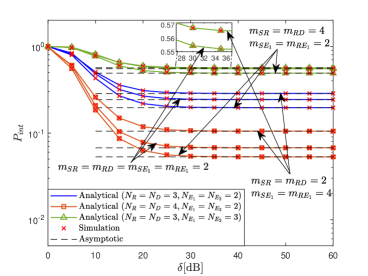
Figure 4: IP versus $\delta$ for various $\left(m_{XZ},N_{Z}\right)_{XZ\in\left\{SR,RD,SE_{1},RE_{2}\right\}}$ values.

Fig. 4 presents the system’s IP versus the average legitimate SNR, i.e., $\delta_{SR}=\delta_{RD}=\delta$, for several combinations of the fading severity parameter and number of antennas. One can note from this figure that the analytical curves, plotted using (35), match their simulations counterpart, which corroborates the accuracy of the derived IP expression. Furthermore, at high SNR, the IP justifies with the asymptotic floors, plotted using (45)-(49), where the secrecy diversity order equals zero as pointed out in Remark 2.2 and Remark 5. On the other hand, one can note that the system’s secrecy improves by increasing either the legitimate link’s fading severity parameters and/or the number of receive antennas (i.e., higher $m_{SR},$ $m_{RD}$ and/or $N_{R},$ $N_{D})$. It is important to note that when the eavesdropping links are enhanced, either in terms of the number of antennas onboard and/or the fading severity parameter, the system’s secrecy deteriorates, where the IP can reach $50\%\$ for $m_{XZ}=2$ $\left(XZ\in\left\{SR,\text{ }RD,\text{ }RE_{1},\text{ }RE_{2}\right\}\right)$ and $N_{Z}=3.$

V-B Effect of the CSI Imperfection Level

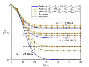
Figure 5: IP versus $\delta$ for various $\left(\sigma_{\varepsilon_{XZ}}^{2},v_{XZ}\right)_{XZ\in\left\{SR,\text{ }RD,\text{ }SE_{1},\text{ }RE_{2}\right\}}$ values.

In Fig. 5, the IP is depicted vs $\delta_{SR}=\delta_{RD}=\delta$ for numerous combinations of CSI estimation noise power $\left(\sigma_{\varepsilon_{XZ}}^{2}\right)$ and nodes relative speed values. We can notice that CSI estimation noise power $\left(\text{i.e., }\sigma_{\varepsilon_{XZ}}^{2}\right)$ impacts negatively the system’s IP. Specifically, three cases are considered in this figure: (i) Case 1:$\ \ \left(\sigma_{\varepsilon_{SR}}^{2}=\sigma_{\varepsilon_{RD}}^{2}=0.02,\text{ }\sigma_{\varepsilon_{SE_{1}}}^{2}=\sigma_{\varepsilon_{RE_{2}}}^{2}=0.09\right)$; i.e., both legitimate links’ have less estimation error noise compared to their wiretap counterpart; (ii) Case 2: $\left(\sigma_{\varepsilon_{SR}}^{2}=0.02,\text{ }\sigma_{\varepsilon_{RD}}^{2}=\sigma_{\varepsilon_{SE_{1}}}^{2}=\sigma_{\varepsilon_{RE_{2}}}^{2}=0.09\right)$; i.e., estimation error at the $R$-$D$ link increases; and (iii) Case 3: $\left(\sigma_{\varepsilon_{RD}}^{2}=0.02,\text{ }\sigma_{\varepsilon_{SR}}^{2}=\sigma_{\varepsilon_{SE_{1}}}^{2}=\sigma_{\varepsilon_{RE_{2}}}^{2}=0.09\right)$; i.e., estimation error at the $S$-$R$ link increases. It is obvious that Case 1 exhibits the best secrecy performance when both legitimate links experience less CSI estimation noise compared to their malign counterpart. However, we can note that Case 2 manifests a slightly improved performance compared to Case 3. That is, increasing CSI imperfection power on the first legitimate hop has a more negative impact on the system’s secrecy compared to the case when the CSI imperfection at the second hop is magnified. Lastly, it can be ascertained as well that, for fixed $\sigma_{\varepsilon_{XZ}}^{2}$, $\left(\text{i.e., }\sigma_{\varepsilon_{SR}}^{2}=0.02;\sigma_{\varepsilon_{RD}}^{2}=\sigma_{\varepsilon_{SE_{1}}}^{2}=\sigma_{\varepsilon_{RE_{2}}}^{2}=0.09\right),$ the system’s secrecy degrades when the nodes’ relative speed increases, where it can reach $17.24\%$ at $v_{XZ}=70$ km/h.

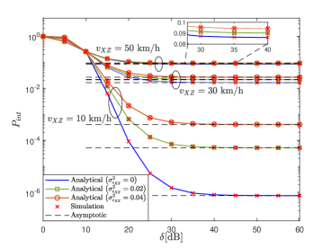
Figure 6: IP versus $\delta$ for various $\left(\sigma_{\varepsilon_{XZ}}^{2},v_{XZ}\right)_{XZ\in\left\{SR,\text{ }RD,\text{ }SE_{1},\text{ }RE_{2}\right\}}$ values.

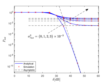
Figure 7: IP versus $\delta$ for various $\left(\sigma_{\varepsilon_{XZ}}^{2}\right)_{XZ\in\left\{SR,\text{ }RD,\text{ }SE_{1},\text{ }RE_{2}\right\}}$ values and static nodes.

To emphasize Fig. 5 results, Fig. 6 represent the IP behavior versus $\delta$ for equal $\sigma_{\varepsilon_{XZ}}^{2}$ on all links, and various speed values. Notably, for perfect CSI (solid lines), the IP exhibits a remarkable increase by a factor of $10^{4}$ when the relative speed of nodes increases from 10 to 30 km/h. The degradation, however, is less significant with respect to the speed, for the remaining two levels of CSI imperfection. Moreover, at 50 km/h, there is almost no noticeable impact of the CSI estimation noise level on the performance.

From another front, Fig. 7 shows the IP performance for static nodes, with $\delta_{SE_{1}}=\delta_{RE_{2}}=30$ dB, and considering various levels of CSI imperfections $\left(\sigma_{\varepsilon_{XZ}}^{2}\right)$. The results emphatically highlight the IP linear drop for the ideal case $\left(\text{i.e., }v_{XZ}=\sigma_{\varepsilon_{XZ}}^{2}=0\right),$ where the analytical IP curve matches its asymptotic counterpart, plotted from (50), at high $\delta$ values. In such a case, $\delta\rightarrow\infty\Longleftrightarrow\Upsilon_{SR},$ $\Upsilon_{RD}\rightarrow\infty$. Thus, the achievable diversity order for this case equals $\min\left(m_{SR}N_{R},\text{ }m_{RD}N_{D}\right)$ as discussed in Remark 6; i.e., the achievable diversity order equals $8$ for this ideal setup $\left(m_{SR}=m_{RD}=2,\text{ }N_{R}=N_{D}=4\right).$ On the other hand, one can note in parallel that even slight increases in $\sigma_{\varepsilon_{XZ}}^{2}$ can drastically impact the performance, where the IP exhibits a 15 dB loss at $IP\approx 3\times 10^{-3}$ when going from the ideal case to $\sigma_{\varepsilon_{XZ}}^{2}=10^{-3}.$ Also, one can observe that the IP for the imperfect CSI case reaches asymptotic floors at higher $\delta$ values, where the corresponding legitimate average SNR, given by (12), reaches a ceiling value, as detailed in Remark 2.2. Thus, the secrecy diversity order in such a scenario equals zero, as pointed out in Remark 5.

V-C Effect of the Legitimate/Wiretap Average SNRs

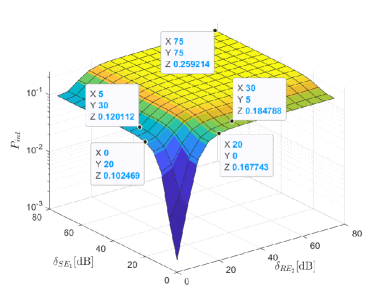
Figure 8: IP versus $\delta_{SE_{1}}$ and $\delta_{RE_{2}}$.

Fig. 8 provides the IP plot in three dimensions versus the average SNR of the wiretap links, i.e.,  $\delta_{SE_{1}}$ and $\delta_{RE_{2}}$, with $\delta_{SR}=\delta_{RD}=40$ dB. Expectedly, the IP is an increasing function of both malign channels’ SNRs. Notably, at low SNR values, we notice that the IP does not exhibit symmetric behavior for both eavesdropper’s SNRs. Importantly, at low and mid SNR values, and $\beta>\alpha$ $\left(\alpha,\text{ }\beta\in\mathbb{R}_{+}^{\ast}\right)$, the IP evaluated at $\delta_{SE_{1}}=\alpha$ and $\delta_{RE_{2}}=\beta$ exceeds the one evaluated at $\delta_{SE_{1}}=\beta$ and $\delta_{RE_{2}}=\alpha$; e.g., IP$=16.77\%$ for $\left(\delta_{SE_{1}},\text{ }\delta_{RE_{2}}\right)=\left(0,20\right)$ dB, while IP$=10.24\%$ for $\left(\delta_{SE_{1}},\text{ }\delta_{RE_{2}}\right)=\left(20,0\right)$ dB. Therefore, deteriorating the link quality of the second malign user can provide a better secrecy performance than worsening the first one’s channel. Lastly, the IP manifests a saturation regime at high $\left(\delta_{SE_{1}},\delta_{RE_{2}}\right)$ values, where the IP reaches $26\%$. As detailed in Remark 2.2, for fixed $\Upsilon_{SR},\Upsilon_{RD}$ values, the average wiretap SNRs $\left(\text{i.e., }\Upsilon_{SE_{1}},\text{ }\Upsilon_{RE_{2}}\right)$ exhibit a ceiling value at higher $\delta_{SE_{1}}$ and $\delta_{RE_{2}}.$ Therefore, the IP in this regime depends on the remainder of system parameters (i.e., legitimate SRNRs values, number of antennas, fading parameters, correlation coefficients, and CSI imperfection level).

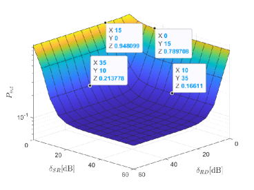
Figure 9: IP versus $\delta_{SR}$ and $\delta_{RD}.$

Fig. 9 depicts the secrecy performance in three dimensions versus the average SNR of both hops, i.e., $\delta_{SR}$ and $\delta_{RD}$. Expectedly, the IP is a decreasing function of both $\delta_{SR}$ and $\delta_{RD},$ where it reaches a ceiling value as pointed out in Remark 2.2 and Remark 5. Also, in a similar fashion to Fig. 8, the IP does not exhibit symmetric behavior vs $\delta_{SR}$ and $\delta_{RD},$ particularly at low SNR values. For instance, $P_{int}=0.1661$ for $\left(\delta_{SR},\delta_{RD}\right)=\left(35,10\right)$ dB, while $P_{int}=0.2138$ for $\left(\delta_{SR},\delta_{RD}\right)=\left(10,35\right)$ dB. Thus, the IP can be improved by strengthening the first hop’s channel quality.

V-D Effect of the Decoding Threshold SNR

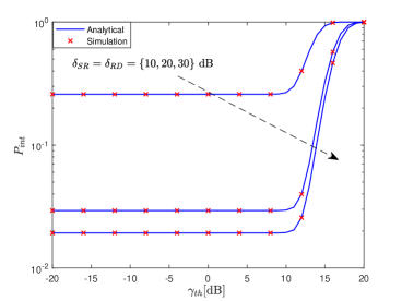
Figure 10: IP versus $\gamma_{th}$ for various $\left(\delta_{XZ}\right)_{XZ\in\left\{SR,RD,SE_{1},RE_{2}\right\}}$ values.

In Fig. 10, the system secrecy performance is shown vs $\gamma_{th}$, with $v_{XZ}=20$ km/h $\left(XZ\in\left\{SR,SE_{1},RD,RE_{2}\right\}\right).$ It can be ascertained that the IP reaches error floors at low $\gamma_{th}$ values, while at higher $\gamma_{th}$, it reaches unit. Indeed, as discussed in Remark 4.2, the terms $\mathcal{I}^{(i)}$ of (35), given by (36)-(39), reduce to (40)-(43), which are independent of $\gamma_{th}$. Furthermore, as highlighted in Remark 4.3, the IP was shown to converge to one at high $\gamma_{th}$, i.e., the higher $\gamma_{th}$, the lower is the decoding success probability at $R$. Henceforth, this results in a zero capacity of the second hop, leading to a second hop’s secrecy capacity equal to zero, according to (22). Thus, relying on the IP definition in (17)-(23), the IP will be evidently equal to 1.

V-E Effect of the Carrier Frequency and Delay

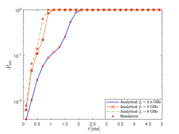
Figure 11: IP versus $\tau$ for three main carrier frequency $f_{c}$ values.

Fig. 11 presents the system’s IP with respect to the CSI estimation time delay $\tau,$ for three main carrier frequency values, i.e., $f_{c}=2.4$, $5,$ and $6$ GHz, with $\delta_{SR}=\delta_{RD}=40$ dB. It is obvious from the figure that the higher the delay and/or the carrier frequency, the worse is the IP performance. Indeed, as discuss in Remark 1, $\rho_{XZ}$, given by (6), is decreasing over the interval $\left[0,\frac{2\pi v_{XZ}f_{c}\tau_{0}}{c}=3.8317\right],$ where $\tau_{0}\$equals $5.5,$ $2.6,$ and $2.2$ ms for $f_{c}=2.4,$ $5,$ and $6$ GHz, respectively. Notably, the IP reaches one at $\tau=2.1,$ $1.1,$ and $0.9$ ms, for $f_{c}=2.4,$ $5,$ and $6$ GHz, respectively. Indeed, as mentioned above, the correlation coefficient decreases over the intervals $\left[0,5.5\right]$ ms, $\left[0,2.6\right]$ ms, and $\left[0,2.2\right]$ ms for the three considered frequencies in ascending order. Thus, capitalizing on Remark 2.1, it yields a decrease as well in the per-hop average SNR, given by (12), over these aforementioned intervals, leading to an increase in the system’s IP. Importantly, we can observe that the IP remains constant at one, although the correlation coefficient reincreases (i.e., reincrease of $\Upsilon_{SR}$ and $\Upsilon_{RD}$) when $\tau_{0}>2.6$ ms and $\tau_{0}>2.2$ ms, for $f_{c}=$ $5,$ and $6$ GHz, respectively.

V-F Effect of Nodes’ Speed

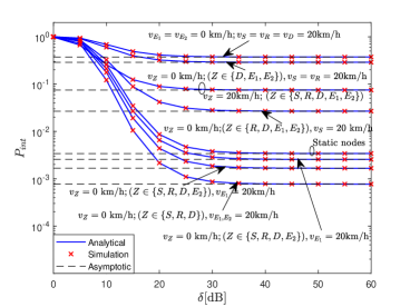
Figure 12: IP versus $\delta$ for various values of $\left(v_{S},v_{R},v_{D},v_{E_{1}},v_{E_{2}}\right)$.

Fig. 12 presents the IP behavior vs $\delta$, for various nodes’ mobility scenarios. We assume that $v_{XZ}=v_{X}+v_{Z}$ $\left(XZ\in\left\{SR,\text{ }RD,\text{ }SE_{1},\text{ }RE_{2}\right\}\right),$ which corresponds to the case of two moving UAVs in opposite directions. It can be noted that the worst performance corresponds to the case of moving legitimate nodes and static wiretap ones. The lesser the number of moving benign nodes, the better is the performance. Indeed, as emphasized in Remark 1, and for $v_{XZ}\in\left[0,\frac{3.8317c}{2\pi f_{c}\tau_{0}}\right]$, the greater the relative speed $v_{XZ}$, the lower is the correlation coefficient. Thus, the respective average SNR decreases, as shown in Remark 2.1. We can note as well that the best performance corresponds to the case of moving wiretappers and static legitimate nodes.

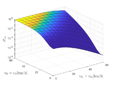
Figure 13: IP versus $v_{R}$ and $v_{E_{1}}.$

Fig. 13 shows the IP evolution in three dimensions, versus $v_{R}$ and $v_{E_{1}}.$ We set $v_{S}=0$, $v_{D}=v_{R},$ and $v_{E_{2}}=v_{E_{1}}.$ It can be noted that, for fixed legitimate nodes’ speed, the IP manifests a decreasing behavior vs the wiretappers’ speed. In fact, as discussed in Remark 1, the greater the speed, the lower the correlation coefficient, leading to a decrease in the average SNR. Likewise, the IP deteriorates for fixed malign nodes speed and increasing velocity of the benign ones.

VI Conclusion

In this paper, the secrecy performance of a dual-hop UAV-based WCS system was analyzed. Particularly, a DF relay handles the information signal from a source to a destination, under the presence of two malicious nodes attempting independently to overhear the $S$-$R$ and $R$-$D$ hops. Transmitters ($S,R$) are assumed to be equipped with a single transmit antenna, while receivers ($R,D,E_{1},E_{2}$) perform maximal-ratio combining using their multiple receive antennas. Due to nodes’ mobility and channel estimation imperfections at the receivers, the CSI is subject to time selectivity and estimation errors. The per-hop instantaneous SNRs were expressed in terms of the mobility-dependent correlation coefficient and CSI estimation errors, by using the $AR\left(1\right)$ model along with Gaussian estimation errors. Using per-hop SNR statistics, exact closed-form and asymptotic expressions for the IP metric were derived. In particular, asymptotic expressions were retrieved for two scenarios: (i) mobile nodes with imperfect CSI (general case), and (ii) static nodes with perfect CSI estimation (ideal case). It was shown that the IP admits a zero diversity order for the first scenario, due to the presence of a ceiling value of the average SNR per branch. However, the IP decreases linearly versus the average SNR in the second one, with an achievable diversity order dependant on the fading parameters and number of antennas of the legitimate links/nodes. Furthermore, for static nodes, the system can be castigated by a $15$ dB secrecy loss at IP$=3\times 10^{-3},$ when the CSI imperfection power raises from $0$ to $10^{-3}$. Finally, we showed that the higher the legitimate nodes’ speed and/or carrier frequency and/or delay time and/or relay’s decoding threshold SNR, the worse is the system’s secrecy.

Appendix A: Proof of Proposition 1

The IP of a dual-hop DF-based WCS, subject to the presence of an eavesdropper per hop is given as [50, Eq. (33)]

$$P_{int}=1-\int_{y=\gamma_{th}}^{\infty}f_{\gamma_{SR}}\left(y\right)F_{\gamma_{SE_{1}}}\left(y\right)\mathcal{J}(y)dy,$$ (59)

where

$$\mathcal{J}(y)=\int_{z=0}^{y}f_{\gamma_{RE_{2}}}\left(z\right)F_{\gamma_{RD}}^{\left(c\right)}\left(z\right)dz,$$ (60)

and $F_{.}^{\left(c\right)}\left(.\right)=1-F_{.}\left(.\right)$ accounts for the complementary CDF. By plugging the PDF and CDF from (15) and (16), with $XZ=RE_{2}$ and $XZ=RD,$ respectively, into (60), it yields (61)-(63) at the top of the next page, where Step (a) holds by involving the expressions (15) and (16) into (60), while Step (b) is reached by using the finite-sum representation of $\Gamma_{\text{inc}}\left(.,.\right)$ [54, Eq. (8.352.2)] along with [54, Eq. (8.339.1)], assuming $m_{XZ}\in\mathbb{N}^{\ast}$. Finally, using [54, Eq. (3.381.1)], Step (c) is attained.

By involving (15) and (16) with $XZ=SR$ and $XZ=SE_{1},$ respectively, along with (63) into (59), using [54, Eq. (8.339.1)] for $m_{XZ}\in\mathbb{N}^{\ast}$, and performing some algebraic manipulations, one obtains (64), with $\mathcal{I}$ and $\left(\mathcal{I}^{(i)}\right)_{1\leq i\leq 4},$ given in (65)-(71), defined in the next page, where $\Delta$ and $\Psi$ are defined in the proposition. Step (a) is $\mathcal{I}$’s definition, Step (b) yields from using the finite-sum representation of $\gamma_{\text{inc}}\left(.,.\right)$ [54, Eq. (8.352.1)], while Step (c) and (68)-(71) are obtained by expanding Step (b). Finally, armed by [54, Eq. (3.381.3)] to solve (68)-(71), (36)-(39) of Proposition 1 are obtained. This concludes the proposition’s proof.

$$\mathcal{J}(y) \overset{(a)}{=}\frac{\left(\frac{m_{RE_{2}}}{\Upsilon_{RE_{2}}}\right)^{m_{RE_{2}}N_{E_{2}}}}{\Gamma\left(m_{RE_{2}}N_{E_{2}}\right)\Gamma\left(m_{RD}N_{D}\right)}\int_{z=0}^{y}z^{m_{RE_{2}}N_{E_{2}}-1}\exp\left(-\frac{m_{RE_{2}}}{\Upsilon_{RE_{2}}}z\right)\Gamma_{inc}\left(m_{RD}N_{D},\frac{m_{RD}}{\Upsilon_{RD}}z\right)dz.$$ (61)

$$\overset{(b)}{=}\frac{\left(\frac{m_{RE_{2}}}{\Upsilon_{RE_{2}}}\right)^{m_{RE_{2}}N_{E_{2}}}}{\left(m_{RE_{2}}N_{E_{2}}-1\right)!}\sum_{l=0}^{m_{RD}N_{D}-1}\frac{\left(\frac{m_{RD}}{\Upsilon_{RD}}\right)^{l}}{l!}\int_{z=0}^{y}z^{m_{RE_{2}}N_{E_{2}}+l-1}\exp\left(-\left[\frac{m_{RE_{2}}}{\Upsilon_{RE_{2}}}+\frac{m_{RD}}{\Upsilon_{RD}}\right]z\right)dz.$$ (62)

$$\overset{(c)}{=}\frac{\left(\frac{m_{RE_{2}}}{\Upsilon_{RE_{2}}}\right)^{m_{RE_{2}}N_{E_{2}}}}{\left(m_{RE_{2}}N_{E_{2}}-1\right)!}\sum_{l=0}^{m_{RD}N_{D}-1}\frac{\left(\frac{m_{RD}}{\Upsilon_{RD}}\right)^{l}\gamma_{\text{inc}}\left(m_{RE_{2}}N_{E_{2}}+l,\left[\frac{m_{RE_{2}}}{\Upsilon_{RE_{2}}}+\frac{m_{RD}}{\Upsilon_{RD}}\right]y\right)}{l!\left[\frac{m_{RE_{2}}}{\Upsilon_{RE_{2}}}+\frac{m_{RD}}{\Upsilon_{RD}}\right]^{l+m_{RE_{2}}N_{E_{2}}}}.$$ (63)

$$P_{int} =1-\frac{\left(\frac{m_{SR}}{\Upsilon_{SR}}\right)^{m_{SR}N_{R}}\left(\frac{m_{RE_{2}}}{\Upsilon_{RE_{2}}}\right)^{m_{RE_{2}}N_{E_{2}}}}{\left(m_{SR}N_{R}-1\right)!\left(m_{RE_{2}}N_{E_{2}}-1\right)!}\sum_{l=0}^{m_{RD}N_{D}-1}\frac{\left(m_{RE_{2}}N_{E_{2}}+l-1\right)!\left(\frac{m_{RD}}{\Upsilon_{RD}}\right)^{l}}{l!\left[\frac{m_{RE_{2}}}{\Upsilon_{RE_{2}}}+\frac{m_{RD}}{\Upsilon_{RD}}\right]^{m_{RE_{2}}N_{E_{2}}+l}}$$

$$\times\underset{\triangleq\mathcal{I}}{\underbrace{\left[\int_{y=\gamma_{th}}^{\infty}y^{m_{SR}N_{R}-1}\exp\left(-\frac{m_{SR}}{\Upsilon_{SR}}y\right)\frac{\gamma_{\text{inc}}\left(m_{RE_{2}}N_{E_{2}}+l,\left[\frac{m_{RE_{2}}}{\Upsilon_{RE_{2}}}+\frac{m_{RD}}{\Upsilon_{RD}}\right]y\right)\gamma_{\text{inc}}\left(m_{SE_{1}}N_{E_{1}},\frac{m_{SE_{1}}}{\Upsilon_{SE_{1}}}y\right)}{\left(m_{RE_{2}}N_{E_{2}}+l-1\right)!\left(m_{SE_{1}}N_{E_{1}}-1\right)!}dy\right]}}.$$ (64)

$$\mathcal{I} \overset{(a)}{=}\int_{y=\gamma_{th}}^{\infty}y^{m_{SR}N_{R}-1}\exp\left(-\frac{m_{SR}}{\Upsilon_{SR}}y\right)\frac{\gamma_{\text{inc}}\left(m_{RE_{2}}N_{E_{2}}+l,\left[\frac{m_{RE_{2}}}{\Upsilon_{RE_{2}}}+\frac{m_{RD}}{\Upsilon_{RD}}\right]y\right)\gamma_{\text{inc}}\left(m_{SE_{1}}N_{E_{1}},\frac{m_{SE_{1}}}{\Upsilon_{SE_{1}}}y\right)}{\left(m_{RE_{2}}N_{E_{2}}+l-1\right)!\left(m_{SE_{1}}N_{E_{1}}-1\right)!}dy.$$ (65)

$$\overset{(b)}{=}\int_{y=\gamma_{th}}^{\infty}y^{m_{SR}N_{R}-1}\exp\left(-\frac{m_{SR}}{\Upsilon_{SR}}y\right)\left[1-\exp\left(-\frac{m_{SE_{1}}}{\Upsilon_{SE_{1}}}y\right)\sum_{n=0}^{m_{SE_{1}}N_{E_{1}}-1}\frac{\left(\frac{m_{SE_{1}}}{\Upsilon_{SE_{1}}}y\right)^{n}}{n!}\right]$$

$$\times\left[1-\exp\left(-\left[\frac{m_{RE_{2}}}{\Upsilon_{RE_{2}}}+\frac{m_{RD}}{\Upsilon_{RD}}\right]y\right)\sum_{p=0}^{m_{RE_{2}}N_{E_{2}}+l-1}\frac{\left(\left[\frac{m_{RE_{2}}}{\Upsilon_{RE_{2}}}+\frac{m_{RD}}{\Upsilon_{RD}}\right]y\right)^{p}}{p!}\right]dy.$$ (66)

$$\overset{(c)}{=}\sum\limits_{i=1}^{4}\mathcal{I}^{(i)}.$$ (67)

$$\mathcal{I}^{(1)} =\int_{y=\gamma_{th}}^{\infty}y^{m_{SR}N_{R}-1}\exp\left(-\frac{m_{SR}}{\Upsilon_{SR}}y\right)dy.$$ (68)

$$\mathcal{I}^{(2)} =-\sum_{n=0}^{m_{SE_{1}}N_{E_{1}}-1}\frac{\left(\frac{m_{SE_{1}}}{\Upsilon_{SE_{1}}}\right)^{n}}{n!}\int_{y=\gamma_{th}}^{\infty}y^{m_{SR}N_{R}+n-1}\exp\left(-\left[\frac{m_{SR}}{\Upsilon_{SR}}+\frac{m_{SE_{1}}}{\Upsilon_{SE_{1}}}\right]y\right)dy.$$ (69)

$$\mathcal{I}^{(3)} =-\sum_{p=0}^{m_{RE_{2}}N_{E_{2}}+l-1}\frac{\left(\frac{m_{RE_{2}}}{\Upsilon_{RE_{2}}}+\frac{m_{RD}}{\Upsilon_{RD}}\right)^{p}}{p!}\int_{y=\gamma_{th}}^{\infty}y^{m_{SR}N_{R}+p-1}\exp\left(-\Delta y\right)dy.$$ (70)

$$\mathcal{I}^{(4)} =\sum_{n=0}^{m_{SE_{1}}N_{E_{1}}-1}\frac{\left(\frac{m_{SE_{1}}}{\Upsilon_{SE_{1}}}\right)^{n}}{n!}\sum_{p=0}^{m_{RE_{2}}N_{E_{2}}+l-1}\frac{\left(\frac{m_{RE_{2}}}{\Upsilon_{RE_{2}}}+\frac{m_{RD}}{\Upsilon_{RD}}\right)^{p}}{p!}\int_{y=\gamma_{th}}^{\infty}y^{m_{SR}N_{R}+n+p-1}\exp\left(-\Psi y\right)dy.$$ (71)

Appendix B: Proof of Proposition 2

In Scenario II, as mentioned before Proposition 2, the effective average SNRs $\Upsilon_{XZ}$ in (12) reduce to $\delta_{XZ}$ $\left(\text{i.e., }\Upsilon_{XZ}=\delta_{XZ}\right)$. At the high SNR regime $\left(\text{i.e., }\delta_{SR}=\delta_{RD}=\delta\rightarrow\infty\right),$ and relying on the IP definition in (59), we can asymptotically expand it as follows

$$P_{int}^{\left(\infty,2\right)}=1-\int_{y=\gamma_{th}}^{\infty}f_{\gamma_{SR}}^{\left(\infty\right)}\left(y\right)F_{\gamma_{SE_{1}}}\left(y\right)\mathcal{J}^{\left(\infty\right)}(y)dy,$$ (72)

with

$$\mathcal{J}^{\left(\infty\right)}(y)=\int_{z=0}^{y}f_{\gamma_{RE_{2}}}\left(z\right)F_{\gamma_{RD}}^{\left(c,\infty\right)}\left(z\right)dz,$$ (73)

$f_{\gamma_{SR}}^{\left(\infty\right)}\left(y\right)$, and $F_{\gamma_{RD}}^{\left(c,\infty\right)}\left(z\right)$ being the asymptotic representations of $\mathcal{J}(y)$,$\ f_{\gamma_{SR}}\left(y\right)$, and $F_{\gamma_{RD}}^{\left(c\right)}\left(z\right)$ at the high SNR values, respectively. In such a regime, using the limit of the exponential function, i.e., $\lim\limits_{x\rightarrow 0}\exp\left(-x\right)=1$, along with the incomplete Gamma expansion [55, Eq. (06.06.06.0001.02)], the PDF and CDF expressions in (15) and (16) can be expanded asymptotically as

$$f_{\gamma_{XZ}}^{\left(\infty\right)}\left(y\right)=\frac{\left(\frac{m_{XZ}}{\delta_{XZ}}\right)^{m_{XZ}N_{Z}}}{\Gamma\left(m_{XZ}N_{Z}\right)}y^{m_{XZ}N_{Z}-1},$$ (74)

and

$$F_{\gamma_{XZ}}^{\left(\infty\right)}\left(y\right)=\frac{\left(\frac{m_{XZ}}{\delta_{XZ}}y\right)^{m_{XZ}N_{Z}}}{\Gamma\left(m_{XZ}N_{Z}+1\right)},$$ (75)

$$\mathcal{J}^{\left(\infty\right)}(y) \overset{(a)}{=}\frac{\left(\frac{m_{RE_{2}}}{\delta_{RE_{2}}}\right)^{m_{RE_{2}}N_{E_{2}}}}{\left(m_{RE_{2}}N_{E_{2}}-1\right)!}\int_{z=0}^{y}z^{m_{RE_{2}}N_{E_{2}}-1}\exp\left(-\frac{m_{RE_{2}}}{\delta_{RE_{2}}}z\right)\left[1-\frac{\left(\frac{m_{RD}}{\delta}z\right)^{m_{RD}N_{D}}}{\left(m_{RD}N_{D}\right)!}\right]dz.$$ (76)

$$\overset{(b)}{=}\frac{\gamma_{inc}\left(m_{RE_{2}}N_{E_{2}},\frac{m_{RE_{2}}}{\delta_{RE_{2}}}y\right)}{\left(m_{RE_{2}}N_{E_{2}}-1\right)!}-\frac{\left(\frac{m_{RD}}{\delta}\right)^{m_{RD}N_{D}}\left(\frac{m_{RE_{2}}}{\delta_{RE_{2}}}\right)^{m_{RE_{2}}N_{E_{2}}}\gamma_{inc}\left(m_{RE_{2}}N_{E_{2}}+m_{RD}N_{D},\frac{m_{RE_{2}}}{\delta_{RE_{2}}}y\right)}{\left(\frac{m_{RE_{2}}}{\delta_{RE_{2}}}\right)^{m_{RE_{2}}N_{E_{2}}+m_{RD}N_{D}}\left(m_{RE_{2}}N_{E_{2}}-1\right)!\left(m_{RD}N_{D}\right)!}.$$ (77)

respectively. Given that $F_{\gamma_{XZ}}^{\left(c,\infty\right)}\left(y\right)=1-F_{\gamma_{XZ}}^{\left(\infty\right)}\left(y\right)$, by plugging (15) with $\left(XZ=RE_{2},\Upsilon_{RE_{2}}=\delta_{RE_{2}}\right)$ and (75) with $\left(XZ=RD,\delta_{RD}=\delta\right)$ into (73), respectively, and using [54, Eq. (8.339.1)] for $m_{XZ}\in\mathbb{N}^{\ast}$, one obtains (76)-(77), shown at the top of the page after next, where Step (a) is the definition of $\mathcal{J}^{\left(\infty\right)}(y),$ while Step (b) is attained using [54, Eq. (3.381.1)]. By involving (16) with $\left(XZ=SE_{1},\Upsilon_{SE_{1}}=\delta_{SE_{1}}\right)$, (74) with $\left(XZ=SR,\delta_{SR}=\delta\right)$, and (77) into (72), it yields the asymptotic expansion of the IP at the high SNR as

$$P_{int}^{\left(\infty,2\right)} \overset{(a)}{\sim}1-\int_{y=\gamma_{th}}^{\infty}f_{\gamma_{SR}}^{\left(\infty\right)}\left(y\right)F_{\gamma_{SE_{1}}}\left(y\right)\mathcal{J}^{\left(\infty\right)}(y)dy$$ (78)

$${\overset{(b)}{\sim}}1-\left[F_{\gamma_{SR}}^{\left(\infty\right)}\left(y\right)F_{\gamma_{SE_{1}}}\left(y\right)\mathcal{J}^{\left(\infty\right)}(y)\right]_{\gamma_{th}}^{\infty}$$

$$+\int_{y=\gamma_{th}}^{\infty}F_{\gamma_{SR}}^{\left(\infty\right)}\left(y\right)\left[F_{\gamma_{SE_{1}}}\left(y\right)\mathcal{J}^{\left(\infty\right)}(y)\right]^{\prime}dy$$ (79)

$${\overset{(c)}{\sim}}\mathcal{U}_{1}+\mathcal{U}_{2}+\mathcal{U}_{3}+\mathcal{U}_{4},$$ (80)

$$\mathcal{U}_{1} =\frac{\left(\frac{m_{RD}}{\delta}\right)^{m_{RD}N_{D}}\left(\frac{m_{RE_{2}}}{\delta_{RE_{2}}}\right)^{m_{RE_{2}}N_{E_{2}}}\left(m_{RE_{2}}N_{E_{2}}+m_{RD}N_{D}-1\right)!}{\left(\frac{m_{RE_{2}}}{\delta_{RE_{2}}}\right)^{m_{RE_{2}}N_{E_{2}}+m_{RD}N_{D}}\left(m_{RE_{2}}N_{E_{2}}-1\right)!\left(m_{RD}N_{D}\right)!}.$$ (81)

$$\mathcal{U}_{2} =\left[\frac{\gamma_{inc}\left(m_{RE_{2}}N_{E_{2}},\frac{m_{RE_{2}}}{\delta_{RE_{2}}}\gamma_{th}\right)}{\left(m_{RE_{2}}N_{E_{2}}-1\right)!}-\frac{\left(\frac{m_{RD}}{\delta}\right)^{m_{RD}N_{D}}\left(\frac{m_{RE_{2}}}{\delta_{RE_{2}}}\right)^{m_{RE_{2}}N_{E_{2}}}\gamma_{inc}\left(m_{RE_{2}}N_{E_{2}}+m_{RD}N_{D},\frac{m_{RE_{2}}}{\delta_{RE_{2}}}\gamma_{th}\right)}{\left(\frac{m_{RE_{2}}}{\delta_{RE_{2}}}\right)^{m_{RE_{2}}N_{E_{2}}+m_{RD}N_{D}}\left(m_{RE_{2}}N_{E_{2}}-1\right)!\left(m_{RD}N_{D}\right)!}\right]$$

$$\times\frac{\gamma_{inc}\left(m_{SE_{1}}N_{E_{1}},\frac{m_{SE_{1}}}{\delta_{SE_{1}}}\gamma_{th}\right)\left(\frac{m_{SR}}{\delta}\gamma_{th}\right)^{m_{{}_{SR}}N_{R}}}{\left(m_{SE_{1}}N_{E_{1}}-1\right)!\left(m_{SR}N_{R}\right)!}.$$ (82)

$$\mathcal{U}_{3} \overset{(a)}{=}\int_{y=\gamma_{th}}^{\infty}F_{\gamma_{SR}}^{\left(\infty\right)}\left(y\right)f_{\gamma_{SE_{1}}}\left(y\right)\mathcal{J}^{\left(\infty\right)}(y)dy.$$ (83)

$$\overset{(b)}{=}\frac{\left(\frac{m_{SE_{1}}}{\delta_{SE_{1}}}\right)^{m_{SE_{1}}N_{E_{1}}}\left(\frac{m_{SR}}{\delta}\right)^{m_{SR}N_{R}}}{\left(m_{SR}N_{R}\right)!\left(m_{SE_{1}}N_{E_{1}}-1\right)!}\int_{y=\gamma_{th}}^{\infty}y^{m_{SE_{1}}N_{E_{1}}+m_{SR}N_{R}-1}\exp\left(-\frac{m_{SE_{1}}}{\delta_{SE_{1}}}z\right)$$

$$\times\left[\frac{\gamma_{inc}\left(m_{RE_{2}}N_{E_{2}},\frac{m_{RE_{2}}}{\delta_{RE_{2}}}y\right)}{\left(m_{RE_{2}}N_{E_{2}}-1\right)!}-\frac{\left(\frac{m_{RD}}{\delta}\right)^{m_{RD}N_{D}}\left(\frac{m_{RE_{2}}}{\delta_{RE_{2}}}\right)^{m_{RE_{2}}N_{E_{2}}}}{\left(\frac{m_{RE_{2}}}{\delta_{RE_{2}}}\right)^{m_{RE_{2}}N_{E_{2}}+m_{RD}N_{D}}}\frac{\gamma_{inc}\left(m_{RE_{2}}N_{E_{2}}+m_{RD}N_{D},\frac{m_{RE_{2}}}{\delta_{RE_{2}}}y\right)}{\left(m_{RE_{2}}N_{E_{2}}-1\right)!\left(m_{RD}N_{D}\right)!}\right]dy.$$ (84)

$$\mathcal{U}_{4} \overset{(a)}{=}\int_{y=\gamma_{th}}^{\infty}F_{\gamma_{SR}}^{\left(\infty\right)}\left(y\right)F_{\gamma_{SE_{1}}}\left(y\right)\left[\mathcal{J}^{\left(\infty\right)}(y)\right]^{\prime}dy.$$ (85)

$$\overset{(b)}{=}\frac{\left(\frac{m_{SR}}{\delta}\right)^{m_{SR}N_{R}}}{\left(m_{SR}N_{R}\right)!\left(m_{SE_{1}}N_{E_{1}}-1\right)!}\int_{y=\gamma_{th}}^{\infty}y^{m_{SR}N_{R}}\gamma_{inc}\left(m_{SE_{1}}N_{E_{1}},\frac{m_{SE_{1}}}{\delta_{SE_{1}}}y\right)$$

$$\times\left[\begin{array}[]{c}\frac{\exp\left(-\frac{m_{RE_{2}}}{\delta_{RE_{2}}}y\right)\left(\frac{m_{RE_{2}}}{\delta_{RE_{2}}}\right)^{m_{RE_{2}}N_{E_{2}}}y^{m_{RE_{2}}N_{E_{2}}-1}}{\left(m_{RE_{2}}N_{E_{2}}-1\right)!}-\frac{\left(\frac{m_{RD}}{\delta}\right)^{m_{RD}N_{D}}\left(\frac{m_{RE_{2}}}{\delta_{RE_{2}}}\right)^{m_{RE_{2}}N_{E_{2}}}}{\left(\frac{m_{RE_{2}}}{\delta_{RE_{2}}}\right)^{m_{RE_{2}}N_{E_{2}}+m_{RD}N_{D}}}\\ \times\frac{\exp\left(-\frac{m_{RE_{2}}}{\delta_{RE_{2}}}y\right)\left(\frac{m_{RE_{2}}}{\delta_{RE_{2}}}\right)^{m_{RE_{2}}N_{E_{2}}+m_{RD}N_{D}}y^{m_{RE_{2}}N_{E_{2}}+m_{RD}N_{D}-1}}{\left(m_{RE_{2}}N_{E_{2}}-1\right)!\left(m_{RD}N_{D}\right)!}\end{array}\right]dy.$$ (88)

where Step (a) is the definition of IP at high SNR, Step (b) holds by using integration by parts with $u^{\prime}=f_{\gamma_{SR}}^{\left(\infty\right)}\left(y\right)$ and $v=F_{\gamma_{SE_{1}}}\left(y\right)\mathcal{J}^{\left(\infty\right)}(y),$ and Step (c) is reached after using [54, Eq. (8.339.1)] for $m_{XZ}\in\mathbb{N}^{\ast}$ alongside some algebraic manipulations and simplifications, where $\left(\mathcal{U}_{i}\right)_{1\leq i\leq 4}$ are given by (81)-(88). Step (b) of $\mathcal{U}_{3}$ in (84) yields from involving (75) and (15), with $XZ=SR$ and $XZ=SE_{1}$, respectively, along with (60) into the corresponding prior step. On the other hand, Step (b) of $\mathcal{U}_{4}$ in (88) is produced by plugging into its initial step (75) and (16), with $\left(XZ=SR,\delta_{SR}=\delta\right)$ and $\left(XZ=SE_{1},\Upsilon_{SE_{1}}=\delta_{SE_{1}}\right)$, respectively, jointly with the first derivative of $\mathcal{J}^{\left(\infty\right)}(y)$ with respect to $y$, computed using the derivative of the incomplete Gamma function [55, Eq. (06.06.20.0003.01)].

Thus, one can note from (80) that the IP’s asymptotic expression is the sum of four terms, given by (81)-(88), where each term has either one or two subterms with two different coding gain and diversity order (i.e., power of $\delta$) pairs, where this latter equals $m_{SR}N_{R}$, or $m_{RD}N_{D},$ or $m_{SR}N_{R}+m_{RD}N_{D}$ in these terms/subterms. As a result, only the terms with the least diversity order are summed up together. Hence, we distinguish three cases:

VI-A Case I: $m_{SR}N_{R}>m_{RD}N_{D}$

In such a case, only the terms/subterms from (81)-(88), for which the diversity order equals $m_{RD}N_{D}$ are considered. As a result, this yields taking into account only (81), which corresponds to the first case of (51).

VI-B Case II: $m_{SR}N_{R}<m_{RD}N_{D}$

In this scenario, we take into account only the terms/subterms from (81)-(88) that exhibit a diversity order of $m_{SR}N_{R}$. Hence, it yields (87) and (94), where Step (b) is reached by using the finite sum representation of the lower-incomplete Gamma function [54, Eq. (8.352.1)] in Step (a). Finally, by making use of [54, Eq. (3.381.3)] along with some algebraic manipulations, the second case of (51), is attained.

$$P_{int}^{\left(\infty\right)} \overset{(a)}{\sim}\frac{\left(\frac{m_{SR}}{\delta}\right)^{m_{SR}N_{R}}\left(\frac{m_{SE_{1}}}{\delta_{SE_{1}}}\right)^{m_{SE_{1}}N_{E_{1}}}}{\left(m_{SR}N_{R}\right)!\left(m_{SE_{1}}N_{E_{1}}-1\right)!}\int_{y=\gamma_{th}}^{\infty}\left[y^{m_{SE_{1}}N_{E_{1}}+m_{SR}N_{R}-1}\exp\left(-\frac{m_{SE_{1}}}{\delta_{SE_{1}}}y\right)\frac{\gamma_{inc}\left(m_{RE_{2}}N_{E_{2}},\frac{m_{RE_{2}}}{\delta_{RE_{2}}}y\right)}{\left(m_{RE_{2}}N_{E_{2}}-1\right)!}\right]dy$$

$$+\frac{\left(\frac{m_{SR}}{\delta}\right)^{m_{SR}N_{R}}\left(\frac{m_{RE_{2}}}{\delta_{RE_{2}}}\right)^{m_{RE_{2}}N_{E_{2}}}}{\left(m_{SR}N_{R}\right)!\left(m_{RE_{2}}N_{E_{2}}-1\right)!}\int_{y=\gamma_{th}}^{\infty}\left[y^{m_{SR}N_{R}+m_{RE_{2}}N_{E_{2}}-1}\exp\left(-\frac{m_{RE_{2}}}{\delta_{RE_{2}}}y\right)\frac{\gamma_{inc}\left(m_{SE_{1}}N_{E_{1}},\frac{m_{SE_{1}}}{\delta_{SE_{1}}}y\right)}{\left(m_{SE_{1}}N_{E_{1}}-1\right)!}\right]dy$$

$$+\frac{\left(\frac{m_{SR}}{\delta}\gamma_{th}\right)^{m_{{}_{SR}}N_{R}}\gamma_{inc}\left(m_{RE_{2}}N_{E_{2}},\frac{m_{RE_{2}}}{\delta_{RE_{2}}}\gamma_{th}\right)\gamma_{inc}\left(m_{SE_{1}}N_{E_{1}},\frac{m_{SE_{1}}}{\delta_{SE_{1}}}\gamma_{th}\right)}{\left(m_{SR}N_{R}\right)!\left(m_{RE_{2}}N_{E_{2}}-1\right)!\left(m_{SE_{1}}N_{E_{1}}-1\right)!}.$$ (87)

$$\overset{(b)}{\sim}\frac{\left(\frac{m_{SR}}{\delta}\right)^{m_{SR}N_{R}}\left(\frac{m_{SE_{1}}}{\delta_{SE_{1}}}\right)^{m_{SE_{1}}N_{E_{1}}}}{\left(m_{SR}N_{R}\right)!\left(m_{SE_{1}}N_{E_{1}}-1\right)!}\int_{y=\gamma_{th}}^{\infty}\left[\begin{array}[]{l}\left(1-\exp\left(-\frac{m_{RE_{2}}}{\delta_{RE_{2}}}y\right)\sum\limits_{n=0}^{m_{RE_{2}}N_{E_{2}}-1}\frac{\left(\frac{m_{RE_{2}}}{\delta_{RE_{2}}}y\right)^{n}}{n!}\right)\\ \times y^{m_{SE_{1}}N_{E_{1}}+m_{SR}N_{R}-1}\exp\left(-\frac{m_{SE_{1}}}{\delta_{SE_{1}}}y\right)\end{array}\right]dy$$ (90)

$$+\frac{\left(\frac{m_{SR}}{\delta}\right)^{m_{SR}N_{R}}\left(\frac{m_{RE_{2}}}{\delta_{RE_{2}}}\right)^{m_{RE_{2}}N_{E_{2}}}}{\left(m_{SR}N_{R}\right)!\left(m_{RE_{2}}N_{E_{2}}-1\right)!}\int_{y=\gamma_{th}}^{\infty}\left[\begin{array}[]{l}\left(1-\exp\left(-\frac{m_{SE_{1}}}{\delta_{SE_{1}}}y\right)\sum\limits_{n=0}^{m_{SE_{1}}N_{E_{1}}-1}\frac{\left(\frac{m_{SE_{1}}}{\delta_{SE_{1}}}y\right)^{n}}{n!}\right)\\ \times y^{m_{SR}N_{R}+m_{RE_{2}}N_{E_{2}}-1}\exp\left(-\frac{m_{RE_{2}}}{\delta_{RE_{2}}}y\right)\end{array}\right]dy$$ (93)

$$+\frac{\left(\frac{m_{SR}}{\delta}\gamma_{th}\right)^{m_{{}_{SR}}N_{R}}\gamma_{inc}\left(m_{RE_{2}}N_{E_{2}},\frac{m_{RE_{2}}}{\delta_{RE_{2}}}\gamma_{th}\right)\gamma_{inc}\left(m_{SE_{1}}N_{E_{1}},\frac{m_{SE_{1}}}{\delta_{SE_{1}}}\gamma_{th}\right)}{\left(m_{SR}N_{R}\right)!\left(m_{RE_{2}}N_{E_{2}}-1\right)!\left(m_{SE_{1}}N_{E_{1}}-1\right)!}.$$ (94)

VI-C Case III: $m_{SR}N_{R}=m_{RD}N_{D}$

In this case, the terms considered in the two previous cases will be summed up, producing the third case of (51). This concludes the proof of Proposition 2.

References

- [1] E. Illi, M. K. Qaraqe, F. El Bouanani, and S. M. Al-Kuwari, “Secrecy analysis of a dual-hop wireless network with independent eavesdroppers and outdated CSI,” Submitted to IEEE Global Commun. Conf. (Globecom 2022), Apr. 2022.
- [2] J. Navarro-Ortiz, S. Sendra, P. Ameigeiras, and J. M. Lopez-Soler, “Integration of lorawan and 4G/5G for the industrial internet of things,” IEEE Commun. Mag., vol. 56, no. 2, pp. 60–67, Feb. 2018.
- [3] H. Dai, H. Zhang, C. Li, and B. Wang, “Efficient deployment of multiple UAVs for iot communication in dynamic environment,” China Commun., vol. 17, no. 1, pp. 89–103, Jan. 2020.
- [4] B. P. Sahoo, C.-C. Chou, C.-W. Weng, and H.-Y. Wei, “Enabling millimeter-wave 5G networks for massive IoT applications: A closer look at the issues impacting millimeter-waves in consumer devices under the 5G framework,” IEEE Consum. Electron. Mag., vol. 8, no. 1, pp. 49–54, Jan. 2019.
- [5] R. Han, L. Bai, J. Liu, J. Choi, and Y.-C. Liang, “A secure structure for UAV-aided IoT networks: Space-time key,” IEEE Wireless Commun., vol. 28, no. 5, pp. 96–101, Oct. 2021.
- [6] W. Feng, J. Tang, N. Zhao, Y. Fu, X. Zhang, K. Cumanan, and K.-K. Wong, “NOMA-based UAV-aided networks for emergency communications,” China Commun., vol. 17, no. 11, pp. 54–66, Nov. 2020.
- [7] D. Xu, Y. Sun, D. W. K. Ng, and R. Schober, “Multiuser MISO UAV communications in uncertain environments with no-fly zones: Robust trajectory and resource allocation design,” IEEE Trans. Commun., vol. 68, no. 5, pp. 3153–3172, May 2020.
- [8] N. Saeed, H. Almorad, H. Dahrouj, T. Y. Al-Naffouri, J. S. Shamma, and M. Alouini, “Point-to-point communication in integrated satellite-aerial 6G networks: State-of-the-art and future challenges,” IEEE Open J. Commun. Soc., vol. 2, pp. 1505–1525, 2021.
- [9] S. Sabino, N. Horta, and A. Grilo, “Centralized unmanned aerial vehicle mesh network placement scheme: A multi-objective evolutionary algorithm approach,” Sensors, vol. 18, no. 12, pp. 1–18, Dec. 2018. [Online]. Available: https://www.mdpi.com/1424-8220/18/12/4387
- [10] M. Mozaffari, X. Lin, and S. Hayes, “Toward 6G with connected sky: UAVs and beyond,” IEEE Commun. Mag., vol. 59, no. 12, pp. 74–80, Jan. 2022.
- [11] L. Hong, H. Guo, J. Liu, and Y. Zhang, “Toward swarm coordination: Topology-aware inter-UAV routing optimization,” IEEE Trans. Veh. Technol., vol. 69, no. 9, pp. 10 177–10 187, Sep. 2020.
- [12] M. Y. Arafat and S. Moh, “Routing protocols for unmanned aerial vehicle networks: A survey,” IEEE Access, vol. 7, pp. 99 694–99 720, 2019.
- [13] J. He, V. Tervo, X. Zhou, X. He, S. Qian, M. Cheng, M. Juntti, and T. Matsumoto, “A tutorial on lossy forwarding cooperative relaying,” IEEE Commun. Surveys Tuts., vol. 21, no. 1, pp. 66–87, Firstquarter 2019.
- [14] X. Chen, L. Lei, H. Zhang, and C. Yuen, “Large-scale MIMO relaying techniques for physical layer security: AF or DF?” IEEE Trans. Wireless Commun., vol. 14, no. 9, pp. 5135–5146, Sep. 2015.
- [15] E. Illi, F. El Bouanani, D. B. da Costa, P. C. Sofotasios, F. Ayoub, K. Mezher, and S. Muhaidat, “Physical layer security of a dual-hop regenerative mixed RF/UOW system,” IEEE Trans. Sustain. Comput., vol. 6, no. 1, pp. 90–104, Jan.-Mar. 2021.
- [16] N. Xie, Z. Li, and H. Tan, “A survey of physical-layer authentication in wireless communications,” IEEE Commun. Surveys Tuts., vol. 23, no. 1, pp. 282–310, Firstquarter 2021.
- [17] E. Illi, F. El Bouanani, D. B. da Costa, F. Ayoub, and U. S. Dias, “Dual-hop mixed RF-UOW communication system: A PHY security analysis,” IEEE Access, vol. 6, pp. 55 345–55 360, 2018.
- [18] J. M. Hamamreh, H. M. Furqan, and H. Arslan, “Classifications and applications of physical layer security techniques for confidentiality: A comprehensive survey,” IEEE Commun. Surveys Tuts., vol. 21, no. 2, pp. 1773–1828, Secondquarter 2019.
- [19] J. Zhang, G. Li, A. Marshall, A. Hu, and L. Hanzo, “A new frontier for IoT security emerging from three decades of key generation relying on wireless channels,” IEEE Access, vol. 8, pp. 138 406–138 446, 2020.
- [20] A. Pandey and S. Yadav, “Joint impact of nodes mobility and imperfect channel estimates on the secrecy performance of cognitive radio vehicular networks over Nakagami- fading channels,” IEEE Open J. of Veh. Technol., vol. 2, pp. 289–309, 2021.
- [21] L. Fan, X. Lei, T. Q. Duong, M. Elkashlan, and G. K. Karagiannidis, “Secure multiuser communications in multiple amplify-and-forward relay networks,” IEEE Trans. Commun., vol. 62, no. 9, pp. 3299–3310, Sep. 2014.
- [22] T. Zhang, Y. Huang, Y. Cai, and W. Yang, “Secure transmission in spectrum sharing relaying networks with multiple antennas,” IEEE Commun. Lett., vol. 20, no. 4, pp. 824–827, Apr. 2016.
- [23] Y. Huang, J. Wang, C. Zhong, T. Q. Duong, and G. K. Karagiannidis, “Secure transmission in cooperative relaying networks with multiple antennas,” IEEE Trans. Wireless Commun., vol. 15, no. 10, pp. 6843–6856, Oct. 2016.
- [24] M. Yang, D. Guo, Y. Huang, T. Q. Duong, and B. Zhang, “Secure multiuser scheduling in downlink dual-hop regenerative relay networks over Nakagami- fading channels,” IEEE Trans. Wireless Commun., vol. 15, no. 12, pp. 8009–8024, Dec. 2016.
- [25] R. Zhao, H. Lin, Y.-C. He, D.-H. Chen, Y. Huang, and L. Yang, “Secrecy performance of transmit antenna selection for MIMO relay systems with outdated CSI,” IEEE Trans. Commun., vol. 66, no. 2, pp. 546–559, Feb. 2018.
- [26] L. Yang, T. Liu, J. Chen, and M.-S. Alouini, “Physical-layer security for mixed - and -distribution dual-hop RF/FSO systems,” IEEE Trans. Veh. Technol., vol. 67, no. 12, pp. 12 427–12 431, Dec. 2018.
- [27] R. Nakai and S. Sugiura, “Physical layer security in buffer-state-based max-ratio relay selection exploiting broadcasting with cooperative beamforming and jamming,” IEEE Trans. Inf. Forensics Security, vol. 14, no. 2, pp. 431–444, Feb. 2019.
- [28] Z. Liao, L. Yang, J. Chen, H.-C. Yang, and M.-S. Alouini, “Physical layer security for dual-hop VLC/RF communication systems,” IEEE Commun. Lett., vol. 22, no. 12, pp. 2603–2606, Dec. 2018.
- [29] H. Lei, Z. Dai, K.-H. Park, W. Lei, G. Pan, and M.-S. Alouini, “Secrecy outage analysis of mixed RF-FSO downlink SWIPT systems,” IEEE Trans. Commun., vol. 66, no. 12, pp. 6384–6395, Dec. 2018.
- [30] H. Shi, Y. Cai, D. Chen, J. Hu, W. Yang, and W. Yang, “Physical layer security in an untrusted energy harvesting relay network,” IEEE Access, vol. 7, pp. 24 819–24 828, 2019.
- [31] D. R. Pattanayak, V. K. Dwivedi, V. Karwal, A. Upadhya, H. Lei, and G. Singh, “Secure transmission for energy efficient parallel mixed FSO/RF system in presence of independent eavesdroppers,” IEEE Photon. J., vol. 14, no. 1, pp. 1–14, Feb. 2022.
- [32] A. Pandey and S. Yadav, “Physical layer security in cooperative AF relaying networks with direct links over mixed Rayleigh and double-Rayleigh fading channels,” IEEE Trans. Veh. Technol., vol. 67, no. 11, pp. 10 615–10 630, Nov. 2018.
- [33] M. Bouabdellah and F. El Bouanani, “A PHY layer security of a jamming-based underlay cognitive satellite-terrestrial network,” IEEE Trans. Cogn. Commun. Netw., vol. 7, no. 4, pp. 1266–1279, Dec. 2021.
- [34] C. Xiao, Y. R. Zheng, and N. C. Beaulieu, “Novel sum-of-sinusoids simulation models for Rayleigh and Rician fading channels,” IEEE Trans. Wireless Commun., vol. 5, no. 12, pp. 3667–3679, Dec. 2006.
- [35] A. Goldsmith, Wireless Communications. New York, NY, USA: Cambridge University Press, 2005.
- [36] Y. M. Khattabi and M. M. Matalgah, “Performance analysis of multiple-relay af cooperative systems over rayleigh time-selective fading channels with imperfect channel estimation,” IEEE Trans. Veh. Technol., vol. 65, no. 1, pp. 427–434, Jan. 2016.
- [37] Y. Cai, X. Guan, and W. Yang, “Secure transmission design and performance analysis for cooperation exploring outdated CSI,” IEEE Commun. Lett., vol. 18, no. 9, pp. 1637–1640, Sep. 2014.
- [38] A. Pandey and S. Yadav, “Physical layer security in cooperative amplify-and-forward relay networks over mixed Nakagami- and double Nakagami- fading channels: Performance evaluation and optimisation,” IET Commun., vol. 14, no. 1, pp. 95–104, Jan. 2020.
- [39] H. Lei, H. Luo, K.-H. Park, I. S. Ansari, W. Lei, G. Pan, and M.-S. Alouini, “On secure mixed RF-FSO systems with TAS and imperfect CSI,” IEEE Trans. Commun., vol. 68, no. 7, pp. 4461–4475, Jul. 2020.
- [40] F. S. Al-Qahtani, C. Zhong, and H. M. Alnuweiri, “Opportunistic relay selection for secrecy enhancement in cooperative networks,” IEEE Trans. Commun., vol. 63, no. 5, pp. 1756–1770, May 2015.
- [41] A. Pandey, S. Yadav, D.-T. Do, and R. Kharel, “Secrecy performance of cooperative cognitive AF relaying networks with direct links over mixed Rayleigh and double-Rayleigh fading channels,” IEEE Trans. Veh. Technol., vol. 69, no. 12, pp. 15 095–15 112, Dec. 2020.
- [42] S. Kavaiya, D. K. Patel, Y. L. Guan, S. Sun, Y. C. Chang, and J. M.-Y. Lim, “On physical layer security over --- fading for relay based vehicular networks,” in 2020 Intern. Conf. on Sig. Proc. & Commun. (SPCOM) Proc., Jul. 2020, pp. 1–5.
- [43] M. H. Khoshafa, T. M. N. Ngatched, M. H. Ahmed, and A. Ibrahim, “Secure transmission in wiretap channels using full-duplex relay-aided D2D communications with outdated CSI,” IEEE Wireless Commun. Lett., vol. 9, no. 8, pp. 1216–1220, Aug. 2020.
- [44] K. N. Le and T. A. Tsiftsis, “Wireless security employing opportunistic relays and an adaptive encoder under outdated CSI and dual-correlated Nakagami- fading,” IEEE Trans. Commun., vol. 67, no. 3, pp. 2405–2419, Mar. 2019.
- [45] M. K. Shukla, S. Yadav, and N. Purohit, “Secure transmission in cellular multiuser two-way amplify-and-forward relay networks,” IEEE Trans. Veh. Technol., vol. 67, no. 12, pp. 11 886–11 899, Dec. 2018.
- [46] Y. Li, R. Zhao, Y. Wang, G. Pan, and C. Li, “Artificial noise aided precoding with imperfect CSI in full-duplex relaying secure communications,” IEEE Access, vol. 6, pp. 44 107–44 119, 2018.
- [47] W. Mallat, W. H. Alouane, H. Boujemaa, and F. Touati, “Impact of outdated CSI on the secrecy performance of dual-hop networks using cooperative jamming,” in 2019 15th Intern. Wireless Commun. & Mob. Comp. Conf. (IWCMC) Proc., Jun. 2019, pp. 543–548.
- [48] R. Singh, M. Rawat, and A. Jaiswal, “On the performance of mixed FSO/RF SWIPT systems with secrecy analysis,” IEEE Syst. J., pp. 1–30, 2021, early Access.
- [49] ——, “On the physical layer security of mixed FSO-RF SWIPT system with non-ideal power amplifier,” IEEE Photon. J., vol. 13, no. 4, pp. 1–17, Aug. 2021.
- [50] E. Illi, F. El Bouanani, F. Ayoub, and M.-S. Alouini, “A PHY layer security analysis of a hybrid high throughput satellite with an optical feeder link,” IEEE Open J. Commun. Soc., vol. 1, pp. 713–731, 2020.
- [51] K. Mershad, H. Dahrouj, H. Sarieddeen, B. Shihada, T. Al-Naffouri, and M.-S. Alouini, “Cloud-enabled high-altitude platform systems: Challenges and opportunities,” Frontiers in Commun. Netw., vol. 2, pp. 1–21, Jul. 2021. [Online]. Available: https://www.frontiersin.org/article/10.3389/frcmn.2021.716265
- [52] N. Goddemeier and C. Wietfeld, “Investigation of air-to-air channel characteristics and a UAV specific extension to the Rice model,” in 2015 IEEE Globecom Workshops (GC Wkshps) Proc., Dec. 2015, pp. 1–5.
- [53] C. Yan, L. Fu, J. Zhang, and J. Wang, “A comprehensive survey on UAV communication channel modeling,” IEEE Access, vol. 7, pp. 107 769–107 792, 2019.
- [54] I. S. Gradshteyn and I. M. Ryzhik, Table of Integrals, Series, and Products: 7th Edition. Burlington, MA: Elsevier, 2007.
- [55] I. W. Research, Mathematica Edition: version 13.1. Champaign, Illinois: Wolfram Research, Inc., 2022.