Video Frame Interpolation with Transformer

Abstract

Video frame interpolation (VFI), which aims to synthesize intermediate frames of a video, has made remarkable progress with development of deep convolutional networks over past years. Existing methods built upon convolutional networks generally face challenges of handling large motion due to the locality of convolution operations. To overcome this limitation, we introduce a novel framework, which takes advantage of Transformer to model long-range pixel correlation among video frames. Further, our network is equipped with a novel cross-scale window-based attention mechanism, where cross-scale windows interact with each other. This design effectively enlarges the receptive field and aggregates multi-scale information. Extensive quantitative and qualitative experiments demonstrate that our method achieves new state-of-the-art results on various benchmarks. The source code is available at https://github.com/dvlab-research/VFIformer.

1 Introduction

Video frame interpolation (VFI) is a fundamental video processing task in which intermediate frames are synthesized between given consecutive ones to increase the frame rate. It is effective in alleviating motion blur and judder, and has become a compelling strategy for numerous applications, such as novel view synthesis [15, 20], video compression [48], video restoration [16, 49, 21], and slow motion generation [35, 27, 19, 32, 38, 2]. Many popular algorithms adopt optical flow warping [27, 19, 2, 32, 33, 3, 25, 50, 36, 37, 42] to tackle this challenging task. Though achieving remarkable performance, these methods built upon convolutional networks generally face challenges of capturing long-range spatial interactions due to the intrinsic locality of convolution operations, thus limited in handling large motion, which is one of the main challenges of VFI.

Recently, natural language processing (NLP) [46, 12, 4] and computer vision [14, 6, 26] tasks achieve notable progress using Transformers, which is a highly adaptive architecture with strong modeling capability. In this work, we are inspired to explore the application of Transformers in the context of video frame interpolation and introduce a novel network, VFIformer. With the attention mechanism as the core operation, VFIformer is able to model pixel correspondence between different frames. Besides, its strong capability of capturing long-range dependency is helpful for handling large motion (see Fig. 1).

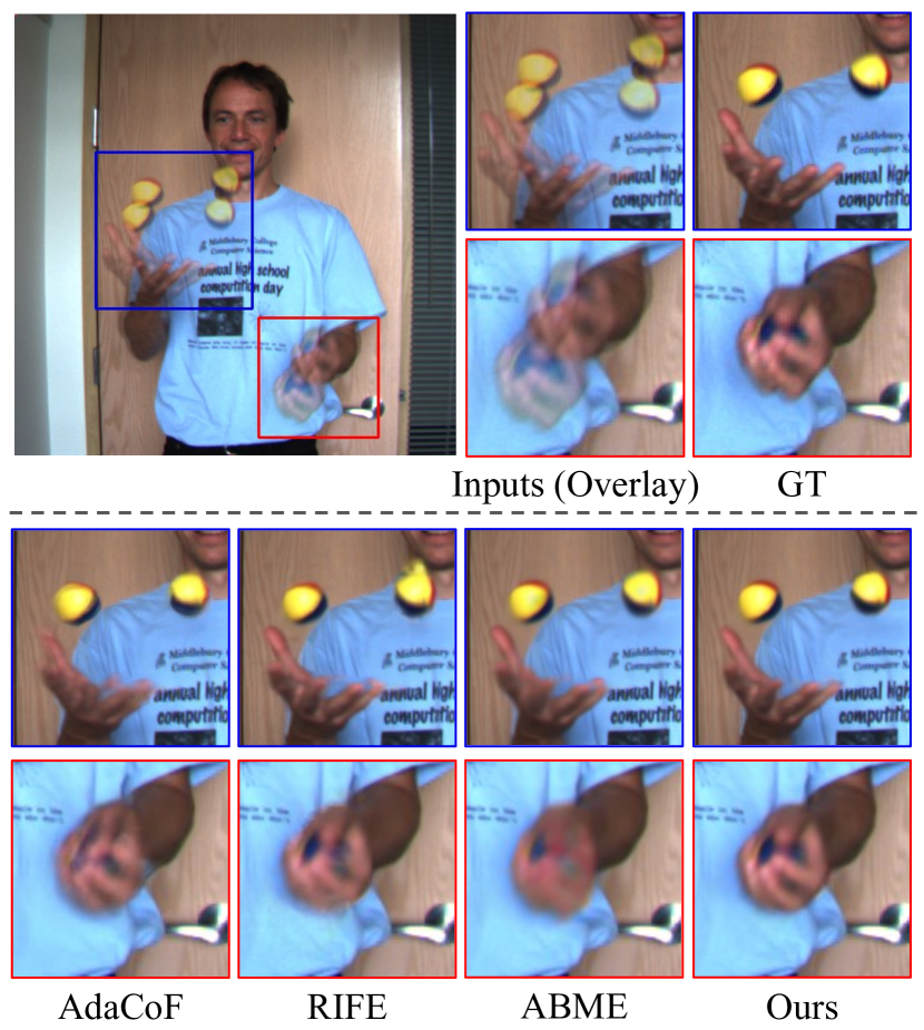
Figure 1: Visual comparison on a challenging sample from Middlebury dataset [1]. Our method produces the result more appealing than the three leading VFI methods, i.e., AdaCoF [22], RIFE [17] and ABME [37].

Since the vanilla Transformer needs high memory and computational cost, the proposed VFIformer is designed in a UNet [40] architecture where features are processed in different scales to reduce the computational complexity and enlarge the receptive field. Besides, to overcome the quadratic complexity, inspired by recent work [26, 47, 23, 11], our VFIformer is built upon window-based attention where feature maps are divided into non-overlapping sub-windows. Self-attention is only performed within each sub-window. Despite computationally efficient, such an approach prohibits information interaction between different windows and leads to limited receptive field. We address this problem by proposing cross-scale window-based attention, where the attention is computed among feature windows of different scales.

Our design enjoys two merits. (1) Compared with windows at the original scale, the corresponding windows at coarser scales cover more content. As a result, the interaction among these windows effectively enlarges the receptive field. (2) Features at coarser scales naturally contain smaller displacement and thus provide informative motion priors for the original scale to facilitate synthesis.

Our contributions are summarized as follows:

• We propose a novel framework integrated with the Transformer for the VFI task, which takes advantage of the Transformer to model long-range pixel correlations among the video frames.

• A cross-scale window-based attention mechanism is introduced to enlarge the receptive field of current window-based attention to adapt to the challenges of large motions in the VFI task.

• Our model achieves state-of-the-art performance for the VFI task on multiple public benchmarks.

2 Related Work

2.1 Video Frame Interpolation

Video frame interpolation, aiming to synthesize intermediate frames between existing ones of a video, is a long-standing problem. Existing methods can be classified into three categories. They are phase-based, kernel-based, and motion-based ones.

Phase-based methods represent motion in the phase shift of individual pixels. They interpolate phase and amplitude across the levels of a multi-scale pyramid through optimization [31] or neural networks [30]. A common drawback of these approaches is that they are only applicable to limited-range motion.

Kernel-based methods jointly perform motion estimation and motion compensation in a single step. Niklaus et al. [34] estimate a spatially-adaptive convolution kernel for each pixel using a convolutional network. The intermediate frame is then generated by convolving the input frames with the predicted kernels. Further development in this field includes using adaptive separable convolutions [35] to reduce network parameters, adopting deformable convolution or its alternatives to estimate both kernel weights and offset vectors [22, 41, 8], integrating optical flow and interpolation kernels together [3, 2] to improve the performance, and developing loss functions that combine adaptive convolution and trilinear interpolation [38].

These methods tend to yield blurry results when handling fast-moving objects since they hallucinate pixel values directly. Besides, to handle large motion, the estimated kernels are designed to be large, leading to a large number of parameters to learn.

For motion-based methods, optical flow is estimated to warp the input frames. Liu et al. [27] introduce a deep network that produces 3D optical flow vectors across space and time, and warps input frames by trilinear sampling. Jiang et al. [19] linearly combine optical flow between the input images to approximate the intermediate flow.

Recent work has explored a few strategies for improving the performance of such methods. These efforts include utilizing additional contextual information to interpolate high-quality results [32], developing unsupervised techniques by cycle consistency [39], detecting the occlusion by exploring the depth information [2], forward-warping input frames using softmax splatting [33], using quadratic interpolation to overcome the limitation of linear models [50, 24], leveraging the distillation loss to supervise the intermediate flows [17], and constructing efficient architectures for large resolution images [43, 10]. We note that methods built upon convolutional networks generally face challenges of modeling long-term dependencies thus limiting large motion handling.

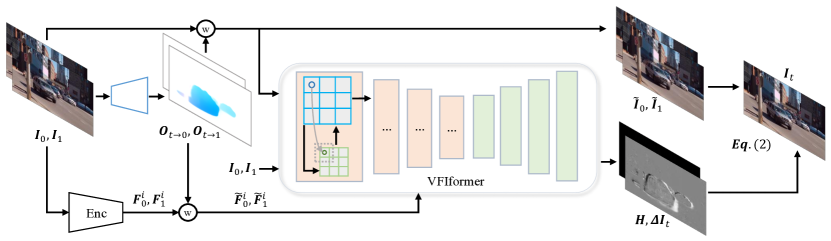
Figure 2: Overview of our proposed framework. At first, a convolutional network is used to directly estimate the intermediate optical flows $\bm{O}_{t\rightarrow 0}$ and $\bm{O}_{t\rightarrow 1}$. An encoder $Enc$ is used to extract multi-scale features $\bm{F}_{0}^{i}$ and $\bm{F}_{i}^{i}$ from the input frames, where $i=0,1,2,3$. The input frames and extracted features are then backward warped by the estimated flow, producing $\widetilde{\bm{I}}_{0}$, $\widetilde{\bm{I}}_{1}$, $\widetilde{\bm{F}}_{0}^{i}$, and $\widetilde{\bm{F}}_{1}^{i}$. At last, to generate the final results, the input frames and the warped features are fed into the proposed VFIformer, in which cross-scale attention is employed to enlarge the receptive field.

2.2 Transformer

Transformer was first proposed by Vaswani et al. [46] for machine translation. It consists of stacked self-attention layers for modeling dense relation among input tokens and has shown great flexibility. After breakthrough with the advent of Transformer in NLP, research of Transformer in computer vision becomes popular. Carion et al. [6] propose an end-to-end detection Transformer (DETR) for direct set prediction. Dosovitskiy et al. [14] propose ViT, which is a pure Transformer for image classification and achieves decent results. Liu et al. [26] present a general-purpose backbone, called Swin Transformer, which achieves linear computational complexity by computing self-attention within non-overlapping windows. A shifted window scheme is also proposed for cross-window connection.

Apart from high-level vision tasks, several attempts have also been made to integrate the Transformer into low-level vision tasks [52, 5, 7, 23]. Chen et al. [7] develop a pre-trained model for image processing using the Transformer architecture. Liang et al. [23] propose SwinIR for image restoration based on the Swin Transformer. Cao et al. [5] adapt Transformer for video super-resolution, and an optical flow-based feed-forward layer is integrated for feature alignment. In this work, we introduce the Transformer into the VFI task, aiming to leverage its power of capturing long-range correlation.

3 Our Method

Given two input frames $\bm{I}_{0}$ and $\bm{I}_{1}$, video frame interpolation is to synthesize an intermediate frame $\bm{I}_{t}$. Our framework is illustrated in Fig. 2. At first, we utilize a convolutional network (called flow estimator in the following) and an encoder $Enc$ to obtain the preliminary elements, including optical flows $\bm{O}_{t\rightarrow 0}$ and $\bm{O}_{t\rightarrow 1}$, corresponding warped features $\widetilde{\bm{F}}_{0}^{i}$ and $\widetilde{\bm{F}}_{1}^{i}$, and warped images $\widetilde{\bm{I}}_{0}$ and $\widetilde{\bm{I}}_{1}$.

With these preliminary results as input, VFIformer (Sec. 3.1) is utilized to capture long-range pixel interaction, generating the mask and residual for final synthesis. To enlarge the receptive field of the window-based attention in VFIformer, we design a cross-scale window-based attention (Sec. 3.2) mechanism to make trade-off between efficiency and performance.

3.1 VFIformer

Figure 3: Structure of the proposed VFIformer. (a) VFIformer is designed in a UNet architecture. Its encoder consists of several Transformer blocks (TFBs). (b) Structure of the Transformer blocks (TFB). (c) Structure of the Transformer layers (TFL), where Cross-Scale Window-based Attention (CSWA) is a key component.

Since the locality of convolution constrains its receptive field, previous VFI methods built upon convolutional networks generally face challenges of capturing long-range spatial interactions. In contrast, our work builds upon the recent advance that integrates Transformers into vision models to learn long-range dependencies. We propose the VFIformer, which is able to aggregate information over large receptive fields and is effective in handling large displacement.

As shown in Fig. 3a, our VFIformer is designed in a UNet architecture, where features are processed in different scales to reduce computational complexity and enlarge the receptive field. The encoder of VFIformer consists of several Transformer blocks (TFB), and the decoder consists of standard convolutions and transposed convolutions. For the $i$-th TFB, its output feature $F_{t}^{i}$ is produced as

$$\bm{F}_{t}^{i}={TFB}^{i}([\bm{F}_{t}^{i-1},\widetilde{\bm{F}}_{0}^{i},\widetilde{\bm{F}}_{1}^{i}])\;,$$ (1)

where $\bm{F}_{t}^{i-1}$ is the feature from the last TFB, $\widetilde{\bm{F}}_{0}^{i}$ and $\widetilde{\bm{F}}_{1}^{i}$ are the features from $Enc$ warped by the intermediate optical flow $\bm{O}_{t\rightarrow 0}$ and $\bm{O}_{t\rightarrow 1}$. ${TFB}^{i}$ denotes the operations of the $i$-th TFB. The first TFB takes as input the concatenation of frames $\bm{I}_{0}$, $\bm{I}_{1}$, $\widetilde{\bm{I}}_{0}$, and $\widetilde{\bm{I}}_{1}$ without features.

At last, the decoder of VFIformer produces a soft mask $\bm{H}$ and an image residual $\Delta\bm{I}_{t}$ to synthesize the final intermediate frame $\bm{I}_{t}$ as

$$\bm{I}_{t}=\bm{H}\odot\widetilde{\bm{I}}_{0}+(1-\bm{H})\odot\widetilde{\bm{I}}_{1}+\Delta{\bm{I}_{t}}\;,$$ (2)

where $\odot$ denotes the Hadamard product. The soft mask is used to blend the two warped frames $\widetilde{\bm{I}}_{0}$, $\widetilde{\bm{I}}_{1}$. The residual is used to compensate flow errors and occlusion.

We then look into the detailed structures of TFB. As illustrated in Fig. 3(b), each TFB consists of several Transformer layers TFL (see Fig. 3(c)) and convolutional layers. The features in the $l$-th TFL are processed as

$$\widehat{\bm{z}}^{l}=CSWA(LN(\bm{z}^{l-1}))+\bm{z}^{l-1}\;,$$ (3)

$$\bm{z}^{l}=MLP(LN(\widehat{\bm{z}}^{l}))+\widehat{\bm{z}}^{l},$$ (4)

where $\bm{z}^{l-1}$ is the feature generated by the $(l-1)$-th TFL. LN and MLP denote the LayerNorm and Multi-Layer Perceptrons. CSWA denotes our proposed cross-scale window-based attention, which is explained in the following.

3.2 Cross-Scale Window-based Attention (CSWA)

Window-based Attention (WA)

We first revisit the window-based attention method. Though the key component self-attention of Transformer, has shown great flexibility and strong modeling capability, a known fact is that its power comes at the price of high computational complexity. Inspired by [26, 23], we employ window-based attention (WA) to reduce the computational cost, where feature maps are divided into sub-windows. Self-attention is only performed within each sub-window. Specifically, for a feature map $\bm{F}\in\mathbb{R}^{H\times W\times C}$, we divide it into $\frac{HW}{M^{2}}$ sub-windows of size $M\times M$. Taking one of the windows $\bm{X}\in\mathbb{R}^{(M^{2},C)}$ as an example, its query, key and value matrices $\bm{Q}$, $\bm{K}$ and $\bm{V}\in\mathbb{R}^{(M^{2},d)}$ are computed as

$$\bm{Q}=\bm{X}\bm{W}_{Q},~{}~{}\bm{K}=\bm{X}\bm{W}_{K},~{}~{}\bm{V}=\bm{X}\bm{W}_{V}\;,$$ (5)

where $\bm{W}_{Q}$, $\bm{W}_{K}$, and $\bm{W}_{V}$ are projection matrices shared across different windows. Afterwards, the self-attention is computed as

$$Attn(\bm{Q},\bm{K},\bm{V})=Softmax(\frac{\bm{Q}\bm{K}^{T}}{\sqrt{d}}+\bm{P})\bm{V}\;,$$ (6)

where $\bm{P}$ is the learnable positional encoding, and $d$ is the $query/key$ dimension.

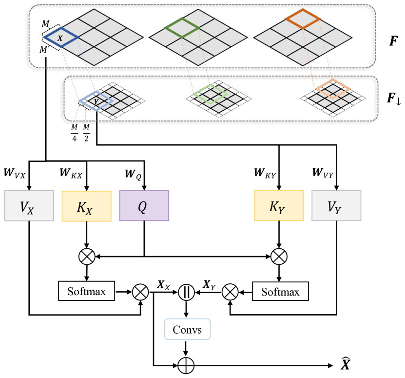
Figure 4: Proposed cross-scale window-based attention (CSWA). The fine-scale feature $\bm{F}$ is divided into non-overlapping windows (dark-colored block), and the coarse-scale feature $\bm{F}_{\downarrow}$ is divided into overlapping windows (light-colored block). The feature windows with the same color (e.g., $\bm{X}$ and $\bm{Y}$) interact with each other.

Cross-Scale Window-based Attention (CSWA)

Although window-based attention is computationally efficient, the drawback is that the receptive field is still limited, resulting in limited information interaction between different windows. We address this by introducing the cross-scale window-based attention (CSWA), which enlarges the receptive field in an effective way.

The details are shown in Fig. 4, for the input feature map $\bm{F}\in\mathbb{R}^{H\times W\times C}$, we first down-sample it by scale 2 to get $\bm{F}_{\downarrow}\in\mathbb{R}^{\frac{H}{2}\times\frac{W}{2}\times C}$. Then $\bm{F}$ is divided into $\frac{HW}{M^{2}}$ non-overlapping sub-windows, following the same procedure in WA as mentioned above. As for $\bm{F}_{\downarrow}$, we first pad it with padding size $\frac{M}{4}\times\frac{M}{4}$ in the mode of reflection, and then divide it into overlapping sub-windows of size $M\times M$.

Taking one of the windows $\bm{X}\in\mathbb{R}^{(M^{2},C)}$ in $\bm{F}$, we denote $\bm{Y}\in\mathbb{R}^{(M^{2},C)}$ as its corresponding window in $\bm{F}_{\downarrow}$. Following Eq. (5), we calculate the query $\bm{Q}$ only for the window $\bm{X}$ from the original feature $\bm{F}$. As for the key and value, we calculate them for both the window $\bm{X}$ and window $\bm{Y}$ to interact features in different scales. The procedure is written as

$$\bm{Q}=\bm{X}\bm{W}_{Q}\;,$$ (7)

$$\bm{K}_{X}=\bm{X}\bm{W}_{KX},~{}~{}\bm{K}_{Y}=\bm{Y}\bm{W}_{KY}\;,$$ (8)

$$\bm{V}_{X}=\bm{X}\bm{W}_{VX},~{}~{}\bm{V}_{Y}=\bm{Y}\bm{W}_{VY}\;,$$ (9)

where $\bm{W}_{Q}$, $\bm{W}_{KX}$, $\bm{W}_{KY}$, $\bm{W}_{VX}$ and $\bm{W}_{VY}$ are projection matrices. Afterwards, the attention is computed within the set of $(\bm{Q},\bm{K}_{X},\bm{V}_{X})$ and $(\bm{Q},\bm{K}_{Y},\bm{V}_{Y})$ in a similar way as Eq. (6), producing $\bm{X}_{X}$ and $\bm{X}_{Y}$. The final result is generated as

$$\hat{\bm{X}}=\bm{X}_{X}+Convs([\bm{X}_{X},\bm{X}_{Y}])\;,$$ (10)

where $[~{}]$ denotes concatenation in the channel dimension.

As shown in Fig. 4, windows with the same color of $\bm{F}$ and $\bm{F}_{\downarrow}$ interact with each other, introducing multi-scale information and therefore generating more representative features. On the other hand, windows of $\bm{F}_{\downarrow}$ cover larger context than those of $\bm{F}$. For example, window $\bm{Y}$ in $\bm{F}_{\downarrow}$ actually covers 4 times as much context as the window $\bm{X}$ in $\bm{F}$.

In this way, the receptive field of self-attention is enlarged effectively. We adopt the widely used effective receptive field (ERF) [28] to visualize the ERFs of WA and CSWA. Fig. 5 shows the ERF of a TFB equipped with left: WA, right: CSWA, it is obvious that the ERF of CSWA is much larger than that of WA.

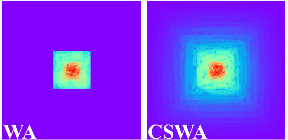
Figure 5: The effective receptive field of WA and CSWA.

3.3 Loss Functions

Reconstruction loss. We adopt $L_{1}$ loss as the reconstruction loss as

$$\mathcal{L}_{rec}=\|{\bm{I}}^{GT}_{t}-\bm{I}_{t}\|_{1}\;,$$ (11)

where $\bm{I}^{GT}_{t}$ and $\bm{I}_{t}$ denote the ground-truth intermediate frame and the generated one.

Census loss. Census loss [29, 54] $\mathcal{L}_{css}$ is robust to illumination changes, which is defined as the soft Hamming distance between census-transformed [53] image patches of $\bm{I}^{GT}_{t}$ and $\bm{I}_{t}$.

Distillation loss. Following [17], we use distillation loss to explicitly supervise the estimated flows as

$$\mathcal{L}_{dis}=\|\bm{O}^{*}_{t\rightarrow 0}-\bm{O}_{t\rightarrow 0}\|_{1}+\|\bm{O}^{*}_{t\rightarrow 1}-\bm{O}_{t\rightarrow 1}\|_{1}\;,$$ (12)

where $\bm{O}^{*}_{t\rightarrow 0}$ and $\bm{O}^{*}_{t\rightarrow 1}$ are flows generated by a pretrained flow estimation network [18]. $\bm{O}_{t\rightarrow 0}$ and $\bm{O}_{t\rightarrow 1}$ are flow estimated by our flow estimator.

Full objective. Our full objective is defined as

$$\mathcal{L}={\lambda}_{rec}\mathcal{L}_{rec}+{\lambda}_{css}\mathcal{L}_{css}+{\lambda}_{dis}\mathcal{L}_{dis}\;,$$ (13)

where ${\lambda}_{rec}$, ${\lambda}_{css}$ and ${\lambda}_{dis}$ are loss weights for $\mathcal{L}_{rec}$, $\mathcal{L}_{css}$ and $\mathcal{L}_{dis}$, respectively.

4 Experiments

4.1 Datasets

Our model is trained on the Vimeo90K training set and evaluated on various datasets.

Vimeo90K [51]. The Vimeo90K training set contains $51,312$ triplets, where each triplet consists of three consecutive video frames with resolution $448\times 256$. The Vimeo90K training set contains $3,782$ triplets whose resolution is also $448\times 256$.

UCF101 [44]. It contains videos with a large variety of human actions. There are 379 triplets with a resolution of $256\times 256$.

Middlebury. The Middlebury dataset has two subsets, in which the OTHER dataset provides the ground-truth intermediate frames. The image resolution in this dataset is around $640\times 480$. Following previous methods, we report the average interpolation error (IE) on the OTHER dataset. A lower IE indicates better performance.

SNU-FILM [9]. It contains $1,240$ triplets of resolutions up to $1280\times 720$. There are four different settings according to the motion types: Easy, Medium, Hard and Extreme.

Method	Vimeo90K	UCF101	Middlebury	SNU-FILM
				Easy	Medium	Hard	Extreme
ToFlow [51]	33.73/0.9682	34.58/0.9667	2.15	39.08/0.9890	34.39/0.9740	28.44/0.9180	23.39/0.8310
SepConv [35]	33.79/0.9702	34.78/0.9669	2.27	39.41/0.9900	34.97/0.9762	29.36/0.9253	24.31/0.8448
CyclicGen [25]	32.09/0.9490	35.11/0.9684	-	37.72/0.9840	32.47/0.9554	26.95/0.8871	22.70/0.8083
DAIN [2]	34.71/0.9756	34.99/0.9683	2.04	39.73/0.9902	35.46/0.9780	30.17/0.9335	25.09/0.8584
CAIN [9]	34.65/0.9730	34.91/0.9690	2.28	39.89/0.9900	35.61/0.9776	29.90/0.9292	24.78/0.8507
AdaCoF [22]	34.47/0.9730	34.90/0.9680	2.24	39.80/0.9900	35.05/0.9754	29.46/0.9244	24.31/0.8439
BMBC [36]	35.01/0.9764	35.15/0.9689	2.04	39.90/0.9902	35.31/0.9774	29.33/0.9270	23.92/0.8432
RIFE-Large [17]	36.10/0.9801	35.29/0.9693	1.94	40.02/0.9906	35.92/0.9791	30.49/0.9364	25.24/0.8621
ABME [37]	36.18/0.9805	35.38/0.9698	2.01	39.59/0.9901	35.77/0.9789	30.58/0.9364	25.42/0.8639
Ours	36.50/0.9816	35.43/0.9700	1.82	40.13/0.9907	36.09/0.9799	30.67/0.9378	25.43/0.8643

Table 1: Quantitative comparison among different VFI methods on 4 testing datasets. We report the average interpolation error IE (the lower the better) on the Middlebury dataset and report PSNR/SSIM (the higher the better) on other datasets. The best and second-best results are colored in red and blue.

	TFLs	CSWA	Vimeo90K	SNU-FILM
				Easy	Medium	Hard	Extreme
Model 1	✗	✗	36.27/0.9809	40.01/0.9906	35.89/0.9793	30.58/0.9369	25.33/0.8629
Model 2	✓	✗	36.49/0.9815	40.06/0.9907	36.03/0.9798	30.61/0.9375	25.40/0.8643
Model 3	✓	✓	36.50/0.9816	40.13/0.9907	36.09/0.9799	30.67/0.9378	25.43/0.8643

Table 2: Ablation study on the proposed modules.

4.2 Implementation Details

Network Achitecture. In the VFIformer, the window size is set to $8\times 8$, the channel numbers of linear layers and convolution layers are 180. Each TFB contains 6 TFLs except that the first TFB only contains 2 TFLs. Encoder $Enc$ contains 4 blocks and each extracts one level of features from $I_{0}$ and $I_{1}$. Each encoder block consists of 2 convolutions with strides 2 and 1, respectively, and the channel numbers of features are 24, 48, 96, and 192 from shallow to deep layers. The architecture of the flow estimator is included in the supplementary file.

Training Details. We train our model with the AdamW optimizer. The learning rate is set to $1e-4$. We first train the flow estimator for 0.32M iterations with batch size 48. Then the whole model is trained in an end-to-end manner for 0.47M iterations with batch size 24. The weight coefficients ${\lambda}_{rec}$, ${\lambda}_{css}$, and ${\lambda}_{dis}$ are 1, 1 and 0.01, respectively. We randomly crop $192\times 192$ patches from the training samples and augment them by random flip and time reversal.

4.3 Comparisons with State-of-the-Art Methods

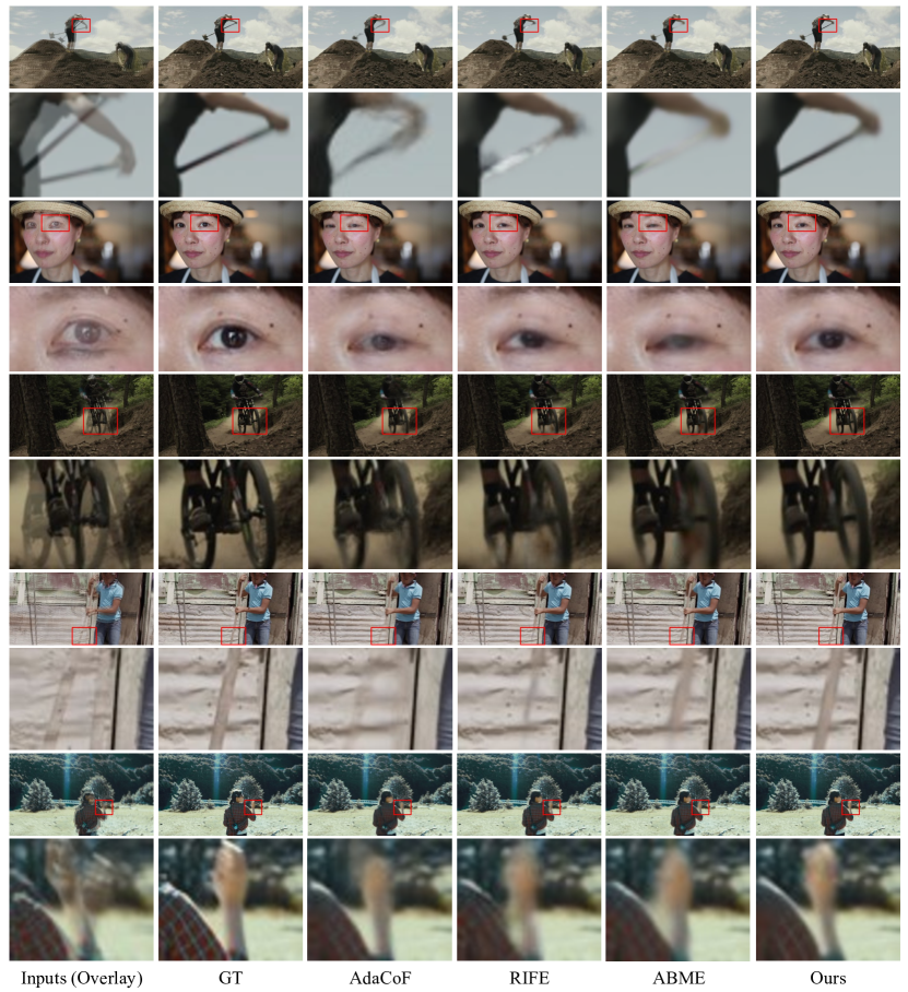
Figure 6: Visual comparison among different VFI methods on the Vimeo90K testing set.

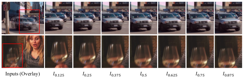
Figure 7: $8\times$ interpolation results of our method on the Vimeo90K testing set.

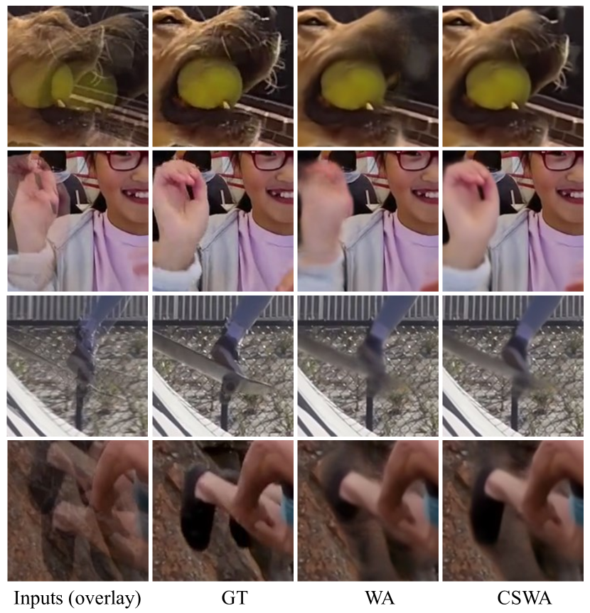
Figure 8: Ablation study on the cross-scale window-based attention (CSWA), the samples in the first and second columns are overlaid inputs and ground-truths. Those in the third and fourth are the results of the models without and with CSWA, respectively.

We compare our model with nine recent, competitive methods, including ToFlow [51], SepConv [35], CyclicGen [25], DAIN [2], CAIN [9], AdaCoF [22], BMBC [36], RIFE-Large [17] and ABME [37]. Table 1 shows the quantitative comparison, where the best and second best results are colored in red and blue. It is observed that our model outperforms recent state-of-the-art methods on all four testing sets. It is noteworthy that our method outperforms the second-best method on Vimeo90K testing set by 0.32 dB.

The visual comparison between our method and other VFI methods is shown in Fig. 6. Our proposed method generates more reasonable results with fewer unpleasing artifacts in general. For example, our method successfully interpolates the intermediate frame of the stick with large motion in the first and fourth example of Fig. 6.

Meanwhile, to thoroughly investigate the performance of our proposed method, we also conduct multi-frame generation. We recursively apply our model to generate multiple intermediate frames. Specifically, given two input frames $\bm{I}_{0}$ and $\bm{I}_{1}$, we first generate $\bm{I}_{0.5}$. Then we interpolate between $\bm{I}_{0}$ and $\bm{I}_{0.5}$ to generate $\bm{I}_{0.25}$. We show the $8\times$ interpolation results on Vimeo90K testing set in Fig. 7. Our model yields multiple intermediate frames with smooth motion.

Window Size	PSNR/SSIM
4	36.24/0.9806
8	36.29/0.9807
12	36.31/0.9808

Table 3: Ablation study on the window sizes of self-attention.

4.4 Ablation Study

In this section, we conduct several ablation studies to investigate our proposed method. We verify the effectiveness of the Transformer layers and the proposed cross-scale window-based attention. We also analyze the influence of different window sizes while computing attention.

Effect of the Transformer layers (TFLs). TFLs are the key components of our VFIformer, which play the role of capturing long-range dependency. We investigate the effect of TFLs by replacing them with convolutional layers of a similar number of parameters. The ablation results are shown in Table 2, where Model 2 is the model with TFLs (using standard window-based attention) and Model 1 is the model without TFLs. Model 2 outperforms Model 1 by 0.22 dB on the Vimeo90K testing set, and also obtains better performance on the SNU-FILM dataset under 4 settings.

Effect of Cross-scale Window-based Attention. Cross-scale window-based attention (CSWA) is proposed to enlarge the receptive field and aggregate multi-scale information. To further verify its effectiveness, we train two models with and without CSWA respectively. As shown in Table 2, Model 2 adopts standard window-based attention (WA) while Model 3 adopts CSWA.

Compared with Model 2, Model 3 improves it by 0.07, 0.06, and 0.06 dB in the Easy, Medium, and Hard settings of SNU-FILM, respectively, in terms of PSNR. We show the visual comparison of these two models on SNU-FILM (Hard) in Fig. 8. It is observed that compared with Model 2, Model 3 generates sharper results with more fine details while dealing with cases with large motion.

Influence of the Attention Window Size. We further investigate the influence of attention window size, which determines the size of the receptive field. The larger the window is, the larger the range of information can be captured, along with higher computational cost. To enable quick exploration, we train all the models for only 0.36M iterations in this experiment. Table 3 shows the ablation result. It is observed that the model with window size 12 achieves the best performance. To balance the performance and the computational cost, we choose window size 8 in our experiments.

5 Limitations

Though our proposed method has achieved decent results, there are several limitations. First, while our model is built upon the window-based attention, the computational cost is still heavier than CNN-based methods due to the complex calculations of self-attention. We will explore more efficient approaches in the future by computing self-attention in the horizontal and vertical stripes in parallel [13].

Second, unlike existing methods [19, 37] that are able to interpolate frames at arbitrary time, our model only synthesizes the intermediate frame. In future work, we will investigate variables that represent the interpolation time and put them into the network to control the generated content.

6 Conclusion

In this work, we have proposed a novel framework integrated with the Transformer for the video frame interpolation task. The proposed VFIformer endows our framework with a strong capability of modeling long-range dependencies and handling large motions. Further, a novel cross-scale window-based attention mechanism is designed to aggregate multi-scale information and enlarge the receptive field. Extensive experiments show that our proposed method achieves superior performance over existing state-of-the-art methods on multiple popular benchmarks.

Appendix A Appendix

A.1 More Implementation Details

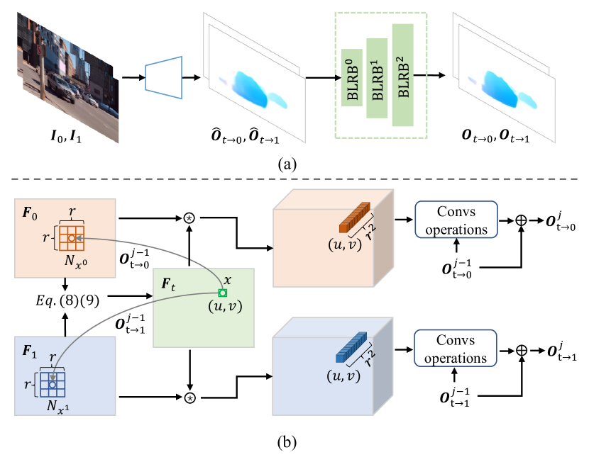
Figure 9: (a). The pipeline of our flow estimator, where the Bilateral Local Refinement Block (BLRB) is used to refine the flows. (b). Details of the Bilateral Local Refinement Block.

Flow Estimator Achitecture. The pipeline of our flow estimator is shown in Fig. 9a, a flow prediction network [17] is first used to predict the coarse flows $\hat{\bm{O}}_{t\rightarrow 0}$, $\hat{\bm{O}}_{t\rightarrow 1}$. Then Bilateral Local Refinement Blocks (BLRBs) are used to refine the flows in a coarse-to-fine manner, whose details are shown in Fig. 9b.

For the $j$-th BLRB, given the flows $\bm{O}^{j-1}_{t\rightarrow 0}$ and $\bm{O}^{j-1}_{t\rightarrow 1}$ produced by the last BLRB and feature maps $\bm{F}_{0}^{j}$, $\bm{F}_{1}^{j}$ of two input frames extracted by the encoder $Enc$, we first rescale the flows to the current scale (note that we do not change their notations after rescaling for brevity) and use them to backward warp the features, obtaining $\widetilde{\bm{F}}_{0}^{j}$ and $\widetilde{\bm{F}}_{1}^{j}$. Then the warped features are fed into convolutional layers to produce the intermediate feature $\bm{F}_{t}^{j}$. The specific process is given by

$$\bm{D}=sigmoid(Convs([\widetilde{\bm{F}}_{0}^{j},\widetilde{\bm{F}}_{1}^{j}]))\;,$$ (14)

$$\bm{F}_{t}^{j}=\bm{D}\odot\widetilde{\bm{F}}_{0}^{j}+(1-\bm{D})\odot\widetilde{\bm{F}}_{1}^{j}\;,$$ (15)

where $Convs$ denotes convolutional layers, $[~{}]$ denotes concatenation in the channel dimension, $\bm{D}$ is the generated mask for blending $\widetilde{\bm{F}}_{0}^{j}$ and $\widetilde{\bm{F}}_{1}^{j}$, and $sigmoid$ is used to ensure the mask in the range of [0, 1].

Afterwards, we compute the local correlation volumes to model the relationships among pixels in $\bm{F}_{t}^{j}$ and $\bm{F}_{0}^{j}$, $F_{1}^{j}$. Specifically, for each pixel $x=(u,v)$ in $\bm{F}_{t}^{j}$, we map it to its estimated correspondence in $\bm{F}_{0}^{j}$ (here we take refining $\hat{\bm{O}}^{j}_{t\rightarrow 0}$ for example): $x^{{}^{\prime}}=(u+\hat{\bm{O}}^{j-1}_{t\rightarrow 0}(u),v+\hat{\bm{O}}^{j-1}_{t\rightarrow 0}(v))$. Then a local window around $x^{{}^{\prime}}$ is defined as

$$\mathcal{N}_{x^{{}^{\prime}}}=\left\{(u+d_{u},v+dv)~{}|~{}d_{u},d_{v}\in\left\{-r,...,r\right\}\right\}\;,$$ (16)

where $r$ is the radius and is set to $1$ in our experiments. Then we calculate the cosine similarity between $x$ and pixels in $\mathcal{N}_{x^{{}^{\prime}}}$, producing a correlation vector. The correlation map is then processed by two convolutional layers. Meanwhile, the flow $\bm{O}^{j-1}_{t\rightarrow 0}$ is also processed with other two convolutional layers. At last, the correlation feature, the flow feature, $\bm{F}_{0}$ and $\bm{F}_{t}$ are concatenated and fed into four convolutional layers to produce the flow residual $\Delta\bm{O}^{j}_{t\rightarrow 0}$, the refined flow is obtained as

$$\bm{O}^{j}_{t\rightarrow 0}=\Delta\bm{O}^{j}_{t\rightarrow 0}+\bm{O}^{j-1}_{t\rightarrow 0}\;.$$ (17)

Note that all the operations are similar for $\bm{O}^{j}_{t\rightarrow 1}$.

A.2 More Ablation Studies

TFL number	PSNR/SSIM
2	36.35/0.9810
4	36.43/0.9814
6	36.49/0.9815
8	36.52/0.9817

Table 4: Ablation study on the TFL number.

Influence of the TFL number. We also investigate the influence of the TFL number, the ablation results on the Vimeo90K [51] testing set are shown in Table 4, we set the numbers of the TFLs in each TFB to 2, 4, 6, and 8, respectively. It is observed that the more TFLs, the higher PSNR/SSIM. To balance the performance and the computational cost, we set the number to 6 in our experiments.

Effect of CSWA. To have a thorough investigation on the Vimeo90K testing set, we split it into 4 motion levels according to the average flow values estimated by PWC-Net [45]. The PSNR gain of CSWA becomes larger as motions become larger as shown in Table 5, which further validates the effectiveness of CSWA.

flow range	avg. flow	WA	CSWA	gain
$[0,3)$	$1.9$	36.51	36.52	0.01
$[3,6)$	$4.0$	36.52	36.55	0.03
$[6,10)$	$7.4$	36.91	36.94	0.03
$[10,+\infty)$	$14.02$	34.00	34.04	0.04

Table 5: PSNR of WA and CSWA under 4 motion levels.

A.3 More Quantitative Comparisons

Methods	Runtime (ms)	Param. (M)	Vimeo90K
SoftSplat-$\mathcal{L}$ [33]	-	-	36.10/0.9700
CDFI [cdfi]	60	5.0	35.17/0.9640
XVFI [42]	96	5.5	35.07/0.9760
BMBC [36]	478	11.0	35.01/0.9764
RIFE-Large [17]	13	21.7	36.10/0.9801
ABME [37]	158	18.1	36.18/0.9805
Ours	365	24.1	36.50/0.9816
Ours-Small	213	17.0	36.38/0.9811

Table 6: More quantitative comparisons. The running time is tested on images with $448\times 256$ resolution on an NVIDIA TITAN V GPU.

We compare the running time and network parameters with some recent SOTA methods in Table 6. As mentioned in the Limitation section of the main paper, the computational cost of our model is still heavier than CNN-based methods. To increase the practicability of our model, we further train a light-weight version, which is denoted as ‘Ours-Small’. It adopts a simpler flow estimator architecture [17] and its window size and channel number are $4\times 4$ and 136. As shown in Table 6, the light-weight version has moderate running time and parameters yet still yields the SOTA result.

A.4 More Visual Results

More visual results are shown in Fig. 10 and Fig. 11. We compare our proposed method and other recent state-of-the-art methods, including AdaCoF [22], RIFE-Large [17] and ABME [37]. It can be observed that our method restores more appealing results with sharper structures.

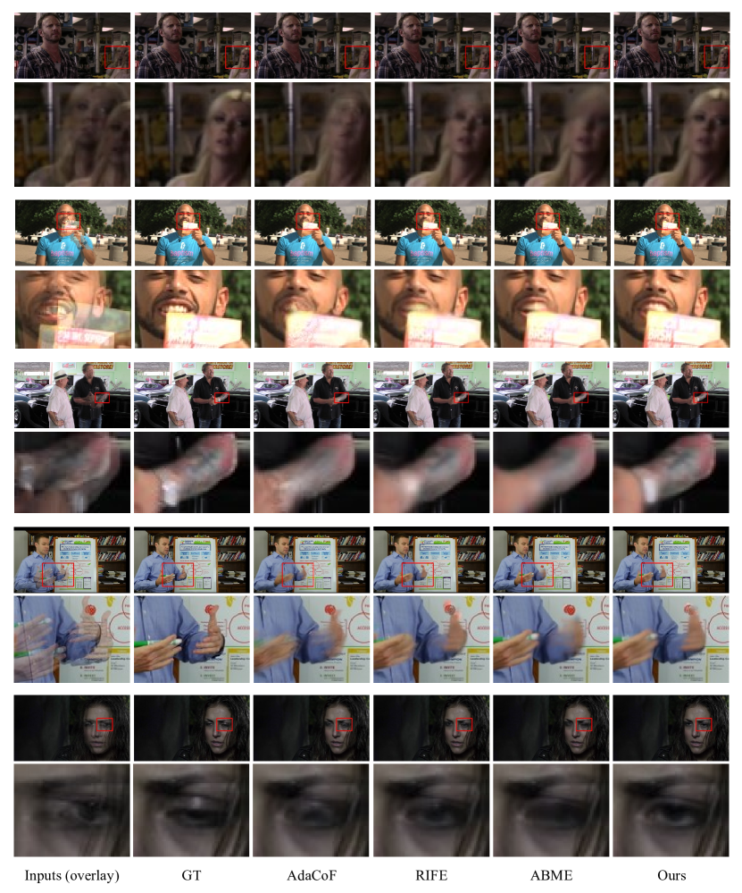
Figure 10: Visual comparison among different VFI methods on the Vimeo90K [51] testing set.

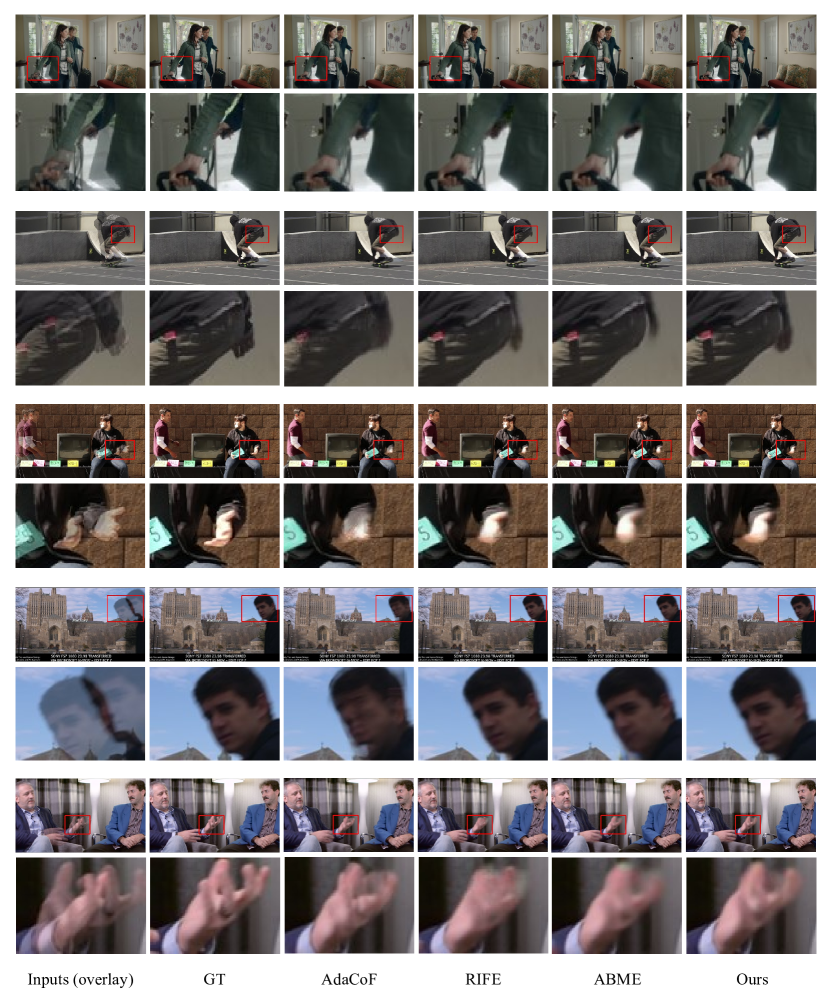
Figure 11: Visual comparison among different VFI methods on the Vimeo90K [51] testing set.

References

- [1] Simon Baker, Daniel Scharstein, JP Lewis, Stefan Roth, Michael J Black, and Richard Szeliski. A database and evaluation methodology for optical flow. International journal of computer vision, 92(1):1–31, 2011.
- [2] Wenbo Bao, Wei-Sheng Lai, Chao Ma, Xiaoyun Zhang, Zhiyong Gao, and Ming-Hsuan Yang. Depth-aware video frame interpolation. In Proceedings of the IEEE/CVF Conference on Computer Vision and Pattern Recognition, pages 3703–3712, 2019.
- [3] Wenbo Bao, Wei-Sheng Lai, Xiaoyun Zhang, Zhiyong Gao, and Ming-Hsuan Yang. Memc-net: Motion estimation and motion compensation driven neural network for video interpolation and enhancement. IEEE transactions on pattern analysis and machine intelligence, 2019.
- [4] Tom B Brown, Benjamin Mann, Nick Ryder, Melanie Subbiah, Jared Kaplan, Prafulla Dhariwal, Arvind Neelakantan, Pranav Shyam, Girish Sastry, Amanda Askell, et al. Language models are few-shot learners. arXiv preprint arXiv:2005.14165, 2020.
- [5] Jiezhang Cao, Yawei Li, Kai Zhang, and Luc Van Gool. Video super-resolution transformer. arXiv preprint arXiv:2106.06847, 2021.
- [6] Nicolas Carion, Francisco Massa, Gabriel Synnaeve, Nicolas Usunier, Alexander Kirillov, and Sergey Zagoruyko. End-to-end object detection with transformers. In European Conference on Computer Vision, pages 213–229. Springer, 2020.
- [7] Hanting Chen, Yunhe Wang, Tianyu Guo, Chang Xu, Yiping Deng, Zhenhua Liu, Siwei Ma, Chunjing Xu, Chao Xu, and Wen Gao. Pre-trained image processing transformer. In Proceedings of the IEEE/CVF Conference on Computer Vision and Pattern Recognition, pages 12299–12310, 2021.
- [8] Xianhang Cheng and Zhenzhong Chen. Multiple video frame interpolation via enhanced deformable separable convolution. IEEE Transactions on Pattern Analysis and Machine Intelligence, 2021.
- [9] Myungsub Choi, Heewon Kim, Bohyung Han, Ning Xu, and Kyoung Mu Lee. Channel attention is all you need for video frame interpolation. In Proceedings of the AAAI Conference on Artificial Intelligence, volume 34, pages 10663–10671, 2020.
- [10] Myungsub Choi, Suyoung Lee, Heewon Kim, and Kyoung Mu Lee. Motion-aware dynamic architecture for efficient frame interpolation. In Proceedings of the IEEE/CVF International Conference on Computer Vision, pages 13839–13848, 2021.
- [11] Xiangxiang Chu, Zhi Tian, Yuqing Wang, Bo Zhang, Haibing Ren, Xiaolin Wei, Huaxia Xia, and Chunhua Shen. Twins: Revisiting the design of spatial attention in vision transformers. arXiv preprint arXiv:2104.13840, 1(2):3, 2021.
- [12] Jacob Devlin, Ming-Wei Chang, Kenton Lee, and Kristina Toutanova. Bert: Pre-training of deep bidirectional transformers for language understanding. arXiv preprint arXiv:1810.04805, 2018.
- [13] Xiaoyi Dong, Jianmin Bao, Dongdong Chen, Weiming Zhang, Nenghai Yu, Lu Yuan, Dong Chen, and Baining Guo. Cswin transformer: A general vision transformer backbone with cross-shaped windows. arXiv preprint arXiv:2107.00652, 2021.
- [14] Alexey Dosovitskiy, Lucas Beyer, Alexander Kolesnikov, Dirk Weissenborn, Xiaohua Zhai, Thomas Unterthiner, Mostafa Dehghani, Matthias Minderer, Georg Heigold, Sylvain Gelly, et al. An image is worth 16x16 words: Transformers for image recognition at scale. arXiv preprint arXiv:2010.11929, 2020.
- [15] John Flynn, Ivan Neulander, James Philbin, and Noah Snavely. Deepstereo: Learning to predict new views from the world’s imagery. In Proceedings of the IEEE conference on computer vision and pattern recognition, pages 5515–5524, 2016.
- [16] Muhammad Haris, Greg Shakhnarovich, and Norimichi Ukita. Space-time-aware multi-resolution video enhancement. In Proceedings of the IEEE/CVF Conference on Computer Vision and Pattern Recognition, pages 2859–2868, 2020.
- [17] Zhewei Huang, Tianyuan Zhang, Wen Heng, Boxin Shi, and Shuchang Zhou. Rife: Real-time intermediate flow estimation for video frame interpolation. arXiv preprint arXiv:2011.06294, 2020.
- [18] Tak-Wai Hui, Xiaoou Tang, and Chen Change Loy. Liteflownet: A lightweight convolutional neural network for optical flow estimation. In Proceedings of the IEEE conference on computer vision and pattern recognition, pages 8981–8989, 2018.
- [19] Huaizu Jiang, Deqing Sun, Varun Jampani, Ming-Hsuan Yang, Erik Learned-Miller, and Jan Kautz. Super slomo: High quality estimation of multiple intermediate frames for video interpolation. In Proceedings of the IEEE Conference on Computer Vision and Pattern Recognition, pages 9000–9008, 2018.
- [20] Nima Khademi Kalantari, Ting-Chun Wang, and Ravi Ramamoorthi. Learning-based view synthesis for light field cameras. ACM Transactions on Graphics (TOG), 35(6):1–10, 2016.
- [21] Soo Ye Kim, Jihyong Oh, and Munchurl Kim. Fisr: deep joint frame interpolation and super-resolution with a multi-scale temporal loss. In Proceedings of the AAAI Conference on Artificial Intelligence, volume 34, pages 11278–11286, 2020.
- [22] Hyeongmin Lee, Taeoh Kim, Tae-young Chung, Daehyun Pak, Yuseok Ban, and Sangyoun Lee. Adacof: Adaptive collaboration of flows for video frame interpolation. In Proceedings of the IEEE/CVF Conference on Computer Vision and Pattern Recognition, pages 5316–5325, 2020.
- [23] Jingyun Liang, Jiezhang Cao, Guolei Sun, Kai Zhang, Luc Van Gool, and Radu Timofte. Swinir: Image restoration using swin transformer. In Proceedings of the IEEE/CVF International Conference on Computer Vision, pages 1833–1844, 2021.
- [24] Yihao Liu, Liangbin Xie, Li Siyao, Wenxiu Sun, Yu Qiao, and Chao Dong. Enhanced quadratic video interpolation. In European Conference on Computer Vision, pages 41–56. Springer, 2020.
- [25] Yu-Lun Liu, Yi-Tung Liao, Yen-Yu Lin, and Yung-Yu Chuang. Deep video frame interpolation using cyclic frame generation. In Proceedings of the AAAI Conference on Artificial Intelligence, volume 33, pages 8794–8802, 2019.
- [26] Ze Liu, Yutong Lin, Yue Cao, Han Hu, Yixuan Wei, Zheng Zhang, Stephen Lin, and Baining Guo. Swin transformer: Hierarchical vision transformer using shifted windows. arXiv preprint arXiv:2103.14030, 2021.
- [27] Ziwei Liu, Raymond A Yeh, Xiaoou Tang, Yiming Liu, and Aseem Agarwala. Video frame synthesis using deep voxel flow. In Proceedings of the IEEE International Conference on Computer Vision, pages 4463–4471, 2017.
- [28] Wenjie Luo, Yujia Li, Raquel Urtasun, and Richard Zemel. Understanding the effective receptive field in deep convolutional neural networks. In NeurIPS, pages 4905–4913, 2016.
- [29] Simon Meister, Junhwa Hur, and Stefan Roth. Unflow: Unsupervised learning of optical flow with a bidirectional census loss. In Thirty-Second AAAI Conference on Artificial Intelligence, 2018.
- [30] Simone Meyer, Abdelaziz Djelouah, Brian McWilliams, Alexander Sorkine-Hornung, Markus Gross, and Christopher Schroers. Phasenet for video frame interpolation. In Proceedings of the IEEE Conference on Computer Vision and Pattern Recognition, pages 498–507, 2018.
- [31] Simone Meyer, Oliver Wang, Henning Zimmer, Max Grosse, and Alexander Sorkine-Hornung. Phase-based frame interpolation for video. In Proceedings of the IEEE conference on computer vision and pattern recognition, pages 1410–1418, 2015.
- [32] Simon Niklaus and Feng Liu. Context-aware synthesis for video frame interpolation. In Proceedings of the IEEE conference on computer vision and pattern recognition, pages 1701–1710, 2018.
- [33] Simon Niklaus and Feng Liu. Softmax splatting for video frame interpolation. In Proceedings of the IEEE/CVF Conference on Computer Vision and Pattern Recognition, pages 5437–5446, 2020.
- [34] Simon Niklaus, Long Mai, and Feng Liu. Video frame interpolation via adaptive convolution. In Proceedings of the IEEE Conference on Computer Vision and Pattern Recognition, pages 670–679, 2017.
- [35] Simon Niklaus, Long Mai, and Feng Liu. Video frame interpolation via adaptive separable convolution. In Proceedings of the IEEE International Conference on Computer Vision, pages 261–270, 2017.
- [36] Junheum Park, Keunsoo Ko, Chul Lee, and Chang-Su Kim. Bmbc: Bilateral motion estimation with bilateral cost volume for video interpolation. In Computer Vision–ECCV 2020: 16th European Conference, Glasgow, UK, August 23–28, 2020, Proceedings, Part XIV 16, pages 109–125. Springer, 2020.
- [37] Junheum Park, Chul Lee, and Chang-Su Kim. Asymmetric bilateral motion estimation for video frame interpolation. In Proceedings of the IEEE/CVF International Conference on Computer Vision, pages 14539–14548, 2021.
- [38] Tomer Peleg, Pablo Szekely, Doron Sabo, and Omry Sendik. Im-net for high resolution video frame interpolation. In Proceedings of the IEEE/CVF Conference on Computer Vision and Pattern Recognition, pages 2398–2407, 2019.
- [39] Fitsum A Reda, Deqing Sun, Aysegul Dundar, Mohammad Shoeybi, Guilin Liu, Kevin J Shih, Andrew Tao, Jan Kautz, and Bryan Catanzaro. Unsupervised video interpolation using cycle consistency. In Proceedings of the IEEE/CVF International Conference on Computer Vision, pages 892–900, 2019.
- [40] Olaf Ronneberger, Philipp Fischer, and Thomas Brox. U-net: Convolutional networks for biomedical image segmentation. In International Conference on Medical image computing and computer-assisted intervention, pages 234–241. Springer, 2015.
- [41] Zhihao Shi, Xiaohong Liu, Kangdi Shi, Linhui Dai, and Jun Chen. Video interpolation via generalized deformable convolution. arXiv e-prints, pages arXiv–2008, 2020.
- [42] Hyeonjun Sim, Jihyong Oh, and Munchurl Kim. Xvfi: Extreme video frame interpolation. In Proceedings of the IEEE/CVF International Conference on Computer Vision, pages 14489–14498, 2021.
- [43] Hyeonjun Sim, Jihyong Oh, and Munchurl Kim. Xvfi: Extreme video frame interpolation. In Proceedings of the IEEE/CVF International Conference on Computer Vision, pages 14489–14498, 2021.
- [44] Khurram Soomro, Amir Roshan Zamir, and Mubarak Shah. Ucf101: A dataset of 101 human actions classes from videos in the wild. arXiv preprint arXiv:1212.0402, 2012.
- [45] Deqing Sun, Xiaodong Yang, Ming-Yu Liu, and Jan Kautz. Pwc-net: Cnns for optical flow using pyramid, warping, and cost volume. In Proceedings of the IEEE conference on computer vision and pattern recognition, pages 8934–8943, 2018.
- [46] Ashish Vaswani, Noam Shazeer, Niki Parmar, Jakob Uszkoreit, Llion Jones, Aidan N Gomez, Łukasz Kaiser, and Illia Polosukhin. Attention is all you need. In Advances in neural information processing systems, pages 5998–6008, 2017.
- [47] Zhendong Wang, Xiaodong Cun, Jianmin Bao, and Jianzhuang Liu. Uformer: A general u-shaped transformer for image restoration. arXiv preprint arXiv:2106.03106, 2021.
- [48] Chao-Yuan Wu, Nayan Singhal, and Philipp Krahenbuhl. Video compression through image interpolation. In Proceedings of the European Conference on Computer Vision (ECCV), pages 416–431, 2018.
- [49] Xiaoyu Xiang, Yapeng Tian, Yulun Zhang, Yun Fu, Jan P Allebach, and Chenliang Xu. Zooming slow-mo: Fast and accurate one-stage space-time video super-resolution. In Proceedings of the IEEE/CVF conference on computer vision and pattern recognition, pages 3370–3379, 2020.
- [50] Xiangyu Xu, Li Siyao, Wenxiu Sun, Qian Yin, and Ming-Hsuan Yang. Quadratic video interpolation. arXiv preprint arXiv:1911.00627, 2019.
- [51] Tianfan Xue, Baian Chen, Jiajun Wu, Donglai Wei, and William T Freeman. Video enhancement with task-oriented flow. International Journal of Computer Vision, 127(8):1106–1125, 2019.
- [52] Fuzhi Yang, Huan Yang, Jianlong Fu, Hongtao Lu, and Baining Guo. Learning texture transformer network for image super-resolution. In Proceedings of the IEEE/CVF Conference on Computer Vision and Pattern Recognition, pages 5791–5800, 2020.
- [53] Ramin Zabih and John Woodfill. Non-parametric local transforms for computing visual correspondence. In European conference on computer vision, pages 151–158. Springer, 1994.
- [54] Yiran Zhong, Pan Ji, Jianyuan Wang, Yuchao Dai, and Hongdong Li. Unsupervised deep epipolar flow for stationary or dynamic scenes. In Proceedings of the IEEE/CVF Conference on Computer Vision and Pattern Recognition, pages 12095–12104, 2019.