Optimal error estimates of multiphysics finite element method for a nonlinear poroelasticity model with nonlinear stress-strain relations

Abstract

In this paper, we study the numerical algorithm for a nonlinear poroelasticity model with nonlinear stress-strain relations. By using variable substitution, the original problem can be reformulated to a new coupled fluid-fluid system, that is, a generalized nonlinear Stokes problem of displacement vector field related to pseudo pressure and a diffusion problem of other pseudo pressure fields. A new technique is used to get the existence and uniqueness of the solution of the reformulated model and a fully discrete nonlinear finite element method is proposed to solve the model numerically. The multiphysics finite element is used to get the discretization of the space variable and the backward Euler method is taken as the time-stepping method in the fully discrete case. Stability analysis and the error estimation are given for the fully discrete case and numerical test are taken to verify the theoretical results.

1 Introduction

Poromechanic is a fluid-solid interaction system at pore scale and is a branch of continuum mechanics and acoustics. If the solid is an elastic material, then the subject of the study is known as poroelasticity. Moreover, the elastic material may be governed by linear or nonlinear constitutive law, which then leads respectively to linear and nonlinear poroelasticity. The quasi-static poroelasticity model to be studied in this paper is given as (cf. [1, 2, 3]):

(1.1) $$-{\mbox{\rm div\,}}\sigma(\mathbf{u})+\alpha\nabla p =\mathbf{f} \qquad\mbox{in }\Omega_{T}:=\Omega\times(0,T)\subset\mathbf{\mathbb{R}}^{d}\times(0,T),$$

(1.2) $$(c_{0}p+\alpha{\mbox{\rm div\,}}\mathbf{u})_{t}+{\mbox{\rm div\,}}\mathbf{v}_{f} =\phi \qquad\mbox{in }\Omega_{T},$$

where

(1.3) $$\mathbf{v}_{f} :=-\frac{K}{\mu_{f}}\bigl{(}\nabla p-\rho_{f}\mathbf{g}\bigr{)}.$$

Here $\Omega\subset\mathbb{R}^{d}\,(d=1,2,3)$ denotes a bounded polygonal domain with the boundary ${\partial}\Omega$. And $\mathbf{u}$ denotes the displacement vector of the solid and $p$ denotes the pressure of the solvent. $\mathbf{f}$ is the body force, $\mathbf{g}$ is the gravitational acceleration. $I$ denotes the $d\times d$ identity matrix. The permeability tensor $K=K(x)$ is assumed to be symmetric and uniformly positive definite in the sense that there exists positive constants $K_{1}$ and $K_{2}$ such that $K_{1}|\zeta|^{2}\leq K(x)\zeta\cdot\zeta\leq K_{2}|\zeta|^{2}$ for a.e. $x\in\Omega$ and any $\zeta\in\mathbf{\mathbb{R}}^{d}$. The solvent viscosity $\mu_{f}$, Biot-Willis constant $\alpha$, and the constrained specific storage coefficient $c_{0}$ are all positive. In addition, $\sigma(\mathbf{u})$ is called the nonlinear (effective) stress tensor, $\widehat{\sigma}(\mathbf{u},p):=\sigma(\mathbf{u})-\alpha pI$ is the total stress tensor. $\mathbf{v}_{f}$ is the volumetric solvent flux and (1.3) is the well-known Darcy’s law, and $\rho_{f}$ is a positive constant.

To close the system (1.1)-(1.2), the following set of boundary and initial conditions will be considered in this paper:

(1.4) $$\widehat{\sigma}(\mathbf{u},p)\mathbf{n}=\sigma(\mathbf{u})\mathbf{n}-\alpha p\mathbf{n} =\mathbf{f}_{1} \qquad\mbox{on }{\partial}\Omega_{T}:={\partial}\Omega\times(0,T),$$

(1.5) $$\mathbf{v}_{f}\cdot\mathbf{n}=-\frac{K}{\mu_{f}}\bigl{(}\nabla p-\rho_{f}\mathbf{g}\bigr{)}\cdot\mathbf{n} =\phi_{1} \qquad\mbox{on }{\partial}\Omega_{T},$$

(1.6) $$\mathbf{u}=\mathbf{u}_{0},\qquad p =p_{0} \qquad\mbox{in }\Omega\times\{t=0\}.$$

We remark that poroelasticity model (1.1)-(1.2) has been widely applied in many fields such as material science, biomechanics and so on, for the details, one can see [4, 5, 2] and the references therein. Especially, the nonlinear poroelasticity model has been used to simulate the activity process of some biological tissues, for example, nonlinear poroelasticity model can be used to study soft tissue of orbit and mechanical mechanism of lung and other organs in human body, one can refer to [6, 7] and the references therein. Due to the complexity of nonlinear poroelasticity, there are few of theoretical results, as for the numerical results for the nonlinear poroelasticity problem, Levenston and Frank proposed a three-field (displacement, fluid flux, pressure) formula in [8], Chapelle and Gerbeau et al. proposed the operator splitting iteration method in [9], Berger, Bordas and Kay developed a stabilized low-order three-field mixed finite element method in [10] for the fully saturated incompressible small deformation case for which a linearly elastic model is sufficient. The low-order finite element method is relatively easy to implement and allows effective preconditioning by [11, 12, 13]. Vuong, Yoshihara and Wall use a three-field finite element method which is continuous in pressure in [14]. Berger, Bordas, Kay and Tavener construct a stabilized finite-element method to compute flow and finite-strain deformations in an incompressible poroelastic medium in [15], where the authors employ a three-field mixed formulation to calculate displacement, fluid flux and pressure directly and introduce a Lagrange multiplier to enforce flux boundary conditions. The authors of [1, 16] use the finite element method to solve the poroelasticity model directly and it will appear locking phenomenon. Recently, a HHO method is proposed for nonlinear poroelasticity and elasticity in [17] and [18]. As for the permeability tensor $K({\mbox{\rm div\,}}\mathbf{u})$ of nonlinear poroelasticity, one can refer to [19, 20, 21, 22, 24, 23, 25] and the references therein. At the same time, another main difficulty is how to decouple the coupled system and how to deal with the nonlinear terms in computation. In this work, we follow the method used in [3] to get the numerical algorithm. By introducing a new variable $q={\rm{\mbox{\rm div\,}}}\mathbf{u}$ and a new denotation $\mathcal{N}(\varepsilon(\mathbf{u}))=\sigma(\mathbf{u})-\lambda\mathrm{div}\mathbf{u}\textit{I}$, where Lamé constant $\lambda$ is computed from the Young’s modulus $E$ and the Poisson ratio $\nu$ by $\lambda=\frac{E\nu}{(1+\nu)(1-2\nu)}$, we reformulate the nonlinear poroelasticity problem into a generalized nonlinear Stokes problem for the displacement vector field and pseudo pressure field and a diffusion problem for other pseudo pressure fields. To the best of our knowledge, there are few existing references to use the fully discrete multiphysics finite element method to study the nonlinear poroelasticity. In this work, the multiphysics nonlinear finite element method is used to solve the space variables, and the Newton iteration method is used to solve the nonlinear equations, and the backward Euler method is used to get the time discretization. The main novelty is that the multiphysics nonlinear finite element method is used and the error estimate is made for the numerical method.

This paper is organized as follows. In Section 2, we introduce the reformulated multiphysics model for the nonlinear poroelasticity and give the PDE analysis. In Section 3, we propose a fully discrete multiphysics nonlinear finite element method for the poroelasticity model, and give the stability analysis and convergence analysis of the multiphysics nonlinear finite element method. In Section 4, we present the numerical results to verify the efficiency of the proposed numerical methods. Finally, we draw a conclusion to summary the main works in this paper.

2 Multiphysics reformulation and its PDE analysis

2.1 Multiphysics reformulation

To reveal the multi-physics progresses and to propose absolutely stable and high order numerical method, we firstly derive a multiphysics reformulation for the original model, and then make numerical approximation for the reformulated model. This is a key idea of this work and it will be seen in the later sections that this new approach is advantageous. To the end, we introduce new variable $q:={\mbox{\rm div\,}}\mathbf{u}$, and denote

$$\mathcal{N}(\varepsilon(\mathbf{u})):~{}=\sigma(\mathbf{u})-\lambda q\textit{I},\quad\eta:=c_{0}p+\alpha q,\quad\xi:=\alpha p-\lambda q,$$

where $\varepsilon(\mathbf{u})=\frac{1}{2}(\nabla\mathbf{u}+\nabla\mathbf{u}^{T})$.

It is easy to check that

(2.1) $$p=\kappa_{1}\xi+\kappa_{2}\eta,\qquad q=\kappa_{1}\eta-\kappa_{3}\xi,$$

where

(2.2) $$\kappa_{1}:=\frac{\alpha}{\alpha^{2}+\lambda c_{0}},\quad\kappa_{2}:=\frac{\lambda}{\alpha^{2}+\lambda c_{0}},\quad\kappa_{3}:=\frac{c_{0}}{\alpha^{2}+\lambda c_{0}}.$$

Then (1.1)-(1.2) can be written as

(2.3) $$-{\mbox{\rm div\,}}\mathcal{N}(\varepsilon(\mathbf{u}))+\nabla\xi =\mathbf{f} \qquad\mbox{in }\Omega_{T},$$

(2.4) $$\kappa_{3}\xi+{\mbox{\rm div\,}}\mathbf{u} =\kappa_{1}\eta \qquad\mbox{in }\Omega_{T},$$

(2.5) $$\eta_{t}-\frac{1}{\mu_{f}}{\mbox{\rm div\,}}[K(\nabla(\kappa_{1}\xi+\kappa_{2}\eta)-\rho_{f}\mathbf{g})] =\phi \qquad\mbox{in }\Omega_{T},$$

where $p$ and $q$ are related to $\xi$ and $\eta$ through the algebraic equations in (2.1).

The boundary and initial conditions (1.4)-(1.6) can be rewritten as

(2.6) $$\sigma(\mathbf{u})\mathbf{n}-\alpha(\kappa_{1}\xi+\kappa_{2}\eta)\mathbf{n} =\mathbf{f}_{1} \qquad\mbox{on }{\partial}\Omega_{T},$$

(2.7) $$-\frac{K}{\mu_{f}}\bigl{(}\nabla(\kappa_{1}\xi+\kappa_{2}\eta)-\rho_{f}\mathbf{g}\bigr{)}\cdot\mathbf{n} =\phi_{1} \qquad\mbox{on }{\partial}\Omega_{T},$$

(2.8) $$\mathbf{u}=\mathbf{u}_{0},\qquad p =p_{0} \qquad\mbox{in }\Omega\times\{t=0\}.$$

Remark 2.1.

It is clear that $(\mathbf{u},\xi)$ satisfies a generalized nonlinear Stokes problem for a given $\eta$, where $\kappa_{3}\xi$ in (2.4) acts as a penalty term, and $\eta$ satisfies a diffusion problem for a given $\xi$. This new formulation reveals the underlying deformation and diffusion processes which occurs in the poroelastic material.

Remark 2.2.

The original pressure is eliminated in the reformulation, which will be helpful to overcome the “locking phenomenon”, the later numerical tests show that our proposed method has no “locking phenomenon” ( see Section 4).

To define the weak solution, we need the standard function space notation, one can see [26, 27, 28] for details. In particular, $(\cdot,\cdot)$ and $\langle\cdot,\cdot\rangle$ denote respectively the standard $L^{2}(\Omega)$ and $L^{2}({\partial}\Omega)$ inner products. For any Banach space $B$, we let $\mathbf{B}=[B]^{d}$, and use $\mathbf{B}^{\prime}$ to denote its dual space. In particular, we use $(\cdot,\cdot)$ to denote the dual product on $\mathbf{H}^{1}(\Omega)^{\prime}\times\mathbf{H}^{1}(\Omega)$, and $\|\,\cdot\,\|_{L^{p}(B)}$ is a shorthand notation for $\|\,\cdot\,\|_{L^{p}((0,T);B)}$.

Letting $A=(a_{ij})_{n\times n}$, we respectively define the product $(A,A)$, $F$-norm $\|A\|_{F}$ and the $L^{2}$-norm $\|A\|_{L^{2}(\Omega)}$ of the matrix by

(2.9) $$\|A\|_{F}=:(A:A)^{\frac{1}{2}}=:(\sum_{i,j=1}^{n}a_{ij}^{2})^{\frac{1}{2}},$$

(2.10) $$(A,A)=\int_{\Omega}A:Adx=:\|A\|_{L^{2}(\Omega)}({\rm or\ denoted\ by}\ \|A\|_{L^{2}}).$$

We also introduce the function spaces

$$L^{2}_{0}(\Omega):=\{q\in L^{2}(\Omega);\,(q,1)=0\},\qquad\mathbf{X}:=\mathbf{H}^{1}(\Omega).$$

From [28], it is well known that the following so-called inf-sup condition holds in the space $\mathbf{X}\times L^{2}_{0}(\Omega)$:

(2.11) $$\sup_{\mathbf{v}\in\mathbf{X}}\frac{({\mbox{\rm div\,}}\mathbf{v},\varphi)}{\|\,\mathbf{v}\,\|_{H^{1}(\Omega)}}\geq\alpha_{0}\|\,\varphi\,\|_{L^{2}(\Omega)}\qquad\forall\varphi\in L^{2}_{0}(\Omega),\quad\alpha_{0}>0.$$

Let

$$\mathbf{RM}:=\{\mathbf{r}:=\mathbf{a}+\mathbf{b}\times x;\,\mathbf{a},\mathbf{b},x\in\mathbb{R}^{d}\}$$

denotes the space of infinitesimal rigid motions. From [29, 30, 28], it is well known that $\mathbf{RM}$ is the kernel of the strain operator $\varepsilon$, that is, $\mathbf{r}\in\mathbf{RM}$ if and only if $\varepsilon(\mathbf{r})=0$. Hence, we have

(2.12) $$\varepsilon(\mathbf{r})=0,\quad{\mbox{\rm div\,}}\mathbf{r}=0\qquad\forall\mathbf{r}\in\mathbf{RM}.$$

$\mathbf{L}^{2}_{\bot}({\partial}\Omega)$ and $\mathbf{H}^{1}_{\bot}(\Omega)$ denote respectively the subspaces of $\mathbf{L}^{2}({\partial}\Omega)$ and $\mathbf{H}^{1}(\Omega)$ which are orthogonal to $\mathbf{RM}$, that is,

$$\mathbf{H}^{1}_{\bot}(\Omega):=\{\mathbf{v}\in\mathbf{H}^{1}(\Omega);\,(\mathbf{v},\mathbf{r})=0\,\,\forall\mathbf{r}\in\mathbf{RM}\},$$

$$\mathbf{L}^{2}_{\bot}({\partial}\Omega):=\{\mathbf{g}\in\mathbf{L}^{2}({\partial}\Omega);\,\langle\mathbf{g},\mathbf{r}\rangle=0\,\,\forall\mathbf{r}\in\mathbf{RM}\}.$$

Next, we define the weak solutions to problem (1.1)–(1.6). For convenience, we assume that $\mathbf{f},\mathbf{f}_{1},\phi$ and $\phi_{1}$ all are independent of $t$ in the remaining of the paper. Note that all the results of this paper can be easily extended to the case of time-dependent source functions.

Definition 1.

Let $\mathbf{u}_{0}\in\mathbf{H}^{1}(\Omega),\mathbf{f}\in\mathbf{L}^{2}(\Omega),\mathbf{f}_{1}\in\mathbf{L}^{2}({\partial}\Omega),p_{0}\in L^{2}(\Omega),\phi\in L^{2}(\Omega)$, and $\phi_{1}\in L^{2}({\partial}\Omega)$. Assume $c_{0}>0$ and $(\mathbf{f},\mathbf{v})+\langle\mathbf{f}_{1},\mathbf{v}\rangle=0$ for any $\mathbf{v}\in\mathbf{RM}$. Given $T>0$, a tuple $(\mathbf{u},p)$ with

$$\mathbf{u}\in L^{\infty}\bigl{(}0,T;\mathbf{H}_{\perp}^{1}(\Omega)), \qquad p\in L^{\infty}(0,T;L^{2}(\Omega))\cap L^{2}\bigl{(}0,T;H^{1}(\Omega)\bigr{)},$$

$$p_{t},({\mbox{\rm div\,}}\mathbf{u})_{t}\in L^{2}(0,T;H^{1}(\Omega)^{\prime}),$$

is called a weak solution to the problem (1.1)-(1.6), if for almost every $t\in[0,T]$ there holds

(2.13) $$\bigl{(}\mathcal{N}(\varepsilon(\mathbf{u})),\varepsilon(\mathbf{v})\bigr{)}+\lambda\bigl{(}{\mbox{\rm div\,}}\mathbf{u},{\mbox{\rm div\,}}\mathbf{v}\bigr{)}-\alpha\bigl{(}p,{\mbox{\rm div\,}}\mathbf{v}\bigr{)}$$

$$\hskip 144.54pt=(\mathbf{f},\mathbf{v})+\langle\mathbf{f}_{1},\mathbf{v}\rangle \quad\forall\mathbf{v}\in\mathbf{H}^{1}(\Omega),{}$$

(2.14) $$\bigl{(}(c_{0}p+\alpha{\mbox{\rm div\,}}\mathbf{u})_{t},\varphi\bigr{)}+\frac{1}{\mu_{f}}\bigl{(}K(\nabla p-\rho_{f}\mathbf{g}),\nabla\varphi\bigr{)}$$

$$\hskip 144.54pt=\bigl{(}\phi,\varphi\bigr{)}+\langle\phi_{1},\varphi\rangle \quad\forall\varphi\in H^{1}(\Omega),{}$$

(2.15) $$\mathbf{u}(0)=\mathbf{u}_{0},\qquad p(0)=p_{0}.$$

Similarly, we can define a weak solution to the problem (2.3)-(2.5), (2.6)-(2.8).

Definition 2.

Let $\mathbf{u}_{0}\in\mathbf{H}^{1}(\Omega),\mathbf{f}\in\mathbf{L}^{2}(\Omega),\mathbf{f}_{1}\in\mathbf{L}^{2}({\partial}\Omega),p_{0}\in L^{2}(\Omega),\phi\in L^{2}(\Omega)$, and $\phi_{1}\in L^{2}({\partial}\Omega)$. Assume $c_{0}>0$ and $(\mathbf{f},\mathbf{v})+\langle\mathbf{f}_{1},\mathbf{v}\rangle=0$ for any $\mathbf{v}\in\mathbf{RM}$. Given $T>0$, a $3$-tuple $(\mathbf{u},\xi,\eta)$ with

$$\mathbf{u}\in L^{\infty}\bigl{(}0,T;\mathbf{H}_{\perp}^{1}(\Omega)), \quad\xi\in L^{\infty}\bigl{(}0,T;L^{2}(\Omega)\bigr{)},$$

$$\eta\in L^{\infty}\bigl{(}0,T;L^{2}(\Omega)\bigr{)}\cap H^{1}\bigl{(}0,T;H^{1}(\Omega)^{\prime}\bigr{)},$$

is called a weak solution to the problem (2.3)-(2.5), (2.6)-(2.8) if for almost every $t\in[0,T]$, there has

(2.16) $$\bigl{(}\mathcal{N}(\varepsilon(\mathbf{u})),\varepsilon(\mathbf{v})\bigr{)}-\bigl{(}\xi,{\mbox{\rm div\,}}\mathbf{v}\bigr{)} =(\mathbf{f},\mathbf{v})+\langle\mathbf{f}_{1},\mathbf{v}\rangle \quad\forall\mathbf{v}\in\mathbf{H}^{1}(\Omega),$$

(2.17) $$\kappa_{3}\bigl{(}\xi,\varphi\bigr{)}+\bigl{(}{\mbox{\rm div\,}}\mathbf{u},\varphi\bigr{)} =\kappa_{1}\bigl{(}\eta,\varphi\bigr{)} \quad\forall\varphi\in L^{2}(\Omega),$$

(2.18) $$\bigl{(}\eta_{t},\psi\bigr{)}+\frac{1}{\mu_{f}}\bigl{(}K(\nabla(\kappa_{1}\xi+\kappa_{2}\eta) -\rho_{f}\mathbf{g}),\nabla\psi\bigr{)}$$

$$=(\phi,\psi)+\langle\phi_{1},\psi\rangle \quad\forall\psi\in H^{1}(\Omega),{}$$

(2.19) $$p:=\kappa_{1}\xi+\kappa_{2}\eta,\qquad q:=\kappa_{1}\eta-\kappa_{3}\xi,$$

(2.20) $$\eta(0)=\eta_{0}: =c_{0}p_{0}+\alpha q_{0},$$

where $q_{0}:={\mbox{\rm div\,}}\mathbf{u}_{0}$, $u_{0}$ and $p_{0}$ are same as in Definition 1.

Remark 2.3.

The reason for introducing the space $\mathbf{H}_{\perp}^{1}(\Omega)$ in the above two definitions is that the boundary condition (1.4) is a pure ”Neumann condition”. If it is replaced by a pure Dirichlet condition or by a mixed Dirichlet-Neumann condition, there is no need to introduce this space. Thus, from the analysis point of view, the pure Neumann condition case is the most difficult case.

2.2 Existence, uniqueness and regularity of the weak solution

From [31], we know that there exists a constant $c_{1}>0$ such that

$$\inf_{\mathbf{r}\in\mathbf{RM}}\|\mathbf{v}+\mathbf{r}\|_{L^{2}(\Omega)}\leq c_{1}\|\varepsilon(\mathbf{v})\|_{L^{2}(\Omega)}\qquad\forall\mathbf{v}\in\mathbf{H}^{1}(\Omega).$$

Hence, for each $\mathbf{v}\in\mathbf{H}^{1}_{\bot}(\Omega)$ there holds

(2.21) $$\|\mathbf{v}\|_{L^{2}(\Omega)}=\inf_{\mathbf{r}\in\mathbf{RM}}\sqrt{\|\mathbf{v}+\mathbf{r}\|_{L^{2}(\Omega)}^{2}-\|\mathbf{r}\|_{L^{2}(\Omega)}^{2}}\leq c_{1}\|\varepsilon(\mathbf{v})\|_{L^{2}(\Omega)},$$

and by the well-known Korn’s inequality in [31], there exists some $c_{2}>0$ satisfies that

(2.22) $$\|\mathbf{v}\|_{H^{1}(\Omega)} \leq c_{2}[\|\mathbf{v}\|_{L^{2}(\Omega)}+\|\varepsilon(\mathbf{v})\|_{L^{2}(\Omega)}]$$

$$\leq c_{2}(1+c_{1})\|\varepsilon(\mathbf{v})\|_{L^{2}(\Omega)}\qquad\forall\mathbf{v}\in\mathbf{H}^{1}_{\bot}(\Omega).{}$$

By Lemma 2.1 of [29] we know that for any $q\in L^{2}(\Omega)$, there exists $\mathbf{v}\in\mathbf{H}^{1}_{\bot}(\Omega)$ such that ${\mbox{\rm div\,}}\mathbf{v}=q$ and $\|\mathbf{v}\|_{H^{1}(\Omega)}\leq C\|q\|_{L^{2}(\Omega)}$. An immediate consequence of this lemma is that there holds the following alternative version of the inf-sup condition:

(2.23) $$\sup_{\mathbf{v}\in\mathbf{H}^{1}_{\bot}(\Omega)}\frac{({\mbox{\rm div\,}}\mathbf{v},\varphi)}{\|\,\mathbf{v}\,\|_{H^{1}(\Omega)}}\geq\alpha_{1}\|\,\varphi\,\|_{L^{2}(\Omega)}\qquad\forall\varphi\in L^{2}_{0}(\Omega),\quad\alpha_{1}>0.$$

To obtain the existence, uniqueness and regularity of the weak solution, we need the following assumption:

Assumption 2.1.

There exist $C_{c},C_{l},C_{m}>0$ and $C_{c},C_{m}>\sqrt{2}\lambda$ such that

(2.24) $$(\sigma(\mathbf{u}),\varepsilon(\mathbf{u})) \geq C_{c}\|\varepsilon(\mathbf{u})\|_{L^{2}}^{2},$$

(2.25) $$\|\sigma(\mathbf{u})-\sigma(\mathbf{v})\| \leq C_{l}\|\varepsilon(\mathbf{u})-\varepsilon(\mathbf{v})\|_{L^{2}},$$

(2.26) $$(\sigma(\mathbf{u})-\sigma(\mathbf{v}),\varepsilon(\mathbf{u})-\varepsilon(\mathbf{v})) \geq C_{m}\|\varepsilon(\mathbf{u})-\varepsilon(\mathbf{v})\|_{L^{2}}^{2}.$$

We remark that Assumption 2.1 is reasonable for that there exist some terms of $\sigma(\mathbf{u})$ satisfies (2.24)-(2.26), as for the details, one can refer to [17] or [32], and we omit the details here.

Lemma 3.

Assume that $\mathbf{u},\mathbf{v}\in L^{\infty}\bigl{(}0,T;H_{\perp}^{1}(\Omega))$, there exists $C_{cv},C_{lp},C_{mn}>0$ satisfy the following conditions:

(2.27) $$(\mathcal{N}(\varepsilon(\mathbf{u})),\varepsilon(\mathbf{u})) \geq C_{cv}\|\varepsilon(\mathbf{u})\|_{L^{2}}^{2},$$

(2.28) $$\|\mathcal{N}(\varepsilon(\mathbf{u}))-\mathcal{N}(\varepsilon(\mathbf{v}))\| \leq C_{lp}\|\varepsilon(\mathbf{u})-\varepsilon(\mathbf{v})\|_{L^{2}},$$

(2.29) $$(\mathcal{N}(\varepsilon(\mathbf{u}))-\mathcal{N}(\varepsilon(\mathbf{v})),\varepsilon(\mathbf{u})-\varepsilon(\mathbf{v})) \geq C_{mn}\|\varepsilon(\mathbf{u})-\varepsilon(\mathbf{v})\|_{L^{2}}^{2}.$$

Proof.

Using (2.25), we have

$$\|\mathcal{N}(\varepsilon(\mathbf{u}))-\mathcal{N}(\varepsilon(\mathbf{v}))\|_{L^{2}}=\|\sigma(\mathbf{u})-\lambda{\mbox{\rm div\,}}\mathbf{u}I-\sigma(\mathbf{v})+\lambda{\mbox{\rm div\,}}\mathbf{v}I\|_{L^{2}}$$

$$\leq\|\sigma(\mathbf{u})-\sigma(\mathbf{v})\|_{L^{2}}+\lambda\|{\mbox{\rm div\,}}\mathbf{u}I-{\mbox{\rm div\,}}\mathbf{v}I\|_{L^{2}}$$

$$\leq C_{l}\|\varepsilon(\mathbf{u})-\varepsilon(\mathbf{v})\|_{L^{2}}+\lambda\|{\mbox{\rm div\,}}\mathbf{u}I-{\mbox{\rm div\,}}\mathbf{v}I\|_{L^{2}}$$

$$\leq C_{l}\|\varepsilon(\mathbf{u})-\varepsilon(\mathbf{v})\|_{L^{2}}+\sqrt{2}\lambda\|\varepsilon(\mathbf{u})-\varepsilon(\mathbf{v})\|_{L^{2}}$$

$$=(C_{l}+\sqrt{2}\lambda)\|\varepsilon(\mathbf{u})-\varepsilon(\mathbf{v})\|_{L^{2}},{}$$

which implies that (2.28) holds with $C_{lp}:=C_{l}+\sqrt{2}\lambda$.

Similarly, using (2.27) and the Cauchy-Schwartz inequality, we get

(2.30) $$(\mathcal{N}(\varepsilon(\mathbf{u})),\varepsilon(\mathbf{u}))=(\sigma(\mathbf{u})-\lambda{\mbox{\rm div\,}}\mathbf{u}I,\varepsilon(\mathbf{u}))$$

$$\geq C_{c}\|\varepsilon(\mathbf{u})\|_{L^{2}}^{2}-\lambda({\mbox{\rm div\,}}\mathbf{u}I,\varepsilon(\mathbf{u}))\geq C_{c}\|\varepsilon(\mathbf{u})\|_{L^{2}}^{2}-\sqrt{2}\lambda\|\varepsilon(\mathbf{u})\|_{L^{2}}^{2}$$

$$=(C_{c}-\sqrt{2}\lambda)\|\varepsilon(\mathbf{u})\|_{L^{2}}^{2},$$

which implies that (2.27) holds with $C_{cv}:=C_{c}-\sqrt{2}\lambda>0$.

It is easy to check that (2.29) holds if $C_{mn}:=C_{m}-\sqrt{2}\lambda>0$. The proof is complete. ∎

Lemma 4.

There exists a positive constant $C_{1}=C_{1}\bigl{(}\|\mathbf{u}_{0}\|_{H^{1}(\Omega)},\|p_{0}\|_{L^{2}(\Omega)},$ $\|\mathbf{f}\|_{L^{2}(\Omega)},\|\mathbf{f}_{1}\|_{L^{2}({\partial}\Omega)},\|\phi\|_{L^{2}(\Omega)},\|\phi_{1}\|_{L^{2}({\partial}\Omega)}\bigr{)}$ such that

(2.31) $$\sqrt{C_{cv}}\|\varepsilon(\mathbf{u})\|_{L^{\infty}(0,T;L^{2}(\Omega))}+\sqrt{\kappa_{2}}\|\eta\|_{L^{\infty}(0,T;L^{2}(\Omega))}$$

$$\qquad+\sqrt{\kappa_{3}}\|\xi\|_{L^{\infty}(0,T;L^{2}(\Omega))}+\sqrt{\frac{K_{1}}{\mu_{f}}}\|\nabla p\|_{L^{2}(0,T;L^{2}(\Omega))}\leq C_{1},{}$$

(2.32) $$\|\mathbf{u}\|_{L^{\infty}(0,T;L^{2}(\Omega))}\leq C_{1},\quad\|p\|_{L^{\infty}(0,T;L^{2}(\Omega))}\leq C_{1}\bigl{(}\kappa_{2}^{\frac{1}{2}}+\kappa_{1}\kappa_{3}^{-\frac{1}{2}}\bigr{)},$$

(2.33) $$\|p\|_{L^{2}(0,T;L^{2}(\Omega))}\leq C_{1},\quad\|\xi\|_{L^{2}(0,T;L^{2}(\Omega))}\leq C_{1}\kappa_{1}^{-1}\bigl{(}1+\kappa_{2}^{\frac{1}{2}}\bigr{)}.$$

Proof.

Using (2.18) and taking $\psi=p$, we have

(2.34) $$\int_{0}^{t}\bigl{(}\eta_{t},p\bigr{)}ds +\int_{0}^{t}\frac{1}{\mu_{f}}\bigl{(}K(\nabla(\kappa_{1}\xi+\kappa_{2}\eta)-\rho_{f}\mathbf{g}),\nabla p\bigr{)}ds$$

$$=\int_{0}^{t}[(\phi,p)+\langle\phi_{1},p\rangle]ds\quad\forall\psi\in H^{1}(\Omega).{}$$

Taking $v=u_{t}$ in (2.16) and differential (2.17) with respect to $t$ and takes $\varphi=\xi$, we have

(2.35) $$\int_{0}^{t}\bigl{(}\eta_{t},p\bigr{)}ds =\int_{0}^{t}\bigl{(}\eta_{t},\kappa_{1}\xi+\kappa_{2}\eta\bigr{)}ds$$

$$=\int_{0}^{t}\bigl{(}\eta_{t},\kappa_{1}\xi\bigr{)}ds+\int_{0}^{t}\bigl{(}\eta_{t},\kappa_{2}\eta\bigr{)}ds{}$$

$$=\frac{1}{2}\kappa_{2}(\|\,\eta(t)\,\|_{L^{2}(\Omega)}^{2}-\|\,\eta(0)\,\|_{L^{2}(\Omega)}^{2})+\int_{0}^{t}\bigl{(}\eta_{t},\kappa_{1}\xi\bigr{)}ds{}$$

and

(2.36) $$\int_{0}^{t}\bigl{(}\eta_{t},\kappa_{1}\xi\bigr{)}ds =\int_{0}^{t}\bigl{(}q_{t}+\kappa_{3}\xi_{t},\xi\bigr{)}ds$$

$$=\int_{0}^{t}\bigl{(}{\mbox{\rm div\,}}\mathbf{u}_{t},\xi\bigr{)}ds+\frac{1}{2}\kappa_{3}\bigl{(}\|\,\xi(t)\,\|_{L^{2}(\Omega)}^{2}-\|\,\xi(0)\,\|_{L^{2}(\Omega)}^{2}\bigr{)}{}$$

$$=\int_{0}^{t}[\bigl{(}\mathcal{N}(\varepsilon(\mathbf{u})),\varepsilon(\mathbf{u}_{t})\bigr{)}-(\mathbf{f},\mathbf{u}_{t})+\langle\mathbf{f}_{1},\mathbf{u}_{t}\rangle]ds{}$$

$$\qquad\qquad+\frac{1}{2}\kappa_{3}\bigl{(}\|\,\xi(t)\,\|_{L^{2}(\Omega)}^{2}-\|\,\xi(0)\,\|_{L^{2}(\Omega)}^{2}\bigr{)}.{}$$

Substituting (2.35) and (2.36) into (2.34), we obtain

(2.37) $$\int_{0}^{t}\bigl{(}\mathcal{N}(\varepsilon(\mathbf{u})),\varepsilon(\mathbf{u}_{t})\bigr{)}ds+\frac{1}{2}\Bigl{[}\kappa_{2}\|\,\eta(t)\,\|_{L^{2}(\Omega)}^{2}+\kappa_{3}\|\,\xi(t)\,\|_{L^{2}(\Omega)}^{2}]$$

$$\qquad\qquad+\frac{1}{\mu_{f}}\int_{0}^{t}\bigl{(}K(\nabla p-\rho_{f}\mathbf{g}),\nabla p\bigr{)}\,ds$$

$$=\frac{1}{2}\Bigl{[}\kappa_{2}\|\,\eta(0)\,\|_{L^{2}(\Omega)}^{2}+\kappa_{3}\|\,\xi(0)\,\|_{L^{2}(\Omega)}^{2}-2\bigl{(}\mathbf{f},\mathbf{u}(0)\bigr{)}-2\langle\mathbf{f}_{1},\mathbf{u}(0)\rangle\Bigr{]}$$

$$\qquad\qquad+\int_{0}^{t}\bigl{(}\phi,p\bigr{)}\,ds+\int_{0}^{t}\langle\phi_{1},p\rangle\,ds.$$

Using (2.27) and (2.37), and Poincare inequality, we see that (2.31) and (2.32) holds.

Note that (2.33) follows from (2.31), (2.21), the Poincarè inequality, and the relation $p=\kappa_{1}\xi+\kappa_{2}\eta$. ∎

Lemma 5.

Let $(\mathbf{u},\xi,\eta)$ be the weak solution of the problem (2.3)-(2.5) with (1.4)-(1.6), and suppose that $\mathbf{u}_{0}$ and $p_{0}$ are sufficiently smooth, then there exist positive constants $C_{2}=C_{2}\bigl{(}C_{1},\|\nabla p_{0}\|_{L^{2}(\Omega)}\bigr{)}$ and $C_{3}=C_{3}\bigl{(}C_{1},C_{2},\|\mathbf{u}_{0}\|_{H^{2}(\Omega)},\|p_{0}\|_{H^{2}(\Omega)}\bigr{)}$ such that

(2.38) $$\sqrt{C_{cv}}\|\varepsilon(\mathbf{u}_{t})\|_{L^{2}(\Omega)}+\sqrt{\kappa_{2}}\|\eta_{t}\|_{L^{2}(0,T;L^{2}(\Omega))}$$

$$\qquad+\sqrt{\kappa_{3}}\|\xi_{t}\|_{L^{2}(0,T;L^{2}(\Omega))}+\sqrt{\frac{K_{1}}{\mu_{f}}}\|\nabla p\|_{L^{\infty}(0,T;L^{2}(\Omega))}\leq C_{2},{}$$

(2.39) $$\sqrt{C_{cv}}\|\varepsilon(\mathbf{u}_{t})\|_{L^{2}(\Omega)}+\sqrt{\kappa_{2}}\|\eta_{t}\|_{L^{\infty}(0,T;L^{2}(\Omega))}$$

$$\qquad+\sqrt{\kappa_{3}}\|\xi_{t}\|_{L^{\infty}(0,T;L^{2}(\Omega))}+\sqrt{\frac{K_{1}}{\mu_{f}}}\|\nabla p_{t}\|_{L^{2}(0,T;L^{2}(\Omega))}\leq C_{3},{}$$

(2.40) $$\|\eta_{tt}\|_{L^{2}(H^{1}(\Omega)^{\prime})}\leq\sqrt{\frac{K_{2}}{\mu_{f}}}C_{3}.$$

Proof.

Note that $\mathbf{f},\mathbf{f}_{1},\phi$ and $\phi_{1}$ all are assumed to be independent of $t$. differentiating (2.16) and (2.17) with respect to $t$, taking $\mathbf{v}=\mathbf{u}_{t}$ and $\varphi=\xi_{t}$ in (2.16) and (2.17) respectively, and adding the resulting equations up, we have

(2.41) $$\bigl{(}\mathcal{N}_{t}(\varepsilon(\mathbf{u})),\varepsilon(\mathbf{u}_{t})\bigr{)}=\bigl{(}q_{t},\xi_{t}\bigr{)}=\kappa_{1}\bigl{(}\eta_{t},\xi_{t}\bigr{)}-\kappa_{3}\|\xi_{t}\|_{L^{2}(\Omega)}^{2}.$$

Setting $\psi=p_{t}=\kappa_{1}\xi_{t}+\kappa_{2}\eta_{t}$ in (2.18) gives

(2.42) $$\kappa_{1}\bigl{(}\eta_{t},\xi_{t}\bigr{)}+\kappa_{2}\|\eta_{t}\|_{L^{2}(\Omega)}^{2}+\frac{K}{2\mu_{f}}\frac{d}{dt}\|\nabla p-\rho_{f}\mathbf{g}\|_{L^{2}(\Omega)}^{2}=\frac{d}{dt}\Bigl{[}(\phi,p)+\langle\phi_{1},p\rangle\Bigr{]}.$$

By adding (2.41) and (2.42) and integrating on the interval $[0,T]$, we have

$$\frac{K}{2\mu_{f}}\|\nabla p(t)-\rho_{f}\mathbf{g}\|_{L^{2}(\Omega)}^{2}+\int_{0}^{t}\Bigl{[}\bigl{(}\mathcal{N}_{t}(\varepsilon(\mathbf{u})),\varepsilon(\mathbf{u}_{t})\bigr{)}+\kappa_{2}\|\eta_{t}\|_{L^{2}(\Omega)}^{2}+\kappa_{3}\|\xi_{t}\|_{L^{2}(\Omega)}^{2}\Bigr{]}\,ds$$

$$\hskip 46.97505pt=\frac{K}{2\mu_{f}}\|\nabla p_{0}-\rho_{f}\mathbf{g}\|_{L^{2}(\Omega)}^{2}+(\phi,p(t)-p_{0})+\langle\phi_{1},p(t)-p_{0}\rangle,{}$$

The above inequality and (2.27) implies (2.38).

To prove (2.39), firstly, differentiating (2.16) one time with respect to $t$ and setting $\mathbf{v}=\mathbf{u}_{tt}$, differentiating (2.17) twice with respect to $t$ and setting $\varphi=\xi_{t}$, and adding the resulting equations, we get

(2.43) $$\bigl{(}\mathcal{N}_{t}(\varepsilon(\mathbf{u})),\varepsilon(\mathbf{u}_{tt})\bigr{)}=\bigl{(}q_{tt},\xi_{t}\bigr{)}=\kappa_{1}\bigl{(}\eta_{tt},\xi_{t}\bigr{)}-\frac{\kappa_{3}}{2}\frac{d}{dt}\|\xi_{t}\|_{L^{2}(\Omega)}^{2}.$$

Secondly, differentiating (2.18) with respect to $t$ one time and taking $\psi=p_{t}=\kappa_{1}\xi_{t}+\kappa_{2}\eta_{t}$, we have

(2.44) $$\kappa_{1}\bigl{(}\eta_{tt},\xi_{t}\bigr{)}+\frac{\kappa_{2}}{2}\frac{d}{dt}\|\eta_{t}\|_{L^{2}(\Omega)}^{2}+\frac{K}{\mu_{f}}\|\nabla p_{t}\|_{L^{2}(\Omega)}^{2}=0.$$

Finally, adding the above two qualities and integrating on the interval $[0,t]$, we can get

(2.45) $$2\int_{0}^{t}\bigl{(}\mathcal{N}_{t}(\varepsilon(\mathbf{u})),\varepsilon(\mathbf{u}_{tt})\bigr{)}\,ds+\kappa_{2}\|\eta_{t}(t)\|_{L^{2}(\Omega)}^{2}+\kappa_{3}\|\xi_{t}(t)\|_{L^{2}(\Omega)}^{2}+$$

$$\frac{2K}{\mu_{f}}\int_{0}^{t}\|\nabla p_{t}\|_{L^{2}(\Omega)}^{2}\,ds=\kappa_{2}\|\eta_{t}(0)\|_{L^{2}(\Omega)}^{2}+\kappa_{3}\|\xi_{t}(0)\|_{L^{2}(\Omega)}^{2}.{}$$

Using (2.45) and (2.27), we can deduce that (2.39) holds.

Using (2.39) and the following inequality

$$\bigl{(}\eta_{tt},\psi\bigr{)}=-\frac{1}{\mu_{f}}\bigl{(}K\nabla p,\nabla\psi\bigr{)}\leq\frac{K}{\mu_{f}}\|\nabla p\|_{L^{2}(\Omega)}\|\nabla\psi\|_{L^{2}(\Omega)}\qquad\forall\psi\in H^{1}_{0}(\Omega),$$

we implies that (2.40) holds. The proof is complete. ∎

Theorem 6.

Assume that $\mathbf{u}_{0}\in\mathbf{H}^{1}(\Omega),\mathbf{f}\in\mathbf{L}^{2}(\Omega),\mathbf{f}_{1}\in\mathbf{L}^{2}({\partial}\Omega),p_{0}\in L^{2}(\Omega),\phi\in L^{2}(\Omega)$, $\phi_{1}\in L^{2}({\partial}\Omega)$ and Assumption 2.1 hold, then there exists a unique weak solution $(\mathbf{u},\xi,\eta)$ of the problem (2.16)-(2.20).

Proof.

Using Lemma 4, Lemma 5 and Schauder fixed point theorem (cf. [33]), we can deduce that the solution of (2.16)-(2.20) exists. Taking $\psi\equiv 1$ in (2.18), we get

(2.46) $$C_{\eta}(t):=\bigl{(}\eta(\cdot,t),1\bigr{)}=\bigl{(}\eta_{0},1\bigr{)}+\bigl{[}(\phi,1)+\langle\phi_{1},1\rangle\bigr{]}t,\quad t\geq 0,$$

which implies that $\eta$ is unique. From (2.16) and (2.17), we obtain

(2.47) $$\bigl{(}\mathcal{N}(\varepsilon(\mathbf{u}_{1}))-\mathcal{N}(\varepsilon(\mathbf{u}_{2})),\varepsilon(\mathbf{v})\bigr{)}-\bigl{(}\xi_{1}-\xi_{2},{\mbox{\rm div\,}}\mathbf{v}\bigr{)} =0 \quad\forall\mathbf{v}\in\mathbf{H}^{1}(\Omega),$$

(2.48) $$\kappa_{3}\bigl{(}\xi_{1}-\xi_{2},\varphi\bigr{)}+\bigl{(}{\mbox{\rm div\,}}\mathbf{u}_{1}-{\mbox{\rm div\,}}\mathbf{u}_{2},\varphi\bigr{)} =0 \quad\forall\varphi\in L^{2}(\Omega).$$

Take $\mathbf{v}=\mathbf{u}_{1}-\mathbf{u}_{2},~{}\varphi=\xi_{1}-\xi_{2}$ in (2.47)-(2.48), and by using (2.29), we have

(2.49) $$0\leq C_{mn}\|\varepsilon(\mathbf{u}_{1})-\varepsilon(\mathbf{u}_{2})\|^{2}_{L^{2}}+\kappa_{3}\|\xi_{1}-\xi_{2}\|^{2}_{L^{2}}=0,$$

which implies that $\mathbf{u}_{1}=\mathbf{u}_{2}$.

From (2.49) and (2.19), we can get that $p_{1}-p_{2}=0,q_{1}-q_{2}=0$. The proof is complete. ∎

3 Fully discrete multiphysics finite element methods

3.1 Formulation of fully discrete finite element methods

Let $\mathcal{T}_{h}$ be a quasi-uniform triangulation or rectangular partition of $\Omega$ with maximum mesh size $h$, and $\bar{\Omega}=\bigcup_{K\in\mathcal{T}_{h}}\bar{K}$. Also, let $(\mathbf{X}_{h},M_{h})$ be a stable mixed finite element pair, that is, $\mathbf{X}_{h}\subset\mathbf{H}^{1}(\Omega)$ and $M_{h}\subset L^{2}(\Omega)$ satisfy the inf-sup condition

(3.1) $$\sup_{v_{h}\in\mathbf{X}_{h}}\frac{({\rm div}v_{h},\varphi_{h})}{\|v_{h}\|_{H^{1}(\Omega)}}\geq\beta_{0}\|\varphi_{h}\|_{L^{2}(\Omega)} \quad\forall\varphi_{h}\in M_{0h}:=M_{h}\cap L_{0}^{2}(\Omega),\ \beta_{0}>0.$$

A number of stable mixed finite element spaces $(\mathbf{X}_{h},M_{h})$ have been known in the literature [34]. A well-known example is the following so-called Taylor-Hood element (cf. [35, 34]):

$$\mathbf{X}_{h} =\bigl{\{}\mathbf{v}_{h}\in\mathbf{C}^{0}(\overline{\Omega});\,\mathbf{v}_{h}|_{K}\in\mathbf{P}_{2}(K)~{}~{}\forall K\in{\mathcal{T}}_{h}\bigr{\}},$$

$$M_{h} =\bigl{\{}\varphi_{h}\in C^{0}(\overline{\Omega});\,\varphi_{h}|_{K}\in P_{1}(K)~{}~{}\forall K\in{\mathcal{T}}_{h}\bigr{\}}.$$

Finite element approximation space $W_{h}$ for $\eta$ variable can be chosen independently, any piece-wise polynomial space is acceptable provided that $W_{h}\supset M_{h}$. The most convenient choice is $W_{h}=M_{h}$, which will be adopted in the remainder of this paper.

We define

(3.2) $$\mathbf{V}_{h}=\bigl{\{}\mathbf{v}_{h}\in\mathbf{X}_{h};\,(\mathbf{v}_{h},\mathbf{r})=0\,\,\forall\mathbf{r}\in\mathbf{RM}\bigr{\}}.$$

It is easy to check that $\mathbf{X}_{h}=\mathbf{V}_{h}\bigoplus\mathbf{RM}$. It was proved in [36] that there holds the following alternative version of the above inf-sup condition:

(3.3) $$\sup_{\mathbf{v}_{h}\in\mathbf{V}_{h}}\frac{({\mbox{\rm div\,}}\mathbf{v}_{h},\varphi_{h})}{\|\,\mathbf{v}_{h}\,\|_{H^{1}(\Omega)}}\geq\beta_{1}\|\,\varphi_{h}\,\|_{L^{2}(\Omega)}\quad\forall\varphi_{h}\in M_{0h},\quad\beta_{1}>0.$$

Algorithm 3.1.

The fully discrete multiphysics finite element algorithm for the nonlinear poroelasticity.

• Compute $\mathbf{u}^{0}_{h}\in\mathbf{V}_{h}$ and $q^{0}_{h}\in W_{h}$ by $\mathbf{u}^{0}_{h}=\mathbf{u}_{0},p^{0}_{h}=p_{0}$.

• For $n=0,1,2,\cdots$, do the following two steps.

Step 1: Get $(\mathbf{u}^{n+1}_{h},\xi^{n+1}_{h},\eta^{n+1}_{h})\in\mathbf{V}_{h}\times M_{h}\times W_{h}$ from

(3.4) $$~{}~{}~{}~{}\bigl{(}\mathcal{N}(\varepsilon(\mathbf{u}^{n+1}_{h})),\varepsilon(\mathbf{v}_{h})\bigr{)}-\bigl{(}\xi^{n+1}_{h},{\mbox{\rm div\,}}\mathbf{v}_{h}\bigr{)}=(\mathbf{f},\mathbf{v}_{h})+\langle\mathbf{f}_{1},\mathbf{v}_{h}\rangle\quad\forall\mathbf{v}_{h}\in\mathbf{V}_{h},$$

(3.5) $$~{}~{}~{}~{}\kappa_{3}\bigl{(}\xi^{n+1}_{h},\varphi_{h}\bigr{)}+\bigl{(}{\mbox{\rm div\,}}\mathbf{u}^{n+1}_{h},\varphi_{h}\bigr{)}=\kappa_{1}\bigl{(}\eta^{n+\theta}_{h},\varphi_{h}\bigr{)}~{}~{}~{}~{}~{}~{}~{}~{}~{}~{}~{}~{}~{}~{}~{}\quad\forall\varphi_{h}\in M_{h},$$

(3.6) $$~{}~{}~{}~{}\bigl{(}d_{t}\eta^{n+1}_{h},\psi_{h}\bigr{)}+\frac{1}{\mu_{f}}\bigl{(}K(\nabla(\kappa_{1}\xi^{n+1}_{h}+\kappa_{2}\eta^{n+1}_{h})$$

$$\hskip 72.26999pt-\rho_{f}\mathbf{g},\nabla\psi_{h}\bigr{)}=(\phi,\psi_{h})+\langle\phi_{1},\psi_{h}\rangle,~{}~{}~{}~{}~{}~{}~{}~{}~{}~{}~{}~{}~{}\quad\forall\psi_{h}\in W_{h},{}$$

where $\theta=0$ or $1$.

Step 2: Update $p^{n+1}_{h}$ and $q^{n+1}_{h}$ by

(3.7) $$p^{n+1}_{h}=\kappa_{1}\xi^{n+1}_{h}+\kappa_{2}\eta^{n+\theta}_{h},\quad q^{n+1}_{h}=\kappa_{1}\eta^{n+1}_{h}-\kappa_{3}\xi^{n+1}_{h}.$$

Remark 3.1.

(a) In Step 1, the nonlinear equations of (3.4)-(3.5) can be solved by the Newton iterative method as follows:

(3.8) $$(\mathcal{N}_{h}(\varepsilon(\mathbf{u}^{n+1,i+1}_{h})),\varepsilon(\mathbf{v}_{h}))-(\xi_{h}^{n+1,i+1},\mathrm{div}\mathbf{v}_{h})=(\mathbf{f},\mathbf{v}_{h})+\langle\mathbf{f}_{1},\mathbf{v}_{h}\rangle,$$

(3.9) $$\kappa_{3}\bigl{(}\xi^{n+1,i+1}_{h},\varphi_{h}\bigr{)}+\bigl{(}{\mbox{\rm div\,}}\mathbf{u}^{n+1,i+1}_{h},\varphi_{h}\bigr{)}=\kappa_{1}\bigl{(}\eta^{n+\theta,i+1}_{h},\varphi_{h}\bigr{)},$$

where $\bigl{(}\mathcal{N}_{h}(\varepsilon(\mathbf{u}^{n+1,i+1}_{h})),\varepsilon(\mathbf{v}_{h})\bigr{)}=\bigl{(}\mathcal{N}(\varepsilon(\mathbf{u}^{n+1,i}_{h}))+D\mathcal{N}(\varepsilon(\mathbf{u}^{n+1,i}_{h}))\cdot\Delta\varepsilon(\mathbf{u}^{n+1,i+1}_{h})),\varepsilon(\mathbf{v}_{h})\bigr{)}$.

(b) If $\theta=0$, Step 1 consists of two decoupled sub-problems which can be solved independently. On the other hand, if $\theta=1$, Algorithm 3.1 is a coupled system.

3.2 Existence and uniqueness of numerical solution

Taking the similar argument of [17], we obtain the following result of existence and uniqueness.

Theorem 7.

The numerical solution $\{({\mathbf{u}_{h}^{n}},\ {\xi_{h}^{n}},\ {\eta_{h}^{n}})\}_{n\geq 0}$ of the fully discrete multiphysics finite element algorithm (3.4)-(3.6) exists uniquely.

Proof.

Denote $a_{h}(\mathbf{u}_{h}^{n},\mathbf{v}_{h})=(\mathcal{N}(\varepsilon(\mathbf{u}_{h}^{n})),\varepsilon(\mathbf{v}_{h}))$, also define the following bilinear form $a_{h}^{lin}(\mathbf{u}_{h}^{n},\mathbf{v}_{h})$:

(3.10) $$a_{h}^{lin}(\mathbf{u}_{h}^{n},\mathbf{v}_{h})=C_{cv}(\varepsilon(\mathbf{u}_{h}^{n}),\varepsilon(\mathbf{v}_{h})),\forall\mathbf{v}_{h}\in V_{h}.$$

We consider the following linear auxiliary problem: find $(y_{h}^{n+1},\ {\xi_{h}^{n+1}},\ {\eta_{h}^{n+\theta}})\in V_{h}\times M_{h}\times M_{h}$ satisfy that

$$a_{h}^{lin}(\mathbf{y}_{h}^{n+1},\mathbf{v}_{h})-(\xi^{n+1}_{h},{\rm div}\mathbf{v}_{h})=({\textbf{f}},{\textbf{v}_{h}})+\langle{\textbf{f}_{1}},{\textbf{v}_{h}}\rangle,\quad\forall{\textbf{v}_{h}}\in{V_{h}},$$

(3.11) $$\kappa_{3}(\xi_{h}^{n+1},{\varphi_{h}})+({\rm div}\mathbf{y}_{h}^{n+1},{\varphi_{h}})=k_{1}(\eta_{h}^{n+\theta},{\varphi_{h}}),\quad\forall\varphi_{h}\in M_{h},$$

$$({d_{t}\eta_{h}^{n+1}},\psi_{h})+\frac{1}{\mu_{f}}({K(\nabla(\kappa_{1}\xi_{h}^{n+1}+\kappa_{2}\eta_{h}^{n+1})-{\rho_{f}}\mathbf{g})},{\nabla\psi_{h}})$$

$$=(\phi,\psi_{h})+\langle{\phi_{1}},\psi_{h}\rangle,\quad\forall\psi_{h}\in M_{h}$$

with the boundary conditions of (2.6)- (2.8).

Following the method of [3], we can prove that the solution of (3.11) uniquely exists, here we omit the details of the proof.

Next, we define a mapping $\Phi_{h}:V_{h}\rightarrow V_{h}$ such that

(3.12) $$a_{h}^{lin}(\Phi_{h}(\mathbf{v}_{h}^{n+1}),\mathbf{w}_{h})=a_{h}(\mathbf{v}_{h}^{n+1},\mathbf{w}_{h}),\quad\forall\mathbf{w}_{h}\in V_{h}.$$

Next, we will show that $\Phi_{h}$ is an isomorphism by two steps:

(i) Prove that $\Phi_{h}$ is a injective mapping. Assume that $\mathbf{v}_{h,1}^{n+1}\neq\mathbf{v}_{h,2}^{n+1}\in V_{h}$ satisfy $\Phi_{h}(\mathbf{v}_{h,1}^{n+1})=\Phi_{h}(\mathbf{v}_{h,2}^{n+1})$. Using (2.29), we have

$$0\leq a_{h}(\mathbf{v}_{h,1}^{n+1},\mathbf{v}_{h,1}^{n+1}-\mathbf{v}_{h,2}^{n+1})-a_{h}(\mathbf{v}_{h,2}^{n+1},\mathbf{v}_{h,1}^{n+1}-\mathbf{v}_{h,2}^{n+1})$$

$$~{}~{}=a_{h}^{lin}(\Phi_{h}(\mathbf{v}_{h,1}^{n+1})-\Phi_{h}(\mathbf{v}_{h,2}^{n+1}),\mathbf{v}_{h,1}^{n+1}-\mathbf{v}_{h,2}^{n+1})$$

$$~{}~{}=0,$$

which implies that $\mathbf{v}_{h,1}^{n+1}=\mathbf{v}_{h,2}^{n+1}$. Thus, we see that the above hypothesis does not hold, so $\Phi_{h}$ is a injective mapping.

(ii) Prove that $\Phi_{h}$ is surjective. From [37], we know that $\Psi$ is surjective if $(E,(\cdot,\cdot)_{E})$ is a  Euclidean space and $\Psi:E\rightarrow E$ is a continuous mapping such that $\frac{(\Psi(x),x)_{E}}{\|x\|_{E}}\rightarrow+\infty$ as $\|x\|_{E}\rightarrow+\infty$. Since  $(V_{h},a_{h}^{lin}(\cdot,\cdot))$ is a Euclidean space, from the definition of $a_{h}^{lin}$ and (2.27) yields:

(3.14) $$a_{h}^{lin}(\Phi_{h}(\mathbf{v}_{h}^{n+1}),\mathbf{v}_{h}^{n+1})\geq a_{h}^{lin}(\mathbf{v}_{h}^{n+1},\mathbf{v}_{h}^{n+1}),~{}\forall\mathbf{v}_{h}^{n+1}\in V_{h}.$$

From (i) and (ii), we claim that $\Phi_{h}$ is an isomorphism. Therefore, there exists a unique $\mathbf{u}_{h}^{n+1}\in V_{h}$ such that $\Phi_{h}(\mathbf{u}_{h}^{n+1})=y_{h}^{n+1}$. Due to the uniqueness of $y_{h}^{n+1}$, we see that $(\mathbf{u}_{h}^{n+1},{\xi_{h}^{n+1}},{\eta_{h}^{n+\theta}})$ is the unique solution of the discrete problem (3.4)-(3.6). The proof is finished. ∎

3.3 Convergence analysis

To derive the error estimates, we need to list some basic results, one can refer to [26, 34, 27]. We firstly recall the following inverse inequality:

(3.15) $$\|\nabla\varphi_{h}\|_{L^{2}(K)}\leq c_{3}h^{-1}\|\varphi_{h}\|_{L^{2}(K)}\qquad\forall\varphi_{h}\in P_{r}(K),K\in T_{h}.$$

For any $\varphi\in L^{2}(\Omega)$, we define its $L^{2}$-projection $\mathcal{Q}_{h}:L^{2}\rightarrow W_{h}$ as

(3.16) $$\bigl{(}\mathcal{Q}_{h}\varphi,\psi_{h}\bigr{)}=\bigl{(}\varphi,\psi_{h}\bigr{)}\qquad\psi_{h}\in W_{h}.$$

It is well known that the projection operator $\mathcal{Q}_{h}:L^{2}\rightarrow W_{h}$ satisfies that for any $\varphi\in H^{s}(\Omega)(s\geq 1)$ [26],

(3.17) $$\|\mathcal{Q}_{h}\varphi-\varphi\|_{L^{2}(\Omega)}+h\|\nabla(\mathcal{Q}_{h}\varphi-\varphi)\|_{L^{2}(\Omega)}\leq Ch^{\ell}\|\varphi\|_{H^{\ell}(\Omega)},\quad\ell=\min\{2,s\}.$$

We would like to point out that if $W_{h}\not\subset H^{1}(\Omega)$, the second term on the left-hand side of (3.17) has to be replaced by the broken $H^{1}$-norm.

Next, for any $\varphi\in H^{1}(\Omega)$, we define its elliptic projection $\mathcal{S}_{h}\varphi$ by

(3.18) $$\bigl{(}K\nabla\mathcal{S}_{h}\varphi,\nabla\varphi_{h}\bigr{)} =\bigl{(}K\nabla\varphi,\nabla\varphi_{h}\bigr{)} \qquad\forall\varphi_{h}\in W_{h},$$

(3.19) $$\bigl{(}\mathcal{S}_{h}\varphi,1\bigr{)} =\bigl{(}\varphi,1\bigr{)}.$$

It is well known that the projection operator $\mathcal{S}_{h}:H^{1}(\Omega)\rightarrow W_{h}$ satisfies that for any $\varphi\in H^{s}(\Omega)(s>1)$ [26], there holds

(3.20) $$\|\mathcal{S}_{h}\varphi-\varphi\|_{L^{2}(\Omega)}+h\|\nabla(\mathcal{S}_{h}\varphi-\varphi)\|_{L^{2}(\Omega)}\leq Ch^{\ell}\|\varphi\|_{H^{\ell}(\Omega)},\quad\ell=\min\{2,s\}.$$

Finally, for any $\mathbf{v}\in\mathbf{H}^{1}_{\perp}(\Omega)$, we define its elliptic projection $\mathcal{R}_{h}\mathbf{v}$ by

(3.21) $$\bigl{(}\varepsilon(\mathcal{R}_{h}\mathbf{v}),\varepsilon(\mathbf{w}_{h})\bigr{)}=\bigl{(}\varepsilon(\mathbf{v}),\varepsilon(\mathbf{w}_{h})\bigr{)}\quad\mathbf{w}_{h}\in\mathbf{V}_{h},$$

It is easy to show that the projection $\mathcal{R}_{h}\mathbf{v}$ satisfies (cf. [26]) that for any $\mathbf{v}\in\mathbf{H}^{1}_{\perp}(\Omega)\cap\mathbf{H}^{s}(\Omega)(s>1)$, there holds

(3.22) $$\qquad\|\mathcal{R}_{h}\mathbf{v}-\mathbf{v}\|_{L^{2}(\Omega)}+h\|\nabla(\mathcal{R}_{h}\mathbf{v}-\mathbf{v})\|_{L^{2}(\Omega)}\leq Ch^{m}\|\mathbf{v}\|_{H^{m}(\Omega)},m=\min\{3,s\}.$$

Lemma 8.

There exists a positive constant $C_{lp}$ such that

(3.23) $$\|\mathcal{N}(\varepsilon(\mathbf{v}))-\mathcal{N}(\varepsilon(\mathcal{R}_{h}(\mathbf{v})))\|_{L^{2}(\Omega)}\leq C_{lp}h^{m-1}\|\mathbf{v}\|_{H^{m}(\Omega)},\quad m=\min\{3,s\}.$$

Proof.

Using (2.28), (3.22) and the triangle inequality, we have

$$\|\mathcal{N}(\varepsilon(\mathbf{v}))-\mathcal{N}(\varepsilon(\mathcal{R}_{h}(\mathbf{v})))\|_{L^{2}(\Omega)} \leq C_{lp}\|\varepsilon(\mathbf{v})-\varepsilon(\mathcal{R}_{h}(\mathbf{v}))\|_{L^{2}(\Omega)}{}$$

$$=C_{lp}\|\varepsilon(\mathbf{v}-\mathcal{R}_{h}(\mathbf{v}))\|_{L^{2}(\Omega)}{}$$

$$\leq CC_{lp}\|\nabla(\mathbf{v}-\mathcal{R}_{h}(\mathbf{v}))\|_{L^{2}(\Omega)}{}$$

$$\leq C_{lp}h^{m-1}\|\mathbf{v}\|_{H^{m}(\Omega)},{}$$

which implies that (3.23) holds. The proof is complete. ∎

Also, we introduce the following symbols

$$E_{\mathbf{u}}^{n} =\mathbf{u}(t_{n})-\mathcal{R}_{h}(\mathbf{u}(t_{n}))+\mathcal{R}_{h}(\mathbf{u}(t_{n}))-\mathbf{u}_{h}^{n}:=\Lambda_{\mathbf{u}}^{n}+\Theta_{\mathbf{u}}^{n},$$

$$E_{\xi}^{n} =\xi(t_{n})-\mathcal{S}_{h}(\xi(t_{n}))+\mathcal{S}_{h}(\xi(t_{n}))-\xi_{h}^{n}:=\Lambda_{\xi}^{n}+\Theta_{\xi}^{n},$$

$$E_{\xi}^{n} =\xi(t_{n})-\mathcal{Q}_{h}(\xi(t_{n}))+\mathcal{Q}_{h}(\xi(t_{n}))-\xi_{h}^{n}:=\Pi_{\xi}^{n}+\Phi_{\xi}^{n},$$

$$E_{\eta}^{n} =\eta(t_{n})-\mathcal{S}_{h}(\eta(t_{n}))+\mathcal{S}_{h}(\eta(t_{n}))-\eta_{h}^{n}:=\Lambda_{\eta}^{n}+\Theta_{\eta}^{n},$$

$$E_{\eta}^{n} =\eta(t_{n})-\mathcal{Q}_{h}(\eta(t_{n}))+\mathcal{Q}_{h}(\eta(t_{n}))-\eta_{h}^{n}:=\Pi_{\eta}^{n}+\Phi_{\eta}^{n},$$

$$E_{p}^{n} =p(t_{n})-\mathcal{S}_{h}(p(t_{n}))+\mathcal{S}_{h}(p(t_{n}))-p_{h}^{n}:=\Lambda_{p}^{n}+\Theta_{p}^{n}.$$

$$E_{p}^{n} =p(t_{n})-\mathcal{Q}_{h}(p(t_{n}))+\mathcal{Q}_{h}(p(t_{n}))-p_{h}^{n}:=\Pi_{p}^{n}+\Phi_{p}^{n}.$$

Lemma 9.

Assume that $\{(\mathbf{u}_{h}^{n},\xi_{h}^{n},\eta_{h}^{n})\}_{n\geq 0}$ is generated by Algorithm 3.1 and $\Lambda_{\mathbf{u}}^{n},\Theta_{\mathbf{u}}^{n},\Lambda_{\xi}^{n},\Theta_{\xi}^{n},\Lambda_{\eta}^{n}$ and $\Theta_{\eta}^{n}$ are defined as above. Then there holds the following estimate:

(3.24) $$\mathcal{E}_{h}^{\ell}+\Delta t\sum_{n=1}^{\ell}\Bigl{[}\frac{1}{\mu_{f}}\bigl{(}K\nabla\hat{\Theta}_{p}^{n+1}-K\rho_{f}\mathbf{g},\nabla\hat{\Theta}_{p}^{n+1}\bigr{)}$$

$$\qquad+\kappa_{2}\|d_{t}\Phi_{\eta}^{n+\theta}\|_{L^{2}(\Omega)}^{2}+\kappa_{3}\|d_{t}\Phi_{\xi}^{n+1}\|_{L^{2}(\Omega)}^{2}\Bigr{)}\Bigr{]}{}$$

$$\leq\mathcal{E}_{h}^{0}+\Delta t\sum_{n=1}^{\ell}\Bigl{[}\bigl{(}\Pi_{\xi}^{n+1},{\mbox{\rm div\,}}\Theta_{\mathbf{u}}^{n+1}\bigr{)}-\bigl{(}{\mbox{\rm div\,}}d_{t}\Lambda_{\mathbf{u}}^{n+1},\Phi_{\xi}^{n+1}\bigr{)}\Bigr{]}{}$$

$$\qquad+\Delta t\sum_{n=1}^{\ell}\Bigl{[}\bigl{(}\Phi_{\xi}^{n+1},{\mbox{\rm div\,}}\Theta_{\mathbf{u}}^{n+1}\bigr{)}-\bigl{(}{\mbox{\rm div\,}}d_{t}\Theta_{u}^{n+1},\Phi_{\xi}^{n+1}\bigr{)}\Bigr{]}{}$$

$$\qquad+(1-\theta)(\Delta t)^{2}\sum_{n=1}^{\ell}\bigl{(}d_{t}^{2}\eta_{h}(t_{n+1}),\Phi_{\xi}^{n+1}\bigr{)}+\Delta t\sum_{n=1}^{\ell}\bigl{(}R_{h}^{n+1},\hat{\Theta}_{p}^{n+1}\bigr{)}{}$$

$$\qquad+\Delta t\sum_{n=1}^{\ell}\bigl{(}-\mathcal{N}(\varepsilon(\mathbf{u}(t_{n+1})))+\mathcal{N}(\varepsilon(\mathcal{R}_{h}(\mathbf{u}(t_{n+1})))),\varepsilon(d_{t}\Theta^{n+1}_{\mathbf{u}})\bigr{)}{}$$

$$\qquad+(1-\theta)(\Delta t)^{2}\sum_{n=1}^{\ell}\frac{\kappa_{1}}{\mu_{f}}\bigl{(}Kd_{t}\nabla\Theta_{\xi}^{n+1},\nabla\hat{\Theta}_{p}^{n+1}\bigr{)},{}$$

where

(3.25) $$\hat{\Theta}_{p}^{n+1} :=\kappa_{1}\Theta_{\xi}^{n+1}+\kappa_{2}\Theta_{\eta}^{n+\theta},$$

(3.26) $$\mathcal{E}_{h}^{\ell} :=\frac{1}{2}\Bigl{[}2\Delta tC_{mn}\|\varepsilon(\Theta_{\mathbf{u}}^{l+1})\|_{L^{2}(\Omega)}^{2}+\kappa_{2}\|\Phi_{\eta}^{\ell+\theta}\|_{L^{2}(\Omega)}^{2}+\kappa_{3}\|\Phi_{\xi}^{\ell+1}\|_{L^{2}(\Omega)}^{2}\Bigr{]},$$

(3.27) $$R_{h}^{n+1} :=-\frac{1}{\Delta t}\int_{t_{n}}^{t_{n+1}}(s-t_{n})\eta_{tt}(s)\,ds.$$

Proof.

Subtracting (3.4) from (2.16), (3.5) from (2.17), (3.6) from (2.18), respectively, we get the following equations:

(3.28) $$\bigl{(}\mathcal{N}(\varepsilon(\mathbf{u}(t_{n+1})))-\mathcal{N}(\varepsilon(\mathbf{u}^{n+1}_{h})),\varepsilon(\mathbf{v}_{h})\bigr{)}-\bigl{(}E_{\xi}^{n+1},{\mbox{\rm div\,}}\mathbf{v}_{h}\bigr{)}=0 \quad\forall\mathbf{v}_{h}\in V_{h},$$

(3.29) $$\kappa_{3}\bigl{(}E_{\xi}^{n+1},\varphi_{h}\bigr{)}+\bigl{(}{\mbox{\rm div\,}}E^{n+1}_{\mathbf{u}},\varphi_{h}\bigr{)}$$

$$\hskip 65.04256pt=\kappa_{1}\bigl{(}E^{n+\theta}_{\eta},\varphi_{h}\bigr{)}+(1-\theta)\Delta t\bigl{(}d_{t}\eta(t_{n+1}),\varphi_{h}\bigr{)} \quad\forall\varphi_{h}\in M_{h},{}$$

(3.30) $$\bigl{(}d_{t}E_{\eta}^{n+1},\psi_{h}\bigr{)}+\frac{1}{\mu_{f}}\bigl{(}K\nabla(\kappa_{1}E_{\xi}^{n+1}+\kappa_{2}E_{\eta}^{n+1})-K\rho_{f}\mathbf{g},\nabla\psi_{h}\bigr{)}$$

$$\hskip 137.31255pt=(R^{n+1}_{h},\psi_{h}) \quad\forall\psi_{h}\in W_{h},{}$$

(3.31) $$E_{\mathbf{u}}^{0}=0,\quad E_{\xi}^{0}=0,\quad E_{\eta}^{-1}=0.$$

Using the definition of the projection operators $\mathcal{Q}_{h},\mathcal{S}_{h},\mathcal{R}_{h}$, we have

(3.32) $$\bigl{(}\mathcal{N}(\varepsilon(\mathbf{u}(t_{n+1})))-\mathcal{N}(\varepsilon(\mathbf{u}^{n+1}_{h})),\varepsilon(\mathbf{v}_{h})\bigr{)}-\bigl{(}\Phi_{\xi}^{n+1},{\mbox{\rm div\,}}\mathbf{v}_{h}\bigr{)}$$

$$\quad\quad\quad=(\Pi_{\xi}^{n+1},{\mbox{\rm div\,}}\mathbf{v}_{h}), \quad\forall\mathbf{v}_{h}\in V_{h},{}$$

(3.33) $$\kappa_{3}\bigl{(}\Phi_{\xi}^{n+1},\varphi_{h}\bigr{)}+\bigl{(}{\mbox{\rm div\,}}\Theta^{n+1}_{\mathbf{u}},\varphi_{h}\bigr{)}=\kappa_{1}\bigl{(}\Theta_{\eta}^{n+\theta},\varphi_{h}\bigr{)}$$

$$\hskip 57.81621pt-\bigl{(}{\mbox{\rm div\,}}\Lambda_{\mathbf{u}}^{n+1},\varphi_{h}\bigr{)}+(1-\theta)\Delta t\bigl{(}d_{t}\eta(t_{n+1}),\varphi_{h}\bigr{)} \quad\forall\varphi_{h}\in M_{h},{}$$

(3.34) $$\bigl{(}d_{t}\Phi_{\eta}^{n+1},\psi_{h}\bigr{)}+\frac{1}{\mu_{f}}\bigl{(}K\nabla(\kappa_{1}\Theta_{\xi}^{n+1}+\kappa_{2}\Theta_{\eta}^{n+1})-K\rho_{f}\mathbf{g},\nabla\psi_{h}\bigr{)}$$

$$\hskip 108.405pt=\bigl{(}R^{n+1}_{h},\psi_{h}\bigr{)}\quad\forall\psi_{h}\in W_{h},{}$$

(3.35) $$E_{\mathbf{u}}^{0}=0,\quad E_{\xi}^{0}=0,\quad E_{\eta}^{-1}=0.$$

Thus, (3.24) follows from setting $\mathbf{v}_{h}=\Theta^{n+1}_{\mathbf{u}}$ in (3.32), $\varphi_{h}=\Theta^{n+1}_{\xi}$ (after applying the difference operator $d_{t}$ to the equation (3.33)), $\psi_{h}=\hat{\Theta}_{p}^{n+1}:=\kappa_{1}\Theta_{\xi}^{n+1}+\kappa_{2}\Theta_{\eta}^{n+\theta}=\Pi^{n+1}_{p}-\Lambda^{n+1}_{p}+\kappa_{1}\Phi_{\xi}^{n+1}+\kappa_{2}\Phi_{\eta}^{n+\theta}$ in (3.34), adding the resulting equations, and applying the summation operator $\Delta t\sum^{\ell}_{n=1}$ to both sides. The proof is complete. ∎

Theorem 10.

Let $\{(u_{h}^{n},\xi_{h}^{n},\eta_{h}^{n})\}_{n\geq 0}$ be the solution of Algorithm 3.1, then there holds the error estimate for $\ell\leq N$

(3.36) $$\max_{0\leq n\leq\ell}\bigg{[}\sqrt{C_{mn}}\|\varepsilon(\Theta_{u}^{n+1})\|_{L^{2}(\Omega)}+\sqrt{\kappa_{2}}\|\Phi_{\eta}^{n+\theta}\|_{L^{2}(\Omega)}+\sqrt{\kappa_{3}}\|\Phi_{\xi}^{n+1}\|_{L^{2}(\Omega)}\bigg{]}$$

$$\hskip 86.72377pt+\bigg{[}\Delta t\sum_{n=0}^{\ell}\frac{K}{\mu_{f}}\|\hat{\Theta}_{p}^{n+1}\|_{L^{2}}^{2}\bigg{]}^{\frac{1}{2}}\leq C_{1}(T)\Delta t+C_{2}(T)h^{2}{}$$

provided that $\Delta t=O(h^{2})$ when $\theta=0$ and $\Delta t>0$ when $\theta=1$, where

(3.37) $$C_{1}(T) =C\|\eta_{t}\|_{L^{2}((0,T);L^{2}(\Omega))}^{2}+C\|(\eta)_{tt}\|_{L^{2}((0,T);H^{1}(\Omega)^{\prime})},$$

(3.38) $$C_{2}(T) =C\|\xi\|_{L^{\infty}((0,T);H^{2}(\Omega))}+C\|\xi_{t}\|_{L^{2}((0,T);H^{2}(\Omega))}$$

$$+C\|\mathcal{N}(\varepsilon(\mathbf{u}))\|_{L^{2}((0,T);H^{2}(\Omega))}+C\|\mathbf{u}\|_{L^{2}((0,T);H^{3}(\Omega))}{}$$

$$+C\|{\mbox{\rm div\,}}({\mathbf{u}})_{t}\|_{L^{2}((0,T);H^{2}(\Omega))}.{}$$

Proof.

Using the fact of $\Theta_{\mathbf{u}}^{0}=\mathbf{0}$, $\Theta_{\xi}^{0}=0$, $\Theta_{\eta}^{-1}=0$ and (3.24), we get

(3.39) $$\frac{1}{2}\Bigl{[}2\Delta tC_{mn}\|\varepsilon(\Theta^{\ell+1}_{\mathbf{u}})\|_{L^{2}(\Omega)}^{2}+\kappa_{2}\|\Phi_{\eta}^{\ell+\theta}\|_{L^{2}(\Omega)}^{2}+\kappa_{3}\|\Phi_{\xi}^{\ell+1}\|_{L^{2}(\Omega)}^{2}\Bigr{]}$$

$$+\Delta t\sum_{n=1}^{\ell}\bigl{[}\frac{1}{\mu_{f}}\bigl{(}K\nabla\hat{\Theta}_{p}^{n+1}-K\rho_{f}\mathbf{g},\nabla\hat{\Theta}_{p}^{n+1}\bigr{)}{}$$

$$+\frac{\Delta t}{2}\Bigl{(}\kappa_{2}\|d_{t}\Phi_{\eta}^{n+\theta}\|_{L^{2}(\Omega)}^{2}+\kappa_{3}\|d_{t}\Phi_{\xi}^{n+1}\|_{L^{2}(\Omega)}^{2}\Bigr{)}\bigr{]}{}$$

$$\leq(1-\theta)(\Delta t)^{2}\sum_{n=1}^{\ell}\bigl{(}d_{t}^{2}\eta(t_{n+1}),\Phi_{\xi}^{n+1}\bigr{)}{}$$

$$+\Delta t\sum_{n=1}^{\ell}\bigl{(}R_{h}^{n+1},\hat{\Theta}_{p}^{n+1}\bigr{)}+C_{mn}\|\varepsilon(\Theta^{1}_{\mathbf{u}})\|_{L^{2}(\Omega)}^{2}{}$$

$$+\Delta t\sum_{n=1}^{\ell}\bigl{(}-\mathcal{N}(\varepsilon(\mathbf{u}(t_{n+1})))+\mathcal{N}(\varepsilon(\mathcal{R}_{h}(\mathbf{u}(t_{n+1})))),\varepsilon(d_{t}\Theta^{n+1}_{\mathbf{u}})\bigr{)}{}$$

$$+\Delta t\sum_{n=1}^{\ell}\Bigl{[}\bigl{(}\Pi_{\xi}^{n+1},{\mbox{\rm div\,}}\Theta_{\mathbf{u}}^{n+1}\bigr{)}-\bigl{(}{\mbox{\rm div\,}}d_{t}\Lambda_{\mathbf{u}}^{n+1},\Phi_{\xi}^{n+1}\bigr{)}\Bigr{]}{}$$

$$+\Delta t\sum_{n=1}^{\ell}\Bigl{[}\bigl{(}\Phi_{\xi}^{n+1},{\mbox{\rm div\,}}\Theta_{\mathbf{u}}^{n+1}\bigr{)}-\bigl{(}{\mbox{\rm div\,}}d_{t}\Theta_{u}^{n+1},\Phi_{\xi}^{n+1}\bigr{)}\Bigr{]}{}$$

$$+(1-\theta)(\Delta t)^{2}\sum_{n=1}^{\ell}\frac{\kappa_{1}}{\mu_{f}}\bigl{(}Kd_{t}\nabla\Theta_{\xi}^{n+1},\nabla\hat{\Theta}_{p}^{n+1}\bigr{)}.{}$$

We now estimate each term on the right-hand side of (3.39). To bound the first term ($\theta=0$) on the right-hand side of (3.39), we use the summation by parts formula and $d_{t}\eta_{h}(t_{0})=0$ and get

(3.40) $$\sum_{n=0}^{\ell}\bigl{(}d_{t}^{2}\eta(t_{n+1}),\Phi_{\xi}^{n+1}\bigr{)}=\frac{1}{\Delta t}\bigl{(}d_{t}\eta(t_{l+1}),\Phi_{\xi}^{l+1}\bigr{)}-\sum_{n=1}^{\ell}\bigl{(}d_{t}\eta(t_{n}),d_{t}\Phi_{\xi}^{n+1}\bigr{)}.$$

Now, we can get the estimation of the first term on the right-hand side of (3.40) as follows:

(3.41) $$\frac{1}{\Delta t}\bigl{(}d_{t}\eta(t_{\ell+1}),\Phi_{\xi}^{\ell+1}\bigr{)}\leq\frac{1}{\Delta t}\|d_{t}\eta(t_{\ell+1})\|_{L^{2}(\Omega)}\|\Phi_{\xi}^{\ell+1}\|_{L^{2}(\Omega)}$$

$$\leq\frac{1}{\Delta t}\|\eta_{t}\|_{L^{2}((t_{\ell},t_{\ell+1});L^{2}(\Omega))}\cdot\frac{1}{\beta_{1}}\sup_{\mathbf{v}_{h}\in\mathbf{V}_{h}}[\frac{\bigl{(}\mathcal{N}(\varepsilon(\mathcal{R}_{h}(\mathbf{u}(t_{l+1})))),\varepsilon(\mathbf{v}_{h})\bigr{)}}{\|\nabla\mathbf{v}_{h}\|_{L^{2}(\Omega)}}{}$$

$$-\frac{(\mathcal{N}(\varepsilon(\mathbf{u}^{l+1}_{h})),\varepsilon(\mathbf{v}_{h})\bigr{)}}{\|\nabla\mathbf{v}_{h}\|_{L^{2}(\Omega)}}-\frac{(\Pi_{\xi}^{\ell+1},{\mbox{\rm div\,}}\mathbf{v}_{h})}{\|\nabla\mathbf{v}_{h}\|_{L^{2}(\Omega)}}]{}$$

$$\leq\frac{C_{mn}}{4(\Delta t)^{2}}\|\varepsilon(\Theta_{\mathbf{u}}^{\ell+1})\|_{L^{2}(\Omega)}^{2}+\frac{C_{mn}}{4(\Delta t)^{2}}\|\varepsilon(\Lambda_{\mathbf{u}}^{\ell+1})\|_{L^{2}(\Omega)}^{2}{}$$

$$+\frac{C}{\beta_{1}^{2}}\|\eta_{t}\|_{L^{2}((t_{\ell},t_{\ell+1});L^{2}(\Omega))}^{2}+\frac{C}{C_{lp}\beta_{1}^{2}}\|\Pi_{\xi}^{\ell+1}\|_{L^{2}(\Omega)}^{2}.{}$$

As for the second term on the right-hand side of (3.40), we have

(3.42) $$\sum_{n=1}^{\ell}\bigl{(}d_{t}\eta(t_{n}),d_{t}\Phi_{\xi}^{n+1}\bigl{)}\leq\sum_{n=1}^{\ell}\|d_{t}\eta(t_{n})\|_{L^{2}(\Omega)}\|d_{t}\Phi_{\xi}^{n+1}\|_{L^{2}(\Omega)}$$

$$\leq\sum_{n=1}^{\ell}||d_{t}\eta(t_{n})\|_{L^{2}(\Omega)}\cdot\frac{1}{\beta_{1}}\sup_{\mathbf{v}_{h}\in\mathbf{V}_{h}}[\frac{\bigl{(}d_{t}\mathcal{N}(\varepsilon(\mathcal{R}_{h}(\mathbf{u}(t_{l+1})))),\varepsilon(\mathbf{v}_{h})\bigr{)}}{\|\nabla\mathbf{v}_{h}\|_{L^{2}(\Omega)}}{}$$

$$-\frac{\bigl{(}d_{t}\mathcal{N}(\varepsilon(\mathbf{u}^{l+1}_{h})),\varepsilon(\mathbf{v}_{h})\bigr{)}}{\|\nabla\mathbf{v}_{h}\|_{L^{2}(\Omega)}}-\frac{(d_{t}\Pi_{\xi}^{n+1},{\mbox{\rm div\,}}\mathbf{v}_{h})}{\|\nabla\mathbf{v}_{h}\|_{L^{2}(\Omega)}}]{}$$

$$\leq\frac{C}{\beta_{1}}\sum_{n=1}^{\ell}\|d_{t}\eta(t_{n})\|_{L^{2}(\Omega)}\Bigl{[}C_{lp}\|d_{t}\varepsilon(\Theta_{\mathbf{u}}^{n+1})\|_{L^{2}(\Omega)}{}$$

$$+C_{lp}\|d_{t}\varepsilon(\Lambda_{\mathbf{u}}^{n+1})\|_{L^{2}(\Omega)}+\|d_{t}\Pi_{\xi}^{n+1}\|_{L^{2}(\Omega)}\Bigr{]}{}$$

$$+\frac{C}{C_{lp}\beta_{1}^{2}}\|d_{t}\Pi_{\xi}^{n+1}\|_{L^{2}(\Omega)}^{2}\Bigr{]}+\frac{C}{\beta_{1}^{2}}\|\eta_{t}\|_{L^{2}((0,T);L^{2}(\Omega))}^{2}.{}$$

The second term on the right-hand side of (3.39) can be bounded as

(3.43) $$\bigl{|}\bigl{(}R_{h}^{n+1},\hat{\Theta}_{p}^{n+1}\bigr{)}\bigr{|} \leq\|R_{h}^{n+1}\|_{H^{1}(\Omega)^{\prime}}\|\nabla\hat{\Theta}_{p}^{n+1}\|_{L^{2}(\Omega)}$$

$$\leq\frac{K}{4\mu_{f}}\|\nabla\hat{\Theta}_{p}^{n+1}\|_{L^{2}(\Omega)}^{2}+\frac{\mu_{f}}{K}\|R_{h}^{n+1}\|_{H^{1}(\Omega)^{\prime}}^{2}{}$$

$$\leq\frac{K}{4\mu_{f}}\|\nabla\hat{\Theta}_{p}^{n+1}\|_{L^{2}(\Omega)}^{2}+\frac{\mu_{f}\Delta t}{3K}\|\eta_{tt}\|_{L^{2}((t_{n},t_{n+1});H^{1}(\Omega)^{\prime})}^{2},{}$$

where we have used the fact that

$$\|R_{h}^{n+1}\|_{H^{1}(\Omega)^{\prime}}^{2}\leq\frac{\Delta t}{3}\int_{t_{n}}^{t_{n+1}}\|\eta_{tt}\|_{H^{1}(\Omega)^{\prime}}^{2}\,dt.$$

The third term on the right-hand side of (3.39) can be bounded by

$$\Delta t\sum_{n=1}^{\ell}\bigl{(}-\mathcal{N}(\varepsilon(\mathbf{u}(t_{n+1})))+\mathcal{N}(\varepsilon(\mathcal{R}_{h}(\mathbf{u}(t_{n+1})))),\varepsilon(d_{t}\Theta^{n+1}_{\mathbf{u}})\bigr{)}$$

$$\leq\Delta t\sum_{n=1}^{\ell}\bigl{[}\frac{2C_{lp}}{C_{mn}}\|\mathcal{N}(\varepsilon(\mathbf{u}(t_{n+1})))-\mathcal{N}(\varepsilon(\mathcal{R}_{h}(\mathbf{u}(t_{n+1}))))\|_{L^{2}(\Omega)}^{2}$$

$$+\frac{C_{mn}C_{lp}}{8}\|d_{t}\varepsilon(\Theta_{\mathbf{u}}^{n+1})\|_{L^{2}(\Omega)}^{2}\bigr{]},$$

The fourth term on the right-hand side of (3.39) can be bounded by

(3.45) $$\Delta t\sum_{n=1}^{\ell}\Bigl{[}\bigl{(}\Pi_{\xi}^{n+1},{\mbox{\rm div\,}}\Theta_{\mathbf{u}}^{n+1}\bigr{)}-\bigl{(}{\mbox{\rm div\,}}d_{t}\Lambda_{\mathbf{u}}^{n+1},\Phi_{\xi}^{n+1}\bigr{)}\Bigl{]}$$

$$\quad\leq\frac{1}{2}\Delta t\sum_{n=1}^{\ell}\bigr{(}\|\Pi_{\xi}^{n+1}\|_{L^{2}(\Omega)}^{2}+C\|\varepsilon(\Theta_{\mathbf{u}}^{n+1})\|_{L^{2}(\Omega)}^{2}\bigr{)}{}$$

$$\quad+\frac{1}{2}\Delta t\sum_{n=1}^{\ell}\bigr{(}\|{\mbox{\rm div\,}}d_{t}\Lambda_{\mathbf{u}}^{n+1}\|_{L^{2}(\Omega)}^{2}+\|\Phi_{\xi}^{n+1}\|_{L^{2}(\Omega)}^{2}\bigr{)}.$$

The fifth term on the right-hand side of (3.39) can be bounded by

(3.46) $$\Delta t\sum_{n=1}^{\ell}\Bigl{[}\bigl{(}\Phi_{\xi}^{n+1},{\mbox{\rm div\,}}\Theta_{\mathbf{u}}^{n+1}\bigr{)}-\bigl{(}{\mbox{\rm div\,}}d_{t}\Lambda_{\mathbf{u}}^{n+1},\Phi_{\xi}^{n+1}\bigr{)}\Bigl{]}$$

$$\quad\leq\frac{1}{2}\Delta t\sum_{n=1}^{\ell}\bigr{(}\|\Phi_{\xi}^{n+1}\|_{L^{2}(\Omega)}^{2}+C\|\varepsilon(\Theta_{\mathbf{u}}^{n+1})\|_{L^{2}(\Omega)}^{2}\bigr{)}{}$$

$$\quad+\frac{1}{2}\Delta t\sum_{n=1}^{\ell}\bigr{(}\|{\mbox{\rm div\,}}d_{t}\Theta_{\mathbf{u}}^{n+1}\|_{L^{2}(\Omega)}^{2}+\|\Phi_{\xi}^{n+1}\|_{L^{2}(\Omega)}^{2}\bigr{)}{}$$

by using the fact of $\|{\mbox{\rm div\,}}\Theta_{\mathbf{u}}^{n}\|_{L^{2}(\Omega)}\leq C\|\varepsilon(\Theta_{\mathbf{u}}^{n})\|_{L^{2}(\Omega)}$.

If $\theta=0$, we also need to bound the last term on the right-hand side of (3.39), which is carried out below:

(3.47) $$\sum_{n=1}^{\ell}\bigl{(}d_{t}\nabla\Theta_{\xi}^{n+1},\nabla\hat{\Theta}_{p}^{n+1}\bigr{)}\leq\sum_{n=1}^{\ell}\|d_{t}\Theta_{\xi}^{n+1}\|_{L^{2}(\Omega)}\|\nabla\hat{\Theta}_{p}^{n+1}\|_{L^{2}(\Omega)}$$

$$\,\leq\sum_{n=1}^{\ell}\sup_{\mathbf{v}_{h}\in\mathbf{V}_{h}}\frac{\bigl{(}d_{t}\mathcal{N}(\varepsilon(\mathcal{R}_{h}(\mathbf{u}(t_{l+1}))))-d_{t}\mathcal{N}(\varepsilon(\mathbf{u}^{l+1}_{h})),\varepsilon(\mathbf{v}_{h})\bigr{)}}{\|\nabla\mathbf{v}_{h}\|_{L^{2}(\Omega)}}\times{}$$

$$\|\nabla\hat{\Theta}_{p}^{n+1}\|_{L^{2}(\Omega)}-\frac{\bigl{(}d_{t}\Lambda_{\xi}^{n+1},{\mbox{\rm div\,}}\mathbf{v}_{h}\bigl{)}}{\|\nabla\mathbf{v}_{h}\|_{L^{2}(\Omega)}}\,\|\nabla\hat{\Theta}_{p}^{n+1}\|_{L^{2}(\Omega)}{}$$

$$\,\leq\sum_{n=1}^{\ell}\Bigl{[}\frac{C_{lp}\kappa_{1}\Delta t}{h^{2}\beta_{1}^{2}}m\mu^{2}\|d_{t}\varepsilon(\Theta_{\mathbf{u}}^{\ell+1})\|_{L^{2}(\Omega)}^{2}+\frac{C_{lp}\kappa_{1}\Delta t}{h^{2}\beta_{1}^{2}}m\mu^{2}\|d_{t}\varepsilon(\Lambda_{\mathbf{u}}^{\ell+1})\|_{L^{2}(\Omega)}^{2}{}$$

$$+\frac{\kappa_{1}\Delta t}{C_{lp}h^{2}\beta_{1}^{2}}\|d_{t}\Lambda_{\xi}^{n+1}\|_{L^{2}}^{2}+\frac{\kappa_{1}^{-1}}{4\Delta t}\|\nabla\hat{\Theta}_{p}^{n+1}\|_{L^{2}(\Omega)}^{2}\Bigr{]}.{}$$

Substituting (3.40)-(3.47) into (3.39) and rearranging all of terms, we get

$$\mu\|\varepsilon(\Theta_{\mathbf{u}}^{\ell+1})\|_{L^{2}(\Omega)}^{2}+\kappa_{2}\|\Phi_{\eta}^{\ell+\theta}\|_{L^{2}(\Omega)}^{2}+\kappa_{3}\|\Phi_{\xi}^{\ell+1}\|_{L^{2}(\Omega)}^{2}+\Delta t\sum_{n=1}^{\ell}\frac{K}{\mu_{f}}\|\nabla\hat{\Theta}_{p}^{n+1}\|_{L^{2}(\Omega)}^{2}{}$$

$$\leq\frac{4\mu_{f}(\Delta t)^{2}}{3K}\|\eta_{tt}\|_{L^{2}((0,T);H^{1}(\Omega)^{\prime})}^{2}+\frac{4m\mu(\Delta t)^{2}}{\beta_{1}^{2}}\|\eta_{t}\|_{L^{2}((0,T);L^{2}(\Omega))}^{2},{}$$

$$+C_{1}\|\Pi_{\xi}^{\ell+1}\|_{L^{2}(\Omega)}^{2}+\Delta t\sum_{n=1}^{\ell}\|d_{t}\Pi_{\xi}^{n+1}\|_{L^{2}(\Omega)}^{2}+\Delta t\sum_{n=1}^{\ell}\|{\mbox{\rm div\,}}d_{t}\Lambda_{\mathbf{u}}^{n+1}\|_{L^{2}(\Omega)}^{2},{}$$

$$+\Delta t\sum_{n=1}^{l}\frac{2C_{lp}}{C_{mn}}\|\mathcal{N}(\varepsilon(\mathbf{u}(t_{n+1})))-\mathcal{N}(\varepsilon(\mathcal{R}_{h}(\mathbf{u}(t_{n+1}))))\|_{L^{2}(\Omega)}^{2}{}$$

provide that $\Delta t\leq C_{mn}\mu_{f}\beta_{1}^{2}(8C_{lp}\kappa_{1}^{2}K)^{-1}h^{2}$ in the case of $\theta=0$, but it holds for all $\Delta t>0$ in the case of $\theta=1$. Hence, (3.36) follows by using the approximation properties of the projection operators $\mathcal{Q}_{h},\mathcal{R}_{h}$ and $\mathcal{S}_{h}$. The proof is complete. ∎

Using Theorem 10, we have the following main result.

Theorem 11.

The solution of Algorithm 3.1 satisfies the following error estimates:

(3.48) $$\max_{0\leq n\leq N}\Bigl{[}\sqrt{C_{mn}}\|\nabla(u(t_{n}))-\nabla(u_{h}^{n})\|_{L^{2}(\Omega)}+\sqrt{\kappa_{2}}\|\eta(t_{n})-\eta_{h}^{n}\|_{L^{2}(\Omega)}$$

$$\hskip 36.135pt+\sqrt{\kappa_{3}}\|\xi(t_{n})-\xi_{h}^{n}\|_{L^{2}(\Omega)}\Bigr{]}\leq\widehat{C}_{1}(T)\Delta t+\widehat{C}_{2}(T)h^{2},{}$$

(3.49) $$\bigg{[}\Delta t\sum_{n=0}^{N}\frac{K}{\mu_{f}}\|\nabla(p(t_{n})-p_{h}^{n})\|_{L^{2}(\Omega)}^{2}\bigg{]}^{\frac{1}{2}}\leq\widehat{C}_{1}(T)\Delta t+\widehat{C}_{2}(T)h$$

provided that $\Delta t=O(h^{2})$ if $\theta=0$ and $\Delta t>0$ if $\theta=1$. Here

$$\widehat{C}_{1}(T) :=C_{1}(T),$$

$$\widehat{C}_{2}(T) :=C_{2}(T)+\|\xi\|_{L^{\infty}((0,T);H^{2}(\Omega))}+\|\eta\|_{L^{\infty}((0,T);H^{2}(\Omega))}$$

$$+\|\nabla\mathbf{u}\|_{L^{\infty}((0,T);H^{2}(\Omega))}.$$

Proof.

The above estimations follow immediately from an application of the triangle inequality on

$$\mathbf{u}(t_{n})-\mathbf{u}_{h}^{n} =\Lambda_{\mathbf{u}}^{n}+\Theta_{\mathbf{u}}^{n},$$

$$\xi(t_{n})-\xi_{h}^{n} =\Lambda_{\xi}^{n}+\Theta_{\xi}^{n},$$

$$\eta(t_{n})-\eta_{h}^{n} =\Lambda_{\eta}^{n}+\Theta_{\eta}^{n},$$

$$p(t_{n})-p_{h}^{n} =\hat{\Lambda}_{p}^{n}+\hat{\Theta}_{p}^{n}.$$

and appealing to (3.17), (3.22) and Theorem 10. ∎

4 Numerical tests

Test 1. Let $\Omega=[0,1]\times[0,1]$, $\Gamma_{1}=\{(1,x_{2});0\leq x_{2}\leq 1\}$, $\Gamma_{2}=\{(x_{1},0);0\leq x_{1}\leq 1\}$, $\Gamma_{3}=\{(0,x_{2});0\leq x_{2}\leq 1\}$, $\Gamma_{4}=\{(x_{1},1);0\leq x_{1}\leq 1\}$, and $T=1$. The problem is (2.18)-(2.20) with following source functions:

$$\sigma(\mathbf{u}) =\mu\varepsilon(\mathbf{u})+\mu\nabla^{T}\mathbf{u}\nabla\mathbf{u}+\lambda\|\nabla\mathbf{u}\|_{F}^{2}I+\lambda{\mbox{\rm div\,}}\mathbf{u}I,$$

$$\mathcal{N}(\varepsilon(\mathbf{u})) =\mu\varepsilon(\mathbf{u})+\mu\nabla^{T}\mathbf{u}\nabla\mathbf{u}+\lambda\|\nabla\mathbf{u}\|_{F}^{2}I,$$

$$\mathbf{f} =-(\lambda+\mu)t(1,1)^{T}-2(\mu+\lambda)t^{2}(x_{1},x_{2})^{T}+\alpha\cos(x_{1}+x_{2})e^{t}(1,1)^{T},$$

$$\phi =\Bigl{(}c_{0}+\frac{2\kappa}{\mu_{f}}\Bigr{)}\sin(x_{1}+x_{2})e^{t}+\alpha(x_{1}+x_{2}),$$

and the following boundary and initial conditions:

$$p =\sin(x_{1}+x_{2})e^{t} \qquad\mbox{on }\partial\Omega_{T},$$

$$u_{1} =\frac{1}{2}x_{1}^{2}t \qquad\mbox{on }\Gamma_{j}\times(0,T),\,j=1,3,$$

$$u_{2} =\frac{1}{2}x_{2}^{2}t \qquad\mbox{on }\Gamma_{j}\times(0,T),\,j=,2,4,$$

$$\sigma\bf{n}-\alpha\emph{p}\bf{n} =\mathbf{f}_{1}, \qquad\mbox{on }{\partial}\Omega_{T},$$

$$\mathbf{u}(x,0)=\mathbf{0},\quad p(x,0) =\sin(x_{1}+x_{2}) \qquad\mbox{in }\Omega,$$

where

$$\mathbf{f}_{1}(x,t)=\lambda(x_{1}+x_{2})(n_{1},n_{2})^{T}t+\mu t(x_{1}n_{1},x_{2}n_{2})^{T}+\mu t^{2}\bigl{(}x_{1}^{2}n_{1},x_{2}^{2}n_{2}\bigr{)}^{T},$$

$$+\lambda t^{2}(x_{1}^{2}+x_{2}^{2})(n_{1},n_{2})^{T}-\alpha\sin(x_{1}+x_{2})(n_{1},n_{2})^{T}e^{t},$$

the exact solution of this problem is

$$\mathbf{u}(x,t)=\frac{t}{2}\bigl{(}x_{1}^{2},x_{2}^{2}\bigr{)}^{T},\qquad p(x,t)=\sin(x_{1}+x_{2})e^{t}.$$

The parameters are chosen as follows: $\lambda=0.00042$, $\mu=0.0048$, $c_{0}=0.00001$, $\alpha=0.83$, $\nu=0.04$, $K=0.00001$ and $E=0.01$. Note that the boundary conditions used above are not pure Neumann conditions, instead, they are mixed Dirichlet-Neumann conditions, so the approach and methods of this paper also work in this case.

Table 1: Spatial errors and convergence rates of $\mathbf{u}$ and $p$

$h$	$\|\mathbf{u}-\mathbf{u}_{h}\|_{L^{2}(H^{1})}$	CR	$\|p-p_{h}\|_{L^{2}(H^{1})}$	CR
$h=0.176$	2.24e-4		1.41e-5
$h=0.088$	3.87e-5	2.5331	3.49e-6	2.0144
$h=0.044$	6.79e-6	2.5109	8.74e-7	1.9975
$h=0.022$	1.19e-6	2.5125	2.19e-7	1.9967

Table 1 displays the error of displacement and pressure in $L^{2}(0,T;H^{1}(\Omega))$-norm, which are consistent with the theoretical result.

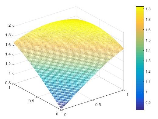
Figure 1: The numerical solution of the pressure $p_{h}^{n+1}$.

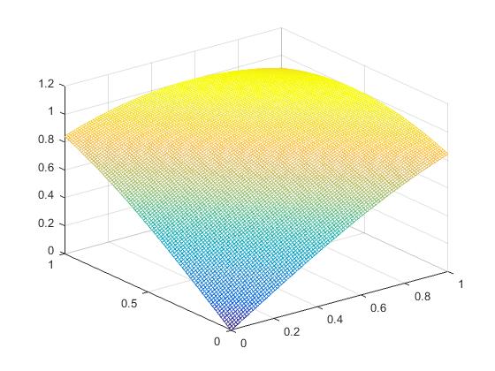
Figure 2: The analytical solution of the pressure $p$.

Figure 1 shows the numerical solution of pressure $p_{h}^{n+1}$ at $T=1$, and Figure 2 shows the analytical solution of pressure $p$. From the above figures, we can find that our method is stable and there is no “locking phenomenon”.

Test 2. Let $\Omega=[0,1]\times[0,1]$, the definition of $\Gamma_{1},\Gamma_{2},\Gamma_{3},\Gamma_{4}$ are same as Test 1, take $\Delta t=1e-6$, $T=1$. Consider the problem (2.16)-(2.18) with the following source functions:

$$\sigma(\mathbf{u})=(4-2e^{-dev(\varepsilon(\mathbf{u}))})\varepsilon(\mathbf{u})+(1+e^{-dev(\varepsilon(\mathbf{u}))}+\lambda){\mbox{\rm div\,}}\mathbf{u}I,$$

$$\mathcal{N}(\varepsilon(\mathbf{u}))=(4-2e^{-dev(\varepsilon(\mathbf{u}))})\varepsilon(\mathbf{u})+(1+e^{-dev(\varepsilon(\mathbf{u}))}){\mbox{\rm div\,}}\mathbf{u}I,$$

$$-dev(\varepsilon(\mathbf{u}))=tr(\varepsilon^{2}(\mathbf{u}))-\frac{1}{d}tr^{2}(\varepsilon(\mathbf{u})),$$

$$\phi=-\frac{c_{0}}{\pi}\sin(\pi x+\pi y)\\ +2\alpha\pi t\sin(\pi x+\pi y)-\frac{2K\pi t}{\mu_{f}}\sin(\pi x+\pi y),$$

The analytical solution of the above problem is

$$\mathbf{u} = t^{2}(\sin(\pi x)\sin(\pi y),\sin(\pi x)\sin(\pi y)),$$

$$p = -\pi^{-1}t(\sin(\pi x)\cos(\pi y)+\cos(\pi x)\sin(\pi y)).$$

The parameters are chosen as follows: $\lambda=576.923$, $\mu=384.615$, $c_{0}=0.5$, $\alpha=0.8$, $\nu=0.3$, $K=0.5$ and $E=1000$.

Table 2: Spatial errors of $\mathbf{u}$ and $p$

$h$	$\|\mathbf{u}-\mathbf{u}_{h}\|_{L^{2}(L^{2})}$	$\|\mathbf{u}-\mathbf{u}_{h}\|_{L^{2}(H^{1})}$	$\|p-p_{h}\|_{L^{2}(L^{2})}$	$\|p-p_{h}\|_{L^{2}(H^{1})}$
$h=0.176$	1.99711e-13	6.27422e-13	4.8716e-9	2.23502e-8
$h=0.088$	1.99716e-13	6.27426e-13	5.01447e-9	2.23502e-8
$h=0.044$	1.99716e-13	6.27427e-13	5.05085e-9	2.24583e-8
$h=0.022$	1.99716e-13	6.27427e-13	5.05998e-9	2.24922e-8

Table 2 displays the error of displacement $\mathbf{u}$ and the pressure $p$ with $L^{2}(0,T;$ $L^{2}(\Omega))$-norm and $L^{2}(0,T;H^{1}(\Omega))$-norm, which are consistent with the theoretical result.

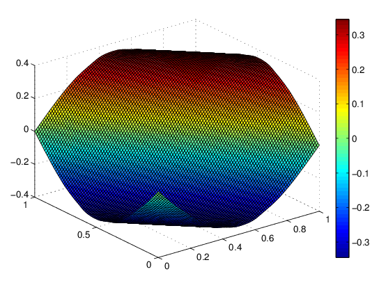
Figure 3: The analytical solution of pressure $p$ at $T$.

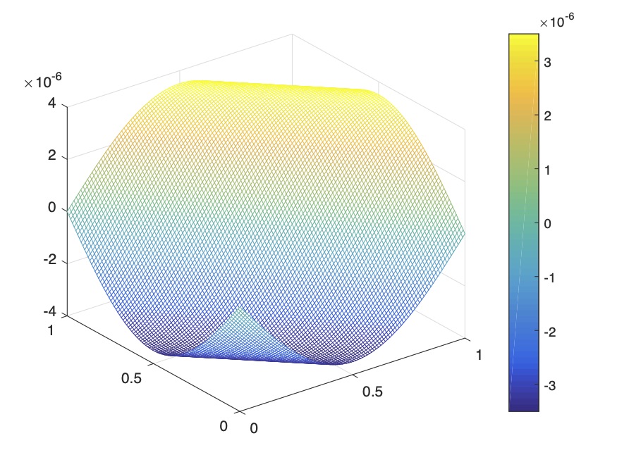
Figure 4: The numerical pressure $p_{h}^{n+1}$ at the terminal time $T$.

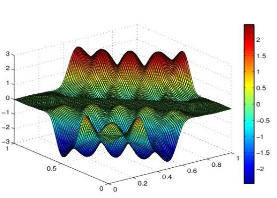
Figure 5: The pressure $p_{h}^{n+1}$ of the original problem obtained by the fully discrete algorithm.

Figure 3 shows the analytical solution of pressure $p$ at $T=1$, Figure 4 shows the numerical solution of pressure $p_{h}^{n+1}$ at $T=1$, which shows that there is no “locking” phenomenon and approximates to the true solution of pressure $p$ very well. Figure 5 shows the pressure $p_{h}^{n+1}$ solved by finite element method without multiphysics reformulation for of the original problem, which shows that there is numerical oscillation for the pressure $p$.

5 Conclusion

In this paper, we reformulate the original problem to a new coupled fluid-fluid system by using variable substitution, that is, a generalized nonlinear Stokes problem of displacement vector field related to pseudo pressure and a diffusion problem of other pseudo pressure fields. And we analyze the existence and uniqueness of the reformulated problem. A fully discrete nonlinear finite element method is proposed to solve the model numerically, that is, a multiphysics finite element method is used for the space discretization and the backward Euler method is used as the time-stepping method, the Newton method is used to solve the generalized nonlinear Stokes problem. Then, Stability analysis and the optimal order error estimates are given. Numerical tests are given to demonstrate the theoretical results, which shows that our method has no numerical oscillation. To the best of our knowledge, it is the first time to propose a fully discrete multiphysics finite element method for the nonlinear poroelasticity model with nonlinear stress-strain relations and give the optimal error estimates.

References

- [1] P.J. Phillips and M.F. Wheeler, A coupling of mixed and continuous Galerkin finite element methods for poroelasticity I: the continuous in time case. Computational Geosciences, 2007, 11(2): 131–144.
- [2] R. Showalter, Diffusion in poro-elastic media. Journal of Mathematical Analysis and Applications, 2000, 251: 310-340.
- [3] X. Feng, Z. Ge and Y. Li, Analysis of a multiphysics finite element method for a poroelasticity model. IMA Journal of Numerical Analysis, 2018, 38(1): 330-359. arXiv:1411.7464, [math.NA], 2014.
- [4] T. Roose, P.A. Netti, L.L. Munn, et al, Solid stress generated by spheroid growth estimated using a linear poroelasticity model. Microvascular Research, 2003, 66(3): 204-212.
- [5] C.C. Swan, R.S. Lakes, R.A. Brand, et al, Micromechanically based poroelastic modeling of fluid flow in haversian bone. Journal of Biomechanical Engineering-Transactions of the Asme, 2003, 125(1): 25-37.
- [6] L. Berger, A Low Order Finite Element Method for Poroelasticity with Applications to Lung Modelling. University of Oxford, 2015.
- [7] V. Luboz, A. Pedrono, et al, Prediction of tissue decompression in orbital surgery. Clinical Biomechanics, 2004, 19(2): 202-208.
- [8] M. E. Levenston, E. H. Frank and A. J. Grodzinsky, Variationally derived 3-field finite element formulations for quasistatic poroelastic analysis of hydrated biological tissues. Computer Methods in Applied Mechanics and Engineering, 1998, 156(1-4): 231-246.
- [9] D. Chapelle, J.F. Gerbeau, et al, A poroelastic model valid in large strains with applications to perfusion in cardiac modeling. Computational Mechanics, 2010, 46(1): 91 C101.
- [10] L. Berger, R. Bordas, et al, Stabilized lowest-order finite element approximation for linear three-field poroelasticity. SIAM Journal of Scientific Computing, 2015, 37(5): 2222-2245.
- [11] M. Ferronato, N. Castelletto and G. Gambolati, A fully coupled 3-D mixed finite element model of Biot consolidation. J Comput Phys, 2010, 229(12): 4813 C4830.
- [12] T. Hughes and L.P. Franca, A new finite element formulation for computational fluid dynamics: VII. The Stokes problem with various well-posed boundary conditions: symmetric formulations that converge for all velocity/pressure spaces. Computer Methods in Applied Mechanics and Engineering, 1987, 65(1): 85 C96.
- [13] J.A. White and R.I. Borja, Block-preconditioned Newton CKrylov solvers for fully coupled flow and geomechanics. Computational Geosciences, 2011, 15(4): 647 C659.
- [14] A.T. Vuong, L. Yoshihara and W.A. Wall, A general approach for modeling interacting flow through porous media under finite deformations. Computer Methods in Applied Mechanics and Engineering, 2015, 283: 1240-1259.
- [15] L. Berger, R. Bordas, D. Kay and S. Tavener, A stabilized finite element method for finite-strain three-field poroelasticity. Computational Mechanics, 2017, 60(1): 51 C68.
- [16] M.A. Murad and A. Loula, Improved accuracy in finite element analysis of Biot’s consolidation problem. Computer Methods in Applied Mechanics and Engineering, 1992, 95(3): 359-382.
- [17] M. Botti, D.A. Pietro, P. Sochala, A Hybrid High-order discretization method for nonlinear poroelasticity. Computational Methods in Applied Mathematics, 2020, 20(2): 227-249.
- [18] D. Boffi, M. Botti, D.A. Pietro, A nonconforming high-order method for the Biot problem on general meshes. SIAM Journal on Scientific Computing, 2016, 38(3): 1508-1537.
- [19] L. Bociu, G. Guidoboni, R. Sacco, J.T. Webster, Analysis of nonlinear poro-elastic and poro-visco-elastic models. Archive for Rational Mechanics and Analysis, 2016, 222(3): 1445-1519.
- [20] L. Bociu, J.T. Webster, Nonlinear quasi-static poroelasticity. Journal of Differential Equations, 2021, 296: 242-278.
- [21] Y. Cao, S. Chen, A.J. Meir, Analysis and numerical approximations of equations of nonlinear poroelasticity. Discrete and Continuous Dynamical Systems B, 2013, 18(5): 1253-1273.
- [22] Y. Cao, S. Chen, A.J. Meir, Quasilinear poroelasticity: analysis and hybrid finite element approximation. Numerical Methods for Partial Differential Equations, 2015, 31(4): 1174-1189.
- [23] C. Duijn, A. Mikelic, Mathematical Theory of Nonlinear Single Phase Poroelasticity, 2019, Preprint hal-02144933.
- [24] S. Owczarek, A Galerkin method for Biot consolidation model. Mathematics and Mechanics of Solids, 2010, 15(1): 42-56.
- [25] A. 0 5en 0 8ek, The existence and uniqueness theorem in Biot’s consolidation theory. Aplikace Matematiky, 1984, 29(3): 194-211.
- [26] S.C. Brenner and L.R. Scott, The Mathematical Theory of Finite Element Methods. Third edition, Springer, 2008.
- [27] P.G. Ciarlet, The Finite Element Method for Elliptic Problems. North-Holland, Amsterdam, 1978.
- [28] R. Temam, Navier-Stokes Equations, Studies in Mathematics and its Applications. Vol. 2, North-Holland, 1977.
- [29] S.C. Brenner, A nonconforming mixed multigrid method for the pure displacement problem in planar linear elasticity. SIAM Journal on Numerical Analysis, 1993, 30(1): 116-135.
- [30] V. Girault and P.A. Raviart, Finite Element Methods for Navier-Stokes Equations: theory and algorithms. Springer-Verlag, Berlin, Heidelberg, New York, 1980.
- [31] R. Dautray and J.L. Lions, Mathematical Analysis and Numerical Methods for Science and Technology. Vol. 1, Springer-Verlag, 1990.
- [32] M. Botti, D.A. Pietro, P. Sochala, A hybrid high-order method for nonlinear elasticity. SIAM Journal on Numerical Analysis, 2017, 55(6): 2687-2717.
- [33] L.C. Evans, Partial Differential Equations. American Mathematical Society, 2016.
- [34] F. Brezzi and M. Fortin, Mixed and Hybrid Finite Element Methods. Springer, New York, 1992.
- [35] M. Bercovier and O. Pironneau, Error estimates for finite element solution of the Stokes problem in the primitive variables. Numerische Mathematik, 1979, 33: 211-224.
- [36] X. Feng, Y. He, Fully discrete finite element approximations of a polymer gel model. SIAM Journal on Numerical Analysis, 2010, 48(6): 2186–2217.
- [37] K. Deimling, Nonlinear Functional Analysis. Berlin, Springer, 1985.