Entropy Production for
Discrete-Time Markov Processes

Abstract

We study the multiple definitions of the entropy production for discrete-time Markov processes in single systems and composite systems. We clarify the equivalence condition and the meaning of the multiple definitions and show that all definitions satisfy the important property for the entropy production, such as non-negativity. We also show that the magnitude relationship between total entropy production and marginal entropy production holds for a definition but doesn’t for another definition. Furthermore, we verify that fact by calculating entropy productions for Gaussian process and numerically illustrate the result. Finally, we find appropriate use of each definition taking all results into account.

1 Introduction

Thermodynamics deals with the equilibrium states of macroscopic systems consisting of many components (e.g., gases and liquids) and the transitions between these states. A key principle of this field is the second law of thermodynamics, which states that only processes with increasing entropy can take place in isolated systems. This principle also plays an important role in describing non-equilibrium processes in open systems that exchange heat, work, and matter with the outside world, and in closed systems where that exchange heat and work with the outside world. These systems are assumed to be in contact with the outside (the heat bath), and the concept of entropy is introduced as a measure of irreversible processes. The production of entropy is expressed as the sum of the entropy change of the system and the entropy change of the heat bath in which the system is placed, and the second law of thermodynamics is formulated in such a way that the production of entropy takes a non-negative value. For example, in both open and closed systems, the entropy of the system can be kept constant by discharging the entropy produced by irreversible processes to the heat bath and that leads to realizing non-equilibrium steady states. This sort of system forms a so-called dissipative structure, which has been proposed as a basic principle of chemical reactions and biological processes [1].

In recent years, the field of stochastic thermodynamics has evolved as a way of formulating the thermodynamic quantities of non-equilibrium processes within a framework of stochastic differential equations and information theory [2, 3, 4, 5], and nowadays, the correspondence between the second law of thermodynamics and the irreversibility of time series is clearly recognized. The entropy and heat are defined in a stochastic system based on differential equations such as the Fokker-Planck equation, which describes the probability distribution of the position of Brownian particles in a heat bath, or the master equation (which is more generalized). The entropy production is introduced as the overall change of entropy in the stochastic dynamics (entropy change of the system + entropy change of the heat bath in which the system is placed). These studies also show that entropy production is linked to the irreversibility of dynamics based on the so-called fluctuation theorem, and that the second law of thermodynamics holds at the level of expectation values as the non-negativity of entropy production.

At first, these results were limited to systems described by a single random variable (called single systems), but they have also been extended to subsystems of multiple interacting systems described by multiple random variables (called composite systems). The stochastic thermodynamics of subsystems is specifically referred to as information thermodynamics [6], and is best exemplified by Maxwell’s demon and the derivation of second-law-like limits for systems that are adaptive to time-varying environments, including living organisms [7, 8, 9, 10, 11, 12, 13, 14, 15, 16, 17, 18, 19, 20]. These results have also been verified experimentally due to advances in single-molecule manipulation techniques [21].

These advances in stochastic thermodynamics have led to the idea that entropy production is a useful indicator of irreversibility in stochastic dynamics. In recent years, it has also been applied to the stochastic dynamics of information-theoretic systems that are not in contact with a heat bath and do not exchange energy, such as neural networks [22, 23] and the analysis of time series data [24, 25].

As mentioned above, previous studies of stochastic thermodynamics have often dealt with continuous-time Markov processes based on the master equation. But stochastic thermodynamics also has important applications in discrete-time systems such as neural networks and time-series data analysis. Although entropy production is uniquely defined for continuous-time Markov processes, previous studies dealing with discrete-time processes [26, 27, 28, 29] have used multiple definitions of entropy production. This leaves several unanswered questions, including:

• How do the meanings of multiple definitions differ?

• When can multiple definitions be regarded as equivalent?

• Are these definitions consistent with their continuous-time counterparts?

• Do known inequalities—such as those derived from the decomposition of entropy production, including the second law of thermodynamics and the second law of information thermodynamics—hold for any definition?

• In a composite system, do the inequalities of entropy production for the whole system and subsystems hold?

In this paper, we aim to clarify these points regarding multiple forms of entropy production in the discrete-time Markov processes of single systems and composite systems. We confirm these results by applying them to a concrete probabilistic model. Furthermore, by taking all these results into account, we clarify the appropriate use of each definition.

This paper is organized as follows. In chapter 2, we introduce the entropy production. First, we describe the definitions of entropy production for a single system. Then, for composite systems, we present the definitions of total entropy production for an entire composite system, marginal entropy production partial entropy prodcuction, marginal entropy production, and conditional entropy production. In chapter 3, we discuss various inequalities obtained by decomposing the multiple forms of entropy production defined in chapter 2 and examining their implications. In chapter 4, we discuss the inequalities for total entropy production and marginal entropy production, and for partial entropy production and marginal entropy production. In chapter 5, as a concrete example, we calculate the total entropy production, marginal entropy production, and partial entropy production for Gaussian process, and we confirm the inequalities described in chapter 4. Chapter 6 concludes with a summary of this paper and future works.

2 Entropy Production

This chapter presents an introduction to the production of entropy, which is the subject of this research. Section 2.1 shows the multiple definitions, meanings, and properties of entropy production in discrete-time Markov processes for single systems that can be described by a single random variable. Section 2.2 shows the multiple definitions, meanings, and properties of entropy production in discrete-time Markov processes for composite systems that can be described by multiple random variables.

Although Chapters 1 to 4 deal with discrete variables to simplify the description, the same reasoning can also be applied to continuous variables by replacing the summations with integrals.

2.1 Single Systems

In this section, we examine the situation where a single system evolves over time with a discrete-time Markov process, and we discuss the definition of multiple entropy production, its properties, and its treatment in previous studies.

we will use the terminology $\mathbf{S}_{t}$ to denote a random variable representing the state of a system that varies with time $t$, $\mathbf{s}_{t}$ to denote the value of this random variable, and $P_{\mathbf{S}_{t}}(\mathbf{s}_{t})$ to denote the probability that the value of $\mathbf{S}_{t}$ is equal to $\mathbf{s}_{t}$. Similarly, in the following, we will use uppercase letters to represent random variables and lowercase letters to represent values taken by these random variables.

2.1.1 Setup

The joint probability that the state is $\mathbf{s}_{t}$ at time $t$ and $\mathbf{s}_{t+1}$ at time $t+1$ is expressed as shown below.

$$P_{\mathbf{S}_{t+1},\mathbf{S}_{t}}(\mathbf{s}_{t+1},\mathbf{s}_{t})$$ (2.1)

The probability that the state is $\mathbf{s}_{t}$ at time $t$ and the probability that the state is $\mathbf{s}_{t+1}$ at time $t+1$ are respectively obtained as follows.

$$P_{\mathbf{S}_{t}}(\mathbf{s}_{t}) =\displaystyle\sum_{\mathbf{s}_{t+1}}P_{\mathbf{S}_{t+1},\mathbf{S}_{t}}(\mathbf{s}_{t+1},\mathbf{s}_{t})$$ (2.2)

$$P_{\mathbf{S}_{t+1}}(\mathbf{s}_{t+1}) =\displaystyle\sum_{\mathbf{s}_{t}}P_{\mathbf{S}_{t+1},\mathbf{S}_{t}}(\mathbf{s}_{t+1},\mathbf{s}_{t})$$ (2.3)

These calculations are called marginalizations of $\mathbf{S}_{t+1}$ and $\mathbf{S}_{t}$ respectively, and the probability distributions obtained by the marginalization of $P_{\mathbf{S}_{t}}$ and $P_{\mathbf{S}_{t+1}}$ are called the marginal distributions of $\mathbf{S}_{t}$ and $\mathbf{S}_{t+1}$ respectively.

The conditional probability that the state is $\mathbf{s}_{t+1}$ at time $t+1$ under the condition that the state is $\mathbf{s}_{t}$ at time $t$ is expressed as follows.

$$P_{\mathbf{S}_{t+1}|\mathbf{S}_{t}}(\mathbf{s}_{t+1}|\mathbf{s}_{t})=\dfrac{P_{\mathbf{S}_{t+1},\mathbf{S}_{t}}(\mathbf{s}_{t+1},\mathbf{s}_{t})}{P_{\mathbf{S}_{t}}(\mathbf{s}_{t})}$$ (2.4)

The simultaneous probability is represented by the product of the conditional probability and the marginal distribution at time $t$.

$$P_{\mathbf{S}_{t+1},\mathbf{S}_{t}}(\mathbf{s}_{t+1},\mathbf{s}_{t})=P_{\mathbf{S}_{t+1}|\mathbf{S}_{t}}(\mathbf{s}_{t+1}|\mathbf{s}_{t})P_{\mathbf{S}_{t}}(\mathbf{s}_{t})$$ (2.5)

A process generated according to time evolution like the right side of this equation is called a forward process. Also, the conditional probability $P_{\mathbf{S}_{t+1}|\mathbf{S}_{t}}(\mathbf{s}_{t+1}|\mathbf{s}_{t})$ is called the transition probability of the forward process. A process in which the transition probability representing time evolution is represented by a conditional probability that depends only on the variables of the previous time slot is called a Markov process (Fig. 1).

Figure 1: Schematic diagram of a discrete-time Markov process in a single system.

The joint probability distribution and marginal distribution respectively satisfy the following normalization conditions.

$$\sum_{\mathbf{s}_{t+1},\mathbf{s}_{t}}P_{\mathbf{S}_{t+1},\mathbf{S}_{t}}(\mathbf{s}_{t+1},\mathbf{s}_{t}) =1,$$ (2.6)

$$\sum_{\mathbf{s}_{t}}P_{\mathbf{S}_{t}}(\mathbf{s}_{t}) =1,$$ (2.7)

$$\sum_{\mathbf{s}_{t+1}}P_{\mathbf{S}_{t+1}}(\mathbf{s}_{t+1}) =1.$$ (2.8)

In a stochastic process, a special situation can be considered in which the probability distribution does not vary over time. Under such circumstances, the system is said to be in a steady state and is defined as follows.

Definition 2.1 (Steady State).

A system is said to be in a steady state if the following relationship holds for each state $\mathbf{s}$ at arbitrary times $t,t^{\prime}$.

$$P_{\mathbf{S}_{t}}(\mathbf{s}) =P_{\mathbf{S}_{t^{\prime}}}(\mathbf{s})\quad(t\neq t^{\prime})$$ (2.9)

$$=P^{{\mathrm{ss}}}(\mathbf{s})$$ (2.10)

In this case, the probability distribution is called a stationary distribution, which is denoted by $P^{{\mathrm{ss}}}$. A process that transitions between stationary states is called a stationary process.

When a system is in a steady state, this situation can also be expressed by the balance condition defined below.

Definition 2.2 (Balance Condition).

The balance condition is given by the following relationship for any $\mathbf{s}_{t+1}$.

$$\displaystyle\sum_{\mathbf{s}_{t}}\left[{P_{\mathbf{S}_{t+1}|\mathbf{S}_{t}}(\mathbf{s}_{t+1}|\mathbf{s}_{t})P_{\mathbf{S}_{t}}(\mathbf{s}_{t})-P_{\mathbf{S}_{t+1}|\mathbf{S}_{t}}(\mathbf{s}_{t}|\mathbf{s}_{t+1})P_{\mathbf{S}_{t}}(\mathbf{s}_{t+1})}\right]=0$$ (2.11)

If the balance condition holds, this is equivalent to the system being in a steady state, as demonstrated below. First, consider the time evolution of probability.

$$P_{\mathbf{S}_{t+1}}(\mathbf{s}_{t+1})-P_{\mathbf{S}_{t}}(\mathbf{s}_{t+1}) =\displaystyle\sum_{\mathbf{s}_{t}}P_{\mathbf{S}_{t+1}|\mathbf{S}_{t}}(\mathbf{s}_{t+1}|\mathbf{s}_{t})P_{\mathbf{S}_{t}}(\mathbf{s}_{t})-P_{\mathbf{S}_{t}}(\mathbf{s}_{t+1})$$ (2.12)

$$=\displaystyle\sum_{\mathbf{s}_{t}}P_{\mathbf{S}_{t+1}|\mathbf{S}_{t}}(\mathbf{s}_{t+1}|\mathbf{s}_{t})P_{\mathbf{S}_{t}}(\mathbf{s}_{t})-\displaystyle\sum_{\mathbf{s}_{t}}P_{\mathbf{S}_{t+1}|\mathbf{S}_{t}}(\mathbf{s}_{t}|\mathbf{s}_{t+1})P_{\mathbf{S}_{t}}(\mathbf{s}_{t+1})$$ (2.13)

$$=\displaystyle\sum_{\mathbf{s}_{t}}\left[{P_{\mathbf{S}_{t+1}|\mathbf{S}_{t}}(\mathbf{s}_{t+1}|\mathbf{s}_{t})P_{\mathbf{S}_{t}}(\mathbf{s}_{t})-P_{\mathbf{S}_{t+1}|\mathbf{S}_{t}}(\mathbf{s}_{t}|\mathbf{s}_{t+1})P_{\mathbf{S}_{t}}(\mathbf{s}_{t+1})}\right]$$ (2.14)

$$=\displaystyle\sum_{\mathbf{s}_{t}}\left[{P_{\mathbf{S}_{t+1},\mathbf{S}_{t}}(\mathbf{s}_{t+1},\mathbf{s}_{t})-P_{\mathbf{S}_{t+1},\mathbf{S}_{t}}(\mathbf{s}_{t},\mathbf{s}_{t+1})}\right]$$ (2.15)

In the steady state, the left side of the equation is zero. Therefore, if the balance condition holds, this is equivalent to the system being in a steady state.

As a special case where the balance condition holds, it is possible to conceive of the following detailed balance condition where the the balance condition holds for all $\mathbf{s}_{t},\mathbf{s}_{t+1}$.

Definition 2.3 (Detailed Balance Condition).

The detailed balance condition is expressed by the following relationship for any $\mathbf{s}_{t},\mathbf{s}_{t+1}$.

$$P_{\mathbf{S}_{t+1}|\mathbf{S}_{t}}(\mathbf{s}_{t+1}|\mathbf{s}_{t})P^{{\mathrm{ss}}}(\mathbf{s}_{t}) =P_{\mathbf{S}_{t+1}|\mathbf{S}_{t}}(\mathbf{s}_{t}|\mathbf{s}_{t+1})P^{{\mathrm{ss}}}(\mathbf{s}_{t+1})$$ (2.16)

$$P_{\mathbf{S}_{t+1},\mathbf{S}_{t}}(\mathbf{s}_{t+1},\mathbf{s}_{t}) =P_{\mathbf{S}_{t+1},\mathbf{S}_{t}}(\mathbf{s}_{t},\mathbf{s}_{t+1})$$ (2.17)

When the detailed balance condition is satisfied, the system is in a special kind of steady state called the equilibrium state.

Definition 2.4 (Equilibrium State).

A system is said to be in an equilibrium state if at any time $t$ and for any $\mathbf{s}_{t+1},\mathbf{s}_{t}$, the following detailed balance condition holds.

$$P_{\mathbf{S}_{t+1}|\mathbf{S}_{t}}(\mathbf{s}_{t+1}|\mathbf{s}_{t})P^{{\mathrm{eq}}}(\mathbf{s}_{t})=P_{\mathbf{S}_{t+1}|\mathbf{S}_{t}}(\mathbf{s}_{t}|\mathbf{s}_{t+1})P^{{\mathrm{eq}}}(\mathbf{s}_{t+1})$$ (2.18)

The probability distribution at this time is called the equilibrium distribution, and is indicated by the special notation $P^{{\mathrm{eq}}}$. A process that transitions between equilibrium states is called a reversible process or an equilibrium process.

2.1.2 Backward Entropy Production

As a measure of the irreversibility of the dynamics in a stochastically varying system, it seems appropriate to use a quantity expressing how much the probability distribution representing a process differs from the probability distribution representing the same process going backwards in time. In information theory, this is defined as the Kullback–Leibler divergence (KLD), which is used in information theory as a quantity expressing the difference between two probability distributions [30].

Two definitions have been used in previous studies, which are defined here as backward entropy production and time-reversed entropy production.

Definition 2.5 (Backward Entropy Production).

Backward entropy production is defined as follows.

$$\Sigma: =\mathrm{KL}({P_{\mathbf{S}_{t:t+1}}}||{Q_{\mathbf{S}_{t:t+1}}})$$ (2.19)

$$=\sum_{\mathbf{s}_{t:t+1}}P_{\mathbf{S}_{t:t+1}}(\mathbf{s}_{t:t+1})\log\frac{P_{\mathbf{S}_{t+1}|\mathbf{S}_{t}}(\mathbf{s}_{t+1}|\mathbf{s}_{t})P_{\mathbf{S}_{t}}(\mathbf{s}_{t})}{P_{\mathbf{S}_{t+1}|\mathbf{S}_{t}}(\mathbf{s}_{t}|\mathbf{s}_{t+1})P_{\mathbf{S}_{t+1}}(\mathbf{s}_{t+1})}$$ (2.20)

where the probability distribution $Q_{\mathbf{S}_{t:t+1}}$ is given by

$$Q_{\mathbf{S}_{t:t+1}}(\mathbf{s}_{t:t+1}):=P_{\mathbf{S}_{t+1}|\mathbf{S}_{t}}(\mathbf{s}_{t}|\mathbf{s}_{t+1})P_{\mathbf{S}_{t+1}}(\mathbf{s}_{t+1})$$ (2.21)

In other words, it is a probability distribution that represents time evolution with transition probabilities complementary to those of the forward process, and with the initial distribution set to the distribution at the later time. In the following, this process is called the inverse process, and the distribution representing the inverse process is called the inverse process distribution. The probability that the values of the random variables in the transition probability of the forward process are switched in the opposite direction in time is called the transition probability of the inverse process.

When defined in this way, backward entropy production is always non-negative.

Result 2.1 (Non-Negativity of Backward Entropy Production).

Backward entropy production $\Sigma$ obeys the following rule:

$$\Sigma\geq 0.$$ (2.22)

Derivation.

This follows directly from the non-negativity of KLD [30]. Based on the conditions under which KLD is zero, this relationship becomes an equality when the following equation holds for all $\mathbf{s}_{t},\mathbf{s}_{t+1}$.

$$P_{\mathbf{S}_{t:t+1}}(\mathbf{s}_{t:t+1})=Q_{\mathbf{S}_{t:t+1}}(\mathbf{s}_{t:t+1})$$ (2.23)

From the definition of the inverse process, this can be expressed as shown below.

$$P_{\mathbf{S}_{t+1}|\mathbf{S}_{t}}(\mathbf{s}_{t+1}|\mathbf{s}_{t})P_{\mathbf{S}_{t}}(\mathbf{s}_{t}) =P_{\mathbf{S}_{t+1}|\mathbf{S}_{t}}(\mathbf{s}_{t}|\mathbf{s}_{t+1})P_{\mathbf{S}_{t+1}}(\mathbf{s}_{t+1})$$ (2.24)

$$\dfrac{P_{\mathbf{S}_{t+1},\mathbf{S}_{t}}(\mathbf{s}_{t+1},\mathbf{s}_{t})}{P_{\mathbf{S}_{t+1}}(\mathbf{s}_{t+1})} =P_{\mathbf{S}_{t+1}|\mathbf{S}_{t}}(\mathbf{s}_{t}|\mathbf{s}_{t+1})$$ (2.25)

$$P_{\mathbf{S}_{t}|\mathbf{S}_{t+1}}(\mathbf{s}_{t}|\mathbf{s}_{t+1}) =P_{\mathbf{S}_{t+1}|\mathbf{S}_{t}}(\mathbf{s}_{t}|\mathbf{s}_{t+1})$$ (2.26)

Bayes’ theorem was used to transform the second line to the third line.

From (2.26), the production of backward entropy becomes zero when the transition probability of the inverse process is equal to the posterior distribution of $\mathbf{S}_{t}$ obtained from Bayes’ theorem.

Here, when the system is in a steady state, the relationship $P_{\mathbf{S}_{t+1}}=P_{\mathbf{S}_{t}}=P^{{\mathrm{ss}}}$ can be used to rewrite this formula as

$$P_{\mathbf{S}_{t+1}|\mathbf{S}_{t}}(\mathbf{s}_{t+1}|\mathbf{s}_{t})P^{{\mathrm{ss}}}(\mathbf{s}_{t}) =P_{\mathbf{S}_{t+1}|\mathbf{S}_{t}}(\mathbf{s}_{t}|\mathbf{s}_{t+1})P^{{\mathrm{ss}}}(\mathbf{s}_{t+1})$$ (2.27)

and since (2.26) is equivalent to the detailed balance condition (2.17), its value is zero for a reversible process. ∎

2.1.3 Time-Reversed Entropy Production

Another definition of entropy production is introduced here.

Definition 2.6 (Time-Reversed Entropy Production).

Time-reversed entropy production is defined as follows.

$$\tilde{\Sigma} :=\mathrm{KL}({P_{\mathbf{S}_{t:t+1}}}||{\tilde{Q}_{\mathbf{S}_{t:t+1}}})$$ (2.28)

$$=\sum_{\mathbf{s}_{t:t+1}}P_{\mathbf{S}_{t:t+1}}(\mathbf{s}_{t:t+1})\log\frac{P_{\mathbf{S}_{t+1}|\mathbf{S}_{t}}(\mathbf{s}_{t+1}|\mathbf{s}_{t})P_{\mathbf{S}_{t}}(\mathbf{s}_{t})}{P_{\mathbf{S}_{t+1}|\mathbf{S}_{t}}(\mathbf{s}_{t}|\mathbf{s}_{t+1})P_{\mathbf{S}_{t}}(\mathbf{s}_{t+1})}$$ (2.29)

$$=\sum_{\mathbf{s}_{t:t+1}}\left[{P_{\mathbf{S}_{t+1}|\mathbf{S}_{t}}(\mathbf{s}_{t+1}|\mathbf{s}_{t})P_{\mathbf{S}_{t}}(\mathbf{s}_{t})-P_{\mathbf{S}_{t+1}|\mathbf{S}_{t}}(\mathbf{s}_{t}|\mathbf{s}_{t+1})P_{\mathbf{S}_{t}}(\mathbf{s}_{t+1})}\right]\log\frac{P_{\mathbf{S}_{t+1}|\mathbf{S}_{t}}(\mathbf{s}_{t+1}|\mathbf{s}_{t})P_{\mathbf{S}_{t}}(\mathbf{s}_{t})}{P_{\mathbf{S}_{t+1}|\mathbf{S}_{t}}(\mathbf{s}_{t}|\mathbf{s}_{t+1})P_{\mathbf{S}_{t}}(\mathbf{s}_{t+1})}$$ (2.30)

where the probability distribution $\tilde{Q}_{\mathbf{S}_{t:t+1}}$ is given by:

$$\tilde{Q}_{\mathbf{S}_{t:t+1}}(\mathbf{s}_{t:t+1}): =P_{\mathbf{S}_{t+1},\mathbf{S}_{t}}(\mathbf{s}_{t},\mathbf{s}_{t+1})$$ (2.31)

In other words, it is a probability distribution obtained by swapping the values of random variables in the forward process probability distribution to the opposite temporal direction. This sort of process is called a time-reversed process, and the resulting distribution is called a time-reversed distribution.

When defined in this way, time-reversed entropy production is always non-negative.

Result 2.2 (Non-Negativity of Time-Reversed Entropy Production).

For time-reversed entropy production $\Sigma$ the following relationship holds.

$$\tilde{\Sigma}\geq 0.$$ (2.32)

Derivation.

This follows directly from the non-negativity of KLD. Based on the conditions under which KLD is zero, this relationship becomes an equality when the following equation holds for all $\mathbf{s}_{t},\mathbf{s}_{t+1}$.

$$P_{\mathbf{S}_{t:t+1}}(\mathbf{s}_{t:t+1})=\tilde{Q}_{\mathbf{S}_{t:t+1}}(\mathbf{s}_{t:t+1})$$ (2.33)

From the definition of a time-reversed probability distribution, this can be represented as follows.

$$P_{\mathbf{S}_{t+1},\mathbf{S}_{t}}(\mathbf{s}_{t+1},\mathbf{s}_{t}) =P_{\mathbf{S}_{t+1},\mathbf{S}_{t}}(\mathbf{s}_{t},\mathbf{s}_{t+1})$$ (2.34)

$$P_{\mathbf{S}_{t+1}|\mathbf{S}_{t}}(\mathbf{s}_{t+1}|\mathbf{s}_{t})P_{\mathbf{S}_{t}}(\mathbf{s}_{t}) =P_{\mathbf{S}_{t+1}|\mathbf{S}_{t}}(\mathbf{s}_{t}|\mathbf{s}_{t+1})P_{\mathbf{S}_{t}}(\mathbf{s}_{t+1})$$ (2.35)

From (2.35), the time-reversed entropy production is zero when the detailed balance condition of (2.17) holds. ∎

2.1.4 Difference in Meaning Between Backward Entropy Production and Time-Reversed Entropy Production

The difference in meaning between backward entropy production and time-reversed entropy production is discussed below for the case where the forward process has a two-dimensional Gaussian distribution $P_{\mathbf{S}_{t+1}|\mathbf{S}_{t}}(\mathbf{s}_{t+1}|\mathbf{s}_{t})P_{\mathbf{S}_{t}}(\mathbf{s}_{t})=P_{\mathbf{S}_{t+1},\mathbf{S}_{t}}(\mathbf{s}_{t+1},\mathbf{s}_{t})$.

First, the backward entropy production is as shown in Figs. 2 and 2. In Fig. 2, the horizontal axis represents $\mathbf{S}_{t}$, the vertical axis represents $\mathbf{S}_{t+1}$, and the color map represents the value of the probability $P_{\mathbf{S}_{t+1},\mathbf{S}_{t}}(\mathbf{s}_{t+1},\mathbf{s}_{t})$. The green and red lines respectively represent the transition probability $P_{\mathbf{S}_{t+1}|\mathbf{S}_{t}}(\mathbf{s}_{t}|\mathbf{s}_{t+1})$ of the inverse process and the posterior probability $P_{\mathbf{S}_{t}|\mathbf{S}_{t+1}}(\mathbf{s}_{t}|\mathbf{s}_{t+1})$ of $\mathbf{S}_{t}$ at a specific $\mathbf{s}_{t+1}$, and the blue dotted line represents a straight line with a gradient of 1. Figure 2 shows the transition probability distribution of the inverse process and the posterior distribution of $\mathbf{S}_{t}$ arranged with $\mathbf{s}_{t}$ as a variable, and the green and red dots show the pair of values corresponding to a specific $\mathbf{s}_{t}$. Since backward entropy production is a quantity that compares the green and red dots in Fig. 2, the difference between the posterior distribution of ${S}_{t}$ and the transition probability of the inverse process is expressed by Bayesian inference. In this case, if the distribution of $\mathbf{S}_{t}$ obtained according to the transition probability of the forward process starting from $\mathbf{S}_{t+1}$ is equivalent to performing Bayesian inference, then the backward entropy production will be zero. In other words, when the forward evolution of a temporal series is equivalent to making Bayesian optimal inferences about past states, this discrete process is defined as a process with no temporal directionality, so backward entropy production is a quantified measure of deviation from this sort of process.

Next, time-reversed entropy production is shown in Fig. 3, where the horizontal axis represents $\mathbf{S}_{t}$, the vertical axis represents $\mathbf{S}_{t+1}$, and the color map represents the values of the probabilities $P_{\mathbf{S}_{t+1},\mathbf{S}_{t}}(\mathbf{s}_{t+1},\mathbf{s}_{t})$. With regard to the blue dotted line with a gradient of 1, the symmetrical green and red dots represent $P_{\mathbf{S}_{t+1},\mathbf{S}_{t}}(\mathbf{s}_{t+1},\mathbf{s}_{t})$ and $P_{\mathbf{S}_{t+1},\mathbf{S}_{t}}(\mathbf{s}_{t},\mathbf{s}_{t+1})$ for a particular $\mathbf{s}_{t+1},\mathbf{s}_{t}$, respectively. Time-reversed entropy production is a quantity that compares the green and red points in Fig. 3, and $P_{\mathbf{S}_{t+1},\mathbf{S}_{t}}(\mathbf{s}_{t+1},\mathbf{s}_{t})=P_{\mathbf{S}_{t+1},\mathbf{S}_{t}}(\mathbf{s}_{t},\mathbf{s}_{t+1})$ is equivalent to the detailed balance condition (2.17), which represents the degree of violation of the detailed balance. In other words, it can be regarded as a measure of the irreversibility of non-equilibrium stochastic dynamics.

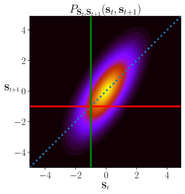
(a)

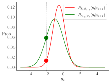
(b)

Figure 2: Backward entropy production in a two-dimensional Gaussian distribution. (a) Transition probability of the inverse process $P_{\mathbf{S}_{t+1}|\mathbf{S}_{t}}(\mathbf{s}_{t}|\mathbf{s}_{t+1})$ in a two-dimensional Gaussian distribution and posterior probability $P_{\mathbf{S}_{t}|\mathbf{S}_{t+1}}(\mathbf{s}_{t}|\mathbf{s}_{t+1})$ of $\mathbf{S}_{t}$; (b) These probabilities expressed as functions of the same variable $\mathbf{s}_{t}$

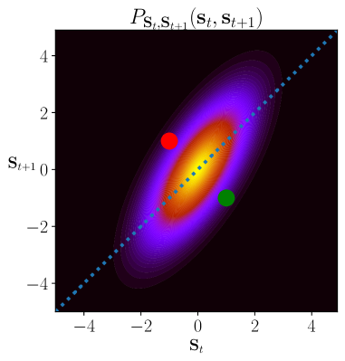
Figure 3: Time-reversed entropy production in a two-dimensional Gaussian distribution.

2.1.5 Relationship Between Backward Entropy Production and Time-Reversed Entropy Production

Conditions for equivalence

Under certain conditions, the backward entropy production and time-reversed entropy production defined above are equivalent. To start with, the difference between the two can be expressed as follows.

$$\tilde{\Sigma}-\Sigma =\mathrm{KL}({P_{\mathbf{S}_{t:t+1}}}||{\tilde{Q}_{\mathbf{S}_{t:t+1}}})-\mathrm{KL}({P_{\mathbf{S}_{t:t+1}}}||{Q_{\mathbf{S}_{t:t+1}}})$$ (2.36)

$$=\mathbb{E}_{\mathbf{S}_{t:t+1}}\left[{\log\dfrac{Q_{\mathbf{S}_{t:t+1}}}{\tilde{Q}_{\mathbf{S}_{t:t+1}}}}\right]$$ (2.37)

$$=\sum_{\mathbf{s}}P_{\mathbf{S}_{t+1}}(\mathbf{s})\log\dfrac{P_{\mathbf{S}_{t+1}}(\mathbf{s})}{P_{\mathbf{S}_{t}}(\mathbf{s})}$$ (2.38)

$$=\mathrm{KL}({P_{\mathbf{S}_{t+1}}}||{P_{\mathbf{S}_{t}}})$$ (2.39)

Therefore, the following relationship holds:

Result 2.3 (Magnitude relationship between Backward Entropy Production and Time-Reversed Entropy Production).

The following inequality holds between backward entropy production and time-reversed entropy production:

$$\tilde{\Sigma}\geq\Sigma.$$ (2.40)

Derivation.

This holds because $\tilde{\Sigma}-\Sigma=\mathrm{KL}({P_{\mathbf{S}_{t+1}}}||{P_{\mathbf{S}_{t}}})$ and due to the non-negativity of KLD. When equality holds, i.e., under conditions where the backward entropy production and time-reversed entropy production are equivalent, the equality $P_{\mathbf{S}_{t+1}}(\mathbf{s})=P_{\mathbf{S}_{t}}(\mathbf{s})$ holds for any $\mathbf{s}$. In other words, in the steady state, backward entropy production and time-reversed entropy production are equivalent. ∎

Continuous-time limit

These definitions are also equivalent when considering the continuum limit with regard to time. If time is a continuous variable in $\tilde{\Sigma}-\Sigma=\mathrm{KL}({P_{\mathbf{S}_{t+1}}}||{P_{\mathbf{S}_{t}}})$ and is discretized by a time interval $\tau$, it can be expanded as follows.

$$\mathrm{KL}({P_{\mathbf{S}_{t+\tau}}}||{P_{\mathbf{S}_{t}}})$$ (2.41)

$$=\sum_{\mathbf{s}}P_{\mathbf{S}_{t+\tau}}(\mathbf{s})\log\dfrac{P_{\mathbf{S}_{t+\tau}}(\mathbf{s})}{P_{\mathbf{S}_{t}}(\mathbf{s})}$$ (2.42)

$$=\sum_{\mathbf{s}}P_{\mathbf{S}_{t+\tau}}(\mathbf{s})\log\dfrac{P_{\mathbf{S}_{t}}(\mathbf{s})+\tau\dfrac{\partial{P_{\mathbf{S}_{t}}(\mathbf{s})}}{\partial{t}}+\dfrac{\tau^{2}}{2}\dfrac{\partial^{2}{P_{\mathbf{S}_{t}}(\mathbf{s})}}{\partial{t}^{2}}+O(\tau^{3})}{P_{\mathbf{S}_{t}}(\mathbf{s})}$$ (2.43)

$$=\sum_{\mathbf{s}}P_{\mathbf{S}_{t+\tau}}(\mathbf{s})\log\left({1+\tau\dfrac{1}{P_{\mathbf{S}_{t}}(\mathbf{s})}\dfrac{\partial{P_{\mathbf{S}_{t}}(\mathbf{s})}}{\partial{t}}+\dfrac{\tau^{2}}{2}\dfrac{1}{P_{\mathbf{S}_{t}}(\mathbf{s})}\dfrac{\partial^{2}{P_{\mathbf{S}_{t}}(\mathbf{s})}}{\partial{t}^{2}}+O(\tau^{3})}\right)$$ (2.44)

$$=\sum_{\mathbf{s}}\left({P_{\mathbf{S}_{t}}(\mathbf{s})+\tau\dfrac{\partial{P_{\mathbf{S}_{t}}(\mathbf{s})}}{\partial{t}}+O(\tau^{2})}\right)\left({\tau\dfrac{1}{P_{\mathbf{S}_{t}}(\mathbf{s})}\dfrac{\partial{P_{\mathbf{S}_{t}}(\mathbf{s})}}{\partial{t}}+\dfrac{\tau^{2}}{2}\dfrac{1}{P_{\mathbf{S}_{t}}(\mathbf{s})}\dfrac{\partial^{2}{P_{\mathbf{S}_{t}}(\mathbf{s})}}{\partial{t}^{2}}+O(\tau^{3})}\right)$$ (2.45)

$$=\sum_{\mathbf{s}}\left({\tau\dfrac{\partial{P_{\mathbf{S}_{t}}(\mathbf{s})}}{\partial{t}}+\dfrac{\tau^{2}}{2}\dfrac{\partial^{2}{P_{\mathbf{S}_{t}}(\mathbf{s})}}{\partial{t}^{2}}+\tau^{2}\dfrac{1}{P_{\mathbf{S}_{t}}(\mathbf{s})}\dfrac{\partial^{2}{P_{\mathbf{S}_{t}}(\mathbf{s})}}{\partial{t}^{2}}+O(\tau^{3})}\right)$$ (2.46)

$$=\sum_{\mathbf{s}}\tau^{2}\dfrac{1}{P_{\mathbf{S}_{t}}(\mathbf{s})}\dfrac{\partial^{2}{P_{\mathbf{S}_{t}}(\mathbf{s})}}{\partial{t}^{2}}+O(\tau^{3})$$ (2.47)

$$=O(\tau^{2})$$ (2.48)

where the seventh line is obtained from the sixth by applying the normalization condition $\sum_{\mathbf{s}}P_{\mathbf{S}_{t}}(\mathbf{s})=1$. Therefore, this becomes zero at the continuum limit $\tau\rightarrow 0$.

2.1.6 Previous Studies

Previous studies focused on either backward entropy production or time-reversed entropy production in discrete-time systems as summarized below. These are both identical at the continuum limit, but when a continuous-time stochastic process is discretized with a certain time interval, its definition is taken to be the definition in discrete time.

Table 1: Treatment of entropy production in previous studies

Type of entropy production handled	Major previous studies
Backward: $\Sigma$	Lee (2018), Ito et al. (2020), Liu et al. (2020)
Time-Reversed: $\tilde{\Sigma}$	Gaspard (2004), Touchette (2009), Proesmans et al. (2017)

2.2 Composite Systems

In this section, we present multiple definitions of entropy for a composite system XY consisting of two interacting systems X and Y that evolve in time as a whole based on a discrete-time Markov process, and we discuss the properties of such systems and their treatment in previous studies.

2.2.1 Setup

The random variables representing the state of systems X and Y at time $t$ are $\mathbf{X}_{t}$ and $\mathbf{Y}_{t}$, respectively. By setting $\mathbf{S}_{t}=\left\{{\mathbf{X}_{t},\mathbf{Y}_{t}}\right\}$ in section 2.1, the probability distribution representing the process from time $t$ to $t+1$ is defined in the same way. The steady state (2.10), the balance condition (2.11), the detailed balance condition (2.17), and the equilibrium state (2.18) are also defined in the same way. In particular, the detailed balance of a composite system can be expressed as follows.

Definition 2.7 (Detailed Balance Condition of a Composite System).

The detailed balance condition in a composite system is expressed by the following relation for any $\mathbf{x}_{t},\mathbf{y}_{t},\mathbf{x}_{t+1},\mathbf{y}_{t+1}$.

$$P_{\mathbf{X}_{t+1},\mathbf{Y}_{t+1}|\mathbf{X}_{t},\mathbf{Y}_{t}}(\mathbf{x}_{t+1},\mathbf{y}_{t+1}|\mathbf{x}_{t},\mathbf{y}_{t})P_{\mathbf{X}_{t},\mathbf{Y}_{t}}(\mathbf{x}_{t},\mathbf{y}_{t}) =P_{\mathbf{X}_{t+1},\mathbf{Y}_{t+1}|\mathbf{X}_{t},\mathbf{Y}_{t}}(\mathbf{x}_{t},\mathbf{y}_{t}|\mathbf{x}_{t+1},\mathbf{y}_{t+1})P_{\mathbf{X}_{t},\mathbf{Y}_{t}}(\mathbf{x}_{t+1},\mathbf{y}_{t+1})$$ (2.49)

In addition, stochastic thermodynamics often requires that the time evolution of composite system XY is bipartite [14, 15, 18, 17, 16, 9, 19, 10, 13, 28, 8, 11]. Bipartiteness is the property whereby, given the current values of X and Y, the next values of X and Y are conditionally independent, indicating that the time evolution of the composite system XY can be divided into separate time evolutions for X and Y.

Definition 2.8 (Bipartiteness).

For any $\mathbf{x}_{t},\mathbf{y}_{t},\mathbf{x}_{t+1},\mathbf{y}_{t+1}$, the property of bipartiteness is expressed as follows.

$$P_{\mathbf{X}_{t+1},\mathbf{Y}_{t+1}|\mathbf{X}_{t},\mathbf{Y}_{t}}(\mathbf{x}_{t+1},\mathbf{y}_{t+1}|\mathbf{x}_{t},\mathbf{y}_{t})=P_{\mathbf{X}_{t+1}|\mathbf{X}_{t},\mathbf{Y}_{t}}(\mathbf{x}_{t+1}|\mathbf{x}_{t},\mathbf{y}_{t})P_{\mathbf{Y}_{t+1}|\mathbf{X}_{t},\mathbf{Y}_{t}}(\mathbf{y}_{t+1}|\mathbf{x}_{t},\mathbf{y}_{t})$$ (2.50)

This section presents a more general examination of the time evolution of non-bipartite composite systems that do not satisfy bipartiteness [31, 25, 32] (Fig. 4). In other words, the time evolution of a subsystem X(Y) is described by the conditional probability distribution $P_{\mathbf{X}_{t+1}|\mathbf{Y}_{t+1},\mathbf{X}_{t},\mathbf{Y}_{t}}(P_{\mathbf{Y}_{t+1}|\mathbf{Y}_{t+1},\mathbf{X}_{t},\mathbf{Y}_{t}})$.

Figure 4: Schematic diagram of a discrete-time Markov process in a composite system.

2.2.2 Total Entropy Production

In backward entropy production (2.19) and time-reversed entropy production (2.28) as described in section 2.1, the entropy production of the entire composite system can be defined by setting $\mathbf{S}_{t}=\left\{{\mathbf{X}_{t},\mathbf{Y}_{t}}\right\}$. This is called the total entropy production, which has two definitions based on backward total entropy production and time-reversed total entropy production. In the same way as for a single system, it is possible to show that the entropy production is non-negative in both cases.

Definition 2.9 (Backward total entropy production).

$$\Sigma_{{\mathrm{XY}}}^{{\mathrm{tot}}}:=\mathrm{KL}({P_{\mathbf{X}_{t:t+1},\mathbf{Y}_{t:t+1}}}||{Q_{\mathbf{X}_{t:t+1},\mathbf{Y}_{t:t+1}}})$$ (2.51)

where is $Q_{\mathbf{X}_{t:t+1},\mathbf{Y}_{t:t+1}}$ is defined as follows.

$$Q_{\mathbf{X}_{t:t+1},\mathbf{Y}_{t:t+1}}(\mathbf{x}_{t:t+1},\mathbf{y}_{t:t+1}):=P_{\mathbf{X}_{t+1},\mathbf{Y}_{t+1}|\mathbf{X}_{t},\mathbf{Y}_{t}}(\mathbf{x}_{t},\mathbf{y}_{t}|\mathbf{x}_{t+1},\mathbf{y}_{t+1})P_{\mathbf{X}_{t+1},\mathbf{Y}_{t+1}}(\mathbf{x}_{t+1},\mathbf{y}_{t+1})$$ (2.52)

In other words, it is a probability distribution that represents time evolution based on transition probabilities in the opposite direction to the forward process, with the initial distribution set to the distribution at the later time. This sort of process is called the inverse process of the composite system, and the distribution of an inverse process is called an inverse process distribution.

Definition 2.10 (Time-Reversed Total Entropy Production).

$$\tilde{\Sigma}_{{\mathrm{XY}}}^{{\mathrm{tot}}}:=\mathrm{KL}({P_{\mathbf{X}_{t:t+1},\mathbf{Y}_{t:t+1}}}||{\tilde{Q}_{\mathbf{X}_{t:t+1},\mathbf{Y}_{t:t+1}}})$$ (2.53)

where $\tilde{Q}_{\mathbf{X}_{t:t+1},\mathbf{Y}_{t:t+1}}$ is defined as follows:

$$\tilde{Q}_{\mathbf{X}_{t:t+1},\mathbf{Y}_{t:t+1}}(\mathbf{x}_{t:t+1},\mathbf{y}_{t:t+1}):= P_{\mathbf{X}_{t+1},\mathbf{Y}_{t+1}|\mathbf{X}_{t},\mathbf{Y}_{t}}(\mathbf{x}_{t},\mathbf{y}_{t}|\mathbf{x}_{t+1},\mathbf{y}_{t+1})P_{\mathbf{X}_{t},\mathbf{Y}_{t}}(\mathbf{x}_{t+1},\mathbf{y}_{t+1})$$ (2.54)

$$= P_{\mathbf{X}_{t+1},\mathbf{Y}_{t+1},\mathbf{X}_{t},\mathbf{Y}_{t}}(\mathbf{x}_{t},\mathbf{y}_{t},\mathbf{x}_{t+1},\mathbf{y}_{t+1})$$ (2.55)

In other words, it is a probability distribution obtained by swapping the values of random variables in the forward process probability distribution to the opposite temporal direction. This sort of process is called a composite system time-reversed process, and the resulting distribution is called a time-reversed distribution.

For both definitions of total entropy production, the production of entropy is non-negative as in the case of a single system.

Result 2.4 (Non-Negativity of Total Entropy Production).

For backward total entropy production, $\Sigma_{{\mathrm{XY}}}^{{\mathrm{tot}}}$ and time-reversed total entropy production $\tilde{\Sigma}_{{\mathrm{XY}}}^{{\mathrm{tot}}}$,

$$\Sigma_{{\mathrm{XY}}}^{{\mathrm{tot}}} \geq 0,$$ (2.56)

$$\tilde{\Sigma}_{{\mathrm{XY}}}^{{\mathrm{tot}}} \geq 0.$$ (2.57)

Derivation.

This follows directly from the non-negativity of KLD. Based on the conditions under which KLD is zero, this relationship becomes an equality in the case of backward entropy production when the following condition holds for all $\mathbf{x}_{t},\mathbf{y}_{t},\mathbf{x}_{t+1},\mathbf{y}_{t+1}$:

$$P_{\mathbf{X}_{t:t+1},\mathbf{Y}_{t:t+1}}(\mathbf{x}_{t:t+1},\mathbf{y}_{t:t+1})=Q_{\mathbf{X}_{t:t+1},\mathbf{Y}_{t:t+1}}(\mathbf{x}_{t:t+1},\mathbf{y}_{t:t+1})$$ (2.58)

As in (2.26), this results in the following relationship:

$$P_{\mathbf{X}_{t},\mathbf{Y}_{t}|\mathbf{X}_{t+1},\mathbf{Y}_{t+1}}(\mathbf{x}_{t},\mathbf{y}_{t}|\mathbf{x}_{t+1},\mathbf{y}_{t+1}) =P_{\mathbf{X}_{t+1},\mathbf{Y}_{t+1}|\mathbf{X}_{t},\mathbf{Y}_{t}}(\mathbf{x}_{t},\mathbf{y}_{t}|\mathbf{x}_{t+1},\mathbf{y}_{t+1})$$ (2.59)

In other words, backward total entropy production expresses the difference between the distribution representing the forward process of the composite system and the distribution of the backward process in which the initial distribution is set at time $t+1$ and the state transition occurs in the opposite direction from the forward process.

For the time-reversed case, the following relationship holds for all $\mathbf{x}_{t},\mathbf{y}_{t},\mathbf{x}_{t+1},\mathbf{y}_{t+1}$:

$$P_{\mathbf{X}_{t:t+1},\mathbf{Y}_{t:t+1}}(\mathbf{x}_{t:t+1},\mathbf{y}_{t:t+1})=\tilde{Q}_{\mathbf{X}_{t:t+1},\mathbf{Y}_{t:t+1}}(\mathbf{x}_{t:t+1},\mathbf{y}_{t:t+1})$$ (2.60)

As in (2.35), this results in the following relationship:

$$P_{\mathbf{X}_{t+1},\mathbf{Y}_{t+1}|\mathbf{X}_{t},\mathbf{Y}_{t}}(\mathbf{x}_{t+1},\mathbf{y}_{t+1}|\mathbf{x}_{t},\mathbf{y}_{t})P_{\mathbf{X}_{t},\mathbf{Y}_{t}}(\mathbf{x}_{t},\mathbf{y}_{t}) =P_{\mathbf{X}_{t+1},\mathbf{Y}_{t+1}|\mathbf{X}_{t},\mathbf{Y}_{t}}(\mathbf{x}_{t},\mathbf{y}_{t}|\mathbf{x}_{t+1},\mathbf{y}_{t+1})P_{\mathbf{X}_{t},\mathbf{Y}_{t}}(\mathbf{x}_{t+1},\mathbf{y}_{t+1})$$ (2.61)

which becomes zero in a reversible process where the detailed balance condition (2.49) holds. In other words, time-reversed total entropy production represents the degree to which the detailed balance of the composite system is violated. ∎

2.2.3 Partial Entropy Production

Partial entropy production can be defined for a subsystem X that forms part of a composite system XY (and can also be defined for Y by swapping the random variables of X and Y). As with total entropy production, two types of partial entropy can be defined: backward partial entropy production and time-reversed partial entropy production.

Definition 2.11 (Backward Partial Entropy Production).

$$\Sigma_{{\mathrm{X}}}^{\mathrm{par}}:=\mathrm{KL}({P_{\mathbf{X}_{t:t+1},\mathbf{Y}_{t:t+1}}}||{Q_{\mathbf{X}_{t:t+1},\mathbf{Y}_{t:t+1}}^{\mathrm{par}}})$$ (2.62)

where $Q_{\mathbf{X}_{t:t+1},\mathbf{Y}_{t:t+1}}^{{\mathrm{par}}}$ is defined as:

$$Q_{\mathbf{X}_{t:t+1},\mathbf{Y}_{t:t+1}}^{\mathrm{par}}(\mathbf{x}_{t:t+1},\mathbf{y}_{t:t+1}):=P_{\mathbf{X}_{t+1}|\mathbf{Y}_{t+1},\mathbf{X}_{t},\mathbf{Y}_{t}}(\mathbf{x}_{t}|\mathbf{y}_{t},\mathbf{x}_{t+1},\mathbf{y}_{t+1})P_{\mathbf{X}_{t+1},\mathbf{Y}_{t+1},\mathbf{Y}_{t}}(\mathbf{x}_{t+1},\mathbf{y}_{t+1},\mathbf{y}_{t})$$ (2.63)

That is to say, it is a probability distribution that represents a process where state transitions in the opposite direction to the forward process occur in the time evolution of subsystem X when given the value of X at the later time and Y at times $t$ and $t+1$. This sort of process is called a partial inverse process of X, and the distribution of a partial inverse process is called a partial inverse process distribution.

Definition 2.12 (Time-Reversed Partial Entropy Production).

$$\tilde{\Sigma}_{{\mathrm{X}}}^{\mathrm{par}}:=\mathrm{KL}({P_{\mathbf{X}_{t:t+1},\mathbf{Y}_{t:t+1}}}||{\tilde{Q}_{\mathbf{X}_{t:t+1},\mathbf{Y}_{t:t+1}}^{{\mathrm{par}}}})$$ (2.64)

where $\tilde{Q}_{\mathbf{X}_{t:t+1},\mathbf{Y}_{t:t+1}}^{{\mathrm{par}}}$ is defined as follows:

$$\tilde{Q}_{\mathbf{X}_{t:t+1},\mathbf{Y}_{t:t+1}}^{{\mathrm{par}}}(\mathbf{x}_{t:t+1},\mathbf{y}_{t:t+1}):= P_{\mathbf{X}_{t+1}|\mathbf{Y}_{t+1},\mathbf{X}_{t},\mathbf{Y}_{t}}(\mathbf{x}_{t}|\mathbf{y}_{t+1},\mathbf{x}_{t+1},\mathbf{y}_{t})P_{\mathbf{X}_{t},\mathbf{Y}_{t+1},\mathbf{Y}_{t}}(\mathbf{x}_{t+1},\mathbf{y}_{t+1},\mathbf{y}_{t})$$ (2.65)

$$= P_{\mathbf{X}_{t+1},\mathbf{Y}_{t+1},\mathbf{X}_{t},\mathbf{Y}_{t}}(\mathbf{x}_{t},\mathbf{y}_{t+1},\mathbf{x}_{t+1},\mathbf{y}_{t})$$ (2.66)

In other words, it is a probability distribution obtained by swapping only the values of subsystem X in the forward process probability distribution to the opposite temporal direction. This sort of process is called a partial time-reversed process, and the distribution of a partial time-reversed process is called a partial time-reversed distribution.

For these forms of partial entropy production, the non-negativity property holds.

Result 2.5 (Non-Negativity of Partial Entropy Production).

For backward partial entropy production $\Sigma_{{\mathrm{X}}}^{{\mathrm{par}}}$ and time-reversed partial entropy production $\tilde{\Sigma}_{{\mathrm{X}}}^{{\mathrm{par}}}$,

$$\Sigma_{{\mathrm{X}}}^{\mathrm{par}} \geq 0,$$ (2.67)

$$\tilde{\Sigma}_{{\mathrm{X}}}^{\mathrm{par}} \geq 0.$$ (2.68)

Derivation.

This follows directly from the non-negativity of KLD. Based on the conditions under which KLD is zero, this relationship becomes an equality in the case of backward entropy production when the following condition holds for all $\mathbf{x}_{t},\mathbf{y}_{t},\mathbf{x}_{t+1},\mathbf{y}_{t+1}$:

$$P_{\mathbf{X}_{t:t+1},\mathbf{Y}_{t:t+1}}(\mathbf{x}_{t:t+1}.\mathbf{y}_{t:t+1})=Q_{\mathbf{X}_{t:t+1},\mathbf{Y}_{t:t+1}}^{\mathrm{par}}(\mathbf{x}_{t:t+1},\mathbf{y}_{t:t+1}).$$ (2.69)

In other words, backward partial entropy production expresses the difference between the distribution of the forward process and the distribution of the process in which state transitions occur in the opposite direction to the forward processes in the time evolution of subsystem X, given X at the later time and Y at times $t$ and $t+1$.

For the time-reversed case, the following relationship holds for all $\mathbf{x}_{t},\mathbf{y}_{t},\mathbf{x}_{t+1},\mathbf{y}_{t+1}$:

$$P_{\mathbf{X}_{t:t+1}.\mathbf{Y}_{t:t+1}}(\mathbf{x}_{t:t+1},\mathbf{y}_{t:t+1})=\tilde{Q}_{\mathbf{X}_{t:t+1},\mathbf{Y}_{t:t+1}}^{{\mathrm{par}}}(\mathbf{x}_{t:t+1},\mathbf{y}_{t:t+1})$$ (2.70)

In other words, time-reversed entropy production expresses the difference between the distribution of the forward process and the distribution of the process in which only X performs state transitions in the opposite direction to the forward process. ∎

2.2.4 Marginal Entropy Production

Marginal entropy production can be defined using the marginal distribution of X obtained by summing the joint distributions of X and Y for the constituent part X of a composite system XY. (By exchanging the random variables X and Y, the marginal entropy production of Y can also be defined in the same way.

Definition 2.13 (Backward Marginal Entropy Production).

$$\Sigma_{{\mathrm{X}}}^{\mathrm{mar}}:=\mathrm{KL}({P_{\mathbf{X}_{t:t+1}}}||{Q^{{\mathrm{mar}}}_{\mathbf{X}_{t:t+1}}})$$ (2.71)

where $P_{\mathbf{X}_{t:t+1}}(\mathbf{x}_{t:t+1})$ is obtained by marginalizing $P_{\mathbf{X}_{t:t+1},\mathbf{Y}_{t:t+1}}(\mathbf{x}_{t:t+1},\mathbf{y}_{t:t+1})$ with respect to Y.

$$P_{\mathbf{X}_{t:t+1}}(\mathbf{x}_{t:t+1}) =\displaystyle\sum_{\mathbf{y}_{t:t+1}}P_{\mathbf{X}_{t:t+1},\mathbf{Y}_{t:t+1}}(\mathbf{x}_{t:t+1},\mathbf{y}_{t:t+1})$$ (2.72)

Unlike the marginalization of $Q_{\mathbf{X}_{t:t+1},\mathbf{Y}_{t:t+1}}(\mathbf{x}_{t:t+1},\mathbf{y}_{t:t+1})$ with respect to Y, $Q^{{\mathrm{mar}}}_{\mathbf{X}_{t:t+1}}$ is defined separately as follows:

$$Q^{{\mathrm{mar}}}_{\mathbf{X}_{t:t+1}}(\mathbf{x}_{t:t+1}) =P_{\mathbf{X}_{t+1}|\mathbf{X}_{t}}(\mathbf{x}_{t}|\mathbf{x}_{t+1})P_{\mathbf{X}_{t+1}}(\mathbf{x}_{t+1})$$ (2.73)

$$\neq\displaystyle\sum_{\mathbf{y}_{t:t+1}}Q_{\mathbf{X}_{t:t+1},\mathbf{Y}_{t:t+1}}(\mathbf{x}_{t:t+1},\mathbf{y}_{t:t+1})$$ (2.74)

In the marginal distribution of X, this is a probability distribution that represents time evolution based on transition probabilities in the opposite direction to the forward process, with the initial distribution set to the distribution at the later time. This sort of process is called a marginal inverse process, and a distribution of marginal inverse processes is called a marginal inverse process distribution.

Definition 2.14 (Time-Reversed Marginal Entropy Production).

$$\tilde{\Sigma}_{{\mathrm{X}}}^{\mathrm{mar}}:=\mathrm{KL}({P_{\mathbf{X}_{t:t+1}}}||{\tilde{Q}^{{\mathrm{mar}}}_{\mathbf{X}_{t:t+1}}})$$ (2.75)

where $P_{\mathbf{X}_{t:t+1}}(\mathbf{x}_{t:t+1})$ is obtained by marginalizing $P_{\mathbf{X}_{t:t+1},\mathbf{Y}_{t:t+1}}(\mathbf{x}_{t:t+1},\mathbf{y}_{t:t+1})$ with respect to Y, and $\tilde{Q}^{{\mathrm{mar}}}_{\mathbf{X}_{t:t+1}}(\mathbf{x}_{t:t+1})$ is also obtained by marginalizing $\tilde{Q}_{\mathbf{X}_{t:t+1},\mathbf{Y}_{t:t+1}}(\mathbf{x}_{t:t+1},\mathbf{y}_{t:t+1})$ with respect to Y.

$$P_{\mathbf{X}_{t:t+1}}(\mathbf{x}_{t:t+1}) =\displaystyle\sum_{\mathbf{y}_{t:t+1}}P_{\mathbf{X}_{t:t+1},\mathbf{Y}_{t:t+1}}(\mathbf{x}_{t:t+1},\mathbf{y}_{t:t+1})$$ (2.76)

$$\tilde{Q}^{{\mathrm{mar}}}_{\mathbf{X}_{t:t+1}}(\mathbf{x}_{t:t+1}) =\displaystyle\sum_{\mathbf{y}_{t:t+1}}\tilde{Q}_{\mathbf{X}_{t:t+1},\mathbf{Y}_{t:t+1}}(\mathbf{x}_{t:t+1},\mathbf{y}_{t:t+1})$$ (2.77)

$$=\tilde{Q}_{\mathbf{X}_{t:t+1}}(\mathbf{x}_{t:t+1})$$ (2.78)

$$=P_{\mathbf{X}_{t+1},\mathbf{X}_{t}}(\mathbf{x}_{t},\mathbf{x}_{t+1})$$ (2.79)

In other words, in a marginal distribution, this is the probability distribution obtained by swapping the values of random variables in the forward process probability distribution to the opposite temporal direction. This sort of process is called a marginal time-reversed process, and the resulting marginal distribution is called a marginal time-reversed distribution.

For these forms of marginal entropy production, the non-negativity property holds.

Result 2.6 (Non-Negativity of Marginal Entropy Production).

For backward marginal entropy production $\Sigma_{{\mathrm{X}}}^{{\mathrm{mar}}}$ and time-reversed marginal entropy production $\tilde{\Sigma}_{{\mathrm{X}}}^{{\mathrm{mar}}}$,

$$\Sigma_{{\mathrm{X}}}^{\mathrm{mar}} \geq 0,$$ (2.80)

$$\tilde{\Sigma}_{{\mathrm{X}}}^{\mathrm{mar}} \geq 0.$$ (2.81)

Derivation.

This follows directly from the non-negativity of KLD. Based on the conditions under which KLD is zero, this relationship becomes an equality in the case of backward entropy production when the following condition holds for all $\mathbf{x}_{t},\mathbf{x}_{t+1}$.

$$P_{\mathbf{X}_{t:t+1}}(\mathbf{x}_{t},\mathbf{x}_{t+1})=Q_{\mathbf{X}_{t:t+1}}(\mathbf{x}_{t},\mathbf{x}_{t+1})$$ (2.82)

In other words, backward marginal entropy production expresses the difference between the distribution representing the marginalized forward process of X and the distribution of the process whereby state transitions occur in the opposite direction from the forward process in the marginal distribution of X where the initial distribution is set at time $t+1$. In the time-reversed case, the following condition holds for all $\mathbf{x}_{t},\mathbf{x}_{t+1}$.

$$P_{\mathbf{X}_{t:t+1}}(\mathbf{x}_{t},\mathbf{x}_{t+1})=\tilde{Q}_{\mathbf{X}_{t:t+1}}(\mathbf{x}_{t},\mathbf{x}_{t+1})$$ (2.83)

This means that

$$P_{\mathbf{X}_{t+1},|\mathbf{X}_{t},}(\mathbf{x}_{t+1}|\mathbf{x}_{t})P_{\mathbf{X}_{t}}(\mathbf{x}_{t}) =P_{\mathbf{X}_{t+1}|\mathbf{X}_{t}}(\mathbf{x}_{t}|\mathbf{x}_{t+1})P_{\mathbf{X}_{t}}(\mathbf{x}_{t+1})$$ (2.84)

which is zero in a reversible process where the detailed balance condition holds for the marginalized process of X. In other words, time-reversed total entropy production represents the degree to which the detailed balance is violated in the marginalized process of X. ∎

2.2.5 Conditional Entropy Production

When only Y is observed in a composite system XY, it is possible to define the conditional entropy production of X based on the difference between the total entropy production and the marginal entropy production of Y as follows [28, 33]:

Definition 2.15 (Backward Conditional Entropy Production).

$$\Sigma_{{\mathrm{X|Y}}}^{{\mathrm{con}}}: =\Sigma_{{\mathrm{XY}}}^{{\mathrm{tot}}}-\Sigma_{{\mathrm{Y}}}^{\mathrm{mar}}$$ (2.85)

Definition 2.16 (Time-Reversed Conditional Entropy Production).

$$\tilde{\Sigma}_{{\mathrm{X|Y}}}: =\tilde{\Sigma}_{{\mathrm{XY}}}^{{\mathrm{tot}}}-\tilde{\Sigma}_{{\mathrm{Y}}}^{\mathrm{mar}}$$ (2.86)

$$=\mathrm{KL}({P_{\mathbf{X}_{t:t+1}|\mathbf{Y}_{t:t+1}}}||{\tilde{Q}_{\mathbf{X}_{t:t+1}|\mathbf{Y}_{t:t+1}}})$$ (2.87)

Here, the backward conditional entropy production cannot be expressed in KLD, but the time-reversed conditional entropy production can. In other words, the non-negativity of conditional entropy production does not hold in the backward case, but does hold in the time-reversed case. This is also discussed in chapter 4 as the magnitude relationship between total entropy production and marginal entropy production.

2.2.6 Previous Studies

Table 2 summarizes the treatment of entropy production by composite systems in previous studies. These are both identical at the continuum limit, but when a continuous-time stochastic process is discretized with a certain time interval, its definition is taken to be the definition in discrete time.

Table 2: Treatment of entropy production by composite systems in previous studies

Types of entropy production	Major previous studies
total/backward: $\Sigma_{{\mathrm{XY}}}^{{\mathrm{tot}}}$	Crooks et al. (2019), Ito et al. (2020)
total/time-reversed: $\tilde{\Sigma}_{{\mathrm{XY}}}^{{\mathrm{tot}}}$	Aunconi et al. (2019)
partial/backward: $\Sigma_{{\mathrm{X}}}^{{\mathrm{par}}}$	Ito et al. (2020)
partial/time-reversed: $\tilde{\Sigma}_{{\mathrm{X}}}^{{\mathrm{par}}}$	Aunconi et al. (2019)
marginal/backward: $\Sigma_{{\mathrm{X}}}^{{\mathrm{mar}}}$
marginal/time-reversed: $\tilde{\Sigma}_{{\mathrm{X}}}^{{\mathrm{mar}}}$	Aunconi et al. (2019)
conditional/backward: $\Sigma_{{\mathrm{X|Y}}}$
conditional/time-reversed: $\tilde{\Sigma}_{{\mathrm{X|Y}}}$	Aunconi et al. (2019)

3 Decomposition of Entropy Production

This chapter describes the decomposition of the entropy production processes defined in chapter 2, the derivation of inequalities derived from the non-negativity of entropy production, and their implications. Section 3.1 discusses decomposition related to the inequality known as the second law of thermodynamics as a decomposition of thermodynamics. Section 3.2 discusses decomposition related to the inequality known as the second law of information thermodynamics as an information-thermodynamic decomposition. Section 3.3 focuses on the information theoretic significance of entropy production and discusses decomposition based on information content alone.

3.1 Thermodynamic Decomposition

In this section, we decompose the entropy production of a single system, the total entropy production of a composite system, and marginal entropy production into summated terms called entropy change and entropy flow, and we describe their physical interpretation based on an assumption called local detailed balance. We also derive the inequality known as the second law of thermodynamics from this decomposition and the non-negativity of KLD.

3.1.1 Entropy Production of a Single System

Consider a physical system whose state is represented by a random variable $\mathbf{S}_{t}$ in contact with a heat bath that has an inverse temperature of $\beta$. In this system, the total entropy change that occurs in the temporal evolution from one time $t$ to the next time $t+1$ is expressed as the sum of the entropy change of the system and the entropy change of the heat bath that results from interaction between the system and the heat bath.

Backward Entropy Production

Using $-\log P_{\mathbf{S}_{t}}(\mathbf{s}_{t})$ as the stochastic entropy of a system at time $t$, if $\sigma_{{\mathrm{bath}}}$ is the stochastic entropy change of the heat bath, then the change in total entropy is given by

$$\sigma_{{\mathrm{sys}}}+ \sigma_{{\mathrm{bath}}},$$ (3.1)

$$\sigma_{{\mathrm{sys}}}:= -\log P_{\mathbf{S}_{t+1}}(\mathbf{s}_{t+1})+\log P_{\mathbf{S}_{t}}(\mathbf{s}_{t})$$ (3.2)

and the expected value is given by

$$\Sigma_{{\mathrm{sys}}}+ \Sigma_{{\mathrm{bath}}},$$ (3.3)

$$\Sigma_{{\mathrm{sys}}}:= \mathbb{E}_{S}\left[{\sigma_{{\mathrm{sys}}}}\right]=H[\mathbf{S}_{t+1}]-H[\mathbf{S}_{t}],$$ (3.4)

$$\Sigma_{{\mathrm{bath}}}:= \mathbb{E}_{S}\left[{\sigma_{{\mathrm{bath}}}}\right].$$ (3.5)

Here, the following assumptions are made regarding the so-called local detailed balance.

Assumption 3.1 (Local Detailed Balance for Backward Entropy Production).

The entropy change of the heat bath is expressed in terms of transition probabilities as follows.

$$\sigma_{{\mathrm{bath}}}=\log\dfrac{P_{\mathbf{S}_{t+1}|\mathbf{S}_{t}}(\mathbf{s}_{t+1}|\mathbf{s}_{t})}{P_{\mathbf{S}_{t+1}|\mathbf{S}_{t}}(\mathbf{s}_{t}|\mathbf{s}_{t+1})}$$ (3.6)

On the other hand, based on its definition, entropy production $\Sigma$ can be decomposed as follows.

$$\Sigma =\mathbb{E}_{S_{t:t+1}}\left[{\log\dfrac{P_{\mathbf{S}_{t+1}|\mathbf{S}_{t}}(\mathbf{s}_{t+1}|\mathbf{s}_{t})P_{\mathbf{S}_{t}}(\mathbf{s}_{t})}{P_{\mathbf{S}_{t+1}|\mathbf{S}_{t}}(\mathbf{s}_{t}|\mathbf{s}_{t+1})P_{\mathbf{S}_{t+1}}(\mathbf{s}_{t+1})}}\right]$$ (3.7)

$$=H[\mathbf{S}_{t+1}]-H[\mathbf{S}_{t}]+\mathbb{E}_{S_{t:t+1}}\left[{\log\dfrac{P_{\mathbf{S}_{t+1}|\mathbf{S}_{t}}(\mathbf{s}_{t+1}|\mathbf{s}_{t})}{P_{\mathbf{S}_{t+1}|\mathbf{S}_{t}}(\mathbf{s}_{t}|\mathbf{s}_{t+1})}}\right]$$ (3.8)

Therefore, based on the local detailed balance (3.6), the entropy production becomes

$$\Sigma=\Sigma_{{\mathrm{sys}}}+\Sigma_{{\mathrm{bath}}}$$ (3.9)

and it can be seen that this is a physical quantity expressing the total entropy change. The non-negativity of entropy production can also be interpreted as the second law of thermodynamics, which states that total entropy is non-decreasing.

Result 3.1 (Second Law of Thermodynamics (Backward)).

Based on the local detailed balance (3.6), the following relationship holds.

$$\Sigma_{{\mathrm{sys}}}+\Sigma_{{\mathrm{bath}}} \geq 0$$ (3.10)

The equal sign of the second law holds when the distributions of the forward process and inverse process distribution are equal based on the condition that the backward entropy production becomes zero.

Time-Reversed Entropy Production

A similar decomposition can be performed for time-reversed entropy production [26]. The stochastic entropy changes in the system and heat bath are defined in the same way as for the backward case, and the local detailed balance in the time-reversed case is as follows:

$$\tilde{\sigma}_{{\mathrm{sys}}}+ \tilde{\sigma}_{{\mathrm{bath}}},$$ (3.11)

$$\tilde{\sigma}_{{\mathrm{sys}}}:= -\log P_{\mathbf{S}_{t+1}}(\mathbf{s}_{t+1})+\log P_{\mathbf{S}_{t}}(\mathbf{s}_{t}).$$ (3.12)

The expected value is given by

$$\tilde{\Sigma}_{{\mathrm{sys}}}+ \tilde{\Sigma}_{{\mathrm{bath}}},$$ (3.13)

$$\tilde{\Sigma}_{{\mathrm{sys}}}:= \mathbb{E}_{S}\left[{\tilde{\sigma}_{{\mathrm{sys}}}}\right]=H[\mathbf{S}_{t+1}]-H[\mathbf{S}_{t}],$$ (3.14)

$$\tilde{\Sigma}_{{\mathrm{bath}}}:= \mathbb{E}_{S}\left[{\tilde{\sigma}_{{\mathrm{bath}}}}\right].$$ (3.15)

Here, the following assumptions are made regarding the local detailed balance in the time-reversed case.

Assumption 3.2 (Local Detailed Balance for Time-Reversed Entropy Production).

The entropy change of the heat bath is expressed in terms of transition probabilities as follows.

$$\tilde{\sigma}_{{\mathrm{bath}}}=\log\dfrac{P_{\mathbf{S}_{t+1}|\mathbf{S}_{t}}(\mathbf{s}_{t+1}|\mathbf{s}_{t})P_{\mathbf{S}_{t+1}}(\mathbf{s}_{t+1})}{P_{\mathbf{S}_{t+1}|\mathbf{S}_{t}}(\mathbf{s}_{t}|\mathbf{s}_{t+1})P_{\mathbf{S}_{t}}(\mathbf{s}_{t+1})}$$ (3.16)

On the other hand, based on its definition, entropy production $\tilde{\Sigma}$ can be decomposed as follows.

$$\tilde{\Sigma} =\mathbb{E}_{S_{t:t+1}}\left[{\log\dfrac{P_{\mathbf{S}_{t+1}|\mathbf{S}_{t}}(\mathbf{s}_{t+1}|\mathbf{s}_{t})P_{\mathbf{S}_{t}}(\mathbf{s}_{t})}{P_{\mathbf{S}_{t+1}|\mathbf{S}_{t}}(\mathbf{s}_{t}|\mathbf{s}_{t+1})P_{\mathbf{S}_{t}}(\mathbf{s}_{t+1})}}\right]$$ (3.17)

$$=H[\mathbf{S}_{t+1}]-H[\mathbf{S}_{t}]+\mathbb{E}_{S_{t:t+1}}\left[{\log\dfrac{P_{\mathbf{S}_{t+1}|\mathbf{S}_{t}}(\mathbf{s}_{t+1}|\mathbf{s}_{t})P_{\mathbf{S}_{t+1}}(\mathbf{s}_{t+1})}{P_{\mathbf{S}_{t+1}|\mathbf{S}_{t}}(\mathbf{s}_{t}|\mathbf{s}_{t+1})P_{\mathbf{S}_{t}}(\mathbf{s}_{t+1})}}\right]$$ (3.18)

Therefore, based on the local detailed balance (3.6), the entropy production becomes

$$\tilde{\Sigma}=\tilde{\Sigma}_{{\mathrm{sys}}}+\tilde{\Sigma}_{{\mathrm{bath}}}$$ (3.19)

and it can be seen that this is a physical quantity expressing the total entropy change. The non-negativity of entropy production can also be interpreted as the second law of thermodynamics, which states that total entropy is non-decreasing.

Result 3.2 (Second Law of Thermodynamics (Time-Reversed)).

Based on the local detailed balance (3.16),

$$\tilde{\Sigma}_{{\mathrm{sys}}}+\tilde{\Sigma}_{{\mathrm{bath}}} \geq 0.$$ (3.20)

The equal sign of the second law holds when the system’s forward process is a reversible process based on the condition that the time-reversed entropy production becomes zero.

3.1.2 Total Entropy Production in a Composite System

The decomposition and inequality of total entropy production in a composite system can be discussed in the same way by setting $\mathbf{S}_{t}=\left\{{\mathbf{X}_{t},\mathbf{Y}_{t}}\right\}$ in the single-system entropy production.

Backward Total Entropy Production

Backward total entropy production can be decomposed as follows.

$$\Sigma_{{\mathrm{XY}}}^{{\mathrm{tot}}} =H[\mathbf{X}_{t+1},\mathbf{Y}_{t+1}]-H[\mathbf{X}_{t},\mathbf{Y}_{t}]+\mathbb{E}_{\mathbf{X}_{t:t+1},\mathbf{Y}_{t:t+1}}\left[{\log\frac{P_{\mathbf{X}_{t+1},\mathbf{Y}_{t+1}|\mathbf{X}_{t},\mathbf{Y}_{t}}(\mathbf{x}_{t+1},\mathbf{y}_{t+1}|\mathbf{x}_{t},\mathbf{y}_{t})}{P_{\mathbf{X}_{t+1},\mathbf{Y}_{t+1}|\mathbf{X}_{t},\mathbf{Y}_{t}}(\mathbf{x}_{t},\mathbf{y}_{t}|\mathbf{x}_{t+1},\mathbf{y}_{t+1})}}\right]$$ (3.21)

In a composite system, the sum of the expected value of the entropy change of the composite system $\Sigma_{{\mathrm{sys}}}^{{\mathrm{tot}}}$ and the expected value of the entropy change of the heat bath $\Sigma_{{\mathrm{bath}}}^{{\mathrm{tot}}}$ is given by

$$\Sigma_{{\mathrm{sys}}}^{{\mathrm{tot}}}+\Sigma_{{\mathrm{bath}}}^{{\mathrm{tot}}},$$ (3.22)

$$\Sigma_{{\mathrm{sys}}}^{{\mathrm{tot}}}:=H[\mathbf{X}_{t+1},\mathbf{Y}_{t+1}]-H[\mathbf{X}_{t},\mathbf{Y}_{t}].$$ (3.23)

Here, we require the local detailed balance for the production of backward total entropy.

Assumption 3.3 (Local Detailed Balance of Backward Total Entropy Production).

$$\Sigma_{{\mathrm{bath}}}^{{\mathrm{tot}}}=\mathbb{E}_{\mathbf{X}_{t:t+1},\mathbf{Y}_{t:t+1}}\left[{\log\frac{P_{\mathbf{X}_{t+1},\mathbf{Y}_{t+1}|\mathbf{X}_{t},\mathbf{Y}_{t}}(\mathbf{x}_{t+1},\mathbf{y}_{t+1}|\mathbf{x}_{t},\mathbf{y}_{t})}{P_{\mathbf{X}_{t+1},\mathbf{Y}_{t+1}|\mathbf{X}_{t},\mathbf{Y}_{t}}(\mathbf{x}_{t},\mathbf{y}_{t}|\mathbf{x}_{t+1},\mathbf{y}_{t+1})}}\right]$$ (3.24)

Therefore, the total entropy production can be decomposed as follows.

$$\Sigma_{{\mathrm{XY}}}^{{\mathrm{tot}}}=\Sigma_{{\mathrm{sys}}}^{{\mathrm{tot}}}+\Sigma_{{\mathrm{bath}}}^{{\mathrm{tot}}}$$ (3.25)

The non-negativity of backward total entropy production can be interpreted as an expression of the second law of thermodynamics whereby the entropy of a composite system XY is non-decreasing based on the local detailed balance of (3.24). The equal sign of the second law holds when the distributions of the forward and inverse processes in a composite system XY are equal based on the condition that the backward total entropy production becomes zero.

Time-Reversed Total Entropy Production

Time-reversed total entropy production can be decomposed as follows.

$$\tilde{\Sigma}_{{\mathrm{XY}}}^{{\mathrm{tot}}} =H[\mathbf{X}_{t+1},\mathbf{Y}_{t+1}]-H[\mathbf{X}_{t},\mathbf{Y}_{t}]$$

$$+\mathbb{E}_{\mathbf{X}_{t:t+1},\mathbf{Y}_{t:t+1}}\left[{\log\frac{P_{\mathbf{X}_{t+1},\mathbf{Y}_{t+1}|\mathbf{X}_{t},\mathbf{Y}_{t}}(\mathbf{x}_{t+1},\mathbf{y}_{t+1}|\mathbf{x}_{t},\mathbf{y}_{t})P_{\mathbf{X}_{t+1},\mathbf{Y}_{t+1}}(\mathbf{x}_{t+1},\mathbf{y}_{t+1})}{P_{\mathbf{X}_{t+1},\mathbf{Y}_{t+1}|\mathbf{X}_{t},\mathbf{Y}_{t}}(\mathbf{x}_{t},\mathbf{y}_{t}|\mathbf{x}_{t+1},\mathbf{y}_{t+1})P_{\mathbf{X}_{t},\mathbf{Y}_{t}}(\mathbf{x}_{t+1},\mathbf{y}_{t+1})}}\right]$$ (3.26)

In a composite system, the sum of the expected value of the entropy change of the composite system $\Sigma_{{\mathrm{sys}}}^{{\mathrm{tot}}}$ and the expected value of the entropy change of the heat bath $\Sigma_{{\mathrm{bath}}}^{{\mathrm{tot}}}$ is given by

$$\tilde{\Sigma}_{{\mathrm{XY}}}^{{\mathrm{tot}}}+\tilde{\Sigma}_{{\mathrm{bath}}}^{{\mathrm{tot}}},$$ (3.27)

$$\tilde{\Sigma}_{{\mathrm{XY}}}^{{\mathrm{tot}}}:=H[\mathbf{X}_{t+1},\mathbf{Y}_{t+1}]-H[\mathbf{X}_{t},\mathbf{Y}_{t}].$$ (3.28)

Here, we require the local detailed balance for the production of time-reversed total entropy.

Assumption 3.4 (Local Detailed Balance of Time-Reversed Total Entropy Production).

$$\tilde{\Sigma}_{{\mathrm{bath}}}^{{\mathrm{tot}}}=\mathbb{E}_{\mathbf{X}_{t:t+1},\mathbf{Y}_{t:t+1}}\left[{\log\frac{P_{\mathbf{X}_{t+1},\mathbf{Y}_{t+1}|\mathbf{X}_{t},\mathbf{Y}_{t}}(\mathbf{x}_{t+1},\mathbf{y}_{t+1}|\mathbf{x}_{t},\mathbf{y}_{t})P_{\mathbf{X}_{t+1},\mathbf{Y}_{t+1}}(\mathbf{x}_{t+1},\mathbf{y}_{t+1})}{P_{\mathbf{X}_{t+1},\mathbf{Y}_{t+1}|\mathbf{X}_{t},\mathbf{Y}_{t}}(\mathbf{x}_{t},\mathbf{y}_{t}|\mathbf{x}_{t+1},\mathbf{y}_{t+1})P_{\mathbf{X}_{t},\mathbf{Y}_{t}}(\mathbf{x}_{t+1},\mathbf{y}_{t+1})}}\right]$$ (3.29)

Therefore, the total entropy production can be decomposed as follows:

$$\tilde{\Sigma}_{{\mathrm{XY}}}^{{\mathrm{tot}}}=\tilde{\Sigma}_{{\mathrm{sys}}}^{{\mathrm{tot}}}+\tilde{\Sigma}_{{\mathrm{bath}}}^{{\mathrm{tot}}}$$ (3.30)

The non-negativity of time-reversed total entropy production can be interpreted as an expression of the second law of thermodynamics whereby the entropy of a composite system XY is non-decreasing based on the local detailed balance of (3.29). The equal sign of the second law holds when the forward process of composite system XY is a reversible process based on the condition that the time-reversed entropy production becomes zero.

3.1.3 Marginal Entropy Production in a Composite System

The decomposition and inequality of marginal entropy production in a composite system can also be discussed in the same way [28].

Backward Marginal Entropy Production

Backward marginal entropy production can be decomposed as follows.

$$\Sigma_{{\mathrm{X}}}^{\mathrm{mar}} =H[\mathbf{X}_{t+1}]-H[\mathbf{X}_{t}]+\mathbb{E}_{\mathbf{X}_{t:t+1}}\left[{\log\frac{P_{\mathbf{X}_{t+1}|\mathbf{X}_{t}}(\mathbf{x}_{t+1}|\mathbf{x}_{t})}{P_{\mathbf{X}_{t+1}|\mathbf{X}_{t}}(\mathbf{x}_{t}|\mathbf{x}_{t+1})}}\right]$$ (3.31)

When only system X can be observed in a composite system XY, the sum of the expected value of the entropy change of X ($\Sigma_{{\mathrm{sys}}}^{{\mathrm{mar}}}$) and the expected value of the entropy change of the heat bath ($\Sigma_{{\mathrm{bath}}}^{{\mathrm{mar}}}$) is:

$$\Sigma_{{\mathrm{sys}}}^{{\mathrm{mar}}}+\Sigma_{{\mathrm{bath}}}^{{\mathrm{mar}}},$$ (3.32)

$$\Sigma_{{\mathrm{sys}}}^{{\mathrm{mar}}}:=H[\mathbf{X}_{t+1}]-H[\mathbf{X}_{t}]$$ (3.33)

Here, we require the local detailed balance for the production of backward marginal entropy.

Assumption 3.5 (Local Detailed Balance of Backward Marginal Entropy Production).

$$\tilde{\Sigma}_{{\mathrm{bath}}}^{{\mathrm{mar}}}=\mathbb{E}_{\mathbf{X}_{t:t+1}}\left[{\log\frac{P_{\mathbf{X}_{t+1}|\mathbf{X}_{t}}(\mathbf{x}_{t+1}|\mathbf{x}_{t})}{P_{\mathbf{X}_{t+1}|\mathbf{X}_{t}}(\mathbf{x}_{t}|\mathbf{x}_{t+1})}}\right]$$ (3.34)

Therefore, the backward marginal entropy production of X can be decomposed into the sum of the Shannon entropy change of X and the entropy change of the heat bath as follows.

$$\tilde{\Sigma}_{{\mathrm{X}}}^{\mathrm{mar}} =\tilde{\Sigma}_{{\mathrm{sys}}}^{{\mathrm{mar}}}+\tilde{\Sigma}_{{\mathrm{bath}}}^{{\mathrm{mar}}}$$ (3.35)

The non-negativity of backward marginal entropy production can be interpreted as an expression of the second law of thermodynamics whereby the entropy of X is non-decreasing based on the local detailed balance of (3.34) when only X is observable in a composite system XY. The equal sign of the second law holds when the distributions of the forward and inverse processes in the marginalized process of X are equal based on the condition that the backward marginal entropy production becomes zero.

Time-Reversed Marginal Entropy Production

Time-Reversed marginal entropy production can be decomposed as follows.

$$\tilde{\Sigma}_{{\mathrm{X}}}^{\mathrm{mar}} =H[\mathbf{X}_{t+1}]-H[\mathbf{X}_{t}]+\mathbb{E}_{\mathbf{X}_{t:t+1}}\left[{\log\frac{P_{\mathbf{X}_{t+1}|\mathbf{X}_{t}}(\mathbf{x}_{t+1}|\mathbf{x}_{t})P_{\mathbf{X}_{t+1}}(\mathbf{x}_{t+1})}{P_{\mathbf{X}_{t+1}|\mathbf{X}_{t}}(\mathbf{x}_{t}|\mathbf{x}_{t+1})P_{\mathbf{X}_{t}}(\mathbf{x}_{t+1})}}\right]$$ (3.36)

In a composite system XY, the sum of the expected value of the entropy change in system X $\tilde{\Sigma}_{{\mathrm{sys}}}^{{\mathrm{mar}}}$ and the expected value of the entropy change of the heat bath $\tilde{\Sigma}_{{\mathrm{bath}}}^{{\mathrm{mar}}}$ is as follows.

$$\tilde{\Sigma}_{{\mathrm{sys}}}^{{\mathrm{mar}}}+\tilde{\Sigma}_{{\mathrm{bath}}}^{{\mathrm{mar}}},$$ (3.37)

$$\tilde{\Sigma}_{{\mathrm{sys}}}^{{\mathrm{mar}}}:=H[\mathbf{X}_{t+1}]-H[\mathbf{X}_{t}]$$ (3.38)

Here, we require the local detailed balance for the production of time-reversed marginal entropy.

Assumption 3.6 (Local Detailed Balance of Time-Reversed Marginal Entropy Production).

$$\tilde{\Sigma}_{{\mathrm{bath}}}^{{\mathrm{mar}}}=\mathbb{E}_{\mathbf{X}_{t:t+1}}\left[{\log\frac{P_{\mathbf{X}_{t+1}|\mathbf{X}_{t}}(\mathbf{x}_{t+1}|\mathbf{x}_{t})P_{\mathbf{X}_{t+1}}(\mathbf{x}_{t+1})}{P_{\mathbf{X}_{t+1}|\mathbf{X}_{t}}(\mathbf{x}_{t}|\mathbf{x}_{t+1})P_{\mathbf{X}_{t}}(\mathbf{x}_{t+1})}}\right]$$ (3.39)

Therefore, the time-reversed marginal entropy production of X can be decomposed into the sum of the Shannon entropy change of X and the entropy change of the heat bath as follows.

$$\tilde{\Sigma}_{{\mathrm{X}}}^{\mathrm{mar}} =\tilde{\Sigma}_{{\mathrm{sys}}}^{{\mathrm{mar}}}+\tilde{\Sigma}_{{\mathrm{bath}}}^{{\mathrm{mar}}}$$ (3.40)

The non-negativity of time-reversed marginal entropy production can be interpreted as an expression of the second law of thermodynamics whereby the entropy of X is non-decreasing based on the local detailed balance of (3.39) when only X is observable in a composite system XY. The equal sign of the second law holds when the marginalized forward process of X is reversible based on the condition that the time-reversed marginal entropy production becomes zero.

3.1.4 Partial Entropy Production in a Composite System

The decomposition and inequality of partial entropy production in a composite system can also be discussed in the same way.

Backward Partial Entropy Production

The partial entropy production of X in (2.62) can be decomposed into the conditional partial Shannon entropy change of X at $\mathbf{Y}_{t:t+1}$, the conditional probability of X at $\mathbf{Y}_{t:t+1}$, and the expected value of the log ratio to its time reversal, as expressed by the following formula.

$$\Sigma_{{\mathrm{X}}}^{\mathrm{par}} =H[\mathbf{X}_{t+1}|\mathbf{Y}_{t:t+1}]-H[\mathbf{X}_{t}|\mathbf{Y}_{t:t+1}]+\mathbb{E}_{\mathbf{X}_{t:t+1},\mathbf{Y}_{t:t+1}}\left[{\log\frac{P_{\mathbf{X}_{t+1}|\mathbf{X}_{t},\mathbf{Y}_{t+1},\mathbf{Y}_{t}}(\mathbf{x}_{t+1}|\mathbf{x}_{t},\mathbf{y}_{t+1},\mathbf{y}_{t})}{P_{\mathbf{X}_{t+1}|\mathbf{X}_{t},\mathbf{Y}_{t+1},\mathbf{Y}_{t}}(\mathbf{x}_{t}|\mathbf{x}_{t+1},\mathbf{y}_{t},\mathbf{y}_{t+1})}}\right]$$ (3.41)

This decomposition is formed by making each term of the decomposition of the marginal entropy of X in (3.31) conditional on $\mathbf{Y}_{t:t+1}$.

In a composite system, the sum of the expected value $\Sigma_{{\mathrm{sys}}}^{{\mathrm{par}}}$ of the entropy change of system X and the expected value $\Sigma_{{\mathrm{bath}}}^{{\mathrm{par}}}$ of the entropy change of the heat bath is give by

$$\Sigma_{{\mathrm{sys}}}^{{\mathrm{par}}}+\Sigma_{{\mathrm{bath}}}^{{\mathrm{par}}},$$ (3.42)

$$\Sigma_{{\mathrm{sys}}}^{{\mathrm{par}}}:=H[\mathbf{X}_{t+1}|\mathbf{Y}_{t:t+1}]-H[\mathbf{X}_{t}|\mathbf{Y}_{t:t+1}].$$ (3.43)

Here, we require the local detailed balance for the partial system X.

Assumption 3.7 (Local Detailed Balance of Backward Partial Entropy Production for X).

$$\Sigma_{{\mathrm{bath}}}^{{\mathrm{par}}}=\mathbb{E}_{\mathbf{X}_{t:t+1},\mathbf{Y}_{t:t+1}}\left[{\log\frac{P_{\mathbf{X}_{t+1}|\mathbf{Y}_{t+1},\mathbf{X}_{t},\mathbf{Y}_{t}}(\mathbf{x}_{t+1}|\mathbf{y}_{t+1},\mathbf{x}_{t},\mathbf{y}_{t})}{P_{\mathbf{X}_{t+1}|\mathbf{Y}_{t+1},\mathbf{X}_{t},\mathbf{Y}_{t}}(\mathbf{x}_{t}|\mathbf{y}_{t},\mathbf{x}_{t+1},\mathbf{y}_{t+1})}}\right]$$ (3.44)

Therefore the backward partial entropy production of X is given by the sum of the Shannon entropy change and the entropy change of the heat bath for a given Y.

$$\Sigma_{{\mathrm{X}}}^{{\mathrm{par}}}=\Sigma_{{\mathrm{sys}}}^{{\mathrm{par}}}+\Sigma_{{\mathrm{bath}}}^{{\mathrm{par}}}$$ (3.45)

The non-negativity of backward marginal entropy production can be interpreted as an expression of the second law of thermodynamics whereby the entropy of X is non-decreasing based on the local detailed balance (3.44). The equal sign of the second law holds when the distributions of the forward process and the partial inverse process distribution of X are equal based on the condition that the backward partial entropy production of X becomes zero.

Time-Reversed Partial Entropy Production

The partial entropy production of X in (2.62) can be decomposed into the conditional Shannon entropy change of X at $\mathbf{Y}_{t:t+1}$, and the expected value of the logarithmic ratio of the conditional probability of X at $\mathbf{Y}_{t:t+1}$ and its time reversal as follows.

$$\tilde{\Sigma}_{{\mathrm{X}}}^{\mathrm{par}} =H[\mathbf{X}_{t+1}|\mathbf{Y}_{t:t+1}]-H[\mathbf{X}_{t}|\mathbf{Y}_{t:t+1}]$$

$$+\mathbb{E}_{\mathbf{X}_{t:t+1},\mathbf{Y}_{t:t+1}}\left[{\log\frac{P_{\mathbf{X}_{t+1}|\mathbf{Y}_{t+1},\mathbf{X}_{t},\mathbf{Y}_{t}}(\mathbf{x}_{t+1}|\mathbf{y}_{t+1},\mathbf{x}_{t},\mathbf{y}_{t})P_{\mathbf{Y}_{t+1},\mathbf{X}_{t+1},\mathbf{Y}_{t}}(\mathbf{y}_{t+1},\mathbf{x}_{t+1},\mathbf{y}_{t})}{P_{\mathbf{X}_{t+1}|\mathbf{Y}_{t+1},\mathbf{X}_{t},\mathbf{Y}_{t}}(\mathbf{x}_{t}|\mathbf{y}_{t+1},\mathbf{x}_{t+1},\mathbf{y}_{t})P_{\mathbf{Y}_{t+1},\mathbf{X}_{t},\mathbf{Y}_{t}}(\mathbf{y}_{t+1},\mathbf{x}_{t+1},\mathbf{y}_{t})}}\right]$$ (3.46)

This is formed by making each term of the decomposition of the partial entropy production of X in (3.46) conditional on $\mathbf{Y}_{t:t+1}$. However, unlike backward entropy production, the values taken for the second term $\mathbf{Y}_{t},\mathbf{Y}_{t+1}$ are not swapped.

In a composite system, the sum of the expected value $\tilde{\Sigma}_{{\mathrm{sys}}}^{{\mathrm{par}}}$ of the entropy change of system X and the expected value $\tilde{\Sigma}_{{\mathrm{bath}}}^{{\mathrm{par}}}$ of the entropy change of the heat bath is as follows.

$$\tilde{\Sigma}_{{\mathrm{sys}}}^{{\mathrm{par}}}+\tilde{\Sigma}_{{\mathrm{bath}}}^{{\mathrm{par}}},$$ (3.47)

$$\tilde{\Sigma}_{{\mathrm{sys}}}^{{\mathrm{par}}}:=H[\mathbf{X}_{t+1}|\mathbf{Y}_{t:t+1}]-H[\mathbf{X}_{t}|\mathbf{Y}_{t:t+1}]$$ (3.48)

Here, we require the local detailed balance for the partial system X.

Assumption 3.8 (Local Detailed Balance for Time-Reversed Partial Entropy Production in X).

$$\tilde{\Sigma}_{{\mathrm{bath}}}^{{\mathrm{par}}}=\mathbb{E}_{\mathbf{X}_{t:t+1},\mathbf{Y}_{t:t+1}}\left[{\log\frac{P_{\mathbf{X}_{t+1}|\mathbf{Y}_{t+1},\mathbf{X}_{t},\mathbf{Y}_{t}}(\mathbf{x}_{t+1}|\mathbf{y}_{t+1},\mathbf{x}_{t},\mathbf{y}_{t})P_{\mathbf{Y}_{t+1},\mathbf{X}_{t+1},\mathbf{Y}_{t}}(\mathbf{y}_{t+1},\mathbf{x}_{t+1},\mathbf{y}_{t})}{P_{\mathbf{X}_{t+1}|\mathbf{Y}_{t+1},\mathbf{X}_{t},\mathbf{Y}_{t}}(\mathbf{x}_{t}|\mathbf{y}_{t+1},\mathbf{x}_{t+1},\mathbf{y}_{t})P_{\mathbf{Y}_{t+1},\mathbf{X}_{t},\mathbf{Y}_{t}}(\mathbf{y}_{t+1},\mathbf{x}_{t+1},\mathbf{y}_{t})}}\right]$$ (3.49)

Therefore, the time-reversed partial entropy production of X is equal to the sum of the Shannon entropy change of X and the entropy change of the heat bath for a given Y:

$$\tilde{\Sigma}_{{\mathrm{X}}}^{{\mathrm{par}}}=\tilde{\Sigma}_{{\mathrm{sys}}}^{{\mathrm{par}}}+\tilde{\Sigma}_{{\mathrm{bath}}}^{{\mathrm{par}}}$$ (3.50)

The non-negativity of time-reversed marginal entropy production can be interpreted as an expression of the second law of thermodynamics whereby, for a given Y in a composite system XY, the entropy of X is non-decreasing under the local detailed balance conditions of (3.49). The equal sign of the second law holds when the distributions of the forward process and the partial time-reversed distribution of X are equal based on the condition that the time-reversed partial entropy production of X becomes zero.

3.2 Information-Thermodynamic Decomposition

In this section, we decompose the partial entropy production, marginal entropy production and conditional entropy production in a composite system, and we describe their physical interpretation based on an assumption called local detailed balance. We also derive the inequality known as the second law of information thermodynamics from this decomposition and the non-negativity of KLD.

3.2.1 Partial Entropy Production

Partial entropy production of a subsystem X in a composite system XY can be decomposed into the Shannon entropy change of X, the entropy change of the heat bath, and the flow of information from X to Y [34, 25].

Backward Partial Entropy Production

The thermodynamic decomposition of backward partial entropy production in X (3.41) can be achieved as follows by using the Shannon entropy, the conditional Shannon entropy, and the definition of mutual information [30].

$$\Sigma_{{\mathrm{X}}}^{\mathrm{par}} =H[\mathbf{X}_{t+1}]-H[\mathbf{X}_{t}]+\mathbb{E}_{\mathbf{X}_{t:t+1},\mathbf{Y}_{t:t+1}}\left[{\log\frac{P_{\mathbf{X}_{t+1}|\mathbf{X}_{t},\mathbf{Y}_{t+1},\mathbf{Y}_{t}}(\mathbf{x}_{t+1}|\mathbf{x}_{t},\mathbf{y}_{t+1},\mathbf{y}_{t})}{P_{\mathbf{X}_{t+1}|\mathbf{X}_{t},\mathbf{Y}_{t+1},\mathbf{Y}_{t}}(\mathbf{x}_{t}|\mathbf{x}_{t+1},\mathbf{y}_{t},\mathbf{y}_{t+1})}}\right]$$ (3.51)

$$-I[\mathbf{X}_{t+1};\mathbf{Y}_{t:t+1}]+I[\mathbf{X}_{t};\mathbf{Y}_{t:t+1}]$$ (3.52)

$$=H[\mathbf{X}_{t+1}]-H[\mathbf{X}_{t}]+\mathbb{E}_{\mathbf{X}_{t:t+1},\mathbf{Y}_{t:t+1}}\left[{\log\frac{P_{\mathbf{X}_{t+1}|\mathbf{X}_{t},\mathbf{Y}_{t+1},\mathbf{Y}_{t}}(\mathbf{x}_{t+1}|\mathbf{x}_{t},\mathbf{y}_{t+1},\mathbf{y}_{t})}{P_{\mathbf{X}_{t+1}|\mathbf{X}_{t},\mathbf{Y}_{t+1},\mathbf{Y}_{t}}(\mathbf{x}_{t}|\mathbf{x}_{t+1},\mathbf{y}_{t},\mathbf{y}_{t+1})}}\right]$$ (3.53)

$$-I[\mathbf{X}_{t+1};\mathbf{Y}_{t+1}]+I[\mathbf{X}_{t};\mathbf{Y}_{t}]-T^{\dagger}_{{\mathrm{X}}\rightarrow{\mathrm{Y}}}+T_{{\mathrm{X}}\rightarrow{\mathrm{Y}}}$$ (3.54)

Here, using the chain rule of mutual information[30], $T_{{\mathrm{X}}\rightarrow{\mathrm{Y}}}$ and $T^{\dagger}_{{\mathrm{X}}\rightarrow{\mathrm{Y}}}$ are quantities called the transfer entropy [35] and backward transfer entropy [34] from X to Y respectively, which are defined in terms of conditional mutual information [30] as follows.

$$T_{{\mathrm{X}}\rightarrow{\mathrm{Y}}}:=I[\mathbf{X}_{t};\mathbf{Y}_{t+1}|\mathbf{Y}_{t}]$$ (3.55)

$$T^{\dagger}_{{\mathrm{X}}\rightarrow{\mathrm{Y}}}:=I[\mathbf{X}_{t+1};\mathbf{Y}_{t}|\mathbf{Y}_{t+1}]$$ (3.56)

$T_{{\mathrm{X}}\rightarrow{\mathrm{Y}}}$ represents the dependence of the current value of X and the next value of Y given the current value of Y. $T^{\dagger}_{{\mathrm{X}}\rightarrow{\mathrm{Y}}}$ represents the dependence of the next value of X and the current value of Y given the next value of Y.

From the above, the backward partial entropy production of X can be decomposed into the sum of the temporal variation of the marginal entropy of X, the entropy change of the heat bath, the temporal change of the mutual information of X and Y, the transfer entropy, and the backward transfer entropy.

$$\Sigma_{{\mathrm{X}}}^{\mathrm{par}} =H[\mathbf{X}_{t+1}]-H[\mathbf{X}_{t}]+\Sigma_{{\mathrm{bath}}}^{{\mathrm{par}}}-I[\mathbf{X}_{t+1};\mathbf{Y}_{t+1}]+I[\mathbf{X}_{t};\mathbf{Y}_{t}]-T^{\dagger}_{{\mathrm{X}}\rightarrow{\mathrm{Y}}}+T_{{\mathrm{X}}\rightarrow{\mathrm{Y}}}$$ (3.57)

The non-negativity of backward partial entropy production can be interpreted as an expression of the second law of information thermodynamics for a subsystem X based on the local detailed balance of (3.44).

Result 3.3 (Second Law of Information Thermodynamics (Backward)).

$$H[\mathbf{X}_{t+1}]-H[\mathbf{X}_{t}]+\Sigma_{{\mathrm{bath}}}^{{\mathrm{par}}}\geq\Theta_{\mathrm{X}\rightarrow\mathrm{Y}},$$ (3.58)

$$\Theta_{\mathrm{X}\rightarrow\mathrm{Y}}:=I[\mathbf{X}_{t+1};\mathbf{Y}_{t+1}]-I[\mathbf{X}_{t};\mathbf{Y}_{t}]+T^{\dagger}_{{\mathrm{X}}\rightarrow{\mathrm{Y}}}-T_{{\mathrm{X}}\rightarrow{\mathrm{Y}}}.$$ (3.59)

That is, the sum $H[\mathbf{X}_{t+1}]-H[\mathbf{X}_{t}]+\Sigma_{{\mathrm{bath}}}^{{\mathrm{par}}}$ of the entropy change of system X and the entropy change of the heat bath is the thermodynamic cost, $\Theta_{\mathrm{X}\rightarrow\mathrm{Y}}$ is called the dynamic information flow, and since this signifies the flow of information from X to Y, it expresses how the thermodynamic cost required for the dynamics of subsystem X is bounded from below by the flow of information from X to Y [31].

Time-Reversed Partial Entropy Production

The partial entropy production of X can be decomposed as follows.

$$\tilde{\Sigma}_{{\mathrm{X}}}^{\mathrm{par}} =H[\mathbf{X}_{t+1}]-H[\mathbf{X}_{t}]$$ (3.60)

$$+\mathbb{E}_{\mathbf{X}_{t:t+1},\mathbf{Y}_{t:t+1}}\left[{\log\frac{P_{\mathbf{X}_{t+1}|\mathbf{X}_{t},\mathbf{Y}_{t+1},\mathbf{Y}_{t}}(\mathbf{x}_{t+1}|\mathbf{x}_{t},\mathbf{y}_{t+1},\mathbf{y}_{t})P_{\mathbf{X}_{t+1},\mathbf{Y}_{t+1},\mathbf{Y}_{t}}(\mathbf{x}_{t},\mathbf{y}_{t+1},\mathbf{y}_{t})}{P_{\mathbf{X}_{t+1}|\mathbf{X}_{t},\mathbf{Y}_{t+1},\mathbf{Y}_{t}}(\mathbf{x}_{t}|\mathbf{x}_{t+1},\mathbf{y}_{t+1},\mathbf{y}_{t})P_{\mathbf{X}_{t},\mathbf{Y}_{t+1},\mathbf{Y}_{t}}(\mathbf{x}_{t+1},\mathbf{y}_{t+1},\mathbf{y}_{t})}}\right]$$ (3.61)

$$-I[\mathbf{X}_{t+1};\mathbf{Y}_{t:t+1}]+I[\mathbf{X}_{t};\mathbf{Y}_{t:t+1}]$$ (3.62)

$$=H[\mathbf{X}_{t+1}]-H[\mathbf{X}_{t}]$$ (3.63)

$$+\mathbb{E}_{\mathbf{X}_{t:t+1},\mathbf{Y}_{t:t+1}}\left[{\log\frac{P_{\mathbf{X}_{t+1}|\mathbf{X}_{t},\mathbf{Y}_{t+1},\mathbf{Y}_{t}}(\mathbf{x}_{t+1}|\mathbf{x}_{t},\mathbf{y}_{t+1},\mathbf{y}_{t})P_{\mathbf{X}_{t+1},\mathbf{Y}_{t+1},\mathbf{Y}_{t}}(\mathbf{x}_{t},\mathbf{y}_{t+1},\mathbf{y}_{t})}{P_{\mathbf{X}_{t+1}|\mathbf{X}_{t},\mathbf{Y}_{t+1},\mathbf{Y}_{t}}(\mathbf{x}_{t}|\mathbf{x}_{t+1},\mathbf{y}_{t+1},\mathbf{y}_{t})P_{\mathbf{X}_{t},\mathbf{Y}_{t+1},\mathbf{Y}_{t}}(\mathbf{x}_{t+1},\mathbf{y}_{t+1},\mathbf{y}_{t})}}\right]$$ (3.64)

$$-I[\mathbf{X}_{t+1};\mathbf{Y}_{t+1}]+I[\mathbf{X}_{t};\mathbf{Y}_{t}]-T^{\dagger}_{{\mathrm{X}}\rightarrow{\mathrm{Y}}}+T_{{\mathrm{X}}\rightarrow{\mathrm{Y}}}$$ (3.65)

Therefore the time-reversed partial entropy production of X can be decomposed into the sum of the temporal variation of the marginal entropy of X, the entropy change of the heat bath, the temporal change of the mutual information of X and Y, the transfer entropy, and the backward transfer entropy.

$$\tilde{\Sigma}_{{\mathrm{X}}}^{\mathrm{par}} =H[\mathbf{X}_{t+1}]-H[\mathbf{X}_{t}]+\tilde{\Sigma}_{{\mathrm{bath}}}^{{\mathrm{par}}}-I[\mathbf{X}_{t+1};\mathbf{Y}_{t+1}]+I[\mathbf{X}_{t};\mathbf{Y}_{t}]-T^{\dagger}_{{\mathrm{X}}\rightarrow{\mathrm{Y}}}+T_{{\mathrm{X}}\rightarrow{\mathrm{Y}}}$$ (3.66)

The non-negativity of time-reversed partial entropy production can be interpreted as an expression of the second law of information thermodynamics for a subsystem X based on the local detailed balance of (3.49).

Result 3.4 (Second Law of Information Thermodynamics (Time-Reversed)).

$$H[\mathbf{X}_{t+1}]-H[\mathbf{X}_{t}]+\tilde{\Sigma}_{{\mathrm{bath}}}\geq\Theta_{\mathrm{X}\rightarrow\mathrm{Y}},$$ (3.67)

$$\Theta_{\mathrm{X}\rightarrow\mathrm{Y}}:=I[\mathbf{X}_{t+1};\mathbf{Y}_{t+1}]-I[\mathbf{X}_{t};\mathbf{Y}_{t}]+T^{\dagger}_{{\mathrm{X}}\rightarrow{\mathrm{Y}}}-T_{{\mathrm{X}}\rightarrow{\mathrm{Y}}}.$$ (3.68)

That is, since the sum $H[\mathbf{X}_{t+1}]-H[\mathbf{X}_{t}]+\tilde{\Sigma}_{{\mathrm{bath}}}$ of the entropy change of system X and the entropy change of the heat bath signifies the thermodynamic cost, and $\Theta_{\mathrm{X}\rightarrow\mathrm{Y}}$ signifies the flow of information from X to Y, this expresses how the thermodynamic cost required for the dynamics of subsystem X is bounded from below by the flow of information from X to Y.

3.2.2 Relationship Between Marginal Entropy Production and Partial Entropy Production

Marginal entropy production can be expressed as the sum of partial entropy production and the amount of information.

Backward Marginal Entropy Production

Backward marginal entropy production can be transformed as follows:

$$\Sigma_{{\mathrm{X}}}^{\mathrm{mar}} =H[\mathbf{X}_{t+1}]-H[\mathbf{X}_{t}]+\mathbb{E}_{\mathbf{X}_{t:t+1}}\left[{\log\frac{P_{\mathbf{X}_{t+1}|\mathbf{X}_{t}}(\mathbf{x}_{t+1}|\mathbf{x}_{t})}{P_{\mathbf{X}_{t+1}|\mathbf{X}_{t}}(\mathbf{x}_{t}|\mathbf{x}_{t+1})}}\right]$$ (3.69)

$$+\mathbb{E}_{\mathbf{X}_{t:t+1},\mathbf{Y}_{t:t+1}}\left[{\log\frac{P_{\mathbf{X}_{t+1}|\mathbf{X}_{t},\mathbf{Y}_{t+1},\mathbf{Y}_{t}}(\mathbf{x}_{t+1}|\mathbf{x}_{t},\mathbf{y}_{t+1},\mathbf{y}_{t})}{P_{\mathbf{X}_{t+1}|\mathbf{X}_{t},\mathbf{Y}_{t+1},\mathbf{Y}_{t}}(\mathbf{x}_{t}|\mathbf{x}_{t+1},\mathbf{y}_{t},\mathbf{y}_{t+1})}}\right]$$ (3.70)

$$-\mathbb{E}_{\mathbf{X}_{t:t+1},\mathbf{Y}_{t:t+1}}\left[{\log\frac{P_{\mathbf{X}_{t+1}|\mathbf{X}_{t},\mathbf{Y}_{t+1},\mathbf{Y}_{t}}(\mathbf{x}_{t+1}|\mathbf{x}_{t},\mathbf{y}_{t+1},\mathbf{y}_{t})}{P_{\mathbf{X}_{t+1}|\mathbf{X}_{t},\mathbf{Y}_{t+1},\mathbf{Y}_{t}}(\mathbf{x}_{t}|\mathbf{x}_{t+1},\mathbf{y}_{t},\mathbf{y}_{t+1})}}\right]$$ (3.71)

$$=H[\mathbf{X}_{t+1}]-H[\mathbf{X}_{t}]+\mathbb{E}_{\mathbf{X}_{t:t+1},\mathbf{Y}_{t:t+1}}\left[{\log\frac{P_{\mathbf{X}_{t+1}|\mathbf{X}_{t},\mathbf{Y}_{t+1},\mathbf{Y}_{t}}(\mathbf{x}_{t}|\mathbf{x}_{t+1},\mathbf{y}_{t+1},\mathbf{y}_{t})}{P_{\mathbf{X}_{t+1}|\mathbf{X}_{t},\mathbf{Y}_{t+1},\mathbf{Y}_{t}}(\mathbf{x}_{t+1}|\mathbf{x}_{t},\mathbf{y}_{t},\mathbf{y}_{t+1})}}\right]$$ (3.72)

$$-\mathbb{E}_{\mathbf{X}_{t:t+1},\mathbf{Y}_{t:t+1}}\left[{\log\frac{P_{\mathbf{X}_{t+1}|\mathbf{X}_{t},\mathbf{Y}_{t+1},\mathbf{Y}_{t}}(\mathbf{x}_{t+1}|\mathbf{x}_{t},\mathbf{y}_{t+1},\mathbf{y}_{t})}{P_{\mathbf{X}_{t+1}|\mathbf{X}_{t}}(\mathbf{x}_{t+1}|\mathbf{x}_{t})}}\right]$$ (3.73)

$$+\mathbb{E}_{\mathbf{X}_{t:t+1},\mathbf{Y}_{t:t+1}}\left[{\log\frac{P_{\mathbf{X}_{t+1}|\mathbf{X}_{t},\mathbf{Y}_{t+1},\mathbf{Y}_{t}}(\mathbf{x}_{t}|\mathbf{x}_{t+1},\mathbf{y}_{t},\mathbf{y}_{t+1})}{P_{\mathbf{X}_{t+1}|\mathbf{X}_{t}}(\mathbf{x}_{t}|\mathbf{x}_{t+1})}}\right]$$ (3.74)

Therefore, since the third term in the above equation becomes $\Sigma_{{\mathrm{bath}}}^{{\mathrm{par}}}$, we obtain

$$\Sigma_{{\mathrm{X}}}^{\mathrm{mar}} =H[\mathbf{X}_{t+1}]-H[\mathbf{X}_{t}]+\Sigma_{{\mathrm{bath}}}^{{\mathrm{par}}}$$ (3.75)

$$-\mathbb{E}_{\mathbf{X}_{t:t+1},\mathbf{Y}_{t:t+1}}\left[{\log\frac{P_{\mathbf{X}_{t+1}|\mathbf{X}_{t},\mathbf{Y}_{t+1},\mathbf{Y}_{t}}(\mathbf{x}_{t+1}|\mathbf{x}_{t},\mathbf{y}_{t+1},\mathbf{y}_{t})}{P_{\mathbf{X}_{t+1}|\mathbf{X}_{t}}(\mathbf{x}_{t+1}|\mathbf{x}_{t})}}\right]$$ (3.76)

$$+\mathbb{E}_{\mathbf{X}_{t:t+1},\mathbf{Y}_{t:t+1}}\left[{\log\frac{P_{\mathbf{X}_{t+1}|\mathbf{X}_{t},\mathbf{Y}_{t+1},\mathbf{Y}_{t}}(\mathbf{x}_{t}|\mathbf{x}_{t+1},\mathbf{y}_{t},\mathbf{y}_{t+1})}{P_{\mathbf{X}_{t+1}|\mathbf{X}_{t}}(\mathbf{x}_{t}|\mathbf{x}_{t+1})}}\right]$$ (3.77)

Here, assuming bipartiteness (2.50),

$$\Sigma_{{\mathrm{X}}}^{\mathrm{mar}} =H[\mathbf{X}_{t+1}]-H[\mathbf{X}_{t}]+\Sigma_{{\mathrm{bath}}}^{{\mathrm{par}}}$$ (3.78)

$$-\mathbb{E}_{\mathbf{X}_{t:t+1},\mathbf{Y}_{t:t+1}}\left[{\log\frac{P_{\mathbf{X}_{t+1}|\mathbf{X}_{t},\mathbf{Y}_{t}}(\mathbf{x}_{t+1}|\mathbf{x}_{t},\mathbf{y}_{t})}{P_{\mathbf{X}_{t+1}|\mathbf{X}_{t}}(\mathbf{x}_{t+1}|\mathbf{x}_{t})}}\right]$$ (3.79)

$$+\mathbb{E}_{\mathbf{X}_{t:t+1},\mathbf{Y}_{t:t+1}}\left[{\log\frac{P_{\mathbf{X}_{t+1}|\mathbf{X}_{t},\mathbf{Y}_{t}}(\mathbf{x}_{t}|\mathbf{x}_{t+1},\mathbf{y}_{t+1})}{P_{\mathbf{X}_{t+1}|\mathbf{X}_{t}}(\mathbf{x}_{t}|\mathbf{x}_{t+1})}}\right]$$ (3.80)

The second term in the above equation is the transfer entropy $T_{{\mathrm{Y}}\rightarrow{\mathrm{X}}}$ from Y to X, and the third term is the quantity where both the values of X and Y in the second term are swapped. If the third term is $T^{{\mathrm{R}}}_{{\mathrm{Y}}\rightarrow{\mathrm{X}}}$, then the difference between the second and third terms is called the transferred dissipation [28]. Between the backward partial entropy production and backward marginal entropy production, the following relationship holds.[28]

$$\Sigma_{{\mathrm{X}}}^{\mathrm{mar}} =H[\mathbf{X}_{t+1}]-H[\mathbf{X}_{t}]+\Sigma_{{\mathrm{bath}}}^{{\mathrm{par}}}-T_{{}_{{\mathrm{Y}}\rightarrow{\mathrm{X}}}}+T^{{\mathrm{R}}}_{{\mathrm{Y}}\rightarrow{\mathrm{X}}}$$ (3.81)

$$=\Sigma_{{\mathrm{X}}}^{{\mathrm{par}}}+\Theta_{{\mathrm{X}}\rightarrow{\mathrm{Y}}}-T_{{}_{{\mathrm{Y}}\rightarrow{\mathrm{X}}}}+T^{{\mathrm{R}}}_{{\mathrm{Y}}\rightarrow{\mathrm{X}}}$$ (3.82)

Time-Reversed Marginal Entropy Production

Backward marginal entropy production can be transformed as follows.

$$\tilde{\Sigma}_{{\mathrm{X}}}^{\mathrm{mar}} =H[\mathbf{X}_{t+1}]-H[\mathbf{X}_{t}]+\mathbb{E}_{\mathbf{X}_{t:t+1}}\left[{\log\frac{P_{\mathbf{X}_{t+1}|\mathbf{X}_{t}}(\mathbf{x}_{t+1}|\mathbf{x}_{t})P_{\mathbf{X}_{t+1}}(\mathbf{x}_{t+1})}{P_{\mathbf{X}_{t+1}|\mathbf{X}_{t}}(\mathbf{x}_{t}|\mathbf{x}_{t+1})P_{\mathbf{X}_{t}}(\mathbf{x}_{t+1})}}\right]$$ (3.83)

$$+\mathbb{E}_{\mathbf{X}_{t:t+1},\mathbf{Y}_{t:t+1}}\left[{\log\frac{P_{\mathbf{X}_{t+1}|\mathbf{Y}_{t+1},\mathbf{X}_{t},\mathbf{Y}_{t}}(\mathbf{x}_{t+1}|\mathbf{y}_{t+1},\mathbf{x}_{t},\mathbf{y}_{t})P_{\mathbf{Y}_{t+1},\mathbf{X}_{t+1},\mathbf{Y}_{t}}(\mathbf{y}_{t+1},\mathbf{x}_{t+1},\mathbf{y}_{t})}{P_{\mathbf{X}_{t+1}|\mathbf{Y}_{t+1},\mathbf{X}_{t},\mathbf{Y}_{t}}(\mathbf{x}_{t}|\mathbf{y}_{t+1},\mathbf{x}_{t+1},\mathbf{y}_{t})P_{\mathbf{Y}_{t+1},\mathbf{X}_{t},\mathbf{Y}_{t}}(\mathbf{y}_{t+1},\mathbf{x}_{t+1},\mathbf{y}_{t})}}\right]$$ (3.84)

$$-\mathbb{E}_{\mathbf{X}_{t:t+1},\mathbf{Y}_{t:t+1}}\left[{\log\frac{P_{\mathbf{X}_{t+1}|\mathbf{Y}_{t+1},\mathbf{X}_{t},\mathbf{Y}_{t}}(\mathbf{x}_{t+1}|\mathbf{y}_{t+1},\mathbf{x}_{t},\mathbf{y}_{t})P_{\mathbf{Y}_{t+1},\mathbf{X}_{t+1},\mathbf{Y}_{t}}(\mathbf{y}_{t+1},\mathbf{x}_{t+1},\mathbf{y}_{t})}{P_{\mathbf{X}_{t+1}|\mathbf{Y}_{t+1},\mathbf{X}_{t},\mathbf{Y}_{t}}(\mathbf{x}_{t}|\mathbf{y}_{t+1},\mathbf{x}_{t+1},\mathbf{y}_{t})P_{\mathbf{Y}_{t+1},\mathbf{X}_{t},\mathbf{Y}_{t}}(\mathbf{y}_{t+1},\mathbf{x}_{t+1},\mathbf{y}_{t})}}\right]$$ (3.85)

$$=H[\mathbf{X}_{t+1}]-H[\mathbf{X}_{t}]+\mathbb{E}_{\mathbf{X}_{t:t+1},\mathbf{Y}_{t:t+1}}\left[{\log\frac{P_{\mathbf{X}_{t+1}|\mathbf{Y}_{t+1},\mathbf{X}_{t},\mathbf{Y}_{t}}(\mathbf{x}_{t+1}|\mathbf{y}_{t+1},\mathbf{x}_{t},\mathbf{y}_{t})P_{\mathbf{Y}_{t+1},\mathbf{X}_{t+1},\mathbf{Y}_{t}}(\mathbf{y}_{t+1},\mathbf{x}_{t+1},\mathbf{y}_{t})}{P_{\mathbf{X}_{t+1}|\mathbf{Y}_{t+1},\mathbf{X}_{t},\mathbf{Y}_{t}}(\mathbf{x}_{t}|\mathbf{y}_{t+1},\mathbf{x}_{t+1},\mathbf{y}_{t})P_{\mathbf{Y}_{t+1},\mathbf{X}_{t},\mathbf{Y}_{t}}(\mathbf{y}_{t+1},\mathbf{x}_{t+1},\mathbf{y}_{t})}}\right]$$ (3.86)

$$-\mathbb{E}_{\mathbf{X}_{t:t+1},\mathbf{Y}_{t:t+1}}\left[{\log\frac{P_{\mathbf{X}_{t+1}|\mathbf{Y}_{t+1},\mathbf{X}_{t},\mathbf{Y}_{t}}(\mathbf{x}_{t+1}|\mathbf{y}_{t+1},\mathbf{x}_{t},\mathbf{y}_{t})P_{\mathbf{Y}_{t+1},\mathbf{X}_{t+1},\mathbf{Y}_{t}}(\mathbf{y}_{t+1},\mathbf{x}_{t+1},\mathbf{y}_{t})}{P_{\mathbf{X}_{t+1}|\mathbf{X}_{t}}(\mathbf{x}_{t+1}|\mathbf{x}_{t})P_{\mathbf{X}_{t+1}}(\mathbf{x}_{t+1})}}\right]$$ (3.87)

$$+\mathbb{E}_{\mathbf{X}_{t:t+1},\mathbf{Y}_{t:t+1}}\left[{\log\frac{P_{\mathbf{X}_{t+1}|\mathbf{Y}_{t+1},\mathbf{X}_{t},\mathbf{Y}_{t}}(\mathbf{x}_{t}|\mathbf{y}_{t+1},\mathbf{x}_{t+1},\mathbf{y}_{t})P_{\mathbf{Y}_{t+1},\mathbf{X}_{t},\mathbf{Y}_{t}}(\mathbf{y}_{t+1},\mathbf{x}_{t+1},\mathbf{y}_{t})}{P_{\mathbf{X}_{t+1}|\mathbf{X}_{t}}(\mathbf{x}_{t}|\mathbf{x}_{t+1})P_{\mathbf{X}_{t}}(\mathbf{x}_{t+1})}}\right]$$ (3.88)

Therefore, the third term in the above formula becomes $H[\mathbf{X}_{t+1}]-H[\mathbf{X}_{t}]+\tilde{\Sigma}_{{\mathrm{bath}}}^{{\mathrm{par}}}$, and so

$$\tilde{\Sigma}_{{\mathrm{X}}}^{\mathrm{mar}} =\tilde{\Sigma}_{{\mathrm{sys}}}^{{\mathrm{par}}}+\tilde{\Sigma}_{{\mathrm{bath}}}^{{\mathrm{par}}}$$ (3.89)

$$-\mathbb{E}_{\mathbf{X}_{t:t+1},\mathbf{Y}_{t:t+1}}\left[{\log\frac{P_{\mathbf{X}_{t+1}|\mathbf{Y}_{t+1},\mathbf{X}_{t},\mathbf{Y}_{t}}(\mathbf{x}_{t+1}|\mathbf{y}_{t+1},\mathbf{x}_{t},\mathbf{y}_{t})P_{\mathbf{Y}_{t+1},\mathbf{X}_{t+1},\mathbf{Y}_{t}}(\mathbf{y}_{t+1},\mathbf{x}_{t+1},\mathbf{y}_{t})}{P_{\mathbf{X}_{t+1}|\mathbf{X}_{t}}(\mathbf{x}_{t+1}|\mathbf{x}_{t})P_{\mathbf{X}_{t+1}}(\mathbf{x}_{t+1})}}\right]$$ (3.90)

$$+\mathbb{E}_{\mathbf{X}_{t:t+1},\mathbf{Y}_{t:t+1}}\left[{\log\frac{P_{\mathbf{X}_{t+1}|\mathbf{Y}_{t+1},\mathbf{X}_{t},\mathbf{Y}_{t}}(\mathbf{x}_{t}|\mathbf{y}_{t+1},\mathbf{x}_{t+1},\mathbf{y}_{t})P_{\mathbf{Y}_{t+1},\mathbf{X}_{t},\mathbf{Y}_{t}}(\mathbf{y}_{t+1},\mathbf{x}_{t+1},\mathbf{y}_{t})}{P_{\mathbf{X}_{t+1}|\mathbf{X}_{t}}(\mathbf{x}_{t}|\mathbf{x}_{t+1})P_{\mathbf{X}_{t}}(\mathbf{x}_{t+1})}}\right]$$ (3.91)

Here, assuming bipartiteness,

$$\tilde{\Sigma}_{{\mathrm{X}}}^{\mathrm{mar}} =H[\mathbf{X}_{t+1}]-H[\mathbf{X}_{t}]+\tilde{\Sigma}_{{\mathrm{bath}}}^{{\mathrm{par}}}$$ (3.92)

$$-\mathbb{E}_{\mathbf{X}_{t:t+1},\mathbf{Y}_{t:t+1}}\left[{\log\frac{P_{\mathbf{X}_{t+1}|\mathbf{X}_{t},\mathbf{Y}_{t}}(\mathbf{x}_{t+1}|\mathbf{x}_{t},\mathbf{y}_{t})}{P_{\mathbf{X}_{t+1}|\mathbf{X}_{t}}(\mathbf{x}_{t+1}|\mathbf{x}_{t})}}\right]$$ (3.93)

$$+\mathbb{E}_{\mathbf{X}_{t:t+1},\mathbf{Y}_{t:t+1}}\left[{\log\frac{P_{\mathbf{X}_{t+1}|\mathbf{X}_{t},\mathbf{Y}_{t}}(\mathbf{x}_{t}|\mathbf{x}_{t+1},\mathbf{y}_{t})}{P_{\mathbf{X}_{t+1}|\mathbf{X}_{t}}(\mathbf{x}_{t}|\mathbf{x}_{t+1})}}\right]$$ (3.94)

$$-\mathrm{KL}({P_{\mathbf{Y}_{t+1},\mathbf{Y}_{t}|\mathbf{X}_{t+1}}}||{P_{\mathbf{Y}_{t+1},\mathbf{Y}_{t}|\mathbf{X}_{t}}})$$ (3.95)

The second term in the above equation is the transfer entropy from Y to X, and the third term is the quantity where only the value of X in the second term is swapped. If the third term is $\tilde{T}^{{\mathrm{R}}}_{{\mathrm{Y}}\rightarrow{\mathrm{X}}}$, then unlike the backward case, the difference between the second and third terms is strictly a different quantity than the transferred dissipation [28], but can be considered as a similar quantity. Therefore, the following relationship holds between time-reversed partial entropy production and time-reversed marginal entropy production.

$$\tilde{\Sigma}_{{\mathrm{X}}}^{\mathrm{mar}} =H[\mathbf{X}_{t+1}]-H[\mathbf{X}_{t}]+\tilde{\Sigma}_{{\mathrm{bath}}}^{{\mathrm{par}}}-T_{{\mathrm{Y}}\rightarrow{\mathrm{X}}}+\tilde{T}^{{\mathrm{R}}}_{{\mathrm{Y}}\rightarrow{\mathrm{X}}}-\mathrm{KL}({P_{\mathbf{Y}_{t+1},\mathbf{Y}_{t}|\mathbf{X}_{t+1}}}||{P_{\mathbf{Y}_{t+1},\mathbf{Y}_{t}|\mathbf{X}_{t}}})$$ (3.96)

$$=\tilde{\Sigma}_{{\mathrm{X}}}^{{\mathrm{par}}}+\Theta_{{\mathrm{X}}\rightarrow{\mathrm{Y}}}-T_{{\mathrm{Y}}\rightarrow{\mathrm{X}}}+\tilde{T}^{{\mathrm{R}}}_{{\mathrm{Y}}\rightarrow{\mathrm{X}}}-\mathrm{KL}({P_{\mathbf{Y}_{t+1},\mathbf{Y}_{t}|\mathbf{X}_{t+1}}}||{P_{\mathbf{Y}_{t+1},\mathbf{Y}_{t}|\mathbf{X}_{t}}})$$ (3.97)

3.2.3 Relationship Between Conditional Entropy Production and Partial Entropy Production

Conditional entropy production can be expressed as the sum of partial entropy production and information content.

Since backward conditional entropy production is defined by the difference between backward total entropy production and backward marginal entropy production, the decomposition of each term (3.21)(3.31) can be transformed as follows.

$$\Sigma_{{\mathrm{X|Y}}}^{{\mathrm{con}}} =\Sigma_{{\mathrm{XY}}}^{{\mathrm{tot}}}-\Sigma_{{\mathrm{Y}}}^{\mathrm{mar}}$$ (3.98)

$$=H[\mathbf{X}_{t+1},\mathbf{Y}_{t+1}]-H[\mathbf{X}_{t},\mathbf{Y}_{t}]+\mathbb{E}_{\mathbf{X}_{t:t+1},\mathbf{Y}_{t:t+1}}\left[{\log\frac{P_{\mathbf{X}_{t+1},\mathbf{Y}_{t+1}|\mathbf{X}_{t},\mathbf{Y}_{t}}(\mathbf{x}_{t+1},\mathbf{y}_{t+1}|\mathbf{x}_{t},\mathbf{y}_{t})}{P_{\mathbf{X}_{t+1},\mathbf{Y}_{t+1}|\mathbf{X}_{t},\mathbf{Y}_{t}}(\mathbf{x}_{t},\mathbf{y}_{t}|\mathbf{x}_{t+1},\mathbf{y}_{t+1})}}\right]$$ (3.99)

$$-H[\mathbf{Y}_{t+1}]+H[\mathbf{Y}_{t}]-\mathbb{E}_{\mathbf{Y}_{t:t+1}}\left[{\log\frac{P_{\mathbf{Y}_{t+1}|\mathbf{Y}_{t}}(\mathbf{y}_{t+1}|\mathbf{y}_{t})}{P_{\mathbf{Y}_{t+1}|\mathbf{Y}_{t}}(\mathbf{y}_{t}|\mathbf{y}_{t+1})}}\right]$$ (3.100)

$$=H[\mathbf{X}_{t+1}|\mathbf{Y}_{t+1}]-H[\mathbf{X}_{t}|\mathbf{Y}_{t}]+\mathbb{E}_{\mathbf{X}_{t:t+1},\mathbf{Y}_{t:t+1}}\left[{\log\frac{P_{\mathbf{X}_{t+1}|\mathbf{Y}_{t+1},\mathbf{X}_{t},\mathbf{Y}_{t}}(\mathbf{x}_{t+1}|\mathbf{y}_{t+1},\mathbf{x}_{t},\mathbf{y}_{t})}{P_{\mathbf{X}_{t+1}|\mathbf{Y}_{t+1},\mathbf{X}_{t},\mathbf{Y}_{t}}(\mathbf{x}_{t}|\mathbf{y}_{t},\mathbf{x}_{t+1},\mathbf{y}_{t+1})}}\right]$$ (3.101)

$$+\mathbb{E}_{\mathbf{X}_{t:t+1},\mathbf{Y}_{t:t+1}}\left[{\log\frac{P_{\mathbf{Y}_{t+1}|\mathbf{X}_{t},\mathbf{Y}_{t}}(\mathbf{y}_{t+1}|\mathbf{x}_{t},\mathbf{y}_{t})}{P_{\mathbf{Y}_{t+1}|\mathbf{X}_{t},\mathbf{Y}_{t}}(\mathbf{y}_{t}|\mathbf{x}_{t+1},\mathbf{y}_{t+1})}}\right]-\mathbb{E}_{\mathbf{Y}_{t:t+1}}\left[{\log\frac{P_{\mathbf{Y}_{t+1}|\mathbf{Y}_{t}}(\mathbf{y}_{t+1}|\mathbf{y}_{t})}{P_{\mathbf{Y}_{t+1}|\mathbf{Y}_{t}}(\mathbf{y}_{t}|\mathbf{y}_{t+1})}}\right]$$ (3.102)

Here, using the relationship between the conditional Shannon entropy and mutual information [30], we have

$$H[\mathbf{X}_{t+1}]-H[\mathbf{X}_{t}]=H[\mathbf{X}_{t+1}|\mathbf{Y}_{t+1}]-H[\mathbf{X}_{t}|\mathbf{Y}_{t}]+I[\mathbf{X}_{t+1};\mathbf{Y}_{t+1}]-I[\mathbf{X}_{t};\mathbf{Y}_{t}]$$ (3.103)

and so the relationship between backward conditional entropy production and backward partial entropy production is as follows.

$$\Sigma_{{\mathrm{X|Y}}}^{{\mathrm{con}}} =H[\mathbf{X}_{t+1}]-H[\mathbf{X}_{t}]-I[\mathbf{X}_{t+1};\mathbf{Y}_{t+1}]+I[\mathbf{X}_{t};\mathbf{Y}_{t}]+\Sigma_{{\mathrm{bath}}}^{{\mathrm{par}}}+T_{{\mathrm{X}}\rightarrow{\mathrm{Y}}}-T^{{\mathrm{R}}}_{{\mathrm{X}}\rightarrow{\mathrm{Y}}}$$ (3.104)

$$=\Sigma_{{\mathrm{X}}}^{{\mathrm{par}}}+\Theta_{\mathrm{X}\rightarrow\mathrm{Y}}-I[\mathbf{X}_{t+1};\mathbf{Y}_{t+1}]+I[\mathbf{X}_{t};\mathbf{Y}_{t}]+T_{{\mathrm{X}}\rightarrow{\mathrm{Y}}}-T^{{\mathrm{R}}}_{{\mathrm{X}}\rightarrow{\mathrm{Y}}}$$ (3.105)

$$=\Sigma_{{\mathrm{X}}}^{{\mathrm{par}}}+T^{\dagger}_{{\mathrm{X}}\rightarrow{\mathrm{Y}}}-T_{{\mathrm{X}}\rightarrow{\mathrm{Y}}}+T_{{\mathrm{X}}\rightarrow{\mathrm{Y}}}-T^{{\mathrm{R}}}_{{\mathrm{X}}\rightarrow{\mathrm{Y}}}$$ (3.106)

$$=\Sigma_{{\mathrm{X}}}^{{\mathrm{par}}}+T^{\dagger}_{{\mathrm{X}}\rightarrow{\mathrm{Y}}}-T^{{\mathrm{R}}}_{{\mathrm{X}}\rightarrow{\mathrm{Y}}}$$ (3.107)

The second of these equations was obtained using (3.57). In other words, the difference between conditional entropy production and partial entropy production is equal to the difference between $T^{\dagger}_{{\mathrm{X}}\rightarrow{\mathrm{Y}}}$ and $T^{{\mathrm{R}}}_{{\mathrm{X}}\rightarrow{\mathrm{Y}}}$.

Note that this relation cannot be derived for time-reversed conditional entropy production.

3.3 Information-Theoretic Decomposition

In this section, we discuss the total entropy production of a complex system in terms of decomposition based only on information quantities such as the Shannon entropy and mutual information.

3.3.1 Decomposition Based on Shannon Entropy

The total entropy production can be decomposed into the difference between the Shannon entropy of the forward process and the cross entropy of the reverse process (time-reversed process). Although this sort of decomposition has been discussed for stationary Markov processes [26, 11], it can be shown that the definitions of entropy production shown here can achieve a similar decomposition for non-stationary Markov processes.

Backward Total Entropy Production

For backward entropy production,

$$\Sigma_{{\mathrm{XY}}}^{{\mathrm{tot}}}= \mathrm{KL}({P_{\mathbf{X}_{t:t+1},\mathbf{Y}_{t:t+1}}}||{Q_{\mathbf{X}_{t:t+1},\mathbf{Y}_{t:t+1}}})$$ (3.108)

$$= \mathbb{E}_{\mathbf{X}_{t:t+1},\mathbf{Y}_{t:t+1}}\left[{\log P_{\mathbf{X}_{t:t+1},\mathbf{Y}_{t:t+1}}}\right]-\mathbb{E}_{\mathbf{X}_{t:t+1},\mathbf{Y}_{t:t+1}}\left[{\log Q_{\mathbf{X}_{t:t+1},\mathbf{Y}_{t:t+1}}}\right]$$ (3.109)

$$= H_{{\mathrm{R}}}[\mathbf{X}_{t:t+1},\mathbf{Y}_{t:t+1}]-H[\mathbf{X}_{t:t+1},\mathbf{Y}_{t:t+1}]$$ (3.110)

where the Shannon entropy of the inverse process distribution is defined as:

$$H_{{\mathrm{R}}}[\mathbf{X}_{t:t+1},\mathbf{Y}_{t:t+1}]:=-\mathbb{E}_{\mathbf{X}_{t:t+1},\mathbf{Y}_{t:t+1}}\left[{\log Q_{\mathbf{X}_{t:t+1},\mathbf{Y}_{t:t+1}}}\right]$$ (3.111)

Time-Reversed Total Entropy Production

For time-reversed entropy production,

$$\tilde{\Sigma}_{{\mathrm{XY}}}^{{\mathrm{tot}}}= \mathrm{KL}({P_{\mathbf{X}_{t:t+1},\mathbf{Y}_{t:t+1}}}||{\tilde{Q}_{\mathbf{X}_{t:t+1},\mathbf{Y}_{t:t+1}}})$$ (3.112)

$$= \mathbb{E}_{\mathbf{X}_{t:t+1},\mathbf{Y}_{t:t+1}}\left[{\log P_{\mathbf{X}_{t:t+1},\mathbf{Y}_{t:t+1}}}\right]-\mathbb{E}_{\mathbf{X}_{t:t+1},\mathbf{Y}_{t:t+1}}\left[{\log\tilde{Q}_{\mathbf{X}_{t:t+1},\mathbf{Y}_{t:t+1}}}\right]$$ (3.113)

$$= \tilde{H}_{{\mathrm{R}}}[\mathbf{X}_{t:t+1},\mathbf{Y}_{t:t+1}]-H[\mathbf{X}_{t:t+1},\mathbf{Y}_{t:t+1}]$$ (3.114)

where the Shannon entropy of the time-reversed distribution is defined as:

$$\tilde{H}_{{\mathrm{R}}}[\mathbf{X}_{t:t+1},\mathbf{Y}_{t:t+1}]:=-\mathbb{E}_{\mathbf{X}_{t:t+1},\mathbf{Y}_{t:t+1}}\left[{\log\tilde{Q}_{\mathbf{X}_{t:t+1},\mathbf{Y}_{t:t+1}}}\right]$$ (3.115)

A similar decomposition can be performed for marginal entropy production by using the entropy of the marginal distribution and the cross entropy of the marginal inverse process (time-reversed) distribution.

3.3.2 Decomposition Based on Mutual Information

Total entropy production can be decomposed into the difference between the mutual information of X and Y at time $t$ and X and Y at time $t+1$, and the mutual information in the inverse process (time-reversed process).

Backward Total Entropy Production

From the results of section 3.3.1, backward entropy production can be decomposed as follows.

$$\Sigma_{{\mathrm{XY}}}^{{\mathrm{tot}}}= H_{{\mathrm{R}}}[\mathbf{X}_{t:t+1},\mathbf{Y}_{t:t+1}]-H[\mathbf{X}_{t:t+1},\mathbf{Y}_{t:t+1}]$$ (3.116)

$$= \left({H_{{\mathrm{R}}}[\mathbf{X}_{t:t+1},\mathbf{Y}_{t:t+1}]-H[\mathbf{X}_{t+1},\mathbf{Y}_{t+1}]-H[\mathbf{X}_{t},\mathbf{Y}_{t}]}\right)-\left({H[\mathbf{X}_{t:t+1},\mathbf{Y}_{t:t+1}]-H[\mathbf{X}_{t+1},\mathbf{Y}_{t+1}]-H[\mathbf{X}_{t},\mathbf{Y}_{t}]}\right)$$ (3.117)

$$= I_{{\mathrm{R}}}[\mathbf{X}_{t+1},\mathbf{Y}_{t+1};\mathbf{X}_{t},\mathbf{Y}_{t}]-I[\mathbf{X}_{t+1},\mathbf{Y}_{t+1};\mathbf{X}_{t},\mathbf{Y}_{t}]$$ (3.118)

Here, the mutual information of the inverse process is defined as follows.

$$I_{{\mathrm{R}}}[\mathbf{X}_{t+1},\mathbf{Y}_{t+1};\mathbf{X}_{t},\mathbf{Y}_{t}]:=H_{{\mathrm{R}}}[\mathbf{X}_{t:t+1},\mathbf{Y}_{t:t+1}]-H[\mathbf{X}_{t+1},\mathbf{Y}_{t+1}]-H[\mathbf{X}_{t},\mathbf{Y}_{t}]$$ (3.119)

Time-Reversed Total Entropy Production

From the results of section 3.3.1, time-reversed entropy production can be decomposed as follows.

$$\tilde{\Sigma}_{{\mathrm{XY}}}^{{\mathrm{tot}}}= \tilde{H}_{{\mathrm{R}}}[\mathbf{X}_{t:t+1},\mathbf{Y}_{t:t+1}]-H[\mathbf{X}_{t:t+1},\mathbf{Y}_{t:t+1}]$$ (3.120)

$$= \left({\tilde{H}_{{\mathrm{R}}}[\mathbf{X}_{t:t+1},\mathbf{Y}_{t:t+1}]-H[\mathbf{X}_{t+1},\mathbf{Y}_{t+1}]-H[\mathbf{X}_{t},\mathbf{Y}_{t}]}\right)-\left({H[\mathbf{X}_{t:t+1},\mathbf{Y}_{t:t+1}]-H[\mathbf{X}_{t+1},\mathbf{Y}_{t+1}]-H[\mathbf{X}_{t},\mathbf{Y}_{t}]}\right)$$ (3.121)

$$= \tilde{I}_{{\mathrm{R}}}[\mathbf{X}_{t+1},\mathbf{Y}_{t+1};\mathbf{X}_{t},\mathbf{Y}_{t}]-I[\mathbf{X}_{t+1},\mathbf{Y}_{t+1};\mathbf{X}_{t},\mathbf{Y}_{t}]$$ (3.122)

Here, the time-reversed mutual information is defined as follows.

$$\tilde{I}_{{\mathrm{R}}}[\mathbf{X}_{t+1},\mathbf{Y}_{t+1};\mathbf{X}_{t},\mathbf{Y}_{t}]:=\tilde{H}_{{\mathrm{R}}}[\mathbf{X}_{t:t+1},\mathbf{Y}_{t:t+1}]-H[\mathbf{X}_{t+1},\mathbf{Y}_{t+1}]-H[\mathbf{X}_{t},\mathbf{Y}_{t}]$$ (3.123)

In this equation, $I_{{\mathrm{R}}}[\mathbf{X}_{t+1},\mathbf{Y}_{t+1};\mathbf{X}_{t},\mathbf{Y}_{t}]$ and $\tilde{I}_{{\mathrm{R}}}[\mathbf{X}_{t+1},\mathbf{Y}_{t+1};\mathbf{X}_{t},\mathbf{Y}_{t}]$ are not always non-negative, unlike the ordinary mutual information.

A similar decomposition can be performed for marginal entropy production by using the mutual information of the marginal distribution and the mutual information of the marginal inverse process (time-reversed) distribution.

4 Inequalities for Entropy Production in Composite Systems

In this chapter, we discuss the magnitude relationships between entropy production in complex systems. In section 4.1, we derive the magnitude relationship between total entropy production and marginal entropy production, and in section 4.2, we derive the magnitude relationship between partial entropy production and marginal entropy production.

4.1 Inequalities for Total Entropy Production and Marginal Entropy Production

In the composite system XY considered in section 2.2, consider the case where X is not observable but Y is (Fig. 5). Under such conditions, it has been shown that peripheral entropy production constitutes the lower limit of total entropy production in a continuous time system [36, 33]. In other words, since entropy production that can be calculated only from the data of observable systems is an underestimate of the true entropy production including unobservable variables, it provides a guideline for estimating the entropy production from actual data. Here, we consider whether the same inequality holds in discrete-time systems.

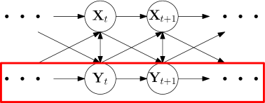
Figure 5: Schematic diagram of a discrete-time Markov process in a composite system (where only Y is observable).

The magnitude relationship between total entropy production and marginal entropy production for both time-reversed and backward entropy production is derived below.

4.1.1 Time-Reversed Entropy Production

The magnitude relationship between time-reversed total entropy production and marginal entropy production is shown below.

Result 4.1 (Inequalities for Total Entropy Production and Marginal Entropy Production (Time-Reversed)).

$$\tilde{\Sigma}_{{\mathrm{XY}}}^{{\mathrm{tot}}}\geq\tilde{\Sigma}_{{\mathrm{Y}}}^{{\mathrm{mar}}}$$ (4.1)

Derivation.

This is obtained by setting

$$i \rightarrow\left({\mathbf{x}_{t},\mathbf{x}_{t+1}}\right)$$ (4.2)

$$a_{i} \rightarrow P_{\mathbf{X}_{t+1},\mathbf{Y}_{t+1},\mathbf{X}_{t},\mathbf{Y}_{t}}(\mathbf{x}_{t+1},\mathbf{y}_{t+1},\mathbf{x}_{t},\mathbf{y}_{t})$$ (4.3)

$$b_{i} \rightarrow\tilde{Q}_{\mathbf{X}_{t+1},\mathbf{Y}_{t+1},\mathbf{X}_{t},\mathbf{Y}_{t}}(\mathbf{x}_{t+1},\mathbf{y}_{t+1},\mathbf{x}_{t},\mathbf{y}_{t})$$ (4.4)

in the log sum inequality. The equal sign applies when using any function $f$ that depends only on $\mathbf{y}_{t}$ and $\mathbf{y}_{t+1}$, so that

$$\dfrac{P_{\mathbf{X}_{t+1},\mathbf{Y}_{t+1},\mathbf{X}_{t},\mathbf{Y}_{t}}(\mathbf{x}_{t+1},\mathbf{y}_{t+1},\mathbf{x}_{t},\mathbf{y}_{t})}{\tilde{Q}_{\mathbf{X}_{t+1},\mathbf{Y}_{t+1},\mathbf{X}_{t},\mathbf{Y}_{t}}(\mathbf{x}_{t+1},\mathbf{y}_{t+1},\mathbf{x}_{t},\mathbf{y}_{t})}=f(\mathbf{y}_{t},\mathbf{y}_{t+1})$$ (4.5)

This means that the ratio of the probability distribution of the forward process to the probability distribution of the time-reversed process does not depend on the dynamics of X. ∎

When calculating the time-reversed entropy based on data gathered from multiple interacting systems that are only partially observable, the inequality of (4.1) signifies that the correct time-reversed total entropy production is a quantity that is bounded from below.

Furthermore, from the above magnitude relationship, it can be seen that the conditional entropy production [28] defined in chapter 2 is defined in terms of the difference between the total entropy production and marginal entropy production, so the time-reversed conditional entropy production is always non-negative.

Result 4.2 (Non-Negativity of Conditional Entropy Production).

For time-reversed conditional entropy production $\Sigma_{{\mathrm{X}}}^{{\mathrm{mar}}}$ and time-reversed marginal entropy production $\tilde{\Sigma}_{{\mathrm{X}}}^{{\mathrm{mar}}}$, the following relation holds:

$$\tilde{\Sigma}_{{\mathrm{X|Y}}}\geq 0.$$ (4.6)

4.1.2 Backward Entropy Production

Using the magnitude relationship of the time-reversed total entropy production and time-reversed marginal entropy production, it is possible to derive a similar relationship for backward entropy production.

Result 4.3 (Magnitude Relationship of Total Entropy Production and Marginal Entropy Production (Backward)).

$$\Sigma_{{\mathrm{XY}}}^{{\mathrm{tot}}}+\mathrm{KL}({P_{\mathbf{X}_{t+1}|\mathbf{Y}_{t+1}}}||{P_{\mathbf{X}_{t}|\mathbf{Y}_{t}}})\geq\Sigma_{{\mathrm{Y}}}^{\mathrm{mar}}$$ (4.7)

Derivation.

From the relationship between time-reversed entropy production and backward entropy production,

$$\tilde{\Sigma}_{{\mathrm{XY}}}^{\mathrm{tot}}-\Sigma_{{\mathrm{XY}}}^{\mathrm{tot}} =\mathbb{E}_{{\mathrm{XY}}}\left[{\log\dfrac{P_{\mathbf{X}_{t+1},\mathbf{Y}_{t+1}|\mathbf{X}_{t},\mathbf{Y}_{t}}(\mathbf{x}_{t},\mathbf{y}_{t}|\mathbf{x}_{t+1},\mathbf{y}_{t+1})P_{\mathbf{X}_{t+1},\mathbf{Y}_{t+1}}(\mathbf{x}_{t+1},\mathbf{y}_{t+1})}{P_{\mathbf{X}_{t+1},\mathbf{Y}_{t+1}|\mathbf{X}_{t},\mathbf{Y}_{t}}(\mathbf{x}_{t},\mathbf{y}_{t}|\mathbf{x}_{t+1},\mathbf{y}_{t+1})P_{\mathbf{X}_{t},\mathbf{Y}_{t}}(\mathbf{x}_{t+1},\mathbf{y}_{t+1})}}\right]$$ (4.8)

$$=\mathrm{KL}({P_{\mathbf{X}_{t+1},\mathbf{Y}_{t+1}}}||{P_{\mathbf{X}_{t},\mathbf{Y}_{t}}})$$ (4.9)

$$\tilde{\Sigma}_{{\mathrm{Y}}}^{\mathrm{mar}}-\Sigma_{{\mathrm{Y}}}^{\mathrm{mar}} =\mathbb{E}_{{\mathrm{XY}}}\left[{\log\dfrac{P_{\mathbf{Y}_{t+1}|\mathbf{Y}_{t}}(\mathbf{y}_{t}|\mathbf{y}_{t+1})P_{\mathbf{Y}_{t+1}}(\mathbf{y}_{t+1})}{P_{\mathbf{Y}_{t+1}|\mathbf{Y}_{t}}(\mathbf{y}_{t}|\mathbf{y}_{t+1})P_{\mathbf{Y}_{t}}(\mathbf{y}_{t+1})}}\right]$$ (4.10)

$$=\mathrm{KL}({P_{\mathbf{Y}_{t+1}}}||{P_{\mathbf{Y}_{t}}})$$ (4.11)

Based on this relationship and the inequality $\tilde{\Sigma}_{{\mathrm{XY}}}^{\mathrm{tot}}\geq\tilde{\Sigma}_{{\mathrm{Y}}}^{\mathrm{mar}}$,

$$\Sigma_{{\mathrm{XY}}}^{\mathrm{tot}}+\mathrm{KL}({P_{\mathbf{X}_{t+1},\mathbf{Y}_{t+1}}}||{P_{\mathbf{X}_{t},\mathbf{Y}_{t}}}) \geq\Sigma_{{\mathrm{Y}}}^{\mathrm{mar}}+\mathrm{KL}({P_{\mathbf{Y}_{t+1}}}||{P_{\mathbf{Y}_{t}}})$$ (4.12)

$$\Sigma_{{\mathrm{XY}}}^{{\mathrm{tot}}}+\mathrm{KL}({P_{\mathbf{X}_{t+1}|\mathbf{Y}_{t+1}}}||{P_{\mathbf{X}_{t}|\mathbf{Y}_{t}}}) \geq\Sigma_{{\mathrm{Y}}}^{\mathrm{mar}}$$ (4.13)

∎

Inequality (4.7) signifies that when multiple interacting systems are only partially observable, calculating the backward entropy production from the data of only the observed systems will not necessarily result in a quantity for the correct backward total entropy production that is bounded from below.

In addition, the magnitude relationship indicates that, unlike time-reversed conditional entropy production, the production of backward entropy is not always non-negative.

4.2 Inequalities for Partial Entropy Production and Marginal Entropy Production

In the composite system XY of section 2.2, we consider the case where only Y is observable, and the case where Y is observed based on observations of X. In these situations, it is thought that the partial entropy production of Y and the partial entropy production of Y are respectively suitable for the production of entropy in Y. They can be compared by considering the magnitude relationship between the partial entropy production of Y and the peripheral entropy production of Y. As in the case of total entropy production and marginal entropy production, if a specific magnitude relationship is established, it can provide guidelines for estimating entropy production from actual data when a part of the system can be observed.

The magnitude relationship between partial entropy production and peripheral entropy production is derived for both time-reversed entropy production and backward entropy production.

4.2.1 Time-Reversed Entropy Production

The magnitude relationship between time-reversed partial entropy production and time-reversed marginal entropy production is shown below.

Result 4.4 (Inequalities for Partial Entropy Production and Marginal Entropy Production (Time-Reversed)).

$$\tilde{\Sigma}_{{\mathrm{Y}}}^{{\mathrm{par}}}\geq\tilde{\Sigma}_{{\mathrm{Y}}}^{{\mathrm{mar}}}$$ (4.14)

Derivation.

This is obtained by setting

$$i \rightarrow\left({\mathbf{x}_{t},\mathbf{x}_{t+1}}\right)$$ (4.15)

$$a_{i} \rightarrow P_{\mathbf{X}_{t+1},\mathbf{Y}_{t+1},\mathbf{X}_{t},\mathbf{Y}_{t}}(\mathbf{x}_{t+1},\mathbf{y}_{t+1},\mathbf{x}_{t},\mathbf{y}_{t})$$ (4.16)

$$b_{i} \rightarrow\tilde{Q}^{{\mathrm{par}}}_{\mathbf{X}_{t+1},\mathbf{Y}_{t+1},\mathbf{X}_{t},\mathbf{Y}_{t}}(\mathbf{x}_{t+1},\mathbf{y}_{t+1},\mathbf{x}_{t},\mathbf{y}_{t})$$ (4.17)

The equal sign applies when using any function $f$ that depends only on $\mathbf{y}_{t},\mathbf{y}_{t+1}$

$$\dfrac{P_{\mathbf{X}_{t+1},\mathbf{Y}_{t+1},\mathbf{X}_{t},\mathbf{Y}_{t}}(\mathbf{x}_{t+1},\mathbf{y}_{t+1},\mathbf{x}_{t},\mathbf{y}_{t})}{\tilde{Q}^{{\mathrm{par}}}_{\mathbf{X}_{t+1},\mathbf{Y}_{t+1},\mathbf{X}_{t},\mathbf{Y}_{t}}(\mathbf{x}_{t+1},\mathbf{y}_{t+1},\mathbf{x}_{t},\mathbf{y}_{t})}=f(\mathbf{y}_{t},\mathbf{y}_{t+1})$$ (4.18)

This means that the ratio of the probability distribution of the forward process to the probability distribution of the partial time-reversed process does not depend on the dynamics of X. ∎

When calculating the time-reversed entropy based on data gathered from multiple interacting systems that are only partially observable, the inequality of (4.14) signifies that the correct time-reversed partial entropy production is a quantity that is bounded from below.

4.2.2 Backward Entropy Production

Using the magnitude relationship of the time-reversed partial entropy production and time-reversed marginal entropy production, it is possible to derive a similar relationship for backward entropy production.

Result 4.5 (Magnitude Relationship of Partial Entropy Production and Marginal Entropy Production (Backward)).

$$\Sigma_{{\mathrm{Y}}}^{{\mathrm{par}}}+\mathrm{KL}({P_{\mathbf{X}_{t+1},\mathbf{X}_{t}|\mathbf{Y}_{t+1}}}||{P_{\mathbf{X}_{t+1},\mathbf{X}_{t}|\mathbf{Y}_{t}}})+\mathbb{E}_{{\mathrm{XY}}}\left[{\log\dfrac{P_{\mathbf{Y}_{t+1}|\mathbf{Y}_{t},\mathbf{X}_{t+1},\mathbf{X}_{t}}(\mathbf{y}_{t}|\mathbf{y}_{t+1},\mathbf{x}_{t},\mathbf{x}_{t+1})}{P_{\mathbf{Y}_{t+1}|\mathbf{Y}_{t},\mathbf{X}_{t+1},\mathbf{X}_{t}}(\mathbf{y}_{t}|\mathbf{y}_{t+1},\mathbf{x}_{t+1},\mathbf{x}_{t})}}\right]\geq\Sigma_{{\mathrm{Y}}}^{\mathrm{mar}}$$ (4.19)

Derivation.

From the relationship between time-reversed entropy production and backward entropy production,

$$\tilde{\Sigma}_{{\mathrm{Y}}}^{\mathrm{par}}-\Sigma_{{\mathrm{Y}}}^{\mathrm{par}} =\mathbb{E}_{{\mathrm{XY}}}\left[{\log\dfrac{P_{\mathbf{Y}_{t+1}|\mathbf{Y}_{t},\mathbf{X}_{t+1},\mathbf{X}_{t}}(\mathbf{y}_{t}|\mathbf{y}_{t+1},\mathbf{x}_{t+1},\mathbf{x}_{t})P_{\mathbf{Y}_{t+1},\mathbf{X}_{t+1},\mathbf{X}_{t}}(\mathbf{y}_{t+1},\mathbf{x}_{t+1},\mathbf{x}_{t})}{P_{\mathbf{Y}_{t+1}|\mathbf{Y}_{t},\mathbf{X}_{t+1},\mathbf{X}_{t}}(\mathbf{y}_{t}|\mathbf{y}_{t+1},\mathbf{x}_{t+1},\mathbf{x}_{t})P_{\mathbf{Y}_{t},\mathbf{X}_{t+1},\mathbf{X}_{t}}(\mathbf{y}_{t+1},\mathbf{x}_{t+1},\mathbf{x}_{t})}}\right]$$ (4.20)

$$+\mathbb{E}_{{\mathrm{XY}}}\left[{\log\dfrac{P_{\mathbf{Y}_{t+1}|\mathbf{Y}_{t},\mathbf{X}_{t+1},\mathbf{X}_{t}}(\mathbf{y}_{t}|\mathbf{y}_{t+1},\mathbf{x}_{t},\mathbf{x}_{t+1})}{P_{\mathbf{Y}_{t+1}|\mathbf{Y}_{t},\mathbf{X}_{t+1},\mathbf{X}_{t}}(\mathbf{y}_{t}|\mathbf{y}_{t+1},\mathbf{x}_{t+1},\mathbf{x}_{t})}}\right]$$ (4.21)

$$=\mathrm{KL}({P_{\mathbf{Y}_{t+1},\mathbf{X}_{t+1},\mathbf{X}_{t}}}||{P_{\mathbf{Y}_{t},\mathbf{X}_{t+1},\mathbf{X}_{t}}})+\mathbb{E}_{{\mathrm{XY}}}\left[{\log\dfrac{P_{\mathbf{Y}_{t+1}|\mathbf{Y}_{t},\mathbf{X}_{t+1},\mathbf{X}_{t}}(\mathbf{y}_{t}|\mathbf{y}_{t+1},\mathbf{x}_{t},\mathbf{x}_{t+1})}{P_{\mathbf{Y}_{t+1}|\mathbf{Y}_{t},\mathbf{X}_{t+1},\mathbf{X}_{t}}(\mathbf{y}_{t}|\mathbf{y}_{t+1},\mathbf{x}_{t+1},\mathbf{x}_{t})}}\right]$$ (4.22)

$$\tilde{\Sigma}_{{\mathrm{Y}}}^{\mathrm{mar}}-\Sigma_{{\mathrm{Y}}}^{\mathrm{mar}} =\mathbb{E}_{{\mathrm{XY}}}\left[{\log\dfrac{P_{\mathbf{Y}_{t+1}|\mathbf{Y}_{t}}(\mathbf{y}_{t}|\mathbf{y}_{t+1})P_{\mathbf{Y}_{t+1}}(\mathbf{y}_{t+1})}{P_{\mathbf{Y}_{t+1}|\mathbf{Y}_{t}}(\mathbf{y}_{t}|\mathbf{y}_{t+1})P_{\mathbf{Y}_{t}}(\mathbf{y}_{t+1})}}\right]$$ (4.23)

$$=\mathrm{KL}({P_{\mathbf{Y}_{t+1}}}||{P_{\mathbf{Y}_{t}}})$$ (4.24)

Based on this relationship and the inequality $\tilde{\Sigma}_{{\mathrm{Y}}}^{\mathrm{par}}\geq\tilde{\Sigma}_{{\mathrm{Y}}}^{\mathrm{mar}}$

$$\Sigma_{{\mathrm{Y}}}^{\mathrm{par}}+\mathrm{KL}({P_{\mathbf{Y}_{t+1},\mathbf{X}_{t+1},\mathbf{X}_{t}}}||{P_{\mathbf{Y}_{t},\mathbf{X}_{t+1},\mathbf{X}_{t}}})+\mathbb{E}_{{\mathrm{XY}}}\left[{\log\dfrac{P_{\mathbf{Y}_{t+1}|\mathbf{Y}_{t},\mathbf{X}_{t+1},\mathbf{X}_{t}}(\mathbf{y}_{t}|\mathbf{y}_{t+1},\mathbf{x}_{t},\mathbf{x}_{t+1})}{P_{\mathbf{Y}_{t+1}|\mathbf{Y}_{t},\mathbf{X}_{t+1},\mathbf{X}_{t}}(\mathbf{y}_{t}|\mathbf{y}_{t+1},\mathbf{x}_{t+1},\mathbf{x}_{t})}}\right] \geq\Sigma_{{\mathrm{Y}}}^{\mathrm{mar}}+\mathrm{KL}({P_{\mathbf{Y}_{t+1}}}||{P_{\mathbf{Y}_{t}}})$$ (4.25)

$$\Sigma_{{\mathrm{Y}}}^{{\mathrm{par}}}+\mathrm{KL}({P_{\mathbf{X}_{t+1},\mathbf{X}_{t}|\mathbf{Y}_{t+1}}}||{P_{\mathbf{X}_{t+1},\mathbf{X}_{t}|\mathbf{Y}_{t}}})+\mathbb{E}_{{\mathrm{XY}}}\left[{\log\dfrac{P_{\mathbf{Y}_{t+1}|\mathbf{Y}_{t},\mathbf{X}_{t+1},\mathbf{X}_{t}}(\mathbf{y}_{t}|\mathbf{y}_{t+1},\mathbf{x}_{t},\mathbf{x}_{t+1})}{P_{\mathbf{Y}_{t+1}|\mathbf{Y}_{t},\mathbf{X}_{t+1},\mathbf{X}_{t}}(\mathbf{y}_{t}|\mathbf{y}_{t+1},\mathbf{x}_{t+1},\mathbf{x}_{t})}}\right] \geq\Sigma_{{\mathrm{Y}}}^{\mathrm{mar}}$$ (4.26)

∎

Inequality (4.19) signifies that when multiple interacting systems are only partially observable, calculating the backward entropy production from the data of only the observed systems will not necessarily result in a quantity for the correct backward partial entropy production that is bounded from below.

5 Example: Gaussian process

In this chapter, we derive the entropy production for Gaussian process. Section 5.1 defines Gaussian process. In sections 5.2, 5.3 and 5.4, we calculate the total entropy production, partial entropy production and marginal entropy production for Gaussian process. In section 5.5, we set appropriate parameters based on the analytical results, and illustrate the numerical results.

Note that the partial entropy production for composite Gaussian process in continuous time as discussed in references [15, 18] among others.

5.1 Definitions

Gaussian process is defined by a stochastic process where probability distribution at any time is Gaussian distribution. An example is the Kalman filter, which is widely used in time-series data analysis [37].

Here, we will first define the distributions of X and Y at times $t$ and $t+1$, and then derive the distribution at each time, the conditional distribution, the difference equation, and the marginal distribution of X.

Joint Distribution at Times $t$ and $t+1$

When the systems X and Y evolve over time from $t$ to $t+1$ while interacting, the joint distribution $\mathbf{X}_{t:t+1},\mathbf{Y}_{t:t+1}$ is given by the following multidimensional Gaussian distribution:

$$P_{\mathbf{X}_{t:t+1},\mathbf{Y}_{t:t+1}}(\mathbf{x}_{t:t+1},\mathbf{y}_{t:t+1})=\mathcal{N}_{\mathbf{x}_{t:t+1},\mathbf{y}_{t:t+1}}(\bm{\mu},\mathbf{K})$$ (5.1)

$$\bm{\mu}={\begin{pmatrix}\bm{\mu}_{\mathbf{X}_{t}}&\bm{\mu}_{\mathbf{Y}_{t}}&\bm{\mu}_{\mathbf{X}_{t+1}}&\bm{\mu}_{\mathbf{Y}_{t+1}}\end{pmatrix}}^{\top}$$ (5.2)

$$\mathbf{K}=\begin{pmatrix}\mathbf{K}_{\mathbf{x}_{t}\mathbf{x}_{t}}&\mathbf{K}_{\mathbf{x}_{t}\mathbf{y}_{t}}&\mathbf{K}_{\mathbf{x}_{t}\mathbf{x}_{t+1}}&\mathbf{K}_{\mathbf{x}_{t}\mathbf{y}_{t+1}}\\ \mathbf{K}_{\mathbf{y}_{t}\mathbf{x}_{t}}&\mathbf{K}_{\mathbf{y}_{t}\mathbf{y}_{t}}&\mathbf{K}_{\mathbf{y}_{t}\mathbf{x}_{t+1}}&\mathbf{K}_{\mathbf{y}_{t}\mathbf{y}_{t+1}}\\ \mathbf{K}_{\mathbf{x}_{t+1}\mathbf{x}_{t}}&\mathbf{K}_{\mathbf{x}_{t+1}\mathbf{y}_{t}}&\mathbf{K}_{\mathbf{x}_{t+1}\mathbf{x}_{t+1}}&\mathbf{K}_{\mathbf{x}_{t+1}\mathbf{y}_{t+1}}\\ \mathbf{K}_{\mathbf{y}_{t+1}\mathbf{x}_{t}}&\mathbf{K}_{\mathbf{y}_{t+1}\mathbf{y}_{t}}&\mathbf{K}_{\mathbf{y}_{t+1}\mathbf{x}_{t+1}}&\mathbf{K}_{\mathbf{y}_{t+1}\mathbf{y}_{t+1}}\end{pmatrix}$$ (5.3)

where

$$\bm{\mu}_{\mathbf{z}_{i}}= \mathbb{E}_{\mathbf{Z}_{i}}\left[{\mathbf{Z}_{i}}\right]$$ (5.4)

$$\mathbf{K}_{\mathbf{z}_{i}\mathbf{z}^{\prime}_{j}}= \text{Cov}\left[{\mathbf{Z}_{i},\mathbf{Z}^{\prime}_{j}}\right]$$ (5.5)

$$(\mathbf{Z},\mathbf{Z}^{\prime}=\mathbf{X},\mathbf{Y},\quad i,j=t,t+1)$$ (5.6)

Since $\mathbf{K}_{\mathbf{z}^{\prime}_{j}\mathbf{z}_{i}}={\mathbf{K}}^{\top}_{\mathbf{z}_{i}\mathbf{z}^{\prime}_{j}}$ by definition, this is equivalent to

$$\mathbf{K}=\begin{pmatrix}\mathbf{K}_{\mathbf{x}_{t}\mathbf{x}_{t}}&\mathbf{K}_{\mathbf{x}_{t}\mathbf{y}_{t}}&\mathbf{K}_{\mathbf{x}_{t}\mathbf{x}_{t+1}}&\mathbf{K}_{\mathbf{x}_{t}\mathbf{y}_{t+1}}\\ {\mathbf{K}}^{\top}_{\mathbf{x}_{t}\mathbf{y}_{t}}&\mathbf{K}_{\mathbf{y}_{t}\mathbf{y}_{t}}&{\mathbf{K}}^{\top}_{\mathbf{x}_{t}\mathbf{y}_{t+1}}&\mathbf{K}_{\mathbf{y}_{t}\mathbf{y}_{t+1}}\\ {\mathbf{K}}^{\top}_{\mathbf{x}_{t}\mathbf{x}_{t+1}}&{\mathbf{K}}^{\top}_{\mathbf{x}_{t}\mathbf{y}_{t+1}}&\mathbf{K}_{\mathbf{x}_{t+1}\mathbf{x}_{t+1}}&\mathbf{K}_{\mathbf{x}_{t+1}\mathbf{y}_{t+1}}\\ \mathbf{K}_{\mathbf{x}_{t}\mathbf{y}_{t+1}}&{\mathbf{K}}^{\top}_{\mathbf{y}_{t}\mathbf{y}_{t+1}}&{\mathbf{K}}^{\top}_{\mathbf{x}_{t+1}\mathbf{y}_{t+1}}&\mathbf{K}_{\mathbf{y}_{t+1}\mathbf{y}_{t+1}}\end{pmatrix}$$ (5.7)

Furthermore, $\mathbf{X}_{t}$, $\mathbf{X}_{t+1}$, $\mathbf{Y}_{t}$ and $\mathbf{Y}_{t+1}$ are all assumed to be $d$-dimensional vectors.

Joint Distribution at Each Time

The joint distribution at each time is given by

$$P_{\mathbf{X}_{t},\mathbf{Y}_{t}}(\mathbf{x}_{t},\mathbf{y}_{t})= \mathcal{N}_{\mathbf{x}_{t},\mathbf{y}_{t}}(\bm{\mu}_{t},\mathbf{K}_{t,t})$$ (5.8)

$$P_{\mathbf{X}_{t+1},\mathbf{Y}_{t+1}}(\mathbf{x}_{t+1},\mathbf{y}_{t+1})= \mathcal{N}_{\mathbf{x}_{t+1},\mathbf{y}_{t+1}}(\bm{\mu}_{t+1},\mathbf{K}_{t+1,t+1})$$ (5.9)

where

$$\bm{\mu}_{i}={\begin{pmatrix}\bm{\mu}_{\mathbf{x}_{i}}&\bm{\mu}_{\mathbf{y}_{i}}\end{pmatrix}}^{\top}$$ (5.10)

$$\mathbf{K}_{i,j}=\begin{pmatrix}\mathbf{K}_{\mathbf{x}_{i}\mathbf{x}_{j}}&\mathbf{K}_{\mathbf{x}_{i}\mathbf{y}_{j}}\\ {\mathbf{K}}^{\top}_{\mathbf{x}_{i}\mathbf{y}_{j}}&\mathbf{K}_{\mathbf{y}_{i}\mathbf{y}_{j}}\end{pmatrix}$$ (5.11)

$$(i,j=t,t+1)$$ (5.12)

Conditional Distribution

The conditional distribution of X and Y at time $t+1$, based on the conditions of X and Y at time $t$ is given by

$$P_{\mathbf{X}_{t+1},\mathbf{Y}_{t+1}|\mathbf{X}_{t},\mathbf{Y}_{t}}(\mathbf{x}_{t+1},\mathbf{y}_{t+1}|\mathbf{x}_{t},\mathbf{y}_{t})=\mathcal{N}_{\mathbf{x}_{t+1},\mathbf{y}_{t+1}|\mathbf{x}_{t},\mathbf{y}_{t}}(\bm{\mu}_{t+1|t},\mathbf{K}_{t+1|t})$$ (5.13)

where

$$\bm{\mu}_{t+1|t}= \bm{\mu}_{t+1}+{\mathbf{K}}^{\top}_{t,t+1}\mathbf{K}_{t,t}^{-1}\left({\mathbf{s}_{t}-\bm{\mu}_{t}}\right)$$ (5.14)

$$\mathbf{K}_{t+1|t}= \mathbf{K}_{t+1,t+1}-{\mathbf{K}}^{\top}_{t,t+1}\mathbf{K}_{t,t}^{-1}\mathbf{K}_{t,t+1}$$ (5.15)

Difference Equation

In the conditional distribution, $\bm{\mu}_{t+1|t}$ can also be expressed as

$$\bm{\mu}_{t+1|t}= \mathbf{A}\mathbf{s}_{t}+\mathbf{b}$$ (5.16)

$$\mathbf{s}_{t}= {\begin{pmatrix}\mathbf{x}_{t}&\mathbf{y}_{t}\end{pmatrix}}^{\top}$$ (5.17)

$$\mathbf{A}:={\mathbf{K}}^{\top}_{t,t+1}\mathbf{K}_{t,t}^{-1},\quad \mathbf{b}:=\bm{\mu}_{t+1}-{\mathbf{K}}^{\top}_{t,t+1}\mathbf{K}_{t,t}^{-1}\bm{\mu}_{t}$$ (5.18)

and thus the difference equation representing the temporal evolution of systems X and Y can be expressed as follows.

$$\mathbf{s}_{t+1}= \mathbf{A}\mathbf{s}_{t}+\mathbf{b}+\bm{\xi}_{t}$$ (5.19)

$$\mathbf{s}_{t+1}= {\begin{pmatrix}\mathbf{x}_{t+1}&\mathbf{y}_{t+1}\end{pmatrix}}^{\top}$$ (5.20)

$$\bm{\xi}_{t}:= {\begin{pmatrix}\bm{\xi}_{\mathbf{X}_{t}}&\bm{\xi}_{\mathbf{Y}_{t}}\end{pmatrix}}^{\top}$$ (5.21)

Here, $\mathbf{A}$ represents the interaction of systems X and Y in temporal evolution, and $\mathbf{b}$ represents a constant shift. Suppose $\mathbf{A}$ and $\mathbf{b}$ are expressed as follows.

$$\mathbf{A}=\begin{pmatrix}\mathbf{A_{xx}}&\mathbf{A_{xy}}\\ \mathbf{A_{yx}}&\mathbf{A_{yy}}\end{pmatrix}=\begin{pmatrix}\mathbf{A_{x}}\\ \mathbf{A_{y}}\end{pmatrix}$$ (5.22)

$$\mathbf{A_{x}}=\begin{pmatrix}\mathbf{A_{xx}}&\mathbf{A_{xy}}\end{pmatrix}\quad\mathbf{A_{y}}=\begin{pmatrix}\mathbf{A_{yx}}&\mathbf{A_{yy}}\end{pmatrix}$$ (5.23)

$$\mathbf{b}={\begin{pmatrix}\mathbf{b_{x}}&\mathbf{b_{y}}\end{pmatrix}}^{\top}$$ (5.24)

Furthermore, $\bm{\xi}_{t}$ represents Gaussian noise with a mean of zero and a covariance matrix of $\mathbf{K}_{t+1|t}$. In the following, it is assumed that the Gaussian noise $\bm{\xi}_{t}$ is uniform and independent of systems X and Y:

$$\mathbf{K}_{t+1|t}=\lambda^{-1}\mathbf{I}_{2d}$$ (5.25)

where $\lambda$ denotes the accuracy of the noise, and $\mathbf{I}_{2d}$ is a $2d$-dimensional unit matrix.

Also, by using $\mathbf{K}_{t+1|t}$, the following relation is established between the covariance matrices of the simultaneous distributions of X and Y at each time $t$ and $t+1$.

$$\mathbf{K}_{t+1,t+1}= {\mathbf{K}}^{\top}_{t,t+1}\mathbf{K}_{t,t}^{-1}\mathbf{K}_{t,t+1}+\mathbf{K}_{t+1|t}$$ (5.26)

$$= {\mathbf{K}}^{\top}_{t,t+1}\mathbf{K}_{t,t}^{-1}\mathbf{K}_{t,t}\mathbf{K}_{t,t}^{-1}\mathbf{K}_{t,t+1}+\mathbf{K}_{t+1|t}$$ (5.27)

$$= {\mathbf{K}}^{\top}_{t,t+1}\mathbf{K}_{t,t}^{-1}\mathbf{K}_{t,t}{({\mathbf{K}}^{\top}_{t,t+1}\mathbf{K}_{t,t}^{-1})}^{\top}+\mathbf{K}_{t+1|t}$$ (5.28)

$$= \mathbf{A}\mathbf{K}_{t,t}{\mathbf{A}}^{\top}+\mathbf{K}_{t+1|t}$$ (5.29)

Marginal Distribution

The marginal distribution of X is given by

$$P_{\mathbf{X}_{t:t+1}}(\mathbf{x}_{t:t+1})= \mathcal{N}_{\mathbf{x}_{t:t+1}}(\bm{\mu}_{\mathbf{x}},\mathbf{K}_{\mathbf{x}\mathbf{x}})$$ (5.30)

where

$$\bm{\mu}_{\mathbf{x}}={\begin{pmatrix}\bm{\mu}_{\mathbf{x}_{t}}&\bm{\mu}_{\mathbf{x}_{t+1}}\end{pmatrix}}^{\top}$$ (5.31)

$$\mathbf{K}_{\mathbf{x}\mathbf{x}}=\begin{pmatrix}\mathbf{K}_{\mathbf{x}_{t}\mathbf{x}_{t}}&\mathbf{K}_{\mathbf{x}_{t}\mathbf{x}_{t+1}}\\ {\mathbf{K}}^{\top}_{\mathbf{x}_{t}\mathbf{x}_{t+1}}&\mathbf{K}_{\mathbf{x}_{t+1}\mathbf{x}_{t+1}}\end{pmatrix}$$ (5.32)

5.2 Total Entropy Production

Time-Reversed Total Entropy Production

In the relationship

$$\tilde{\Sigma}_{{\mathrm{XY}}}^{{\mathrm{tot}}}=\mathrm{KL}({P_{\mathbf{X}_{t:t+1},\mathbf{Y}_{t:t+1}}}||{\tilde{Q}_{\mathbf{X}_{t:t+1},\mathbf{Y}_{t:t+1}}})$$ (5.33)

We assumed the following identities:

$$P_{\mathbf{X}_{t:t+1},\mathbf{Y}_{t:t+1}}(\mathbf{x}_{t:t+1},\mathbf{y}_{t:t+1})= \mathcal{N}_{\mathbf{s}}(\bm{\mu},\mathbf{K})$$ (5.34)

$$= \frac{1}{\sqrt{|2\pi\mathbf{K}|}}\exp\left[{-\frac{1}{2}{(\mathbf{s}-\bm{\mu})}^{\top}\mathbf{K}^{-1}(\mathbf{s}-\bm{\mu})}\right]$$ (5.35)

$$\tilde{Q}_{\mathbf{X}_{t:t+1},\mathbf{Y}_{t:t+1}}(\mathbf{x}_{t:t+1},\mathbf{y}_{t:t+1})= \frac{1}{\sqrt{|2\pi\mathbf{K}|}}\exp\left[{-\frac{1}{2}{(\tilde{\mathbf{s}}-\bm{\mu})}^{\top}\mathbf{K}^{-1}(\tilde{\mathbf{s}}-\bm{\mu})}\right]$$ (5.36)

where

$$\mathbf{s}={\begin{pmatrix}\mathbf{s}_{t}&\mathbf{s}_{t+1}\end{pmatrix}}^{\top},\quad\tilde{\mathbf{s}}={\begin{pmatrix}\mathbf{s}_{t+1}&\mathbf{s}_{t}\end{pmatrix}}^{\top}$$ (5.37)

Consider rewriting the variable of the time-reversed distribution with $\mathbf{s}$. From the inverse matrix[37, 38] of the block matrix, we obtain

$$\mathbf{K}^{-1}= \begin{pmatrix}\mathbf{K}_{t|t+1}^{-1}&-\mathbf{K}_{t,t}^{-1}\mathbf{K}_{t,t+1}\mathbf{K}_{t+1|t}^{-1}\\ -\mathbf{K}_{t+1|t}^{-1}{\mathbf{K}}^{\top}_{t,t+1}\mathbf{K}_{t,t}^{-1}&\mathbf{K}_{t+1|t}^{-1}\end{pmatrix}$$ (5.38)

$$= \begin{pmatrix}\mathbf{K}_{t|t+1}^{-1}&-{\mathbf{A}}^{\top}\mathbf{K}_{t+1|t}^{-1}\\ -\mathbf{K}_{t+1|t}^{-1}\mathbf{A}&\mathbf{K}_{t+1|t}^{-1}\end{pmatrix}$$ (5.39)

where it is assumed that

$$\mathbf{K}_{t|t+1}:=\mathbf{K}_{t,t}-\mathbf{K}_{t,t+1}\mathbf{K}_{t+1,t+1}^{-1}{\mathbf{K}}^{\top}_{t,t+1}$$ (5.40)

Therefore, the secondary term of the exponential part of the time-reversed distribution $\tilde{Q}_{\mathbf{X}_{t:t+1},\mathbf{Y}_{t:t+1}}$ becomes

$${(\tilde{\mathbf{s}}-\bm{\mu})}^{\top}\mathbf{K}^{-1}(\tilde{\mathbf{s}}-\bm{\mu})= {(\mathbf{s}_{t+1}-\bm{\mu}_{t})}^{\top}\mathbf{K}_{t|t+1}^{-1}(\mathbf{s}_{t+1}-\bm{\mu}_{t})+{(\mathbf{s}_{t+1}-\bm{\mu}_{t})}^{\top}\left({-{\mathbf{A}}^{\top}\mathbf{K}_{t+1|t}^{-1}}\right)(\mathbf{s}_{t}-\bm{\mu}_{t+1})$$ (5.41)

$$+{(\mathbf{s}_{t}-\bm{\mu}_{t+1})}^{\top}\left({-\mathbf{K}_{t+1|t}^{-1}\mathbf{A}}\right)(\mathbf{s}_{t+1}-\bm{\mu}_{t})+{(\mathbf{s}_{t}-\bm{\mu}_{t+1})}^{\top}\mathbf{K}_{t+1|t}^{-1}(\mathbf{s}_{t}-\bm{\mu}_{t+1})$$ (5.42)

$$= {(\mathbf{s}-\tilde{\bm{\mu}})}^{\top}\tilde{\mathbf{K}}^{-1}(\mathbf{s}-\tilde{\bm{\mu}})$$ (5.43)

where it is assumed that

$$\tilde{\bm{\mu}}:= {\begin{pmatrix}\bm{\mu}_{t+1}&\bm{\mu}_{t}\end{pmatrix}}^{\top}$$ (5.44)

$$\tilde{\mathbf{K}}^{-1}:= \begin{pmatrix}\mathbf{K}_{t+1|t}^{-1}&-\mathbf{K}_{t+1|t}^{-1}\mathbf{A}\\ -{\mathbf{A}}^{\top}\mathbf{K}_{t+1|t}^{-1}&\mathbf{K}_{t|t+1}^{-1}\end{pmatrix}$$ (5.45)

Also, from the determinant of the block matrix [37, 38],

$$|\mathbf{K}^{-1}| =\left|\mathbf{K}_{t|t+1}^{-1}\right|\left|\mathbf{K}_{t+1|t}^{-1}-\mathbf{K}_{t+1|t}^{-1}\mathbf{A}\mathbf{K}_{t|t+1}{\mathbf{A}}^{\top}\mathbf{K}_{t+1|t}^{-1}\right|$$ (5.46)

$$|\tilde{\mathbf{K}}^{-1}| =\left|\mathbf{K}_{t|t+1}^{-1}\right|\left|\mathbf{K}_{t+1|t}^{-1}-\mathbf{K}_{t+1|t}^{-1}\mathbf{A}\mathbf{K}_{t|t+1}{\mathbf{A}}^{\top}\mathbf{K}_{t+1|t}^{-1}\right|$$ (5.47)

$$=|\mathbf{K}^{-1}|$$ (5.48)

which yields the following expression:

$$\tilde{Q}_{\mathbf{X}_{t:t+1},\mathbf{Y}_{t:t+1}}(\mathbf{x}_{t:t+1},\mathbf{y}_{t:t+1})= \frac{1}{\sqrt{|2\pi\tilde{\mathbf{K}}|}}\exp\left[{-\frac{1}{2}{(\mathbf{s}-\tilde{\bm{\mu}})}^{\top}\tilde{\mathbf{K}}^{-1}(\mathbf{s}-\tilde{\bm{\mu}})}\right]$$ (5.49)

$$= \mathcal{N}_{\mathbf{s}}(\tilde{\bm{\mu}},\tilde{\mathbf{K}})$$ (5.50)

Based on the above, the time-reversed total entropy production from the KLD of the multidimensional Gaussian distribution is as follows:

$$\tilde{\Sigma}_{{\mathrm{XY}}}^{{\mathrm{tot}}}= \frac{1}{2}\left\{{\mathrm{Tr}\left[\tilde{\mathbf{K}}^{-1}\mathbf{K}\right]-4d+{(\tilde{\bm{\mu}}-\bm{\mu})}^{\top}\tilde{\mathbf{K}}^{-1}(\tilde{\bm{\mu}}-\bm{\mu})+\log\frac{|\tilde{\mathbf{K}}|}{|\mathbf{K}|}}\right\}$$ (5.51)

$$= \frac{1}{2}\left\{{\mathrm{Tr}\left[\tilde{\mathbf{K}}^{-1}\mathbf{K}\right]-4d+{(\tilde{\bm{\mu}}-\bm{\mu})}^{\top}\tilde{\mathbf{K}}^{-1}(\tilde{\bm{\mu}}-\bm{\mu})}\right\}$$ (5.52)

Here, since $|\mathbf{K}^{-1}|=|\tilde{\mathbf{K}}^{-1}|$, we used the relationship $|\mathbf{K}|=|\tilde{\mathbf{K}}|$.

In the time-reversed total entropy production (5.52), the first term is

$$\tilde{\mathbf{K}}^{-1}\mathbf{K}= \begin{pmatrix}\mathbf{K}_{t+1|t}^{-1}&-\mathbf{K}_{t+1|t}^{-1}\mathbf{A}\\ -{\mathbf{A}}^{\top}\mathbf{K}_{t+1|t}^{-1}&\mathbf{K}_{t|t+1}^{-1}\end{pmatrix}\begin{pmatrix}\mathbf{K}_{t,t}&\mathbf{K}_{t,t+1}\\ {\mathbf{K}}^{\top}_{t,t+1}&\mathbf{K}_{t+1,t+1}\end{pmatrix}$$ (5.53)

$$= \begin{pmatrix}\mathbf{K}_{t+1|t}^{-1}\mathbf{K}_{t,t}-\mathbf{K}_{t+1|t}^{-1}\mathbf{A}{\mathbf{K}}^{\top}_{t,t+1}&\mathbf{K}_{t+1|t}^{-1}\mathbf{K}_{t,t+1}-\mathbf{K}_{t+1|t}^{-1}\mathbf{A}\mathbf{K}_{t+1,t+1}\\ -{\mathbf{A}}^{\top}\mathbf{K}_{t+1|t}^{-1}\mathbf{K}_{t,t}+\mathbf{K}_{t|t+1}^{-1}{\mathbf{K}}^{\top}_{t,t+1}&-{\mathbf{A}}^{\top}\mathbf{K}_{t+1|t}^{-1}\mathbf{K}_{t,t+1}+\mathbf{K}_{t|t+1}^{-1}\mathbf{K}_{t+1,t+1}\end{pmatrix}$$ (5.54)

and so

$$\mathrm{Tr}\left[\tilde{\mathbf{K}}^{-1}\mathbf{K}\right]= \mathrm{Tr}\left[\mathbf{K}_{t+1|t}^{-1}\mathbf{K}_{t,t}-\mathbf{K}_{t+1|t}^{-1}\mathbf{A}{\mathbf{K}}^{\top}_{t,t+1}-{\mathbf{A}}^{\top}\mathbf{K}_{t+1|t}^{-1}\mathbf{K}_{t,t+1}+\mathbf{K}_{t|t+1}^{-1}\mathbf{K}_{t+1,t+1}\right]$$ (5.55)

$$= \lambda\mathrm{Tr}\left[\mathbf{K}_{t,t}-\mathbf{A}{\mathbf{K}}^{\top}_{t,t+1}-{\mathbf{A}}^{\top}\mathbf{K}_{t,t+1}\right]+\mathrm{Tr}\left[\mathbf{K}_{t|t+1}^{-1}\mathbf{K}_{t+1,t+1}\right]$$ (5.56)

According to the Woodbury identity[37, 38], the last term in the above formula can be expanded as shown below.

$$\mathrm{Tr}\left[\mathbf{K}_{t|t+1}^{-1}\mathbf{K}_{t+1,t+1}\right]= \mathrm{Tr}\left[\left({\mathbf{K}_{t,t}^{-1}+{\mathbf{A}}^{\top}\mathbf{K}_{t+1|t}^{-1}\mathbf{A}}\right)\mathbf{K}_{t+1,t+1}\right]$$ (5.57)

$$= \mathrm{Tr}\left[\mathbf{K}_{t,t}^{-1}\mathbf{K}_{t+1,t+1}\right]+\lambda\mathrm{Tr}\left[{\mathbf{A}}^{\top}\mathbf{A}\mathbf{K}_{t+1,t+1}\right]$$ (5.58)

Therefore,

$$\mathrm{Tr}\left[\tilde{\mathbf{K}}^{-1}\mathbf{K}\right]= \lambda\mathrm{Tr}\left[\mathbf{K}_{t,t}-\mathbf{A}{\mathbf{K}}^{\top}_{t,t+1}-{\mathbf{A}}^{\top}\mathbf{K}_{t,t+1}+{\mathbf{A}}^{\top}\mathbf{A}\mathbf{K}_{t+1,t+1}\right]+\mathrm{Tr}\left[\mathbf{K}_{t,t}^{-1}\mathbf{K}_{t+1,t+1}\right]$$ (5.59)

$$= \lambda\mathrm{Tr}\left[\mathbf{K}_{t,t}-\mathbf{A}^{2}\mathbf{K}_{t,t}-{\mathbf{A}}^{\top}\mathbf{K}_{t,t}{\mathbf{A}}^{\top}+{\mathbf{A}}^{\top}\mathbf{A}\left({\mathbf{A}\mathbf{K}_{t,t}{\mathbf{A}}^{\top}+\mathbf{K}_{t+1|t}}\right)\right]+\mathrm{Tr}\left[\mathbf{K}_{t,t}^{-1}\mathbf{K}_{t+1,t+1}\right]$$ (5.60)

$$= \lambda\mathrm{Tr}\left[\mathbf{K}_{t,t}-\mathbf{A}^{2}\mathbf{K}_{t,t}-({\mathbf{A}}^{\top})^{2}\mathbf{K}_{t,t}+{\mathbf{A}}^{\top}\mathbf{A}\left({\mathbf{A}\mathbf{K}_{t,t}{\mathbf{A}}^{\top}+\mathbf{K}_{t+1|t}}\right)\right]+\mathrm{Tr}\left[\mathbf{K}_{t,t}^{-1}\mathbf{K}_{t+1,t+1}\right]$$ (5.61)

$$= \lambda\mathrm{Tr}\left[\mathbf{K}_{t,t}-\mathbf{A}^{2}\mathbf{K}_{t,t}-({\mathbf{A}}^{\top})^{2}\mathbf{K}_{t,t}+({\mathbf{A}}^{\top})^{2}\mathbf{A}^{2}\mathbf{K}_{t,t}+{\mathbf{A}}^{\top}\mathbf{A}\mathbf{K}_{t+1|t}\right]+\mathrm{Tr}\left[\mathbf{K}_{t,t}^{-1}\mathbf{K}_{t+1,t+1}\right]$$ (5.62)

$$= \lambda\mathrm{Tr}\left[\left({\mathbf{I}_{2d}-({\mathbf{A}}^{\top})^{2}}\right)\left({\mathbf{I}_{2d}-\mathbf{A}^{2}}\right)\mathbf{K}_{t,t}\right]+\lambda\mathrm{Tr}\left[{\mathbf{A}}^{\top}\mathbf{A}\mathbf{K}_{t+1|t}\right]+\mathrm{Tr}\left[\mathbf{K}_{t,t}^{-1}\mathbf{K}_{t+1,t+1}\right]$$ (5.63)

$$= \lambda\mathrm{Tr}\left[\left({\mathbf{I}_{2d}-{\mathbf{A}}^{\top}}\right)\left({\mathbf{I}_{2d}+{\mathbf{A}}^{\top}}\right)\left({\mathbf{I}_{2d}-\mathbf{A}}\right)\left({\mathbf{I}_{2d}+\mathbf{A}}\right)\mathbf{K}_{t,t}\right]+\mathrm{Tr}\left[{\mathbf{A}}^{\top}\mathbf{A}\right]+\mathrm{Tr}\left[\mathbf{K}_{t,t}^{-1}\mathbf{K}_{t+1,t+1}\right]$$ (5.64)

The third term can be expanded as follows:

$${(\tilde{\bm{\mu}}-\bm{\mu})}^{\top}\tilde{\mathbf{K}}^{-1}(\tilde{\bm{\mu}}-\bm{\mu})$$ (5.65)

$$= {(\bm{\mu}_{t+1}-\bm{\mu}_{t})}^{\top}\mathbf{K}_{t+1|t}^{-1}(\bm{\mu}_{t+1}-\bm{\mu}_{t})+{(\bm{\mu}_{t+1}-\bm{\mu}_{t})}^{\top}(-\mathbf{K}_{t+1|t}^{-1}\mathbf{A})(\bm{\mu}_{t}-\bm{\mu}_{t+1})$$ (5.66)

$$+{(\bm{\mu}_{t}-\bm{\mu}_{t+1})}^{\top}(-{\mathbf{A}}^{\top}\mathbf{K}_{t+1|t}^{-1})(\bm{\mu}_{t+1}-\bm{\mu}_{t})+{(\bm{\mu}_{t}-\bm{\mu}_{t+1})}^{\top}\mathbf{K}_{t|t+1}^{-1}(\bm{\mu}_{t}-\bm{\mu}_{t+1})$$ (5.67)

$$= {\bm{\mu}}^{\top}_{t+1}\left({\mathbf{K}_{t+1|t}^{-1}+\mathbf{K}_{t+1|t}^{-1}\mathbf{A}+{\mathbf{A}}^{\top}\mathbf{K}_{t+1|t}^{-1}+\mathbf{K}_{t|t+1}^{-1}}\right)\bm{\mu}_{t+1}$$ (5.68)

$$-{\bm{\mu}}^{\top}_{t+1}\left({\mathbf{K}_{t+1|t}^{-1}+\mathbf{K}_{t+1|t}^{-1}\mathbf{A}+{\mathbf{A}}^{\top}\mathbf{K}_{t+1|t}^{-1}+\mathbf{K}_{t|t+1}^{-1}}\right)\bm{\mu}_{t}$$ (5.69)

$$-{\bm{\mu}}^{\top}_{t}\left({\mathbf{K}_{t+1|t}^{-1}+\mathbf{K}_{t+1|t}^{-1}\mathbf{A}+{\mathbf{A}}^{\top}\mathbf{K}_{t+1|t}^{-1}+\mathbf{K}_{t|t+1}^{-1}}\right)\bm{\mu}_{t+1}$$ (5.70)

$$+{\bm{\mu}}^{\top}_{t}\left({\mathbf{K}_{t+1|t}^{-1}+\mathbf{K}_{t+1|t}^{-1}\mathbf{A}+{\mathbf{A}}^{\top}\mathbf{K}_{t+1|t}^{-1}+\mathbf{K}_{t|t+1}^{-1}}\right)\bm{\mu}_{t}$$ (5.71)

$$= {(\bm{\mu}_{t+1}-\bm{\mu}_{t})}^{\top}\mathbf{W}(\bm{\mu}_{t+1}-\bm{\mu}_{t})$$ (5.72)

$$\mathbf{W}:=\mathbf{K}_{t+1|t}^{-1}+\mathbf{K}_{t+1|t}^{-1}\mathbf{A}+{\mathbf{A}}^{\top}\mathbf{K}_{t+1|t}^{-1}+\mathbf{K}_{t|t+1}^{-1}$$ (5.73)

Here, according to the Woodbury identity,

$$\mathbf{K}_{t|t+1}^{-1}= \left({\mathbf{K}_{t,t}-\mathbf{K}_{t,t+1}\mathbf{K}_{t+1,t+1}{\mathbf{K}}^{\top}_{t,t+1}}\right)^{-1}$$ (5.74)

$$= \mathbf{K}_{t,t}^{-1}-\mathbf{K}_{t,t}^{-1}\mathbf{K}_{t,t+1}\left({-\mathbf{K}_{t+1,t+1}+{\mathbf{K}}^{\top}_{t,t+1}\mathbf{K}_{t,t}^{-1}\mathbf{K}_{t,t+1}}\right)^{-1}{\mathbf{K}}^{\top}_{t,t+1}\mathbf{K}_{t,t}^{-1}$$ (5.75)

$$= \mathbf{K}_{t,t}^{-1}-{\mathbf{A}}^{\top}\left({-\mathbf{K}_{t+1,t+1}+\mathbf{A}\mathbf{K}_{t,t+1}}\right)^{-1}\mathbf{A}$$ (5.76)

$$= \mathbf{K}_{t,t}^{-1}-{\mathbf{A}}^{\top}\left({-\mathbf{K}_{t+1,t+1}+\mathbf{A}\mathbf{K}_{t,t}{\mathbf{A}}^{\top}}\right)^{-1}\mathbf{A}$$ (5.77)

$$= \mathbf{K}_{t,t}^{-1}+{\mathbf{A}}^{\top}\mathbf{K}_{t+1|t}^{-1}\mathbf{A}$$ (5.78)

And so,

$$\mathbf{W}= \mathbf{K}_{t+1|t}^{-1}+\mathbf{K}_{t+1|t}^{-1}\mathbf{A}+{\mathbf{A}}^{\top}\mathbf{K}_{t+1|t}^{-1}+\mathbf{K}_{t,t}^{-1}+{\mathbf{A}}^{\top}\mathbf{K}_{t+1|t}^{-1}\mathbf{A}$$ (5.79)

$$= \lambda\left({\mathbf{I}_{2d}+\mathbf{A}}\right)\left({\mathbf{I}_{2d}+{\mathbf{A}}^{\top}}\right)+\mathbf{K}_{t,t}^{-1}$$ (5.80)

Therefore,

$${(\bm{\mu}_{t+1}-\bm{\mu}_{t})}^{\top}\mathbf{W}(\bm{\mu}_{t+1}-\bm{\mu}_{t})$$ (5.81)

$$= \lambda{(\bm{\mu}_{t+1}-\bm{\mu}_{t})}^{\top}\left({\mathbf{I}_{2d}+\mathbf{A}}\right)\left({\mathbf{I}_{2d}+{\mathbf{A}}^{\top}}\right)(\bm{\mu}_{t+1}-\bm{\mu}_{t})+{(\bm{\mu}_{t+1}-\bm{\mu}_{t})}^{\top}\mathbf{K}_{t,t}^{-1}(\bm{\mu}_{t+1}-\bm{\mu}_{t})$$ (5.82)

$$= \lambda{\bm{\mu}}^{\top}_{t}\left({{\mathbf{A}}^{\top}-\mathbf{I}_{2d}}\right)\left({\mathbf{A}+\mathbf{I}_{2d}}\right)\left({{\mathbf{A}}^{\top}+\mathbf{I}_{2d}}\right)\left({\mathbf{A}-\mathbf{I}_{2d}}\right)\bm{\mu}_{t}+{(\bm{\mu}_{t+1}-\bm{\mu}_{t})}^{\top}\mathbf{K}_{t,t}^{-1}(\bm{\mu}_{t+1}-\bm{\mu}_{t})$$ (5.83)

$$= \lambda|\left({{\mathbf{A}}^{\top}\mathbf{A}-\mathbf{I}_{2d}-{\mathbf{A}}^{\top}+\mathbf{A}}\right)\bm{\mu}_{t}|^{2}+{(\bm{\mu}_{t+1}-\bm{\mu}_{t})}^{\top}\mathbf{K}_{t,t}^{-1}(\bm{\mu}_{t+1}-\bm{\mu}_{t})$$ (5.84)

From the above, the time-reversed entropy production can also be expressed as follows:

$$\tilde{\Sigma}_{{\mathrm{XY}}}^{{\mathrm{tot}}}= \frac{1}{2}\bigg{\{}\lambda\mathrm{Tr}\left[\left({\mathbf{I}_{2d}-{\mathbf{A}}^{\top}}\right)\left({\mathbf{I}_{2d}+{\mathbf{A}}^{\top}}\right)\left({\mathbf{I}_{2d}-\mathbf{A}}\right)\left({\mathbf{I}_{2d}+\mathbf{A}}\right)\mathbf{K}_{t,t}\right]+\mathrm{Tr}\left[{\mathbf{A}}^{\top}\mathbf{A}+\mathbf{K}_{t,t}^{-1}\mathbf{K}_{t+1,t+1}\right]-4d$$

$$+\lambda|\left({{\mathbf{A}}^{\top}\mathbf{A}-\mathbf{I}_{2d}-{\mathbf{A}}^{\top}+\mathbf{A}}\right)\bm{\mu}_{t}|^{2}+{(\bm{\mu}_{t+1}-\bm{\mu}_{t})}^{\top}\mathbf{K}_{t,t}^{-1}(\bm{\mu}_{t+1}-\bm{\mu}_{t})\bigg{\}}$$ (5.85)

Backward total entropy production

The backward total entropy production is related to the time-reversed total entropy production by the formula

$$\Sigma_{{\mathrm{XY}}}^{{\mathrm{tot}}}= \tilde{\Sigma}_{{\mathrm{XY}}}^{{\mathrm{tot}}}-\mathrm{KL}({P_{\mathbf{X}_{t+1},\mathbf{Y}_{t+1}}}||{P_{\mathbf{X}_{t},\mathbf{Y}_{t}}})$$ (5.86)

where the second term is equal to

$$\mathrm{KL}({P_{\mathbf{X}_{t+1},\mathbf{Y}_{t+1}}}||{P_{\mathbf{X}_{t},\mathbf{Y}_{t}}})= \frac{1}{2}\left\{{\mathrm{Tr}\left[\mathbf{K}_{t,t}^{-1}\mathbf{K}_{t+1,t+1}\right]-2d+{(\bm{\mu}_{t}-\bm{\mu}_{t+1})}^{\top}\mathbf{K}_{t,t}^{-1}(\bm{\mu}_{t}-\bm{\mu}_{t+1})+\log\frac{|\mathbf{K}_{t,t}|}{|\mathbf{K}_{t+1,t+1}|}}\right\}$$ (5.87)

Therefore, the backward total entropy production is as follows:

$$\Sigma_{{\mathrm{XY}}}^{{\mathrm{tot}}}= \frac{1}{2}\left\{{\mathrm{Tr}\left[\tilde{\mathbf{K}}^{-1}\mathbf{K}\right]-4d+{(\tilde{\bm{\mu}}-\bm{\mu})}^{\top}\tilde{\mathbf{K}}^{-1}(\tilde{\bm{\mu}}-\bm{\mu})}\right\}$$ (5.88)

$$-\frac{1}{2}\left\{{\mathrm{Tr}\left[\mathbf{K}_{t,t}^{-1}\mathbf{K}_{t+1,t+1}\right]-2d+{(\bm{\mu}_{t}-\bm{\mu}_{t+1})}^{\top}\mathbf{K}_{t,t}^{-1}(\bm{\mu}_{t}-\bm{\mu}_{t+1})+\log\frac{|\mathbf{K}_{t,t}|}{|\mathbf{K}_{t+1,t+1}|}}\right\}$$ (5.89)

$$= \frac{1}{2}\bigg{\{}\mathrm{Tr}\left[\tilde{\mathbf{K}}^{-1}\mathbf{K}\right]-\mathrm{Tr}\left[\mathbf{K}_{t,t}^{-1}\mathbf{K}_{t+1,t+1}\right]-2d$$ (5.90)

$$+{(\tilde{\bm{\mu}}-\bm{\mu})}^{\top}\tilde{\mathbf{K}}^{-1}(\tilde{\bm{\mu}}-\bm{\mu})-{(\bm{\mu}_{t}-\bm{\mu}_{t+1})}^{\top}\mathbf{K}_{t,t}^{-1}(\bm{\mu}_{t}-\bm{\mu}_{t+1})+\log\frac{|\mathbf{K}_{t+1,t+1}|}{|\mathbf{K}_{t,t}|}\bigg{\}}$$ (5.91)

$$= \frac{1}{2}\bigg{\{}\lambda\mathrm{Tr}\left[\left({\mathbf{I}_{2d}-{\mathbf{A}}^{\top}}\right)\left({\mathbf{I}_{2d}+{\mathbf{A}}^{\top}}\right)\left({\mathbf{I}_{2d}-\mathbf{A}}\right)\left({\mathbf{I}_{2d}+\mathbf{A}}\right)\mathbf{K}_{t,t}\right]+\mathrm{Tr}\left[{\mathbf{A}}^{\top}\mathbf{A}\right]-2d$$

$$+\lambda|\left({{\mathbf{A}}^{\top}\mathbf{A}-\mathbf{I}_{2d}-{\mathbf{A}}^{\top}+\mathbf{A}}\right)\bm{\mu}_{t}|^{2}+\log\frac{|\mathbf{K}_{t+1,t+1}|}{|\mathbf{K}_{t,t}|}\bigg{\}}$$ (5.92)

5.3 Partial Entropy Production

Time-Reversed Partial Entropy Production

In the relationship

$$\tilde{\Sigma}_{{\mathrm{X}}}^{\mathrm{par}}=\mathrm{KL}({P_{\mathbf{X}_{t:t+1},\mathbf{Y}_{t:t+1}}}||{\tilde{Q}_{\mathbf{X}_{t:t+1},\mathbf{Y}_{t:t+1}}^{{\mathrm{par}}}})$$ (5.93)

the following relations hold

$$P_{\mathbf{X}_{t:t+1},\mathbf{Y}_{t:t+1}}(\mathbf{x}_{t:t+1},\mathbf{y}_{t:t+1})= \mathcal{N}_{\mathbf{s}}(\bm{\mu},\mathbf{K})$$ (5.94)

$$= \frac{1}{\sqrt{|2\pi\mathbf{K}|}}\exp\left[{-\frac{1}{2}{(\mathbf{s}-\bm{\mu})}^{\top}\mathbf{K}^{-1}(\mathbf{s}-\bm{\mu})}\right]$$ (5.95)

$$\tilde{Q}_{\mathbf{X}_{t:t+1},\mathbf{Y}_{t:t+1}}^{{\mathrm{par}}}(\mathbf{x}_{t:t+1},\mathbf{y}_{t:t+1})= \frac{1}{\sqrt{|2\pi\mathbf{K}|}}\exp\left[{-\frac{1}{2}{(\tilde{\mathbf{s}}^{{\mathrm{par}}}-\bm{\mu})}^{\top}\mathbf{K}^{-1}(\tilde{\mathbf{s}}^{{\mathrm{par}}}-\bm{\mu})}\right]$$ (5.96)

where it is assumed that

$$\tilde{\mathbf{s}}^{{\mathrm{par}}}={\begin{pmatrix}\mathbf{x}_{t+1}&\mathbf{y}_{t}&\mathbf{x}_{t}&\mathbf{y}_{t+1}\end{pmatrix}}^{\top}$$ (5.97)

Consider rewriting the variables of the partial time-reversed distribution with $\mathbf{s}$. If the secondary term of the exponential part of the partial time-reversed distribution $\tilde{Q}_{\mathbf{X}_{t:t+1},\mathbf{Y}_{t:t+1}}^{{\mathrm{par}}}$ is assumed to be

$$\mathbf{K}^{-1}= \begin{pmatrix}\mathbf{P}^{1}&\mathbf{P}^{2}\\ \mathbf{P}^{3}&\mathbf{P}^{4}\end{pmatrix}$$ (5.98)

$$\mathbf{P}^{1}=\mathbf{K}_{t|t+1}^{-1},\quad\mathbf{P}^{2}=-{\mathbf{A}}^{\top}\mathbf{K}_{t+1|t}^{-1}, \quad\mathbf{P}^{3}=-\mathbf{K}_{t+1|t}^{-1}\mathbf{A},\quad\mathbf{P}^{4}=\mathbf{K}_{t+1|t}^{-1}$$ (5.99)

$$\mathbf{P}^{i}= \begin{pmatrix}\mathbf{P}^{i}_{\mathbf{xx}}&\mathbf{P}^{i}_{\mathbf{xy}}\\ \mathbf{P}^{i}_{\mathbf{yx}}&\mathbf{P}^{i}_{\mathbf{yy}}\end{pmatrix}\quad\left({i=1,2,3,4}\right)$$ (5.100)

then it can be expanded as follows:

$${(\tilde{\mathbf{s}}^{{\mathrm{par}}}-\bm{\mu})}^{\top}\mathbf{K}^{-1}(\tilde{\mathbf{s}}^{{\mathrm{par}}}-\bm{\mu})$$ (5.101)

$$={(\mathbf{s}_{t+1}-\bm{\mu}_{t})}^{\top}\mathbf{P}^{1}(\mathbf{s}_{t+1}-\bm{\mu}_{t})+{(\mathbf{s}_{t+1}-\bm{\mu}_{t})}^{\top}\mathbf{P}^{2}(\mathbf{s}_{t}-\bm{\mu}_{t+1})$$ (5.102)

$$+{(\mathbf{s}_{t}-\bm{\mu}_{t+1})}^{\top}\mathbf{P}^{3}(\mathbf{s}_{t+1}-\bm{\mu}_{t})+{(\mathbf{s}_{t}-\bm{\mu}_{t+1})}^{\top}\mathbf{P}^{4}(\mathbf{s}_{t}-\bm{\mu}_{t+1})$$ (5.103)

$$={(\mathbf{x}_{t+1}-\bm{\mu}_{\mathbf{x}_{t}})}^{\top}\mathbf{P}^{1}_{\mathbf{xx}}(\mathbf{x}_{t+1}-\bm{\mu}_{\mathbf{x}_{t}})+{(\mathbf{x}_{t+1}-\bm{\mu}_{\mathbf{x}_{t}})}^{\top}\mathbf{P}^{1}_{\mathbf{xy}}(\mathbf{y}_{t}-\bm{\mu}_{\mathbf{y}_{t}})$$ (5.104)

$$+{(\mathbf{y}_{t}-\bm{\mu}_{\mathbf{y}_{t}})}^{\top}\mathbf{P}^{1}_{\mathbf{yx}}(\mathbf{x}_{t+1}-\bm{\mu}_{\mathbf{x}_{t}})+{(\mathbf{y}_{t}-\bm{\mu}_{\mathbf{y}_{t}})}^{\top}\mathbf{P}^{1}_{\mathbf{yy}}(\mathbf{y}_{t}-\bm{\mu}_{\mathbf{y}_{t}})$$ (5.105)

$$+{(\mathbf{x}_{t+1}-\bm{\mu}_{\mathbf{x}_{t}})}^{\top}\mathbf{P}^{2}_{\mathbf{xx}}(\mathbf{x}_{t}-\bm{\mu}_{\mathbf{x}_{t+1}})+{(\mathbf{x}_{t+1}-\bm{\mu}_{\mathbf{x}_{t}})}^{\top}\mathbf{P}^{2}_{\mathbf{xy}}(\mathbf{y}_{t+1}-\bm{\mu}_{\mathbf{y}_{t+1}})$$ (5.106)

$$+{(\mathbf{y}_{t}-\bm{\mu}_{\mathbf{y}_{t}})}^{\top}\mathbf{P}^{2}_{\mathbf{yx}}(\mathbf{x}_{t}-\bm{\mu}_{\mathbf{x}_{t+1}})+{(\mathbf{y}_{t}-\bm{\mu}_{\mathbf{y}_{t}})}^{\top}\mathbf{P}^{2}_{\mathbf{yy}}(\mathbf{y}_{t+1}-\bm{\mu}_{\mathbf{y}_{t+1}})$$ (5.107)

$$+{(\mathbf{x}_{t}-\bm{\mu}_{\mathbf{x}_{t+1}})}^{\top}\mathbf{P}^{3}_{\mathbf{xx}}(\mathbf{x}_{t+1}-\bm{\mu}_{\mathbf{x}_{t}})+{(\mathbf{x}_{t}-\bm{\mu}_{\mathbf{x}_{t+1}})}^{\top}\mathbf{P}^{3}_{\mathbf{xy}}(\mathbf{y}_{t}-\bm{\mu}_{\mathbf{y}_{t}})$$ (5.108)

$$+{(\mathbf{y}_{t+1}-\bm{\mu}_{\mathbf{y}_{t+1}})}^{\top}\mathbf{P}^{3}_{\mathbf{yx}}(\mathbf{x}_{t+1}-\bm{\mu}_{\mathbf{x}_{t}})+{(\mathbf{y}_{t+1}-\bm{\mu}_{\mathbf{y}_{t+1}})}^{\top}\mathbf{P}^{3}_{\mathbf{yy}}(\mathbf{y}_{t}-\bm{\mu}_{\mathbf{y}_{t}})$$ (5.109)

$$+{(\mathbf{x}_{t}-\bm{\mu}_{\mathbf{x}_{t+1}})}^{\top}\mathbf{P}^{4}_{\mathbf{xx}}(\mathbf{x}_{t}-\bm{\mu}_{\mathbf{x}_{t+1}})+{(\mathbf{x}_{t}-\bm{\mu}_{\mathbf{x}_{t+1}})}^{\top}\mathbf{P}^{4}_{\mathbf{xy}}(\mathbf{y}_{t+1}-\bm{\mu}_{\mathbf{y}_{t+1}})$$ (5.110)

$$+{(\mathbf{y}_{t+1}-\bm{\mu}_{\mathbf{y}_{t+1}})}^{\top}\mathbf{P}^{4}_{\mathbf{yx}}(\mathbf{x}_{t}-\bm{\mu}_{\mathbf{x}_{t+1}})+{(\mathbf{y}_{t+1}-\bm{\mu}_{\mathbf{y}_{t+1}})}^{\top}\mathbf{P}^{4}_{\mathbf{yy}}(\mathbf{y}_{t+1}-\bm{\mu}_{\mathbf{y}_{t+1}})$$ (5.111)

$$={(\mathbf{s}_{t}-\bm{\mu}_{t+1})}^{\top}\mathbf{P^{\prime}}^{1}(\mathbf{s}_{t}-\bm{\mu}_{t+1})+{(\mathbf{s}_{t}-\bm{\mu}_{t+1})}^{\top}\mathbf{P^{\prime}}^{2}(\mathbf{s}_{t+1}-\bm{\mu}_{t})$$ (5.112)

$$+{(\mathbf{s}_{t+1}-\bm{\mu}_{t})}^{\top}\mathbf{P^{\prime}}^{3}(\mathbf{s}_{t}-\bm{\mu}_{t+1})+{(\mathbf{s}_{t+1}-\bm{\mu}_{t})}^{\top}\mathbf{P^{\prime}}^{4}(\mathbf{s}_{t+1}-\bm{\mu}_{t})$$ (5.113)

$$={(\mathbf{s}-\tilde{\bm{\mu}}^{{\mathrm{par}}})}^{\top}\left({\tilde{\mathbf{K}}^{{\mathrm{par}}}}\right)^{-1}(\mathbf{s}-\tilde{\bm{\mu}}^{{\mathrm{par}}})$$ (5.114)

Here, it is assumed that

$$\tilde{\bm{\mu}}^{{\mathrm{par}}}:= {\begin{pmatrix}\bm{\mu}_{\mathbf{x}_{t+1}}&\bm{\mu}_{\mathbf{y}_{t}}&\bm{\mu}_{\mathbf{x}_{t}}&\bm{\mu}_{\mathbf{y}_{t+1}}\end{pmatrix}}^{\top}$$ (5.115)

$$\left({\tilde{\mathbf{K}}^{{\mathrm{par}}}}\right)^{-1}:= \begin{pmatrix}\mathbf{P^{\prime}}^{1}&\mathbf{P^{\prime}}^{2}\\ \mathbf{P^{\prime}}^{3}&\mathbf{P^{\prime}}^{4}\end{pmatrix}$$ (5.116)

$$\mathbf{P^{\prime}}^{1}=\begin{pmatrix}\mathbf{P}^{4}_{\mathbf{xx}}&\mathbf{P}^{3}_{\mathbf{xy}}\\ \mathbf{P}^{2}_{\mathbf{yx}}&\mathbf{P}^{1}_{\mathbf{yy}}\end{pmatrix}\mathbf{P^{\prime}}^{2}=\begin{pmatrix}\mathbf{P}^{3}_{\mathbf{xx}}&\mathbf{P}^{4}_{\mathbf{xy}}\\ \mathbf{P}^{1}_{\mathbf{yx}}&\mathbf{P}^{2}_{\mathbf{yy}}\end{pmatrix} \mathbf{P^{\prime}}^{3}=\begin{pmatrix}\mathbf{P}^{2}_{\mathbf{xx}}&\mathbf{P}^{1}_{\mathbf{xy}}\\ \mathbf{P}^{4}_{\mathbf{yx}}&\mathbf{P}^{3}_{\mathbf{yy}}\end{pmatrix}\mathbf{P^{\prime}}^{4}=\begin{pmatrix}\mathbf{P}^{1}_{\mathbf{xx}}&\mathbf{P}^{2}_{\mathbf{xy}}\\ \mathbf{P}^{3}_{\mathbf{yx}}&\mathbf{P}^{4}_{\mathbf{yy}}\end{pmatrix}$$ (5.117)

It can therefore be expressed in the following way

$$\tilde{Q}_{\mathbf{X}_{t:t+1},\mathbf{Y}_{t:t+1}}^{{\mathrm{par}}}(\mathbf{x}_{t:t+1},\mathbf{y}_{t:t+1})= \frac{1}{\sqrt{|2\pi\tilde{\mathbf{K}}^{{\mathrm{par}}}|}}\exp\left[{-\frac{1}{2}{(\mathbf{s}-\tilde{\bm{\mu}}^{{\mathrm{par}}})}^{\top}\left({\tilde{\mathbf{K}}^{{\mathrm{par}}}}\right)^{-1}(\mathbf{s}-\tilde{\bm{\mu}}^{{\mathrm{par}}})}\right]$$ (5.118)

$$= \mathcal{N}_{\mathbf{s}}(\tilde{\bm{\mu}}^{{\mathrm{par}}},\tilde{\mathbf{K}}^{{\mathrm{par}}})$$ (5.119)

by using the identity $|\tilde{\mathbf{K}}^{{\mathrm{par}}}|=|\mathbf{K}|$.

From the above, the time-reversed partial entropy production can be expressed in terms of a multidimensional Gaussian distribution KLD as follows.

$$\tilde{\Sigma}_{{\mathrm{X}}}^{{\mathrm{par}}}= \frac{1}{2}\left\{{\mathrm{Tr}\left[\left({\tilde{\mathbf{K}}^{{\mathrm{par}}}}\right)^{-1}\mathbf{K}\right]-4d+{(\tilde{\bm{\mu}}^{{\mathrm{par}}}-\bm{\mu})}^{\top}\left({\tilde{\mathbf{K}}^{{\mathrm{par}}}}\right)^{-1}(\tilde{\bm{\mu}}^{{\mathrm{par}}}-\bm{\mu})}\right\}$$ (5.120)

Backward Partial Entropy Production

The backward partial entropy production is related to the time-reversed total entropy production by the following formula based on (3.41).

$$\Sigma_{{\mathrm{X}}}^{\mathrm{par}}-\tilde{\Sigma}_{{\mathrm{XY}}}^{\mathrm{tot}} =\mathbb{E}_{\mathbf{X}_{t:t+1},\mathbf{Y}_{t:t+1}}\left[{\log\frac{P_{\mathbf{X}_{t+1}|\mathbf{Y}_{t+1},\mathbf{X}_{t},\mathbf{Y}_{t}}(\mathbf{x}_{t}|\mathbf{y}_{t},\mathbf{x}_{t+1},\mathbf{y}_{t+1})P_{\mathbf{X}_{t},\mathbf{Y}_{t+1},\mathbf{Y}_{t}}(\mathbf{x}_{t+1},\mathbf{y}_{t+1},\mathbf{y}_{t})}{P_{\mathbf{X}_{t+1}|\mathbf{Y}_{t+1},\mathbf{X}_{t},\mathbf{Y}_{t}}(\mathbf{x}_{t}|\mathbf{y}_{t},\mathbf{x}_{t+1},\mathbf{y}_{t+1})P_{\mathbf{X}_{t+1},\mathbf{Y}_{t+1},\mathbf{Y}_{t}}(\mathbf{x}_{t+1},\mathbf{y}_{t+1},\mathbf{y}_{t})}}\right]$$ (5.121)

$$=-\mathrm{KL}({P_{\mathbf{X}_{t+1},\mathbf{Y}_{t+1},\mathbf{Y}_{t}}}||{P_{\mathbf{X}_{t},\mathbf{Y}_{t+1},\mathbf{Y}_{t}}})$$ (5.122)

The right side of this formula expands to

$$P_{\mathbf{X}_{t+1},\mathbf{Y}_{t:t+1}}(\mathbf{x}_{t+1},\mathbf{y}_{t:t+1}) =\mathcal{N}_{\mathbf{x}_{t+1},\mathbf{y}_{t:t+1}}(\bm{\mu}_{\mathbf{x}_{t+1},\mathbf{y}_{t:t+1}},\mathbf{K}_{\mathbf{x}_{t+1},\mathbf{y}_{t:t+1}})$$ (5.123)

$$\bm{\mu}_{\mathbf{x}_{t+1},\mathbf{y}_{t:t+1}} ={\begin{pmatrix}\bm{\mu}_{\mathbf{x}_{t+1}}&\bm{\mu}_{\mathbf{y}_{t}}&\bm{\mu}_{\mathbf{y}_{t+1}}\end{pmatrix}}^{\top}$$ (5.124)

$$\mathbf{K}_{\mathbf{x}_{t+1},\mathbf{y}_{t:t+1}} =\begin{pmatrix}\mathbf{K}_{\mathbf{x}_{t+1}\mathbf{x}_{t+1}}&\mathbf{K}_{\mathbf{x}_{t+1}\mathbf{y}_{t}}&\mathbf{K}_{\mathbf{x}_{t+1}\mathbf{y}_{t+1}}\\ {\mathbf{K}}^{\top}_{\mathbf{x}_{t+1}\mathbf{y}_{t}}&\mathbf{K}_{\mathbf{y}_{t}\mathbf{y}_{t}}&\mathbf{K}_{\mathbf{y}_{t}\mathbf{y}_{t+1}}\\ {\mathbf{K}}^{\top}_{\mathbf{x}_{t+1}\mathbf{y}_{t+1}}&{\mathbf{K}}^{\top}_{\mathbf{y}_{t}\mathbf{y}_{t+1}}&\mathbf{K}_{\mathbf{y}_{t+1}\mathbf{y}_{t+1}}\end{pmatrix}$$ (5.125)

$$P_{\mathbf{X}_{t},\mathbf{Y}_{t:t+1}}(\mathbf{x}_{t},\mathbf{y}_{t:t+1}) =\mathcal{N}_{\mathbf{x}_{t},\mathbf{y}_{t:t+1}}(\bm{\mu}_{\mathbf{x}_{t},\mathbf{y}_{t:t+1}},\mathbf{K}_{\mathbf{x}_{t},\mathbf{y}_{t:t+1}})$$ (5.126)

$$\bm{\mu}_{\mathbf{x}_{t},\mathbf{y}_{t:t+1}} ={\begin{pmatrix}\bm{\mu}_{\mathbf{x}_{t}}&\bm{\mu}_{\mathbf{y}_{t}}&\bm{\mu}_{\mathbf{y}_{t+1}}\end{pmatrix}}^{\top}$$ (5.127)

$$\mathbf{K}_{\mathbf{x}_{t},\mathbf{y}_{t:t+1}} =\begin{pmatrix}\mathbf{K}_{\mathbf{x}_{t}\mathbf{x}_{t}}&\mathbf{K}_{\mathbf{x}_{t}\mathbf{y}_{t}}&\mathbf{K}_{\mathbf{x}_{t}\mathbf{y}_{t+1}}\\ {\mathbf{K}}^{\top}_{\mathbf{x}_{t}\mathbf{y}_{t}}&\mathbf{K}_{\mathbf{y}_{t}\mathbf{y}_{t}}&\mathbf{K}_{\mathbf{y}_{t}\mathbf{y}_{t+1}}\\ {\mathbf{K}}^{\top}_{\mathbf{x}_{t}\mathbf{y}_{t+1}}&{\mathbf{K}}^{\top}_{\mathbf{y}_{t}\mathbf{y}_{t+1}}&\mathbf{K}_{\mathbf{y}_{t+1}\mathbf{y}_{t+1}}\end{pmatrix}$$ (5.128)

and so, from the KLD of the multidimensional Gaussian matrix,

$$\mathrm{KL}({P_{\mathbf{X}_{t+1},\mathbf{Y}_{t+1},\mathbf{Y}_{t}}}||{P_{\mathbf{X}_{t},\mathbf{Y}_{t+1},\mathbf{Y}_{t}}})= \frac{1}{2}\bigg{\{}\mathrm{Tr}\left[\mathbf{K}_{\mathbf{x}_{t},\mathbf{y}_{t:t+1}}^{-1}\mathbf{K}_{\mathbf{x}_{t+1},\mathbf{y}_{t:t+1}}\right]-3d$$ (5.129)

$$+{(\bm{\mu}_{\mathbf{x}_{t},\mathbf{y}_{t:t+1}}-\bm{\mu}_{\mathbf{x}_{t+1},\mathbf{y}_{t:t+1}})}^{\top}\mathbf{K}_{\mathbf{x}_{t},\mathbf{y}_{t:t+1}}^{-1}(\bm{\mu}_{\mathbf{x}_{t},\mathbf{y}_{t:t+1}}-\bm{\mu}_{\mathbf{x}_{t+1},\mathbf{y}_{t:t+1}})$$ (5.130)

$$+\log\frac{|\mathbf{K}_{\mathbf{x}_{t},\mathbf{y}_{t:t+1}}|}{|\mathbf{K}_{\mathbf{x}_{t+1},\mathbf{y}_{t:t+1}}|}\bigg{\}}$$ (5.131)

Here, since

$$\mathbf{K}_{\mathbf{x}_{t},\mathbf{y}_{t:t+1}}= \begin{pmatrix}\mathbf{K}_{\mathbf{x}_{t},\mathbf{x}_{t}}&\mathbf{P}_{t}\\ {\mathbf{P}}^{\top}_{t}&\mathbf{K}_{\mathbf{y}\mathbf{y}}\end{pmatrix}$$ (5.132)

$$\mathbf{P}_{t}:= \begin{pmatrix}\mathbf{K}_{\mathbf{x}_{t},\mathbf{y}_{t}}&\mathbf{K}_{\mathbf{x}_{t},\mathbf{y}_{t+1}}\end{pmatrix}$$ (5.133)

$$\mathbf{K}_{\mathbf{x}_{t+1},\mathbf{y}_{t:t+1}}= \begin{pmatrix}\mathbf{K}_{\mathbf{x}_{t+1},\mathbf{x}_{t+1}}&\mathbf{P}_{t+1}\\ {\mathbf{P}}^{\top}_{t+1}&\mathbf{K}_{\mathbf{y}\mathbf{y}}\end{pmatrix}$$ (5.134)

$$\mathbf{P}_{t+1}:= \begin{pmatrix}\mathbf{K}_{\mathbf{x}_{t+1},\mathbf{y}_{t}}&\mathbf{K}_{\mathbf{x}_{t+1},\mathbf{y}_{t+1}}\end{pmatrix}$$ (5.135)

$$\bm{\mu}_{\mathbf{x}_{t},\mathbf{y}_{t:t+1}}-\bm{\mu}_{\mathbf{x}_{t+1},\mathbf{y}_{t:t+1}}= {\begin{pmatrix}\bm{\mu}_{\mathbf{x}_{t}}-\bm{\mu}_{\mathbf{x}_{t+1}}&0&0\end{pmatrix}}^{\top}$$ (5.136)

the third term of $\mathrm{KL}({P_{\mathbf{X}_{t+1},\mathbf{Y}_{t+1},\mathbf{Y}_{t}}}||{P_{\mathbf{X}_{t},\mathbf{Y}_{t+1},\mathbf{Y}_{t}}})$ (5.131) becomes

$${(\bm{\mu}_{\mathbf{x}_{t},\mathbf{y}_{t:t+1}}-\bm{\mu}_{\mathbf{x}_{t+1},\mathbf{y}_{t:t+1}})}^{\top}\mathbf{K}_{\mathbf{x}_{t},\mathbf{y}_{t:t+1}}^{-1}(\bm{\mu}_{\mathbf{x}_{t},\mathbf{y}_{t:t+1}}-\bm{\mu}_{\mathbf{x}_{t+1},\mathbf{y}_{t:t+1}})= {(\bm{\mu}_{\mathbf{x}_{t}}-\bm{\mu}_{\mathbf{x}_{t+1}})}^{\top}\mathbf{K}_{\mathbf{x}_{t}\mathbf{x}_{t}}^{-1}(\bm{\mu}_{\mathbf{x}_{t}}-\bm{\mu}_{\mathbf{x}_{t+1}})$$ (5.137)

From the determinant of the block matrix, the fourth term is

$$|\mathbf{K}_{\mathbf{x}_{t},\mathbf{y}_{t:t+1}}|= |\mathbf{K}_{\mathbf{x}_{t}\mathbf{x}_{t}}||\mathbf{K}_{\mathbf{y}\mathbf{y}}-{\mathbf{P}}^{\top}_{t}\mathbf{K}_{\mathbf{x}_{t+1}\mathbf{x}_{t+1}}^{-1}\mathbf{P}_{t}|$$ (5.138)

$$|\mathbf{K}_{\mathbf{x}_{t+1},\mathbf{y}_{t:t+1}}|= |\mathbf{K}_{\mathbf{x}_{t+1}\mathbf{x}_{t+1}}||\mathbf{K}_{\mathbf{y}\mathbf{y}}-{\mathbf{P}}^{\top}_{t}\mathbf{K}_{\mathbf{x}_{t+1}\mathbf{x}_{t+1}}^{-1}\mathbf{P}_{t}|$$ (5.139)

and thus

$$\log\frac{|\mathbf{K}_{\mathbf{x}_{t},\mathbf{y}_{t:t+1}}|}{|\mathbf{K}_{\mathbf{x}_{t+1},\mathbf{y}_{t:t+1}}|}= \log\frac{|\mathbf{K}_{\mathbf{x}_{t}\mathbf{x}_{t}}|}{|\mathbf{K}_{\mathbf{x}_{t+1}\mathbf{x}_{t+1}}|}$$ (5.140)

Thus, the backward partial entropy production is as follows:

$$\Sigma_{{\mathrm{X}}}^{\mathrm{par}}= \tilde{\Sigma}_{{\mathrm{XY}}}^{\mathrm{tot}}-\frac{1}{2}\bigg{\{}\mathrm{Tr}\left[\mathbf{K}_{\mathbf{x}_{t},\mathbf{y}_{t:t+1}}^{-1}\mathbf{K}_{\mathbf{x}_{t+1},\mathbf{y}_{t:t+1}}\right]-3d+{(\bm{\mu}_{\mathbf{x}_{t}}-\bm{\mu}_{\mathbf{x}_{t+1}})}^{\top}\mathbf{K}_{\mathbf{x}_{t}\mathbf{x}_{t}}^{-1}(\bm{\mu}_{\mathbf{x}_{t}}-\bm{\mu}_{\mathbf{x}_{t+1}})+\log\frac{|\mathbf{K}_{\mathbf{x}_{t}\mathbf{x}_{t}}|}{|\mathbf{K}_{\mathbf{x}_{t+1}\mathbf{x}_{t+1}}|}\bigg{\}}$$ (5.141)

5.4 Marginal Entropy Production

When only system X is observable, the marginal entropy production can be obtained by making the following substitution in the total entropy production (2.53):

$$\mathbf{K}\rightarrow \mathbf{K_{xx}}$$ (5.142)

$$\bm{\mu}\rightarrow \bm{\mu}_{\mathbf{x}}$$ (5.143)

Time-Reversed Marginal Entropy Production

The time-reversed marginal entropy production is given by

$$\tilde{\Sigma}_{{\mathrm{X}}}^{{\mathrm{mar}}}= \frac{1}{2}\left\{{\mathrm{Tr}\left[\tilde{\mathbf{K}}_{\mathbf{x}\mathbf{x}}^{-1}\mathbf{K}_{\mathbf{x}\mathbf{x}}\right]-2d+{(\tilde{\bm{\mu}}_{\mathbf{x}}-\bm{\mu}_{\mathbf{x}})}^{\top}\tilde{\mathbf{K}}_{\mathbf{x}\mathbf{x}}^{-1}(\tilde{\bm{\mu}}_{\mathbf{x}}-\bm{\mu}_{\mathbf{x}})}\right\}$$ (5.144)

where

$$\bm{\mu}_{\mathbf{x}}:= {\begin{pmatrix}\bm{\mu}_{\mathbf{x}_{t}}&\bm{\mu}_{\mathbf{x}_{t+1}}\end{pmatrix}}^{\top}$$ (5.145)

$$\tilde{\bm{\mu}}_{\mathbf{x}}:= {\begin{pmatrix}\bm{\mu}_{\mathbf{x}_{t+1}}&\bm{\mu}_{\mathbf{x}_{t}}\end{pmatrix}}^{\top}$$ (5.146)

$$\tilde{\mathbf{K}}_{\mathbf{x}\mathbf{x}}^{-1}:= \begin{pmatrix}\mathbf{K}_{\mathbf{x}_{t+1}|\mathbf{x}_{t}}^{-1}&-\mathbf{K}_{\mathbf{x}_{t+1}|\mathbf{x}_{t}}^{-1}\mathbf{C}\\ -{\mathbf{C}}^{\top}\mathbf{K}_{\mathbf{x}_{t+1}|\mathbf{x}_{t}}^{-1}&\mathbf{K}_{\mathbf{x}_{t}|\mathbf{x}_{t+1}}^{-1}\end{pmatrix}$$ (5.147)

$$\mathbf{C}:= {\mathbf{K}}^{\top}_{\mathbf{x}_{t},\mathbf{x}_{t+1}}\mathbf{K}_{\mathbf{x}_{t},\mathbf{x}_{t}}^{-1}$$ (5.148)

$$\mathbf{K}_{\mathbf{x}_{t+1}|\mathbf{x}_{t}}:= \mathbf{K}_{\mathbf{x}_{t+1},\mathbf{x}_{t+1}}-{\mathbf{K}}^{\top}_{\mathbf{x}_{t},\mathbf{x}_{t+1}}\mathbf{K}_{\mathbf{x}_{t},\mathbf{x}_{t}}^{-1}\mathbf{K}_{\mathbf{x}_{t},\mathbf{x}_{t+1}}$$ (5.149)

$$\mathbf{K}_{\mathbf{x}_{t}|\mathbf{x}_{t+1}}:= \mathbf{K}_{\mathbf{x}_{t},\mathbf{x}_{t}}-\mathbf{K}_{\mathbf{x}_{t},\mathbf{x}_{t+1}}\mathbf{K}_{\mathbf{x}_{t+1},\mathbf{x}_{t+1}}^{-1}{\mathbf{K}}^{\top}_{\mathbf{x}_{t},\mathbf{x}_{t+1}}$$ (5.150)

Also, by expanding the first and third terms, this can be expressed as follows:

$$\tilde{\Sigma}_{{\mathrm{X}}}^{{\mathrm{mar}}}= \frac{1}{2}\bigg{\{}\mathrm{Tr}\left[\mathbf{K}_{\mathbf{x}_{t+1}|\mathbf{x}_{t}}^{-1}\mathbf{K}_{\mathbf{x}_{t},\mathbf{x}_{t}}-\mathbf{K}_{\mathbf{x}_{t+1}|\mathbf{x}_{t}}^{-1}\mathbf{C}{\mathbf{K}}^{\top}_{\mathbf{x}_{t},\mathbf{x}_{t+1}}-{\mathbf{C}}^{\top}\mathbf{K}_{\mathbf{x}_{t+1}|\mathbf{x}_{t}}^{-1}\mathbf{K}_{\mathbf{x}_{t},\mathbf{x}_{t+1}}+\mathbf{K}_{\mathbf{x}_{t}|\mathbf{x}_{t+1}}^{-1}\mathbf{K}_{\mathbf{x}_{t+1},\mathbf{x}_{t+1}}\right]-2d$$

$$+{(\bm{\mu}_{\mathbf{x}_{t+1}}-\bm{\mu}_{\mathbf{x}_{t}})}^{\top}\left({\mathbf{K}_{\mathbf{x}_{t+1}|\mathbf{x}_{t}}^{-1}+\mathbf{K}_{\mathbf{x}_{t+1}|\mathbf{x}_{t}}^{-1}\mathbf{C}+{\mathbf{C}}^{\top}\mathbf{K}_{\mathbf{x}_{t+1}|\mathbf{x}_{t}}^{-1}+\mathbf{K}_{\mathbf{x}_{t}|\mathbf{x}_{t+1}}^{-1}}\right)(\bm{\mu}_{\mathbf{x}_{t+1}}-\bm{\mu}_{\mathbf{x}_{t}})\bigg{\}}$$ (5.151)

$$= \frac{1}{2}\bigg{\{}\mathrm{Tr}\left[\mathbf{K}_{\mathbf{x}_{t+1}|\mathbf{x}_{t}}^{-1}\mathbf{K}_{\mathbf{x}_{t},\mathbf{x}_{t}}-\mathbf{K}_{\mathbf{x}_{t+1}|\mathbf{x}_{t}}^{-1}\mathbf{C}{\mathbf{K}}^{\top}_{\mathbf{x}_{t},\mathbf{x}_{t+1}}-{\mathbf{C}}^{\top}\mathbf{K}_{\mathbf{x}_{t+1}|\mathbf{x}_{t}}^{-1}\mathbf{K}_{\mathbf{x}_{t},\mathbf{x}_{t+1}}+{\mathbf{C}}^{\top}\mathbf{K}_{\mathbf{x}_{t+1}|\mathbf{x}_{t}}^{-1}\mathbf{C}\mathbf{K}_{\mathbf{x}_{t+1},\mathbf{x}_{t+1}}\right]-2d$$

$$+{(\bm{\mu}_{\mathbf{x}_{t+1}}-\bm{\mu}_{\mathbf{x}_{t}})}^{\top}\left({\mathbf{K}_{\mathbf{x}_{t+1}|\mathbf{x}_{t}}^{-1}+\mathbf{K}_{\mathbf{x}_{t+1}|\mathbf{x}_{t}}^{-1}\mathbf{C}+{\mathbf{C}}^{\top}\mathbf{K}_{\mathbf{x}_{t+1}|\mathbf{x}_{t}}^{-1}+{\mathbf{C}}^{\top}\mathbf{K}_{\mathbf{x}_{t+1}|\mathbf{x}_{t}}^{-1}\mathbf{C}}\right)(\bm{\mu}_{\mathbf{x}_{t+1}}-\bm{\mu}_{\mathbf{x}_{t}})$$ (5.152)

$$+\mathrm{Tr}\left[\mathbf{K}_{\mathbf{x}_{t},\mathbf{x}_{t}}^{-1}\mathbf{K}_{\mathbf{x}_{t+1},\mathbf{x}_{t+1}}\right]+{(\bm{\mu}_{\mathbf{x}_{t+1}}-\bm{\mu}_{\mathbf{x}_{t}})}^{\top}\mathbf{K}_{\mathbf{x}_{t},\mathbf{x}_{t}}^{-1}(\bm{\mu}_{\mathbf{x}_{t+1}}-\bm{\mu}_{\mathbf{x}_{t}})\bigg{\}}$$ (5.153)

$$= \frac{1}{2}\bigg{\{}\mathrm{Tr}\left[\mathbf{K}_{\mathbf{x}_{t+1}|\mathbf{x}_{t}}^{-1}\left({\mathbf{K}_{\mathbf{x}_{t},\mathbf{x}_{t}}-\mathbf{C}{\mathbf{K}}^{\top}_{\mathbf{x}_{t},\mathbf{x}_{t+1}}}\right)-{\mathbf{C}}^{\top}\mathbf{K}_{\mathbf{x}_{t+1}|\mathbf{x}_{t}}^{-1}\left({\mathbf{K}_{\mathbf{x}_{t},\mathbf{x}_{t+1}}-\mathbf{C}\mathbf{K}_{\mathbf{x}_{t+1},\mathbf{x}_{t+1}}}\right)\right]-2d$$

$$+{(\bm{\mu}_{\mathbf{x}_{t+1}}-\bm{\mu}_{\mathbf{x}_{t}})}^{\top}\left({\mathbf{K}_{\mathbf{x}_{t+1}|\mathbf{x}_{t}}^{-1}\left({\mathbf{I}_{d}+\mathbf{C}}\right)+{\mathbf{C}}^{\top}\mathbf{K}_{\mathbf{x}_{t+1}|\mathbf{x}_{t}}^{-1}\left({\mathbf{I}_{d}+\mathbf{C}}\right)}\right)(\bm{\mu}_{\mathbf{x}_{t+1}}-\bm{\mu}_{\mathbf{x}_{t}})$$ (5.154)

$$+\mathrm{Tr}\left[\mathbf{K}_{\mathbf{x}_{t},\mathbf{x}_{t}}^{-1}\mathbf{K}_{\mathbf{x}_{t+1},\mathbf{x}_{t+1}}\right]+{(\bm{\mu}_{\mathbf{x}_{t+1}}-\bm{\mu}_{\mathbf{x}_{t}})}^{\top}\mathbf{K}_{\mathbf{x}_{t},\mathbf{x}_{t}}^{-1}(\bm{\mu}_{\mathbf{x}_{t+1}}-\bm{\mu}_{\mathbf{x}_{t}})\bigg{\}}$$ (5.155)

Backward Marginal Entropy Production

The backward marginal entropy production is related to the time-reversed marginal entropy production as follows:

$$\Sigma_{{\mathrm{X}}}^{{\mathrm{mar}}} =\tilde{\Sigma}_{{\mathrm{X}}}^{{\mathrm{mar}}}-\mathrm{KL}({P_{\mathbf{X}_{t+1}}}||{P_{\mathbf{X}_{t}}})$$ (5.156)

Here, the second term is equal to

$$\mathrm{KL}({P_{\mathbf{X}_{t+1}}}||{P_{\mathbf{X}_{t}}}) =\frac{1}{2}\left\{{\mathrm{Tr}\left[\mathbf{K}_{\mathbf{x}_{t},\mathbf{x}_{t}}^{-1}\mathbf{K}_{\mathbf{x}_{t+1},\mathbf{x}_{t+1}}\right]-d+{(\bm{\mu}_{\mathbf{x}_{t}}-\bm{\mu}_{\mathbf{x}_{t+1}})}^{\top}\mathbf{K}_{\mathbf{x}_{t},\mathbf{x}_{t}}^{-1}(\bm{\mu}_{\mathbf{x}_{t}}-\bm{\mu}_{\mathbf{x}_{t+1}})+\log\frac{|\mathbf{K}_{\mathbf{x}_{t},\mathbf{x}_{t}}|}{|\mathbf{K}_{\mathbf{x}_{t+1},\mathbf{x}_{t+1}}|}}\right\}$$ (5.157)

Thus, the backward marginal entropy production is

$$\Sigma_{{\mathrm{X}}}^{{\mathrm{mar}}}= \frac{1}{2}\bigg{\{}\mathrm{Tr}\left[\mathbf{K}_{\mathbf{x}_{t+1}|\mathbf{x}_{t}}^{-1}\left({\mathbf{K}_{\mathbf{x}_{t},\mathbf{x}_{t}}-\mathbf{C}{\mathbf{K}}^{\top}_{\mathbf{x}_{t},\mathbf{x}_{t+1}}}\right)-{\mathbf{C}}^{\top}\mathbf{K}_{\mathbf{x}_{t+1}|\mathbf{x}_{t}}^{-1}\left({\mathbf{K}_{\mathbf{x}_{t},\mathbf{x}_{t+1}}-\mathbf{C}\mathbf{K}_{\mathbf{x}_{t+1},\mathbf{x}_{t+1}}}\right)\right]-2d$$

$$+{(\bm{\mu}_{\mathbf{x}_{t+1}}-\bm{\mu}_{\mathbf{x}_{t}})}^{\top}\left({\mathbf{K}_{\mathbf{x}_{t+1}|\mathbf{x}_{t}}^{-1}\left({\mathbf{I}_{d}+\mathbf{C}}\right)+{\mathbf{C}}^{\top}\mathbf{K}_{\mathbf{x}_{t+1}|\mathbf{x}_{t}}^{-1}\left({\mathbf{I}_{d}+\mathbf{C}}\right)}\right)(\bm{\mu}_{\mathbf{x}_{t+1}}-\bm{\mu}_{\mathbf{x}_{t}})$$ (5.158)

$$+\mathrm{Tr}\left[\mathbf{K}_{\mathbf{x}_{t},\mathbf{x}_{t}}^{-1}\mathbf{K}_{\mathbf{x}_{t+1},\mathbf{x}_{t+1}}\right]+{(\bm{\mu}_{\mathbf{x}_{t+1}}-\bm{\mu}_{\mathbf{x}_{t}})}^{\top}\mathbf{K}_{\mathbf{x}_{t},\mathbf{x}_{t}}^{-1}(\bm{\mu}_{\mathbf{x}_{t+1}}-\bm{\mu}_{\mathbf{x}_{t}})\bigg{\}}$$ (5.159)

$$-\frac{1}{2}\left\{{\mathrm{Tr}\left[\mathbf{K}_{\mathbf{x}_{t},\mathbf{x}_{t}}^{-1}\mathbf{K}_{\mathbf{x}_{t+1},\mathbf{x}_{t+1}}\right]-d+{(\bm{\mu}_{\mathbf{x}_{t}}-\bm{\mu}_{\mathbf{x}_{t+1}})}^{\top}\mathbf{K}_{\mathbf{x}_{t},\mathbf{x}_{t}}^{-1}(\bm{\mu}_{\mathbf{x}_{t}}-\bm{\mu}_{\mathbf{x}_{t+1}})+\log\frac{|\mathbf{K}_{\mathbf{x}_{t},\mathbf{x}_{t}}|}{|\mathbf{K}_{\mathbf{x}_{t+1},\mathbf{x}_{t+1}}|}}\right\}$$ (5.160)

$$= \frac{1}{2}\bigg{\{}\mathrm{Tr}\left[\mathbf{K}_{\mathbf{x}_{t+1}|\mathbf{x}_{t}}^{-1}\left({\mathbf{K}_{\mathbf{x}_{t},\mathbf{x}_{t}}-\mathbf{C}{\mathbf{K}}^{\top}_{\mathbf{x}_{t},\mathbf{x}_{t+1}}}\right)-{\mathbf{C}}^{\top}\mathbf{K}_{\mathbf{x}_{t+1}|\mathbf{x}_{t}}^{-1}\left({\mathbf{K}_{\mathbf{x}_{t},\mathbf{x}_{t+1}}-\mathbf{C}\mathbf{K}_{\mathbf{x}_{t+1},\mathbf{x}_{t+1}}}\right)\right]-d$$

$$+{(\bm{\mu}_{\mathbf{x}_{t+1}}-\bm{\mu}_{\mathbf{x}_{t}})}^{\top}\left({\mathbf{K}_{\mathbf{x}_{t+1}|\mathbf{x}_{t}}^{-1}\left({\mathbf{I}_{d}+\mathbf{C}}\right)+{\mathbf{C}}^{\top}\mathbf{K}_{\mathbf{x}_{t+1}|\mathbf{x}_{t}}^{-1}\left({\mathbf{I}_{d}+\mathbf{C}}\right)}\right)(\bm{\mu}_{\mathbf{x}_{t+1}}-\bm{\mu}_{\mathbf{x}_{t}})+\log\frac{|\mathbf{K}_{\mathbf{x}_{t+1},\mathbf{x}_{t+1}}|}{|\mathbf{K}_{\mathbf{x}_{t},\mathbf{x}_{t}}|}\bigg{\}}$$ (5.161)

5.5 Numerical Illustration

Here, we will discuss the results of numerical illustration performed using analytical calculations of the total entropy production and marginal entropy production for Gaussian process (5.52)(5.92)(5.155)(5.161). In particular, we confirm the magnitude relationship of total entropy production and marginal entropy production discussed in chapter 4, and the effects of asymmetry in the interactions of systems X and Y in total entropy production.

Settings

The settings for numerical calculations are as follows.

• Systems X and Y are both one-dimensional, and the composite system is two-dimensional. In other words, $d=1$.

• The mean vector and covariance matrix of the distribution at time $t$ are $\bm{\mu}_{t}={\begin{pmatrix}1&1\end{pmatrix}}^{\top}$ and $\mathbf{K}_{t,t}=\mathbf{I}_{2}$, respectively.

• The covariance matrix of noise is $\mathbf{K}_{t+1|t}=\mathbf{I}_{2}$. In other words, $\lambda=1$.

• The interaction matrix expressed using the parameter $a\in[-1,1]$ as $\mathbf{A}=\begin{pmatrix}1&a\\ -a&1\end{pmatrix}$. Here, the difference $2a$ of the off-diagonal elements represents the asymmetry of the interaction, and when $a=0$, $\mathbf{A}={\mathbf{A}}^{\top}$.

Note that in the above settings, since $\mathbf{A}^{-1}={\mathbf{A}}^{\top}$, i.e., since $\mathbf{A}$ is an orthogonal matrix, so the dependence of total entropy production (5.52)(5.92) on $a$ can be considered to represent only the asymmetry of the interaction.

Results

Figure 6 shows the results of using the above settings to calculate the total entropy production and the marginal entropy production, respectively. The solid red line represents $\tilde{\Sigma}_{{\mathrm{XY}}}^{{\mathrm{tot}}}$, the solid blue line represents $\Sigma_{{\mathrm{XY}}}^{{\mathrm{tot}}}$, the dashed red line represents $\tilde{\Sigma}_{{\mathrm{X}}}^{{\mathrm{mar}}}$, and the dashed blue line represents $\Sigma_{{\mathrm{X}}}^{{\mathrm{mar}}}$. From this figure, it can be seen that

• $\tilde{\Sigma}_{{\mathrm{XY}}}^{{\mathrm{tot}}}\geq\tilde{\Sigma}_{{\mathrm{X}}}^{{\mathrm{mar}}}$ is always true

• There are also regions where $\Sigma_{{\mathrm{XY}}}^{{\mathrm{tot}}}\geq\Sigma_{{\mathrm{X}}}^{{\mathrm{mar}}}$ is not true

• $\Sigma_{{\mathrm{XY}}}^{{\mathrm{tot}}},\tilde{\Sigma}_{{\mathrm{XY}}}^{{\mathrm{tot}}},\Sigma_{{\mathrm{X}}}^{{\mathrm{mar}}},\tilde{\Sigma}_{{\mathrm{X}}}^{{\mathrm{mar}}}$ is symmetrical relative to $a=0$

• $\Sigma_{{\mathrm{XY}}}^{{\mathrm{tot}}},\tilde{\Sigma}_{{\mathrm{XY}}}^{{\mathrm{tot}}},\Sigma_{{\mathrm{X}}}^{{\mathrm{mar}}},\tilde{\Sigma}_{{\mathrm{X}}}^{{\mathrm{mar}}}$ is smallest at $a=0$

This is consistent with the results of chapter 4 and the analytical calculation of total entropy production obtained in the previous section.

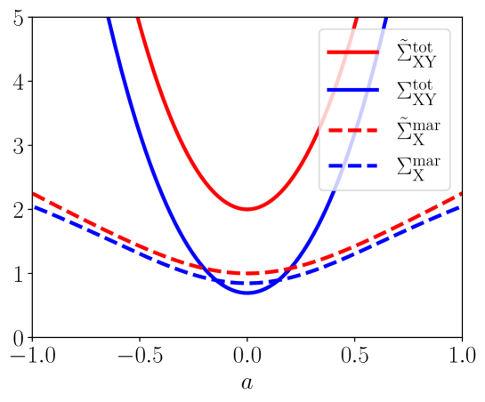
Figure 6: Relationship between total entropy production and marginal entropy production for Gaussian process.

6 Summary and Discussion

6.1 Summary

In this paper, we discussed entropy production for discrete-time Markov processes. In previous studies of stochastic thermodynamics, the entropy production is often discussed based on a continuous-time master equation. However, considering applications to information-theoretic systems that have been actively studied in recent years, such as neural networks and time-series data analysis, it is necessary to derive formulas for the entropy production for use as a measure of irreversibility in discrete-time stochastic dynamics. However, there have not been many studies of discrete-time systems, these studies have used multiple definitions of entropy production without drawing any distinctions between them. Therefore, in this study, we have explicitly distinguished and discussed the multiple definitions of entropy production that have been used in previous studies of discrete-time Markov processes.

First, we defined backward entropy production and time-reversed entropy production that satisfy the condition of non-negativity in single systems, and we showed that they are equal in the steady state and in the continuous-time limit. We also discussed the implications of backward entropy production and time-reversed entropy production, using a two-dimensional Gaussian distribution as an example. Backward entropy production represents the difference between the posterior distribution and the transition probability of the inverse process at time $t$ based on Bayesian inference, and time-reversed entropy production represents the degree of violation of the detailed balance. Next, we defined backward total entropy production, time-reversed total entropy production, backward partial entropy production, time-reversed partial entropy production, backward marginal entropy production, time-reversed marginal entropy production, backward conditional entropy production, and time-reversed conditional entropy production as properties that satisfy non-negativity in composite systems.

Previous studies have considered various decomposition of entropy production. In this paper, we have provided backward and time-reversed definitions of thermodynamic, information-thermodynamic and information-theoretic decomposition of entropy production. The definitions of thermodynamic and information-thermodynamic decomposition were used to derive inequalities known as the second law of thermodynamics and the second law of information thermodynamics, respectively.

In continuous-time systems, it is known that total entropy production is bounded from below by marginal entropy production. This means that when an experiment is conducted to measure entropy production in a composite system with multiple interacting subsystems, the entropy production calculated only from the data of observable variables is an underestimate of the correct entropy production. Similar inequalities have been derived for discrete-time systems, but no clear distinction has been made as to what definition of entropy production was used. In this paper, we have shown that when the time-reversed definition is adopted, total entropy production is bounded from below by marginal entropy production, but is not necessarily bounded from below when the backward definition is adopted. We also showed that the same magnitude relationship holds for partial entropy production and marginal entropy production.

Finally, as an example, we presented analytical calculations of total entropy production, partial entropy production, and marginal entropy production for Gaussian process and based on these results, we performed numerical calculations of total entropy production and marginal entropy production. The results of these analytical calculations show that total entropy production causes expansion/contraction effects and asymmetric interaction effects due to the interaction of the constituent subsystems of a composite system, but only the effects of asymmetry appear in the setting of numerical computations. We have confirmed that these results are consistent with theory under these conditions.

In summary, due to differences in the definitions of time-reversed entropy production and backward entropy production, it seems that these definitions are applicable to different applications and should be used for different purposes. Since time-reversed entropy production is a measure of the irreversibility of stochastic dynamics in non-equilibrium systems, it is appropriate to use it in situations such as living organisms, which interact strongly with the environment and are thus kept in non-equilibrium states, and where it is necessary to rigorously capture violations of the detailed balance. On the other hand, backward entropy production is a measure that describes how probabilistic dynamics can be viewed as Bayesian inference about the past. It is therefore suitable for statistical time-series analysis and information-theoretic analysis, and is appropriate for time-series dynamics in general, including chemical/biological reactions and social networks, where it is necessary to analyze the flow of information.

6.2 Discussion

This study focused on a Gaussian process as an example, but other systems are worthy of study, including the kinetic Ising model. The kinetic Ising model is mathematically equivalent to a neural network, and can be used to describe neural activity. In an analysis where the mean field approximation is applied to the kinetic Ising model, numerical calculation shows that entropy production is maximized near the phase transition point when the inverse temperature is changed in the steady state [39]. It has been shown that entropy production is maximized in an Ising models driven by periodic external field [40] and majority-vote models [41, 42]. Analytical calculations of entropy production in a kinetic Ising model in the steady state confirm that entropy production is maximized near the phase transition point [43]. These results imply that entropy production is a quantity that characterizes phase transitions in non-equilibrium stochastic dynamics. As described in this paper, backward entropy production and time-reversed entropy production are equivalent in the steady state, but different in non-steady-state conditions. Here, when analyzing neural activity data obtained from active animals, it is necessary to deal with time series that are generally non-stationary, including taking non-steady-state conditions into consideration [44, 45]. It is therefore important to calculate the entropy production of kinetic Ising models in non-steady states for both backward and time-reversed entropy production, and to investigate differences in their behavior. In particular, the maximization for entropy production when the inverse temperature is changed in non-steady state requires investigation.

Another interesting issue is the relationship between the statistical and information-theoretic interdependence of neurons and entropy production in the kinetic Ising model. For example, in two-dimensional kinetic Ising models, previous study discussed the pairwise mutual information between two adjacent neurons and the global mutual information as measures of static dependence between neurons, and the pairwise transfer entropy between two adjacent neurons and the global transfer entropy as measures of dynamic dependence [46]. The results show that the pairwise mutual information, the global mutual information, and the pairwise transfer entropy are maximized at phase transition points, and that the global transfer entropy is maximized in the disordered phase near phase transition points. The behavior of these information quantities near phase transition points resembles the behavior of entropy production near phase transition points. It might be possible to clarify this relationship by analyzing the information-theoretic decomposition of entropy production discussed in section 3.3.

Another challenge is the thermodynamic uncertainty relation (TUR) for discrete-time systems [47, 48]. TUR is an inequality in which entropy production is bounded from below by a function that depends on a quantity called current. This is a tighter inequality than the second law of thermodynamics, and can be used to estimate entropy production [49]. It has been pointed out that TUR does not hold for the steady state in a discrete-time system [50]. Subsequently, looser bounds were derived for time-reversed entropy production [51], and after that, tighter bounds were derived for the steady state [52]. In recent years, an even tighter bound has been derived for backward entropy production [29]. However, these studies made no distinction between time-reversed entropy production and backward entropy production, and their discussions were limited to single systems. For continuous-time systems, TUR in a composite system has already been derived [53, 54], but it is not clear whether TUR holds in a discrete-time composite system in the same way as for a continuous-time composite system. Based on the results of this paper, It might be possible to derive TUR for discrete-time composite systems by drawing distinctions between different definitions of entropy production.

Finally, the challenge of clarifying the Bayesian inference interpretation of entropy production should be addressed. A recent study [55, 56] concluded that it is more natural to interpret the fluctuation theorem as a comparison of forward processes and time-reversed Bayesian inferences, rather than as a comparison of forward and time-reversed processes. However, these studies limited their discussions to the steady state. On the other hand, in this paper, we have shown that for non-stationary states in general, backward entropy production quantifies the difference between the temporal evolution of the forward process and the Bayesian inference of past states, and we have discussed this in relation to time-reversed entropy production. The relationship between these arguments is not clear, therefore it might be worthwhile drawing a clear distinction between backward entropy production and time-reversed entropy production, and providing an interpretation of fluctuation theorem based on Bayesian statistics in the future.

References

- [1] Dilip Kondepudi and Ilya Prigogine. Modern Thermodynamics: From Heat Engines to Dissipative Structures. Wiley, October 2014.
- [2] J. Schnakenberg. Network theory of microscopic and macroscopic behavior of master equation systems. Rev. Mod. Phys., 48(4):571–585, October 1976.
- [3] Ken Sekimoto. Stochastic Energetics. Springer, March 2010.
- [4] Udo Seifert. Stochastic thermodynamics, fluctuation theorems and molecular machines. Rep. Prog. Phys., 75(12):126001, November 2012.
- [5] C. Van den Broeck and M. Esposito. Ensemble and trajectory thermodynamics: A brief introduction. Physica A: Statistical Mechanics and its Applications, 418:6–16, January 2015.
- [6] Juan M. R. Parrondo, Jordan M. Horowitz, and Takahiro Sagawa. Thermodynamics of information. Nature Phys, 11(2):131–139, February 2015.
- [7] Takahiro Sagawa and Masahito Ueda. Generalized Jarzynski Equality under Nonequilibrium Feedback Control. Phys. Rev. Lett., 104(9):090602, March 2010.
- [8] Susanne Still, David A. Sivak, Anthony J. Bell, and Gavin E. Crooks. Thermodynamics of Prediction. Phys. Rev. Lett., 109(12):120604, September 2012.
- [9] Andre C. Barato, David Hartich, and Udo Seifert. Efficiency of cellular information processing. New J. Phys., 16(10):103024, October 2014.
- [10] Rory A. Brittain, Nick S. Jones, and Thomas E. Ouldridge. What we learn from the learning rate. J. Stat. Mech., 2017(6):063502, June 2017.
- [11] Giovanni Diana and Massimiliano Esposito. Mutual entropy production in bipartite systems. J. Stat. Mech., 2014(4):P04010, April 2014.
- [12] Sebastian Goldt and Udo Seifert. Stochastic Thermodynamics of Learning. Phys. Rev. Lett., 118(1):010601, January 2017.
- [13] Sebastian Goldt and Udo Seifert. Thermodynamic efficiency of learning a rule in neural networks. New J. Phys., 19(11):113001, November 2017.
- [14] D. Hartich, A. C. Barato, and U. Seifert. Stochastic thermodynamics of bipartite systems: Transfer entropy inequalities and a Maxwell’s demon interpretation. J. Stat. Mech., 2014(2):P02016, February 2014.
- [15] David Hartich, Andre C. Barato, and Udo Seifert. Sensory capacity: An information theoretical measure of the performance of a sensor. Phys. Rev. E, 93(2):022116, February 2016.
- [16] Jordan M. Horowitz and Massimiliano Esposito. Thermodynamics with Continuous Information Flow. Phys. Rev. X, 4(3):031015, July 2014.
- [17] Jordan M. Horowitz and Henrik Sandberg. Second-law-like inequalities with information and their interpretations. New J. Phys., 16(12):125007, December 2014.
- [18] Takumi Matsumoto and Takahiro Sagawa. Role of sufficient statistics in stochastic thermodynamics and its implication to sensory adaptation. Phys. Rev. E, 97(4):042103, April 2018.
- [19] Pablo Sartori, Léo Granger, Chiu Fan Lee, and Jordan M. Horowitz. Thermodynamic Costs of Information Processing in Sensory Adaptation. PLOS Computational Biology, 10(12):e1003974, December 2014.
- [20] Jordan M. Horowitz. Multipartite information flow for multiple Maxwell demons. J. Stat. Mech., 2015(3):P03006, March 2015.
- [21] S. Ciliberto. Experiments in Stochastic Thermodynamics: Short History and Perspectives. Phys. Rev. X, 7(2):021051, June 2017.
- [22] Rodrigo Cofré and Cesar Maldonado. Information Entropy Production of Maximum Entropy Markov Chains from Spike Trains. Entropy, 20(1):34, January 2018.
- [23] Christopher W. Lynn, Eli J. Cornblath, Lia Papadopoulos, Maxwell A. Bertolero, and Danielle S. Bassett. Broken detailed balance and entropy production in the human brain. PNAS, 118(47), November 2021.
- [24] Édgar Roldán and Juan M. R. Parrondo. Entropy production and Kullback-Leibler divergence between stationary trajectories of discrete systems. Phys. Rev. E, 85(3):031129, March 2012.
- [25] Andrea Auconi, Andrea Giansanti, and Edda Klipp. Information Thermodynamics for Time Series of Signal-Response Models. Entropy, 21(2):177, February 2019.
- [26] Pierre Gaspard. Time-Reversed Dynamical Entropy and Irreversibility in Markovian Random Processes. Journal of Statistical Physics, 117(3):599–615, November 2004.
- [27] Julian Lee. Derivation of Markov processes that violate detailed balance. Phys. Rev. E, 97(3):032110, March 2018.
- [28] Gavin E. Crooks and Susanne Still. Marginal and conditional second laws of thermodynamics. EPL, 125(4):40005, March 2019.
- [29] Kangqiao Liu, Zongping Gong, and Masahito Ueda. Thermodynamic Uncertainty Relation for Arbitrary Initial States. Phys. Rev. Lett., 125(14):140602, September 2020.
- [30] Thomas M. Cover and Joy A. Thomas. Elements of Information Theory. John Wiley & Sons, November 2012.
- [31] Sosuke Ito, Masafumi Oizumi, and Shun-ichi Amari. Unified framework for the entropy production and the stochastic interaction based on information geometry. Phys. Rev. Research, 2(3):033048, July 2020.
- [32] R. Chétrite, M. L. Rosinberg, T. Sagawa, and G. Tarjus. Information thermodynamics for interacting stochastic systems without bipartite structure. J. Stat. Mech., 2019(11):114002, November 2019.
- [33] Kyogo Kawaguchi and Yohei Nakayama. Fluctuation theorem for hidden entropy production. Phys. Rev. E, 88(2):022147, August 2013.
- [34] Sosuke Ito. Backward transfer entropy: Informational measure for detecting hidden Markov models and its interpretations in thermodynamics, gambling and causality. Sci Rep, 6(1):36831, November 2016.
- [35] Thomas Schreiber. Measuring Information Transfer. Phys. Rev. Lett., 85(2):461–464, July 2000.
- [36] R. Kawai, J. M. R. Parrondo, and C. Van den Broeck. Dissipation: The Phase-Space Perspective. Phys. Rev. Lett., 98(8):080602, February 2007.
- [37] Max Welling. The Kalman Filter.
- [38] Kaare Brandt Petersen and Michael Syskind Pedersen. The Matrix Cookbook.
- [39] Miguel Aguilera, S. Amin Moosavi, and Hideaki Shimazaki. A unifying framework for mean-field theories of asymmetric kinetic Ising systems. Nat Commun, 12(1):1197, February 2021.
- [40] Yirui Zhang and Andre C. Barato. Critical behavior of entropy production and learning rate: Ising model with an oscillating field. J. Stat. Mech., 2016(11):113207, November 2016.
- [41] Leonardo Crochik and Tânia Tomé. Entropy production in the majority-vote model. Phys. Rev. E, 72(5):057103, November 2005.
- [42] C. E. Fernández Noa, Pedro E. Harunari, M. J. de Oliveira, and C. E. Fiore. Entropy production as a tool for characterizing nonequilibrium phase transitions. Phys. Rev. E, 100(1):012104, July 2019.
- [43] Miguel Aguilera, Masanao Igarashi, and Hideaki Shimazaki. in preparation.
- [44] Hideaki Shimazaki, Shun-ichi Amari, Emery N. Brown, and Sonja Grün. State-Space Analysis of Time-Varying Higher-Order Spike Correlation for Multiple Neural Spike Train Data. PLOS Computational Biology, 8(3):e1002385, March 2012.
- [45] Christian Donner, Klaus Obermayer, and Hideaki Shimazaki. Approximate Inference for Time-Varying Interactions and Macroscopic Dynamics of Neural Populations. PLOS Computational Biology, 13(1):e1005309, January 2017.
- [46] Lionel Barnett, Joseph T. Lizier, Michael Harré, Anil K. Seth, and Terry Bossomaier. Information Flow in a Kinetic Ising Model Peaks in the Disordered Phase. Phys. Rev. Lett., 111(17):177203, October 2013.
- [47] Andre C. Barato and Udo Seifert. Thermodynamic Uncertainty Relation for Biomolecular Processes. Phys. Rev. Lett., 114(15):158101, April 2015.
- [48] Naoto Shiraishi. Optimal Thermodynamic Uncertainty Relation in Markov Jump Processes. J Stat Phys, 185(3):19, November 2021.
- [49] Shun Otsubo, Sosuke Ito, Andreas Dechant, and Takahiro Sagawa. Estimating entropy production by machine learning of short-time fluctuating currents. Phys. Rev. E, 101(6):062106, June 2020.
- [50] Naoto Shiraishi. Finite-time thermodynamic uncertainty relation do not hold for discrete-time Markov process. arXiv:1706.00892 [cond-mat], June 2017.
- [51] Karel Proesmans and Christian Van den Broeck. Discrete-time thermodynamic uncertainty relation. EPL, 119(2):20001, July 2017.
- [52] Davide Chiuchiù and Simone Pigolotti. Mapping of uncertainty relations between continuous and discrete time. Phys. Rev. E, 97(3):032109, March 2018.
- [53] David H. Wolpert. Uncertainty Relations and Fluctuation Theorems for Bayes Nets. Phys. Rev. Lett., 125(20):200602, November 2020.
- [54] Gülce Kardeş and David H. Wolpert. Thermodynamic Uncertainty Relations for Multipartite Processes. arXiv:2101.01610 [cond-mat], March 2021.
- [55] Francesco Buscemi and Valerio Scarani. Fluctuation theorems from Bayesian retrodiction. Phys. Rev. E, 103(5):052111, May 2021.
- [56] Clive Cenxin Aw, Francesco Buscemi, and Valerio Scarani. Fluctuation theorems with retrodiction rather than reverse processes. AVS Quantum Sci., 3(4):045601, December 2021.
- [57] Ying-Jen Yang and Hong Qian. Unified formalism for entropy production and fluctuation relations. Phys. Rev. E, 101(2):022129, February 2020.