Simple Hard Instances for Low-Depth Algebraic Proofs

Abstract

We prove super-polynomial lower bounds on the size of propositional proof systems operating with constant-depth algebraic circuits over fields of zero characteristic. Specifically, we show that the subset-sum variant $\sum_{i,j,k,\ell\in[n]}z_{ijk\ell}x_{i}x_{j}x_{k}x_{\ell}-\beta=0$, for Boolean variables, does not have polynomial-size IPS refutations where the refutations are multilinear and written as constant-depth circuits.

Andrews and Forbes (STOC’22) established recently a constant-depth IPS lower bound, but their hard instance does not have itself small constant-depth circuits, while our instance is computable already with small depth-2 circuits.

Our argument relies on extending the recent breakthrough lower bounds against constant-depth algebraic circuits by Limaye, Srinivasan and Tavenas (FOCS’21) to the functional lower bound framework of Forbes, Shpilka, Tzameret and Wigderson (ToC’21), and may be of independent interest. Specifically, we construct a polynomial $f$ computable with small-size constant-depth circuits, such that the multilinear polynomial computing $\nicefrac{{1}}{{f}}$ over Boolean values and its appropriate set-multilinear projection are hard for constant-depth circuits.

1 Introduction

Proof complexity predominantly aims to establish lower bounds on proof size in different proof systems. From the perspective of complexity theory this can be viewed as the dual goal to circuit complexity. While circuit complexity aims to prove lower bounds on minimal circuit size required to decide membership in certain languages, e.g., SAT, proof complexity aims to establish lower bounds on the minimal size of proofs witnessing membership in a certain language, e.g., UNSAT, the language of unsatisfiable Boolean formulas. Here a proof is simply a witness that can be checked efficiently.

In circuit complexity it is usual to consider different or restricted types of circuits (e.g., constant-depth circuits or constant-depth circuits with counting gates modulo a prime). Similarly, in proof complexity it is standard to consider different or restricted types of proof systems, for example proofs using a prescribed set of inference rules that derive clauses from existing ones (i.e., resolution).

The ideal goal of circuit complexity is to prove that the class $\mathsf{NP}$ is different from the class of languages decidable by polynomial-size circuits (and hence ${\mathsf{NP}}\neq{\mathsf{P}}/{\mathsf{poly}}$). Similarly, the overarching view of proof complexity is that of an attempt to prove lower bounds on stronger and stronger proof systems in the hope to get as close as possible to ruling out the existence of any proof system that admits short proofs for all unsatisfiable formulas (namely, membership in UNSAT; and similarly for proving membership in other important languages). A language that admits no short efficiently verifiable proofs is by definition outside the class $\mathsf{NP}$, from which we conclude, in the case of ruling out short proofs of UNSAT, that ${\mathsf{NP}}\neq{\mathsf{coNP}}$ (and hence ${\mathsf{NP}}\neq{\mathsf{P}}$). This view of proof complexity is usually called The Cook’s Programme of proof complexity.

1.1 Algebraic Proof Systems

One important strand of proof complexity deals with algebraic proof systems of increasing strength. Algebraic proof systems prove that a set of multivariate polynomials do not have a common 0-1 root over a field. The arguably canonical algebraic proof system is the relatively weak Polynomial Calculus (PC for short) [6] in which proofs start from a set of polynomial equations, and proceed to add and multiply existing polynomials until one reaches the unsatisfiable equation $1=0$ (proving that the initial polynomials do not have a common 0-1 solution). The “static” version of the polynomial calculus is called Nullstellensatz [4]. In Nullstellensatz a proof of the unsatisfiability of a set of axioms, given as polynomial equations $\{f_{i}({\overline{x}})=0\}$ over a field, is simply a single polynomial combination of the axioms that equals 1 as a formal polynomial, namely:

$$\sum_{i}g_{i}({\overline{x}})\cdot f_{i}({\overline{x}})=1\,,$$ (1)

for some polynomials $\{g_{i}({\overline{x}})\}$ (it is said to be static because the proof is given as a single polynomial combination instead of deriving 1 “dynamically” step-by-step as in PC).

The size-complexity of proofs in both PC and Nullstellensatz is sparsity, namely the total number of monomials in all the polynomials appearing along the proof. The sparsity measure is what makes these proof systems weak (e.g., even a simple proof-line like $(x_{1}-1)\cdots(x_{n}-1)=0$ accounts for an exponential size because the number of monomials in it is $2^{n}$).

While counting the total number of monomials in algebraic proofs towards their size-complexity yields comparatively weak proof systems, it is natural to think of stronger algebraic proofs by representing polynomials in a more compact manner than sparsity. In particular, one can consider writing polynomials using algebraic circuits. This idea has circulated in proof complexity starting from Pitassi [18, 19], and subsequently in Grigoriev and Hirsch [10], Raz and Tzameret [22, 21, 27], and finally in the introduction of the Ideal Proof System (IPS) by Grochow and Pitassi [9] which loosely speaking is the Nullstellensatz proof system in which proofs are written as algebraic circuits (indeed, [8] showed that IPS is equivalent to Nullstellensatz in which the polynomials $g_{i}$ in Equation 1 are written as algebraic circuits).

Accordingly, it is natural to consider proof systems that sit between the weak Nullstellensatz on the one end and the strong IPS on the other end. This is done by writing polynomials in proofs with restricted kind of algebraic circuits, such as constant-depth circuits [10, 9, 12, 3], noncommutative formulas [27, 16, 27], algebraic branching programs [27, 8, 15], multilinear formulas [22, 21, 8] and very recently algebraic proofs with additional extension variables over large fields [1] or finite fields [13].

1.2 State of the Art in Algebraic Proof-Size Lower Bounds

For the weaker end of the algebraic proof systems’ hierarchy many size lower bounds are known. Beginning in the works of Beame et al. [4] and Buss et al. [5] on Nullstellensatz, through the first Polynomial Calculus (PC) lower bound by Razborov [23], and the PC subset-sum lower bound by Impagliazzo, Pudlak and Sgall [14] (the simplest form of the subset sum principle, also called sometimes Knapsack, is the unsatisfiable over 0-1 values equation $\sum_{i=1}^{n}x_{i}-\beta=0$, for $\beta>n$), as well as many other results.

Only recently, lower bounds against stronger algebraic proof systems were established. Forbes, Shpilka, Tzameret and Wigderson [8] considered subsystems of IPS using read-once oblivious algebraic programs (roABP) and multilinear formulas over large fields. However these subsystems are not necessarily comparable with constant-depth fragments of IPS which are the focus of the current work.

Alekseev [1] established lower bounds against the Polynomial Calculus with additional extension variables (i.e., variables that abbreviate polynomials with a single fresh variable) over large fields. This result is quite strong, since the proof system simulates strong propositional-logic systems like extended Frege. However, this proof system is (apparently) weaker than IPS. Furthermore, the complexity of proofs in this system is measured by bit-size (i.e., coefficients of monomials in each proof-line are written using binary notation; hence, even a short proof using a small number of steps can incur an exponential blow-up if it uses coefficients of super-exponential magnitude, as shown by Alekseev). Lastly, the hard instance in [1] uses coefficients of exponential magnitude, and this is crucial to the lower bound argument.

Very recently, Impagliazzo, Mouli and Pitassi [13] established lower bounds against PC with restricted number of extension variables over finite fields for CNF formulas. However this proof system is apparently weaker (or incomparable to) constant-depth IPS, and is weaker than PC with proof-lines written as constant-depth circuits, because of the restriction on the number of allowed extension variables.

The following lower bounds form the frontiers of what is known about the complexity of strong algebraic proof systems most relevant to our work (i.e., IPS of increasing depth, beginning from Nullstellensatz, which is equivalent to depth-2 IPS, up to unbounded depth IPS):

1. Conditional lower bounds against IPS proofs for the Binary Value Principle $\sum_{i=1}^{n}2^{i-1}x_{i}=-1$ (a subset sum instance with coefficients of exponential magnitude) by Alekseev, Hirsch, Grigoriev and Tzameret [2]. Apart from this result being conditional, the hard instances use coefficients of exponential magnitude, and this is crucial to the lower bound argument.

2. Andrews and Forbes [3] very recently proved constant-depth IPS lower bounds. However, the hard instance itself cannot be computed by a polynomial-size constant-depth circuit, and this fact is crucial to the lower bound proof.

1.3 Our Results

We establish super-polynomial constant-depth IPS lower bounds for a subset sum instance with small coefficients (i.e., 0-1 coefficients) that is computable by an $O(n^{5})$-size depth-2 circuits, and where the IPS proof is multilinear.

To understand better the proof system we work against, recall the proof shown in Equation 1, in which the $g_{i}$’s are written as algebraic circuits—this is (equivalent) to the general IPS system. We shall work with the proof system multilinear $\textup{IPS}_{\text{LIN}^{\prime}}$, following the notation $\textup{IPS}_{\text{LIN}^{\prime}}$ in [8]. Proofs in multilinear $\textup{IPS}_{\text{LIN}^{\prime}}$ of the unsatisfiability of $\{f_{i}({\overline{x}})=0\}$ are (roughly; the actual proof system is in fact stronger than this, see 2) defined as the following polynomial identity

$$\sum_{i}g_{i}({\overline{x}})\cdot f_{i}({\overline{x}})+\sum_{j}h_{j}({\overline{x}})\cdot(x_{j}^{2}-x_{j})=1$$

where $h_{j}({\overline{x}})$ are some polynomials and the $g_{i}({\overline{x}})$’s are multilinear polynomials, and the $g_{i}({\overline{x}})$’s and $h_{j}({\overline{x}})$’s are all written with constant-depth circuits (but not necessarily multilinear formulas, in contrast to multilinear-formula $\textup{IPS}_{\text{LIN}^{\prime}}$ as in [8]).

Theorem 1 (Informal; see Theorem 3).

Every constant-depth multilinear $\textup{IPS}_{\text{LIN}^{\prime}}$ refutation of the subset sum variant $\sum_{i,j,k,\ell\in[n]}z_{ijk\ell}x_{i}x_{j}x_{k}x_{\ell}-\beta$ (for $\beta\not\in\{0,\dots,n^{4}\}$) requires super-polynomial (in $n$) size.

Significance of the Results and Context.

This is the first constant-depth IPS lower bound on an instance that is computable itself with small constant-depth circuits, when the polynomial that constitutes the IPS proof is multilinear (see 2). Our hard instance has coefficients of small magnitude, and the lower bound is in the stronger unit cost model of algebraic circuits (i.e., in terms of the size of the circuits, not the size of the binary representation of the coefficients appearing in them). Thus, we rectify all the purported shortcomings of previous constant-depth algebraic proofs lower bounds (while paying by requiring that the IPS proofs are (partially) multilinear).

Theorem 1 contributes to the tradition of showing that simple subset sum variants are hard for algebraic proofs. While Impagliazzo et al. [14] initially showed that the subset sum principle requires exponentially many monomials in PC refutations, and Forbes et al. [8] extended this to roABP and multilinear formulas, we show this hardness holds at least up to constant-depth IPS (when the proofs are multilinear).

Subset sum variants are not translations of CNF formulas or Boolean formulas more generally. Hence, algebraic-proofs lower bounds for them do not imply (immediately at least) propositional logic proof size lower bounds (i.e., Frege-style proofs). However, a major motivation behind investigating the complexity of algebraic proof systems is to understand the power of algebraic reasoning and proofs (and their algorithmic counterpart, e.g., Gröbner basis computations). For this purpose, it is enough to prove lower bounds on hard instances that are not necessarily translations of CNFs or Boolean formulas. Indeed many works on the complexity of algebraic proof systems are dedicated to establishing such lower bounds, most prominently the subset sum principle, and its variants (see also Razborov [23] non-CNF pigeonhole principle).

Furthermore, lower bounds on the size of algebraic proofs of subset-sum instances, and generally instances from the language of unsatisfiable 0-1 multivariate polynomials over a field, are as relevant to the Cook’s programme mentioned above as much as Boolean formulas. The reason is that this language is a $\mathsf{coNP}$-complete language, since we can efficiently check if a given 0-1 assignment satisfies all the polynomials in the system (assuming the polynomials and field elements are written in some standard way), and Boolean unsatisfiability is easily reducible to this language.

We explain in what follows our main technical contribution, which can be of independent interest.

1.4 Proof Technique

Our proof draws techniques from two sources. We use the methods presented in Limaye, Srinivasan and Tavenas [17] to prove superpolynomial lower bounds for constant-depth algebraic circuits, and combine these with the functional lower bound framework of Forbes, Shpilka, Tzameret and Wigderson [8] for size lower bounds on IPS proofs (see also [FKS16] for the functional lower bound approach in algebraic circuit complexity in general).

In general, we prove Theorem 1 by reducing the task of lower bounding the size of a constant-depth algebraic circuit computing the multilinear polynomial that constitutes the IPS proof into the following task: lower bound the size of a constant-depth set-multilinear circuit computing an associated set-multilinear polynomial. To get the new associated set-multilinear polynomial from the original multilinear IPS proof (which is not necessarily set-multilinear by itself) we use a variant of the functional lower bound approach with some additional arguments that we introduce to deal with the need to focus on set-multilinear monomials within a polynomial that is not set-multilinear.

Once, we have the associated set-multilinear polynomial we can use the reduction presented in [17] from constant-depth general circuits to constant-depth set-multilinear circuits. The reduction loses only a constant-factor in the depth, but pays quite heavily in the degree of the set-multilinear output polynomial. So in order to keep the size of the obtained set-multilinear circuit reasonable, we need to restrict the degree of the set-multilinear polynomial considerably.

Notice that unlike in Limaye et al. [17] (or in circuit complexity in general), we do not work from the get-go with a set-multilinear polynomial for which we need to prove a lower bound against constant-depth circuits computing it. In our case, we need to somehow show that this set-multilinear polynomial is “embedded” in some way in any multilinear IPS proof of our hard instance. This is the main technical challenge we face in this work.

Another point is that to show our simple degree-2 instance from Theorem 1 is hard we use a substitution in this simple instance. Specifically, by assigning some of the $z_{ijk\ell}$ and $x_{i}$ variables in the hard instance, we show that one gets another variant of subset sum denoted $\mathsf{ks}_{w}$ ($\mathsf{ks}$ stands for Knapsack) that is defined with respect to some word $w\in\mathbb{Z}^{d}$ (in the sense of [17]). The definition of the subset sum over $w$ is designed so that the multilinear IPS refutation of the simple hard instance from Theorem 1 “embeds” $P_{w}$ after applying the substitution to the $z_{ijk\ell}$ (and $x_{i}$) variables, where $P_{w}$ is the word polynomial from [17], which induces a full-rank coefficient matrix on a set of all set-multilinear monomials that arise from the given word $w$ (a coefficient matrix of a polynomial is an associated matrix whose rank serves as a complexity measure for the polynomial’s circuit size, and in which each entry is a coefficient of a specific monomial in the polynomial).

The meaning of a polynomial “embedding” a set-multilinear polynomial refers to the set-multilinear polynomial being the set-multilinear projection of the original polynomial. Hence, we need to consider the projection to the space of all set-multilinear polynomials over a particular variable-partition of our original polynomial. We extend the evaluation dimension method from [8] to prove a rank lower bound for the coefficient matrix of this set-multilinear projection, which yields the set-multilinear circuit lower bound via a lemma from [17].

To add on the above, our proof diverges from its forbears in some essential ways. Firstly, as mentioned before, when [17] can work from the get-go with a low-degree set-multilinear polynomial, the multilinear refutations we consider are not of low-degree nor are they set-multilinear. Thus we need to find suitable set-multilinear polynomials within the refutations, and consider projections to the space of set-multilinear polynomials with respect to some variable-partition. Secondly, we use the method based on partial assignments (or evaluations) from [8] to prove our rank lower bound. Our use of these partial assignments is however more subtle than the evaluation dimension method of [8].

Forbes et al. [8] showed a rank lower bound against a coefficient matrix of a polynomial by reducing it to dimension lower bound for the space of all multilinearizations of the polynomials obtained after appropriate partial assignments (to the ${\overline{y}}$-variables of a polynomial in both ${\overline{x}}$ and ${\overline{y}}$ variables; see [8]). The dimension lower bound is then proved by showing that enough linearly independent monomials appear in the space as leading monomials. Such an argument is not enough in our case, because we need to prove the existence of specific set-multilinear monomials (with respect to to a words $w$) in the original polynomial (namely, the IPS proof polynomial). The root of this difference is that the original argument defines partial assignments over all the monomials in the hard polynomial, while we try to argue for a rank lower bound for the coefficient matrix of only a part of the monomials, namely only the set-multilinear monomials within a non-set-multilinear polynomial—and this corresponds to only a submatrix of the full coefficient matrix. The drawback here is that this also forces us to consider only multilinear refutations (because multilinearization as used in [8] does not increase rank but preserves the high rank of the coefficient matrix of the original polynomial [before multilinearization], while multilinearization of a polynomial can increase the rank of the set-multilinear coefficient sub-matrix; e.g., multilinearizing the non-set-multilinear monomial $x^{2}_{1}y_{2}^{3}$ produces $x_{1}y_{2}$ which is set-multilinear, assuming the variables are partitioned into ${\overline{x}}$ and ${\overline{y}}$ variables).

Note also that our proof technique is completely different from Andrews and Forbes [3] who used the hard multiples framework from [8].

2 Preliminaries

2.1 Polynomials and Algebraic Circuits

For excellent treatises on algebraic circuits and their complexity see Shpilka and Yehudayoff [26] as well as Saptharishi [24]. Let $\mathbb{G}$ be a ring. Denote by $\mathbb{G}[X]$ the ring of (commutative) polynomials with coefficients from $\mathbb{G}$ and variables $X:=\{x_{1},x_{2},\,\dots\,\}$. A polynomial is a formal linear combination of monomials, where a monomial is a product of variables. Two polynomials are identical if all their monomials have the same coefficients.

The (total) degree of a monomial is the sum of all the powers of variables in it. The (total) degree of a polynomial is the maximal total degree of a monomial in it. The degree of an individual variable in a monomial is its power. The individual degree of a monomial is the maximal individual degree of its variables. The individual degree of a polynomial is the maximal individual degree of its monomials. For a polynomial $f$ in $\mathbb{G}[X,Y]$ with $X,Y$ being pairwise disjoint sets of variables, the individual $Y$-degree of $f$ is the maximal individual degree of a $Y$-variable only in $f$.

Algebraic circuits and formulas over the ring $\mathbb{G}$  compute polynomials in $\mathbb{G}[X]$ via addition and multiplication gates, starting from the input variables and constants from the ring. More precisely, an algebraic circuit $C$ is a finite directed acyclic graph (DAG) with input nodes (i.e., nodes of in-degree zero) and a single output node (i.e., a node of out-degree zero). Edges are labelled by ring $\mathbb{G}$ elements. Input nodes are labelled with variables or scalars from the underlying ring. In this work (since we work with constant-depth circuits) all other nodes have unbounded fan-in (that is, unbounded in-degree) and are labelled by either an addition gate $+$ or a product gate $\times$. Every node in an algebraic circuit $C$ computes a polynomial in $\mathbb{G}[X]$ as follows: an input node computes the variable or scalar that labels it. A $+$ gate computes the linear combination of all the polynomials computed by its incoming nodes, where the coefficients of the linear combination are determined by the corresponding incoming edge labels. A $\times$ gate computes the product of all the polynomials computed by its incoming nodes (so edge labels in this case are not needed). The polynomial computed by a node $u$ in an algebraic circuit $C$ is denoted $\widehat{u}$. Given a circuit $C$, we denote by $\widehat{C}$ the polynomial computed by $C$, that is, the polynomial computed by the output node of $C$. The size of a circuit $C$ is the number of nodes in it, denoted $|C|$, and the depth of a circuit is the length of the longest directed path in it (from an input node to the output node). The product-depth of the circuit is the maximal number of product gates in a directed path from an input node to the output node.

We say that a polynomial is homogeneous whenever every monomial in it has the same (total) degree. We say that a polynomial is multilinear whenever the individual degrees of each of its variables are at most 1.

Let $\overline{X}=\langle X_{1},\ldots,X_{d}\rangle$ be a sequence of pairwise disjoint sets of variables, called variable-partition. We call a monomial $m$ in the variables $\bigcup_{i\in[d]}X_{i}$ set-multilinear over the variable-partition $\overline{X}$ if it contains exactly one variable from each of the sets $X_{i}$, i.e. if there are $x_{i}\in X_{i}$ for all $i\in[d]$ such that $m=\prod_{i\in[d]}x_{i}$. A polynomial $f$ is set-multilinear over $\overline{X}$ if it is a linear combination of set-multilinear monomials over $\overline{X}$. For a sequence $\overline{X}$ of sets of variables, we denote by $\mathbb{F}_{\mathrm{sml}}[\overline{X}]$ the space of all polynomials that are set-multilinear over $\overline{X}$.

We say that an algebraic circuit $C$ is set-multilinear over $\overline{X}$ if $C$ computes a polynomial that is set-multilinear over $\overline{X}$, and each internal node of $C$ computes a polynomial that is set-multilinear over some sub-sequence of $\overline{X}$.

2.2 Strong Algebraic Proof Systems

For a survey about algebraic proof systems and their relations to algebraic complexity see the survey [20]. Grochow and Pitassi [11] suggested the following algebraic proof system which is essentially a Nullstellensatz proof system ([4]) written as an algebraic circuit. A proof in the Ideal Proof System is given as a single polynomial. We provide below the Boolean version of IPS (which includes the Boolean axioms), namely the version that establishes the unsatisfiability over 0-1 of a set of polynomial equations. In what follows we follow the notation in [8]:

Definition 2 (Ideal Proof System (IPS), Grochow-Pitassi [11]).

Let $f_{1}({\overline{x}}),\ldots,f_{m}({\overline{x}}),p({\overline{x}})$ be a collection of polynomials in $\mathbb{F}[x_{1},\ldots,x_{n}]$ over the field $\mathbb{F}$. An IPS proof of $p({\overline{x}})=0$ from axioms $\{f_{j}({\overline{x}})=0\}_{j=1}^{m}$, showing that $p({\overline{x}})=0$ is semantically implied from the assumptions $\{f_{j}({\overline{x}})=0\}_{j=1}^{m}$ over $0$-$1$ assignments, is an algebraic circuit $C({\overline{x}},{\overline{y}},{\overline{z}})\in\mathbb{F}[{\overline{x}},y_{1},\ldots,y_{m},z_{1},\ldots,z_{n}]$ such that (the equalities in what follows stand for formal polynomial identities):

1. $C({\overline{x}},{\overline{0}},{\overline{0}})=0$; and

2. $C({\overline{x}},f_{1}({\overline{x}}),\ldots,f_{m}({\overline{x}}),x_{1}^{2}-x_{1},\ldots,x_{n}^{2}-x_{n})=p({\overline{x}})$.

The size of the IPS proof is the size of the circuit $C$. An IPS proof $C({\overline{x}},{\overline{y}},{\overline{z}})$ of $1=0$ from $\{f_{j}({\overline{x}})=0\}_{j\in[m]}$ is called an IPS refutation of $\{f_{j}({\overline{x}})=0\}_{j\in[m]}$ (note that in this case it must hold that $\{f_{j}({\overline{x}})=0\}_{j=1}^{m}$ have no common solutions in $\{0,1\}^{n}$). If $\widehat{C}$ (the polynomial computed by $C$) is of individual degree $\leq 1$ in each $y_{j}$ and $z_{i}$, then this is a linear IPS refutation (called Hilbert IPS by Grochow-Pitassi [9]), which we will abbreviate as IPS${}_{\textup{LIN}}$. If $\widehat{C}$ is of individual degree $\leq 1$ only in the $y_{j}$’s then we say this is an $\textup{IPS}_{\text{LIN}^{\prime}}$ refutation (following [8]). If $\widehat{C}({\overline{x}},{\overline{y}},{\overline{0}})$ is of individual degree $\leq 1$ in each $x_{j}$ and $y_{i}$ variables, while $\widehat{C}({\overline{x}},{\overline{0}},{\overline{z}})$ is not necessarily multilinear, then this is a multilinear $\textup{IPS}_{\text{LIN}^{\prime}}$ refutation.

If $C$ is of depth at most $d$, then this is called a depth-$d$ IPS refutation, and further called a depth-$d$ IPS${}_{\textup{LIN}}$ refutation if $\widehat{C}$ is linear in ${\overline{y}},{\overline{z}}$, and a depth-$d$ $\textup{IPS}_{\text{LIN}^{\prime}}$ refutation if $\widehat{C}$ is linear in ${\overline{y}}$, and depth-$d$ multilinear $\textup{IPS}_{\text{LIN}^{\prime}}$ refutation if $\widehat{C}({\overline{x}},{\overline{y}},{\overline{0}})$ is linear in ${\overline{x}},{\overline{y}}$.

Notice that the definition above adds the equations $\{x_{i}^{2}-x_{i}=0\}_{i=1}^{n}$, called the Boolean axioms denoted ${\overline{x}}^{2}-{\overline{x}}$, to the system $\{f_{j}({\overline{x}})=0\}_{j=1}^{m}$. This allows to refute over $\{0,1\}^{n}$ unsatisfiable systems of equations. The variables ${\overline{y}},{\overline{z}}$ are called the placeholder variables since they are used as placeholders for the axioms. Also, note that the first equality in the definition of IPS means that the polynomial computed by $C$ is in the ideal generated by $\overline{y},\overline{z}$, which in turn, following the second equality, means that $C$ witnesses the fact that $1$ is in the ideal generated by $f_{1}({\overline{x}}),\ldots,f_{m}({\overline{x}}),x_{1}^{2}-x_{1},\ldots,x_{n}^{2}-x_{n}$ (the existence of this witness, for unsatisfiable set of polynomials, stems from the Nullstellensatz theorem [4]).

In this work we focus on multilinear $\textup{IPS}_{\text{LIN}^{\prime}}$ refutations. This proof system is complete because its weaker subsystem multilinear-formula $\textup{IPS}_{\text{LIN}^{\prime}}$  was shown in [8, Corollary 4.12] to be complete (and to simulate Nullstellensatz with respect to sparsity by already depth-2 multilinear $\textup{IPS}_{\text{LIN}^{\prime}}$ proofs).

To build an intuition for multilinear $\textup{IPS}_{\text{LIN}^{\prime}}$ it is useful to consider a subsystem of it in which refutations are written as

$$C({\overline{x}},{\overline{y}},{\overline{z}})=\sum_{i}g_{i}({\overline{x}})\cdot y_{i}+C^{\prime}({\overline{x}},{\overline{z}}),$$

where $\widehat{C}^{\prime}({\overline{x}},{\overline{0}})=0$ and the $\widehat{g}_{i}$’s are multilinear. Note indeed that $C({\overline{x}},{\overline{0}},{\overline{0}})=0$ so that the first condition of IPS proofs holds, and that $C({\overline{x}},{\overline{y}},{\overline{0}})$ is indeed multilinear in ${\overline{x}},{\overline{y}}$.

Important remark: Unlike the multilinear-formula $\textup{IPS}_{\text{LIN}^{\prime}}$ in [8], in multilinear $\textup{IPS}_{\text{LIN}^{\prime}}$ refutations $C({\overline{x}},{\overline{y}},{\overline{z}})$ we do not require that the refutations are written as multilinear formulas or multilinear circuits, only that the polynomial computed by $C({\overline{x}},{\overline{y}},{\overline{0}})$ is multilinear, hence the latter proof system easily simulates the former.

2.3 Set-Multilinear Monomials over a Word

We recall some notation from [17]. Let $w\in\mathbb{Z}^{d}$ be a word. For a subset $S\subseteq[d]$ denote by $w_{S}$ the sum $\sum_{i\in S}w_{i}$, and by $w|_{S}$ the subword of $w$ indexed by the set $S$. Let

$$P_{w}:=\{i\in[d]:w_{i}\geq 0\}$$

be the set of positive indices of $w$ and let

$$N_{w}:=\{i\in[d]:w_{i}<0\}$$

be the set of negative indices of $w$.

Given a word $w$, we associate with it a sequence $\overline{X}(w)=\langle X(w_{1}),\ldots,X(w_{d})\rangle$ of sets of variables, where for each $i\in[d]$ the size of $X(w_{i})$ is $2^{|w_{i}|}$. We call a monomial set-multilinear over a word $w$ if it is set-multilinear over the sequence $\overline{X}(w)$.

For a word $w$, let $\Pi_{w}$ denote the projection onto the space $\mathbb{F}_{\mathrm{sml}}[\overline{X}(w)]$ that maps the set-multilinear monomials over $w$ identically to themselves and all other monomials to $0$.

2.4 Relative Rank

Let $M^{P}_{w}$ and $M^{N}_{w}$ denote the set-multilinear monomials over $w|_{P_{w}}$ and $w|_{N_{w}}$, respectively. Let $f\in\mathbb{F}_{\mathrm{sml}}[\overline{X}(w)]$ and denote by $M_{w}(f)$ the matrix with rows indexed by $M^{P}_{w}$ and columns indexed by $M^{N}_{w}$, whose $(m,m^{\prime})$th entry is the coefficient of the monomial $mm^{\prime}$ in $f$.

For any $f\in\mathbb{F}_{\mathrm{sml}}[\overline{X}(w)]$ define the relative rank with respect to $w$ as follows

$$\mathrm{relrk}_{w}(f)=\frac{\operatorname{rank}(M_{w}(f))}{\sqrt{|M^{P}_{w}|\cdot|M^{N}_{w}|}}.$$

2.5 Monomial Orders

Finally we recall some basic notions related to monomial orders. For an in-depth introduction see [7]. A monomial order (in a polynomial ring $\mathbb{F}[X]$) is a well-order $\leq$ on the set of all monomials that respects multiplication:

$$\text{if }m_{1}\leq m_{2}\text{, then }m_{1}m_{3}\leq m_{2}m_{3}\text{ for any }m_{3}.$$

It is not hard to see that any monomial order extends the submonomial relation: if $m_{1}m_{2}=m_{3}$ for some monomials $m_{1},m_{2}$ and $m_{3}$, then $m_{1}\leq m_{3}$. This is essentially the only property we need of monomial orderings, and thus our results work for any monomial ordering. Given a polynomial $f\in\mathbb{F}[X]$, the leading monomial of $f$, denoted $\operatorname{LM}(f)$, is the highest monomial with respect to $\leq$ that appears in $f$ with a non-zero coefficient.

3 The Lower Bound

Our main theorem is as follows:

Theorem 3 (Main).

Let $n,\Delta\in\mathbb{N}_{+}$ with $\Delta\leq\nicefrac{{1}}{{4}}\log\log\log n$, and assume that $\operatorname{char}(\mathbb{F})=0$. Then any product-depth at most $\Delta$ multilinear $\textup{IPS}_{\text{LIN}^{\prime}}$ refutation of the subset sum variant $\sum_{i,j,k,\ell\in[n]}z_{ijk\ell}x_{i}x_{j}x_{k}x_{\ell}-\beta$ (for $\beta\not\in\{0,\dots,n^{4}\}$) is of size at least $n^{(\log n)^{\exp(-O(\Delta))}}$.

Note that, when $\Delta\geq\omega(\log\log\log n)$, the lower bound above becomes trivial. To prove Theorem 3 we need the following theorem, which is proved in the sequel:

Theorem 4.

Let $n,\Delta\in\mathbb{N}_{+}$ with $\Delta\leq\nicefrac{{1}}{{4}}\log\log\log n$, and assume that $\operatorname{char}(\mathbb{F})=0$. Let $f$ be the multilinear polynomial such that

$$f=\frac{1}{\sum_{i,j,k,\ell\in[n]}z_{ijk\ell}x_{i}x_{j}x_{k}x_{\ell}-\beta}\text{\quad over Boolean assignments.}$$

Then, any circuit of product-depth at most $\Delta$ computing $f$ has size at least

$$n^{(\log n)^{\exp(-O(\Delta))}}\,.$$

Proof of Theorem 3 from Theorem 4.

Let $C({\overline{x}},{\overline{y}},{\overline{w}})$ be a multilinear $\textup{IPS}_{\text{LIN}^{\prime}}$  refutation of $\sum_{i,j,k,\ell\in[n]}z_{ijk\ell}x_{i}x_{j}x_{k}x_{\ell}-\beta=0$ (where here for notational clarity we renamed the Boolean axioms placeholder variables from ${\overline{z}}$ to ${\overline{w}}$). Since there is only one non-Boolean axiom, $C$ has in fact only a single ${\overline{y}}$ variable denoted $y$ (i.e., ${\overline{y}}=\{y\}$). Note that $\widehat{C}({\overline{x}},y,{\overline{0}})=g({\overline{x}})\cdot y$, for some polynomial $g({\overline{x}})\in\mathbb{F}[{\overline{x}}]$, because by assumption $\widehat{C}$ is linear in the ${\overline{y}}$ variables (and since $\widehat{C}({\overline{x}},0,{\overline{0}})=0$). Therefore, $C({\overline{x}},1,{\overline{0}})$ computes the polynomial $g({\overline{x}})$. Thus, the minimal product-depth-$\Delta$ circuit-size of $g({\overline{x}})$ lower bounds the minimal product-depth-$\Delta$ circuit-size of $C({\overline{x}},y,{\overline{w}})$. It remains to lower bound the size of product depth at most $\Delta$ circuits computing $g({\overline{x}})$.

Notice first that

$$\widehat{C}({\overline{x}},y,{\overline{w}})=\widehat{C}({\overline{x}},y,{\overline{0}})+\sum_{i}h_{i}\cdot w_{i},$$

for some polynomials $h_{i}$ in ${\overline{x}},y,{\overline{w}}$. Thus, $\widehat{C}({\overline{x}},y,{\overline{w}})=g({\overline{x}})\cdot y+\sum_{i}h_{i}\cdot w_{i}$.

By definition of an IPS refutation

$$\widehat{C}\left({\overline{x}},\sum_{i,j,k,\ell\in[n]}z_{ijk\ell}x_{i}x_{j}x_{k}x_{\ell}-\beta,{\overline{x}}^{2}-{\overline{x}}\right)=1$$

and so

$$g({\overline{x}})\cdot\left(\sum_{i,j,k,\ell\in[n]}z_{ijk\ell}x_{i}x_{j}x_{k}x_{\ell}-\beta\right)+\sum_{i}(h_{i}\cdot(x_{i}^{2}-x_{i}))=1.$$

From this we get that over the Boolean cube $g({\overline{x}})\cdot\sum_{i,j,k,\ell\in[n]}z_{ijk\ell}x_{i}x_{j}x_{k}x_{\ell}-\beta\equiv 1$ (as a function, not necessarily as a polynomial identity), and hence $g({\overline{x}})=\frac{1}{\sum_{i,j,k,\ell\in[n]}z_{ijk\ell}x_{i}x_{j}x_{k}x_{\ell}-\beta}$ over the Boolean cube. This shows that the size of $C({\overline{x}},y,{\overline{w}})$ must be at least $n^{(\log n)^{\exp(-O(\Delta))}}$ by Theorem 4. ∎

The rest of section 3 is devoted to proving Theorem 4.

We shall use the tight degree lower bound proved in [8] for functions defined by $\hat{f}({\overline{x}})=\nicefrac{{1}}{{f({\overline{x}})}}$ for simple polynomials $f({\overline{x}})$. Specifically, we use the fact that any multilinear polynomial agreeing with $\nicefrac{{1}}{{f({\overline{x}})}}$, where $f({\overline{x}})$ is the subset-sum axiom $\sum_{i=1}^{n}x_{i}-\beta$ (where $\beta$ is such that the axiom has no Boolean roots) must have degree $n$. We note that a degree lower bound of ${\lceil{\nicefrac{{n}}{{2}}}\rceil}+1$ was established by Impagliazzo, Pudlák, and Sgall [14]. However, similar to [8], we need the tight bound of $n$ here as it will be used crucially in the proof of 6 to obtain the rank lower bound, which is a stronger notion than degree lower bound. Recall the notation ${\overline{x}}^{2}-{\overline{x}}$ for the Boolean axioms of the ${\overline{x}}$-variables.

Lemma 5 (Proposition 5.3 in [8]).

Let $n\geq 1$ and $\mathbb{F}$ be a field with $\operatorname{char}(\mathbb{F})>n$ (or $\operatorname{char}(\mathbb{F})=0$). Suppose that $\beta\in\mathbb{F}\setminus\{0,\ldots,n\}$. Let $f\in\mathbb{F}[x_{1},\ldots,x_{n}]$ be a multilinear polynomial such that

$$f({\overline{x}})\left(\sum_{i}x_{i}-\beta\right)=1\mod{\overline{x}}^{2}-{\overline{x}}\;.$$

Then $\deg f=n$.

3.1 Subset-Sum Based on a Word $w$

In this section we define an auxiliary polynomial we use to prove Theorem 4. It is a variant of the subset-sum that is defined from a given word $w$. Let $w\in\mathbb{Z}^{d}$ be arbitrary word, and consider the sequence $\overline{X}(w)=\langle X(w_{1}),\dots,X(w_{d})\rangle$ of sets of variables. We fix now a useful representation of the variables in $\overline{X}(w)$.

For any $i\in P_{w}$, we write the variables of $X(w_{i})$ in the form $x^{(i)}_{\sigma}$, where $\sigma$ is a binary string indexed by the set (formally, a binary string indexed by a set $A$ is a function from $A$ to $\{0,1\}$):

$$A_{w}^{(i)}:=\left[\sum_{\begin{subarray}{c}i^{\prime}\in P_{w}\\ i^{\prime}<i\end{subarray}}w_{i^{\prime}}+1,\sum_{\begin{subarray}{c}i^{\prime}\in P_{w}\\ i^{\prime}\leq i\end{subarray}}w_{i^{\prime}}\right].$$

Hence, the size of $A_{w}^{(i)}$ is precisely $w_{i}$ and binary strings on the interval $A_{w}^{(i)}$ (i.e., $\{0,1\}^{A_{w}^{(i)}}$), allows $2^{|A_{w}^{(i)}|}=2^{w_{i}}$ possible strings, each corresponds to a different variable in $X(w_{i})$.

Similarly, for any $j\in N_{w}$, we write the variables of $X(w_{i})$ in the form $y^{(j)}_{\sigma}$, where $\sigma$ is a binary string indexed by the set

$$B_{w}^{(j)}:=\left[\sum_{\begin{subarray}{c}j^{\prime}\in N_{w}\\ j^{\prime}<j\end{subarray}}|w_{j^{\prime}}|+1,\sum_{\begin{subarray}{c}j^{\prime}\in N_{w}\\ j^{\prime}\leq j\end{subarray}}|w_{j^{\prime}}|\right].$$

We call the variables in $x^{(i)}_{\sigma}$ the positive variables, or simply ${\overline{x}}$-variables, and the variables $y^{(j)}_{\sigma}$ the negative variables, or simply ${\overline{y}}$-variables. We write $A_{w}^{S}$ for the set $\bigcup_{i\in S}A_{w}^{(i)}$ for any $S\subseteq P_{w}$, and $B_{w}^{T}$ for the set $\bigcup_{j\in T}B_{w}^{(j)}$ for any $T\subseteq N_{w}$.

Each monomial that is set-multilinear on $w|_{S}$ for some $S\subseteq P_{w}$ corresponds to a binary string indexed by the set $A_{w}^{S}$, and any monomial that is set-multilinear on $w|_{T}$ for some $T\subseteq N_{w}$ corresponds to a binary string indexed by the set $B_{w}^{T}$. For any set-multilinear monomial $m$ on some $w|_{S}$ with $S\subseteq P_{w}$ we denote by $\sigma(m)$ the corresponding binary string indexed by $A_{w}^{S}$, and for any binary string $\sigma$ indexed by $A_{w}^{S}$ we denote by $m(\sigma)$ the monomial it defines, and similarly for strings and monomials on the negative variables. Thus notice that for a (negative or positive) monomial $m$ we have $m(\sigma(m))=m$. Moreover, if $m$ is a negative monomial and $S\subseteq P_{w}$, we write $m(\sigma(m)|_{A^{S}_{w}})$ to denote the positive monomial determined by the string $\sigma(m)|_{A^{S}_{w}}$ which is a substring of $\sigma(m)$ restricted to $A^{S}_{w}$.

Therefore, every set-multilinear monomial on $w$ is of degree $d$ with each ${\overline{x}}$-variable picked uniquely from the $X(w_{i})$-variables, for $i\in P_{w}$ the positive indices in $w$, and each ${\overline{y}}$-variable is picked uniquely from the $X(w_{j})$-variables, for $j\in N_{w}$ the negative indices in $w$, and moreover the monomial corresponds to a binary string of length $\sum_{i=1}^{d}|w_{i}|$.

We call the word $w$ balanced if for every $i\in P_{w}$ there is some $j\in N_{w}$ such that $A_{w}^{(i)}\cap B_{w}^{(j)}\neq\emptyset$ and for every $j\in N_{w}$ there is some $i\in P_{w}$ such that $A_{w}^{(i)}\cap B_{w}^{(j)}\neq\emptyset$. This means that any positive variable as defined above has some overlap with some negative variable within the given indexing scheme, and vice versa. Figure 1 and Figure 2 give examples of unbalanced and balanced words, respectively.

Our notion of a balanced word is different from, but related to, the notion of a $b$-unbiased word in [17]: a word $w\in\mathbb{Z}^{d}$ is $b$-unbiased if $|w_{[t]}|\leq b$ for every $t\leq d$. If a balanced word $w\in\mathbb{Z}^{d}$ has all its entries bounded by $b$ in absolute value, i.e., $|w_{i}|\leq b$ for every $i\in[d]$, then the sum of all entries of $w$ is bounded by $b$ in the sense that $|w_{[d]}|\leq b$. The notion of balance is more relaxed than that of unbiased in the sense that we do not need the property that all initial segments are also bounded by $b$. On the other hand the construction and proof in [17] does not require a balanced word, when this property is essential for us in the proof of 6.

Figure 1: An example of an unbalanced word $w\in\mathbb{Z}^{d}$, and where each $w_{i}$ is written as a box with its corresponding binary string index set inside it, such that $|A_{w}^{(i)}|=w_{i}$ for $i\in P_{w}$ and $|B_{w}^{(j)}|=w_{j}$ for $j\in N_{w}$. A word is balanced if for every positive box $i\in P_{w}$, there exists some overlapping negative box, i.e., a $j\in N_{w}$ such that $A_{w}^{(i)}\cap B_{w}^{(j)}\neq\emptyset$, and vice versa. Here however, $B_{w}^{(8)}\cap(A_{w}^{(2)}\cup A_{w}^{(5)}\cup A_{w}^{(6)})=\emptyset$.

Figure 2: An example of a balanced word. The construction of the knapsack polynomial $\textbf{ks}_{w}$ makes use of a balanced word $w$.

We define the polynomial $\mathsf{ks}_{w}$ as follows. Below we suppose that $|w_{N_{w}}|\geq|w_{P_{w}}|$, so that the negative monomials are determined by a longer binary string than the positive ones. Otherwise we flip the roles of the negative and positive variables in the definition below.

For a positive index $i\in P_{w}$ and $\sigma\in\{0,1\}^{A_{w}^{(i)}}$, define the polynomial

$$f^{(i)}_{\sigma}:=\prod_{\begin{subarray}{c}j\in N_{w}:\\ A_{w}^{(i)}\cap B_{w}^{(j)}\neq\emptyset\end{subarray}}\sum_{\sigma_{j}\in\{0,1\}^{B_{w}^{(j)}}}y^{(j)}_{\sigma_{j}},$$ (2)

where the sum ranges over all those $\sigma_{j}$ that agree with $\sigma$ on $A_{w}^{(i)}\cap B_{w}^{(j)}$. The degree of $f^{(i)}_{\sigma}$ equals the number of those $B_{w}^{(j)}$ that overlap with $A_{w}^{(i)}$. Note that the degree is always at least $1$. Now define the polynomial

$$\mathsf{ks}_{w}:=\sum_{i\in P_{w}}\sum_{\sigma\in\{0,1\}^{A_{w}^{(i)}}}x_{\sigma}^{(i)}f_{\sigma}^{(i)}-\beta,$$

where $\beta$ is any field $\mathbb{F}$ element so that the polynomial $\mathsf{ks}_{w}$ has no Boolean roots (here we use the fact that $\operatorname{char}(\mathbb{F})=0$). Figure 3 gives an example of the construction.

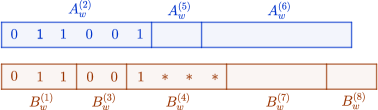
Figure 3: Here $\ast$ represents either $0$ or $1$. In the construction of the polynomial $\mathsf{ks}_{w}$, for $i=2$ and $\sigma=011001$, we have $f_{011001}^{(2)}=y_{011}^{(1)}\cdot y_{00}^{(3)}\cdot(y_{1000}^{(4)}+y_{1001}^{(4)}+\cdots+y_{1111}^{(4)})$.

The basic idea behind the above construction is simple. Given a monomial $m$ that is set-multilinear over $w|_{N_{w}}$, consider the partial assignment $\tau_{m}$ to the negative variables that sends any variable in $m$ to $1$ and all other negative variables to $0$. Now after applying $\tau_{m}$ to $\mathsf{ks}_{w}$ we are left with a simple subset sum instance

$$\sum_{i\in P_{w}}x_{\sigma_{i}}^{(i)}-\beta,$$

where $\sigma_{i}$ is the binary string indexed by $A_{w}^{(i)}$ that agrees with $\sigma(m)$ on $A_{w}^{(i)}$. Similarly for any monomial that is set-multilinear over $w|_{T}$ for some $T\subseteq N_{w}$, the polynomial $\tau_{m}(\mathsf{ks}_{w})$ is the subset sum instance

$$\sum_{i\in S}x_{\sigma_{i}}^{(i)}-\beta,$$

where $S$ is the maximal subset of $P_{w}$ such that $A_{w}^{S}\subseteq B_{w}^{T}$. With 5 we have a very good understanding of the multilinear IPS refutations of such subset sum instances, namely we know that the multilinear polynomial $f$ that equals

$$\frac{1}{\sum_{i\in S}x_{\sigma_{i}}^{(i)}-\beta}\text{ over Boolean assignments}$$

has as its leading monomials the product $\prod_{i\in S}x_{\sigma_{i}}^{(i)}$. This observation allows us to prove our rank lower bound in the following section. Figure 5 in subsection 3.2 illustrates the way assignments to the negative variables give rise to simple subset sum instances.

3.2 Rank Lower Bound Lemma

In this section we prove the main technical lemma of this paper – a rank lower bound for subset sum over any balanced word. Let $w\in\mathbb{Z}^{d}$ be any word, and let $f$ be a multilinear polynomial in the variables $\overline{X}(w)$. Denote by $M(f)$ the coefficient matrix of $f$ with rows indexed by all multilinear monomials (of any degree) in the positive variables and columns indexed by all multilinear monomials (again, of any degree) in the negative variables, and denote by $M_{w}(f)$ its submatrix with rows indexed by all monomials that are set-multilinear over $w|_{P_{w}}$ and columns indexed by all monomials that are set-multilinear over $w|_{N_{w}}$.

Figure 4: The coefficient matrix $M(f)$ with rows and columns indexed by the multilinear monomials over the $x$-variables and $y$-variables respectively; and its submatrix $M_{w}(f)$ with rows and columns indexed by the set-multilinear monomials over $w|_{P_{w}}$ and $w|_{N_{w}}$ respectively. If $w$ is a balanced word and $f$ is a multilinear polynomial agreeing with $\nicefrac{{1}}{{\mathsf{ks}_{w}}}$ over boolean assignments, then $M_{w}(f)$ has full-rank

Lemma 6.

Let $w\in\mathbb{Z}^{d}$ be a balanced word, and let $f$ be the multi-linear polynomial so that

$$f=\frac{1}{\mathsf{ks}_{w}}\text{ over Boolean assignments}.$$

Then $M_{w}(f)$ is full-rank.

Proof.

Without loss of generality we assume that $|w_{N_{w}}|\geq|w_{P_{w}}|$, so that our notation matches that of Section 3.1. Write

$$f=\sum_{m}g_{m}(x)m,$$ (3)

where the sum ranges over all multilinear monomials $m$ in the $y$-variables and $g_{m}(x)$ is some multilinear polynomial in the $x$-variables (note that here we include all multilinear monomials and not only the set-multilinear ones). We show that for any $m$ that is set-multilinear on $w|_{N_{w}}$ the leading monomial of $g_{m}(x)$ is the set-multilinear monomial $m(\sigma(m)|_{A_{w}^{P_{w}}})$. This is where we focus on the submatrix of set-multilinear monomials within the bigger matrix of all multilinear monomials, as depicted in Figure 4. To prove this we need the following claim.

Claim 7.

For any monomial $m$ set-multilinear on some $w|_{T}$, where $T\subseteq N_{w}$, the leading monomial of $g_{m}(x)$ is less or equal to

$$m\left(\sigma(m)|_{A_{w}^{S}}\right),$$

where $S$ is the maximal subset of $P_{w}$ such that $A_{w}^{S}\subseteq B_{w}^{T}$.

Moreover if $m$ is set-multilinear on $w|_{N_{w}}$, then the leading monomial of $g_{m}(x)$ equals

$$m\left(\sigma(m)|_{A_{w}^{P_{w}}}\right).$$

Proof of Claim..

Proof by induction on the size of $T$.

Base case: If $T=\emptyset$, the only monomial set-multilinear on $w|_{\emptyset}$ is the empty monomial $1$. Now consider the partial assignment $\tau_{1}$ that maps all the ${\overline{y}}$-variables to $0$. Now $\tau_{1}(f)=g_{1}(x)$, where $g_{1}(x)$ is the coefficient of the empty monomial $1$. On the other hand, since

$$f=\frac{1}{\mathsf{ks}_{w}}\text{\quad over Boolean assignments,}$$

we have that $\tau_{1}(f)=1/-\beta$ over Boolean assignments. As $g_{1}(x)$ is multilinear, $g_{1}(x)=1/-\beta$ as a polynomial identity and so the leading monomial of $g_{1}(x)$ is the empty monomial $1$.

Induction step: Suppose then that $T$ is non-empty, and let $m$ be a set-multilinear monomial on $w|_{T}$. Now consider the partial assignment $\tau_{m}$ that maps any variable in $m$ to $1$ and any other ${\overline{y}}$-variable to $0$. By Equation 3

$$\tau_{m}(f)=\sum_{m^{\prime}}g_{m^{\prime}}(x),$$ (4)

where $m^{\prime}$ ranges over all submonomials of $m$. On the other hand, by the construction of $\mathsf{ks}_{w}$

$$\tau_{m}(f)=\frac{1}{\sum x^{(i)}_{\sigma}-\beta}\text{\quad over Boolean assignments,}$$

where the sum in the denominator ranges over those $i$ and $\sigma$ such that $A_{w}^{(i)}\subseteq B_{w}^{T}$ and $\sigma$ agrees with $\sigma(m)$ on the interval $A_{w}^{(i)}$. Note that for any $i\in P_{w}$ there is at most one $\sigma$ such that $x^{(i)}_{\sigma}$ appears in the sum (because $A_{w}^{(i)}\subseteq B_{w}^{T}$, and by construction of $\mathsf{ks}_{w}$, $x_{\sigma}^{(i)}$ for a fixed $\sigma$ is multiplied in $\mathsf{ks}_{w}$ by all products $\Pi_{j}y^{(j)}_{\rho_{j}}$ such that the concatenation of the $\rho_{j}$’s extends the string $\sigma$; but since we assigned 0-1 to all the ${\overline{y}}$-variables there is a single such concatenation, induced by our assignment of 1’s; see Figure 3).

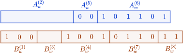
Figure 5: In this example, $T=\{1,4,7,8\}\subseteq N_{w}$ and $m=y_{100}^{(1)}\cdot y_{1001}^{(4)}\cdot y_{0110}^{(7)}\cdot y_{11}^{(8)}$ is a set-multilinear monomial over $w|_{T}$. As $S=\{5,6\}$ is the maximal subset of $P_{w}$ such that $A_{w}^{S}\subseteq B_{w}^{T}$, we therefore have that the leading monomial of $g_{m}(x)$ (from Equation 3) is less than or equal to $x_{00}^{(5)}\cdot x_{101101}^{(6)}$. Moreover, in the polynomial $\textbf{ks}_{w}$, the partial assignment setting the $y$-variables in $m$ to $1$ and the remaining $y$-variables to $0$ results in the polynomial $x_{00}^{(5)}+x_{101101}^{(6)}-\beta$.

It follows by 5 that the leading monomial of $\tau_{m}(f)$ is the product of all the $x^{(i)}_{\sigma}$ appearing in the sum in the denominator above, and thus the leading monomial equals

$$m\left(\sigma(m)|_{A_{w}^{S}}\right),$$ (5)

where $S$ is the maximal subset of $P_{w}$ such that $A_{w}^{S}\subseteq B_{w}^{T}$. By Equation 4, this means that either the leading monomial of $g_{m}(x)$ is less than or equal to (5), or otherwise is greater than (5) but is cancelled out in (4) by some monomial in $g_{m^{\prime}}(x)$ for $m^{\prime}$ a proper submonomial of $m$. But by induction assumption, for a proper submonomial $m^{\prime}$ of $m$ with $T^{\prime}\subsetneq T$ and $m^{\prime}$ set-multilinear on $w|_{T^{\prime}}$, the leading monomial of $g_{m^{\prime}}(x)$ is less or equal to $m\left(\sigma(m^{\prime})|_{A_{w}^{S^{\prime}}}\right)$, where $S^{\prime}$ is the maximal subset of $P_{w}$ such that $A_{w}^{S^{\prime}}\subseteq B_{w}^{T^{\prime}}$. Since, $m^{\prime}$ is a submonomial of $m$ the monomial $m\left(\sigma(m^{\prime})|_{A_{w}^{S^{\prime}}}\right)$ is less than or equal to $m\left(\sigma(m)|_{A_{w}^{S}}\right)$, and so the above mentioned cancellation cannot occur, and we conclude that the leading monomial of $g_{m}(x)$ is less than or equal to (5).

It remains to show that the leading monomial of $g_{m}(x)$ is precisely (5), when $m$ is a set-multilinear monomial on $w|_{N_{w}}$. Let $m^{\prime}$ be a proper submonomial of $m$ that is set-multilinear over $w|_{T}$ for some $T\subsetneq N_{w}$. By the assumption that $w$ is balanced there is some $i\in P_{w}$ such that $A_{w}^{(i)}\nsubseteq B_{w}^{T}$, and thus the leading monomial of $g_{m^{\prime}}(x)$ is properly smaller than $m(\sigma(m)|_{A_{w}^{P_{w}}})$. Hence, by Equation 5 (and the sentence preceding it) the leading monomial of $g_{m}(x)$ must equal $m(\sigma(m)|_{A_{w}^{P_{w}}})$. ∎

By the claim for any $m$ that is set-multilinear on $w|_{N_{w}}$ the leading monomial of $g_{m}(x)$ is the monomial $m(\sigma(m)|_{A_{w}^{P_{w}}})$, and these include all the set-multilinear monomials on $w|_{P_{w}}$. Thus the column space of $M_{w}(f)$ spans the space of all set-multilinear polynomials on $w|_{P_{w}}$, and $M_{w}(f)$ is full-rank (where a column in $M_{w}(f)$ determines a polynomial that is a linear combination of the positive monomials in its rows).

∎

Corollary 8.

Let $w\in\mathbb{Z}^{d}$ be a balanced word with $|w_{i}|\leq b$ for all $i\in[d]$, and let $f$ be the multi-linear polynomial so that

$$f=\frac{1}{\mathsf{ks}_{w}}\text{ over Boolean assignments}.$$

Then $\mathrm{relrk}_{w}(f)\geq 2^{-b/2}$.

Proof.

Assume again without a loss of generality that $|w_{N_{w}}|\geq|w_{P_{w}}|$. By the “balanced-ness” and the assumption that $|w_{i}|\leq b$ for all $i\in[d]$, we know that $|w_{P_{w}}|-|w_{N_{w}}|\geq-b$. By 6, $M_{w}(f)$ is of rank $|M^{P}_{w}|$, and so

$$\mathrm{relrk}_{w}(f)=\sqrt{\frac{|M^{P}_{w}|}{|M^{N}_{w}|}}=\sqrt{2^{|w_{P_{w}}|-|w_{N_{w}}|}}\geq 2^{-b/2}.$$

∎

3.3 Lower Bound for Constant-Depth Set-Multilinear Circuits

In this section we prove the following lower bound on bounded-depth set-multilinear circuits.

Lemma 9.

Let $d,k,\Delta\in\mathbb{N}_{+}$ with $k\geq 10d$. Let $w\in\mathbb{Z}^{d}$ be a balanced word in the vocabulary $\{\lfloor\alpha k\rfloor,-k\}$, where $\alpha=\nicefrac{{1}}{{\sqrt{2}}}$, and let $f$ be the multilinear polynomial which equals $\nicefrac{{1}}{{\mathsf{ks}_{w}}}$ over Boolean assignments. Then any set-multilinear circuit of product-depth $\Delta$ computing the set-multilinear projection $\Pi_{w}(f)$ has size at least

$$2^{k\left(\frac{d^{\nicefrac{{1}}{{(2^{\Delta}-1)}}}-20}{40\Delta}\right)}$$

Proof.

We prove the lemma by using the following claim from [17].

Claim 10 ([17] Claim 16).

Let $k\geq 10d$. Let $w$ be any word of length $d$ with entries in $\{\lfloor\alpha k\rfloor,-k\}$, where $\alpha=\nicefrac{{1}}{{\sqrt{2}}}$. Then for any $\Delta\geq 1$, any set-multilinear formula $C$ of product-depth $\Delta$ of size at most $s$ satisfies

$$\mathrm{relrk}_{w}(C)\leq s\,\cdot\,2^{\frac{-kd^{\nicefrac{{1}}{{(2^{\Delta}-1)}}}}{20}}$$

Let $C$ be a set-multilinear circuit of size $s$ and product-depth $\Delta$ computing $\Pi_{w}(f)$. We can transform $C$ into a set-multilinear formula $F$ of size $s^{2\Delta}$ and product-depth $\Delta$ computing $\Pi_{w}(f)$.

Now by 6 and 10, we have that

$$2^{-k}\leq\mathrm{relrk}_{w}(\Pi_{w}(f))\leq s^{2\Delta}\,\cdot\,2^{\frac{-kd^{\nicefrac{{1}}{{(2^{\Delta}-1)}}}}{20}},$$

and thus

$$s^{2\Delta}\geq 2^{k\left(\frac{d^{\nicefrac{{1}}{{(2^{\Delta}-1)}}}-20}{20}\right)},$$

from which the claim follows. ∎

3.4 Lower Bound for Constant-Depth Circuits

Finally in this section we prove Theorem 4. To prove this theorem we reduce the task of computing $f$ in Theorem 4 to computing the set-multilinear projection $\Pi_{w}(f^{\prime})$ of the multilinear $f^{\prime}$ that equals $\nicefrac{{1}}{{\mathsf{ks}_{w}}}$ over the Boolean values for a suitable word $w$. For this we require the following lemma which can be proved in a manner similar to Proposition 9 in [17].

Lemma 11.

Let $s,N,d$ and $\Delta$ be growing parameters with $s\geq Nd$. Assume that $\operatorname{char}(\mathbb{F})=0$ or $\operatorname{char}(\mathbb{F})>d$. Let $C$ be a circuit of size at most $s$ and product-depth at most $\Delta$ computing a polynomial $f$. Let $\overline{X}=\langle X_{1},\ldots,X_{d}\rangle$ be a sequence of pairwise disjoint sets of variables, each of size at most $N$. Then there is a set-multilinear circuit $\tilde{C}$ of size at most $d^{O(d)}{\mathsf{poly}}(s)$ and product-depth at most $2\Delta$ computing the set-multilinear projection $\Pi_{\overline{X}}(f)$ of $f$.

With this lemma at hand, we are ready to prove Theorem 4.

Proof of Theorem 4.

Let $C$ be a circuit of size at most $s\geq n$ and product-depth $\Delta$ computing $f$. Now let $k=\lfloor\nicefrac{{\log n}}{{2}}\rfloor$ and $d=\lfloor\nicefrac{{\log n}}{{25}}\rfloor$, and note that $d2^{k}<n\leq s$ for large enough $n$. Note also that $k\geq 10d$ for large enough $n$. Let $w$ be a balanced word of length $d$ on the alphabet $\{\lfloor\alpha k\rfloor,-k\}$. One can easily construct such a word by induction on $d$.

Note that the polynomial $\mathsf{ks}_{w}$ is now of degree at most $4$, as any $B_{w}^{(j)}$ overlaps at most $3$ different $A_{w}^{(i)}$’s and any $A_{w}^{(i)}$ overlaps at most $2$ different $B_{w}^{(j)}$’s. Also, by choice of parameters, $\mathsf{ks}_{w}$ involves less than $n$ many variables. Hence there is some partial assignment $\tau_{w}$ to the variables $\{z_{ijk\ell},x_{i}:i,j,k,\ell\in[n]\}$ that maps $\sum_{i,j,k,\ell\in[n]}z_{ijk\ell}x_{i}x_{j}x_{k}x_{\ell}-\beta$ to the polynomial $\mathsf{ks}_{w}$ (up to renaming of variables). By applying this partial mapping to $C$, we obtain a circuit $C^{\prime}$ of size at most $s$ and product-depth $\Delta$ that computes the multilinear $f^{\prime}$ that equals $\nicefrac{{1}}{{\mathsf{ks}_{w}}}$ over Boolean assignments. Now, by Lemma 11, there is a set-multilinear circuit $C^{\prime}$ of size $d^{O(d)}{\mathsf{poly}}(s)$ and product-depth $2\Delta$ computing the set-multilinear projection $\Pi_{w}(f^{\prime})$ of $f^{\prime}$.

By 9 any set-multilinear circuit of product-depth $2\Delta$ computing $\Pi_{w}(f^{\prime})$ has size at least

$$2^{k\left(\frac{d^{\nicefrac{{1}}{{(2^{2\Delta}-1)}}}-20}{80\Delta}\right)}\geq n^{\frac{d^{\nicefrac{{1}}{{(2^{2\Delta}-1)}}}-20}{200\Delta}}.$$

Putting everything together we have that

$$d^{O(d)}{\mathsf{poly}}(s)\geq n^{\frac{d^{\nicefrac{{1}}{{(2^{2\Delta}-1)}}}-20}{200\Delta}}.$$

Now, given that $\Delta\leq\nicefrac{{1}}{{4}}\log\log\log n$, by the choice of $d$, we have that $2\Delta\leq\nicefrac{{1}}{{2}}\log\log 30d$. Then for large enough $n$ we have that

$$n^{\frac{d^{\nicefrac{{1}}{{(2^{2\Delta}-1)}}}-20}{200\Delta}}\geq n^{\frac{2^{\sqrt{\log(d/30)}/2}}{50\log\log 30d}},$$

and as

$$n^{\frac{2^{\sqrt{\log(d/30)}/2}}{50\log\log 30d}}\geq d^{\omega(d)},$$

the lower bound follows.

∎

Comment: We remark that if we make sure that the word $w$ above leans towards the negative monomials, meaning that $|w_{N_{w}}|\geq|w_{P_{w}}|$, we can actually prove the lower bound for the following degree-$4$ variant of subset-sum

$$\sum_{i,j,k\in[n]}z_{ijk}x_{i}x_{j}x_{k}-\beta.$$

We have however opted for the proof above for simplicity, as it works for any balanced word over the vocabulary $\{\lfloor\alpha k\rfloor,-k\}$ and does not involve any set-up of a suitable word that could distract from the main idea.

4 Conclusions and Open Problems

The main goal of this work is to advance on the frontiers of strong propositional proofs lower bounds. We provide the first lower bounds against algebraic proof systems operating with constant-depth circuits, where the hard instance is computable itself with small constant-depth circuits. Our hard instances are combinatorial, simple, and have 0-1 coefficients, and the lower bounds work in the unit-cost model of algebraic circuits, namely, where the size does not depend on the magnitude of coefficients used in the polynomials appearing in the proof

Thus, our result brings us to the natural and standard setting of proof complexity lower bounds, while coming closer to CNF hard instances (since the magnitude of coefficients in the hard instances do not play a role in our lower bound proofs).

On the other hand, establishing lower bounds against CNF formulas in strong algebraic proof systems stays a remarkable open problem, since it necessitates a lower bound technique that is different from the functional lower bound approach we used or the bit-complexity/large-coefficients approach of [1, 2] (or at least a substantially modified technique than those two techniques). Note that such lower bounds would also imply constant-depth Frege with counting gates (${\rm AC}^{0}[p]$-Frege) lower bounds, which is an important long-standing open problem in proof complexity. This leads us to the following set of open problems:

1. CNF hard instances: Can we establish lower bounds against strong algebraic proof systems, and specifically constant-depth IPS proofs for a family of CNF formulas? As mentioned above, this is a very challenging problem, or at least one with important consequences in proof complexity.

Before tackling this difficult open problem, we identify several possibly less challenging ones that seem to be prerequisites for solving open problem 1 (at least as far as taking the proof complexity lower bound approach in the current paper):

1. Finite fields: Can we establish lower bounds against strong algebraic proof systems, and specifically constant-depth IPS proofs over finite fields? Both the functional lower bound argument from Forbes et al. [8] and the Limaye et al. [17] technique, use the fact that the fields are sufficiently big, or have characteristic 0. For the former approach, characteristic 0 fields are essential: first, the subset sum instance is not necessarily unsatisfiable over finite fields. But more crucially, the whole functional lower bound approach for IPS hinges on lower bounding the size of a circuit computing the function $\nicefrac{{1}}{{f}}$ over the Boolean cube, for some efficiently computable polynomial $f$. However, over finite fields $\nicefrac{{1}}{{f}}$ is efficiently computed, when $f$ is, over the Boolean cube. For the latter [17] approach, large fields do not seem to be as crucial to the argument (it is used only in the homogenization procedure to yield low-depth circuits, using polynomial interpolation, the latter requires a sufficiently large field; this homogenization is based on a generalization of Shpilka and Wigderson [25]). However, there may be a different way to homogenize constant-depth circuits without increasing too much the depth even over finite fields.

2. No multilinear requirement: Can we get rid of the requirement for multilinearity of the IPS refutations in our lower bounds? Namely, can we use a stronger proof system than multilinear $\textup{IPS}_{\text{LIN}^{\prime}}$? We discussed this requirement in the introduction. It comes from the requirement in the Limaye et al. [17] technique to consider set-multilinear polynomials, as well as the use of the functional lower bound approach from [8] which focuses on functions computed on the Boolean cube alone. A hard set-multilinear polynomial can compute the same function over the Boolean cube as a polynomial whose set-multilinear projection is in fact zero (and hence easy to compute), which breaks our argument. It is unclear at the moment how to overcome this obstacle. This leads us to the following interesting question in algebraic circuit complexity proper:

3. Functional lower bounds for constant-depth circuits: Can we prove a lower bound on the size of every constant-depth circuit computing a certain function (in contrast to a certain specific polynomial; this is the difference between “semantic” lower bounds, and the weaker notion of “syntactic” lower bounds in algebraic circuit complexity)?

References

- [1] Yaroslav Alekseev. A lower bound for polynomial calculus with extension rule. In Valentine Kabanets, editor, 36th Computational Complexity Conference, CCC 2021, July 20-23, 2021, Toronto, Ontario, Canada (Virtual Conference), volume 200 of LIPIcs, pages 21:1–21:18. Schloss Dagstuhl - Leibniz-Zentrum für Informatik, 2021.
- [2] Yaroslav Alekseev, Dima Grigoriev, Edward A. Hirsch, and Iddo Tzameret. Semi-algebraic proofs, IPS lower bounds, and the -conjecture: can a natural number be negative? In Proceedings of the 52nd Annual ACM SIGACT Symposium on Theory of Computing, STOC 2020, pages 54–67. ACM, 2020.
- [3] Robert Andrews and Michael A. Forbes. Ideals, determinants, and straightening: Proving and using lower bounds for polynomial ideals. In 54th Annual ACM SIGACT Symposium on Theory of Computing, STOC 2022, 2022.
- [4] Paul Beame, Russell Impagliazzo, Jan Krajíček, Toniann Pitassi, and Pavel Pudlák. Lower bounds on Hilbert’s Nullstellensatz and propositional proofs. Proc. London Math. Soc. (3), 73(1):1–26, 1996.
- [5] Samuel R. Buss, Russell Impagliazzo, Jan Krajíček, Pavel Pudlák, Alexander A. Razborov, and Jiří Sgall. Proof complexity in algebraic systems and bounded depth Frege systems with modular counting. Computational Complexity, 6(3):256–298, 1996.
- [6] Matthew Clegg, Jeffery Edmonds, and Russell Impagliazzo. Using the Groebner basis algorithm to find proofs of unsatisfiability. In Proceedings of the 28th Annual ACM Symposium on the Theory of Computing (Philadelphia, PA, 1996), pages 174–183, New York, 1996. ACM.
- [7] David Cox, John Little, and Donal O’Shea. Ideals, varieties, and algorithms. Undergraduate Texts in Mathematics. Springer, New York, third edition, 2007. An introduction to computational algebraic geometry and commutative algebra.
- [8] Michael A. Forbes, Amir Shpilka, Iddo Tzameret, and Avi Wigderson. Proof complexity lower bounds from algebraic circuit complexity. Theory Comput., 17:1–88, 2021.
- [9] Mika Göös and Toniann Pitassi. Communication lower bounds via critical block sensitivity. SIAM J. Comput., 47(5):1778–1806, 2018.
- [10] Dima Grigoriev and Edward A. Hirsch. Algebraic proof systems over formulas. Theoret. Comput. Sci., 303(1):83–102, 2003. Logic and complexity in computer science (Créteil, 2001).
- [11] Joshua A. Grochow and Toniann Pitassi. Circuit complexity, proof complexity, and polynomial identity testing: The ideal proof system. J. ACM, 65(6):37:1–37:59, 2018.
- [12] Russell Impagliazzo, Sasank Mouli, and Toniann Pitassi. The surprising power of constant depth algebraic proofs. In Holger Hermanns, Lijun Zhang, Naoki Kobayashi, and Dale Miller, editors, LICS ’20: 35th Annual ACM/IEEE Symposium on Logic in Computer Science, Saarbrücken, Germany, July 8-11, 2020, pages 591–603. ACM, 2020.
- [13] Russell Impagliazzo, Sasank Mouli, and Toniann Pitassi. Lower bounds for polynomial calculus with extension variables over finite fields. Electron. Colloquium Comput. Complex., 2022.
- [14] Russell Impagliazzo, Pavel Pudlák, and Jiří Sgall. Lower bounds for the polynomial calculus and the Gröbner basis algorithm. Computational Complexity, 8(2):127–144, 1999.
- [15] Alexander Knop. Ips-like proof systems based on binary decision diagrams. Electron. Colloquium Comput. Complex., page 179, 2017.
- [16] Fu Li, Iddo Tzameret, and Zhengyu Wang. Characterizing propositional proofs as noncommutative formulas. In SIAM Journal on Computing, volume 47, pages 1424–1462, 2018. Full Version: http://arxiv.org/abs/1412.8746.
- [17] Nutan Limaye, Srikanth Srinivasan, and Sébastien Tavenas. Superpolynomial lower bounds against low-depth algebraic circuits. In 62nd IEEE Annual Symposium on Foundations of Computer Science, FOCS 2021, Denver, CO, USA, February 7-10, 2022, pages 804–814. IEEE, 2021.
- [18] Toniann Pitassi. Algebraic propositional proof systems. In Descriptive complexity and finite models (Princeton, NJ, 1996), volume 31 of DIMACS Ser. Discrete Math. Theoret. Comput. Sci., pages 215–244. Amer. Math. Soc., Providence, RI, 1997.
- [19] Toniann Pitassi. Unsolvable systems of equations and proof complexity. In Proceedings of the International Congress of Mathematicians, Vol. III (Berlin, 1998), number Vol. III, pages 451–460, 1998.
- [20] Tonnian Pitassi and Iddo Tzameret. Algebraic proof complexity: Progress, frontiers and challenges. ACM SIGLOG News, 3(3), 2016.
- [21] Ran Raz and Iddo Tzameret. Resolution over linear equations and multilinear proofs. Ann. Pure Appl. Logic, 155(3):194–224, 2008.
- [22] Ran Raz and Iddo Tzameret. The strength of multilinear proofs. Computational Complexity, 17(3):407–457, 2008.
- [23] Alexander A. Razborov. Lower bounds for the polynomial calculus. Comput. Complexity, 7(4):291–324, 1998.
- [24] Ramprasad Saptharishi. A survey of lower bounds in arithmetic circuit complexity, 2016-2022. https://github.com/dasarpmar/lowerbounds-survey/releases.
- [25] Amir Shpilka and Avi Wigderson. Depth-3 arithmetic circuits over fields of characteristic zero. Comput. Complexity, 10:1–27, 2001.
- [26] Amir Shpilka and Amir Yehudayoff. Arithmetic circuits: A survey of recent results and open questions. Foundations and Trends in Theoretical Computer Science, 5(3-4):207–388, 2010.
- [27] Iddo Tzameret. Algebraic proofs over noncommutative formulas. Inf. Comput., 209(10):1269–1292, 2011.