Minimal-Perimeter Lattice Animals and the Constant-Isomer Conjecture

Abstract

We consider minimal-perimeter lattice animals, providing a set of conditions which are sufficient for a lattice to have the property that inflating all minimal-perimeter animals of a certain size yields (without repetitions) all minimal-perimeter animals of a new, larger size. We demonstrate this result on the two-dimensional square and hexagonal lattices. In addition, we characterize the sizes of minimal-perimeter animals on these lattices that are not created by inflating members of another set of minimal-perimeter animals.

1 Introduction

An animal on a $d$-dimensional lattice is a connected set of lattice cells, where connectivity is through ($d{-}1$)-dimensional faces of the cells. Specifically, on the planar square lattice, connectivity of cells is through edges. Two animals are considered identical if one can be obtained from the other by translation only, without rotations or flipping. (Such animals are called “fixed” animals, as opposed to “free” animals.)

Lattice animals attracted interest in the literature as combinatorial objects [9] and as a computational model in statistical physics and chemistry [16]. (In these areas, one usually considers site animals, that is, clusters of lattice vertices, hence, the graphs considered there are the dual of our graphs.) In this paper, we consider lattices in two dimensions, specifically, the hexagonal, triangular, and square lattices, where animals are called polyhexes, polyiamonds, and polyominoes, respectively. We show the application of our results to the square and hexagonal lattices, and explain how to extend the latter to the triangular lattice. An example of such animals is shown in figure 1.

Figure 1: An example of a polyomino, a polyhex, and a polyiamond.

Let $A^{\mathcal{L}}(n)$ denote the number of lattice animals of size $n$, that is, animals composed of $n$ cells, on a lattice $\mathcal{L}$. A major research problem in the study of lattices is understanding the nature of $A^{\mathcal{L}}(n)$, either by finding a formula for it as a function of $n$, or by evaluating it for specific values of $n$. These problems are to this date still open for any nontrivial lattice. Redelmeier [14] introduced the first algorithm for counting all polyominoes of a given size, with no polyomino being generated more than once. Later, Mertens [13] showed that Redelmeier’s algorithm can be utilized for any lattice. The first algorithm for counting lattice animals without generating all of them was introduced by Jensen [12]. Using his method, the number of animals on the 2-dimensional square, hexagonal, and triangular lattices were computed up to size 56, 46, and 75, respectively.

An important measure of lattice animals is the size of their perimeter (sometimes called “site perimeter”). The perimeter of a lattice animal is defined as the set of empty cells adjacent to the animal cells. This definition is motivated by percolation models in statistical physics. In such discrete models, the plane or space is made of small cells (squares or cubes, respectively), and quanta of material or energy “jump” from a cell to a neighboring cell with some probability. Thus, the perimeter of a cluster determines where units of material or energy can move to, and guide the statistical model of the flow.

(a) Q

(b) I(Q)

Figure 2: A polyomino $Q$ and its inflated polyomino $I(Q)$. Polyomino cells are colored gray, while perimeter cells are colored white.

Asinowski et al. [2, 3] provided formulae for polyominoes and polycubes with perimeter size close to the maximum possible. On the other extreme reside animals with the minimum possible perimeter size for their area. The study of polyominoes of a minimal perimeter dates back to Wang and Wang [18], who identified an infinite sequence of cells on the square lattice, the first $n$ of which (for any $n$) form a minimal-perimeter polyomino. Later, Altshuler et al. [1], and independently Sieben [15], studied the closely-related problem of the maximum area of a polyomino with $p$ perimeter cells, and provided a closed formula for the minimum possible perimeter of $n$-cell polyominoes.

Minimal-perimeter animals were also studied on other lattices. For animals on the triangular lattice (polyiamonds), the main result is due to Fülep and Sieben [10], who characterized all the polyiamonds with maximum area for their perimeter, and provided a formula for the minimum perimeter of a polyiamond of size $n$. Similar results were given by Vainsencher and Bruckstein [17] for the hexagonal lattice. In this paper, we study an interesting property of minimal-perimeter animals, which relates to the notion of the inflation operation. Simply put, inflating an animal is adding to it all its perimeter cells (see Figure 2). We provide a set of conditions (for a given lattice), which if it holds , then inflating all minimal-perimeter animals of some size yields all minimal-perimeter animals of some larger size in a bijective manner.

While this paper discusses some combinatorial properties of minimal-perimeter polyominoes, another algorithmic question emerges from these properties, namely, “how many minimal-perimeter polyominoes are there of a given size?” This question is addressed in detail in a companion paper [4].

The paper is organized as follows. In Section 2, we provide some definitions and prove our main theorem. In sections 3 and 4, we show the application of Section 2 to polyominoes and polyhexes, respectivally. Then, in Section 5 we explain how the same result also applies to the regular triangular lattice. We end in Section 6 with some concluding remarks.

1.1 Polyhexes as Molecules

In addition to research of minimal-perimeter animals in the literature on combinatorics, there has been much more intensive research of minimal-perimeter polyhexes in the literature on organic chemistry, in the context of the structure of families of molecules. For example, significant amount of work dealt with molecules called benzenoid hydrocarbons. It is a known natural fact that molecules made of carbon atoms are structured as shapes on the hexagonal lattice. Benzenoid hydrocarbons are made of carbon and hydrogen atoms only. In such a molecule, the carbon atoms are arranged as a polyhex, and the hydrogen atoms are arranged around the carbons atoms.

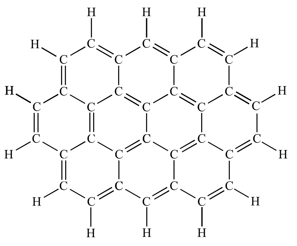
(a) Naphthalene ($C_{10}H_{8}$)		(b) Circumnaphtaline ($C_{32}H_{14})$

Figure 3: Naphthalene and its circumscribed version.

Figure 3(a) shows a schematic drawing of the molecule of Naphthalene (with formula $C_{10}H_{8}$), the simplest benzenoid hydrocarbon, which is made of ten carbon atoms and eight hydrogen atoms, while Figure 3(b) shows Circumnaphthalene (molecular formula $C_{32}H_{14}$). There exist different configurations of atoms for the same molecular formula, which are called isomers of the same formula. In the field of organic chemistry, a major goal is to enumerate all the different isomers of a given formula. Note that the carbon and hydrogen atoms are modeled by lattice vertices and not by cells of the lattice, but as we explain below, the numbers of hydrogen atoms identifies with the number of perimeter cells of the polyhexes under discussion. Indeed, the hydrogen atoms lie on lattice vertices that do not belong to the polyhex formed by the carbon atoms (which also lie on lattice vertices), but are connected to them by lattice edges. In minimal-perimeter polyhexes, each perimeter cell contains exactly two such hydrogen vertices, and every hydrogen vertex is shared by exactly two perimeter cells. (This has nothing to do with the fact that a single cell of the polyhex might be neighboring several—five, in the case of Naphthalene—“empty” cells.) Therefore, the number of hydrogen atoms in a molecule of a benzenoid hydrocarbon is identical to the size of the perimeter of the imaginary polyhex.

In a series of papers (culminated in Reference [7]), Dias provided the basic theory for the enumeration of benzenoid hydrocarbons. A comprehensive review of the subject was given by Brubvoll and Cyvin [5]. Several other works [11, 6, 8] also dealt with the properties and enumeration of such isomers. The analogue of what we call the “inflation” operation is called circumscribing in the literature on chemistry. A circumscribed version of a benzenoid hydrocarbon molecule $M$ is created by adding to $M$ an outer layer of hexagonal “carbon cells,” that is, not only the hydrogen atoms (of $M$) adjacent to the carbon atoms now turn into carbon atoms, but also new carbon atoms are added at all other “free” vertices of these cells so as to “close” them. In addition, hydrogen atoms are put at all free lattice vertices that are connected by edges to the new carbon atoms. This process is visualized well in Figure 3. In the literature on chemistry, it is well known that circumscribing all isomers of a given molecular formula yields, in a bijective manner, all isomers that correspond to another molecular formula. (The sequences of molecular formulae that have the same number of isomers created by circumscribing are known as constant-isomer series.) Although this fact is well known, to the best of our knowledge, no rigorous proof of it was ever given.

As mentioned above, we show that inflation induces a bijection between sets of minimal-perimeter animals on the square, hexagonal, and in a sense, also on the triangular lattice. By this, we prove the long-observed (but never proven) phenomenon of “constant-isomer series,” that is, that circumscribing isomers of benzenoid hydrocarbon molecules (in our terminology, inflating minimum-perimeter polyhexes) yields all the isomers of a larger molecule.

2 Minimal-Perimeter Animals

Throughout this section, we consider animals on some specific lattice $\mathcal{L}$. Our main result consists of a set of conditions on minimal-perimeter animals on $\mathcal{L}$, which is sufficient for satisfying a bijection between sets of minimal-perimeter animals on $\mathcal{L}$.

2.1 Preliminaries

$Q$		$I(Q)$		$D(Q)$

Figure 4: A polyhex $Q$, its inflated polyhex $I(Q)$, and its deflated polyhex $D(Q)$. The gray cells belong to $Q$, the white cells are its perimeter, and its border cells are marked with a pattern of dots.

Let $Q$ be an animal on $\mathcal{L}$. Recall that the perimeter of $Q$, denoted by $\mathcal{P}(Q)$, is the set of all empty lattice cells that are neighbors of at least one cell of $Q$. Similarly, the border of $Q$, denoted by $\mathcal{B}(Q)$, is the set of cells of $Q$ that are neighbors of at least one empty cell. The inflated version of $Q$ is defined as $I(Q):=Q\cup\mathcal{P}(Q)$. Similarly, the deflated version of $Q$ is defined as $D(Q):=Q\backslash\mathcal{B}(Q)$. These operations are demonstrated in Figure 4.

Denote by $\epsilon(n)$ the minimum possible size of the perimeter of an $n$-cell animal on $\mathcal{L}$, and by $M_{n}$ the set of all minimal-perimeter $n$-cell animals on $\mathcal{L}$.

2.2 A Bijection

Theorem 1

Consider the following set of conditions.

1. The function $\epsilon(n)$ is weakly-monotone increasing.

2. There exists some constant $c^{*}=c^{*}(\mathcal{L})$, for which, for any minimal-perimeter animal $Q$, we have that $\left|\mathcal{P}(Q)\right|=\left|\mathcal{B}(Q)\right|+c^{*}$ and $\left|\mathcal{P}(I(Q))\right|\leq\left|\mathcal{P}(Q)\right|+c^{*}$.

3. If $Q$ is a minimal-perimeter animal of size $n+\epsilon(n)$, then $D(Q)$ is a valid (connected) animal.

If all the above conditions hold for $\mathcal{L}$, then $\left|M_{n}\right|=\left|M_{n+\epsilon(n)}\right|$. If these conditions are not satisfied for only a finite amount of sizes of animals, then the claim holds for all sizes greater than some lattice-dependent nominal size $n_{0}$.

Proof:  We begin with proving that inflation preserves perimeter minimality.

Lemma 2

If $Q$ is a minimal-perimeter animal, then $I(Q)$ is a minimal-perimeter animal as well.

Proof:  Let $Q$ be a minimal-perimeter animal. Assume to the contrary that $I(Q)$ is not a minimal-perimeter animal, thus, there exists an animal $Q^{\prime}$ such that $\left|Q^{\prime}\right|=\left|I(Q)\right|$, and $\left|\mathcal{P}(Q^{\prime})\right|<\left|\mathcal{P}(I(Q))\right|$. By the second premise of Theorem 1, we know that $\left|\mathcal{P}(I(Q))\right|\leq\left|\mathcal{P}(Q)\right|+c^{*}$, thus, $\left|\mathcal{P}(Q^{\prime})\right|<\left|\mathcal{P}(Q)\right|+c$, and since $Q^{\prime}$ is a minimal-perimeter animal, we also know by the same premise that $\left|\mathcal{P}(Q^{\prime})\right|=\left|\mathcal{B}(Q^{\prime})\right|+c$, and, hence, that $\left|\mathcal{B}(Q^{\prime})\right|<\left|\mathcal{P}(Q)\right|$. Consider now the animal $D(Q^{\prime})$. Recall that $\left|Q^{\prime}\right|=\left|I(Q)\right|=\left|Q\right|+\left|\mathcal{P}(Q)\right|$, thus, the size of $D(Q^{\prime})$ is at least $\left|Q\right|+1$, and $\left|\mathcal{P}(D(Q^{\prime}))\right|<\left|\mathcal{P}(Q)\right|=\epsilon(n)$ (since the perimeter of $D(Q^{\prime})$ is a subset of the border of $Q^{\prime}$). This is a contradiction to the first premise, which states that the sequence $\epsilon(n)$ is monotone increasing. Hence, the animal $Q^{\prime}$ cannot exist, and $I(Q)$ is a minimal-perimeter animal. $\Box$

We now proceed to demonstrating the effect of repeated inflation on the size of minimal-perimeter animals.

Lemma 3

The minimum perimeter size of animals of size $n+k\epsilon(n)+c^{*}k(k-1)/2$ (for $n>1$ and any $k\in\mathbb{N}$) is $\epsilon(n)+c^{*}k$.

Proof:  We repeatedly inflate a minimal-perimeter animal $Q$, whose initial size is $n$. The size of the perimeter of $Q$ is $\epsilon(n)$, thus, inflating it creates a new animal of size $n+\epsilon(n)$, and the size of the border of $I(Q)$ is $\epsilon(n)$, thus, the size of $I(Q)$ is $\epsilon(n)+c^{*}$. Continuing the inflation of the animal, the $k$th inflation will increase the size of the animal by $\epsilon(n)+(k-1)c^{*}$ and will increase the size of the perimeter by $c^{*}$. Summing up these quantities yields the claim. $\Box$

Next, we prove that inflation preserves difference, that is, inflating two different minimal-perimeter animals (of equal or different sizes) always produces two different new animals. (Note that this is not true for non-minimal-perimeter animals.)

Lemma 4

Let $Q_{1},Q_{2}$ be two different minimal-perimeter animals. Then, regardless of whether or not $Q_{1},Q_{2}$ have the same size, the animals $I(Q_{1})$ and $I(Q_{2})$ are different as well.

Proof:  Assume to the contrary that $Q=I(Q_{1})=I(Q_{2})$, that is, $Q=Q_{1}\cup\mathcal{P}(Q_{1})=Q_{2}\cup\mathcal{P}(Q_{2})$. In addition, since $Q_{1}\neq Q_{2}$, and since a cell cannot belong simultaneously to both an animal and to its perimeter, this means that $\mathcal{P}(Q_{1})\neq\mathcal{P}(Q_{2})$. The border of $Q$ is a subset of both $\mathcal{P}(Q_{1})$ and $\mathcal{P}(Q_{2})$, that is, $\mathcal{B}(Q)\subset\mathcal{P}(Q_{1})\cap\mathcal{P}(Q_{2})$. Since $\mathcal{P}(Q_{1})\neq\mathcal{P}(Q_{2})$, we obtain that either $\left|\mathcal{B}(Q)\right|<\left|\mathcal{P}(Q_{1})\right|$ or $\left|\mathcal{B}(Q)\right|<\left|\mathcal{P}(Q_{2})\right|$; assume without loss of generality the former case. Now consider the animal $D(Q)$. Its size is $\left|Q\right|-\left|\mathcal{B}(Q)\right|$. The size of $Q$ is $\left|Q_{1}\right|+\left|\mathcal{P}(Q_{1})\right|$, thus, $\left|D(Q)\right|>\left|Q_{1}\right|$, and since the perimeter of $D(Q)$ is a subset of the border of $Q$, we conclude that $\left|\mathcal{P}(D(Q))\right|<\left|\mathcal{P}(Q_{1})\right|$. However, $Q_{1}$ is a minimal-perimeter animal, which is a contradiction to the first premise of the theorem, which states that $\epsilon(n)$ is monotone increasing. $\Box$

To complete the cycle, we also prove that for any minimal-perimeter animal $Q\in M_{n+\epsilon(n)}$, there is a minimal-perimeter source in $M_{n}$, that is, an animal $Q^{\prime}$ whose inflation yields $Q$. Specifically, this animal is $D(Q)$.

Lemma 5

For any $Q\in M_{n+\epsilon(n)}$, we also have that $I(D(Q))=Q$.

Proof:  Since $Q\in M_{n+\epsilon(n)}$, we have by Lemma 3 that $\left|\mathcal{P}(Q)\right|=\epsilon(n)+c^{*}$. Combining this with the equality $\left|\mathcal{P}(Q)\right|=\left|\mathcal{B}(Q)\right|+c^{*}$, we obtain that $\left|\mathcal{B}(Q)\right|=\epsilon(n)$, thus, $\left|D(Q)\right|=n$ and $\left|\mathcal{P}(D(Q))\right|\geq\epsilon(n)$. Since the perimeter of $D(Q)$ is a subset of the border of $Q$, and $\left|\mathcal{B}(Q)\right|=\epsilon(n)$, we conclude that the perimeter of $D(Q)$ and the border of $Q$ are the same set of cells, and, hence, $I(D(Q))=Q$. $\Box$

Let us now wrap up the proof of the main theorem. In Lemma 2 we have shown that for any minimal-perimeter animal $Q\in M_{n}$, we have that $I(Q)\in M_{n+\epsilon(n)}$. In addition, Lemma 4 states that the inflation of two different minimal-perimeter animals results in two other different minimal-perimeter animals. Combining the two lemmata, we obtain that $\left|M_{n}\right|\leq\left|M_{n+\epsilon(n)}\right|$. On the other hand, in Lemma 5 we have shown that if $Q\in M_{n+\epsilon(n)}$, then $I(D(Q))=Q$, and, thus, for any animal in $M_{n+\epsilon(n)}$, there is a unique source in $M_{n}$ (specifically, $D(Q)$), whose inflation yields $Q$. Hence, $\left|M_{n}\right|\geq\left|M_{n+\epsilon(n)}\right|$. Combining the two relations, we conclude that $\left|M_{n}\right|=\left|M_{n+\epsilon(n)}\right|$. $\Box$

2.3 Inflation Chains

Theorem 1 implies that there exist infinite chains of sets of minimal-perimeter animals, each set obtained by inflating all members of the previous set, while the cardinalities of all sets in a chain are equal. Obviously, there are sets of minimal-perimeter animals that are not created by the inflation of any other sets. We call the size of animals in such sets an inflation-chain root. Using the definitions and proofs in the previous section, we are able to characterize which sizes can be inflation-chain roots. Then, using one more condition, which holds in the lattices we consider, we determine which values are the actual inflation-chain roots. To this aim, we define the pseudo-inverse function

$$\epsilon^{-1}(p)=\min\left\{n\in\mathbb{N}\mid\epsilon(n)=p\right\}.$$

Since $\epsilon(n)$ is a monotone-increasing discrete function, it is a step function, and the value of $\epsilon^{-1}(p)$ is the first point in each step.

Theorem 6

Let $\mathcal{L}$ be a lattice satisfying the premises of Theorem 1. Then, all inflation-chain roots are either $\epsilon^{-1}(p)$ or $\epsilon^{-1}(p)-1$, for some $p\in\mathbb{N}$.

Proof:  Recall that $\epsilon(n)$ is a step function, where each step represents all animal sizes for which the minimal perimeter is $p$. Let us denote the start and end of the step representing the perimeter $p$ by $n_{b}^{p}$ and $n_{e}^{p}$, respectively. Formally, $n_{b}^{p}=\epsilon^{-1}(p)$ and $n_{e}^{p}=\epsilon^{-1}(p+1)-1$.

For each size $n$ of animals in the step $\left[n_{b}^{p},n_{e}^{p}\right]$, inflating a minimal-perimeter animal of size $n$ results in an animal of size $n{+}p$, and by Lemma 3, the perimeter of the inflated animal is $p{+}c^{*}$. Thus, the inflation of animals of all sizes in the step of perimeter $p$ yields animals that appear in the step of perimeter $p{+}c^{*}$. In addition, they appear in a consecutive portion of the step, specifically, the range $\left[n_{b}^{p}+p,n_{e}^{p}+p\right]$. Similarly, the step $\left[n_{b}^{p+1},n_{e}^{p+1}\right]$ is mapped by inflation to the range $\left[n_{b}^{p+1}+p+1,n_{e}^{p+1}+p+1\right]$, which is a portion of the step of $p{+}1$. Note that the former range ends at $n_{e}^{p}+p=n_{b}^{p+1}+p-1$, while the latter range starts at $n_{b}^{p+1}+p+1$, thus, there is exactly one size of animals, specifically, $n_{b}^{p+1}+p$, which is not covered by inflating animals in the ranges $\left[n_{b}^{p}+p,n_{e}^{p}+p\right]$ and $\left[n_{b}^{p+1},n_{e}^{p+1}\right]$. These two ranges represent two different perimeter sizes. Hence, the size $n_{b}^{p+1}+p$ must be either the end of the first step, $n_{e}^{p+c^{*}}$, or the beginning of the second step, $n_{b}^{p+c^{*}+1}$. This concludes the proof. $\Box$

The arguments of the proof of Theorem 6 are visualized in Figure 13 for the case of polyhexes. In fact, as we show below (see Theorem 7), only the second option exists, but in order to prove this, we also need a maximality-conservation property of the inflation operation.

Here is another perspective for the above result. Note that minimal-perimeter animals, with size corresponding to $n_{e}^{p}$ (for some $p\in\mathbb{N}$), are the largest animals with perimeter $p$. Intuitively, animals with the largest size, for a certain perimeter size, tend to be “spherical” (“round” in two dimensions), and inflating them makes them even more spherical. Therefore, one might expect that for a general lattice, the inflation operation will preserve the property of animals being the largest for a given perimeter. In fact, this has been proven rigorously for the square lattice [1, 15] and for the hexagonal lattice [17, 10]. However, this also means that inflating a minimal-perimeter animal of size $n_{e}^{p}$ yields a minimal-perimeter animal of size $n_{e}^{p+c^{*}}$, and, thus, $n_{e}^{p}$ cannot be an inflation-chain root. We summarize this discussion in the following theorem.

Theorem 7

Let $\mathcal{L}$ be a lattice for which the three premises of Theorem 1 are satisfied, and, in addition, the following condition holds.

1. The inflation operation preserves the property of having a maximum size for a given perimeter.

Then, the inflation-chain roots are precisely $(\epsilon_{\mathcal{L}})^{-1}(p)$, for all $p\in\mathbb{N}$.

2.4 Convergence of Inflation Chains

We now discuss the structure of inflated animals, and show that under a certain condition, inflating repeatedly any animal (or actually, any set, possibly disconnected, of lattice cells) ends up in a minimal-perimeter animal after a finite number of inflation steps.

Let $I^{k}(Q)$ ($k>0$) denote the result of applying repeatedly $k$ times the inflating operator $I(\cdot)$, starting from the animal $Q$. Equivalently,

$$I^{k}(Q)=Q\cup\left\{c\mid\mbox{Dist}(c,Q)\leq k\right\},$$

where $\mbox{Dist}(c,Q)$ is the Lattice distance from a cell $c$ to the animal $Q$. For brevity, we will use the notation $Q^{k}=I^{k}(Q)$.

Let us define the function $\phi(Q)=\epsilon^{-1}(\left|\mathcal{P}(Q)\right|)-\left|Q\right|$ and explain its meaning. When $\phi(Q)\geq 0$, it counts the cells that should be added to $Q$, with no change to its perimeter, in order to make it a minimal-perimeter animal. In particular, if $\phi(Q)=0$, then $Q$ is a minimal-perimeter animal. Otherwise, if $\phi(Q)<0$, then $Q$ is also a minimal-perimeter animal, and $\left|\phi(Q)\right|$ cells can be removed from $Q$ while still keeping the result a minimal-perimeter animal and without changing its perimeter.

Lemma 8

For any value of $p$, we have that $\epsilon^{-1}(p+c^{*})-\epsilon^{-1}(p)=p-1$.

Proof:  Let $Q$ be a minimal-perimeter animal with area $n_{b}^{p}=\epsilon^{-1}(p)$. The area of $I(Q)$ is $n_{b}^{p}+p$, thus, by Theorem 1, $\mathcal{P}(I(Q))=p+c^{*}$. The area $n_{b}^{p+c^{*}}$ is an inflation-chain root, hence, the area of $I(Q)$ cannot be $n_{b}^{p+c^{*}}$. Except $n_{b}^{p+c^{*}}$, animals of all other areas in the range $[n_{b}^{p+c^{*}},\dots,n_{e}^{p+c^{*}}]$ are created by inflating minimal-perimeter animals with perimeter $p$. The animal $Q$ is of area $n_{b}^{p}$, i.e., the area of $I(Q)$ must be the minimal area from $\left[n_{b}^{p+c^{*}},n_{e}^{p+c^{*}}\right]$ which is not an inflation-chain root. Hence, the area of $I(Q)$ is $n_{b}^{p+c^{*}}+1$. We now equate the two expressions for the area of $I(Q)$: $n_{b}^{p}+p=n_{b}^{p+c^{*}}+1$. That is, $n_{b}^{p+c^{*}}-n_{b}^{p}=p-1$. The claim follows. $\Box$

Using Lemma 8, we can deduce the following result.

Lemma 9

If $\left|\mathcal{P}(I(Q))\right|=\left|\mathcal{P}(Q)\right|+c^{*}$, then $\phi(I(Q))=\phi(Q)-1$.

Proof: 

$$\phi(I(Q)) =\epsilon^{-1}(\left|\mathcal{P}(I(Q))\right|)-\left|I(Q)\right|$$

$$=\epsilon^{-1}(\left|\mathcal{P}(Q)\right|+c^{*})-(\left|Q\right|+\left|\mathcal{P}(Q)\right|)$$

$$=\epsilon^{-1}(\left|\mathcal{P}(Q)\right|)+\left|\mathcal{P}(Q)\right|-1-\left|Q\right|-\left|\mathcal{P}(Q)\right|$$

$$=\epsilon^{-1}(\left|\mathcal{P}(Q)\right|)-\left|Q\right|-1$$

$$=\phi(Q)-1.$$

$\Box$

Lemma 9 tells us that inflating an animal, $Q$, which satisfies $\left|\mathcal{P}(I(Q))\right|=\left|\mathcal{P}(Q)\right|+c^{*}$, reduces $\phi(Q)$ by $1$. In other words, $I(Q)$ is “closer” than $Q$ to being a minimal-perimeter animal. This result is stated more formally in the following theorem.

Theorem 10

Let $\mathcal{L}$ be a lattice for which the four premises of Theorems 1 and 7 are satisfied, and, in addition, the following condition holds.

1. For every animal $Q$, there exists some finite number $k_{0}=k_{0}(Q)$, such that for every $k>k_{0}$, we have that $\left|\mathcal{P}(Q^{k+1})\right|=\left|\mathcal{P}(Q^{k})\right|+c$.

Then, after a finite number of inflation steps, any animal becomes a minimal-perimeter animal.

Proof:  The claim follows from Lemma 9. After $k_{0}$ inflation operations, the premise of this lemma holds. Then, any additional inflation step will reduce $\phi(Q)$ by $1$ until $\phi(Q)$ is nullified, which is precisely when the animal becomes a minimal-perimeter animal. (Any additional inflation steps would add superfluous cells, in the sense that they can be removed while keeping the animal a minimal-perimeter animal.) $\Box$

3 Polyominoes

Throughout this section, we consider the two-dimensional square lattice $\mathcal{S}$, and show that the premises of Theorem 1 hold for this lattice. The lattice-specific notation ($M_{n}$, $\epsilon(n)$, and $c^{*}$) in this section refer to $\mathcal{S}$.

3.1 Premise 1: Monotonicity

The function $\epsilon^{\mathcal{S}}(n)$, that gives the minimum possible size of the perimeter of a polyomino of size $n$, is known to be weakly-monotone increasing. This fact was proved independently by Altshuler et al. [1] and by Sieben [15]. The latter reference also provides the following explicit formula.

Theorem 11

[15, Thm. $5.3$] $\epsilon^{\mathcal{S}}(n)=\left\lceil\sqrt{8n-4}\,\right\rceil+2$.

3.2 Premise 2: Constant Inflation

The second premise is apparently the hardest to show. We will prove that it holds for $\mathcal{S}$ by analyzing the patterns which may appear on the border of minimal-perimeter polyominoes.

Asinowski et al. [2] defined the excess of a perimeter cell as the number of adjacent occupied cell minus one, and the total perimeter excess of an animal $Q$, $e_{P}(Q)$, as the sum of excesses over all perimeter cells of $Q$. We extend this definition to border cells, and, in a similar manner, define the excess of a border cell as the number of adjacent empty cells minus one, and the border excess of $Q$, $e_{B}(Q)$, as the sum of excesses over all border cells of $Q$.

First, we establish a connection between the size of the perimeter of a polyomino to the size of its border. The following formula is universal for all lattice animals.

Lemma 12

For every animal $Q$, we have that

$$\left|\mathcal{P}(Q)\right|+e_{P}(Q)=\left|\mathcal{B}(Q)\right|+e_{B}(Q).$$ (1)

Proof:  Consider the (one or more) rectilinear polygons bounding the animal $Q$. The two sides of the equation are equal to the total length of the polygon(s) in terms of lattice edges. Indeed, this length can be computed by iterating over either the border or the perimeter cells of $Q$. In both cases, each cell contributes one edge plus its excess to the total length. The claim follows. $\Box$

(a)

(b)

(c)

(d)

(w)

(x)

(y)

(z)

Figure 5: All possible patterns of cells, up to symmetries, with positive excess. The gray cells are polyomino cells, while the white cells are perimeter cells. The centers of the “crosses” are the subject cells, and the patterns show the immediate neighbors of these cells. Patterns (a–d) exhibit excess border cells, while Patterns (w–z) exhibit excess perimeter cells.

Figure 6: A sample polyomino with marked patterns.

Let $\#\square$ be the number of excess cells of a certain type in a polyomino, where ‘$\square$’ is one of the symbols $a$–$d$ and $w$–$z$, as classified in Figure 5. Figure 6 depicts a polyomino which includes cells of all these types. Counting $e_{P}(Q)$ and $e_{B}(Q)$ as functions of the different patterns of excess cells, we see that $e_{B}(Q)=\#a+2\#b+3\#c+\#d$ and $e_{P}(Q)=\#w+2\#x+3\#y+\#z.$ Substituting $e_{B}$ and $e_{P}$ in Equation (1), we obtain that

$$e_{P}(Q)=e_{B}(Q)+\#a+2\#b+3\#c+\#d-\#w-2\#x-3\#y-\#z.$$

Since Pattern (c) is a singleton cell, we can ignore it in the general formula. Thus, we have that

$$e_{P}(Q)=e_{B}(Q)+\#a+2\#b+\#d-\#w-2\#x-3\#y-\#z.$$

We now simplify the equation above, first by eliminating the hole pattern, namely, Pattern (y).

Lemma 13

Any minimal-perimeter polyomino is simply connected (that is, it does not contain holes).

Proof:  The sequence $\epsilon(n)$ is weakly-monotone increasing. Assume that there exists a minimal-perimeter polyomino $Q$ with a hole. Consider the polyomino $Q^{\prime}$ that is obtained by filling this hole. The area of $Q^{\prime}$ is clearly larger than that of $Q$, however, the perimeter size of $Q^{\prime}$ is smaller than that of $Q$ since we eliminated the perimeter cells inside the hole but did not introduce new perimeter cells. This is a contradiction to $\epsilon(n)$ being monotone increasing. $\Box$

Next, we continue to eliminate terms from the equation by showing some invariant related to the turns of the boundary of a minimal-perimeter polyomino.

Lemma 14

For a simply connected polyomino, we have that $\#a+2\#b-\#w-2\#x=4.$

Proof:  The boundary of a polyomino without holes is a simple polygon, thus, the sum of its internal angles is $(v-2)\pi$, where $v$ is the complexity (number of vertices) of the polygon. Note that Pattern (a) (resp., (b)) adds one (resp., two) $\pi/2$-vertex to the polygon. Similarly, Pattern (w) (resp. (x)) adds one (resp., two) $3\pi/2$-vertex. All other patterns do not involve vertices. Let $L=\#a+2\#b$ and $R=\#w+2\#x$. Then, the sum of angles of the boundary polygon implies that $L\cdot\pi/2+R\cdot 3\pi/2=(L+R-2)\cdot\pi$, that is, $L-R=4$. The claim follows. $\Box$

Finally, we show that Patterns (d) and (z) cannot exist in a minimal-perimeter polyomino.

We define a bridge as a cell whose removal renders the polyomino disconnected. Similarly, a perimeter bridge is a perimeter cell that neighbors two or more connected components of the complement of the polyomino. Observe that minimal-perimeter polyominoes do not contain any bridges, i.e., cells of Patterns (d) or (z). This is stated in the following lemma.

Lemma 15

A minimal-perimeter polyomino does not contain any bridge cells.

Proof:  Let $Q$ be a minimal-perimeter polyomino. For the sake of contradiction, assume first that there is a cell $f\in\mathcal{P}(Q)$ as part of Pattern (z). Assume without loss of generality that the two adjacent polyomino cells are to the left and to the right of $f$. These two cells must be connected, thus, the area below (or above) $f$ must form a cavity in the polyomino shape. Let, then, $Q^{\prime}$ obtained by adding $f$ to $Q$ and filling the cavity. Figures 7(a,b) illustrate this situation. The cell directly above $f$ becomes a perimeter cell, the cell $f$ ceases to be a perimeter cell, and at least one perimeter cell in the area filled below $f$ is eliminated, thus, $\left|\mathcal{P}(Q^{\prime})\right|<\left|\mathcal{P}(Q)\right|$ and $\left|Q^{\prime}\right|>\left|Q\right|$, which is a contradiction to the sequence $\epsilon(n)$ being monotone increasing. Therefore, polyomino $Q$ does not contain perimeter cells that fit Pattern (z).

(a) $Q$

(b) $Q^{\prime}$

(c) $Q$

(d) $Q^{\prime}$

Figure 7: Forbidden patterns for the proof of Theorem 16.

Now assume for contradiction that $Q$ contains a cell $f$ that forms Pattern (d). Let $Q^{\prime}$ be the polyomino obtained from $Q$ by removing $f$ (this will break $Q^{\prime}$ into two separate pieces) and then shifting to the left the piece on the right (this will unite the two pieces into a new polyomino). Figures 7(c,d) demonstrate this situation. This operation is always valid since $Q$ is of minimal perimeter, hence, by Lemma 13, it is simply connected, and thus, removing $f$ breaks $Q$ into two separate polyominoes with a gap of one cell in between. Shifting to the left the piece on the right will not create a collision since this would mean that the two pieces were touching, which is not the case. On the other hand, the shift will eliminate the gap that was created by the removal of $f$, hence, the two pieces will now form a new connected polyomino. The area of $Q^{\prime}$ is one less than the area of $Q$, and the perimeter of $Q^{\prime}$ is smaller by at least two than the perimeter of $Q$, since the perimeter cells below and above $f$ cease to be part of the perimeter, and connecting the two parts does not create new perimeter cells. From the formula of $\epsilon(n)$, we know that $\epsilon(n)-\epsilon(n-1)\leq 1$ for $n\geq 3$. However, $\left|Q\right|-\left|Q^{\prime}\right|=1$ and $\left|\mathcal{P}(Q)\right|-\left|\mathcal{P}(Q^{\prime})\right|=2$, hence, $Q$ is not a minimal-perimeter polyomino, which contradicts our assumption. Therefore, there are no cells in $Q$ that fit Pattern (d). This completes the proof. $\Box$

We are now ready to wrap up the proof of the constant-inflation theorem.

Theorem 16

(Stepping Theorem) For any minimal-perimeter polyomino $Q$ (except the singleton cell), we have that $e_{P}(Q)=e_{B}(Q)+4.$

Proof:  Lemma 14 tells us that $e_{P}(Q)=e_{B}(Q)+4+\#d-\#z$. By Lemma 15, we know that $\#d=\#z=0$. The claim follows at once. $\Box$

3.3 Premise 3: Deflation Resistance

Lemma 17

Let $Q$ be a minimal-perimeter polyomino of area $n+\epsilon(n)$ (for $n\geq 3$). Then, $D(Q)$ is a valid (connected) polyomino.

Proof:  Assume to the contrary that $D(Q)$ is not connected, so that it is composed of at least two connected parts. Assume first that $D(Q)$ is composed of exactly two parts, $Q_{1}$ and $Q_{2}$. Define the joint perimeter of the two parts, $\mathcal{P}(Q_{1},Q_{2})$, to be $\mathcal{P}(Q_{1})\cup\mathcal{P}(Q_{2})$. Since $Q$ is a minimal-perimeter polyomino of area $n+\epsilon(n)$, we know by Theorem 16 that its perimeter size is $\epsilon(n)+4$ and its border size is $\epsilon(n)$, respectively. Thus, the size of $D(Q)$ is exactly $n$ regardless of whether or not $D(Q)$ is connected. Since deflating $Q$ results in $Q_{1}\cup Q_{2}$, the polyomino $Q$ must have an (either horizontal, vertical, or diagonal) “bridge” of border cells which disappears by the deflation. The width of the bridge is at most 2, thus, $\left|\mathcal{P}(Q_{1})\cap\mathcal{P}(Q_{2})\right|\leq 2$. Hence, $\left|\mathcal{P}(Q_{1})\right|+\left|\mathcal{P}(Q_{2})\right|-2\leq\left|\mathcal{P}(Q_{1},Q_{2})\right|$. Since $\mathcal{P}(Q_{1},Q_{2})$ is a subset of $\mathcal{B}(Q)$, we have that $\left|\mathcal{P}(Q_{1},Q_{2})\right|\leq\epsilon(n)$. Therefore,

$$\epsilon(\left|Q_{1}\right|)+\epsilon(\left|Q_{2}\right|)-2\leq\epsilon(n).$$ (2)

Recall that $\left|Q_{1}\right|+\left|Q_{2}\right|=n$. It is easy to observe that $\epsilon(\left|Q_{1}\right|)+\epsilon(\left|Q_{2}\right|)$ is minimized when $\left|Q_{1}\right|=1$ and $\left|Q_{2}\right|=n-1$ (or vice versa). Had the function $\epsilon(n)$ (shown in Figure 8)

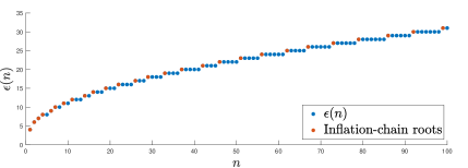
Figure 8: The function $\epsilon(n)$.

been $2+\sqrt{8n-4}$ (without rounding up), this would be obvious. But since $\epsilon(n)=\left\lceil 2+\sqrt{8n-4}\,\right\rceil$, it is a step function (with an infinite number of intervals), where the gap between all successive steps is exactly 1, except the gap between the two leftmost steps which is 2. This guarantees that despite the rounding, the minimum of $\epsilon(\left|Q_{1}\right|)+\epsilon(\left|Q_{2}\right|)$ occurs as claimed. Substituting this into Equation (2), and using the fact that $\epsilon(1)=4$, we see that $\epsilon(n-1)+2\leq\epsilon(n)$. However, we know [15] that $\epsilon(n)-\epsilon(n-1)\leq 1$ for $n\geq 3$, which is a contradiction. Thus, the deflated version of $Q$ cannot split into two parts unless it splits into two singleton cells, which is indeed the case for a minimal-perimeter polyomino of size 8, specifically, $D(\!\!\raisebox{-6.40186pt}{ \leavevmode\hbox to0pt{\vbox to0pt{\text{[drawing]}}} }\!\!)=\!\!\raisebox{-4.2679pt}{ \leavevmode\hbox to0pt{\vbox to0pt{\text{[drawing]}}} }$.

The same method can be used for showing that $D(Q)$ cannot be composed of more then two parts. Note that this proof does not hold for polyominoes of area which is not of the form $n+\epsilon(n)$, but it suffices for the use in Theorem 1. $\Box$

As mentioned earlier, it was already proven elsewhere [1, 15] that Premise 4 (roots of inflation chains) is fulfilled for the square lattice. Therefore, we proceed to showing that Premise 5 holds.

3.4 Premise 5: Convergence to a Minimum-Perimeter Polyomino

In this section, we show that starting from any polyomino $P$, and applying repeatedly some finite number of inflation steps, we obtain a polyomino $Q=Q(P)$, for which $\mathcal{P}(I(Q))=\mathcal{P}(Q)+4$. Let $R(Q)$ denote the diameter of $Q$, i.e., the maximal horizontal or vertical distance ($L^{\infty}$) between two cells of $Q$. The following lemma shows that some geometric features of a polyomino disappear after inflating it enough times.

Lemma 18

For any $k>R(Q)$, the polyomino $Q^{k}$ does not contain any (i) holes; (ii) cells of Type (d); or (iii) patterns of Type (z).

Proof: 

• Let $Q$ be a polyomino, and assume that $Q^{k}$ contains a hole. Consider a cell $c$ inside the hole, and let $c_{u}$ be the cell of $Q^{k}$ that lies immediately above it. (Note that since $c_{u}$ belongs to the border of $Q^{k}$, it is not a cell of $Q$.) Any cell that resides (not necessarily directly) below $c$ is closer to $c$ than to $c_{u}$. Since $c_{u}\in Q^{k}$, it ($c_{u}$) is closer than $c$ to $Q$, thus, there must be a cell of $Q$ (not necessarily directly) above $c$, otherwise $c_{u}$ would not belong to $Q^{k}$. The same holds for cells below, to the right, and to the left of $c$, thus, $c$ resides within the axis-aligned bounding box of the extreme cells of $Q$, and after $R(Q)$ steps, $c$ will be occupied, and any hole will be eliminated.

• Assume that there exists a polyomino $Q$, for which the polyomino $Q^{k}$ contains a cell of Type (d). Without loss of generality, assume that the neighbors of $c$ reside to its left and to its right, and denote them by $c_{\ell},c_{r}$, respectively. Denote by $c_{o}$ one of the cells whose inflation created $c_{\ell}$, i.e., a cell which belongs to $Q$ and is in distance of at most $k$ from $c_{\ell}$. In addition, denote by $c_{u},c_{d}$ the adjacent perimeter cells which lie immediately above and below $c$, respectively. The cell $c_{d}$ is not occupied, thus, its distance from $c_{o}$ is $k+1$, which means that $c_{o}$ lies in the same row as $c_{\ell}$. Assume for contradiction that $c_{o}$ lies in a row below $c_{\ell}$. Then, the distance between $c_{o}$ and $c_{d}$ is at most $k$, hence $c_{d}$ belongs to $Q^{k}$. The same holds for $c_{u}$; thus, cell $c_{o}$ must lie in the same row as $c_{\ell}$. Similar considerations show that $c_{o}$ must lie to the left of $c_{\ell}$, otherwise $c_{d}$ and $c_{u}$ would be occupied. In the same manner, one of the cells that originated $c_{r}$ must lie in the same row as $c_{r}$ on its right. Hence, any cell of Type (d) have cells of $Q$ to its right and to its left, and thus, it is found inside the bounding axis-aligned bounding box of $Q$, which will necessarily be filled with polyomino cells after $R(Q)$ inflation steps.

• Let $c$ be a Type-(z) perimeter cell of $Q^{k}$. Assume, without loss of generality, that the polyomino cells adjacent to it are to its left and to its right, and denote them by $c_{\ell}$ and $c_{r}$, respectively. Let $c_{o}$ denoted a cell whose repeated inflation has added $c_{\ell}$ to $Q^{k}$. (Note that $c_{o}$ might not be unique.) This cell must lie to the left of $c$, otherwise, it will be closer to $c$ than to $c_{\ell}$, and $c$ would not be a perimeter cell. In addition, $c_{o}$ must lie in the same row as $c_{\ell}$, for otherwise, by the same considerations as above, one of the cells above or below $c$ will be occupied. The same holds for $c_{r}$ (but to its right), thus, cells of Type (z) must reside between two original cells of $Q$, i.e., inside the bounding box of $Q$, and after $R(Q)$ inflation steps, all cells inside this box will become polyomino cells.

$\Box$

We can now conclude that inflating a polyomino $Q$ for $R(Q)$ times eliminates all holes and bridges, and, thus, the polyomino $Q^{k}$ will obey the equation $\left|\mathcal{P}(Q^{k})\right|=\left|\mathcal{B}(Q^{k})\right|+4$.

Lemma 19

Let $Q$ be a polyomino, and let $k=R(Q)$. We have that $\left|\mathcal{P}(Q^{k})\right|=\left|\mathcal{B}(Q^{k})\right|+4$.

Proof:  This follows at once from Lemma 18 and Theorem 16. $\Box$

4 Polyhexes

In this section, we show that the premises of Theorem 1 hold for the two-dimensional hexagonal lattice $\mathcal{H}$. The roadmap followed in this section is similar to the one used in Section 3. In this section, all the lattice-specific notations refer to $\mathcal{H}$.

4.1 Premise 1: Monotonicity

The first premise has been proven for $\mathcal{H}$ independently by Vainsencher and Bruckstien [17] and by Fülep and Sieben [10]. We will use the latter, stronger version which also includes a formula for $\epsilon(n)$.

Theorem 20

[10, Thm. $5.12$] $\epsilon(n)=\left\lceil\sqrt{12n-3}\,\right\rceil+3$.

Clearly, the function $\epsilon(n)$ is weakly-monotone increasing.

4.2 Premise 2: Constant Inflation

To show that the second premise holds, we analyze the different patterns that may appear in the border and perimeter of minimal-perimeter polyhexes. We can classify every border or perimeter cell by one of exactly 24 patterns, distinguished by the number and positions of their adjacent occupied cells. The 24 possible patterns are shown in Figure 9.

(a)

(b)

(c)

(d)

(e)

(f)

(g)

(h)

(i)

(j)

(k)

(l)

(o)

(p)

(q)

(r)

(s)

(t)

(u)

(v)

(w)

(x)

(y)

(z)

Figure 9: All possible patterns (up to symmetries) of border (first row) and perimeter (second row) cells. The gray cells are polyhex cells, while the white cells are perimeter cells. Each subfigure shows a cell in the middle, and the possible pattern of cells surrounding it.

Let us recall the equation subject of Lemma 12.

$$\left|\mathcal{P}(Q)\right|+e_{P}(Q)=\left|\mathcal{B}(Q)\right|+e_{B}(Q).$$

Our first goal is to express the excess of a polyhex $Q$ as a function of the numbers of cells of $Q$ of each pattern. We denote the number of cells of a specific pattern in $Q$ by $\#\leavevmode\hbox to0pt{\vbox to0pt{\text{[drawing]}}}$, where ‘’ is one of the 22 patterns listed in Figure 9. The excess (either border or perimeter excess) of Pattern  is denoted by $e(\leavevmode\hbox to0pt{\vbox to0pt{\text{[drawing]}}})$. (For simplicity, we omit the dependency on $Q$ in the notations of $\#\leavevmode\hbox to0pt{\vbox to0pt{\text{[drawing]}}}$ and $e(\leavevmode\hbox to0pt{\vbox to0pt{\text{[drawing]}}})$. This should be understood from the context.) The border excess can be expressed as $e_{B}(Q)=\sum_{\leavevmode\hbox to0pt{\vbox to0pt{\text{[drawing]}}}\in\{a,\dots,l\}}e(\leavevmode\hbox to0pt{\vbox to0pt{\text{[drawing]}}})\#\leavevmode\hbox to0pt{\vbox to0pt{\text{[drawing]}}}$, and, similarly, the perimeter excess can be expressed as $e_{P}(Q)=\sum_{\leavevmode\hbox to0pt{\vbox to0pt{\text{[drawing]}}}\in\{o,\dots,z\}}e(\leavevmode\hbox to0pt{\vbox to0pt{\text{[drawing]}}})\#\leavevmode\hbox to0pt{\vbox to0pt{\text{[drawing]}}}$. By plugging these equations into Equation (1), we obtain that

$$\left|\mathcal{P}(Q)\right|+\sum_{\leavevmode\hbox to0pt{\vbox to0pt{\text{[drawing]}}}\in\{o,\dots,z\}}e(\leavevmode\hbox to0pt{\vbox to0pt{\text{[drawing]}}})\#\leavevmode\hbox to0pt{\vbox to0pt{\text{[drawing]}}}=\left|\mathcal{B}(Q)\right|+\sum_{\leavevmode\hbox to0pt{\vbox to0pt{\text{[drawing]}}}\in\{a,\dots,l\}}e(\leavevmode\hbox to0pt{\vbox to0pt{\text{[drawing]}}})\#\leavevmode\hbox to0pt{\vbox to0pt{\text{[drawing]}}}~{}.$$ (3)

The next step of proving the second premise is showing that minimal-perimeter polyhexes cannot contain some of the 22 patterns. This will simplify Equation (3).

Lemma 21

(Analogous to Lemma 13.) A minimal-perimeter polyhex does not contains holes.

Proof:  Assume to the contrary that there exists a minimal-perimeter polyhex $Q$ that contains one or more holes, and let $Q^{\prime}$ be the polyhex obtained by filling one of the holes in $Q$. Clearly, $|Q^{\prime}|>|Q|$, and by filling the hole we eliminated some perimeter cells and did not create new perimeter cells. Hence, $\left|\mathcal{P}(Q^{\prime})\right|<\left|\mathcal{P}(Q)\right|$. This contradicts the fact that $\epsilon(n)$ is monotone increasing, as implied by Theorem 20. $\Box$

Another important observation is that minimal-perimeter polyhexes tend to be “compact.” We formalize this observation in the following lemma.

Recall the definition of a bridge from Section 3: A bridge is a cell whose removal unites two holes or renders the polyhex disconnected (specifically, Patterns (b), (d), (e), (g), (h), (j), and (k)). Similarly, a perimeter bridge is an empty cell whose addition to the polyhex creates a hole in it (specifically, Patterns (p), (r), (s), (u), (v), (x), and (y)).

Lemma 22

(Analogous to Lemma 15.) Minimal-perimeter polyhexes contain neither bridges nor perimeter bridges.

Proof:  Let $Q$ be a minimal-perimeter polyhex, and assume first that it contains a bridge cell $f$. By Lemma 21, since $Q$ does not contain holes, the removal of $f$ from $Q$ will break it into two or three disconnected polyhexes. We can connect these parts by translating one of them towards the other(s) by one cell. (In case of Pattern (h), the polyhex is broken into three parts, but then translating any of them towards the removed cell would make the polyhex connected again.) Locally, this will eliminate at least two perimeter cells created by the bridge. (This can be verified by exhaustively checking all the relevant patterns.) The size of the new polyhex, $Q^{\prime}$, is one less than that of $Q$, while the perimeter of $Q^{\prime}$ is smaller by at least two than that of $Q$. However, Theorem 20 implies that $\epsilon(n)-\epsilon(n-1)\leq 1$ for all $n\geq 3$, which is a contradiction to $Q$ being a minimal-perimeter polyhex.

Assume now that $Q$ contains a perimeter bridge. Filling the bridge will not increase the perimeter. (It might create one additional perimeter cell, which will be canceled out with the eliminated (perimeter) bridge cell.) In addition, it will create a hole in the polyomino. Then, filling the hole will create a polyhex with a larger size and a smaller perimeter, which is a contradiction to $\epsilon(n)$ being monotone increasing. $\Box$

As a consequence of Lemma 21, Pattern (o) cannot appear in any minimal-perimeter polyhex. In addition, Lemma 22 tells us that the Border Patterns (b), (d), (e), (g), (h), (j), and (k), as well as the Perimeter Patterns (p), (r), (s), (u), (v), (x), and (y) cannot appear in any minimal-perimeter polyhex. (Note that patterns (b) and (p) are not bridges by themselves, but the adjacent cell is a bridge, that is, the cell above the central cells in  and  are bridges.) Finally, Pattern (a) appears only in the singleton cell (the unique polyhex of size 1), which can be disregarded. Ignoring all these patterns, we obtain that

$$\left|\mathcal{P}(Q)\right|+3\#q+2\#t+\#w=\left|\mathcal{B}(Q)\right|+3\#c+2\#f+\#i.$$ (4)

Note that Patterns (l) and (z) have excess 0, and, hence, although they may appear in minimal-perimeter polyhexes, they do not contribute to the equation.

Consider a polyhex which contains only the six feasible patterns that contribute to the excess (those that appear in Equation (4)). Let $\xi$ denote the single polygon bounding the polyhex. We now count the number of vertices and the sum of internal angles of $\xi$ as functions of the numbers of appearances of the different patterns. In order to calculate the number of vertices of $\xi$, we first determine the number of vertices contributed by each pattern. In order to avoid multiple counting of a vertex, we associate each vertex to a single pattern. Note that each vertex of $\xi$ is surrounded by three (either occupied or empty) cells, out of which one is empty and two are occupied, or vise versa. We call the cell, whose type (empty or occupied) appears once (among the surrounding three cells), the “representative” cell, and count only these representatives. Thus, each vertex is counted exactly once.

For example, out of the six vertices surrounding Pattern (c), five vertices belong to the bounding polygon, but the representative cell of only three of them is the cell at the center of this pattern, thus, by our scheme, Pattern (c) contributes three vertices, each having a $2\pi/3$ angle. Similarly, only two of the four vertices in the configuration of Pattern (t), are represented by the cell at the center of this pattern. In this case, each vertex is the head of a $4\pi/3$ angle. To conclude, the total number of vertices of $\xi$ is

$$3\#c+2\#f+\#i+3\#q+2\#t+\#w,$$

and the sum of internal angles is

$$(3\#c+2\#f+\#i)2\pi/3+(3\#q+2\#t+\#w)4\pi/3.$$ (5)

On the other hand, it is known that the sum of internal angles is equal to

$$(3\#c+2\#f+\#i+3\#q+2\#t+\#w-2)\pi.$$ (6)

Equating the terms in Formulae (5) and (6), we obtain that

$$3\#c+2\#f+\#i=3\#q+2\#t+\#w+6.$$ (7)

Plugging this into Equation (4), we conclude that $\left|\mathcal{P}(Q)\right|=\left|\mathcal{B}(Q)\right|+6$, as required.

We also need to show that the second part of the second premise holds, that is, that if $Q$ is a minimal-perimeter polyhex, then $\left|\mathcal{P}(I(Q))\right|\leq\left|\mathcal{P}(Q)\right|+6$. To this aim, note that $\mathcal{B}(I(Q))\subset\mathcal{P}(Q)$, thus, it is sufficient to show that $\left|\mathcal{P}(I(Q))\right|\leq\left|\mathcal{B}(I(Q))\right|+6$. Obviously, Equation (3) holds for the polyhex $I(Q)$, hence, in order to prove the relation, we only need to prove the following lemma.

Lemma 23

If $Q$ is a minimal-perimeter polyhex, then $I(Q)$ does not contain any bridge.

Proof:  Assume to the contrary that $I(Q)$ contains a bridge. Then, the cell that makes the bridge must have been created in the inflation process. However, any cell $c\in I(Q)\backslash Q$ must have a neighboring cell $c^{\prime}\in Q$. All the cells adjacent to $c^{\prime}$ must also be part of $I(Q)$, thus, cell $c$ must have three consecutive neighbors around it, namely, $c^{\prime}$ and the two cells neighboring both $c$ and $c^{\prime}$. The only bridge pattern that fits this requirement is Pattern (j). However, this means that there must have been a gap of two cells in $Q$ that caused the creation of $c$ during the inflation of $Q$. Consequently, by filling the gap and the hole it created, we will obtain (see Figure 10) a larger polyhex with a smaller perimeter, which contradicts the fact that $Q$ is a minimal-perimeter polyhex. $\Box$

(a) $Q$

(b) $I(Q)$

(c) $Q^{\prime}$

Figure 10: The construction in Lemma 23 which shows that $I(Q)$ cannot contain a cell of Pattern $(j)$. Assuming that it does, by filling the hole in it, we obtain $Q^{\prime}$ which contradicts the perimeter-minimality of $Q$. (The marked cells in $Q^{\prime}$ are those added to $Q$.)

4.3 Premise 3: Deflation Resistance

We now show that deflating a minimal-perimeter polyhex results in another (smaller) valid polyhex. The intuition behind this condition is that a minimal-perimeter polyhex is “compact,” having a shape which does not become disconnected by deflation.

Lemma 24

For any minimal-perimeter polyhex $Q$, the shape $D(Q)$ is also a valid (connected) polyhex.

Proof:  The proof of this lemma is very similar to the first part of the proof of Lemma 22. Consider a minimal-perimeter polyhex $Q$. In order for $D(Q)$ to be disconnected, $Q$ must contain a bridge of either a single cell or two adjacent cells. A 1-cell bridge cannot be part of $Q$ by Lemma 22. The polyhex $Q$ can neither contain a 2-cell bridge.

(a)

(b)

(c)

Figure 11: An example for the construction in the proof of Lemma 22. The two-cell bridge is colored in red in (a). Then, in (b), the bridge is removed, and, in (c), the two parts are “glued” together.

Assume to the contrary that it does, as is shown in Figure 11(a). Then, removing the bridge (see Figure 11(b)), and then connecting the two pieces (by translating one of them towards the other by one cell along a direction which makes a $60^{\circ}$ angle with the bridge), creates (Figure 11(c)) a polyhex whose size is smaller by two than that of the original polyhex, and whose perimeter is smaller by at least two (since the perimeter cells adjacent to the bridge disappear). The new polyhex is valid, that is, the translation by one cell of one part towards the other does not make any cells overlap, otherwise there is a hole in the original polyhex, which is impossible for a minimal-perimeter polyhex by Lemma 21. However, we reached a contradiction since for a minimal-perimeter polyhex of size $n\geq 7$, we have that $\epsilon(n)-\epsilon(n-2)\leq 1$. Finally, it is easy to observe by a tedious inspection that the deflation of any polyhex of size less than 7 results in the empty polyhex. $\Box$

In conclusion, we have shown that all the premises of Theorem 1 are satisfied for the hexagonal lattice, and, therefore, inflating a set of all the minimal-perimeter polyhexes of a certain size yields another set of minimal-perimeter polyhexes of another, larger, size. This result is demonstrated in Figure 12.

Figure 12: A demonstration of Theorem 1 for polyhexes. The top row contains all polyhexes in $M_{9}$ (minimal-perimeter polyhexes of size 9), while the bottom row contains their inflated versions, all the members of $M_{23}$.

We also characterized inflation-chain roots of polyhexes. As is mentioned above, the premises of Theorems 1 and 7 are satisfied for polyhexes [17, 15], and, thus, the inflation-chain roots are those who have the minimum size for a given minimal-perimeter size. An easy consequence of Theorem 20 is that the formula $\left\lfloor\frac{(p-4)^{2}}{12}+\frac{5}{4}\right\rfloor$ generates all these inflation-chain roots. This result is demonstrated in Figure 13.

[scale=0.40]minpH_roots

Figure 13: The relation between the minimum perimeter of polyhexes, $\epsilon(n)$, and the inflation-chain roots. The points represent the minimum perimeter of a polyhex of size $n$, and sizes which are inflation-chain roots are colored in red. The arrows show the mapping between sizes of minimal-perimeter polyhexes (induced by the inflation operation) and demonstrate the proof of Theorem 6.

As in the case of polyominoes, and as was mentioned earlier, it was already proven elsewhere [17, 10] that Premise 4 (roots of inflation chains) is fulfilled for the hexagonal lattice. Therefore, we proceed to showing that Premise 5 holds.

4.4 Premise 5: Convergence to a Minimum-Perimeter Polyomino

Similarly to polyominoes, we now show that starting from a polyhex $Q$ and applying repeatedly a finite number, $k$, of inflation steps, we obtain a polyhex $Q^{k}=I^{k}(Q)$, for which $\mathcal{P}(I(Q^{k}))=\mathcal{P}(Q^{k})+6$. Let $R(Q)$ denote the diameter of $Q$, i.e., the maximal distance between two cells of $Q$ when projected onto one of the three main axes. As in the case of polyominoes, some geometric features of $Q$ will disappear after $R(Q)$ inflation steps.

Lemma 25

(Analogous to Lemma 18.) For any $k>R(Q)$, the polyhex $Q^{k}$ does not contain any (i) holes; (ii) polyhex bridge cells; or (iii) perimeter bridge cells.

Proof: 

• The proof is identical to the proof for polyominoes.

• After $R(Q)$ inflation steps, the obtained polyhex is clearly connected. If at this point there exists a bridge cell, then it must have been created in the last inflation step since after further steps, this cell would cease being a bridge cell. If during this inflation step, that eliminates the mentioned bridge, another bridge is created then its removal will not render the polyomino disconnected (since it was already connected before applying the inflation step), thus, it must have created a hole in the polyhex, in contradiction to the previous clause.

• We will present here a version of the analogue proof for polyominoes, adapted for polyhexes. Let $c$ be a perimeter bridge cell of $Q^{k}$. Assume, without loss of generality, that two of the polyhex cells adjacent to it are above and below it, and denote them by $c_{1}$ and $c_{2}$, respectively. The cell whose inflation resulted in adding $c_{1}$ to the polyhex $c_{1}$, denoted by $c_{o}$, must reside above $c$, otherwise, it would be closer to $c$ than to $c_{1}$, and $c$ would not be a perimeter cell. The same holds for $c_{2}$ (below $c$), thus, any perimeter bridge cell must reside between two original cells of $Q$. Hence, after $R(Q)$ inflation steps, all such cells will become a polyhex cells.

$\Box$

Lemma 26

(Analogous to Lemma 19.) After $k=R(Q)$ inflation steps, the polyhex $Q^{k}$ will obey $\left|\mathcal{P}(Q^{k})\right|=\left|\mathcal{B}(Q^{k})\right|+6$.

Proof:  This follows at once from Lemma 25 and Equation 7. $\Box$

5 Polyiamonds

Polyiamonds are sets of edge-connected triangles on the regular triangular lattice. Unlike the square and the hexagonal lattice, in which all cells are identical in shape and in their role, the triangular lattice has two types of cells, which are seen as a left and a right pointing arrows ( , ). Due to this complication, inflating a minimal-perimeter polyiamond does not necessarily result in a minimal-perimeter polyiamond. Indeed, the second premise of Theorem 1 does not hold for polyiamonds. This fact is not surprising, since inflating minimal-perimeter polyiamonds creates “jaggy” polyiamonds whose perimeter is not minimal. Figures 14(a,b) illustrate this phenomenon.

(a) $Q$

(b) $I(Q)$

(c) $Q^{\prime}$

Figure 14: An example of inflating polyiamonds. The polyiamond $Q$ is of a minimum perimeter, however, its inflated version, $I(Q)$ is not of a minimum perimeter. The polyiamond $Q^{\prime}$, obtained by adding to $Q$ all the cells sharing a vertex with $Q$, is a minimal-perimeter polyiamond.

However, we can fix this situation in the triangular lattice by modifying the definition of the perimeter of a polyiamond so that it it would include all cells that share a vertex (instead of an edge) of the boundary of the polyiamond. Under the new definition, Theorem 1 holds. The reason for this is surprisingly simple: The modified definition merely mimics the inflation of animals on the graph dual to that of the triangular lattice. (Recall that graph duality maps vertices to faces (cells), and vice versa, and edges to edges.) However, the dual of the triangular lattice is the hexagonal lattice, for which we have already shown in Section 4 that all the premises of Theorem 1 hold. Thus, applying the modified inflation operator in the triangular lattice induces a bijection between sets of minimal-perimeter polyiamonds. This relation is demonstrated in Figure 14.

6 Conclusion

In this paper, we show that the inflation operation induces a bijection between sets of minimal-perimeter animals on any lattice which satisfies three conditions. We demonstrate this result on three planar lattices: the square, hexagonal, and also the triangular (with a modified definition of the perimeter). The most important contribution of this paper is the application of our result to polyhexes. Specifically, the phenomenon of the number of isomers of a benzenoid hydrocarbons remaining unchanged under circumscribing, which was observed in the literature of chemistry more than 30 years ago but has never been proven till now.

However, we do not believe that this set of conditions is necessary. Empirically, it seems that by inflating all the minimal-perimeter polycubes (animals on the 3-dimensional cubical lattice) of a given size, we obtain all the minimal-perimeter polycubes of some larger size. However, the second premise of Theorem 1 does not hold for this lattice. Moreover, we believe that as stated, Theorem 1 applies only to 2-dimensional lattices! A simple conclusion from Lemma 3 is that if the premises of Theorem 1 hold for animals on a lattice $\mathcal{L}$, then $\epsilon_{\mathcal{L}}(n)=\Theta(\sqrt{n})$. We find it is reasonable to assume that for a $d$-dimensional lattice $\mathcal{L}_{d}$, the relation between the size of a minimal-perimeter animal and its perimeter is roughly equal to the relation between a $d$-dimensional sphere and its surface area. Hence, we conjecture that $\epsilon^{\mathcal{L}_{d}}(n)=\Theta(n^{1-1/d})$, and, thus, Theorem 1 is not suitable for higher dimensions.

References

- [1] Y. Altshuler, V. Yanovsky, D. Vainsencher, I. Wagner, and A. Bruckstein. On minimal perimeter polyminoes. In Discrete Geometry for Computer Imagery, 13th International Conference, Szeged, Hungary, pages 17–28. Springer, October 2006.
- [2] A. Asinowski, G. Barequet, and Y. Zheng. Enumerating polyominoes with fixed perimeter defect. In Proc. 9th European Conf. on Combinatorics, Graph Theory, and Applications, volume 61, pages 61–67, Vienna, Austria, August 2017. Elsevier.
- [3] A. Asinowski, G. Barequet, and Y. Zheng. Polycubes with small perimeter defect. In Proc. 29th Ann. ACM-SIAM Symp. on Discrete Algorithms, pages 93–100, New Orleans, LA, January 2018.
- [4] G. Barequet and G. Ben-Shachar. Algorithms for counting minimal-perimeter lattice animals. Under submission., 2020.
- [5] J. Brunvoll and S. Cyvin. What do we know about the numbers of benzenoid isomers? Zeitschrift für Naturforschung A, 45(1):69–80, 1990.
- [6] S. J. Cyvin and J. Brunvoll. Series of benzenoid hydrocarbons with a constant number of isomers. Chemical Physics Letters, 176(5):413–416, 1991.
- [7] J. Dias. Handbook of polycyclic dydrocarbons. Part A: Benzenoid hydrocarbons. Elsevier Science Pub. Co. Inc., New York, NY, 1987.
- [8] J. Dias. New general formulations for constant-isomer series of polycyclic benzenoids. Polycyclic Aromatic Compounds, 30:1–8, February 2010.
- [9] M. Eden. A two-dimensional growth process. Dynamics of Fractal Surfaces, 4:223–239, 1961.
- [10] G. Fülep and N. Sieben. Polyiamonds and polyhexes with minimum site-perimeter and achievement games. The Electronic Journal of Combinatorics, 17(1):65, 2010.
- [11] F. Harary and H. Harborth. Extremal animals. J. of Combinatorics, Information, and System Sciences, 1(1):1–8, 1976.
- [12] I. Jensen and A. Guttmann. Statistics of lattice animals (polyominoes) and polygons. J. of Physics A: Mathematical and General, 33(29):L257, 2000.
- [13] S. Mertens. Lattice animals: A fast enumeration algorithm and new perimeter polynomials. Journal of Statistical Physics, 58(5):1095–1108, March 1990.
- [14] D. H. Redelmeier. Counting polyominoes: yet another attack. Discrete Mathematics, 36(2):191–203, 1981.
- [15] N. Sieben. Polyominoes with minimum site-perimeter and full set achievement games. European J. of Combinatorics, 29(1):108–117, 2008.
- [16] H. Temperley. Combinatorial problems suggested by the statistical mechanics of domains and of rubber-like molecules. Physical Review, 103(1):1, 1956.
- [17] D. Vainsencher and A. M. Bruckstein. On isoperimetrically optimal polyforms. Theor. Comput. Sci., 406(1-2):146–159, 2008.
- [18] D.-L. Wang and P. Wang. Discrete isoperimetric problems. SIAM Journal on Applied Mathematics, 32(4):860–870, 1977.