Prospects of cooling a mechanical resonator with a transmon qubit in c-QED setup

Abstract

Hybrid devices based on the superconducting qubits have emerged as a promising platform for controlling the quantum states of macroscopic resonators. The nonlinearity added by a qubit can be a valuable resource for such control. Here we study a hybrid system consisting of a mechanical resonator longitudinally coupled to a transmon qubit. The qubit readout can be done by coupling to a readout mode like in c-QED setup. The coupling between the mechanical resonator and transmon qubit can be implemented by modulation of the SQUID inductance. In such a tri-partite system, we analyze the steady-state occupation of the mechanical mode when all three modes are dispersively coupled. We use the quantum-noise and the Lindblad formalism to show that the sideband cooling of the mechanical mode to its ground state is achievable. We further experimentally demonstrate that measurements of the thermomechanical motion is possible in the dispersive limit, while maintaining a large coupling between qubit and mechanical mode. Our theoretical calculations suggest that single-photon strong coupling is within the experimental reach in such hybrid devices.

I Introduction:

Control over the quantum states of a mechanical resonator by coupling them to optical modes can have several potential applications in the field of quantum technologies [1]. The traditional cavity-optomechanics based approach of coupling a mechanical resonator to an optical mode via the radiation-pressure interaction has been quite successful [2, 3, 4, 5, 6, 7, 8, 9]. While the radiation-pressure mediated coupling in such devices is nonlinear, its magnitude is usually small in most applications. Further, due to the dispersive interaction, the effects originating from the Kerr-term are strongly suppressed [10, 11].

To mitigate the limitations of linear cavity optomechanics, hybrid devices based on the strong nonlinearity of qubits have been proposed and developed [12, 13, 14]. These proposals explore their performance from the sideband cooling of the mechanical resonator [15] to the matter-interferometry [16], while considering a wide range of two-level systems such as superconducting qubits [15, 17, 18, 19, 20, 21, 22], quantum-dots [23], and nitrogen vacancy defects in diamond [24]. Particularly, in the microwave domain, experimental realization of several hybrid devices have been shown using the nonlinearity of a superconducting qubit [25], Josephson capacitance [26, 27], Josephson inductance [28, 29, 30, 31], and piezo-electricity [32, 33].

Among these different schemes, the electromechanical coupling stems from charge or flux modulation, and its tunability is controlled by the external applied magnetic field. Recently, the magnetic flux-mediated coupling approach have shown promising experimental results [28]. These systems have demonstrated large electromechanical coupling [29, 30, 31], four-wave-cooling of the mechanical resonator to near the quantum ground state [34], and Lorentz-force induced backaction on the mechanical resonator [35].

Motivated by the progress on flux-mediated approach, here we investigate a coupled three-mode system consisting of a mechanical mode, transmon qubit, and a readout cavity. From the practical point of view, the additional readout cavity is useful ingredient to consider as it allows the quantum non-demolishing (QND) measurement of qubit mode in circuit-QED setup [36, 37]. While a mechanical mode coupled to a two-level system has been studied extensively in the past [15, 38, 17, 12, 39], the focus of our investigation has been on treating the transmon qubit as a weakly anharmonic oscillator. In addition, we theoretically and experimentally address the readout of the mechanical mode when transmon is detuned far away from the readout cavity. This regime is particularly important as large electromechanical coupling with the qubit mode can be achieved. Using the quantum-Langevin equation of motion [40], and Lindblad formalism [41], we analyze the possibility of sideband cooling of the mechanical resonator. Experimentally, we use a two-tone method to measure the thermo-mechanical motion, and compare it with analytical results.

This paper is organised as follows: In part II, we discuss the theoretical model of the three coupled modes. We solve the system’s equations of motion in part III. The analytical solution of the system is analyzed in part IV, where we have shown the possibility of cooling the mechanical resonator. In the part V, we show experimental and analytical results discussing the detection of mechanical motion in the dispersive regime of the cavity and the qubit mode. We summarize and conclude our discussion in part VI.

II Theoretical model:

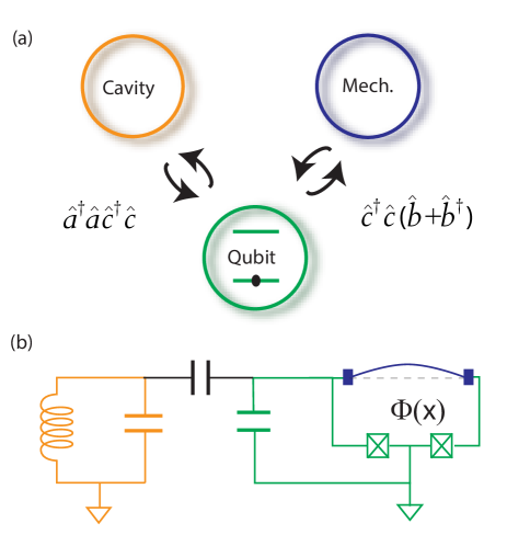
Figure 1: (a) A conceptual schematic of the three-mode hybrid device showing a linear cavity coupled to a qubit which in turn couples to a mechanical resonator. A direct coupling between the cavity and the mechanical mode is not considered. (b) A possible implementation using a frequency tunable transmon qubit, where coupling to mechanical mode is achieved by embedding it the SQUID loop and by applying a constant magnetic field. A magnetic field perpendicular to the SQUID loop couples the in-plane mechanical mode to the qubit, while parallel magnetic field couples the qubit to the out-of-plane mechanical mode.

We consider a coupled system where the mechanical mode modulates the transmon qubit frequency, therefore resulting in a longitudinal coupling. Such coupling between transmon qubit and the mechanical resonator can be implemented by embedding a mechanical resonator into the SQUID loop of the qubit. In addition, the qubit couples to a linear mode (the readout cavity) transversely as in the circuit-QED setup. A schematic diagram of the system and a possible implementation with the equivalent circuit diagram are shown in the Fig. 1 (a) and (b).

Using the dispersive approximation between the transmon and the readout cavity, we arrive at the following system Hamiltonian:

$$\hat{\mathcal{H}}_{0}=\omega_{c}\hat{a}^{\dagger}\hat{a}+\omega_{q}\hat{c}^{\dagger}\hat{c}-\frac{\alpha_{q}}{2}\hat{c}^{\dagger}\hat{c}^{\dagger}\hat{c}\hat{c}+\omega_{m}\hat{b}^{\dagger}\hat{b}\\ +\chi~{}\hat{a}^{\dagger}\hat{a}\hat{c}^{\dagger}\hat{c}+g_{0}~{}\hat{c}^{\dagger}\hat{c}(\hat{b}+\hat{b}^{\dagger}),$$ (1)

where $\hat{a}$($\hat{a}^{\dagger}$), $\hat{c}$($\hat{c}^{\dagger}$), $\hat{b}$($\hat{b}^{\dagger}$) are the annihilation(creation) operators for the cavity, qubit and the mechanical mode of frequency $\omega_{c}$, $\omega_{q}$, $\omega_{m}$, respectively. The Kerr-nonlinearity of the transmon is denoted as $\alpha_{q}$. The last two terms are the interaction terms between the modes, where the dispersive coupling between the qubit and the cavity is $\chi$. The radiation-pressure type coupling between the transmon and the mechanical mode is denoted by the single photon coupling rate $g_{0}$.

Two additional drive terms of amplitude $\delta$ and $\epsilon$ at frequency of $\omega_{L}$ (near $\omega_{c}$) and $\omega_{d}$ (near $\omega_{q}$) are added to the Hamiltonian. We can write the drive Hamiltonian as,

$$\hat{\mathcal{H}}_{d}=\delta~{}(\hat{a}~{}e^{+{i}\omega_{L}t}+\hat{a}^{\dagger}~{}e^{-{i}\omega_{L}t})+\epsilon~{}(\hat{c}~{}e^{+{i}\omega_{d}t}+\hat{c}^{\dagger}~{}e^{-{i}\omega_{d}t}).$$ (2)

By carrying out rotating frame transformations, given by the unitary operators $U^{a}=\exp{\left[{i}\omega_{L}\hat{a}^{\dagger}\hat{a}t\right]}$ and $U^{c}=\exp{\left[{i}\omega_{d}\hat{c}^{\dagger}\hat{c}t\right]}$, the transformed Hamiltonian can be written as,

$$\hat{\mathcal{H}}=-\Delta_{c}\hat{a}^{\dagger}\hat{a}-\Delta_{q}\hat{c}^{\dagger}\hat{c}-\frac{\alpha_{q}}{2}\hat{c}^{\dagger}\hat{c}^{\dagger}\hat{c}\hat{c}+\omega_{m}\hat{b}^{\dagger}\hat{b}+\chi~{}\hat{a}^{\dagger}\hat{a}\hat{c}^{\dagger}\hat{c}\\ +g_{0}~{}\hat{c}^{\dagger}\hat{c}(\hat{b}+\hat{b}^{\dagger})+\delta~{}(\hat{a}+\hat{a}^{\dagger})+\epsilon~{}(\hat{c}+\hat{c}^{\dagger}),$$ (3)

where $\Delta_{c}=\omega_{L}-\omega_{c}$ and $\Delta_{q}=\omega_{d}-\omega_{q}$. The transformed Hamiltonian is time-independent in this frame of rotation. For further analysis, we shift the frame to mean field using the following displacement transformation,

$$\mathcal{D}(\alpha,\mu,\beta)=\exp{\left[\alpha(\hat{a}-\hat{a}^{\dagger})+\mu(\hat{c}-\hat{c}^{\dagger})+\beta(\hat{b}-\hat{b}^{\dagger})\right]},$$ (4)

where $\alpha$, $\mu$, $\beta$ are real scalar quantities. For a particular choice of $\alpha=\bar{\alpha}$, $\mu=\bar{\mu}$ and $\beta=\bar{\beta}$, all the drive terms (terms proportional to $\hat{a}+\hat{a}^{\dagger}$, $\hat{b}+\hat{b}^{\dagger}$, and $\hat{c}+\hat{c}^{\dagger}$) get cancelled. After dropping the third and higher order terms, we arrive at the following effective Hamiltonian,

$$\hat{\mathcal{H}^{\prime}}\approx-\tilde{\Delta}_{c}\hat{a}^{\dagger}\hat{a}-\tilde{\Delta}_{q}\hat{c}^{\dagger}\hat{c}-\eta(\hat{c}^{2}+\hat{c}^{\dagger 2})+\omega_{m}\hat{b}^{\dagger}\hat{b}\\ +J(\hat{a}+\hat{a}^{\dagger})(\hat{c}+\hat{c}^{\dagger})+g(\hat{c}+\hat{c}^{\dagger})(\hat{b}+\hat{b}^{\dagger}),$$ (5)

where $\tilde{\Delta}_{c}=\Delta_{c}-\chi\bar{\mu}^{2}$, $\tilde{\Delta}_{q}=\Delta_{q}+2\alpha_{q}\bar{\mu}^{2}-\chi\bar{\alpha}^{2}-2g_{0}\bar{\beta}$, $\eta=\frac{\alpha_{q}\bar{\mu}^{2}}{2}$, $J=\chi\bar{\alpha}\bar{\mu}$ and $g=g_{0}\bar{\mu}$. It might be important to underline here that the coupling rates $g$ and $J$ as defined above are the scaled coupling rates. They show the scaling with drive tone amplitude similar to the case in linear optomechanical device.

III Equations of motion:

Dynamics of the system depends on various decay rates associated with different modes and drive amplitudes. We write the equations of motion for the field operators while incorporating all the noise operators and decay rates as,

$$\dot{\hat{a}} =-{i}\left[\hat{a},\hat{\mathcal{H}^{\prime}}\right]-\frac{\kappa}{2}\hat{a}+\sqrt{\kappa_{ex}}~{}\hat{a}_{in}+\sqrt{\kappa_{0}}~{}\hat{f}_{in},$$ (6a)

$$\dot{\hat{c}} =-{i}\left[\hat{c},\hat{\mathcal{H}^{\prime}}\right]-\frac{\Gamma}{2}\hat{c}+\sqrt{\Gamma_{ex}}~{}\hat{c}_{in}+\sqrt{\Gamma_{0}}~{}\hat{\xi}_{in},$$ (6b)

$$\dot{\hat{b}} =-{i}\left[\hat{b},\hat{\mathcal{H}^{\prime}}\right]-\frac{\gamma_{m}}{2}\hat{b}+\sqrt{\gamma_{m}}~{}\hat{b}_{in},$$ (6c)

where $\hat{a}_{in}$, $\hat{c}_{in}$, $\hat{b}_{in}$, $\hat{f}_{in}$, $\hat{\xi}_{in}$ are noise operators of cavity, qubit and mechanical mode, respectively. The mechanical energy dissipation rate is $\gamma_{m}$. The internal, external and total cavity (qubit) dissipation rates are $\kappa_{0}$ ($\Gamma_{0}$), $\kappa_{ex}$ ($\Gamma_{ex}$), and $\kappa$ ($\Gamma$), respectively.

This set of equations can be easily solved by performing a Fourier transformation, defined as $x[\omega]=\mathcal{F}\left[x(t)\right]=\int_{-\infty}^{+\infty}x(t)\mathrm{e}^{{i}\omega t}\mathrm{d}t$, of the equations. We now define a field vector $u[\omega]=\begin{bmatrix}\hat{a}[\omega]&(\hat{a}^{\dagger})[\omega]&\hat{c}[\omega]&(\hat{c}^{\dagger})[\omega]&\hat{b}[\omega]&(\hat{b}^{\dagger})[\omega]\end{bmatrix}^{T}$ and evaluate its governing equation of the form,

$$u[\omega]=(-{i}\omega\mathbb{1}-A)^{-1}~{}r[\omega]=\mathcal{B}~{}r[\omega],$$ (7)

where,

$$r[\omega]=\begin{bmatrix}\sqrt{\kappa_{ex}}~{}\hat{a}_{in}[\omega]+\sqrt{\kappa_{0}}~{}\hat{f}_{in}[\omega]\\ \sqrt{\kappa_{ex}}~{}(\hat{a}_{in}^{\dagger})[\omega]+\sqrt{\kappa_{0}}~{}(\hat{f}_{in}^{\dagger})[\omega]\\ \sqrt{\Gamma_{ex}}~{}\hat{c}_{in}[\omega]+\sqrt{\Gamma_{0}}~{}\hat{\xi}_{in}[\omega]\\ \sqrt{\Gamma_{ex}}~{}(\hat{c}_{in}^{\dagger})[\omega]+\sqrt{\Gamma_{0}}~{}(\hat{\xi}_{in}^{\dagger})[\omega]\\ \sqrt{\gamma_{m}}~{}\hat{b}_{in}[\omega]\\ \sqrt{\gamma_{m}}~{}(\hat{b}_{in}^{\dagger})[\omega]\end{bmatrix}$$ (8)

The matrix $\mathcal{B}$ can be calculated from Eq. (5) and Eq. (6), as

$$\mathcal{B}=\begin{bmatrix}1/\chi_{c}&0&{i}J&{i}J&0&0\\ 0&1/\tilde{\chi}_{c}&-{i}J&-{i}J&0&0\\ {i}J&{i}J&1/\chi_{q}&-2{i}\eta&{i}g&{i}g\\ -{i}J&-{i}J&2{i}\eta&1/\tilde{\chi}_{q}&-{i}g&-{i}g\\ 0&0&{i}g&{i}g&1/\chi_{m}&0\\ 0&0&-{i}g&-{i}g&0&1/\tilde{\chi}_{m}\end{bmatrix}^{\scalebox{1.0}{-1}}.$$ (9)

All $\chi$’s in the matrix represent the susceptibility of the modes, defined as,

$$\chi_{c}[\omega]=\frac{1}{-{i}\omega-{i}\tilde{\Delta}_{c}+\frac{\kappa}{2}};~{}\tilde{\chi}_{c}[\omega]=\frac{1}{-{i}\omega+{i}\tilde{\Delta}_{c}+\frac{\kappa}{2}}$$

$$\chi_{q}[\omega]=\frac{1}{-{i}\omega-{i}\tilde{\Delta}_{q}+\frac{\Gamma}{2}};~{}\tilde{\chi}_{q}[\omega]=\frac{1}{-{i}\omega+{i}\tilde{\Delta}_{q}+\frac{\Gamma}{2}}$$

$$\chi_{m}[\omega]=\frac{1}{-{i}\omega+{i}\omega_{m}+\frac{\gamma_{m}}{2}};~{}\tilde{\chi}_{m}[\omega]=\frac{1}{-{i}\omega-{i}\omega_{m}+\frac{\gamma_{m}}{2}}.$$

From Eq. 7, we can solve for the field operators. Further, we define the spectrum of any mode as,

$$S_{\mathcal{O}}(\omega)=\frac{1}{2\pi}\int_{-\infty}^{+\infty}\langle(\hat{\mathcal{O}}[\omega^{\prime}])^{\dagger}\hat{\mathcal{O}}[\omega]\rangle\mathrm{d}\omega^{\prime}.$$ (10)

Eq. 10 and the solution of field operators can be used to get the spectrum of the modes. The detailed calculations and the correlators of noise operators are given in Appendix A. The calculated spectrum as follows,

$$S_{\text{x}}(\omega)\Big{|}_{\text{x}\epsilon\{1,3,5\}}=n_{m}^{i}\gamma_{m}(|\mathcal{B}_{\text{x}5}[\omega]|^{2}+|\mathcal{B}_{\text{x}6}[\omega]|^{2})+\\ \kappa|\mathcal{B}_{\text{x}2}[\omega]|^{2}+\Gamma|\mathcal{B}_{\text{x}4}[\omega]|^{2}+\gamma_{m}|\mathcal{B}_{\text{x}6}[\omega]|^{2},$$ (11)

where $n_{m}^{i}$ is the initial phonon occupation in the mechanical mode. The indexing $\{S_{1},S_{3},S_{5}\}$ maps to the spectrum of cavity, qubit and mechanics as $\{S_{a},S_{c},S_{b}\}$, respectively.

IV Spectrum of the qubit and the mechanical mode

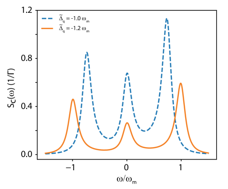
Figure 2: Plot of the qubit spectrum for two different values of drive detunings, $\tilde{\Delta}_{q}=-1.0~{}\omega_{m}$ and $\tilde{\Delta}_{q}=-1.2~{}\omega_{m}$. The parameters used for the plots: $\tilde{\Delta}_{c}=0$, $\omega_{m}=2\pi\times 6$ MHz, $J=2\pi\times 0.8$ MHz, $g=2\pi\times 2$ kHz, $\kappa=2\pi\times 4$ MHz, $\omega_{m}/\Gamma=5$, $\gamma=2\pi\times 6$ Hz, and $\eta=2\pi\times 2$ MHz.

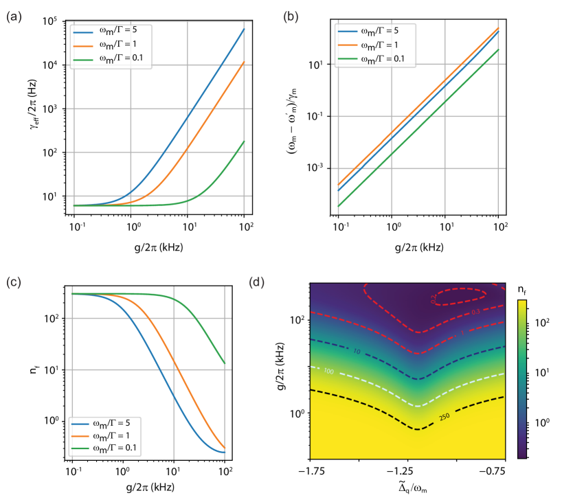
Figure 3: Cooling of the mechanical mode: The spectrum of the mechanical mode is analyzed to characterize the effect of back action arising from the drive tone near the qubit frequency $\omega_{q}$. The extracted parameters for effective mechanical linewidth and shift in the mechanical resonant frequency as the electromechanical coupling between the qubit and the mechanical mode is varied, are shown in (a) and (b). Panel (c) shows the final phonon occupancy of the mechanical mode. It is extracted by calculating the area under the Lorentzian in mechanical spectrum. For large qubit-mechanics coupling a final phonon occupation well-below 1 can be achieved for various sideband parameters. (d) Final phonon occupancy as a function of qubit-mechanics coupling and scaled detuning between the drive and the qubit frequency for $\omega_{m}/\Gamma=5$. The parameters used for the plots are: $\tilde{\Delta}_{c}=0$, $\omega_{m}=2\pi\times 6$ MHz, $J=2\pi\times 0.8$ MHz, $\eta=2\pi\times 2$ MHz, $\kappa=2\pi\times 4$ MHz, $\gamma=2\pi\times 6$ Hz, $n_{m}^{i}=300$. For the plot in panel (a), (b), and (c), we use $\tilde{\Delta}_{q}=-1.2~{}\omega_{m}$ as the detuning.

In this section, we discuss the best cooling scenario of the mechanical resonator by inspecting the qubit spectrum. Fig. 2 shows the spectrum of the transmon qubit for two different detuning of the drive tone,($\tilde{\Delta}_{q}=-1.0~{}\omega_{m}$ and $\tilde{\Delta}_{q}=-1.2~{}\omega_{m}$). In presence of a the nearly red detuned drive on qubit mode, its spectrum becomes asymmetric. The cooling rate is calculated from the asymmetry of the spectrum, which is large for a specific drive position. In the weak coupling regime ($g<<\Gamma$), the cooling rate for the mechanical resonator is given by $\Gamma_{c}=2[g^{2}(S_{c}(\omega_{m})-S_{c}(-\omega_{m}))+\gamma_{m}]$ [17, 12]. The optimum cooling rate, as seen from Fig. 2, is a function of the position of the drive [17]. Unlike a linear cavity as a bath for cooling, the cooling rate of a mechanical resonator for an anharmonic oscillator (the qubit) depends on the position of the cooling tone applied and the anharmonicity of the resonator mode. This is a direct consequence of the Kerr-term. In the steady state, the final phonon occupancy can be calculated from the cooling rate and the qubit spectrum as,

$$n_{f}=2\frac{n_{m}^{i}\gamma_{m}}{\Gamma_{c}}+2g^{2}\frac{S_{c}(-\omega_{m})}{\Gamma_{c}}.$$ (12)

To further understand the backaction on the mechanical resonator due to a drive on the qubit mode, we compute the mechanical spectrum $S_{b}(\omega)$. In the steady state, the mean phonon occupancy of the mechanical mode can be calculated as $n_{f}=\frac{1}{2\pi}\int S_{b}(\omega)d\omega$, which is the area under the Lorentzian in the mechanical mode spectrum. While it is possible to reduce the expression of the mechanical spectrum to a Lorentzian form, we find it more efficient to compute the spectrum and carry out a numerical fit to extract the effective linewidth and the effective resonant frequency. Fig. 3(a) and Fig. 3(b) show the linewidth broadening and resonant frequency shift of the mechanical mode, for a red detuned ($\tilde{\Delta}_{q}=-1.2~{}\omega_{m}$) qubit drive. The back-action on the mechanical resonator from the drive on qubit is reflected in the change of mechanical frequency and an increase in the effective linewidth. The final phonon occupation is plotted in Fig. 3(c) for different value of sideband parameter $\omega_{m}/\Gamma$. It is evident from the figure that in the steady driving of the qubit, the final phonon occupancy strongly depends on sideband parameter $\omega_{m}/\Gamma$. A larger value of sideband parameter offers better cooling of the mechanical mode. It is important to underline here that the cooling to the quantum ground state of the mechanical resonator is possible well before entering the strong coupling regime, $g~{}\gtrsim\text{max}~{}(\Gamma,\kappa)$.

To gain insight into the spectrum calculation, we consider a simpler case when qubit anharmonicity is set to zero $\eta=0$, and it is being driven at the lower mechanical sideband $\tilde{\Delta}_{q}=-\omega_{m}$. With these parameters and Eq. 10, the mechanical spectrum can be approximately written as,

$$S_{b}(\omega)=\frac{n_{m}^{i}\gamma_{m}\Gamma^{2}/(\Gamma^{2}-8g^{2})}{(\omega-\omega_{m})^{2}+\frac{(4g^{2}+\gamma_{m}\Gamma)^{2}}{4(\Gamma^{2}-8g^{2})}}.$$ (13)

From this simplified expression of the mechanical spectrum, we can write the effective line-width of the mechanical resonator as, $\gamma_{eff}=\frac{4g^{2}+\gamma_{m}\Gamma}{\sqrt{\Gamma^{2}-8g^{2}}}\simeq\gamma_{m}(C+1)$, where $C=\frac{4g^{2}}{\gamma_{m}\Gamma}$ is defined as the cooperativity. Similarly, the final mean phonon occupation can be written as, $n_{f}=\frac{n_{m}^{i}\gamma_{m}\Gamma^{2}}{4g^{2}+\gamma_{m}\Gamma}\frac{1}{\sqrt{\Gamma^{2}-8g^{2}}}\simeq\frac{n_{m}^{i}}{1+C}$ for $\Gamma\gg g$. We note that in the limit of zero anharmonicity and weak coupling, the results are consistent with that obtain from linear cavity optomechanics [2].

For the model Hamiltonian given by Eq. 5, the mean phonon-occupation can also be obtained by solving Lindblad master equation. Here, we obtain the equations of motion for the expectation values of mode operators and solve for the steady-state solutions. From this formalism, we calculate the steady-state occupancy in the mechanical mode for the various drive detuning $\tilde{\Delta}_{q}$ and coupling $g$. Fig. 3(d) shows the color plot of the final phonon occupation for the sideband parameter of $\omega_{m}/\Gamma=5$. We can see that the optimum cooling can be achieved near the detuning of $\tilde{\Delta}_{q}\approx-1.2\omega_{m}$. It is important to emphasize here that the lowest phonon occupation of the mechanical resonator depends on the device parameters, such as qubit thermal occupation and dissipation rate $\Gamma$. For the calculations presented in this section, we assumed the thermal occupation of the qubit and readout cavity to be zero. Another important parameter that affects the ultimate performance of the sideband cooling is sideband parameter $\omega_{m}/\Gamma$ [12], and cooling to the ground state can only be achieved in sideband-resolved limit $\omega_{m}/\Gamma~{}\gtrsim~{}1$.

V Experimental Details

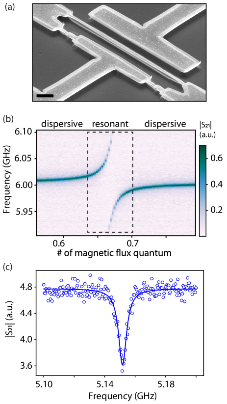
Figure 4: (a) A SEM-image of the device showing the suspended part of the SQUID loop and the Josephson junctions. The length and width of the nanowire is 40 $\mu$m and 200 nm, respectively. The scale bar corresponds to 5 $\mu$m. (b) Color plot of the cavity transmission $|S_{21}|$ as a function of the magnetic flux through the SQUID loop. (c) Two-tone measurements spectroscopic linewidth of the qubit in the dispersive regime.

After discussing the performance of the sideband cooling when the qubit is dispersively coupled to the readout cavity, we address the next question on the possibility of the mechanical readout. In the dispersive regime, there is no direct coupling between the cavity and the mechanical resonator. The modulation of qubit frequency translates to the cavity mode via dispersive coupling, and thus creating an effective coupling between the cavity and the mechanical motion. By tuning the transmon qubit frequency near half flux quantum, a large electromechanical coupling with the qubit mode can be obtained. However, when $|\omega_{q}-\omega_{c}|$ is large, the effective coupling between the cavity and mechanical mode is suppressed. Next, we show that the addition of cooling tone near the qubit frequency is helpful for the readout of the mechanical motion.

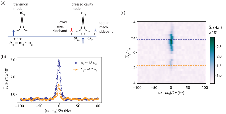
Figure 5: Experimental Data: Power spectral density of the cavity mode is measured while varying the drive detuning from the qubit mode. (a) Schematic of the measurement process. A drive is present near the qubit mode. The detuning between the qubit and the drive frequency is being changed in the measurement. A probe of frequency $\omega_{c}$ is added and its lower and upper mechanical sidebands are recorded with a spectrum analyzer. (b) The spectral density is shown for the drive detuning of $\tilde{\Delta}_{q}=-1.7~{}\omega_{m}$ and $\tilde{\Delta}_{q}=+1.7~{}\omega_{m}$. We can observe the difference in spectral height as the detuning change sign. The mechanical resonator has a frequency of $\omega_{m}/2\pi\approx$ 5.9 MHz and a linewidth $\gamma_{m}/2\pi=$ 6 Hz. (c) A colorplot of normalized spectral density as a function of detuning and measurement frequency.

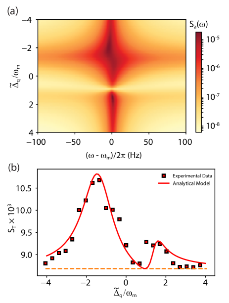
Figure 6: (a) We have evaluated the expression for the cavity mode spectrum from the theoretical model as a function of detuning $\tilde{\Delta}_{q}$ and frequency. Parameters are taken from the device studied here. (b) Plot of integrated spectrum $S_{T}=\int S_{a}(\omega)d\omega$ for different detuning is calculated from the theoretical and experimental results. The square points indicate the experimental data, plotted as a function of drive detuning ($\tilde{\Delta}_{q}$). The solid curve is plotted for estimated device parameters from analytical expression. The dashed straight line indicates noise level of the measurements. The parameters used for the plots: $\tilde{\Delta}_{c}=0$, $\omega_{m}=2\pi\times 5.9$ MHz, $J=2\pi\times 5.6$ MHz, $g=2\pi\times 3.6$ kHz, $\eta=2\pi\times 2.8$ MHz, $\kappa=2\pi\times 4$ MHz, $\Gamma=2\pi\times 8$ MHz, $\gamma_{m}=2\pi\times 6$ Hz, $n_{m}^{i}$ = 350.

For experimental realization, we use a device consisting of a transmon qubit with a doubly clamped suspended nanowire embedded in the SQUID loop. For the qubit readout, we use a 3D copper rectangular waveguide cavity. The scanning electron microscope (SEM) image of the device is shown in Fig. 4(a). The transmon, fabricated on a silicon substrate coated with highly stressed SiN, is designed to have tunable frequency realized via SQUID. One arm of the SQUID is made suspended to form a nanowire, essentially establishing the mechanical mode. The silicon substrate is placed inside the readout cavity and cool down to 20 mK in a dilution refrigerator. A detailed description of the device fabrication methods and the measurement setup can be found in Ref. [31].

Fig. 4(b) shows the cavity transmission amplitude $|S_{21}|$ as the magnetic flux through the SQUID loop is varied. When the qubit is brought in resonance with the cavity mode, the vacuum-Rabi splitting is observed and two hybrid modes emerge as indicated by the dashed box in Fig. 4(b). From the avoided-crossing, we determine the qubit-cavity coupling strength to be $75$ MHz. We measure the dressed cavity frequency to be 6.006 GHz, the maximum qubit frequency to be 7.8 GHz, and the qubit anharmonicity to be $-130$ MHz. We apply a magnetic field of $B\approx$ 1.1 mT, perpendicular to the plane of the SQUID loop. It couples the in-plane motion of the mechanical resonator to the qubit.

To operate in the dispersive limit, we choose a qubit detuning $\Delta=\omega_{q}-\omega_{c}$ of $-2\pi\times$900 MHz. A representative two-tone measurement of the qubit is shown in Fig. 4(c). To record the mechanical motion at this operating point, we apply two tones to the device, a drive tone near the qubit frequency and a probe tone near $\omega_{c}$ and record the mechanical sidebands of the probe tone using a spectrum analyzer. The positioning of various frequencies and drive tones are shown in Fig. 5(a).

Fig. 5(b) shows the recorded spectrum for two different detunings. The experimentally measured microwave spectrum $S_{mw}(\omega)$ is normalized and represented in the units of intra-cavity photons defined as, $\tilde{S}_{a}=S_{mw}(\omega)/(\hbar\omega_{c}G\kappa_{ex}RBW)$, where $G$ is the estimated net gain of the output line, $\kappa_{ex}$ is the external coupling rate of the output port of the cavity, and $RBW$ is the resolution bandwidth of the spectrum analyzer. Clearly, the spectrum has a larger peak for negative detuning as compared to the one for the positive detuning. This asymmetry becomes quite evident as the detuning of qubit drive is varied. Fig. 5(c) shows the colorplot of $\tilde{S}_{a}$ as drive frequency is varied across the qubit transition.

The mechanical resonator has a frequency of $\omega_{m}/2\pi\approx$ 5.9 MHz and a linewidth of $\gamma_{m}/2\pi\approx$ 6 Hz. Here, we do not observe any backaction on the mechanical resonator. Both, the mechanical frequency and linewidth do not show any measurable change as the detuning $\tilde{\Delta}_{q}$ is varied across the qubit frequency. This is expected behavior within the experimental parameters. For these measurements, we estimated a single-photon coupling rate of $g_{0}/2\pi\approx$ 7.5 kHz, and measured a qubit linewidth of $\Gamma/2\pi\approx$ 15 MHz. The lower sideband parameter and single-photon coupling rate reduces the effect of back-action from the qubit drive.

Another aspect of the measurement is the the enhancement of the transduction and asymmetry with respect to $\tilde{\Delta}_{q}$. Qualitatively, it can be understood from the qubit-cavity dispersive coupling and the Kerr-term of the qubit mode. A drive tone near the qubit frequency acts like a parametric pump due to the qubit-nonlinearity, resulting in the amplification of the field fluctuations due to electromechanical coupling. Further, due to the dispersive interaction between the qubit and the cavity mode, these field fluctuations result in the modulation of the intracavity probe field, and hence in an improved transduction. The asymmetry in the response is a direct manifestation of the weak anharmonicity of the qubit.

To quantitatively understand the enhancement in the transduction and the asymmetry in spectral density with respect to $\tilde{\Delta}_{q}$, we compute the cavity spectrum from Eq. 10 as a function of susceptibilities. Approximately, the cavity spectral density can be written as,

$$S_{a}(\omega) \approx n_{m}^{i}\gamma_{m}(|\chi_{m}|^{2}+|\tilde{\chi}_{m}|^{2})\sigma(\omega),\text{where}$$ (14)

$$\sigma(\omega) =\bigg{|}\frac{gJ\chi_{c}\chi_{q\tilde{q}}(\Delta_{q}-2\eta)}{\Delta_{q}+2{i}\eta^{2}\chi_{q\tilde{q}}+g^{2}\chi_{m\tilde{m}}\chi_{q\tilde{q}}(\Delta_{q}-2\eta)}\bigg{|}^{2}$$ (15)

$$\chi_{q\tilde{q}} =\chi_{q}-\tilde{\chi}_{q}$$ (16)

$$\chi_{m\tilde{m}} =\chi_{m}-\tilde{\chi}_{m}.$$ (17)

Here, we note that the presence of the effective anharmonicity $\eta$ in the above equation accounts for the asymmetry observed with respect to the detuning of qubit drive. In the limit $\eta\to 0$, the expression of $\sigma$ becomes symmetric with respect to $\Delta_{q}$ as it enters the expression through $\chi_{q\tilde{q}}$ only.

Similar to the measurement performed, we analyze the cavity spectral density as $\tilde{\Delta}_{q}$ is varied. Fig. 6(a) shows theoretically calculated $\tilde{S}_{a}(\omega)$ using the device parameters. We observe a pattern in $S_{a}(\omega)$ which is similar to the experimental measurement. For a quantitative comparison, we define the integrated spectrum as $S_{T}=\int S_{a}(\omega)d\omega$ and evaluate it for experimental data. Fig. 6(b) shows the plot of $S_{T}$ from the experimental results shown in Fig. 5(c) and theoretical calculations. A good match validates the approximation made in arriving at the effective Hamiltonian in the theoretical calculations.

VI Outlook and conclusion

To summarize, this work has investigated a coupled three-mode hybrid system with a transmon qubit in the presence of external drives. Using the quantum noise and the Lindblad formalism, we study the possibility of sideband cooling of the mechanical resonator by the qubit mode. We find that the readout of the mechanical mode is possible by coupling the transmon qubit to a readout cavity just like in standard c-QED setup while maintaining a dispersive coupling between the cavity and the qubit. In addition, we experimentally demonstrate the applicability of the readout scheme, wherein the experimental results matches closely to the analytical calculations. In this particular experiment, we do not observe any cooling of the mechanical resonator due to lower $g_{0}$ and low sideband parameter $(\omega_{m}/\Gamma\approx~{}0.4)$. While the achieved flux responsivity of the qubit in dispersive limit was high 16 GHz$/\Phi_{0}$, the estimated coupling rate ($g_{0}/2\pi\approx 7.5$ kHz) was inadequate due to the lower applied magnetic field 1.1 mT.

Looking ahead, the recent experiments have shown promising results for the transmon linewidth in the parallel magnetic field up to hundreds of mT with no significant change in the spectroscopic linewidth [42]. In addition, the flux responsivity of the qubit can be pushed to 40 GHz$/\Phi_{0}$ by increasing the maximum qubit frequency. With these parameters, the single-photon electromechanical coupling between qubit and mechanical resonator can be enhanced up to 10 MHz, bringing the system near to ultra-strong coupling regime [43]. Such regime opens up the possibilities of observing the photon blockade effects [10], non-trivial ground state [7] and a path of using low frequency mechanical resonator in the quantum technologies.

VII Acknowledgment

The authors thank G. S. Agarwal and Manas Kulkarni for valuable discussions. This material is based upon work supported by the Air Force Office of Scientific Research under award number FA2386-20-1-4003. V.S. acknowledge the support received under the Core Research Grant by the Department of Science and Technology (India). The authors acknowledge device fabrication facilities at CeNSE, IISc Bangalore, and central facilities at the Department of Physics funded by DST.

Appendix A

Spectrum of the cavity mode is calculated from Eq. 10 in the main text. In the cavity operator, it can be written as,

$$S_{a}(\omega)=\frac{1}{2\pi}\int_{-\infty}^{+\infty}\langle(\hat{a}[\omega^{\prime}])^{\dagger}\hat{a}[\omega]\rangle\mathrm{d}\omega^{\prime}.$$ (18)

Eq. 7 is used to calculate the steady state value of $\hat{a}[\omega]$, which can be written as

$$\hat{a}[\omega]=(\mathcal{B}~{}r[\omega])_{11}=\sum_{j}\mathcal{B}_{1j}(r[\omega])_{j1},$$ (19)

where $r[\omega]$ is a column matrix of noise operators of all the modes.

$$r[\omega]=\begin{bmatrix}\sqrt{\kappa_{ex}}~{}\hat{a}_{in}[\omega]+\sqrt{\kappa_{0}}~{}\hat{f}_{in}[\omega]\\ \sqrt{\kappa_{ex}}~{}(\hat{a}_{in}^{\dagger})[\omega]+\sqrt{\kappa_{0}}~{}(\hat{f}_{in}^{\dagger})[\omega]\\ \sqrt{\Gamma_{ex}}~{}\hat{c}_{in}[\omega]+\sqrt{\Gamma_{0}}~{}\hat{\xi}_{in}[\omega]\\ \sqrt{\Gamma_{ex}}~{}(\hat{c}_{in}^{\dagger})[\omega]+\sqrt{\Gamma_{0}}~{}(\hat{\xi}_{in}^{\dagger})[\omega]\\ \sqrt{\gamma_{m}}~{}\hat{b}_{in}[\omega]\\ \sqrt{\gamma_{m}}~{}(\hat{b}_{in}^{\dagger})[\omega]\end{bmatrix}$$ (20)

The noise operators in the frequency domain satisfy the following relations,

$$\langle\hat{a}_{in}[\omega](\hat{a}_{in}[\omega^{\prime}])^{\dagger}\rangle=2\pi\delta(\omega-\omega^{\prime});~{}\langle(\hat{a}_{in}[\omega])^{\dagger}\hat{a}_{in}[\omega^{\prime}]\rangle=0$$ (21a)

$$\langle\hat{f}_{in}[\omega](\hat{f}_{in}[\omega^{\prime}])^{\dagger}\rangle=2\pi\delta(\omega-\omega^{\prime});~{}\langle(\hat{f}_{in}[\omega])^{\dagger}\hat{f}_{in}[\omega^{\prime}]\rangle=0$$ (21b)

$$\langle\hat{c}_{in}[\omega](\hat{c}_{in}[\omega^{\prime}])^{\dagger}\rangle=2\pi\delta(\omega-\omega^{\prime});~{}\langle(\hat{c}_{in}[\omega])^{\dagger}\hat{c}_{in}[\omega^{\prime}]\rangle=0$$ (21c)

$$\langle\hat{\xi}_{in}[\omega](\hat{\xi}_{in}[\omega^{\prime}])^{\dagger}\rangle=2\pi\delta(\omega-\omega^{\prime});~{}\langle(\hat{\xi}_{in}[\omega])^{\dagger}\hat{\xi}_{in}[\omega^{\prime}]\rangle=0$$ (21d)

$$\langle\hat{b}_{in}[\omega](\hat{b}_{in}[\omega^{\prime}])^{\dagger}\rangle=2\pi(n_{m}^{i}+1)\delta(\omega-\omega^{\prime})$$ (21e)

$$\langle(\hat{b}_{in}[\omega])^{\dagger}\hat{b}_{in}[\omega^{\prime}]\rangle=2\pi n_{m}^{i}\delta(\omega-\omega^{\prime}),$$ (21f)

where $n_{m}^{i}$ is the thermal phonon occupancy of the mechanical mode. We can expand the Eq. 19 and write the solution of $\hat{a}[\omega]$ as,

$$\hat{a}[\omega]=\sqrt{\kappa_{ex}}\mathcal{B}_{11}[\omega]~{}\hat{a}_{in}[\omega]+\sqrt{\kappa_{0}}\mathcal{B}_{11}[\omega]~{}\hat{f}_{in}[\omega]+\sqrt{\kappa_{ex}}\mathcal{B}_{12}[\omega]~{}(\hat{a}_{in}^{\dagger})[\omega]\\ +\sqrt{\kappa_{0}}\mathcal{B}_{12}[\omega]~{}(\hat{f}_{in}^{\dagger})[\omega]+\sqrt{\Gamma_{ex}}\mathcal{B}_{13}[\omega]~{}\hat{c}_{in}[\omega]+\sqrt{\Gamma_{0}}\mathcal{B}_{13}[\omega]~{}\hat{\xi}_{in}[\omega]\\ +\sqrt{\Gamma_{ex}}\mathcal{B}_{14}[\omega]~{}(\hat{c}_{in}^{\dagger})[\omega]+\sqrt{\Gamma_{0}}\mathcal{B}_{14}[\omega]~{}(\hat{\xi}_{in}^{\dagger})[\omega]+\sqrt{\gamma_{m}}\mathcal{B}_{15}[\omega]~{}\hat{b}_{in}[\omega]\\ +\sqrt{\gamma_{m}}\mathcal{B}_{16}[\omega]~{}(\hat{b}_{in}^{\dagger})[\omega].$$ (22)

By using the identity $(x^{\dagger})[\omega]=(x[-\omega])^{\dagger}$, we can re-write the solution of $\hat{a}[\omega]$.

$$\hat{a}[\omega]=\sqrt{\kappa_{ex}}\mathcal{B}_{11}[\omega]~{}\hat{a}_{in}[\omega]+\sqrt{\kappa_{0}}\mathcal{B}_{11}[\omega]~{}\hat{f}_{in}[\omega]+\sqrt{\kappa_{ex}}\mathcal{B}_{12}[\omega]~{}(\hat{a}_{in}[-\omega])^{\dagger}\\ +\sqrt{\kappa_{0}}\mathcal{B}_{12}[\omega]~{}(\hat{f}_{in}[-\omega])^{\dagger}+\sqrt{\Gamma_{ex}}\mathcal{B}_{13}[\omega]~{}\hat{c}_{in}[\omega]+\sqrt{\Gamma_{0}}\mathcal{B}_{13}[\omega]~{}\hat{\xi}_{in}[\omega]\\ +\sqrt{\Gamma_{ex}}\mathcal{B}_{14}[\omega]~{}(\hat{c}_{in}[-\omega])^{\dagger}+\sqrt{\Gamma_{0}}\mathcal{B}_{14}[\omega]~{}(\hat{\xi}_{in}[-\omega])^{\dagger}+\sqrt{\gamma_{m}}\mathcal{B}_{15}[\omega]~{}\hat{b}_{in}[\omega]\\ +\sqrt{\gamma_{m}}\mathcal{B}_{16}[\omega]~{}(\hat{b}_{in}[-\omega])^{\dagger}.$$ (23)

From the above equation and Eq. 21f, we can calculate $\langle(\hat{a}[\omega^{\prime}])^{\dagger}\hat{a}[\omega]\rangle$,

$$\langle(\hat{a}[\omega^{\prime}])^{\dagger}\hat{a}[\omega]\rangle=2\pi\kappa_{ex}\mathcal{B}_{12}^{\ast}[\omega^{\prime}]\mathcal{B}_{12}[\omega]~{}\delta(\omega-\omega^{\prime})\\ +2\pi\kappa_{0}\mathcal{B}_{12}^{\ast}[\omega^{\prime}]\mathcal{B}_{12}[\omega]~{}\delta(\omega-\omega^{\prime})\\ +2\pi\Gamma_{ex}\mathcal{B}_{14}^{\ast}[\omega^{\prime}]\mathcal{B}_{14}[\omega]~{}\delta(\omega-\omega^{\prime})\\ +2\pi\Gamma_{0}\mathcal{B}_{14}^{\ast}[\omega^{\prime}]\mathcal{B}_{14}[\omega]~{}\delta(\omega-\omega^{\prime})\\ +2\pi n_{m}^{i}\gamma_{m}\mathcal{B}_{15}^{\ast}[\omega^{\prime}]\mathcal{B}_{15}[\omega]~{}\delta(\omega^{\prime}-\omega)\\ +2\pi(n_{m}^{i}+1)\gamma_{m}\mathcal{B}_{16}^{\ast}[\omega^{\prime}]\mathcal{B}_{16}[\omega]~{}\delta(\omega-\omega^{\prime}).$$ (24)

Substituting this to Eq. 10, the spectrum of the cavity mode can be written as,

$$S_{a}(\omega)=n_{m}^{i}\gamma_{m}(|\mathcal{B}_{15}[\omega]|^{2}+|\mathcal{B}_{16}[\omega]|^{2})+\kappa|\mathcal{B}_{12}[\omega]|^{2}+\Gamma|\mathcal{B}_{14}[\omega]|^{2}+\gamma_{m}|\mathcal{B}_{16}[\omega]|^{2},$$ (25)

where $\kappa$, $\Gamma$ and $\gamma_{m}$ are total dissipation rates of the cavity, qubit and mechanical mode respectively. $n_{m}^{i}$ is the initial mechanical mode occupancy. The terms $\mathcal{B}_{12}[\omega]$, $\mathcal{B}_{14}[\omega]$, $\mathcal{B}_{15}[\omega]$, $\mathcal{B}_{16}[\omega]$ are calculated using Wolfram Mathematica.

$$\leavevmode\resizebox{460.35788pt}{}{$\mathcal{B}_{12}[\omega]=-\frac{J^{2}\chi_{c}\tilde{\chi}_{c}(-{i}\tilde{\chi}_{q}+\chi_{q}({i}+4\eta\tilde{\chi}_{q}))}{-4{i}\eta^{2}\chi_{q}\tilde{\chi}_{q}+J^{2}(\chi_{c}-\tilde{\chi}_{c})(-{i}\tilde{\chi}_{q}+\chi_{q}({i}+4\eta\tilde{\chi}_{q}))+{i}(1+g^{2}(\chi_{q}-\tilde{\chi}_{q})(\chi_{m}-\tilde{\chi}_{m}))+4g^{2}\eta\chi_{q}\tilde{\chi}_{q}(\chi_{m}-\tilde{\chi}_{m})}$}$$ (26a)

$$\leavevmode\resizebox{460.35788pt}{}{$\mathcal{B}_{14}[\omega]=\frac{J\chi_{c}(1+2{i}\eta\chi_{q})\tilde{\chi}_{q}}{-4{i}\eta^{2}\chi_{q}\tilde{\chi}_{q}+J^{2}(\chi_{c}-\tilde{\chi}_{c})(-{i}\tilde{\chi}_{q}+\chi_{q}({i}+4\eta\tilde{\chi}_{q}))+{i}(1+g^{2}(\chi_{q}-\tilde{\chi}_{q})(\chi_{m}-\tilde{\chi}_{m}))+4g^{2}\eta\chi_{q}\tilde{\chi}_{q}(\chi_{m}-\tilde{\chi}_{m})}$}$$ (26b)

$$\leavevmode\resizebox{460.35788pt}{}{$\mathcal{B}_{15}[\omega]=-\frac{gJ\chi_{c}(-{i}\tilde{\chi}_{q}+\chi_{q}({i}+4\eta\tilde{\chi}_{q}))\chi_{m}}{-4{i}\eta^{2}\chi_{q}\tilde{\chi}_{q}+J^{2}(\chi_{c}-\tilde{\chi}_{c})(-{i}\tilde{\chi}_{q}+\chi_{q}({i}+4\eta\tilde{\chi}_{q}))+{i}(1+g^{2}(\chi_{q}-\tilde{\chi}_{q})(\chi_{m}-\tilde{\chi}_{m}))+4g^{2}\eta\chi_{q}\tilde{\chi}_{q}(\chi_{m}-\tilde{\chi}_{m})}$}$$ (26c)

$$\leavevmode\resizebox{460.35788pt}{}{$\mathcal{B}_{16}[\omega]=-\frac{gJ\chi_{c}(-{i}\tilde{\chi}_{q}+\chi_{q}({i}+4\eta\tilde{\chi}_{q}))\tilde{\chi}_{m}}{-4{i}\eta^{2}\chi_{q}\tilde{\chi}_{q}+J^{2}(\chi_{c}-\tilde{\chi}_{c})(-{i}\tilde{\chi}_{q}+\chi_{q}({i}+4\eta\tilde{\chi}_{q}))+{i}(1+g^{2}(\chi_{q}-\tilde{\chi}_{q})(\chi_{m}-\tilde{\chi}_{m}))+4g^{2}\eta\chi_{q}\tilde{\chi}_{q}(\chi_{m}-\tilde{\chi}_{m})}$}.$$ (26d)

Appendix B

From the Lindblad formalism the time-domain master equation of the density operator $\dot{\hat{\rho}}(t)$ is written as,

$$\dot{\hat{\rho}}={i}[\hat{\rho},\tilde{\mathcal{H}}]+\kappa(n_{c}^{i}+1)\mathcal{D}[\hat{a}]\hat{\rho}+\kappa n_{c}^{i}\mathcal{D}[\hat{a}^{\dagger}]\hat{\rho}+\Gamma(n_{q}^{i}+1)\mathcal{D}[\hat{c}]\hat{\rho}+\Gamma n_{q}^{i}\mathcal{D}[\hat{c}^{\dagger}]\hat{\rho}+\frac{\Gamma_{\phi}}{2}\mathcal{D}[\hat{c}^{\dagger}\hat{c}]\hat{\rho}\\ +\gamma_{m}(n_{m}^{i}+1)\mathcal{D}[\hat{b}]\hat{\rho}+\gamma_{m}n_{m}^{i}\mathcal{D}[\hat{b}^{\dagger}]\hat{\rho}.$$ (27)

Here $\kappa$ and $\gamma_{m}$ are energy relaxation rates of cavity and mechanical mode. Qubit relaxation and pure dephasing are represented as $\Gamma$ and $\Gamma_{\phi}$. The initial thermal occupancy of the cavity, qubit and the mechanical modes are $n_{c}^{i}$, $n_{q}^{i}$, and $n_{m}^{i}$ respectively. For our calculation we have considered $\Gamma_{\phi}=0$. $\mathcal{D}[\hat{\mathcal{O}}]$ is the Lindblad super-operator written as,

$$\mathcal{D}[\hat{\mathcal{O}}]\hat{\rho}:=\hat{\mathcal{O}}\hat{\rho}\hat{\mathcal{O}}^{\dagger}-\frac{1}{2}\hat{\mathcal{O}}^{\dagger}\hat{\mathcal{O}}\hat{\rho}-\frac{1}{2}\hat{\rho}\hat{\mathcal{O}}^{\dagger}\hat{\mathcal{O}}.$$ (28)

We write down the equation of motion from the Hamiltonian in Eq. (5). This is to calculate expectation values of different operators. The coupled linear equations are written in the matrix form,

$$\dot{\boldsymbol{d}}=\mathcal{M}\boldsymbol{d}+\mathcal{N},$$ (29)

where $\boldsymbol{d}$ is the column matrix consisting of the expectations values.

$$\boldsymbol{d}=\begin{bmatrix}\langle\hat{a}^{\dagger}\hat{a}\rangle\\ \langle\hat{b}^{\dagger}\hat{b}\rangle\\ \langle\hat{c}^{\dagger}\hat{c}\rangle\\ \langle\hat{a}^{2}\rangle\\ \langle\hat{a}^{\dagger 2}\rangle\\ \langle\hat{b}^{2}\rangle\\ \langle\hat{b}^{\dagger 2}\rangle\\ \langle\hat{c}\rangle\\ \langle\hat{c}^{\dagger 2}\rangle\\ \langle\hat{a}\hat{b}\rangle\\ \langle\hat{a}^{\dagger}\hat{b}^{\dagger}\rangle\\ \langle\hat{a}^{\dagger}\hat{b}\rangle\\ \langle\hat{a}\hat{b}^{\dagger}\rangle\\ \langle\hat{c}\hat{b}\rangle\\ \langle\hat{c}^{\dagger}\hat{b}^{\dagger}\rangle\\ \langle\hat{c}^{\dagger}\hat{b}\rangle\\ \langle\hat{c}\hat{b}^{\dagger}\rangle\\ \langle\hat{a}\hat{c}\rangle\\ \langle\hat{a}^{\dagger}\hat{c}^{\dagger}\rangle\\ \langle\hat{a}^{\dagger}\hat{c}\rangle\\ \langle\hat{a}\hat{c}^{\dagger}\rangle\\ \end{bmatrix}$$ (30)

$$\mathcal{M}=\leavevmode\resizebox{346.89731pt}{}{{\hbox{\setcounter{MaxMatrixCols}{21}\begin{bmatrix}-\kappa&0 &0 &0 &0 &0 &0 &0 &0 &0 &0 &0 &0 &0 &0 &0 &0 &{i}J &-{i}J &-{i}J &{i}J \\ 0 &-\gamma_{m} &0 &0 &0 &0 &0 &0 &0 &0 &0 &0 &0 &{i}g &-{i}g &{i}g &-{i}g &0 &0 &0 &0 \\ 0 &0 &-\Gamma&0 &0 &0 &0 &-2{i}\eta&2{i}\eta&0 &0 &0 &0 &{i}g &-{i}g &-{i}g &{i}g &{i}J &-{i}J &{i}J &-{i}J \\ 0 &0 &0 &1/\chi_{\hat{a}\hat{a}} &0 &0 &0 &0 &0 &0 &0 &0 &0 &0 &0 &0 &0 &-2{i}J &0 &0 &-2{i}J \\ 0 &0 &0 &0 &1/\chi_{\hat{a}\hat{a}}^{\ast} &0 &0 &0 &0 &0 &0 &0 &0 &0 &0 &0 &0 &0 &2{i}J &2{i}J &0 \\ 0 &0 &0 &0 &0 &1/\chi_{\hat{b}\hat{b}} &0 &0 &0 &0 &0 &0 &0 &-2{i}g &0 &-2{i}g &0 &0 &0 &0 &0 \\ 0 &0 &0 &0 &0 &0 &1/\chi_{\hat{b}\hat{b}}^{\ast} &0 &0 &0 &0 &0 &0 &0 &2{i}g &0 &2{i}g &0 &0 &0 &0 \\ 0 &0 &4{i}\eta&0 &0 &0 &0 &1/\chi_{\hat{c}\hat{c}} &0 &0 &0 &0 &0 &-2{i}g &0 &0 &-2{i}g &-2{i}J &0 &-2{i}J &0 \\ 0 &0 &-4{i}\eta&0 &0 &0 &0 &0 &1/\chi_{\hat{c}\hat{c}}^{\ast} &0 &0 &0 &0 &0 &2{i}g &2{i}g &0 &0 &2{i}J &0 &2{i}J \\ 0 &0 &0 &0 &0 &0 &0 &0 &0 &1/\chi_{\hat{a}\hat{b}} &0 &0 &0 &-{i}J &0 &-{i}J &0 &-{i}g &0 &0 &-{i}g \\ 0 &0 &0 &0 &0 &0 &0 &0 &0 &0 &1/\chi_{\hat{a}\hat{b}}^{\ast} &0 &0 &0 &{i}J &0 &{i}J &0 &{i}g &{i}g &0 \\ 0 &0 &0 &0 &0 &0 &0 &0 &0 &0 &0 &1/\chi_{\hat{a}^{\dagger}\hat{b}} &0 &{i}J &0 &{i}J &0 &0 &-{i}g &-{i}g &0 \\ 0 &0 &0 &0 &0 &0 &0 &0 &0 &0 &0 &0 &1/\chi_{\hat{a}^{\dagger}\hat{b}}^{\ast} &0 &-{i}J &0 &-{i}J &{i}g &0 &0 &{i}g \\ 0 &-{i}g &-{i}g &0 &0 &-{i}g &0 &-{i}g &0 &-{i}J &0 &-{i}J &0 &1/\chi_{\hat{c}\hat{b}} &0 &2{i}\eta&0 &0 &0 &0 &0 \\ 0 &{i}g &{i}g &0 &0 &0 &{i}g &0 &{i}g &0 &{i}J &0 &{i}J &0 &1/\chi_{\hat{c}\hat{b}}^{\ast} &0 &-2{i}\eta&0 &0 &0 &0 \\ 0 &{i}g &-{i}g &0 &0 &{i}g &0 &0 &-{i}g &{i}J &0 &{i}J &0 &-2{i}\eta&0 &1/\chi_{\hat{c}^{\dagger}\hat{b}} &0 &0 &0 &0 &0 \\ 0 &-{i}g &{i}g &0 &0 &0 &-{i}g &{i}g &0 &0 &-{i}J &0 &-{i}J &0 &2{i}\eta&0 &1/\chi_{\hat{c}^{\dagger}\hat{b}}^{\ast} &0 &0 &0 &0 \\ -{i}J &0 &-{i}J &-{i}J &0 &0 &0 &-{i}J &0 &-{i}g &0 &0 &-{i}g &0 &0 &0 &0 &1/\chi_{\hat{a}\hat{c}} &0 &0 &2{i}\eta\\ {i}J &0 &{i}J &0 &{i}J &0 &0 &0 &{i}J &0 &{i}g &{i}g &0 &0 &0 &0 &0 &0 &1/\chi_{\hat{a}\hat{c}}^{\ast} &-2{i}\eta&0 \\ -{i}J &0 &{i}J &0 &-{i}J &0 &0 &{i}J &0 &0 &-{i}g &-{i}g &0 &0 &0 &0 &0 &0 &2{i}\eta&1/\chi_{\hat{a}^{\dagger}\hat{c}} &0 \\ {i}J &0 &-{i}J &{i}J &0 &0 &0 &0 &-{i}J &{i}g &0 &0 &{i}g &0 &0 &0 &0 &-2{i}\eta&0 &0 &1/\chi_{\hat{a}^{\dagger}\hat{c}}^{\ast} \\ \end{bmatrix}}}}$$ (31)

Various susceptibilities are defined below.

$$\chi_{\hat{a}\hat{a}}=\frac{1}{2{i}\Delta_{c}-\kappa}$$ (32a)

$$\chi_{\hat{b}\hat{b}}=\frac{1}{-2{i}\omega_{m}-\gamma_{m}}$$ (32b)

$$\chi_{\hat{c}\hat{c}}=\frac{1}{2{i}\Delta_{q}-\Gamma-\Gamma_{\phi}}$$ (32c)

$$\chi_{\hat{a}\hat{b}}=\frac{1}{{i}(\Delta_{c}-\omega_{m})-\frac{1}{2}(\kappa+\gamma_{m})}$$ (32d)

$$\chi_{\hat{a}^{\dagger}\hat{b}}=\frac{1}{-{i}(\Delta_{c}+\omega_{m})-\frac{1}{2}(\kappa+\gamma_{m})}$$ (32e)

$$\chi_{\hat{c}\hat{b}}=\frac{1}{{i}(\Delta_{q}-\omega_{m})-\frac{1}{2}(\Gamma+\frac{\Gamma_{\phi}}{2}+\gamma_{m})}$$ (32f)

$$\chi_{\hat{c}^{\dagger}\hat{b}}=\frac{1}{-{i}(\Delta_{q}+\omega_{m})-\frac{1}{2}(\Gamma+\frac{\Gamma_{\phi}}{2}+\gamma_{m})}$$ (32g)

$$\chi_{\hat{a}\hat{c}}=\frac{1}{{i}(\Delta_{c}+\Delta_{q})-\frac{1}{2}(\Gamma+\frac{\Gamma_{\phi}}{2}+\kappa)}$$ (32h)

$$\chi_{\hat{a}^{\dagger}\hat{c}}=\frac{1}{-{i}(\Delta_{c}-\Delta_{q})-\frac{1}{2}(\Gamma+\frac{\Gamma_{\phi}}{2}+\kappa)}$$ (32i)

$$\mathcal{N}=\begin{bmatrix}n_{c}^{i}\kappa\\ n_{m}^{i}\gamma_{m}\\ n_{q}^{i}\Gamma\\ 0\\ 0\\ 0\\ 0\\ 2{i}\eta\\ -2{i}\eta\\ 0\\ 0\\ 0\\ 0\\ -{i}g\\ {i}g\\ 0\\ 0\\ -{i}J\\ {i}J\\ 0\\ 0\end{bmatrix}$$ (33)

The steady-state solution of $\boldsymbol{d}$ matrix can be written as,

$$\boldsymbol{d}=-\mathcal{M}^{-1}\mathcal{N}.$$ (34)

From Eq. 34 we have calculated the final mechanical occupation $n_{f}$ as a function of the device parameters. The plot of $n_{f}$ as a function of coupling $g$ and detuning ($\tilde{\Delta}_{q}$) is shown in Fig. 4d.

References

• Barzanjeh et al. [2022] S. Barzanjeh, A. Xuereb, S. Gröblacher, M. Paternostro, C. A. Regal, and E. M. Weig, Optomechanics for quantum technologies, Nature Physics 18, 15 (2022).
• Aspelmeyer et al. [2014] M. Aspelmeyer, T. J. Kippenberg, and F. Marquardt, Cavity optomechanics, Reviews of Modern Physics 86, 1391 (2014).
• Teufel et al. [2011] J. D. Teufel, T. Donner, D. Li, J. W. Harlow, M. S. Allman, K. Cicak, A. J. Sirois, J. D. Whittaker, K. W. Lehnert, and R. W. Simmonds, Sideband cooling of micromechanical motion to the quantum ground state, Nature 475, 359 (2011).
• Chan et al. [2011] J. Chan, T. P. M. Alegre, A. H. Safavi-Naeini, J. T. Hill, A. Krause, S. Gröblacher, M. Aspelmeyer, and O. Painter, Laser cooling of a nanomechanical oscillator into its quantum ground state, Nature 478, 89 (2011).
• Wollman et al. [2015] E. E. Wollman, C. U. Lei, A. J. Weinstein, J. Suh, A. Kronwald, F. Marquardt, A. A. Clerk, and K. C. Schwab, Quantum squeezing of motion in a mechanical resonator, Science 349, 952 (2015), .
• Ockeloen-Korppi et al. [2018] C. F. Ockeloen-Korppi, E. Damskägg, J.-M. Pirkkalainen, M. Asjad, A. A. Clerk, F. Massel, M. J. Woolley, and M. A. Sillanpää, Stabilized entanglement of massive mechanical oscillators, Nature 556, 478 (2018).
• Peterson et al. [2019] G. Peterson, S. Kotler, F. Lecocq, K. Cicak, X. Jin, R. Simmonds, J. Aumentado, and J. Teufel, Ultrastrong Parametric Coupling between a Superconducting Cavity and a Mechanical Resonator, Physical Review Letters 123, 247701 (2019).
• Kotler et al. [2021] S. Kotler, G. A. Peterson, E. Shojaee, F. Lecocq, K. Cicak, A. Kwiatkowski, S. Geller, S. Glancy, E. Knill, R. W. Simmonds, J. Aumentado, and J. D. Teufel, Direct observation of deterministic macroscopic entanglement, Science 372, 622 (2021).
• Wollack et al. [2022] E. A. Wollack, A. Y. Cleland, R. G. Gruenke, Z. Wang, P. Arrangoiz-Arriola, and A. H. Safavi-Naeini, Quantum state preparation and tomography of entangled mechanical resonators, Nature 604, 463 (2022).
• Rabl [2011] P. Rabl, Photon Blockade Effect in Optomechanical Systems, Physical Review Letters 107, 063601 (2011).
• Nunnenkamp et al. [2011] A. Nunnenkamp, K. Børkje, and S. M. Girvin, Single-Photon Optomechanics, Physical Review Letters 107, 063602 (2011).
• Rabl [2010] P. Rabl, Cooling of mechanical motion with a two-level system: The high-temperature regime, Physical Review B 82, 165320 (2010).
• Xiang et al. [2013] Z.-L. Xiang, S. Ashhab, J. Q. You, and F. Nori, Hybrid quantum circuits: Superconducting circuits interacting with other quantum systems, Reviews of Modern Physics 85, 623 (2013).
• Clerk et al. [2020] A. A. Clerk, K. W. Lehnert, P. Bertet, J. R. Petta, and Y. Nakamura, Hybrid quantum systems with circuit quantum electrodynamics, Nature Physics 16, 257 (2020).
• Martin et al. [2004] I. Martin, A. Shnirman, L. Tian, and P. Zoller, Ground-state cooling of mechanical resonators, Physical Review B 69, 125339 (2004).
• Khosla et al. [2018] K. Khosla, M. Vanner, N. Ares, and E. Laird, Displacemon Electromechanics: How to Detect Quantum Interference in a Nanomechanical Resonator, Physical Review X 8, 021052 (2018).
• Jaehne et al. [2008] K. Jaehne, K. Hammerer, and M. Wallquist, Ground-state cooling of a nanomechanical resonator via a Cooper-pair box qubit, New Journal of Physics 10, 095019 (2008).
• Hauss et al. [2008] J. Hauss, A. Fedorov, S. André, V. Brosco, C. Hutter, R. Kothari, S. Yeshwanth, A. Shnirman, and G. Schön, Dissipation in circuit quantum electrodynamics: lasing and cooling of a low-frequency oscillator, New Journal of Physics 10, 095018 (2008).
• Wang et al. [2009] Y.-D. Wang, Y. Li, F. Xue, C. Bruder, and K. Semba, Cooling a micromechanical resonator by quantum back-action from a noisy qubit, Physical Review B 80, 144508 (2009).
• Nongthombam et al. [2021] R. Nongthombam, A. Sahoo, and A. K. Sarma, Ground-state cooling of a mechanical oscillator via a hybrid electro-optomechanical system, Physical Review A 104, 023509 (2021).
• Wang et al. [2018] X. Wang, A. Miranowicz, H.-R. Li, F.-L. Li, and F. Nori, Two-color electromagnetically induced transparency via modulated coupling between a mechanical resonator and a qubit, Physical Review A 98, 023821 (2018).
• Manninen et al. [2022] J. Manninen, M. T. Haque, D. Vitali, and P. Hakonen, Enhancement of the optomechanical coupling and Kerr nonlinearity using the Josephson capacitance of a Cooper-pair box, Physical Review B 105, 144508 (2022).
• Wilson-Rae et al. [2004] I. Wilson-Rae, P. Zoller, and A. Imamoḡlu, Laser Cooling of a Nanomechanical Resonator Mode to its Quantum Ground State, Physical Review Letters 92, 075507 (2004).
• Rabl et al. [2009] P. Rabl, P. Cappellaro, M. V. G. Dutt, L. Jiang, J. R. Maze, and M. D. Lukin, Strong magnetic coupling between an electronic spin qubit and a mechanical resonator, Physical Review B 79, 041302 (2009).
• Pirkkalainen et al. [2015] J.-M. Pirkkalainen, S. U. Cho, F. Massel, J. Tuorila, T. T. Heikkilä, P. J. Hakonen, and M. A. Sillanpää, Cavity optomechanics mediated by a quantum two-level system, Nature Communications 6, 6981 (2015).
• Pirkkalainen et al. [2013] J.-M. Pirkkalainen, S. U. Cho, J. Li, G. S. Paraoanu, P. J. Hakonen, and M. A. Sillanpää, Hybrid circuit cavity quantum electrodynamics with a micromechanical resonator, Nature 494, 211 (2013).
• Viennot et al. [2018] J. Viennot, X. Ma, and K. Lehnert, Phonon-Number-Sensitive Electromechanics, Physical Review Letters 121, 183601 (2018).
• Rodrigues et al. [2019] I. C. Rodrigues, D. Bothner, and G. A. Steele, Coupling microwave photons to a mechanical resonator using quantum interference, Nature Communications 1010.1038/s41467-019-12964-2 (2019).
• Schmidt et al. [2020] P. Schmidt, M. T. Amawi, S. Pogorzalek, F. Deppe, A. Marx, R. Gross, and H. Huebl, Sideband-resolved resonator electromechanics based on a nonlinear Josephson inductance probed on the single-photon level, Communications Physics 3, 1 (2020).
• Zoepfl et al. [2020] D. Zoepfl, M. Juan, C. Schneider, and G. Kirchmair, Single-Photon Cooling in Microwave Magnetomechanics, Physical Review Letters 125, 023601 (2020).
• Bera et al. [2021] T. Bera, S. Majumder, S. K. Sahu, and V. Singh, Large flux-mediated coupling in hybrid electromechanical system with a transmon qubit, Communications Physics 410.1038/s42005-020-00514-y (2021).
• O’Connell et al. [2010] A. D. O’Connell, M. Hofheinz, M. Ansmann, R. C. Bialczak, M. Lenander, E. Lucero, M. Neeley, D. Sank, H. Wang, M. Weides, J. Wenner, J. M. Martinis, and A. N. Cleland, Quantum ground state and single-phonon control of a mechanical resonator, Nature 464, 697 (2010).
• Arrangoiz-Arriola et al. [2019] P. Arrangoiz-Arriola, E. A. Wollack, Z. Wang, M. Pechal, W. Jiang, T. P. McKenna, J. D. Witmer, R. Van Laer, and A. H. Safavi-Naeini, Resolving the energy levels of a nanomechanical oscillator, Nature 571, 537 (2019).
• Bothner et al. [2022] D. Bothner, I. C. Rodrigues, and G. A. Steele, Four-wave-cooling to the single phonon level in Kerr optomechanics, Communications Physics 5, 1 (2022).
• Luschmann et al. [2022] T. Luschmann, P. Schmidt, F. Deppe, A. Marx, A. Sanchez, R. Gross, and H. Huebl, Mechanical frequency control in inductively coupled electromechanical systems, Scientific Reports 12, 1608 (2022).
• Gambetta et al. [2006] J. Gambetta, A. Blais, D. I. Schuster, A. Wallraff, L. Frunzio, J. Majer, M. H. Devoret, S. M. Girvin, and R. J. Schoelkopf, Qubit-photon interactions in a cavity: Measurement-induced dephasing and number splitting, Physical Review A 74, 042318 (2006).
• Blais et al. [2021] A. Blais, A. L. Grimsmo, S. Girvin, and A. Wallraff, Circuit quantum electrodynamics, Reviews of Modern Physics 93, 025005 (2021).
• Zhang et al. [2005] P. Zhang, Y. D. Wang, and C. P. Sun, Cooling Mechanism for a Nanomechanical Resonator by Periodic Coupling to a Cooper Pair Box, Physical Review Letters 95, 097204 (2005).
• Kounalakis et al. [2020] M. Kounalakis, Y. M. Blanter, and G. A. Steele, Flux-mediated optomechanics with a transmon qubit in the single-photon ultrastrong-coupling regime, Physical Review Research 2, 023335 (2020).
• Gardiner and Zoller [2004] C. W. Gardiner and P. Zoller, Quantum Noise (2004).
• Lindblad [1976] G. Lindblad, On the generators of quantum dynamical semigroups, Communications in Mathematical Physics 48, 119 (1976).
• Krause et al. [2022] J. Krause, C. Dickel, E. Vaal, M. Vielmetter, J. Feng, R. Bounds, G. Catelani, J. M. Fink, and Y. Ando, Magnetic Field Resilience of Three-Dimensional Transmons with Thin-Film AlAlO${}_{\text{x}}$/Al Josephson Junctions Approaching 1 T, Physical Review Applied 17, 034032 (2022).
• Forn-Díaz et al. [2019] P. Forn-Díaz, L. Lamata, E. Rico, J. Kono, and E. Solano, Ultrastrong coupling regimes of light-matter interaction, Reviews of Modern Physics 91, 025005 (2019).