Multi-marginal Gromov–Wasserstein Transport and Barycenters

Abstract

Gromov–Wasserstein (GW) distances are combinations of Gromov–Hausdorff and Wasserstein distances that allow the comparison of two different metric measure spaces (mm-spaces). Due to their invariance under measure- and distance-preserving transformations, they are well suited for many applications in graph and shape analysis. In this paper, we introduce the concept of multi-marginal GW transport between a set of mm-spaces as well as its regularized and unbalanced versions. As a special case, we discuss multi-marginal fused variants, which combine the structure information of an mm-space with label information from an additional label space. To tackle the new formulations numerically, we consider the bi-convex relaxation of the multi-marginal GW problem, which is tight in the balanced case if the cost function is conditionally negative definite. The relaxed model can be solved by an alternating minimization, where each step can be performed by a multi-marginal Sinkhorn scheme. We show relations of our multi-marginal GW problem to (unbalanced, fused) GW barycenters and present various numerical results, which indicate the potential of the concept.

65K10, 49M20, 28A35, 28A33.

1 Introduction

Optimal transport (OT) seeks to optimally transport mass between two input measures according to some underlying cost function. Due to various applications, OT and its regularized and unbalanced variants have attracted increasing attention both from the theoretical and computational point of view in recent years [40, 45]. The metric version of OT, referred to as the Wasserstein distance, is of particular interest [56, 2]. The exact matching of the input probabilities can be relaxed, which gives rise to several distances between arbitrary measures using unbalanced OT [32, 16]. Regularized OT, which is numerically much more appealing, leads to the so-called Sinkhorn distances, which may be computed by the parallelizable Sinkhorn algorithm [19]. Associated computational aspects are treated in [15, 50]. For certain practical tasks as matching for teams [13], particle tracking [14] and information fusion [20, 21], it is useful to compute transport plans between more than two marginal measures. This is possible in the framework of multi-marginal OT [25, 39], which was tackled numerically for Coulomb costs in [7] and for repulsive costs in [18, 26]. Regularized and unbalanced variants of multi-marginal OT, which can be efficiently solved for tree-structured costs using Sinkhorn iterations, were treated in [5, 8, 27, 33]. Furthermore, the multi-marginal OT with special cost function is closely related to the OT barycenter problem, see [1, 3, 57]. The latter essentially constitute Fréchet means with respect to the OT divergence. Barycenters are of particular interest in the Wasserstein case and have been successfully applied for texture mixing [43] and Bayesian inference [48]. In an effort to reduce computational costs, slicing strategies can been leveraged to approximate (multi-marginal) OT [52, 17].

For some applications such as shape matching, a drawback of OT lies in the fact that it is not invariant to isometric transformations such as translations or rotations. A remedy are Gromov–Wasserstein (GW) distances, which were first considered by Mémoli in [35] as a modification of Gromov–Hausdorff distances and Wasserstein distances. In this framework, the objective is to match input measures living on maybe different metric spaces so that pairwise intrinsic distances are preserved. For a survey of the geometry of Gromov–Wasserstein distances, we refer to [49]. The OT literature inspired a number of generalizations for GW such as unbalanced GW distances, which were studied in [47], a sliced version of GW distances in [52, 6] and a linear one in [4]. A fused Gromov–Wasserstein distance, which also accounts for labelled input data, was introduced in [55]. A linear fused version has been discussed in [37] and a spherical sliced one in [38]. An unbalanced fused Gromov–Wasserstein distance has been used to align cortical surfaces in [51]. Furthermore, Gromov–Wasserstein distances were examined for Gaussian measures in [30, 44]. A generalization of GW distances, called co-optimal transport (COOT), was introduced in [53], and its unbalanced version was discussed in [54]. Finally, the framework of optimal tensor transport [28] provides a general formulation which encompasses OT, GW and COOT.

Similarly to the OT case, GW barycenters have gained increasing attention since their first study in [41]. Besides the computation of the measure, the GW barycenter problem also consists in the determination of the underlying metric space. To obtain a numerically tractable algorithm, Peyré, Cuturi, and Solomon [41] employ an entropic regularization of the GW distance and fix the number of support points and the measure of the barycenter beforehand. In other words, the objective is here only minimized with respect to the internal geometry of the metric space. In [59, 42], a similar procedure is used, where the entropic regularizer is replaced by a proximal term. Moreover, Brogat-Motte et al. [11] train a neural network to estimate fused GW barycenters with an a priori fixed discrete uniform distribution. A disadvantage of these methods is that the GW barycenter of two images (interpreted as probability measures) is a generic metric measure space. For applications in imaging, it would therefore be desirable to fix the geometric structure and to solely minimize with respect to the unknown measure.

The existing literature about GW distances and its applications mainly studies GW transports and matchings between two input measures. In certain applications like clustering of shapes [41, 4], multi-graph partitioning and matching [59], and graph prediction [11], a simultaneous GW-like matching of an arbitrary number of inputs is needed. So far this problem has been resolved by utilizing a reference input such as GW barycenters and using bi-marginal GW transports. An alternative approach to deal with the simultaneous matching would be to generalize the multi-marginal OT variants with respect to the GW setting.

Contributions

In this paper, inspired by multi-marginal OT, we propose a multi-marginal GW formulation which directly allows for a simultaneous matching of an arbitrary number of inputs. We also treat the associated regularized, unbalanced and fused variants. Secondly, we study the associated bi-convex relaxation and show a tightness result in the balanced setting. Thirdly, we leverage this new formulation to obtain two results regarding GW barycenters. One is mainly of theoretical nature and shows that barycenters are completely characterised by (multi-marginal) GW plans. The second result shows an unbalanced multi-marginal characterisation for barycenters with fixed support. We use the latter to obtain a novel computationally tractable algorithm for GW barycenters with possible applications in imaging and data processing.

Outline of the paper

In Section 2, we recall basic facts on GW distances. Then, in Section 3, we introduce the concept of multi-marginal GW transport. A tight relaxation of the multi-marginal GW transport is considered in Section 4. In particular, we will make use of marginal conditionally negative semi-definite kernels. The relation of multi-marginal GW transport to the GW barycenter problem is examined in Section 5. Multi-marginal fused GW transports and barycenters are studied in Section 6. Numerical proof-of-concept results in imaging are provided in Section 7.

2 Gromov–Wasserstein Distance

A metric measure space (mm-space) is a triple $\mathbb{X}\coloneqq(X,d,\mu)$ consisting of a compact metric space $(X,d)$ and a Borel probability measure $\mu$ on the Borel $\sigma$-algebra induced by the metric $d$ on $X$. Within the paper, we stick to this compact setting, although a more general treatment is possible, see e.g. [49]. In the following, we denote by $\mathcal{M}(X)$ the Banach space of signed Borel measures equipped with the total variation norm $\|\cdot\|_{\operatorname{TV}}$, by $\mathcal{M}^{+}(X)$ the subset of positive Borel measures and by $\mathcal{P}(X)$ the subset of probability measures. Recall that a sequence $(\mu_{n})_{n\in\mathbb{N}}\subset\mathcal{M}(X)$ converges weakly to $\mu\in\mathcal{M}(X)$, written $\mu_{n}\rightharpoonup\mu$, if $\int_{X}\varphi\,\,\mathrm{d}\mu_{n}(x)\to\int_{X}\varphi\,\,\mathrm{d}\mu(x)$ for all continuous functions $\varphi$ on $X$.

For the mm-spaces $\mathbb{X}_{1}\coloneqq(X_{1},d_{1},\mu_{1})$ and $\mathbb{X}_{2}\coloneqq(X_{2},d_{2},\mu_{2})$, the Gromov–Wasserstein distance is defined by

(1) $$\operatorname{GW}(\mathbb{X}_{1},\mathbb{X}_{2})\coloneqq\inf_{\pi\in\Pi(\mu_{1},\mu_{2})}\Big{(}\int_{(X_{1}\times X_{2})^{2}}\lvert d_{1}(x_{1},x_{1}^{\prime})-d_{2}(x_{2},x_{2}^{\prime})\rvert^{2}\,\mathrm{d}\pi(x_{1},x_{2})\,\mathrm{d}\pi(x_{1}^{\prime},x_{2}^{\prime})\Big{)}^{\frac{1}{2}},$$

where $\Pi(\mu_{1},\mu_{2})\subset\mathcal{P}(X_{1}\times X_{2})$ consists of all measures with marginals $\mu_{1}$ and $\mu_{2}$. By [35, Cor 10.1], the infimum in Eq. 1 is attained by some optimal GW transport plan $\pi^{*}$, which is in general not unique. Furthermore, $\operatorname{GW}(\mathbb{X}_{1},\mathbb{X}_{2})=0$ if and only if there exists a measure-preserving isometry, i.e. an isometry $\mathcal{I}\colon(X_{1},d_{1})\to(X_{2},d_{2})$ with $\mu_{2}=\mathcal{I}_{\#}\mu_{1}\coloneqq\mu_{1}\circ\mathcal{I}^{-1}$. In this case, we call $\mathbb{X}_{1}$ and $\mathbb{X}_{2}$ isomorphic to each other. The GW distance defines a metric on the quotient space of mm-spaces with respect to measure-preserving isometries [35, Thm 5.1].

Instead of fixing the marginals of the transport plan, Séjourné, Vialard, and Peyré [47] transferred the concept of unbalanced OT [32] to the GW setting by penalizing the divergences between the marginals and the given measures. To this end, recall that, for a so-called entropy function, i.e. a convex and lower semi-continuous functions $\phi\colon\mathbb{R}_{\geq 0}\to[0,\infty]$ satisfying $\phi(1)=0$, and two measures $\mu,\nu\in\mathcal{M}^{+}(X)$ with Radon–Nikodým decomposition $\mu=\,\mathrm{d}\mu/\,\mathrm{d}\nu+\mu^{\perp}$, the (Csiszár) $\phi$-divergence is given by

$$D_{\phi}(\mu,\nu)\coloneqq\int_{X}\phi\bigl{(}\tfrac{\,\mathrm{d}\mu}{\,\mathrm{d}\nu}\bigr{)}\,\mathrm{d}\nu+\phi^{\prime}_{\infty}\int_{X}\,\mathrm{d}\mu^{\perp}$$

with the convention $0\cdot\infty=0$ and the recession constant $\phi^{\prime}_{\infty}\coloneqq\lim_{x\to\infty}\phi(x)/x$. Csiszár divergences are jointly convex, weakly lower semi-continuous, and non-negative, see [32, Cor 2.9]. In this paper, we will apply the $\phi$-divergences given in Table 1.

Table 1: Entropy functions $\phi$ with recession constant $\phi_{\infty}^{\prime}$ and corresponding $\phi$-divergences.

	$\phi(t)$	$\phi_{\infty}^{\prime}$	$D_{\phi}(\mu,\nu)$
balanced ($\phi_{\mathrm{bal}}$)	$\iota_{\{1\}}(t)$	$\infty$	$\iota_{\{\nu\}}(\mu)$
unconstrained ($\phi_{\mathrm{free}}$)	$\iota_{[0,\infty)}(t)$	$0$	$0(\mu,\nu)\equiv 0$
Kullback–Leibler ($\phi_{\mathrm{BS}}$)	$t\log(t)-t+1$	$\infty$	$\operatorname{KL}(\mu,\nu)$

In particular, for the Boltzman–Shannon entropy $\phi_{\mathrm{BS}}(t)\coloneqq t\log(t)-t+1$, we obtain the Kullback–Leibler (KL) divergence

$$\operatorname{KL}(\mu,\nu)\coloneqq\begin{cases}\int\log\bigl{(}\frac{\,\mathrm{d}\mu}{\,\mathrm{d}\nu}\bigr{)}\,\mathrm{d}\nu-\mu(X)+\nu(X),&\mu\ll\nu,\\ \infty,&\text{else}.\end{cases}$$

The regularized, unbalanced GW transport [47] is given for $\varepsilon\geq 0$ by

$$\operatorname{UGW}_{\varepsilon}(\mathbb{X}_{1},\mathbb{X}_{2})\coloneqq\!\!\!\!\!\inf_{\pi\in\mathcal{M}^{+}(X_{1}\times X_{2})}\Big{(}\int_{(X_{1}\times X_{2})^{2}}\!\!\!\!\!|d_{1}-d_{2}|^{2}\,\mathrm{d}\pi\,\mathrm{d}\pi+\sum_{i=1}^{2}D_{\phi_{i}}^{\otimes}(\pi_{i},\mu_{i})+\varepsilon\operatorname{KL}^{\otimes}(\pi,\mu_{1}\otimes\mu_{2})\Big{)}^{\frac{1}{2}}$$

with $D_{\phi_{i}}^{\otimes}(\mu,\nu)\coloneqq D_{\phi_{i}}(\mu\otimes\mu,\nu\otimes\nu)$, $\operatorname{KL}^{\otimes}\coloneqq D_{\phi_{\text{BS}}}^{\otimes}$, and marginals $\pi_{i}\coloneqq(P_{i})_{\#}\pi$, where $P_{i}(x_{1},x_{2})\coloneqq x_{i}$, $i=1,2$. We use similar notations for projections onto the components of higher-order Cartesian products. Depending on the chosen divergence, the marginals of the computed plan may match the given $\mu_{i}$ (balanced), be close to them (scaled Kullback–Leibler), or completely free (unconstrained). In the unbalanced setting, the given $\mu_{i}$ do not have to be probability measures, i.e. $\mu_{i}\in\mathcal{M}^{+}(X_{i})$. To keep the notation simple, we use $\mu_{1}\otimes\mu_{2}$ in the KL regularization. However, this could be replaced by the the product of Lebesgue measures or counting measures on the respective spaces, see [5, 36].

3 Multi-marginal Gromov–Wasserstein Transport

Towards a multi-marginal GW setting, we consider a series of mm-spaces $\mathbb{X}_{i}\coloneqq(X_{i},d_{i},\mu_{i})$, $i=1,\dots,N$. The Cartesian product of the domains is henceforth denoted by

$$\bm{X}\coloneqq\bigtimes_{i=1}^{N}X_{i}\qquad\text{with}\qquad\bm{x}\coloneqq(x_{1},\dots,x_{N}),\;x_{i}\in X_{i}.$$

We introduce the multi-marginal GW transport problem as

$$\operatorname{MGW}(\mathbb{X}_{1},\dotsc,\mathbb{X}_{N})\coloneqq\inf_{\pi\in\Pi(\mu_{1},\dots,\mu_{N})}\int_{\bm{X}^{2}}c(\bm{x},\bm{x}^{\prime})\,\mathrm{d}\pi(\bm{x})\,\mathrm{d}\pi(\bm{x}^{\prime}),$$

where $\Pi(\mu_{1},\dots,\mu_{N})\coloneqq\{\pi\in\mathcal{P}(X):(P_{i})_{\#}\pi=\mu_{i}\}$ and $c\colon\bm{X}\times\bm{X}\to[0,\infty]$ is dependent on $d_{1},\dotsc,d_{N}$. A typical cost function is

(2) $$c(\bm{x},\bm{x}^{\prime})\coloneqq\sum_{i,j=1}^{N}c_{ij}|d_{i}(x_{i},x^{\prime}_{i})-d_{j}(x_{j},x_{j}^{\prime})|^{2}\qquad\text{with}\qquad c_{ij}\geq 0.$$

In analogy to the unbalanced GW transport, we consider for $\varepsilon\geq 0$, the regularized, unbalanced multi-marginal GW transport problem

$$\operatorname{UMGW}_{\varepsilon}(\mathbb{X}_{1},\dotsc,\mathbb{X}_{N})\coloneqq\inf_{\pi\in\mathcal{M}^{+}(\bm{X})}F_{\varepsilon}(\pi)$$

$$F_{\varepsilon}(\pi)\coloneqq\int_{\bm{X}^{2}}c(\bm{x},\bm{x}^{\prime})\,\mathrm{d}\pi(\bm{x})\,\mathrm{d}\pi(\bm{x}^{\prime})+\sum_{i=1}^{N}D_{\phi_{i}}^{\otimes}(\pi_{i},\mu_{i})+\varepsilon\operatorname{KL}^{\otimes}(\pi,\mu^{\otimes}),$$

where $\mu^{\otimes}\coloneqq\mu_{1}\otimes\cdots\otimes\mu_{N}$. Under mild conditions, the infimum is attained.

Proposition 3.1 (Existence of Minimizer).

Let the cost function $c\colon\bm{X}\times\bm{X}\to\mathbb{R}_{+}$ be lower semi-continuous. Assume either $\varepsilon>0$ or $\sum_{i=1}^{N}(\phi_{i})^{\prime}_{\infty}>0$. Then $\operatorname{UMGW}_{\varepsilon}$ is finite and the infimum is attained.

The statement can be shown by following the lines in the proof of [47, Prop 7]. To make the paper self-contained, we give the proof in the appendix.

4 Bi-convex Relaxation

In this section, we consider a bi-convex relaxation of $\operatorname{UMGW}_{\varepsilon}$. If the cost function belongs to a certain class of conditionally negative definite functions, then we will see that the relaxation of the balanced problem becomes tight, that is, the values and minimizers of the original problem and the relaxed problem coincide. We introduce this class of cost functions, before we deal with the bi-convex relaxation.

4.1 Conditionally Negative Semi-definiteness

In the following, we consider the results from [53, 34] from a multi-marginal point of view. Recall that a symmetric matrix $A\in\mathbb{R}^{d\times d}$ is negative semi-definite if $\alpha^{\mathrm{T}}A\alpha\leq 0$ for all $\alpha\coloneqq(\alpha(i))_{i=1}^{d}\in\mathbb{R}^{d}$. This is equivalent to the fact that $A$ has only non-positive eigenvalues. Furthermore, $A\in\mathbb{R}^{d\times d}$ is conditionally negative semi-definite on a subspace $V\subset\mathbb{R}^{d}$ if $v^{\mathrm{T}}Av\leq 0$ for all $v\in V$. If the columns of $B\in\mathbb{R}^{d\times\dim V}$ form an orthonormal basis of $V$, this is equivalent to $\alpha^{\mathrm{T}}B^{\mathrm{T}}AB\alpha\leq 0$ for all $\alpha\in\mathbb{R}^{\dim V}$, i.e. to the negative semi-definiteness of $B^{\mathrm{T}}AB\in\mathbb{R}^{\dim V\times\dim V}$.

A continuous, symmetric function $k\colon X\times X\rightarrow\mathbb{R}$ is negative definite, if for all points $x^{1},\ldots,x^{d}\in X$ and all $d\in\mathbb{N}$, the matrix $\left(k(x^{m},x^{n})\right)_{m,n=1}^{d}$ is negative semi-definite. It is called conditionally negative definite (of order 1) if this holds true on the subspace

$$V_{{\bf 1}_{d}}\coloneqq\{\alpha\coloneqq(\alpha(j))_{j=1}^{d}\in\mathbb{R}^{d}:\alpha^{\mathrm{T}}\mathbf{1}_{d}=0\},$$

see [46, 58]. Equivalently, the above function $k\colon X\times X\to\mathbb{R}$ is conditionally negative definite if

$$\sum_{m,n=1}^{d}k(x^{m},x^{n})\,\alpha(x^{m})\alpha(x^{n})\leq 0$$

for all $\mathcal{X}\coloneqq\{x^{m}\in X:m=1,\ldots,d\}$, $d\in\mathbb{N}$, and for all $\alpha\in\mathcal{M}(\mathcal{X})$ satisfying $\alpha(\mathcal{X})=0$. Typical conditionally negative definite functions are the Euclidean metric $\|x-y\|_{2}$ on $\mathbb{R}^{d}$ and spherical distances $d(x,y)$, see [10]. For further examples, we refer to [22]. We will need the following auxiliary lemma.

Lemma 4.1.

Let $A_{i}\in\mathbb{R}^{d_{i}\times d_{i}}$ be symmetric, and let $V_{i}\subset\mathbb{R}^{d_{i}}$, $i=1,2$, be subspaces. Then $-(A_{1}\otimes A_{2})$ is conditionally negative semi-definite on $V_{1}\otimes V_{2}$ if and only if either $A_{i}$, $i=1,2$, or $-A_{i}$, $i=1,2$, are conditionally negative semi-definite on $V_{i}$, $i=1,2$.

Proof 4.2.

Let $B_{i}\in\mathbb{R}^{d_{i}\times\dim V_{i}}$ be matrices whose columns form an orthonormal bases of $V_{i}$, $i=1,2$. Then $B_{1}\otimes B_{2}$ is a basis of $V_{1}\otimes V_{2}$ and $-(A_{1}\otimes A_{2})$ is conditionally negative semi-definite on $V_{1}\otimes V_{2}$ if and only if

$$-(B_{1}\otimes B_{2})^{\mathrm{T}}(A_{1}\otimes A_{2})(B_{1}\otimes B_{2})=-(B_{1}^{\mathrm{T}}A_{1}B_{1})\otimes(B_{2}^{\mathrm{T}}A_{2}B_{2})$$

is negative semi-definite. Considering that the eigenvalues on the right-hand side are the negative pairwise products of the eigenvalues of $B_{i}^{\mathrm{T}}A_{i}B_{i}$, $i=1,2$, we obtain the assertion.

In our application, the cost function is given on the compact Cartesian space $\bm{X}\coloneqq\bigtimes_{i=1}^{N}X_{i}$, $N\geq 2$ and often has a special structure as the one in Eq. 2. This gives rise to the following definition. For $M\coloneqq(M_{i})_{i=1}^{N}\in\mathbb{N}^{N}$, let $[M]\coloneqq\{m=(m_{1},\ldots,m_{N})\in\mathbb{N}^{N}:1\leq m_{i}\leq M_{i}\}$. A continuous, symmetric function $c\colon\bm{X}\times\bm{X}\to\mathbb{R}$ is called marginal conditionally negative definite if

(3) $$\sum_{m,n\in[M]}c(\bm{x}^{m},\bm{x}^{n})\,\alpha(\bm{x}^{m})\alpha(\bm{x}^{n})\leq 0,\qquad\bm{x}^{m}\coloneqq\left(x_{1}^{m_{1}},\ldots,x_{N}^{m_{N}}\right)\in\bigtimes_{i=1}^{N}\mathcal{X}_{i},$$

for all $\mathcal{X}_{i}\coloneqq\{x_{i}^{m_{i}}\in X_{i}:m_{i}=1,\ldots,M_{i}\}$, $M\in\mathbb{N}^{N}$ and for all $\alpha\in\mathcal{M}(\bigtimes{\!}_{i=1}^{N}\mathcal{X}_{i})$ satisfying $(P_{i})_{\#}\alpha\equiv 0$ for $1\leq i\leq N$. Clearly, a conditionally negative definite function is marginal conditionally negative definite, but not conversely. Then we have the following proposition.

Proposition 4.3.

Let $c\colon\bm{X}\times\bm{X}\to\mathbb{R}$ be defined by Eq. 2, where $d_{i}$, $i=1,\dots,N$, are conditionally negative semi-definite functions. Then $c$ is marginal conditionally negative definite.

Proof 4.4.

Since the sum of marginal conditionally negative definite functions keeps this property, it remains to restrict our attention to the function

$$|d_{i}(x_{i},x_{i}^{\prime})-d_{j}(x_{j},x_{j}^{\prime})|^{2}=d_{i}^{2}(x_{i},x_{i}^{\prime})+d_{j}^{2}(x_{j},x_{j}^{\prime})-2d_{i}(x_{i},x_{i}^{\prime})d_{j}(x_{j},x_{j}^{\prime}).$$

By definition of $\alpha$, we have that

$$\sum_{m,n\in[M]}d_{i}^{2}(x_{i}^{m_{i}},x_{i}^{n_{i}})\,\alpha(\bm{x}^{m})\alpha(\bm{x}^{n})=\sum_{m_{i},n_{i}}d_{i}^{2}(x_{i}^{m_{i}},x_{i}^{n_{i}})\,\bigl{[}(P_{i})_{\#}\alpha\bigr{]}(x_{i}^{m_{i}})\,\bigl{[}(P_{i})_{\#}\alpha\bigr{]}(x_{i}^{n_{i}})=0$$

and that $-d_{i}(x_{i},x_{i}^{\prime})d_{j}(x_{j},x_{j}^{\prime})$ is negative semi-definite on $\bm{X}\times\bm{X}$ if and only if this is true on $(X_{i}\times X_{j})\times(X_{i}\times X_{j})$. For the latter, it remains to show that $-(d_{i}(x_{i}^{m_{i}},x_{i}^{n_{i}}))_{m_{i},n_{i}=1}^{M_{i}}\otimes(d_{j}(x_{j}^{m_{j}},x_{j}^{n_{j}}))_{m_{j},n_{j}=1}^{M_{j}}$ is negative semi-definite on $V_{{\bf 1}_{M_{i}}}\otimes V_{{\bf 1}_{M_{j}}}$. By Lemma 4.1 this is indeed the case.

4.2 Tight Bi-convex Relaxation

The objective $F_{\varepsilon}$ in $\operatorname{UMGW}_{\varepsilon}$ is quadratic in $\pi$. Inspired from [47] for GW distances, we propose the following bi-convex relaxation to tackle $\operatorname{UMGW}_{\varepsilon}$ numerically:

$$\operatorname{UMGW}_{\varepsilon}^{\mathrm{bi}}(\mathbb{X}_{1},\dotsc,\mathbb{X}_{N})\coloneqq\inf_{\pi,\gamma\in\mathcal{M}^{+}(\bm{X})}F^{\mathrm{bi}}_{\varepsilon}(\pi,\gamma)$$

$$F^{\mathrm{bi}}_{\varepsilon}(\pi,\gamma)\coloneqq\int_{\bm{X}^{2}}c(\bm{x},\bm{x}^{\prime})\,\mathrm{d}\pi(\bm{x})\,\mathrm{d}\gamma(\bm{x}^{\prime})+\sum_{i=1}^{N}D_{\phi_{i}}(\pi_{i}\otimes\gamma_{i},\mu_{i}\otimes\mu_{i})+\varepsilon\operatorname{KL}\bigl{(}\pi\otimes\gamma,(\mu^{\otimes})^{2}\bigr{)}.$$

By construction, the relaxation always satisfies $\operatorname{UMGW}_{\varepsilon}^{\mathrm{bi}}\leq\operatorname{UMGW}_{\varepsilon}$. Moreover, in the balanced case, it becomes tight for marginal conditionally negative definite cost functions, meaning that any minimizer $(\pi^{*},\gamma^{*})$ of $\operatorname{UMGW}_{\varepsilon}^{\mathrm{bi}}$ yields the minimizers $\pi^{*}$ and $\gamma^{*}$ of $\operatorname{UMGW}_{\varepsilon}$.

Proposition 4.5 (Tightness of Relaxation).

Let $\phi_{i}\coloneqq\phi_{\mathrm{bal}}$, $i=1,\ldots,N$, $\varepsilon\geq 0$ and $c$ be marginal conditionally negative definite. Then, $\operatorname{UMGW}_{\varepsilon}=\operatorname{UMGW}_{\varepsilon}^{\mathrm{bi}}$ and every minimizer $(\pi^{*},\gamma^{*})$ of $\operatorname{UMGW}_{\varepsilon}^{\mathrm{bi}}$ satisfies

(4) $$F_{\varepsilon}^{\mathrm{bi}}(\pi^{*},\gamma^{*})=F_{\varepsilon}^{\mathrm{bi}}(\pi^{*},\pi^{*})=F_{\varepsilon}^{\mathrm{bi}}(\gamma^{*},\gamma^{*})$$

such that $\pi^{*}$ and $\gamma^{*}$ are minimizers of $\operatorname{UMGW}_{\varepsilon}$.

Proof 4.6.

The balanced setting ensures that all occurring measures are probability measures. The KL divergence then splits into $\operatorname{KL}(\pi\otimes\gamma,\mu^{\otimes}\otimes\mu^{\otimes})=\operatorname{KL}(\pi,\mu^{\otimes})+\operatorname{KL}(\gamma,\mu^{\otimes})$ by [47, Prop 9]. Furthermore, the values in Eq. 4 always satisfy

$$F_{\varepsilon}^{\mathrm{bi}}(\pi^{*},\gamma^{*})\leq F_{\varepsilon}^{\mathrm{bi}}(\pi^{*},\pi^{*})\qquad\text{and}\qquad F_{\varepsilon}^{\mathrm{bi}}(\pi^{*},\gamma^{*})\leq F_{\varepsilon}^{\mathrm{bi}}(\gamma^{*},\gamma^{*})$$

Incorporating the KL splitting, and defining $K(\pi,\gamma)\coloneqq\int_{\bm{X}^{2}}c\,\mathrm{d}\pi\,\mathrm{d}\gamma$, we obtain

(5) $$K(\pi^{*},\gamma^{*})+\varepsilon\operatorname{KL}(\pi^{*},\mu^{\otimes})+\varepsilon\operatorname{KL}(\gamma^{*},\mu^{\otimes}) \leq K(\pi^{*},\pi^{*})+2\varepsilon\operatorname{KL}(\pi^{*},\mu^{\otimes}),$$

(6) $$K(\pi^{*},\gamma^{*})+\varepsilon\operatorname{KL}(\pi^{*},\mu^{\otimes})+\varepsilon\operatorname{KL}(\gamma^{*},\mu^{\otimes}) \leq K(\gamma^{*},\gamma^{*})+2\varepsilon\operatorname{KL}(\gamma^{*},\mu^{\otimes}).$$

Now, assume that Eq. 4 is false, i.e. at least one of the inequalities Eqs. 5 and 6 is strict. Summing both inequalities then yields

(7) $$0<K(\pi^{*}-\gamma^{*},\pi^{*}-\gamma^{*})=K(\alpha,\alpha)\qquad\text{with}\qquad\alpha\coloneqq\pi^{*}-\gamma^{*}.$$

Since $\pi^{*},\gamma^{*}\in\Pi(\mu_{1},\dots,\mu_{N})$, we have $(P_{i})_{\#}\alpha\equiv 0$, $i=1,\ldots,N$. Then the marginal conditionally negative definiteness of $c$ ensures $K(\alpha,\alpha)\leq 0$. This is however a contradiction to Eq. 7.

Note that the proposition does not immediately follow from [47, Thm 2] since the proof given there is not reproducible in the non-definite case. More precisely, $x^{\mathrm{T}}Ax=0$, $x^{\mathrm{T}}\bf 1=0$ does not imply $x\in\text{ker}A$ for a conditionally negative semi-definite matrix $A$.

The bi-convex relaxation $\operatorname{UMGW}_{\varepsilon}$ encourages to use an alternating minimization scheme over $\pi$ and $\gamma$. Here the minimization over one variable corresponds to a multi-marginal optimal transport problem with a specific cost function. In the following proposition, we restrict our attention to the divergences from Table 1.

Proposition 4.7.

Let $\phi_{i}$, $i=1,\dotsc,N$, be an entropy function from Table 1, and set $\mathcal{I}\coloneqq\{i:\phi_{i}=\phi_{\mathrm{BS}}\}$. Then, for fixed $\gamma\in\mathcal{M}^{+}(X)$ with $D_{\phi_{i}}(\gamma_{i},\mu_{i})<\infty$ and $\operatorname{KL}(\gamma,\mu)<\infty$, the minimization over $\pi$ in $\operatorname{UMGW}_{\varepsilon}^{\mathrm{bi}}$ becomes the multi-marginal transport problem

$$\operatorname*{argmin}_{\pi\in\mathcal{M}^{+}(\bm{X})}F^{\mathrm{bi}}_{\varepsilon}(\pi,\gamma)\coloneqq\int_{X}c_{\gamma}(\bm{x})\,\mathrm{d}\pi(\bm{x})+\|\gamma\|_{\operatorname{TV}}\,\Bigl{(}\sum_{i=1}^{N}D_{\phi_{i}}(\pi_{i},\mu_{i})\Bigr{)}+\varepsilon\|\gamma\|_{\operatorname{TV}}\operatorname{KL}(\pi,\mu^{\otimes})$$

with

(8) $$c_{\gamma}(\bm{x})\coloneqq\int_{\bm{X}}c(\bm{x},\bm{x}^{\prime})\,\mathrm{d}\gamma(\bm{x}^{\prime})+\Bigl{[}\sum_{i\in\mathcal{I}}\int_{X_{i}}\log\bigl{(}\tfrac{\,\mathrm{d}\gamma_{i}}{\,\mathrm{d}\mu_{i}}\bigr{)}\,\mathrm{d}\gamma_{i}\Bigr{]}+\varepsilon\int_{\bm{X}}\log\bigl{(}\tfrac{\,\mathrm{d}\gamma}{\,\mathrm{d}\mu^{\otimes}}\bigr{)}\,\mathrm{d}\gamma.$$

Proof 4.8.

For arbitrary measures $\alpha_{1}$, $\alpha_{2}$, $\alpha_{3}\in\mathcal{M}^{+}(Y)$, the KL divergence factorizes into

$$\operatorname{KL}(\alpha_{1}\otimes\alpha_{2},\alpha_{3}\otimes\alpha_{3}) =\|\alpha_{1}\|_{\operatorname{TV}}\,\operatorname{KL}(\alpha_{2},\alpha_{3})+\|\alpha_{2}\|_{\operatorname{TV}}\,\operatorname{KL}(\alpha_{1},\alpha_{3})$$

$$\qquad+(\|\alpha_{1}\|_{\operatorname{TV}}-\|\alpha_{3}\|_{\operatorname{TV}})\,(\|\alpha_{2}\|_{\operatorname{TV}}-\|\alpha_{3}\|_{\operatorname{TV}}),$$

see [47, Prop 9]. Using the definition of Csiszár divergences, we especially have

(9) $$\operatorname{KL}(\alpha_{1}\otimes\alpha_{2},\alpha_{3}\otimes\alpha_{3}) =\|\alpha_{1}\|_{\operatorname{TV}}\,\int_{Y}\log(\tfrac{\,\mathrm{d}\alpha_{2}}{\,\mathrm{d}\alpha_{3}})\,\mathrm{d}\alpha_{2}+\|\alpha_{2}\|_{\operatorname{TV}}\,\operatorname{KL}(\alpha_{1},\alpha_{3})$$

$$\qquad-\|\alpha_{3}\|_{\operatorname{TV}}\,(\|\alpha_{2}\|_{\operatorname{TV}}-\|\alpha_{3}\|_{\operatorname{TV}}).$$

Assume $D_{\phi}(\alpha_{2},\alpha_{3})<\infty$, we can factorize the balanced and unconstrained divergences into

(10) $$\iota_{\{\alpha_{3}\otimes\alpha_{3}\}}(\alpha_{1}\otimes\alpha_{2}) =\|\alpha_{1}\|_{\operatorname{TV}}\,\iota_{\{\alpha_{3}\}}(\alpha_{2})+\|\alpha_{2}\|_{\operatorname{TV}}\,\iota_{\{\alpha_{3}\}}(\alpha_{1})=\|\alpha_{2}\|_{\operatorname{TV}}\,\iota_{\{\alpha_{3}\}}(\alpha_{1})$$

(11) $$0(\alpha_{1}\otimes\alpha_{2},\alpha_{3}\otimes\alpha_{3}) =\|\alpha_{1}\|_{\operatorname{TV}}\,0(\alpha_{2},\alpha_{3})+\|\alpha_{2}\|_{\operatorname{TV}}\,0(\alpha_{1},\alpha_{3})=\|\alpha_{2}\|_{\operatorname{TV}}\,0(\alpha_{1},\alpha_{3}).$$

Applying Eqs. 9, 10, and 11, and exploiting $D_{\phi_{i}}(\gamma_{i},\mu_{i})<\infty$ and $\operatorname{KL}(\gamma,\mu)<\infty$, we have

$$F_{\varepsilon}^{\mathrm{bi}}(\pi,\gamma) =\int_{\bm{X}^{2}}c(\bm{x},\bm{x}^{\prime})\,\mathrm{d}\pi(\bm{x})\,\mathrm{d}\gamma(\bm{x}^{\prime})+\sum_{i\not\in\mathcal{I}}\|\gamma_{i}\|_{\operatorname{TV}}\,D_{\phi_{i}}(\pi_{i},\mu_{i})$$

$$\;+\sum_{i\in\mathcal{I}}\Bigl{(}\int_{\bm{X}}\int_{X_{i}}\log\bigl{(}\tfrac{\,\mathrm{d}\gamma_{i}}{\,\mathrm{d}\mu_{i}}\bigr{)}\,\mathrm{d}\gamma_{i}\,\mathrm{d}\pi+\|\gamma_{i}\|_{\operatorname{TV}}\,\operatorname{KL}(\pi_{i},\mu_{i})+\underbrace{\|\mu_{i}\|_{\operatorname{TV}}^{2}-\|\gamma_{i}\|_{\operatorname{TV}}\,\|\mu_{i}\|_{\operatorname{TV}}}_{\text{constant}}\Bigr{)}$$

$$\;+\varepsilon\,\Bigl{(}\int_{\bm{X}}\int_{\bm{X}}\log\bigl{(}\tfrac{\,\mathrm{d}\gamma}{\,\mathrm{d}\mu^{\otimes}}\bigr{)}\,\mathrm{d}\gamma\,\mathrm{d}\pi+\|\gamma\|_{\operatorname{TV}}\,\operatorname{KL}(\pi,\mu^{\otimes})+\underbrace{\|\mu^{\otimes}\|_{\operatorname{TV}}^{2}-\|\gamma\|_{\operatorname{TV}}\,\|\mu^{\otimes}\|_{\operatorname{TV}}}_{\text{constant}}\Bigr{)}.$$

Rearranging terms and omitting the constant terms yields the assertion.

The minimization of $F^{\mathrm{bi}}_{\varepsilon}(\cdot,\gamma)$ over $\mathcal{M}^{+}(\bm{X})$ may be efficiently solved using the multi-marginal Sinkhorn scheme in [5] if the cost function has a sparse structure. For example, we can use cost functions of the form Eq. 2 with $N-1$ non-zero coefficients $c_{ij}$ such that Eq. 2 decouples according to a tree, that is, there is no sequence $i_{1},\dotsc,i_{k}$ with $c_{i_{1},i_{2}},\dotsc,c_{i_{k-1},i_{k}}>0$ and $i_{1}=i_{k}$. Similarly to [47, Alg 1], the bi-convex relaxation leads to the alternating minimization scheme in Algorithm 1. Since $F_{\varepsilon}^{\mathrm{bi}}$ is invariant under $(\pi,\gamma)\mapsto(t\,\pi,\frac{1}{t}\,\gamma)$ for $t>0$, the measures may be balanced such that $\|\pi\|_{\operatorname{TV}}=\|\gamma\|_{\operatorname{TV}}$. In the algorithm, the rescaling of the newly computed variable corresponds this balancing. The algorithm produces a sequence $\pi_{1},\gamma_{1},\pi_{2},\gamma_{2},\dots$ which monotonously decreases the lower-bounded objective $F^{\mathrm{bi}}_{\varepsilon}$. Hence, the sequence $(F^{\mathrm{bi}}_{\varepsilon}(\pi_{k},\gamma_{k}))_{k\in\mathbb{N}}$ converges. However, in general it may happen that $(\pi_{k},\gamma_{k})_{k\in\mathbb{N}}$ do not converge. Even if the iterates converge, i.e. $\pi_{k}\to\pi$, $\gamma_{k}\to\gamma$, the limits may not coincide. However, in our numerical experiments, we usually observe convergence to a single limit $\pi=\gamma$.

Input: mm-spaces $\mathbb{X}_{i}\coloneqq(X_{i},d_{i},\mu_{i})$, $i=1,\dots,N$; cost function $c$; entropy functions $\varphi_{i}$, $i=1,\dots,N$, from Table 1; regularization parameter $\varepsilon>0$.

Initialize $\pi\coloneqq\gamma\coloneqq\bigotimes_{i=1}^{N}\mu_{i}$.

while not converged do

     Compute $c_{\gamma}$ in Eq. 8.

     Update $\pi$ using the Sinkhorn scheme in [5] with $c_{\gamma}$.

     Rescale by $\pi\leftarrow\sqrt{\|\gamma\|_{\operatorname{TV}}/\|\pi\|_{\operatorname{TV}}}\,\pi$.

     Compute $c_{\pi}$ in Eq. 8.

     Update $\gamma$ using the Sinkhorn scheme in [5] with $c_{\pi}$.

     Rescale by $\gamma\leftarrow\sqrt{\|\pi\|_{\operatorname{TV}}/\|\gamma\|_{\operatorname{TV}}}\,\gamma$.

end while

Output: $(\gamma,\pi)$

Algorithm 1 (Unbalanced) Multi-marginal Gromov–Wasserstein Transport

5 Barycenters

Barycenters and multi-marginal optimal transport problems are closely related [3, 5, 13, 27]. For the GW setting, we obtain similar results. For $\rho_{i}\geq 0$ with $\sum_{i=1}^{N}\rho_{i}=1$, a Gromov–Wasserstein barycenter between the mm-spaces $\mathbb{X}_{i}\coloneqq(X_{i},d_{i},\mu_{i})$, $i=1,\dots,N$, is a minimizing mm-space $\mathbb{Y}\coloneqq(Y,d,\nu)$ of

(12) $$\inf_{\mathbb{Y}}\sum_{i=1}^{N}\rho_{i}\operatorname{GW}^{2}(\mathbb{X}_{i},\mathbb{Y}).$$

Indeed the next result shows that solutions always exist and characterizes them via multi-marginal solutions.

Theorem 5.1 (Free-Support Barycenter).

Let $\mathbb{X}_{i}$ be given mm-spaces, and let $\rho_{i}\geq 0$ be weights with $\sum_{i=1}^{N}\rho_{i}=1$. Then the infimum in Eq. 12 is attained. Moreover, each solution of Eq. 12 is isomorphic to an mm-space of the form $\mathbb{Y}^{*}\coloneqq(\bm{X},d^{*},\pi^{*})$, where $d^{*}(\bm{x},\bm{x}^{\prime})\coloneqq\sum_{i=1}^{N}\rho_{i}d_{i}(x_{i},x_{i}^{\prime})$, and $\pi^{*}$ is a minimizer of $\operatorname{MGW}(\mathbb{X}_{1},\dots,\mathbb{X}_{N})$ with cost function

$$c(\bm{x},\bm{x}^{\prime})\coloneqq\frac{1}{2}\sum_{i,j=1}^{N}\rho_{i}\rho_{j}\,\lvert d_{i}(x_{i},x_{i}^{\prime})-d_{j}(x_{j},x_{j}^{\prime})\rvert^{2}.$$

Proof 5.2.

First we note that the cost function may be rearranged as

$$c(\bm{x},\bm{x}^{\prime})=\sum_{i=1}^{N}\rho_{i}\,d_{i}^{2}(x_{i},x_{i}^{\prime})-\sum_{i,j=1}^{N}\rho_{i}\rho_{j}\,d_{i}(x_{i},x_{i}^{\prime})\,d_{j}(x_{j},x_{j}^{\prime})=\sum_{i=1}^{N}\rho_{i}\,\Bigl{|}d_{i}(x_{i},x_{i}^{\prime})-\overbrace{\sum_{j=1}^{N}\rho_{j}\,d_{j}(x_{j},x_{j}^{\prime})}^{=d^{*}(x,x^{\prime})}\Bigr{|}^{2}.$$

Let $\mathbb{Y}=(Y,d,\nu)$ be an arbitrary mm-space, and let $\pi^{(i)}_{\operatorname{GW}}$ be an optimal plan of $\operatorname{GW}(\mathbb{X}_{i},\mathbb{Y})$, $i=1,\dotsc,N$. Since all these plans have the marginal $(P_{2})_{\#}\pi^{(i)}_{\operatorname{GW}}=\nu$, Dudley’s lemma [2, Lem 8.4] ensures the existence of a gluing $\pi_{\mathrm{g}}\in\Pi(\mu_{1},\dotsc,\mu_{N},\nu)$ with $(P_{X_{i}\times Y})_{\#}\pi_{\mathrm{g}}=\pi^{(i)}_{\operatorname{GW}}$. Exploiting that the 2-marginals of $\pi_{\mathrm{g}}$ are optimal Gromov–Wasserstein plans, and that the mean $d^{*}(\bm{x},\bm{x}^{\prime})$ is the pointwise minimizer of $\min_{t\in\mathbb{R}}\sum_{i=1}^{N}\rho_{i}\lvert d_{i}(x_{i},x_{i}^{\prime})-t\rvert^{2}$ for fixed $\bm{x}$ and $\bm{x}^{\prime}$, we obtain

(13) $$\sum_{i=1}^{N}\rho_{i}\operatorname{GW}^{2}(\mathbb{X}_{i},\mathbb{Y})=\int_{(\bm{X}\times Y)^{2}}\sum_{i=1}^{N}\rho_{i}\,\lvert d_{i}(x_{i},x_{i}^{\prime})-d(y,y^{\prime})\rvert^{2}\,\mathrm{d}\pi_{\mathrm{g}}(\bm{x},y)\,\mathrm{d}\pi_{\mathrm{g}}(\bm{x}^{\prime},y^{\prime})$$

$$\geq\int_{(\bm{X}\times Y)^{2}}\underbrace{\sum_{i=1}^{N}\rho_{i}\lvert d_{i}(x_{i},x_{i}^{\prime})-d^{*}(\bm{x},\bm{x}^{\prime})\rvert^{2}}_{=c(\bm{x},\bm{x}^{\prime})}\,\mathrm{d}\pi_{\mathrm{g}}(\bm{x},y)\,\mathrm{d}\pi_{\mathrm{g}}(\bm{x}^{\prime},y^{\prime})\geq\operatorname{MGW}(\mathbb{X}_{1},\dots,\mathbb{X}_{N}),$$

where we use $(P_{\bm{X}})_{\#}\pi_{\mathrm{g}}\in\Pi(\mu_{1},\dots,\mu_{N})$ in the last step. Using the substitutions $\pi^{(i)}_{*}\coloneqq({P_{X_{i}}},\operatorname*{id})_{\#}\pi^{*}$ for any optimal plan $\pi^{*}$ of $\operatorname{MGW}(\mathbb{X}_{1},\dotsc,\mathbb{X}_{N})$, we further have

(14) $$\operatorname{MGW}(\mathbb{X}_{1},\dotsc,\mathbb{X}_{N})=\sum_{i=1}^{N}\rho_{i}\int_{\bm{X}^{2}}\lvert d_{i}(x_{i},x_{i}^{\prime})-d^{*}(x,x^{\prime})\rvert^{2}\,\mathrm{d}\pi^{*}(\bm{x})\,\mathrm{d}\pi^{*}(\bm{x}^{\prime})$$

$$=\sum_{i=1}^{N}\rho_{i}\int_{(X_{i}\times\bm{X})^{2}}\lvert d_{i}(x_{i},x_{i}^{\prime})-d^{*}(\bm{y},\bm{y}^{\prime})\rvert^{2}\,\mathrm{d}\pi^{(i)}_{*}(x_{i},\bm{y})\,\mathrm{d}\pi^{(i)}_{*}(x_{i}^{\prime},\bm{y}^{\prime})\geq\sum_{i=1}^{N}\rho_{i}\operatorname{GW}^{2}(\mathbb{X}_{i},\mathbb{Y}^{*}).$$

Due to Eq. 13, the last inequality has to be an equality showing that $\mathbb{Y}^{*}=(\bm{X},d^{*},\pi^{*})$ from the assertion minimizes Eq. 12 and is in fact a barycenter between $\mathbb{X}_{1},\dots,\mathbb{X}_{N}$.

The other way round, Eq. 14 implies that Eq. 13 becomes an equality for every further minimizer $\mathbb{Y}^{\dagger}=(Y^{\dagger},d^{\dagger},\nu^{\dagger})$ of Eq. 12. Analogously to above, for every constructed gluing $\pi^{\dagger}_{\mathrm{g}}\in\Pi(\mu_{1},\dots,\mu_{N},\nu^{\dagger})$, the plan $(P_{\bm{X}})_{\#}\pi_{\mathrm{g}}^{\dagger}$ is a solution of $\operatorname{MGW}(\mathbb{X}_{1},\dotsc,\mathbb{X}_{N})$. We will show that $\mathbb{Y}^{\dagger}$ is isomorphic to $\mathbb{Y}^{*}\coloneqq(\bm{X},d^{*},\pi^{*})$ with $\pi^{*}\coloneqq(P_{\bm{X}})_{\#}\pi_{\mathrm{g}}^{\dagger}$. Exploiting the equality in Eq. 13, that the mean $d^{*}(\bm{x},\bm{x}^{\prime})$ is the pointwise minimizer of $\min_{t\in\mathbb{R}}\sum_{i=1}^{N}\rho_{i}\lvert d_{i}(x_{i},x_{i}^{\prime})-t\rvert^{2}$, and that the integrands are non-negative, we firstly conclude

$$\sum_{i=1}^{N}\rho_{i}\,\lvert d_{i}(x_{i},x_{i}^{\prime})-d^{\dagger}(y,y^{\prime})\rvert^{2}=\sum_{i=1}^{N}\rho_{i}\lvert d_{i}(x_{i},x_{i}^{\prime})-d^{*}(\bm{x},\bm{x}^{\prime})\rvert^{2}\quad\text{for }(\pi_{\mathrm{g}}^{\dagger}\otimes\pi_{\mathrm{g}}^{\dagger})\text{-a.e.\ }(\bm{x},y,\bm{x}^{\prime},y^{\prime})$$

and secondly $d^{\dagger}(y,y^{\prime})=d^{*}(\bm{x},\bm{x}^{\prime})$ for $\pi_{\mathrm{g}}^{\dagger}\otimes\pi_{\mathrm{g}}^{\dagger}$-a.e. $(\bm{x},y,\bm{x}^{\prime},y^{\prime})$. Since $\pi_{\mathrm{g}}\in\Pi(\pi^{*},\nu^{\dagger})$, we obtain

$$\operatorname{GW}^{2}(\mathbb{Y}^{*},\mathbb{Y}^{\dagger})\leq\int_{\bm{X}\times Y^{\dagger}}\lvert\underbrace{d^{*}(\bm{x},\bm{x}^{\prime})-d^{\dagger}(y,y^{\prime})}_{\equiv 0\;\text{a.e.}}\rvert^{2}\,\mathrm{d}\pi_{\mathrm{g}}(\bm{x},y)\pi_{\mathrm{g}}(\bm{x}^{\prime},y^{\prime})=0,$$

which finally shows that $\mathbb{Y}^{*}$ and $\mathbb{Y}^{\dagger}$ are isomorphic.

In the special case $N=2$, the barycenters from Theorem 5.1 have the form $(X_{1}\times X_{2},(1-\rho)\,d_{1}+\rho\,d_{2},\pi^{*})$, where $\pi^{*}$ is an optimal GW plan. Each optimal plan $\pi^{*}$ thus corresponds to a geodesic in the GW space [49, Thm 3.1]. Although Theorem 5.1 allows us to determine barycenters between arbitrary spaces, due to the generality of the mm-space $\mathbb{Y}$, these barycenters are difficult to interpret since $\mathbb{Y}$ can have a completely different structure than $\mathbb{X}_{i}$. However, for GW barycenters with respect to images for instance, it is desirable to obtain again an image. In this situation, it therefore makes sense to fix $(Y,d)$ in $\mathbb{Y}$ and to minimize only over the measure $\nu$. Moreover, the GW barycenter may be relaxed by considering unbalanced transport. Against this background, we consider the fixed-support (unbalanced) Gromov–Wasserstein barycenter given by

(15) $$\operatorname*{argmin}_{\nu\in\mathcal{M}^{+}(Y)}\sum_{i=1}^{N}\rho_{i}\operatorname{UGW}^{2}(\mathbb{X}_{i},\mathbb{Y})\qquad\text{with}\qquad\mathbb{Y}=(Y,d,\nu),$$

where the $\operatorname{UGW}$ terms may be unbalanced in $\mathbb{X}_{i}$ with respect to some entropy function $\phi_{i}$ and are balanced with respect to $\mathbb{Y}$. In the following, we consider unbalanced multi-marginal transports where one input is unconstrained so that the corresponding marginal is completely free. To emphasize the independence of the input measure, we introduce the notation $\bullet$, which acts as a dummy measure on an associated compact metric space $(Y,d)$ so that $(Y,d,\bullet)$ becomes an mm-space.

Theorem 5.3 (Fixed-Support Barycenter).

Let $\mathbb{X}_{i}$ be given mm-spaces, $(Y,d)$ be a given metric space, and $\rho_{i}\geq 0$ be weights with $\sum_{i=1}^{N}\rho_{i}=1$. Then the infimum in Eq. 15 is attained by $\mathbb{Y}^{*}\coloneqq(Y,d,\nu^{*})$, with $\nu^{*}\coloneqq(P_{Y})_{\#}\pi^{*}$, where $\pi^{*}$ minimizes $\operatorname{UMGW}(\mathbb{X}_{1},\dots,\mathbb{X}_{N},(Y,d,\bullet))$ with cost function

(16) $$c((\bm{x},y),(\bm{x}^{\prime},y^{\prime}))\coloneqq\sum_{i=1}^{N}\rho_{i}\,|d_{i}(x_{i},x_{i}^{\prime})-d(y,y^{\prime})|^{2}.$$

The unregularized UMGW ($\varepsilon=0$) is unbalanced in $\mathbb{X}_{i}$ with respect to $\rho_{i}\phi_{i}$ and unrestricted in $(Y,d,\bullet)$. Furthermore, for any arbitrary minimizer $\mathbb{Y}^{\dagger}=(Y,d,\nu^{\dagger})$, there exists a multi-marginal solution $\pi^{*}$ of $\operatorname{UMGW}(\mathbb{X}_{1},\dotsc,\mathbb{X}_{N},(Y,d,\bullet))$ so that $(P_{Y})_{\#}\pi^{*}=\nu^{\dagger}$.

Proof 5.4.

The assertion may be established similarly to Theorem 5.1. First, let $\nu$ be an arbitrary measure on $(Y,d)$, and set $\mathbb{Y}\coloneqq(Y,d,\nu)$. Let $\pi^{(i)}_{\operatorname{UGW}}$ be an optimal plan of $\operatorname{UGW}(\mathbb{X}_{i},\mathbb{Y})$, $i=1,\ldots,N$. Since the $\operatorname{UGW}$ problems are balanced in $\mathbb{Y}$, all these plans have the marginal $(P_{2})_{\#}\pi^{(i)}_{\operatorname{UGW}}=\nu$. Again, Dudley’s lemma [2, Lem 8.4] ensures the existence of a gluing $\pi_{\mathrm{g}}\in\mathcal{M}^{+}(\bm{X}\times Y)$ with $(P_{X_{i}\times Y})_{\#}\pi_{\mathrm{g}}=\pi^{(i)}_{\operatorname{UGW}}$. Based on this gluing, we obtain

(17) $$\sum_{i=1}^{N}\rho_{i}\operatorname{UGW}^{2}(\mathbb{X}_{i},\mathbb{Y})=\sum_{i=1}^{N}\rho_{i}\,\Bigl{(}\int_{(\bm{X}\times Y)^{2}}|d_{i}-d|^{2}\,\mathrm{d}\pi_{\mathrm{g}}\,\mathrm{d}\pi_{\mathrm{g}}+D_{\phi_{i}}^{\otimes}((P_{X_{i}})_{\#}\pi_{\mathrm{g}},\mu_{i})\Bigr{)}$$

$$=\int_{(\bm{X}\times Y)^{2}}\!\underbrace{\sum_{i=1}^{N}\rho_{i}\,|d_{i}-d|^{2}}_{=c}\,\mathrm{d}\pi_{\mathrm{g}}\,\mathrm{d}\pi_{\mathrm{g}}\!+\!\sum_{i=1}^{N}\rho_{i}\,D_{\phi_{i}}^{\otimes}((P_{X_{i}})_{\#}\pi_{\mathrm{g}},\mu_{i})\geq\operatorname{UMGW}(\mathbb{X}_{1},\dots,\mathbb{X}_{N},(Y,d,\bullet)),$$

where $\operatorname{UMGW}$ is unrestricted in $(Y,d,\bullet)$. Considering the marginals $\pi^{(i)}_{*}\coloneqq(P_{X_{i}\times Y})_{\#}\pi^{*}$ of any optimal $\operatorname{UMGW}$ plan $\pi^{*}$, whose second marginals coincide, we further have

$$\operatorname{UMGW}(\mathbb{X}_{1},\dots,\mathbb{X}_{N},(Y,d,\bullet)) =\sum_{i=1}^{N}\rho_{i}\,\Bigl{(}\int_{(X_{i}\times Y)^{2}}|d_{i}-d|^{2}\,\mathrm{d}\pi^{(i)}_{*}\,\mathrm{d}\pi^{(i)}_{*}+D_{\phi_{i}}^{\otimes}((P_{1})_{\#}\pi^{(i)}_{*},\mu_{i})\Bigr{)}$$

$$\geq\sum_{i=1}\rho_{i}\operatorname{UGW}^{2}(\mathbb{X}_{i},\mathbb{Y}^{*}).$$

The last inequality has to be an equality because of Eq. 17, so $\mathbb{Y}^{*}$ with $\nu^{*}=(P_{Y})_{\#}\pi^{*}$ is a fixed-support barycenter. Finally, for some arbitrary barycenter $\mathbb{Y}^{\dagger}=(Y,d,\nu^{\dagger})$, we can construct a gluing $\pi_{\mathrm{g}}^{\dagger}\in\mathcal{M}^{+}(\bm{X}\times Y)$ with $(P_{Y})_{\#}\pi_{\mathrm{g}}^{\dagger}=\nu^{\dagger}$ as above. Repeating the previous arguments for $\pi_{\mathrm{g}}^{\dagger}$, we obtain equality in Eq. 17; so $\pi_{\mathrm{g}}^{\dagger}$ is a solution to $\operatorname{UMGW}(\mathbb{X}_{1},\dotsc,\mathbb{X}_{N},(Y,d,\bullet))$, which concludes the proof.

Remark 5.5 (Fixed-Support Barycenter Computation with Algorithm 1).

Combining Algorithm 1 and Theorem 5.3 yields a numerically tractable procedure for the (unbalanced) barycenter computation of $N$ inputs $\mathbb{X}_{1},\dotsc,\mathbb{X}_{N}$. This is achieved by running the algorithm with the $N+1$ inputs $\mathbb{X}_{1},\dotsc,\mathbb{X}_{N}$, and $\mathbb{Y}\coloneqq(Y,d,\bullet)$, where $\mathbb{Y}$ is an mm-space supported on some a priori fixed metric space $(Y,d)$, with $c$ as defined in Eq. 16, with entropy functions $\phi_{1},\dotsc,\phi_{N},\phi_{\mathrm{free}}$, and with small regularization $\varepsilon>0$. For an output $\pi$, the barycenter is obtained as $(Y,d,(P_{Y})_{\#}\pi)$.

Remark 5.6 (Comparison with the Procedure from [41]).

In contrast to our approach in Remark 5.5, Peyré, Cuturi, and Solomon [41] propose to compute a (regularized) GW barycenter $\mathbb{Y}\coloneqq(Y,d,\nu)$ by fixing the number of points in $Y\coloneqq\{y_{1},\dots,y_{m}\}$ and the measure $\nu\in\mathcal{P}(Y)$ beforehand. Thus it remains to determine the metric $d$ or equivalently the dissimilarity matrix $D_{d}\coloneqq(d(y_{i},y_{j}))_{i,j=1}^{m}$ by minimizing

$$\operatorname*{argmin}_{D_{d}\in\mathbb{R}^{m\times m}}\sum_{i=1}^{N}\rho_{i}\operatorname{GW}^{2}_{\varepsilon}(\mathbb{X}_{i},\mathbb{Y})\quad\text{with}\quad\mathbb{Y}=(Y,d,\nu),$$

where $\operatorname{GW}_{\varepsilon}$ is the balanced version of $\operatorname{UGW}_{\varepsilon}$ with $\phi_{\mathrm{bal}}$. For this purpose, Peyré et al. propose a block-coordinate descent, which alternatively minimizes over $D_{d}$ and the (regularized) $\operatorname{GW}_{\varepsilon}$ plans $(\pi_{i})_{i=1}^{N}$ between $\mathbb{X}_{i}$ and $\mathbb{Y}$. Intriguingly, the minimization with respect to $D_{d}$ can be given in closed form and is numerically negligible. The minimization with respect to $(\pi_{i})_{i=1}^{N}$ is achieved by an $N$-fold application of projected gradient descent. For a suitable step-size, a single descent step may be efficiently computed using the Sinkhorn algorithm, and a close inspection of the resulting algorithm shows that the descent steps essentially coincide with the update of $\pi$ and also $\gamma$ from Algorithm 1 for the bi-marginal, discrete setting, see also [47]. Due to the tree-structured cost Eq. 16, the complexity per iteration of the multi-marginal Sinkhorn is the same as $N$ iterations of the bi-marginal Sinkhorn [5]. Since the constant terms in Eq. 8 can be neglected for the balanced case, and due to the manner how the multi-marginal plan is stored as set of bi-marginal plans in [5], the complexity to compute $c_{\gamma}$ for $c$ as in Eq. 16 for $N$ marginals is the same as an $N$-fold computation of $c_{\gamma}$ for two marginals. For the computation of balanced barycenters, the numerical complexity of the approach in Remark 5.5 and the algorithm in [41] is thus comparable. A numerical run-time comparison is given in Section 7.

As described in Remark 5.6, the output of the procedure in [41] is a dissimilarity matrix. If we want to determine a GW barycenter on a specific space, it is common practice to embed the points $Y\coloneqq\{y_{1},\dots,y_{m}\}$ into the required metric space such that the distances between them (nearly) coincide with the computed dissimilarity matrix. Depending on which space one is interested in, this may pose some challenges. Using our procedure circumvents this embedding-issue because the fixed-support barycenters are directly constructed with respect to the required space.

6 Multi-marginal Fused Gromov–Wasserstein Transport

The multi-marginal Gromov–Wasserstein transport allows to compare the structure information between several objects. In many applications, besides the structure information, there is also label information available. For instance, the pixels of a colour image are labelled with colour information. In medical applications, given data may additionally contain information about the corresponding tissue. In graph theory, the nodes are sometimes annotated or possess additional labels. The major motivation behind the fused Gromov–Wasserstein distance [55] is to combine the structure and label information. In this section, we will generalize the fused Gromov–Wasserstein distance to the multi-marginal setting.

A labelled mm-space is a triple $\mathfrak{X}\coloneqq(X\times A,d,e,\mu)$ consisting of compact metric spaces $(X,d)$ and $(A,e)$ and a Borel probability measure $\mu\in\mathcal{P}(X\times A)$. The metric space $(X,d)$ contains the structure information, and $(A,e)$ the label information. For the labelled mm-spaces $\mathfrak{X}_{1}\coloneqq(X_{1}\times A,d_{1},e,\mu_{1})$ and $\mathfrak{X}_{2}\coloneqq(X_{2}\times A,d_{2},e,\mu_{2})$ on $(A,e)$, the fused Gromov–Wasserstein distance is defined by

$$\operatorname{FGW}_{\beta}(\mathfrak{X}_{1},\mathfrak{X}_{2}) \coloneqq\smashoperator[l]{\inf_{\pi\in\Pi(\mu_{1},\mu_{2})}^{}}\Bigl{(}\int_{((X_{1}\times A)\times(X_{2}\times A))^{2}}(1-\beta)\,|d_{1}(x_{1},x_{1}^{\prime})-d_{2}(x_{2},x_{2}^{\prime})|^{2}$$

$$\qquad+\tfrac{\beta}{2}\,e^{2}(a_{1},a_{2})+\tfrac{\beta}{2}\,e^{2}(a_{1}^{\prime},a_{2}^{\prime})\,\mathrm{d}\pi((x_{1},a_{1}),(x_{2},a_{2}))\,\mathrm{d}\pi((x_{1}^{\prime},a_{1}^{\prime}),(x_{2}^{\prime},a_{2}^{\prime}))\Bigr{)}^{\frac{1}{2}}$$

with respect to the trade-off parameter $\beta\in[0,1]$. The fused Gromov–Wasserstein distance thus combines the Gromov–Wasserstein distance ($\beta=0$) on the structure spaces with the Wasserstein distance ($\beta=1$) on the label space. Notably, it holds $\operatorname{FGW}_{\beta}(\mathfrak{X}_{1},\mathfrak{X}_{2})=0$ if and only if there exists $\mathcal{I}=(\mathcal{I}_{1},\mathcal{I}_{2})\colon X_{1}\times A\to X_{2}\times A$, $\mathcal{I}(x,a)=(\mathcal{I}_{1}(x),\mathcal{I}_{2}(a))$ such that $\mathcal{I}_{\#}\mu=\nu$, $\mathcal{I}_{1}:(X,d_{X})\to(Y,d_{Y})$ is an isometry and $\mathcal{I}_{2}:A\to A$ is the identity [55, Thm 3.1]. In this case, we call the labelled mm-spaces $\mathfrak{X}_{1}$, $\mathfrak{X}_{2}$ isomorphic.

Similarly to Section 2, for $\varepsilon\geq 0$, the regularized, unbalanced FGW transport may be defined by

$$\operatorname{UFGW}_{\beta,\varepsilon}(\mathfrak{X}_{1},\mathfrak{X}_{2})\coloneqq\smashoperator[l]{\inf_{\pi\in\mathcal{M}^{+}(X_{1},X_{2})}^{}} \Bigl{(}\int_{(X_{1}\times A\times X_{2}\times A)^{2}}(1-\beta)\,|d_{1}(x_{1},x_{1}^{\prime})-d_{2}(x_{2},x_{2}^{\prime})|^{2}$$

$$+\tfrac{\beta}{2}\,e^{2}(a_{1},a_{2})+\tfrac{\beta}{2}\,e^{2}(a_{1}^{\prime},a_{2}^{\prime})\,\mathrm{d}\pi\,\mathrm{d}\pi$$

$$+\sum_{i=1}^{2}D^{\otimes}_{\phi_{i}}(\pi_{i},\mu_{i})+\varepsilon\operatorname{KL}^{\otimes}(\pi,\mu_{1}\otimes\mu_{2})\Bigr{)}^{\frac{1}{2}}$$

with $\pi\coloneqq(P_{i})_{\#}\pi$, where $P_{i}((x_{1},a_{1}),(x_{2},a_{2}))\coloneqq(x_{i},a_{i})$, $i=1,2$.

For the multi-marginal generalization, we consider the labelled mm-spaces $\mathfrak{X}_{i}\coloneqq(X_{i}\times A,d_{i},e,\mu_{i})$, $i=1,\dotsc,N$, defined over the same label space $(A,e)$ and employ the Cartesian products

$$\bm{A}\coloneqq A^{N}\quad\text{and}\quad\bm{X\!\!\!A}\coloneqq\bigtimes_{i=1}^{N}(X_{i}\times A).$$

For convenience, we use the notation $(\bm{x},\bm{a})\in\bm{X\!\!\!A}$, where $\bm{x}\coloneqq(x_{1},\dots,x_{n})\in\bm{X}$ contain the structure parts and $\bm{a}\coloneqq(a_{1},\dots,a_{N})\in\bm{A}$ the label parts, and where $(x_{i},a_{i})$ correspond to the $i$th factor $(X_{i}\times A)$ of $\bm{X\!\!\!A}$. We introduce the (regularized, unbalanced) multi-marginal FGW transport problem by

$$\operatorname{MFGW}_{\beta}(\mathfrak{X}_{1},\dotsc,\mathfrak{X}_{N})\coloneqq\smashoperator[l]{\inf_{\pi\in\Pi(\mu_{1},\dotsc,\mu_{N})}^{}}\int_{(\bm{X\!\!\!A})^{2}}\!\!\!\!\!(1-\beta)\,c_{\mathrm{mm}}(\bm{x},\bm{x}^{\prime})+\tfrac{\beta}{2}\,c_{\mathrm{lb}}(\bm{a})+\tfrac{\beta}{2}\,c_{\mathrm{lb}}(\bm{a}^{\prime})\,\mathrm{d}\pi(\bm{x},\bm{a})\,\mathrm{d}\pi(\bm{x}^{\prime},\bm{a}^{\prime})$$

and

$$\operatorname{UMFGW}_{\beta,\varepsilon}(\mathfrak{X}_{1},\dotsc,\mathfrak{X}_{N})\coloneqq\inf_{\pi\in\mathcal{M}^{+}(\bm{X\!\!\!A})} \int_{(\bm{X\!\!\!A})^{2}}(1-\beta)\,c_{\mathrm{mm}}(\bm{x},\bm{x}^{\prime})+\tfrac{\beta}{2}\,c_{\mathrm{lb}}(\bm{a})+\tfrac{\beta}{2}\,c_{\mathrm{lb}}(\bm{a}^{\prime})$$

$$\,\mathrm{d}\pi(\bm{x},\bm{a})\,\mathrm{d}\pi(\bm{x}^{\prime},\bm{a}^{\prime})+\sum_{i=1}^{N}D_{\phi_{i}}^{\otimes}(\pi_{i},\mu_{i})+\varepsilon\operatorname{KL}^{\otimes}(\pi,\mu^{\otimes}),$$

where $c_{\mathrm{mm}}\colon\bm{X}\times\bm{X}\to[0,\infty]$ is the cost function on the structure and $c_{\mathrm{lb}}\colon\bm{A}\to[0,\infty]$ on the labels.

Remark 6.1.

The fused transport problems MFGW and UMFGW are, in fact, special cases of MGW and UMGW with respect to the cost function

(18) $$c_{\mathrm{fused}}((\bm{x},\bm{a}),(\bm{x}^{\prime},\bm{a}^{\prime}))\coloneqq(1-\beta)\,c_{\mathrm{mm}}(\bm{x},\bm{x}^{\prime})+\tfrac{\beta}{2}\,c_{\mathrm{lb}}(\bm{a})+\tfrac{\beta}{2}\,c_{\mathrm{lb}}(\bm{a}^{\prime})$$

and where the mm-spaces $\mathbb{X}_{1},\dots,\mathbb{X}_{N}$ are replaced by the compact pseudometric measure spaces $\mathfrak{X}_{1},\dots,\mathfrak{X}_{N}$. Since the definiteness of the metric is not exploited in the proofs, the existence of an optimal multi-marginal transport in Proposition 3.1, the tightness of the bi-convex relaxation in Proposition 4.5, and the alternating minimization procedure in Algorithms 1 and 4.7 remain valid. The function $c_{\mathrm{fused}}\colon(\bm{X\!\!\!A})^{2}\to[0,\infty]$ is marginal conditionally negative definite if and only if $c_{\mathrm{mm}}\colon\bm{X}\times\bm{X}\to[0,\infty]$ is marginal conditionally negative definite because the sums related to $c_{\mathrm{lb}}$ vanish in Eq. 3.

Naturally, the formulation gives rise to fused Gromov–Wasserstein barycenters. To the best of our knowledge, the only existing algorithms for such problems are based on conditional gradient descent as proposed in [55]. In the following, we discuss the relation between (U)MFGW and (U)FGW barycenters, which also leads to a new algorithm for their computation. For $\rho\coloneqq(\rho_{i})_{i=1}^{N}$ with $\rho_{i}\geq 0$ and $\sum_{i=1}^{N}\rho_{i}=1$, we define the weighted mean function $m_{\rho}\colon(\mathbb{R}^{d})^{N}\to\mathbb{R}^{d}$ by

$$m_{\rho}(\bm{a})=m_{\rho}(a_{1},\dotsc,a_{N})\coloneqq\sum_{i=1}^{N}\rho_{i}\,a_{i}=\operatorname*{argmin}_{b\in\mathbb{R}^{d}}\sum_{i=1}^{N}\rho_{i}\|a_{i}-b\|^{2},$$

where $\|\cdot\|$ denotes the Euclidean norm. Analogously to Eq. 12, the fused Gromov–Wasserstein barycenter between the labelled mm-spaces $\mathfrak{X}_{i}\coloneqq(X_{i}\times A,d_{i},e,\mu_{i})$, $i=1,\dots,N$, on $(A,e)$ is a minimizing labelled mm-space $\mathfrak{Y}\coloneqq(Y\times A,d,e,\nu)$ of

(19) $$\inf_{\mathfrak{Y}}\sum_{i=1}^{N}\rho_{i}\operatorname{FGW}^{2}_{\beta}(\mathfrak{X}_{i},\mathfrak{Y}).$$

Theorem 6.2 (Free-Support Fused Barycenter).

Let $\mathfrak{X}_{i}$, $i=1,\dots,N$, be labelled mm-spaces on $(A,e)$, where $A\subset\mathbb{R}^{d}$ is a convex compact set and $e(a,a^{\prime})\coloneqq\|a-a^{\prime}\|$ is the Euclidean distance. Let $\rho_{i}\geq 0$ be weights with $\sum_{i=1}^{N}\rho_{i}=1$. Then, the infimum in Eq. 19 is attained. Moreover, each solution of Eq. 19 is isomorphic to a labelled mm-space of the form $\mathfrak{Y}^{*}=(\bm{X}\times A,d^{*},e,\nu^{*})$ with

$$d^{*}(\bm{x},\bm{x}^{\prime})\coloneqq\sum_{i=1}^{N}\rho_{i}d_{i}(x_{i},x_{i}^{\prime}),\quad\nu^{*}\coloneqq(P_{\bm{X}},m_{\rho})_{\#}\pi^{*},$$

where $\pi^{*}$ is a minimizer of $\operatorname{MFGW}(\mathfrak{X}_{1},\dots,\mathfrak{X}_{N})$ with costs

$$c_{\mathrm{mm}}(\bm{x},\bm{x}^{\prime}) \coloneqq\frac{1}{2}\sum_{i,j=1}^{N}\rho_{i}\rho_{j}\,\lvert d_{i}(x_{i},x_{i}^{\prime})-d_{j}(x_{j},x_{j}^{\prime})\rvert^{2},$$

$$c_{\mathrm{lb}}(\bm{a}) \coloneqq\frac{1}{2}\sum_{i,j=1}^{N}\rho_{i}\rho_{j}\,\|a_{i}-a_{j}\|^{2},$$

and where $(P_{\bm{X}},m_{\rho})\colon\bm{X\!\!\!A}\to(\bm{X}\times A):(\bm{x},\bm{a})\mapsto(\bm{x},m_{\rho}(\bm{a}))$.

Proof 6.3.

The major difference to the free-support barycenter in Eq. 12 is the additional label cost $c_{\mathrm{lb}}$, which may be rearranged as

$$c_{\mathrm{lb}}(\bm{a})=\sum_{i=1}^{N}\rho_{i}\,\|a_{i}\|^{2}-\sum_{i,j=1}^{N}\rho_{i}\rho_{j}\,\langle a_{i},a_{j}\rangle=\sum_{i=1}^{N}\rho_{i}\,\Bigl{\|}a_{i}-\sum_{j=1}^{N}\rho_{j}a_{j}\Bigr{\|}^{2}=\sum_{i=1}^{N}\rho_{i}\,\|a_{i}-m_{\rho}(\bm{a})\|^{2}.$$

The statement can be established similarly to the proof of Theorem 5.1. For this, let $\mathfrak{Y}=(Y\times A,d,e,\nu)$ be some labelled mm-space on $(A,e)$. Further, let $\smash{\pi^{(i)}_{\operatorname{FGW}}}$ be optimal with respect to $\operatorname{FGW}_{\beta}(\mathfrak{X}_{i},\mathfrak{Y})$, $i=1,\dotsc,N$, and $\pi_{\mathrm{g}}\in\Pi(\mu_{1},\dotsc,\mu_{N},\nu)$ be the associated gluing along $(Y\times A)$. Exploiting that the Euclidean mean $m_{\rho}(\bm{a})$ minimizes $\min_{b\in\mathbb{R}^{d}}\sum_{i=1}^{N}\rho_{i}\|a_{i}-b\|^{2}$ for all $\bm{a}\in\bm{A}$, and $d^{*}(\bm{x},\bm{x}^{\prime})$ minimizes $\min_{t\in\mathbb{R}}\sum_{i=1}^{N}\rho_{i}\lvert d_{i}(x_{i},x_{i}^{\prime})-t\rvert^{2}$ for all $\bm{x}\in\bm{X}$, we obtain similarly as in Eq. 13 that

(20) $$\sum_{i=1}^{N}\rho_{i}\operatorname{FGW}^{2}_{\beta}(\mathfrak{X}_{i},\mathfrak{Y})$$

$$= \int_{(\bm{X\!\!\!A}\times(Y\times A))^{2}}(1-\beta)\sum_{i=1}^{N}\rho_{i}\,|d_{i}(x_{i},x_{i}^{\prime})-d(y,y^{\prime})|^{2}$$

$$\qquad+\tfrac{\beta}{2}\sum_{i=1}^{N}\rho_{i}\,\lVert a_{i}-b\rVert^{2}+\tfrac{\beta}{2}\sum_{i=1}^{N}\rho_{i}\,\lVert a_{i}^{\prime}-b^{\prime}\rVert^{2}\,\mathrm{d}\pi_{\mathrm{g}}((\bm{x},\bm{a}),(y,b))\,\mathrm{d}\pi_{\mathrm{g}}((\bm{x},\bm{a}),(y,b))$$

$$\geq \int_{(\bm{X\!\!\!A}\times(Y\times A))^{2}}(1-\beta)\sum_{i=1}^{N}\rho_{i}\,|d_{i}(x_{i},x_{i}^{\prime})-d^{*}(\bm{x},\bm{x}^{\prime})|^{2}$$

$$\qquad+\tfrac{\beta}{2}\sum_{i=1}^{N}\rho_{i}\,\lVert a_{i}-m_{\rho}(\bm{a})\rVert^{2}+\tfrac{\beta}{2}\sum_{i=1}^{N}\rho_{i}\,\lVert a_{i}^{\prime}-m_{\rho}(\bm{a}^{\prime})\rVert^{2}\,\mathrm{d}\pi_{\mathrm{g}}\,\mathrm{d}\pi_{\mathrm{g}}$$

(21) $$\geq \operatorname{MFGW}_{\beta}(\mathfrak{X}_{1},\dots,\mathfrak{X}_{N}).$$

Based on the substitution $\pi^{(i)}_{*}\coloneqq(P_{i},P_{\bm{X}},m_{\rho})_{\#}\pi^{*}$ with

$$(P_{i},P_{\bm{X}},m_{\rho})(\bm{x},\bm{a})\coloneqq((x_{i},a_{i}),\bm{x},m_{\rho}(\bm{a}))$$

for any optimal $\pi^{*}\in\mathcal{P}(\bm{X\!\!\!A})$ of $\operatorname{MFGW}_{\beta}(\mathfrak{X}_{1},\dotsc,\mathfrak{X}_{N})$, we conclude similarly as in Eq. 14 that

$$\operatorname{MFGW}_{\beta}(\mathfrak{X}_{1},\dotsc,\mathfrak{X}_{N})$$

$$=\sum_{i=1}^{N}\rho_{i}\biggl{(}\int_{(X_{i}\times A\times\bm{X}\times A)^{2}}(1-\beta)|d_{i}(x_{i},x_{i}^{\prime})-d^{*}(\bm{y},\bm{y}^{\prime})|^{2}$$

$$\qquad+\tfrac{\beta}{2}\|a_{i}-b\|^{2}+\tfrac{\beta}{2}\|a_{i}^{\prime}-b^{\prime}\|^{2}\,\mathrm{d}\pi^{(i)}_{*}((x_{i},a_{i}),(\bm{y},b))\,\mathrm{d}\pi^{(i)}_{*}((x_{i}^{\prime},a_{i}^{\prime}),(\bm{y}^{\prime},b^{\prime}))\biggr{)}$$

(22) $$\geq\sum_{i=1}^{N}\rho_{i}\operatorname{FGW}^{2}_{\beta}(\mathfrak{X}_{i},\mathfrak{Y}^{*}).$$

Due to Eq. 21, the last inequality has to be an equality and $\mathfrak{Y}^{*}$ is a barycenter.

Vice versa Eq. 22 guarantees equality in Eq. 21 for every fused barycenter $\mathfrak{Y}^{\dagger}\coloneqq(Y^{\dagger}\times A,d^{\dagger},e,\nu^{\dagger})$. On the basis of the optimal plans $\smash{\pi^{(i)}_{\operatorname{FGW}}}$ between $\mathfrak{X}_{i}$ and $\mathfrak{Y}^{\dagger}$, we build a gluing $\pi_{\mathrm{g}}^{\dagger}\in\Pi(\mu_{1},\dotsc,\mu_{N},\nu^{\dagger})$ as above. Noticing that $(P_{\bm{X\!\!\!A}})_{\#}\pi_{\mathrm{g}}\in\Pi(\mu_{1},\dotsc,\mu_{N})$ is a solution to $\operatorname{MFGW}_{\beta}(\mathfrak{X}_{1},\dotsc,\mathfrak{X}_{N})$, we going to show that $\mathfrak{Y}^{\dagger}$ is isomorphic to $\mathfrak{Y}^{*}\coloneqq(\bm{X}\times A,d^{*},e,\nu^{*})$ with $\nu^{*}\coloneqq(P_{\bm{X}},m_{\rho})_{\#}(P_{\bm{X\!\!\!A}})_{\#}\pi_{\mathrm{g}}^{\dagger}$. Similarly to the last part of the proof of Theorem 5.1, the equality in Eq. 21 with respect to $\mathfrak{Y}^{\dagger}$, the non-negativity of the integrands, and the minimizing properties of $m_{\rho}$ and $d^{*}$ imply that

$$m_{\rho}(\bm{a})=b,\quad m_{\rho}(\bm{a}^{\prime})=b^{\prime},\quad\text{and}\quad d^{*}(\bm{x},\bm{x}^{\prime})=d^{\dagger}(y,y^{\prime})$$

$$\text{for }(\pi_{\mathrm{g}}^{\dagger}\otimes\pi_{\mathrm{g}}^{\dagger})\text{-a.e.\ }((\bm{x},\bm{a}),(y,b),(\bm{x}^{\prime},\bm{a}^{\prime}),(y^{\prime},b^{\prime})).$$

Considering $\gamma\coloneqq{(P_{\bm{X}},m_{\rho},P_{Y\times A})}_{\#}\pi_{\mathrm{g}}\in\Pi(\nu^{*},\nu^{\dagger})$, where

$$(P_{\bm{X}},m_{\rho},P_{Y\times A})((\bm{x},\bm{a}),(y,b))\coloneqq((\bm{x},m_{\rho}(\bm{a})),(y,b)),$$

we finally have

$$\operatorname{FGW}_{\beta}^{2}(\mathfrak{Y}^{*},\mathfrak{Y}^{\dagger}) \leq\int_{((\bm{X}\times A)\times(Y\times A))^{2}}(1-\beta)\,|d^{*}(\bm{x},\bm{x}^{\prime})-d^{\dagger}(y,y^{\prime})|^{2}+\tfrac{\beta}{2}\,e^{2}(b_{1},b_{2})+\tfrac{\beta}{2}\,e^{2}(b_{1}^{\prime},b_{2}^{\prime})$$

$$\qquad\,\mathrm{d}\gamma((\bm{x},b_{1}),(y,b_{2}))\,\mathrm{d}\gamma((\bm{x}^{\prime},b_{1}^{\prime}),(y^{\prime},b_{2}^{\prime}))$$

$$=\int_{(\bm{X\!\!\!A}\times(Y\times A))^{2}}(1-\beta)\,\lvert\underbrace{d^{*}(\bm{x},\bm{x}^{\prime})-d^{\dagger}(y,y^{\prime})}_{\equiv 0\;\text{a.e.}}\rvert^{2}+\tfrac{\beta}{2}\,\lVert\underbrace{m_{\rho}(\bm{a})-b}_{\equiv 0\;\text{a.e.}}\rVert^{2}$$

$$\qquad+\tfrac{\beta}{2}\,\lVert\underbrace{m_{\rho}(\bm{a}^{\prime})-b^{\prime}}_{\equiv 0\;\text{a.e.}}\rVert^{2}\,\mathrm{d}\pi_{g}^{\dagger}((\bm{x},\bm{a}),(y,b))\,\mathrm{d}\pi_{g}^{\dagger}((\bm{x}^{\prime},\bm{a}^{\prime}),(y^{\prime},b^{\prime}))=0,$$

which concludes the proof.

Due to the difficult interpretation of the free-support barycenter Eq. 19 in the context of imaging, we restrict our attention to fixed-support unbalanced fused barycenters which are solutions of

(23) $$\min_{\nu\in\mathcal{M}^{+}(Y\times A)}\sum_{i=1}^{N}\rho_{i}\operatorname{UFGW}_{\beta,\varepsilon}(\mathfrak{X}_{i},\mathfrak{Y})\quad\text{with}\quad\mathfrak{Y}=(Y\times A,d,e,\nu),$$

where the metric space $(Y,d)$ is given in advance. In analogy to Eq. 15, UFGW may be unbalanced in $\mathfrak{X}_{i}$ with respect to some entropy function $\phi_{i}$ and balanced in $\mathfrak{Y}$. Similarly to before we use $\bullet$ as a dummy measure for labelled mm-spaces whenever the associated problems are independent of the measure.

Theorem 6.4 (Fixed-Support Fused Barycenter).

Let $\mathfrak{X}_{i}\coloneqq(X_{i}\times A,d_{i},e,\mu_{i})$ be labelled mm-spaces on $(A,e)$, and $\rho_{i}\geq 0$ be weights with $\sum_{i=1}^{N}\rho_{i}=1$. The infimum in Eq. 23 is attained for $\mathfrak{Y}^{*}\coloneqq(Y\times A,d,e,\nu^{*})$ with $\nu^{*}\coloneqq(P_{Y\times A})_{\#}\pi^{*}$, where $\pi^{*}$ solves $\operatorname{UMFGW}_{\beta}(\mathfrak{X}_{1},\dots,\mathfrak{X}_{N},(Y\times A,d,e,\bullet))$ with cost functions

$$c_{\mathrm{mm}}((\bm{x},y),(\bm{x}^{\prime},y^{\prime})) \coloneqq\sum_{i=1}^{N}\rho_{i}\,|d_{i}(x_{i},x_{i}^{\prime})-d(y,y^{\prime})|^{2},$$

$$c_{\mathrm{lb}}(\bm{a},b) \coloneqq\sum_{i=1}^{N}\rho_{i}\,e(a_{i},b).$$

The unregularized UMFGW ($\varepsilon=0$) is unbalanced in $\mathfrak{X}_{i}$ with respect to $\rho_{i}\phi_{i}$ and unrestricted in $\mathfrak{Y}$. Furthermore, for every barycenter $\mathbb{Y}^{\dagger}=(Y\times A,d,e,\nu^{\dagger})$, there exists a multi-marginal solution $\pi^{*}$ of $\operatorname{UMFGW}(\mathfrak{X}_{1},\dotsc,\mathfrak{X}_{N},(Y\times A,d,e,\bullet))$ so that $(P_{(Y\times A)})_{\#}\pi^{*}=\nu^{\dagger}$.

Proof 6.5.

The statement can be established using a similar argumentation as in the proof of Theorem 5.3, where the cost function $c$ has to be replaced by $c_{\mathrm{fused}}$.

Remark 6.6 (Fused Barycenter Algorithm).

Due to Theorem 6.4, the unbalanced fixed-support barycenter can be numerically computed using two steps. First, the minimizer $\pi^{*}$ of $\operatorname{UMFGW}_{\beta}(\mathfrak{X}_{1},\dots,\mathfrak{X}_{N},(Y\times A,d,e,\bullet))$ is calculated by applying Algorithm 1 with respect to the special cost function $c_{\mathrm{fused}}$ in Eq. 18, see also Remark 6.1. Secondly, we compute the marginal $\nu^{*}\coloneqq(P_{(Y\times A)})_{\#}\pi^{*}$.

7 Numerical Examples

The multi-marginal GW transport is especially useful for image processing tasks like the computation of barycenters, progressive interpolation and noise removal. We consider (gray-value) images on box domains which may be described as piecewise constant functions on their pixel grid. These images can be interpreted as discrete mm-spaces $\mathbb{X}\coloneqq(X,d,\mu)$, where $X$ is the grid containing the centres of the pixels, $d$ is the normalized Euclidean distance, and $\mu$ is the probability measure corresponding to the (normalized) gray values. For all numerical computations, we replace $\mu^{\otimes}$ in UMGW and UMFGW by the counting measure so that the regularizer corresponds to the discrete entropy. The experiments are performed on an off-the-shelf MacBook Pro (Apple M1 chip, 8 GB RAM) and are implemented in Python 3. For the numerical computations, we partly rely on the Python Optimal Transport (POT) toolbox [23] as well as some publicized implementations of [47]. Some of the following input data is taken from [12].

Figure 1: The ($50\times 50$)-pixel test images of the numerical experiment in Section 7.1. (Left) The spade $\mathbb{X}_{1}$. (Right) The heart $\mathbb{X}_{2}$.

7.1 Balanced 2D Barycenters and Run-Time Comparison

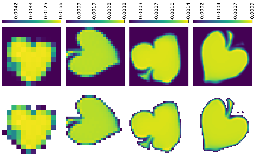
$12\times 12$          $25\times 25$          $40\times 40$          $50\times 50$

(a) Fixed-support barycenters computed using UMGW for different grid sizes. (Top) Computed measure on the full support. (Bottom) Computed measure restricted to the essential support.

RBCD ($\varepsilon_{1}$)      RBCD ($\varepsilon_{2}$)        BCD

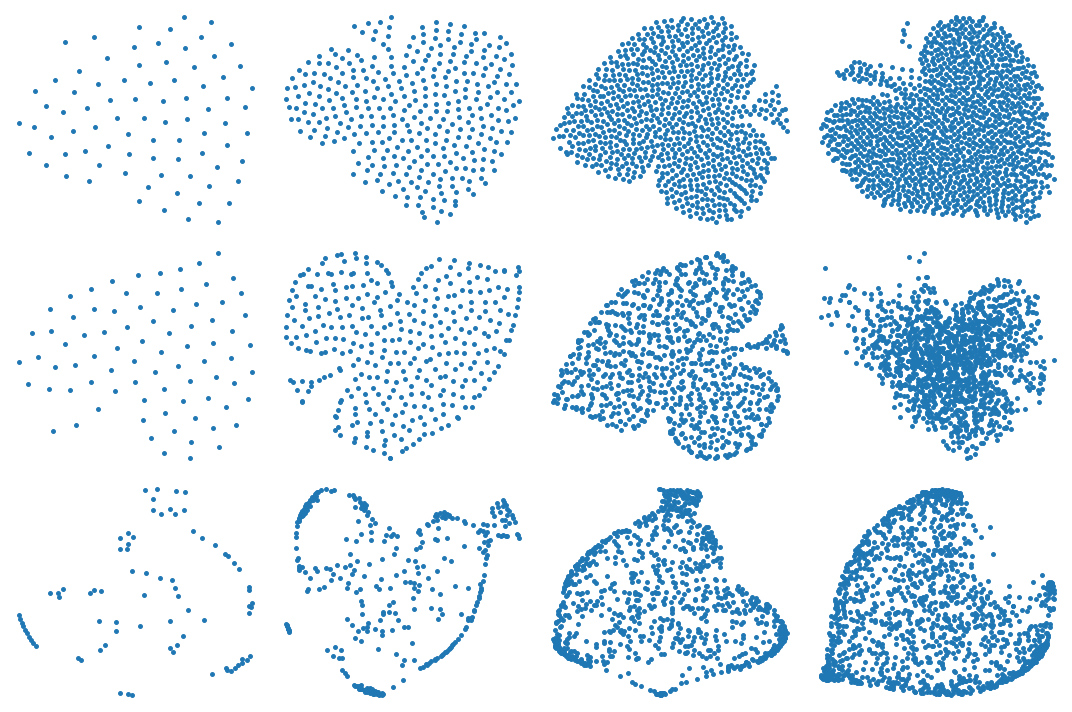
$81$              $348$              $901$              $1379$

(b) Free-support barycenters computed using (R)BCD for different numbers of support point. The regularization parameter is chosen as $\varepsilon_{1}\coloneqq 5\cdot 10^{-3}$ and $\varepsilon_{2}\coloneqq 5\cdot 10^{-4}$.

Figure 2: Comparison between the balanced barycenters between the images in Fig. 1 computed using UMGW (Remark 5.5) and (R)BCD (Remark 5.6). The UMGW barycenters are determined on full square grids of different sizes. The (R)BCD barycenters are computed using differed fixed numbers of support points and are embedded in 2d using MDS. The number of support points corresponds to the number of essential support points in the computed UMGW barycenters.

In this first example, we compare the UMGW method for fixed-support barycenters in Remark 5.5 with block coordinate descent (BCD) and its regularized version (RBCD) proposed by Peyré, Cuturi, and Solomon [41]. A brief summary of (R)BCD is given in Remark 5.6. As mentioned, our method requires us to fix the support beforehand and yields a measure on this support, whereas BCD and RBCD fix a discrete measure on a fixed number of support points and yield a dissimilarity matrix. For the latter procedures, we employ the implementations of the POT library [23]. For the numeric computations, we consider two $50\times 50$ pixel images of a spade and a heart, see Fig. 1, from which we extract the mm-spaces $\mathbb{X}_{1}$ and $\mathbb{X}_{2}$ with normalized Euclidean distances. Using the UMGW method in Remark 5.5 with $\varepsilon=0.15\cdot 10^{-3}$, $\rho_{1}\coloneqq\rho_{2}\coloneqq 0.5$, we compute several balanced barycenters on different grids in the image domain consisting of $12\times 12$, $25\times 25$, $40\times 40$, and $50\times 50$ pixels. The numerical computations are restricted to 200 seconds, and the resulting barycenters are shown in Fig. 2(a).

UMGW,   BCD,   RBCD ($\varepsilon_{2}$),   RBCD ($\varepsilon_{1}$)     
barycentric loss
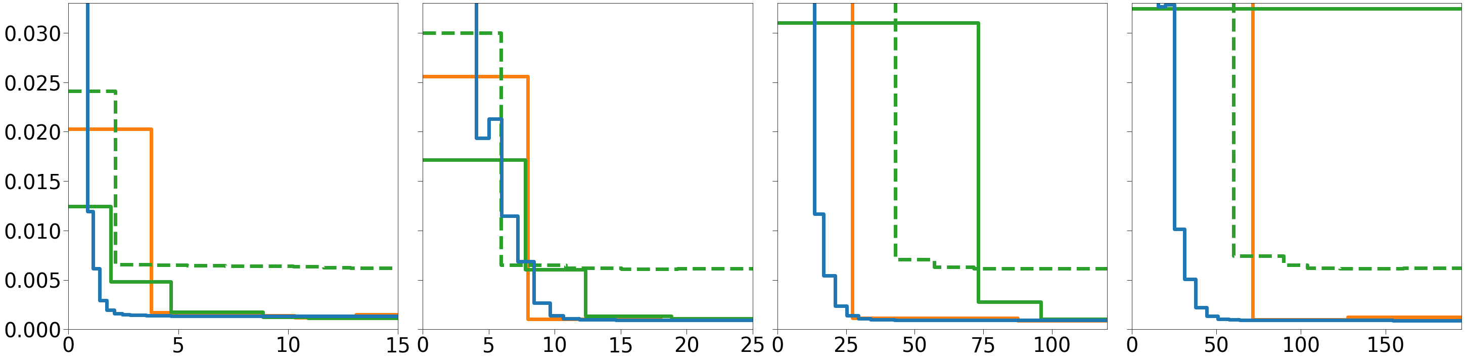
          $12\times 12$ grid,                 $25\times 25$ grid,                 $40\times 40$ grid,                 $50\times 50$ grid,
          $81$ points                      $348$ points                     $901$ points                    $1379$ points

Figure 3: Barycentric loss of the UMGW method and the (R)BCD method to compute the balanced barycenter between the images in Fig. 1 plotted against computation time in seconds. The loss is shows with respect to different grid sizes and numbers of support-points.

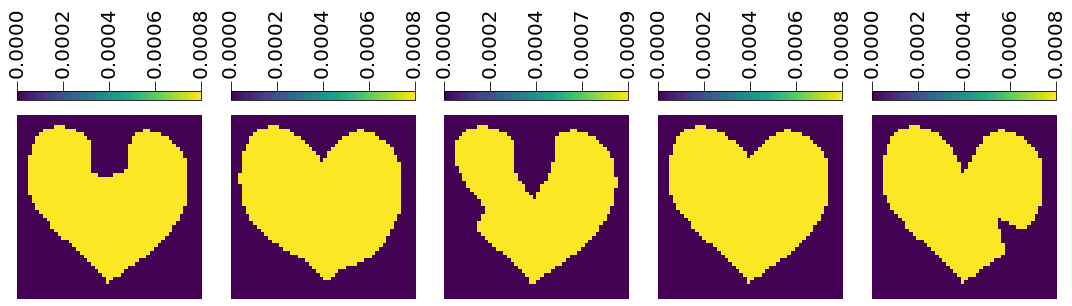
Figure 4: The ($50\times 50$)-pixel test images of the multi-input experiment in Section 7.1.

UMGW,   BCD,   RBCD ($\varepsilon_{2}$)       
barycentric loss
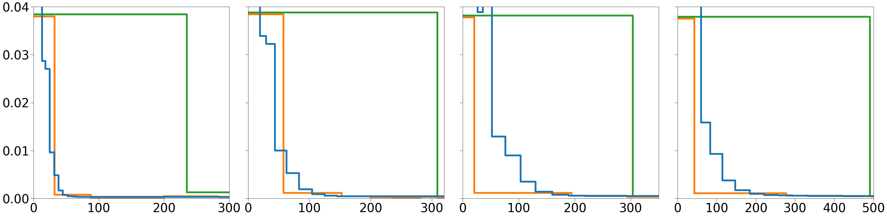
        2 inputs                   3 inputs                 4 inputs                   5 inputs

Figure 5: Barycentric loss of the UMGW method and the (R)BCD method to compute the balanced barycenter between several numbers of inputs from Fig. 1 plotted against computation time in seconds.

We proceed with with computing (R)BCD balanced barycenters, see Remark 5.6, where we initalize the (R)BCD method by a uniform distribution on a fixed number of support point. For a fair comparison, the number of support points is chosen with respect to the number of essential support points of the UMGW barycenters in Fig. 2(a), that is, to the number of pixels with mass greater than $10^{-4}$. Moreover, the computation time is again restricted to 200 seconds. For the regularized variant, we consider $\varepsilon_{1}\coloneqq 5\cdot 10^{-3}$ and $\varepsilon_{2}\coloneqq 5\cdot 10^{-4}$. Unfortunately, lower choices result in numerical errors. The outputs consist of dissimilarity matrices, which are embedded in two dimensions using multi-dimensional scaling (MDS). The embedded support-free barycenters are shown in Fig. 2(b).

Due to the rotational and reflectional invariance of GW, the computed barycenters in Fig. 2 do not follow any particular alignment. Moreover, the GW barycenter does not have to be unique. Despite the different nature of the barycenters (image or point cloud), the results for our UMGW-based method and BCD are qualitatively comparable. Considering the evolution of the barycentric loss $(\operatorname{GW}^{2}_{\varepsilon}(\mathbb{X}_{1},\mathbb{Y})+\operatorname{GW}^{2}_{\varepsilon}(\mathbb{X}_{2},\mathbb{Y}))/2$ over the computation time, our UMGW method perform similar well than (R)BCD, which substantiate the discussion in Remark 5.6 conjecturing that the complexity of both method is comparable. Increasing the number of inputs, see Fig. 4, which represent $50\times 50$ pixel images from the heart class in [12], we repeat the experiment to determine a balanced barycenter on a $50\times 50$ pixel grid using UMGW. For (R)BCD, the number of points is again chosen with respect to the number of essential pixels of the UMGW barycenter. Figure 5 shows the respective barycenter losses against time in seconds. Intriguingly, while BCD scales very well, and UMGW only slightly worse than BCD, the computation of RBCD increases dramatically.

7.2 Progressive Interpolation on Non-Euclidean Domains

In this example, we utilize the UMGW-based barycenter method in Remark 5.5 to calculate a progressive GW interpolation between measures on the unit sphere in $\mathbb{R}^{3}$. Using the standard spherical coordinates, we discretize the unit sphere by an $80\times 80$ pixel grid on $[0,2\pi]\times[0,\pi]$ and endow it with the normalized great circle distance. In this manner, we obtain a (discrete) metric space $(X,d_{X})$. Next, we equip $(X,d_{X})$ with measures representing the landmasses of the earth at two points in time. Here, $\mu_{1}$ corresponds to the distribution of Pangea, a supercontinent containing the entire landmass of the earth until the jurassic period. On the other hand, $\mu_{2}$ corresponds to the distribution of the today landmasses. These measures lead us to the mm-spaces $\mathbb{X}_{1}=(X,d_{X},\mu_{1})$ and $\mathbb{X}_{2}=(X,d_{X},\mu_{2})$. A visualization is given on the uttermost left-hand and right-hand side of Fig. 6. Note that the point masses around the poles become smaller to respect the denser discretization. Choosing $\varepsilon=3\cdot 10^{-3}$, we compute the balanced barycenters for $(\rho_{1},\rho_{2})=(0.8,0.2),(0.6,0.4),(0.4,0.6),(0.2,0.8)$. These barycenters are also shown in Fig. 6. Obtaining such an interpolation with BCD or RBCD is non-trivial as the mm-space corresponding to the resulting dissimilarity matrix needs to be embedded on the sphere, which poses an additional challenge. Clearly, the approach in this example can be applied to compute GW barycenters on arbitrary compact Riemannian manifolds.

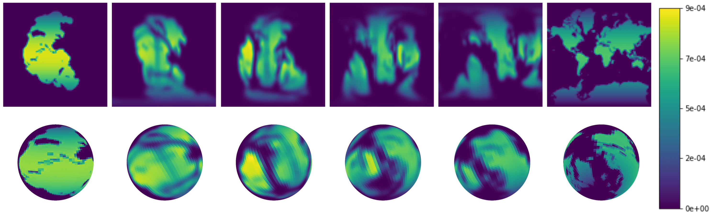
$\mathbb{X}_{1}$

$\mathbb{Y}_{1}$

$\mathbb{Y}_{2}$

$\mathbb{Y}_{3}$

$\mathbb{Y}_{4}$

$\mathbb{X}_{2}$

Figure 6: Progressive Gromov–Wasserstein interpolation via multi-marginal Gromov–Wasserstein transport in the balanced setting.

7.3 Fused Gromov–Wasserstein Barycenter of Labelled Images

In this section, we turn our attention to the computation of barycenters of shapes coming from 2D images which pixels admit a unique label. The following examples indicate that the fused version of our barycenter procedure yields desirable results when incorporating this additional label information.

For the first example, we consider the MNIST database [31], which consists of handwritten digits on a ($28\times 28$)-pixel grid. By concatenation and rotation of digits, we construct four ($30\times 34$)-pixel images containing the numbers 98 and 81, see the first two columns of Figs. 7 and 8. The images are again interpreted as mm-spaces. Furthermore, we label the different digits of the numbers. For this, we use the label space $(A,g)$ where $A\coloneqq\{0,1\}$ and $e$ is the Euclidean distance, and annotate the pixels of the first digit by $0$ and of the second digit by $1$. The (labelled) mm-spaces are shown in first two columns of Figs. 7 and 8. Here blue corresponds to label $0$ and red to label $1$.

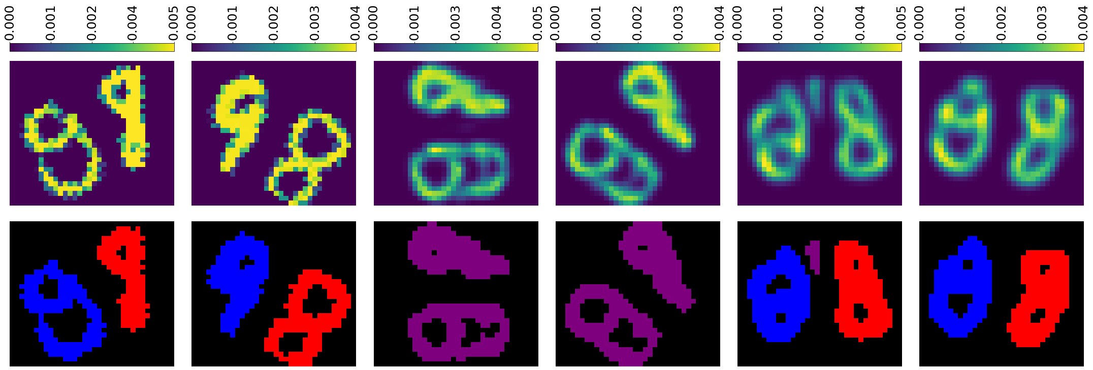
$\mathbb{X}_{1}$/$\mathfrak{X}_{1}$

$\mathbb{X}_{2}$/$\mathfrak{X}_{2}$

GW

UGW

FGW

FUGW

Figure 7: First row, left to right: input marginals, GW barycenter, UGW barycenter, FGW barycenter, UFGW barycenter. Second row, left to right: labels of the input marginals, visualized transport to the barycenters by averaging the label colour of the incoming mass.

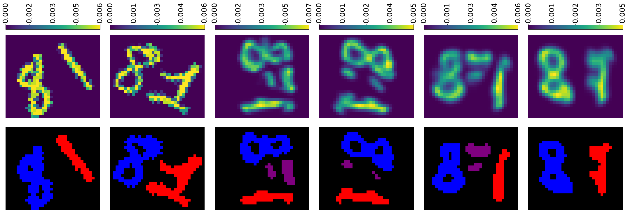
$\mathbb{X}_{1}$/$\mathfrak{X}_{1}$

$\mathbb{X}_{2}$/$\mathfrak{X}_{2}$

GW

UGW

FGW

FUGW

Figure 8: First row, left to right: input marginals, GW barycenter, UGW barycenter, FGW barycenter, UFGW barycenter. Second row, left to right: labels of the input marginals, visualized transport to the barycenters by averaging the label colour of the incoming mass.

To determine fixed-support barycenters, we apply Theorems 5.3 and 6.4, where the multi-marginal transport is computed by Algorithm 1. For this, we set the support and distance of the mm-space $\mathbb{Y}\coloneqq(Y,d_{Y},\bullet)$ according to a ($30\times 34$)-pixel image. Moreover, we choose $\mathfrak{Y}\coloneqq((Y_{1}\times\{1\})\cup(Y_{2}\times\{0\}),d,e,\bullet)$, where $Y_{1}$ and $Y_{2}$ corresponds to the left and right half of the pixel grid, respectively. We use the weights $\rho\coloneqq(0.5,0.5)$, a small regulatization by $\varepsilon\coloneqq 0.0002$, the divergence $\phi_{i}\coloneqq 0.01\,\phi_{\mathrm{BS}}$ for the unbalanced setting, and the trade-off parameter $\beta=0.5$ for the fused setting. We compute the GW, UGW, FGW, and UFGW barycenters presented in the first row of Figs. 7 and 8. As usual with $\operatorname{GW}$, the non-fused barycenters do not follow any particular alignment. However, In the fused case the correct alignment is enforced by our choice of labelling in Y. In the second row, the transport to the barycenter is visualized by averaging the label colours with respect to the transported (labelled) pixels to a certain point in the barycenter.

In Fig. 7, the shape of the eight in first space looks like the nine in the other space and vice versa. This is well reflected by the GW and UGW barycenters, which average the eight with the nine and the other way round. Due to the additional labels in the fused setup, the FGW and UFGW barycenter correspond to the matching of both nines and both eights. In the balanced case, some mass has to be transported between both digits resulting in an undesired artifact. Looking at the last barycenter, this can be avoided by using the unbalanced approach. In Fig. 8, both digits are matched in the correct order for all barycenters. Due to the mass variations between the digits, the GW, UGW, and FGW barycenter contain some artefacts between the digits. The unbalanced, fused approach can again avoid the unwanted artifacts.

Since the labels of the fused barycenters are here fixed in advanced, we automatically obtain an embedding of the barycenter such that the numbers are written upright. In both examples, the fused unbalanced Gromov–Wasserstein barycenter provides the best depiction of the numbers 98 and 81.

For the second example, we take two 2D shapes represented by ($64\times 64$)-pixel images from the previously mentioned publicly available database [12]. Both images are of the class “camel”. Similarly to above, we equip each pixel with a unique label. This time our label space $(A,e)$ is given by $A=\{0,1,2,3\}$ with distance

$$e(a,a^{\prime})\coloneqq\begin{cases}0&\text{if }a=a^{\prime}\\ 1&\text{if }|a-a^{\prime}\rvert=2\\ 1/2&\text{else.}\end{cases}$$

We associate the labels $0,1,2,3$ with the head, legs, tail, and hump, respectively. Notably, the metric $e$ admits the following interpretation: if two distinct body parts are direct neighbours, then their distance is $1/2$, otherwise the distance is $1$. The constructed spaces are shown in the first two columns of Fig. 9. We proceed as before and compute the barycenters with respect to the parameters $\rho\coloneqq(0.5,0.5)$, $\varepsilon=0.7\cdot 10^{-4}$, $\phi_{i}\coloneqq 0.01\,\phi_{\text{BS}}$, and $\beta=0.5$. For the non-fused case, we choose support and distance in $\mathbb{Y}\coloneqq(Y,d,\bullet)$ to be the same underlying ($64\times 64$)-pixel grid as the inputs. For the fused case, we consider the full Cartesian product $Y\times A$, i.e. $\mathfrak{Y}\coloneqq(Y\times A,d,e,\bullet)$. The computed GW, UGW, FGW, and UFGW barycenters are shown in Fig. 9.

Neither the balanced nor the unbalanced $\operatorname{GW}$ approach finds a meaningful barycenter, i.e. an image which illustrates a camel. Figuratively, these approaches match the head of one input with the hump of the other and vice versa. This incorrect matching results from large dissimilarity of the single features. The fused approaches, however, eliminate this issue by exploiting the label information and find a meaningful barycenter. The visualized transport also shows that in the balanced case two artifacts are present. Notably, the right artifact is orange and thus a result of transporting between the head in one input and the hump in the other. This implies large transport costs which explains why this particular artifact is not present in the unbalanced version while the other artifact is.

$\mathbb{X}_{1}$/$\mathfrak{X}_{1}$

$\mathbb{X}_{2}$/$\mathfrak{X}_{2}$

GW

UGW

FGW

FUGW

Figure 9: First row, left to right: input marginals, GW barycenter, UGW barycenter, FGW barycenter, UFGW barycenter. Second row, left to right: labels of the input marginals, visualized transport to the barycenters by averaging the label colour of the incoming mass.

$\mathbb{X}_{1}$                      $\mathbb{X}_{2}$                      $\mathbb{X}_{3}$                      $\mathbb{X}_{4}$                      $\mathbb{X}_{5}$
transferred image        clean image          noisy image
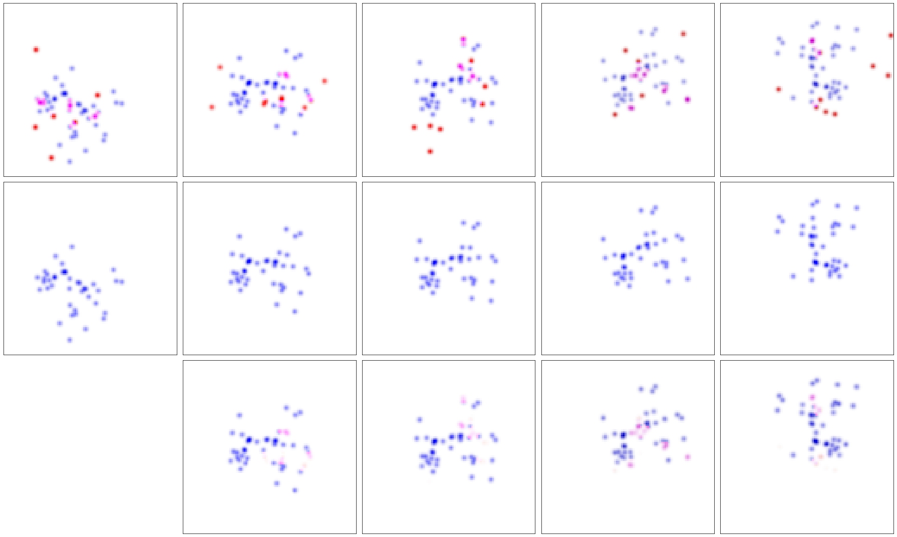
                            $\bm{K}_{1\to 2}\mu_{1}^{\mathrm{clean}}$         $\bm{K}_{1\to 3}\mu_{1}^{\mathrm{clean}}$         $\bm{K}_{1\to 4}\mu_{1}^{\mathrm{clean}}$         $\bm{K}_{1\to 5}\mu_{1}^{\mathrm{clean}}$

Figure 10: Synthetic snapshots for the numerical experiment in Section 7.4. The middle row contains the clean images of the dynamic of 40 coherent particles. The top row shows the noisy images, where every images contains 10 additional (noise) particles. The colour encodes clean particles (blau), noise particles (red), and the superposition of clean and noise particles (magenta). The bottom row shows the transferred first clean image by the computed transfer operators. The colour corresponds to the colour in the top row.

7.4 Estimating Transfer Operators of Particle Systems

In the final example, multi-marginal GW transport is used for the estimation of transfer operators. Mathematically, a transfer operator or Frobenius–Perron operator is linear map $K\colon L^{1}(\mathbb{X}_{1})\to L^{1}(\mathbb{X}_{2})$ describing the evolution of a dynamical system between two moments in time [24, 29]. Here $L^{1}(\mathbb{X}_{i})$ for $\mathbb{X}_{i}\coloneqq(X_{i},d_{i},\mu_{i})$ denotes the set of all absolutely integrable functions on $X_{i}$ with respect to $\mu_{i}$. The aim of this example is to recover the dynamical evolution of a coherent particle system from noisy observations. In this context, coherent means that the relative movement between coherent particles can be neglected. The synthetic data are generated as follows: Firstly, the positions of 40 coherent particles are sampled from the standard Gaussian on $\mathbb{R}^{2}$. Slowly rotating the coherent structure and moving it along some curve, we generate five snapshots of the particle system. To these snapshots, we add 10 further particles serving as noise. Equipping all particles with a uniform weight, applying a Gaussian filtering, and thresholding the resulting image values at $10^{-5}$, we obtain the synthetic observations in Fig. 10, where each snapshots consists of $100\times 100$ pixels and is interpreted as mm-space $\mathbb{X}_{i}$, $i=1,\dots,5$, like in the previous examples. The goal is to determine a transfer operator that describes the underlying movement by mapping the density of a single particle in one observation to the density of the corresponding particle in the next observation.

If the rotation of the system is insignificant, the transfer operator can be estimated using regularized, unbalanced Wasserstein transport [29, 5]. More precisely, having the matrix $\bm{\pi}$ corresponding to an optimal (regularized, unbalanced) transport plan between two observations—two measures on a joint, discrete metric space, we may estimate the transfer operator by the linear mapping $\bm{K}$ corresponding to the matrix

(24) $$\bm{K}^{\mathrm{T}}\coloneqq\operatorname{diag}(\bm{\pi}_{1})^{-1}\bm{\pi}\quad\text{with}\quad\bm{\pi}_{1}\coloneqq\bm{\pi}^{\mathrm{T}}\bm{1},$$

where $\bm{1}$ denotes the all-ones vector, and where $0^{-1}$ is set to $0$. The construction of $\bm{K}$ can be motivated using statistical physics [29], and the quality of $\bm{K}$ strongly depends on the quality of $\bm{\pi}$. Considering the five snapshots in Fig. 10, we notice that the particle system is significantly rotating anti-clockwise such that the Wasserstein transports $\bm{\pi}$ and the corresponding $\bm{K}$ do not match related particles between different observations.

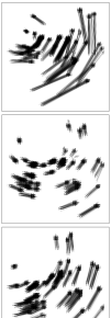
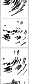
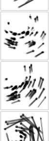
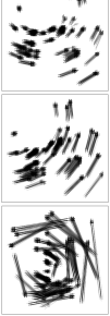
$\bm{K}_{1\to 2}$                          $\bm{K}_{2\to 3}$                          $\bm{K}_{3\to 4}$                          $\bm{K}_{4\to 5}$

Figure 11: The estimated transfer operators between the synthetic snapshots in Fig. 10. The arrows indicate to where the mass of a certain pixel is transferred. The gray values indicate the amount of mass which is transported. The figures contain only arrows corresponding to a mass transport larger than $10^{-4}$.

Differently from the Wasserstein distance, the Gromov–Wasserstein distance is invariant under rotations and translations, i.e. the GW plan between two snapshots $\mathbb{X}_{i}$ and $\mathbb{X}_{j}$ should match the related particles. On the basis of this observation, we propose to adapt the construction of the transfer operator $\bm{K}$ in Eq. 24 by replacing $\bm{\pi}$ with an optimal GW plan. To handle the noise particles and to estimate all transfer operators simultaneously, we compute an $\operatorname{UMGW}_{\varepsilon}$ plan $\bm{\pi}_{\operatorname{UMGW}}$ with $\varepsilon\coloneqq 0.2\cdot 10^{-3}$, where the marginals are unbalanced with respect to $10^{-3}\operatorname{KL}$. Having the evolution of the system over time in mind, we employ the cost function

$$c\coloneqq\sum_{i=1}^{4}|d_{i}-d_{i+1}|^{2}.$$

The transfer operator $\bm{K}_{i\to j}$ between the snapshots $\mathbb{X}_{i}$ and $\mathbb{X}_{j}$ is then estimated by

$$\bm{K}^{\mathrm{T}}_{i\to j}\coloneqq\operatorname{diag}(\bm{\pi}_{i})^{-1}(P_{X_{i}\times X_{j}})_{\#}\bm{\pi}_{\operatorname{UMGW}}\quad\text{with}\quad\bm{\pi}_{i}\coloneqq(P_{X_{i}})_{\#}\bm{\pi}_{\operatorname{UMGW}}.$$

The estimated operators $\bm{K}_{i\to i+1}$, $i=1,\dots,4$, are shown in Fig. 11. Despite the noise, the underlying dynamic (transition and rotation) between the snapshots is well recovered. Moreover, we use the estimated dynamic to propagate the first clean image $\mu_{1}^{\mathrm{clean}}$ to $\mathbb{X}_{i}$ by computing $\bm{K}_{1\to i}\mu_{1}^{\mathrm{clean}}$ for $i=2,\dots,5$. In this manner, we nearly recover the remaining clean images, see Fig. 10 bottom row. Notice that the computed transfer operators do not transfer mass from clean particles to well separated noise particles. This numerical example is just a first proof of concept that multi-marginal, unbalanced, regularized GW transports are able to recover dynamics where the Wasserstein transport would fail. This could be a starting point for further research about GW-based transfer operators.

8 Conclusions

We proposed the novel formulation of multi-marginal GW transport and its regularized, unbalanced and fused versions. By establishing the bi-convex relaxation and the barycenter relation, we provide new tools to compute fixed-support GW barycenters. We gave several examples showing that our procedure finds meaningful GW, UGW, FGW, and UFGW barycenters. Furthermore, we provided evidence that our procedure can also be used to create progressive GW interpolations or to denoise particle images. The employed bi-convex relaxation proved to be tight for appropriate cost functions in the balanced case. Up to now, we are not aware of a tightness argument in the unbalanced setting. The main problem is here that the marginals of $\pi$ and $\gamma$ do not have to coincide such that we cannot exploit the marginal conditionally negative definiteness. Also based on the bi-convex relaxation, we may ask what happens if the given marginals of the two underlying plans $\pi$ and $\gamma$ differ in general. This gives rise to a multi-marginal co-optimal transport formulation, whose discussion is left as future work.

Appendix A Proof of Proposition 3.1

The proof is based on properties of Csiszár divergences and the following properties of the product measure and integral operators.

Lemma A.1 (Product Measure, [9, Prop 2.7.8]).

Let $X$ be a Polish space. If $\pi_{n}\rightharpoonup\pi$ converges weakly in $\mathcal{M}^{+}(X)$, then $\pi_{n}\otimes\pi_{n}\rightharpoonup\pi\otimes\pi$ converges weakly in $\mathcal{M}^{+}(X\times X)$.

Lemma A.2 (Lower Semi-continuity).

Let $c\colon X\times X\to[0,\infty]$ be lower semi-continuous. Then the mapping $\pi\mapsto\int_{X\times X}c(x,x^{\prime})\,\mathrm{d}\pi(x)\,\mathrm{d}\pi(x^{\prime})$ is weakly lower semi-continuous.

Proof A.3.

For every lower semi-continuous $c$ bounded from below, there exists a sequence of (Lipschitz) continuous functions $(c_{k})_{k\in\mathbb{N}}$ with $c_{k}(x,x^{\prime})\uparrow c(x,x^{\prime})$ for all $x,x^{\prime}\in X$, cf. [56, p 67]. Let $\pi_{n}\rightharpoonup\pi$ be a weakly convergent sequence in $\mathcal{M}^{+}(X)$. Using Lemma A.1, we have

$$\liminf_{n\to\infty}\int_{X^{2}}c(x,x^{\prime})\,\mathrm{d}\pi_{n}(x)\,\mathrm{d}\pi_{n}(x^{\prime}) \geq\liminf_{n\to\infty}\int_{X^{2}}c_{k}(x,x^{\prime})\,\mathrm{d}\pi_{n}(x)\,\mathrm{d}\pi_{n}(x^{\prime})$$

$$=\int_{X^{2}}c_{k}(x,x^{\prime})\,\mathrm{d}\pi(x)\,\mathrm{d}\pi(x^{\prime})$$

for all $k\in\mathbb{N}$. Taking the supremum over $k\in\mathbb{N}$ and applying Lebesgue’s dominated convergence theorem establishes the weak lower semi-continuity.

Proof A.4 (Proof of Proposition 3.1).

The objective $F_{\varepsilon}$ in $\operatorname{UMGW}_{\epsilon}$ is weakly lower semi-continuous as sum of weakly lower semi-continuous functions. More precisely, the integral is weakly lower semi-continuous by Lemma A.2. The remaining terms of the sum are compositions of weakly lower semi-continuous divergences and the weakly continuous mappings $\pi\mapsto\pi\otimes\pi$, see Lemma A.1, and $\pi\mapsto(P_{X_{i}})_{\#}\pi=\pi_{i}$. By Jensen’s inequality, we know that for every $\mu,\nu\in\mathcal{M}^{+}(\mathcal{X})$ with $\|\nu\|_{\operatorname{TV}}>0$, it holds

$$D_{\phi}(\mu,\nu)\geq\|\nu\|_{\operatorname{TV}}\,\phi(\|\mu\|_{\operatorname{TV}}/\|\nu\|_{\operatorname{TV}}),$$

see [32, (2.44)]. Therefore, we may bound the objective from below by

$$\operatorname{F}_{\varepsilon}(\pi) \geq\sum_{i=1}^{N}D_{\phi_{i}}^{\otimes}(\pi_{i},\mu_{i})+\varepsilon\operatorname{KL}^{\otimes}(\pi,\nu^{\otimes})$$

$$\geq\sum_{i=1}^{N}\|\mu_{i}\|_{\operatorname{TV}}^{2}\,\phi_{i}\Bigl{(}\tfrac{\|\pi_{i}\|_{\operatorname{TV}}^{2}}{\|\mu_{i}\|_{\operatorname{TV}}^{2}}\Bigr{)}+\varepsilon\,\|\nu^{\otimes}\|_{\operatorname{TV}}^{2}\,\phi_{\operatorname{KL}}\Bigl{(}\tfrac{\|\pi\|_{\operatorname{TV}}^{2}}{\|\nu^{\otimes}\|_{\operatorname{TV}}^{2}}\Bigr{)}$$

$$=\|\pi\|_{\operatorname{TV}}^{2}\,\biggl{[}\sum_{i=1}^{N}\underbrace{\tfrac{\|\mu_{i}\|_{\operatorname{TV}}^{2}}{\|\pi\|_{\operatorname{TV}}^{2}}\,\phi_{i}\Bigl{(}\tfrac{\|\pi\|_{\operatorname{TV}}^{2}}{\|\mu_{i}\|_{\operatorname{TV}}^{2}}\Bigr{)}}_{\to(\phi_{i})^{\prime}_{\infty}}+\varepsilon\,\underbrace{\tfrac{\|\nu^{\otimes}\|_{\operatorname{TV}}^{2}}{\|\pi\|_{\operatorname{TV}}^{2}}\,\phi_{\operatorname{KL}}\Bigl{(}\tfrac{\|\pi\|_{\operatorname{TV}}^{2}}{\|\nu^{\otimes}\|_{\operatorname{TV}}^{2}}\Bigr{)}}_{\to\infty}\biggr{]}.$$

For both assumptions, $F_{\varepsilon}(\pi)$ diverges for $\|\pi\|\to\infty$ showing coercivity. Consequently, every minimizing sequence $(\pi^{(n)})_{n\in\mathbb{N}}\in\mathcal{M}^{+}(X)$ with $F_{\varepsilon}(\pi^{(n)})\downarrow\operatorname{UMGW}_{\varepsilon}(\mathbb{X}_{1},\dots,\mathbb{X}_{N})$ is uniformly bounded in total variation. The theorem of Banach–Alaoglu guarantees the existence of a weakly convergent subsequence $\pi^{(k)}\rightharpoonup\tilde{\pi}\in\mathcal{M}^{+}(X)$. The weak lower semi-continuity of $F_{\varepsilon}$ ensures that $\tilde{\pi}$ is a minimizer.

References

- [1] J. M. Altschuler and E. Boix-Adsera. Polynomial-time algorithms for multimarginal optimal transport problems with decomposable structure. arXiv:2008.03006, 2020.
- [2] L. Ambrosio, E. Brué, and D. Semola. Lectures on Optimal Transport. Number 130 in Unitext. Springer, Cham, 2021.
- [3] E. Anderes, S. Borgwardt, and J. Miller. Discrete Wasserstein barycenters: optimal transport for discrete data. Math. Methods Oper. Res., 84(2):389–409, 2016.
- [4] F. Beier, R. Beinert, and G. Steidl. On a linear Gromov-Wasserstein distance. arXiv:2112.11964, 2021.
- [5] F. Beier, J. von Lindheim, S. Neumayer, and G. Steidl. Unbalanced multi-marginal optimal transport. arXiv:2103.10854, 2021.
- [6] R. Beinert, C. Heiss, and G. Steidl. On assignment problems related to Gromov–Wasserstein distances on the real line. arXiv:2205.09006, 2022.
- [7] J.-D. Benamou, G. Carlier, and L. Nenna. A numerical method to solve multi-marginal optimal transport problems with Coulomb cost. In Splitting Methods in Communication, Imaging, Science, and Engineering, pages 577–601. Springer, Cham, 2016.
- [8] J.-D. Benamou, G. Carlier, and L. Nenna. Generalized incompressible flows, multi-marginal transport and Sinkhorn algorithm. Numer. Math., 142(1):33–54, 2019.
- [9] V. I. Bogachev. Weak convergence of measures, volume 234 of Mathematical Surveys and Monographs. American Mathematical Society, Providence, RI, 2018.
- [10] E. Bogomolny, O. Bohigas, and C. Schmit. Distance matrices and isometric embedding. J. Math. Phys. Anal. Geom., 4(1):7–23, 2008.
- [11] L. Brogat-Motte, R. Flamary, C. Brouard, J. Rousu, and F. d’Alché Buc. Learning to predict graphs with fused Gromov–Wasserstein barycenters. arXiv:2202.03813, 2022.
- [12] A. Carlier, K. Leonard, S. Hahmann, G. Morin, and M. Collins. The 2D shape structure dataset. https://2dshapesstructure.github.io.
- [13] G. Carlier and I. Ekeland. Matching for teams. Econ. Theory, 42(2):397–418, 2010.
- [14] Y. Chen and J. Karlsson. State tracking of linear ensembles via optimal mass transport. IEEE Contr. Syst. Lett., 2(2):260–265, 2018.
- [15] L. Chizat, G. Peyré, B. Schmitzer, and F.-X. Vialard. Scaling algorithms for unbalanced optimal transport problems. Math. Comp., 87(314):2563–2609, 2018.
- [16] L. Chizat, G. Peyré, B. Schmitzer, and F.-X. Vialard. Unbalanced optimal transport: Dynamic and Kantorovich formulations. J. Funct. Anal., 274(11):3090–3123, 2018.
- [17] S. Cohen, K. S. S. Kumar, and M. P. Deisenroth. Sliced multi-marginal optimal transport. arXiv:2102.07115, 2021.
- [18] M. Colombo, L. De Pascale, and S. Di Marino. Multimarginal optimal transport maps for one-dimensional repulsive costs. Canad. J. Math., 67(2):350–368, 2015.
- [19] M. Cuturi. Sinkhorn distances: Lightspeed computation of optimal transport. In Advances in Neural Information Processing Systems 26, pages 2292–2300. Curran Associates, Inc., 2013.
- [20] M. Cuturi and A. Doucet. Fast computation of Wasserstein barycenters. In Proc. Mach. Learn. Res., volume 32, pages 685–693. PMLR, 2014.
- [21] F. Elvander, I. Haasler, A. Jakobsson, and J. Karlsson. Multi-marginal optimal transport using partial information with applications in robust localization and sensor fusion. Signal Process., 171:107474, 2020.
- [22] A. Feragen, F. Lauze, and S. Hauberg. Geodesic exponential kernels: When curvature and linearity conflict. In 2015 IEEE Conference on Computer Vision and Pattern Recognition (CVPR), pages 3032–3042, 2015.
- [23] R. Flamary, N. Courty, A. Gramfort, M. Z. Alaya, A. Boisbunon, S. Chambon, L. Chapel, A. Corenflos, K. Fatras, N. Fournier, L. Gautheron, N. T. Gayraud, H. Janati, A. Rakotomamonjy, I. Redko, A. Rolet, A. Schutz, V. Seguy, D. J. Sutherland, R. Tavenard, A. Tong, and T. Vayer. POT: Python optimal transport. J. Mach. Learn. Res., 22(78):1–8, 2021.
- [24] G. Froyland. An analytic framework for identifying finite-time coherent sets in time-dependent dynamical systems. Phys. D, 250:1–19, 2013.
- [25] W. Gangbo and A. Świȩch. Optimal maps for the multidimensional Monge–Kantorovich problem. Comm. Pure Appl. Math., 51(1):23–45, 1998.
- [26] A. Gerolin, A. Kausamo, and T. Rajala. Multi-marginal entropy-transport with repulsive cost. Calc. Var. Partial Differ. Equ., 59(3):90, 2020.
- [27] I. Haasler, A. Ringh, Y. Chen, and J. Karlsson. Multimarginal optimal transport with a tree-structured cost and the Schrödinger bridge problem. SIAM J. Control Optim., 59(4):2428–2453, 2021.
- [28] T. Kerdoncuff, R. Emonet, M. Perrot, and M. Sebban. Optimal tensor transport. In Proceedings of the AAAI Conference on Artificial Intelligence, volume 36, pages 7124–7132, 2022.
- [29] P. Koltai, J. von Lindheim, S. Neumayer, and G. Steidl. Transfer operators from optimal transport plans for coherent set detection. arXiv:2006.16085, 2020.
- [30] K. Le, D. Le, H. Nguyen, D. Do, T. Pham, and N. Ho. Entropic Gromov-Wasserstein between Gaussian distributions. arXiv:2108.10961, 2021.
- [31] Y. Lecun, L. Bottou, Y. Bengio, and P. Haffner. Gradient-based learning applied to document recognition. Proc. IEEE, 86(11):2278–2324, 1998.
- [32] M. Liero, A. Mielke, and G. Savaré. Optimal entropy-transport problems and a new Hellinger–Kantorovich distance between positive measures. Invent. Math., 211(3):969–1117, 2018.
- [33] T. Lin, N. Ho, X. Chen, M. Cuturi, and M. Jordan. Fixed-support Wasserstein barycenters: Computational hardness and fast algorithm. In H. Larochelle, M. Ranzato, R. Hadsell, M. F. Balcan, and H. Lin, editors, Advances in Neural Information Processing Systems, volume 33, pages 5368–5380. Curran Associates, Inc., 2020.
- [34] H. Maron and Y. Lipman. (Probably) concave graph matching. In S. Bengio, H. Wallach, H. Larochelle, K. Grauman, N. Cesa-Bianchi, and R. Garnett, editors, Advances in Neural Information Processing Systems, volume 31. Curran Associates, Inc., 2018.
- [35] F. Mémoli. Gromov–Wasserstein distances and the metric approach to object matching. Found. Comput. Math., 11(4):417–487, 2011.
- [36] S. Neumayer and G. Steidl. From optimal transport to discrepancy. Handbook of Mathematical Models and Algorithms in Computer Vision and Imaging, 2020.
- [37] D. H. Nguyen and K. Tsuda. On a linear fused Gromov–Wasserstein distance for graph structured data. arXiv:2203.04711, 2022.
- [38] K. Nguyen, S. Nguyen, N. Ho, T. Pham, and H. Bui. Improving relational regularized autoencoders with spherical sliced fused Gromov Wasserstein. In International Conference on Learning Representations, 2021. https://openreview.net/forum?id=DiQD7FWL233.
- [39] B. Pass. Multi-marginal optimal transport: Theory and applications. ESAIM Math. Model. Numer. Anal., 49(6):1771–1790, 2015.
- [40] G. Peyré and M. Cuturi. Computational optimal transport: With applications to data science. Found. Trends Mach. Learn., 11(5-6):355–607, 2019.
- [41] G. Peyré, M. Cuturi, and J. Solomon. Gromov-Wasserstein averaging of kernel and distance matrices. In International Conference on Machine Learning, pages 2664–2672, 2016.
- [42] G. Peyré, M. Cuturi, and J. Solomon. Gromov-Wasserstein learning for graph matching and node embedding. In International Conference on Machine Learning, pages 6932–6941, 2019.
- [43] J. Rabin, G. Peyré, J. Delon, and M. Bernot. Wasserstein barycenter and its application to texture mixing. In International Conference on Scale Space and Variational Methods in Computer Vision, pages 435–446. Springer, 2011.
- [44] A. Salmona, J. Delon, and A. Desolneux. Gromov-Wasserstein distances between Gaussian distributions. arXiv:2104.07970, 2021.
- [45] F. Santambrogio. Optimal Transport for Applied Mathematicians, volume 87 of Progress in Nonlinear Differential Equations and their Applications. Birkhäuser/Springer, Cham, 2015. Calculus of variations, PDEs, and modeling.
- [46] I. J. Schoenberg. Metric spaces and completely monotone functions. Ann. Math., 39(4):811–841, 1938.
- [47] T. Sejourne, F.-X. Vialard, and G. Peyré. The unbalanced Gromov Wasserstein distance: Conic formulation and relaxation. In Advances in Neural Information Processing Systems, volume 34. Curran Associates, Inc., 2021.
- [48] S. Srivastava, C. Li, and D. B. Dunson. Scalable Bayes via barycenter in Wasserstein space. J. Mach. Learn. Res., 19:Paper No. 8, 35, 2018.
- [49] K.-T. Sturm. The space of spaces: curvature bounds and gradient flows on the space of metric measure spaces. arXiv:1208.0434, 2020.
- [50] T. Séjourné, J. Feydy, F.-X. Vialard, A. Trouvé, and G. Peyré. Sinkhorn divergences for unbalanced optimal transport. arXiv:1910.12958, 2019.
- [51] A. Thual, H. Tran, T. Zemskova, N. Courty, R. Flamary, S. Dehaene, and B. Thirion. Aligning individual brains with fused unbalanced Gromov Wasserstein. In S. Koyejo, S. Mohamed, A. Agarwal, D. Belgrave, K. Cho, and A. Oh, editors, Advances in Neural Information Processing Systems, volume 35, pages 21792–21804. Curran Associates, Inc., 2022.
- [52] V. Titouan, R. Flamary, N. Courty, R. Tavenard, and L. Chapel. Sliced Gromov-Wasserstein. In H. Wallach, H. Larochelle, A. Beygelzimer, F. Alché-Buc, E. Fox, and R. Garnett, editors, Advances in Neural Information Processing Systems, volume 32. Curran Associates, Inc., 2019.
- [53] V. Titouan, I. Redko, R. Flamary, and N. Courty. Co-optimal transport. Advances in Neural Information Processing Systems, 33:17559–17570, 2020.
- [54] Q. H. Tran, H. Janati, N. Courty, R. Flamary, I. Redko, P. Demetci, and R. Singh. Unbalanced co-optimal transport. arXiv:2205.14923, 2022.
- [55] T. Vayer, L. Chapel, R. Flamary, R. Tavenard, and N. Courty. Fused Gromov–Wasserstein distance for structured objects. Algorithms, 13(9):212, 2020.
- [56] C. Villani. Optimal Transport: Old and New, volume 338. Springer, 2008.
- [57] J. von Lindheim. Simple approximative algorithms for free-support barycenters. arXiv:2203.05267, 2022.
- [58] H. Wendland. Scattered Data Approximation, volume 17 of Cambridge Monographs on Applied and Computational Mathematics. Cambridge University Press, Cambridge, 2004.
- [59] H. Xu, D. Luo, and L. Carin. Scalable Gromov-Wasserstein learning for graph partitioning and matching. In H. Wallach, H. Larochelle, A. Beygelzimer, F. d'Alché-Buc, E. Fox, and R. Garnett, editors, Advances in Neural Information Processing Systems, volume 32. Curran Associates, Inc., 2019.