Spatial entanglement in two dimensional QCD:
Renyi and Ryu-Takayanagi entropies

Abstract

We derive a general formula for the replica partition function in the vacuum state, for a large class of interacting theories with fermions, with or without gauge fields, using the equal-time formulation on the light front. The result is used to analyze the spatial entanglement of interacting Dirac fermions in two-dimensional QCD. A particular attention is paid to the issues of infrared cut-off dependence and gauge invariance. The Renyi entropy for a single interval, is given by the rainbow dressed quark propagator to order ${\cal O}(N_{c})$. The contributions to order ${\cal O}(1)$, are shown to follow from the off-diagonal and off mass-shell mesonic T-matrix, with no contribution to the central charge. The construction is then extended to mesonic states on the light front, and shown to probe the moments of the partonic PDFs for large LF separations. In the vacuum and for small and large intervals, the spatial entanglement entropy following from the Renyi entropy, is shown to be in agreement with the Ryu-Takayanagi geometrical entropy, using a soft-wall AdS₃ model of two-dimensional QCD.

I Introduction

Quantum entanglement is paramount in quantum mechanics. It follows from the fact that quantum states are mostly superposition states, and two acausally related measurements can be correlated. A quantitative measure of this correlation is given by the entanglement entropy, with a number of applications in quantum many body systems and also quantum field theory Srednicki (1993); Calabrese and Cardy (2004); Casini et al. (2005); Hastings (2007); Calabrese and Cardy (2009).

The increase interest in entanglement, especially in lower dimensional systems, is partly motivated by recent developments in quantum information theory. Of particular interest, is the concept of entanglement entropy as a measure of quantum information flow Bremermann (1967); Bekenstein (1981). There is a large effort currently underway for a better theoretical and experimental understanding of entanglement in the nuclear many body problem Kaufman et al. (2016), the prompt thermalization at RHIC Stoffers and Zahed (2013); Qian and Zahed (2015a); Berges et al. (2019); Florio and Kharzeev (2021); Liu et al. (2022a), hadron tomography through DIS Kharzeev and Levin (2017); Liu et al. (2022b, a), and parton-parton scattering at low-x Stoffers and Zahed (2013); Qian and Zahed (2015b); Kharzeev and Levin (2017); Shuryak and Zahed (2018); Liu and Zahed (2019); Armesto et al. (2019); Dvali and Venugopalan (2021).

Recently, we have shown how entanglement in longitudinal parton-x, and also in rapidity space or ${\rm ln}\frac{1}{x}$, can be used to gain more insights on the partonic PDFs (large-x) and structure functions (small-x), using two-dimensional QCD. Recall tha 2D QCD is solvable in the large number of colors limit ’t Hooft (1974); Bars (1976). This allows for a quantitative understanding of the role played by the entanglement entropy, for single meson states, or their stringy form by resummation along a Regge trajectory. Remarkably, the entanglement entropy carried by a 2D nucleus on the light front, shows a growth rate with rapidity at the current bound on quantum information flow.

Spatial entanglement in interacting theories, and especially gauge theories is challenging. The geometrical construction proposed by Ryu-Takayanagi Ryu and Takayanagi (2006) in the context of a holographic dual gauge theories at large $N_{c}$ and strong gauge coupling, in this sense is rather remarkable. In interacting gauge theories with fermions, the dual descriptions are only approximate, and using them to analyze the entanglement geometrically is interesting, especially if large $N_{c}$ arguments can be used for a comparison.

Entanglement in two-dimensional QCD is intricate, as it involves interacting fermions with a dynamical gauge field. To address it, we use the replica construction in real time, by duplicating Minkowski space-time $n$ times, and then gluing the duplicates together, using pertinent twists of the replicated fermion fields. This procedure makes the ensuing Renyi entropy and its limiting entanglement entropy, gauge dependent in any dimension. This notwithstanding, both entropies can be evaluated by gauge fixing both in the continuum or on the lattice. For two-dimensional QCD, we will show that in the regular cut-off gauge, the large $N_{c}$ results are found to be in agreement with a soft-wall holographic construction, for very small or very large intervals. For completeness, we note that a replica analysis of two-dimensional QCD was suggested in Goykhman (2015), using different arguments.

The paper is organized as follows: In section II, we briefly review the replica construction of the Renyi entropy, and its relation to the entanglement entropy. We will also recall the form of the monodromy matrix that allows for the gluing of the fermionic replicas. In particular, we will derive a new equal-time representation of the replica partition function. In section III, we discuss the subtleties related to the gauge symmetry following from the gluing of the fermions, and why gauge fixing is required across the gluing cut. We will analyse the replica partition function, both in perturbation theory and in the large $N_{c}$ limit of 2D QCD, in the light front gauge. In section IV, we extend our replica construction to the spatial entanglement in partonic as well as hadronic states on the light front. For the latter, the entanglement is controlled by the moments of the partonic PDFs in 2D QCD. We suggest that these moments can be extracted from the Renyi entropy for space-like intervals in a fast moving hadron in 4D QCD, using current lattice QCD simulations. In section V, The leading results of the entanglement entropy both for small and large intervals, are shown to be compatible with the Ryu-Takayanagi entropy, using a soft-wall gravity dual to 2D QCD. Our conclusions are in section VI.

II Replica partition function and Renyi entropy

Let $\rho$ be the density of a pure state defined in a Hilbert space composed of two complementary regions $I$ and its complementary $\bar{I}$. For simplicity, we first focus on spatial regions. The projected or reduced density matrix in $\bar{I}$ obtained by tracing over $I$, is Calabrese and Cardy (2009); Casini et al. (2005)

$$\rho_{I}={\rm Tr}_{\bar{I}}\rho$$ (1)

Although $\rho$ carries zero von Neumann entropy, $\rho_{I}$ does not,

$$S=-{\rm Tr}_{I}(\rho_{I}\,{\rm log}\,\rho_{I})$$ (2)

which is a measure of the quantum entanglement between $I$ and $\bar{I}$ in $\rho$. To evaluate (2) one uses the Replica trick through the Renyi entropy $S_{n}$

$$S_{n}=\frac{1}{1-n}\ln{\rm tr}\rho_{\rm I}^{n}\equiv\frac{1}{1-n}\ln Z_{n}\ .$$ (3)

If $Z_{n}$ is analytic in $n$ in a neighborhood of $n=1$ with the Taylor-expanded form:

$$\ln Z_{n}=(n-1)Z^{(1)}+(n-1)^{2}Z^{(2)}+...\ ,$$ (4)

then the Shannon entropy or the entanglement entropy can simply be identified as

$$S={\lim_{n\to 1}}S_{n}=-Z^{(1)}=-{\lim_{n\to 1}}\frac{\partial}{\partial n}\ln Z_{n}\ .$$ (5)

We now show how to derive the replica partition function using the equal time formulation, valid for any interacting fermionic theory, in any dimension.

II.1 Fermionic monodromy

Using the transfer matrix, Calabrese and Cardy Calabrese and Cardy (2004, 2009) have shown that $Z_{n}$ for integer value of $n$, can be rewritten as an Euclidean path integral with fields living in a replica space. More specifically, a path integral with $n$ identical copies of the original Euclidean space, glued together along the single spatial cut corresponding to the region $I$, with twisted fermionic boundary conditions.

For a fermionic theory one has for $i=1,...n$ replicated fermions $\psi_{i}$, each living in its own manifold, this patching corresponds to twisting the fermions in going from one patch to the other Calabrese and Cardy (2009); Casini et al. (2005)

$$\bigg{[}{\cal T}_{n}\bigg{]}\begin{pmatrix}\psi_{1}\\ \psi_{2}\\ \vdots\\ \psi_{n}\end{pmatrix}=\begin{pmatrix}0&1&0&\cdots&0\\ 0&0&1&\cdots&0\\ \vdots&\vdots&\ddots&\vdots&1\\ (-1)^{n+1}&0&0&\cdots&0\end{pmatrix}\begin{pmatrix}\psi_{1}\\ \psi_{2}\\ \vdots\\ \psi_{n}\end{pmatrix}$$ (6)

The eigenvalues of the monodromy ${\cal T}_{n}$ are the n-roots of unity $e^{i2\pi k/n}$ with $k=-\frac{n-1}{2},...,+\frac{n-1}{2}$. This amounts to n-multi-valued fermions in a single-cut space $I=[a_{1},a_{2}]$, with each species $\psi_{k}$ picking a phase $e^{i2\pi k/n}$ phase in circling the left-edge ($a_{1}$) of the cut clock-wise, and $e^{-i2\pi k/n}$ in circling the right-edge ($a_{2}$) of the cut counter-clock-wise.

II.2 Equal-time representation of $Z_{n}$

In a Hamiltonian formulation of the replica in Minkowski signature, the gluing conditions are the new and key elements to add to the original field theory. We first consider the case of only fermionic theories with a single spatial cut, and the gluing conditions for the fermions given in (6). To construct the replica partition function for the vaccum of interacting fermions, we start from the generic off-diagonal matrix element of the vacuum density matrix $|\Omega\rangle\langle\Omega|$

$$\langle\psi_{0^{-}}|\Omega\rangle\langle\Omega|-\psi_{0^{+}}\rangle=\langle\Omega|\psi_{0^{+}}\rangle\langle\psi_{0^{-}}|\Omega\rangle\ ,$$ (7)

where $|\psi_{0^{\pm}}\rangle$ refer to two generic fermionic coherent states (their precise relation to the single space-time cut and labeling, will be detailed below). Here $|\Omega\rangle$ refers to the lowest energy state, prepared using the long time evolution, with the full fermionic Hamiltonian $H(\psi^{\dagger},\psi)$

$$|\Omega\rangle=e^{-iH[\psi^{\dagger},\psi]\frac{T}{2}(1-i0)}|\psi_{-\infty}\rangle\ .$$ (8)

starting from an arbitrary asymptotic coherent state $|\psi_{-\infty}\rangle$, whose explicit form is not needed. The additional minus sign in (7) is due to the Grassmannian nature of the states, when moving $\langle\psi_{0^{-}}|\Omega\rangle$ from left to right. Also, it is important that the density matrix $|\Omega\rangle\langle\Omega|$ is bosonic, namely, when expanded as polynomials in the Grassmannians, the order of each term must be even.

With this in mind, and to proceed to a path integral, we use the decomposition

$$e^{-iHT/2}=e^{-iH\epsilon}e^{-iH\epsilon}e^{-iH\epsilon}...e^{-iH\epsilon}$$

and insert the completeness relation between any of the two evolution operators

$${\bf 1}=\int d\bar{\psi}_{t}d\psi_{t}e^{-\bar{\psi}_{t}\psi_{t}}|\psi_{t}\rangle\langle\psi_{t}|\ ,$$ (9)

As a result, the matrix element in (7) can be cast in a standard path-integral form

$$\langle\Omega|\psi_{0^{+}}\rangle\langle\psi_{0^{-}}|\Omega\rangle=\int\prod_{t}d\bar{\psi}_{t}d\psi_{t}e^{\sum-\bar{\psi}_{t}(\psi_{t}-\psi_{t-1})-i\epsilon H[\bar{\psi}_{t},\psi_{t-1}]}\ ,$$ (10)

with no $-\bar{\psi}_{0^{+}}\psi_{0^{-}}$ term in the exponent. (10) is a path-integral representation of the density matrix in real time, for a single fermion species. To represent the trace, we need the completeness relation and the trace formula

$${\rm Tr}A=\int d\bar{\psi}d\psi e^{-\bar{\psi}\psi}\langle-\psi|A|\psi\rangle\ ,$$ (11)

in terms of which, we have

$${\rm Tr\rho_{I}^{n}}=\int\prod_{k=0}^{n-2}d\bar{\psi}_{k,0^{-}}d\psi_{k,0^{-}}e^{-\sum_{k=0}^{n-1}\sum_{x}\bar{\psi}_{k,0^{-}}(x)\psi_{k,0^{-}}(x)}$$

$$\prod_{k=0}^{n-1}\langle\Omega|-\psi_{k-1,0^{-}}(x\in I),\psi_{k,0^{-}}(x\notin I)\rangle\langle\psi_{k,0^{-}}(x\in I),\psi_{k,0^{-}}(x\notin I)|\Omega\rangle\ ,$$ (12)

where in the last equation one has made explicit the dependence on $x$ and $\psi_{0-1,0^{-}}=-\psi_{n-1,0^{-}}$. The above can then be represented as a path-integral in the replica space time with $n$ replica fermions species and with the gluing boundary condition across the boundary $I$ as indicated explicitly as in the equation above.

More specifically, the $n$’th trace can be written as a path integral with $i=0,1,..n-1$ copies of the fermion fields $\psi_{i,t}(x)$. Here $i$ refers to the replica index, $t$ to the time slice and $x$ to the spatial coordination of the Grassmannian. The twisting across the cut amounts to $\psi_{i,0^{+}}(x\in I)=-\psi_{i-1,0^{-}}(x\in I)$ for $i=1,2,...n-1$ and $\psi_{-1,0^{+}}(x\in I)=-\psi_{n-1,0^{-}}(x\in I)$, as illustrated in Fig. 1. Outside the cut, we have $\psi_{i,0^{+}}(x\notin I)=\psi_{i,0^{-}}(x\notin I)$. Now, using the charge conservation of the Hamiltonian, one can flip all the Grassmannians for old $i=2k-1$

$$\langle\Omega|-\psi_{2k-2,0^{-}}(x\in I),\psi_{2k-1}(x\notin I)\rangle\langle\psi_{2k-1,0^{-}}(x\in I),\psi_{2k-1,0^{-}}(x\notin I)|\Omega\rangle$$

$$\equiv \langle\Omega|\psi_{2k-2,0^{-}}(x\in I),-\psi_{2k-1}(x\notin I)\rangle\langle-\psi_{2k-1,0^{-}}(x\in I),-\psi_{2k-1,0^{-}}(x\notin I)|\Omega\rangle\ ,$$ (13)

and redefine for old $i$ (including $n-1$ if $n$ is even)

$$\psi_{2k-1,0^{-}}(x)\rightarrow-\psi_{2k-1,0^{-}}(x)\ .$$ (14)

Clearly, after these transformations, one has the alternative boundary condition $\psi_{i+1,0^{+}}(x\in I)=\psi_{i,0^{-}}(x\in I)$ for $i=0,1,2,...n-2$ and $\psi_{1,0^{+}}(x\in I)=(-1)^{n+1}\psi_{n-1,0^{-}}(x\in I)$, and for $x\notin I$ one needs no sign change. In terms of the independent variables $\psi_{i,0^{-}}(x)$, one has in the exponential for fermions along the cut or $x\in I$

$$\sum_{i}\bar{\psi}_{i,1}(x\in I)\psi_{i-1,0^{-}}(x\in I)-\sum_{i}\bar{\psi}_{i,0^{-}}(x\in I)\bigg{(}\psi_{i,0^{-}}(x\in I)-\psi_{i,-1}(x\in I)\bigg{)}$$ (15)

where $\psi_{-1,0^{-}}(x\in I)=(-1)^{n+1}\psi_{n-1,0^{-}}(x\in I)$ according to the boundary condition, in addition to the Hamiltonian term

$$-i\epsilon\sum_{i,x}H\bigg{[}\bar{\psi}_{i,1}(x),\psi_{i-1,0^{-}}(x\in I),\psi_{i,0^{-}}(x\notin I)\bigg{]}-i\epsilon\sum_{i}H\bigg{[}\bar{\psi}_{i,0^{-}}(x),\psi_{i,-1}(x)\bigg{]}\ .$$ (16)

This finishes the derivation of the replica partition function in real time, with the twisted boundary conditions across the cut $I$, as illustrated in Fig. 1 for $n=3$. Each strip in Minkowski space-time is cut at the initial times $t=0^{\pm}$, which is shown in dashed lines, with the fermionic field assignments $\psi_{i,0^{\pm}}(x\in I)$.

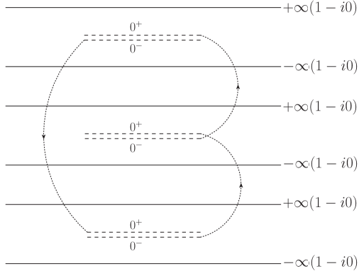
Figure 1: Replica Minkowski space-time for $n=3$. The boundaries for the time evolution at $t=\pm\infty(1-i0)$ are denoted by horizontal solid lines, and the cuts at $t=0^{\pm}$ are denoted by the double dashed lines, in the middle of each replica strip. The fields at the cut for different replica copies, are glued following the dotted lines. For a thermal theory with inverse temperature $\beta$, the imaginary time version of the Euclidean space time, follows a similar construction with $\pm\infty(1-i0)\rightarrow\pm\frac{\beta}{2}$, and periodic (or anti-periodic) boundary conditions at the solid boundaries for each replica strip.

To proceed further, we switch to the fermionic fields labeled by $k$, that diagonalize the monodromy (6) for the original replica fields labeled by $i$

$$\psi_{k,t}(x) = \frac{1}{\sqrt{n}}\sum^{n-1}_{i=0}e^{-i\frac{2\pi k}{n}i}\psi_{i,t}(x)\ ,$$ (17)

$$\psi_{k,t}^{\dagger}(x) = \frac{1}{\sqrt{n}}\sum^{n-1}_{i=0}e^{i\frac{2\pi k}{n}i}\psi^{\dagger}_{i,t}(x)\ ,$$ (18)

at every space-time point, in terms of which the partition function reads

$$\int\prod_{k,x}d\bar{\psi}_{k,0^{-}}(x)d\psi_{k,0^{-}}(x)e^{-\sum_{k,x}\bar{\psi}_{k,0^{-}}(x)\psi_{k,0^{-}}(x)}$$

$$\langle\psi_{\infty}|e^{-iH[\bar{\psi}_{k,0^{-}},\psi_{k,0^{-}}]T/2}|\psi_{k,0^{-}}(x\in I)e^{\frac{2\pi ik}{n}},\psi_{k,0^{-}}(x\notin I)\rangle\langle\psi_{k,0^{-}}(x)|e^{-iH[\bar{\psi}_{k,0^{-}},\psi_{k,0^{-}}]T/2}|\psi_{-\infty}\rangle\ ,$$ (19)

Here

$$H[\bar{\psi}_{k,0^{-}},\psi_{k,0^{-}}]=\sum_{i}H[\bar{\psi}_{i,0^{-}},\psi_{i,0^{-}}]\ ,$$ (20)

refers to the Hamiltonian for $n$ identical copies of the original Hamiltonian, written in the new variables $\psi_{k}$, which is seen to satisfy the identity

$$|\psi_{k,0^{-}}(x,\in I)e^{\frac{2\pi ik}{n}},\psi_{k,0^{-}}(x\notin I)\rangle=e^{i\frac{2\pi k}{n}\sum_{k}\sum_{x\in I}\psi^{\dagger}_{{k,0^{-}}}(x)\psi_{{k,0^{-}}}(x)}|\psi_{k,0^{-}}(x)\rangle\ ,$$ (21)

(II.2) reduces to the expectation value

$$\langle\Omega_{n}|\exp\bigg{[}i\sum_{k}\frac{2\pi k}{n}\int_{x\in I}dx\psi^{\dagger}_{k,0^{-}}(x)\psi_{k,0^{-}}(x)\bigg{]}|\Omega_{n}\rangle\ ,$$ (22)

$I$ refers to the cut, and $|\Omega_{n}\rangle$ is simply a tensor product of $n$ identical vacua of the original theory, one for each replica copy labeled by $i$. Note that the exponential, is the equal-time charge density in k-space, conjugate to the replica i-space

$$\int_{x\in I}dx\psi^{\dagger}_{k,0^{-}}(x)\psi_{k,0^{-}}(x)\equiv\int_{x\in I}dxj_{0,k}(x)\ .$$ (23)

From here on, the argument $x$ is short for the equal-time argument $(0^{-},x)$ unless specified otherwise. In terms of the original replica fields labeled by $i$, (22) reads

$$Z_{n}=\langle\Omega_{n}|\exp\bigg{[}i\sum_{i,j}\sum_{k}\frac{2\pi k}{n^{2}}e^{i\frac{2\pi k}{n}(i-j)}\int_{x\in I}dx\psi^{\dagger}_{i}(x)\psi_{j}(x)\bigg{]}|\Omega_{n}\rangle\ .$$ (24)

(24) is the replica partition function or the $n$-trace of the reduced density matrix. It is an expectation value of equal-time operators in a replica theory with $n$ copies.

For a free fermion theory, (22) reduces to the result established in Casini et al. (2005), based on the interpretation of the replica boundary conditions as background magnetic fields with fluxes $\frac{2\pi k}{n}$. Indeed, analytically continuing (22) to Euclidean signature, and using the 2D bosonization relation $\psi_{k}^{\dagger}\gamma^{\mu}\psi_{k}=\frac{1}{\sqrt{\pi}}\epsilon^{\mu\nu}\partial_{\nu}\phi_{k}$, we have

$$i\sum_{k}\frac{2\pi k}{n}\int_{x\in I}dx\psi^{\dagger}_{k,0^{-}}(x)\psi_{k,0^{-}}(x)\equiv$$

$$i\sum_{k}\frac{\sqrt{4\pi}k}{n}\bigg{[}\phi_{k}(a_{2})-\phi_{k}(a_{1})\bigg{]}\equiv-i\sum_{k}\int d^{2}xA^{k}_{\mu}(x)\bar{\psi}_{k}(x)\gamma^{\mu}\psi_{k}(x)\ ,$$ (25)

with the replica magnetic fields

$$\epsilon_{\mu\nu}\partial^{\mu}A^{k,\nu}(x)=\frac{2\pi k}{n}[\delta^{2}(x-a_{1})-\delta^{2}(x-a_{2})]\,,$$

in agreement with Casini et al. (2005). However, our result (24) is more general, as it applies to generic interacting fermionic systems in Minkowski signature, including 4-Fermi or gauge interactions.

In sum, we derived an equal time representation for the replica partition function $Z_{n}=e^{(n-1)S_{n}}$, for any free or interacting two dimensional fermionic theory, along an equal-time space-like cut. It readily generalizes to any dimensions $D+1$, for any $D$-dimensional space-like region $I$. For free fermions, the above can also be derived using bosonization  Armoni et al. (2001), but here we have shown that the same applies to any fermionic theory, with or without interactions. (22-24) are the main results of this section.

III Two-dimensional QCD

Now we proceed to show how the preceding result can be exploited in two-dimensional QCD, paying particular attention to issues of gauge invariance. We present a perturbative analysis of the entanglement entropy for small spatial cuts, followed by a large $N_{c}$ analysis whatever the size of the cut.

III.1 Gauge symmetry

Each of the replicated $n$ copies of two-dimensional QCD, has local gauge invariance in the corresponding space time, and requires gauge fixing across each of the replicated cut. More specifically, additional gauge links connecting $i$ to $i+1$ copies in space-time, need to be specified. Indeed, the exponent in (24)

$$\int_{x\in I}dx\psi^{\dagger}_{i}(x)\psi_{j}(x)$$

while local in x-space, is off-diagonal in replica i-space. While gluing the replicated space-times, the gauge transformation from one edge in the i-patch say at time $0^{-}$, has to be adjusted so to match the gauge transformation from the other edge in the i+1-patch at time $0^{+}$. This means fixing the gauge along the cut. In two dimensions we may choose a gauge, e.g. the axial gauge or temporal gauge, where the only physical degrees of freedom are fermions, and then apply the above construction solely to the fermions. The two approaches are not necessarily equivalent. The former in terms of the gauge fields, is explicitly gauge dependent, while the latter in terms of solely the fermionic fields, is implicitly gauge dependent through the inverted gauge propagator. The elimination procedure of the gauge fields, does not work in higher dimensions. Finally, because of local gauge symmetry, replica partition functions lack in general, an interpretation as the trace over a reduced density matrix in a Hilbert space, viewed as a tensor product.

This notwithstanding, we may use (24) in either Minkowski or Euclidean signature as a definition of $Z_{n}$, and proceed to evaluate it either perturbatively, or non-perturbatively using the planar approximation (alternatively a lattice evaluation). In all cases, gauge fixing is required. Below, we show that while $Z_{n}$ and the ensuing Renyi entropy $S_{n}$, are in general gauge dependent, the leading contributions at small and large cuts, are gauge independent. The same results, will be shown to follow from a gauge invariant holographic construction.

III.2 Perturbative analysis on the light front

The representation of the fermion replica partition function as an equal-time correlation function, allows generalization to any cut along the direction $n^{\mu}$ in a manifestly invariant manner

$$Z_{n}(x^{\mu}=Ln^{\mu})=\langle\Omega_{n}|{\cal T}\exp\bigg{[}\sum_{k}i\frac{2\pi k}{n}\int_{0}^{L}dsn^{\mu}\epsilon_{\mu\nu}j^{\nu}_{k}(sn^{\mu})\bigg{]}|\Omega_{n}\rangle\ ,$$ (26)

where $\epsilon_{\mu\nu}j^{\nu}_{k}(x)$ is the vector current operator for the fermion $\psi_{k}$. This representation is manifestly Lorentz invariant. Therefore, the partition function $Z_{n}(x)$ depends only on the Lorentz invariant length $\sqrt{-x^{2}}$ of the separation, but not the direction. Furthermore, assuming that $j^{\nu}_{k}(x)$ satisfies the standard local commutation relations, one can show that the $Z_{n}(x)$ should have the same analyticity properties, in particular the domain of analyticity, and the $i\epsilon$ prescription as a two point function of local scalar fields.

To proceed, we use the LC gauge, and represent the LF time evolution as a path integral, for which we need to evaluate

$$\bigg{\langle}\exp\bigg{[}\sum_{ij}\sum_{k}i\frac{2\pi k}{n}e^{i\frac{2\pi k}{n}(i-j)}\int_{a_{1}^{-}}^{a_{2}^{-}}dx^{-}\psi_{i}^{\dagger}(0,x^{-})\psi_{j}(0,x^{-})\bigg{]}\bigg{\rangle}_{\rm int}\ .$$ (27)

But since the equal LF time field is equivalent to a set of free-field, the above is the same as the non-interacting theory. All the vacuum diagrams vanish due to the fact that

$$H_{\rm int}|0\rangle_{\rm free}=0\ .$$ (28)

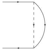
Figure 2: A typical vacuum insertion that vanishes in the LF perturbation theory.

The representation as a correlation function, allows a perturbative expansion using standard Feynman rules. For a free fermion, this reproduces the well known result. Indeed, if one consider $\ln Z_{n}$, then only the connected diagrams will contribute

$$\ln Z_{n}(L)=\sum\text{connected diagrams with insertions of $\int dx\psi^{\dagger}\psi$}\ .$$ (29)

For a free fermion, this means loops with arbitrary numbers of $\bar{\psi}_{k}\gamma^{0}\psi_{k}$ insertions. However, due to the absence of anomalies for any fermion loop with more than three fermion propagators, an application of the vector and axial Ward identities, shows that all loops (with more than three insertions) vanish. The only non-vanishing diagram is the vacuum polarization diagram shown in Fig. 3, at the origin of the 2D axial anomaly. A direct calculation leads to the standard central charge $\frac{N_{c}}{3}$.

More specifically, the vacuum polarization diagram in Fig. 3 contributes as

$$\ln Z_{n}|_{\rm bubble}=\frac{N_{c}}{2}\sum_{k}\bigg{(}\frac{2\pi k}{n}\bigg{)}^{2}\int\frac{d^{2}p}{(2\pi)^{2}}\Pi^{00}(p)\frac{2-2\cos p^{z}L}{(p^{z})^{2}}\ ,$$ (30)

for a massive fermion one has the well known vacuum polarization in $2D$

$$\Pi^{00}(p)=\frac{(p^{z})^{2}}{\pi}\int_{0}^{1}dx\frac{1}{p^{2}+\frac{m^{2}}{x(1-x)}}\ ,$$ (31)

with the result

$$\ln Z_{n}|_{\rm bubble}=-\frac{(n^{2}-1)N_{c}}{12n}\int_{0}^{1}dx\int^{\infty}_{-\infty}dp_{z}\frac{1-\cos p_{z}L}{\sqrt{p_{z}^{2}+\frac{m^{2}}{x(1-x)}}}\ .$$ (32)

The first term diverges in the UV. Using the UV regulator

$$1-\cos p_{z}L\rightarrow\cos p_{z}a-\cos p_{z}L\,,$$

the result is

$$\ln Z_{n}|_{\rm bubble}=-\frac{(n^{2}-1)N_{c}}{6n}\int_{0}^{1}dx\bigg{[}K_{0}\bigg{(}\frac{ma}{\sqrt{x(1-x)}}\bigg{)}-K_{0}\bigg{(}\frac{mL}{\sqrt{x(1-x)}}\bigg{)}\bigg{]}\ ,$$ (33)

with the Renyi entropy (3) in the form

$$S_{n}=\frac{(n+1)N_{c}}{6n}\int_{0}^{1}dx\bigg{[}K_{0}\bigg{(}\frac{ma}{\sqrt{x(1-x)}}\bigg{)}-K_{0}\bigg{(}\frac{mL}{\sqrt{x(1-x)}}\bigg{)}\bigg{]}\rightarrow\frac{N_{c}}{3}{\rm ln}\bigg{(}\frac{L}{a}\bigg{)}$$ (34)

The rightmost result follows in the massless limit ($m\rightarrow 0$), for $n=1$. The L-dependent central charge is

$$c_{n}(L)=L\frac{dS_{n}}{dL}=\frac{(n+1)N_{c}}{6n}\int_{0}^{1}dx\frac{mLK_{1}(\frac{mL}{\sqrt{x(1-x)}})}{\sqrt{x(1-x)}}\ ,$$ (35)

which is seen to decay exponentially as $N_{c}e^{-2mL}$, at large $L$. The Renyi entropy (34) at large $L$, is dominated by the constant UV contribution

$$\frac{(n+1)N_{c}}{6n}\bigg{(}\int_{0}^{1}dxK_{0}\bigg{(}\frac{ma}{\sqrt{x(1-x)}}\bigg{)}+{\cal O}(e^{-2mL})\bigg{)}\rightarrow\frac{(n+1)N_{c}}{6n}\bigg{(}{\rm ln}\bigg{(}\frac{1}{ma}\bigg{)}+{\cal O}(e^{-2mL})\bigg{)}$$

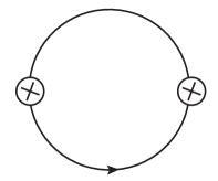
Figure 3: The vacuum polarization contribution to $\ln Z_{n}$ in Eq. (II.2). The crossed dots denote insertions of the operator $\int dx\psi^{\dagger}\psi$. For massless free fermions, it is the only non-vanishing diagram, and contributes t the known $c=\frac{N_{c}}{3}$. For a super-renormalizable theory, this is the only diagram that contains a UV divergence.

Since the interaction is super-renormalizable (valid also for 2D QED), any diagram with interactions vertices will be less singular than the vacuum polarization diagram. In other words, they are UV free, and contribute ${\cal O}\big{(}g^{2n}L^{2n}\big{)}$ at short distances. The dominant contribution at small $L$, is therefore

$$S(L)=\frac{N_{c}}{3}\ln\frac{L}{a}+{\cal O}\big{(}g^{2}L^{2}\big{)}\ .$$ (37)

On the other hand, we expect exponential decay with $L$ at large $L$, for massive fermions.

Finally, we note that for two disjoint intervals, the above formalism allows the calculation of the so-called mutual information,

$$\ln Z_{n}(L_{1}\cup L_{2})-\ln Z_{n}(L_{1})-\ln Z_{n}(L_{2})$$

$$=\sum\text{connected diagrams with both insertions in $L_{1}$ and $L_{2}$ }\ .$$ (38)

Since the distance between $L_{1}$ and $L_{2}$ are non-zero, the diagrams have a natural UV cutoff and will be convergent. This applies even to super-renormalizable theories (Gross-Neveu) after coupling constant renormalization.

III.3 Summing planar contributions with replicas: counting $n-1$

In the large $N_{c}$ limit, the leading contribution is again dominated by a single planar fermion-loop with possible insertions of the charge-operators. We are only interested in the leading $n-1$ contributions that lead to the entanglement entropy. Here we present a power-counting argument that eliminates most of the diagrams.

Notice that the insertions of the $\int dx\psi^{\dagger}\psi$ operators in each of the fermion propagator, have the generic structure

$${\cal G}_{i,j}(p,p^{\prime})=\delta_{ij}G_{0}(p,p^{\prime})+\sum_{m=1}^{\infty}G_{m}(p,p^{\prime})A^{m}_{ij}\ ,$$ (39)

where $p$ and $p^{\prime}$ denotes the incoming and outgoing momenta, and

$$A^{n}_{ij}=\sum_{k=-\frac{n-1}{2}}^{\frac{n-1}{2}}e^{-i\frac{2\pi k}{n}(i-j)}\bigg{(}\frac{k}{n}\bigg{)}^{n}\ ,$$ (40)

is an ij-matrix in replica space, with eigenvalues $(\frac{k}{n})^{n}$. For any diagram, the $n$ dependence follows from the trace over matrices formed by $A$, depending on the locations and numbers of the insertions.

Now consider the generic replica-color structure shown in Figure. 4. Inside a single fermion loop there is a ladder formed by $N$ instantaneous gluons.

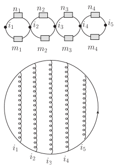
Figure 4: A generic replica-color structure of a planar diagram that contributes to ${\cal O}(N_{c})$. The upper diagram follows by inserting the replica fluxes $(n_{i},m_{i})$ in the lower diagram, in each of the lines between the gluonic exchanges. The dotted 4-Fermi interactions labeled by the replica index $i$ in the upper diagram, is short for the integrated gluon exchange from the lower diagram in 2D.

Let’s now make insertions on the fermion propagators. The number of powers of $A$ on each rung is labelled by $(n_{i},m_{i})$ where $i=0,1,2..N$. Lets show that there exits only a single $i$ in which one of the $(n_{i},m_{i})$ can be non-vanishing. Indeed, one can go from the left side, by summing over $i_{1}$ one obtain

$$A^{n_{1}+m_{1}}_{ii}\propto\sum_{k=-\frac{n-1}{2}}^{\frac{n-1}{2}}\frac{k^{n_{1}+m_{1}}}{n^{n_{1}+m_{1}}}\ ,$$ (41)

which is independent of $i$, and is always proportional to $(n-1)$ as long as $n_{1}+m_{1}\neq 0$. Therefore, if $n_{1}+m_{1}\neq 0$, no other insertions are allowed. Otherwise one obtain $\delta_{i_{1}i_{2}}$ and go to $(n_{2},m_{2})$. Continue this way the assertion is confirmed.

Given the rules above, it is not hard to find the diagrams that are leading in $n-1$. Indeed, a generic planar diagram can be obtained from Fig. 4 by inserting rainbow-like 1PI diagrams, on each of the fermion propagator. If the operator insertions are outside such rainbows, then the replica-color structure remains the same, and the above argument applies. Specifically, for the $i$-ring with the insertion numbers $(n_{i},m_{i})$ possibly non-zero, one may add rainbows between the insertions, without changing the counting in $n-1$. Moreover, if the insertions are inside such rainbows, then by moving the legs of the gluons along the contour, one can view the gluons inside the rainbow, as forming a ladder. The other gluons that used to be a ladder, become rainbows. In this way we are again reduced to the previous case.

III.4 Order ${\cal O}(N_{c})$ contribution

The diagrams that are leading have the topological structure shown in Fig 5.

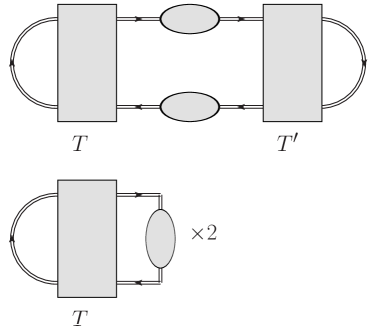
Figure 5: The single-loop contribution. The shaded boxes are the planar two to two amplitudes and the insertions are located at the shaded circles. Notice that between two insertions there can be arbitrary numbers of rainbows.

In the upper diagram above, at least one of $T$ and $T^{\prime}$ is non-trivial. If one of $T$ and $T^{\prime}$ is trivial, then the first diagram reduces to the lower one. However, notice that in these cases the $T$ and $T^{\prime}$ themselves can be viewed as forming rainbows, therefore the above diagrams are really equivalent to the following: arbitrary number of operators inserted in a fermion-loop with arbitrary number equal or grater than $1$ of rainbows inserted along the fermion propagators between them. When combined with the diagram without any rainbow insertions, the fermion propagator between the operator insertions resummes to the dressed one.

With this in mind, the leading $N_{c}$ contribution to the entanglement entropy is actually equivalent to that of a free fermion, but with a rainbow dressed propagator

$$S_{N_{c}}=N_{c}S(\langle\psi(x-y)\bar{\psi}(0)\rangle_{\rm Rainbow})\ ,$$ (42)

Here $S(G_{\rm Rainbow}(x-y))$ denotes the entanglement entropy for a free fermion, with a rainbow dressed propagator Einhorn (1976); Frishman (1979)

$$G_{\rm Rainbow}((x-y))=\int\frac{d^{2}p}{(2\pi)^{2}}e^{-ip(x-y)}\frac{p^{+}\gamma^{+}+(p^{-}+\frac{g^{2}N_{c}}{2\pi p^{+}}-Ag^{2}N_{c}{\rm sign}(p^{+}))\gamma^{-}+m}{p^{2}-m^{2}+\frac{1}{\pi}g^{2}N_{c}-Ag^{2}N_{c}|p^{+}|}$$

with $A$ a gauge parameter.

The fact that (42) through (III.4) depends on $A$, means that in general, the entanglement entropy in a gauge theory, is inherently gauge dependent, even after the elimination of the gauge degrees of freedom in 2D QCD as we discussed earlier. We note that ^′t Hooft originally identified $A=\frac{1}{\epsilon^{-}}$ with an infrared cutoff ’t Hooft (1974), for which its removal from (III.4) will cause the contribution (42) to vanish. However, this is a particular gauge choice. In the $A=0$ gauge (regular cutoff prescription) Einhorn (1976), the rainbow resummation in (III.4) is non-vanishing, with a renormalized squared mass $\tilde{m}^{2}=m^{2}-g^{2}N_{c}/\pi\geq 0$.

Since the gauge dependent part of the self-energy does not change the short distance behavior, the small $L$ behavior of the resummed entanglement entropy, in the planar approximation, is still dominated by the vacuum polarization diagram. It is gauge invariant (independent of $A$), and is equal to $\frac{N_{c}}{3}\ln\frac{L}{a}$. This result is reminiscent of the current-current 2-point function which is given by the free fermion loop and of order $N_{c}$ Callan et al. (1976), an illustration of parton-hadron duality in 2D QCD. For $\tilde{m}^{2}>0$, the asymptotics of the central charge is seen to vanish as $N_{c}e^{-2\tilde{m}L}$, with the Renyi entropy dominated by the constant UV contribution (III.2) at large $L$, which is also gauge independent! These results are unaffected by the ${\cal O}(1)$ contributions as we discuss below.

Finally, we note that the case $m=0$ is pathological with $\tilde{m}^{2}<0$ tachyonic. In this case, the left and right hand fermions decouple, with the fermionic propagator for the right-hand particle unchanged, while for the left particle it changes to

$$G^{+}(z)=e^{-ig^{2}N_{c}A|z|}\gamma^{-}{\rm sign}(z)\int_{0}^{\infty}\frac{dk^{+}}{4\pi}e^{-ik^{+}|z|-i\frac{g^{2}N_{c}-i0}{\pi k^{+}}|z|}\ .$$ (44)

At long distance, (44) decays only polynomially as ${1}/{z^{\frac{3}{2}}}$, and the ensuing entanglement will decay also polynomially. On the other hand, since the right-hand fermion remains free, it will contribute only $\frac{N_{c}}{6}\ln\frac{L}{a}$ at long distances!

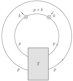
Figure 6: The first non-vanishing double-loop contribution to $Z_{n}$. The shaded box is the amputated two-body planar amplitude. The crossed circles are the insertions of $\psi^{\dagger}\psi$.

III.5 Order ${\cal O}(1)$ contribution

The ${\cal O}(1)$ contributions in the planar approximation, resums the independent mesonic contributions to the entanglement entropy. The meson spectrum contains a would-be Goldstone mode, that may shift the large distance part of the central charge from $\frac{N_{c}}{3}$ to $\frac{N_{c}}{3}+\frac{1}{3}$. We now show that this is not the case.

The ${\cal O}(1)$ contribution is illustrated in Fig. 6. In momentum space, it translates to

$$\ln Z_{n}|_{\rm double}=2\times\frac{1}{2}\sum_{k}\bigg{(}\frac{2\pi k}{n}\bigg{)}^{2}\int\frac{d^{2}k}{(2\pi)^{2}}\tilde{\Pi}^{00}(k)\frac{2-2\cos k^{z}L}{(k^{z})^{2}}\ ,$$ (45)

with $\tilde{\Pi}^{00}(k)$ given by

$$\tilde{\Pi}^{00}(k)=\int\frac{d^{2}p}{(2\pi)^{2}}{\rm tr}S(p)\gamma^{0}S(p+k)\gamma^{0}S(p)\tilde{T}(p)\ ,$$ (46)

and

$$\tilde{T}^{aa^{\prime}}_{\alpha\alpha^{\prime}}(p)=\int\frac{d^{2}\bar{p}}{(2\pi)}T^{aa^{\prime};bb}_{\alpha\alpha^{\prime};\beta\beta^{\prime}}(p,\bar{p})S_{\beta^{\prime}\beta}(\bar{p})\ .$$ (47)

Note that only the forward but off-mass shell part of the $T$ matrix is needed. In light cone gauge, $\tilde{T}$ follows from Fig. 7.

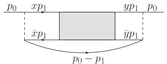
Figure 7: The LF diagram for $\tilde{T}(p_{0}^{+},p_{0}^{-})$ where $p_{0}^{+}$ is positive (it is negative for the flipped antiquark line). The shaded box represents the equal incoming-outgoing LF time $T$ matrix, and the dashed line represents the instantaneous gluon at equal LF time.

To evaluate this, one first notices that the equal incoming-outgoing time $T$ matrix in LF gauge is simply given by

$$T(r^{+},r^{-},x,y)=\frac{g^{2}}{(r^{+})^{2}}\bigg{(}\frac{\pi r^{2}}{g^{2}N_{c}}-\frac{\gamma-1}{x}-\frac{\gamma-1}{\bar{x}}\bigg{)}\delta(x-y)$$

$$-\frac{g^{2}}{(r^{+})^{2}}\bigg{(}\frac{\pi r^{2}}{g^{2}N_{c}}-\frac{\gamma-1}{x}-\frac{\gamma-1}{\bar{x}}\bigg{)}\bigg{(}\frac{\pi r^{2}}{g^{2}N_{c}}-\frac{\gamma-1}{y}-\frac{\gamma-1}{\bar{y}}\bigg{)}G(x,y,r^{2})\ ,$$ (48)

with $\gamma=\pi m^{2}/g^{2}N_{c}$. The incoming $+$ component momenta for the quark and the antiquark, are $xr^{+}$ and $\bar{x}r^{+}$, and the total incoming LF energy are $r^{-}$. The mesonic Green function $G(x,y,r^{2})$ can be written in terms of the ^′t Hooft LF wavefunctions $\phi_{n}(x)$ for mesons with squared masses $m_{n}^{2}/g^{2}N_{c}\sim n\pi$ (large $n$)

$$G(x,y,r^{2})=\sum_{n}\frac{\varphi_{n}(x)\varphi_{n}(y)}{\frac{\pi r^{2}}{g^{2}N_{c}}-\frac{\pi m_{n}^{2}}{g^{2}N_{c}}}\ .$$ (49)

Thus, $\tilde{T}$ can be calculated as

$$\tilde{T}(p_{0})=\frac{(g^{2}N_{c})^{2}}{\pi N_{c}}\sum_{n}\int_{0}^{1}dx\int_{0}^{1}dy\int dp_{1}^{-} \int_{0}^{p_{0}^{+}}\frac{dp_{1}^{+}}{(2\pi)^{2}}\frac{\varphi_{n}(x)\varphi_{n}(y)}{(p_{0}^{+}-xp_{1}^{+})^{2}(p_{0}^{+}-yp_{1}^{+})^{2}}$$

$$\times\frac{(p_{0}-p_{1})^{+}}{(p_{0}-p_{1})^{2}-m^{2}+\frac{g^{2}N_{c}}{\pi}}\frac{(p_{1}^{+})^{2}}{(p_{1})^{2}-m_{n}^{2}}\ .$$ (50)

in the gauge with $A=0$ (regular cut-off prescription). The above integral is convergent at $p_{0}^{+}=p_{1}^{+}$ only if $\varphi_{n}(x)\sim x^{\beta}$ near the edges with $0<\beta<1$. The above can be calculated as

$$p_{0}^{+}\tilde{T}(p_{0})\equiv\tilde{\Sigma}(p_{0}^{2})$$

$$=\frac{(g^{2}N_{c})^{2}}{\pi^{2}N_{c}}\sum_{n}\int_{0}^{1}dxdydz\frac{\varphi_{n}(x)\varphi_{n}(y)}{(1-xz)^{2}(1-yz)^{2}}\frac{z}{p_{0}^{2}-\frac{m_{n}^{2}}{z}-\frac{m^{2}-\frac{g^{2}N_{c}}{\pi}}{1-z}+i0}\ .$$ (51)

This is actually the order ${1}/{N_{c}}$ correction to the quark-self energy. For an estimation, when $m^{2}=0$, there exists zero mass solution to the ’t Hooft equation with $m_{n}=0$, in this case the contribution reads

$$\Sigma(p_{0}^{2})\sim\frac{(g^{2}N_{c})^{2}}{\pi^{2}N_{c}}\int_{0}^{1}dxdydz\frac{\varphi_{0}(x)\varphi_{0}(y)}{(1-xz)^{2}(1-yz)^{2}}\frac{z}{p_{0}^{2}+\frac{\frac{g^{2}N_{c}}{\pi}}{1-z}+i0}\ .$$ (52)

If one use $\phi_{0}=1$, the integral diverges logarithmically near $z=1$. For small but finite $m$, the contribution is of order ${\sqrt{g^{2}N_{c}}}/{m}$. When resummed into the fermion propagator, we have

$$S(p_{0})=\frac{p_{0}^{+}}{p_{0}^{2}-m^{2}+\frac{g^{2}N_{c}}{\pi}+\Sigma(p_{0}^{2})}\ .$$ (53)

in the $A=0$ gauge (regular cutoff prescription). A rerun of the preceding arguments yields a central charge $\frac{N_{c}}{3}$, with no additional $\frac{1}{3}$ contribution from the would-be Golstone mode at long distances.

IV Spatial entanglement in excited states

The present analysis can be generalized to any excited state $|N\rangle$. Using the pertinent interpolating fields to create the excited meson or baryon states, (24) readily generalizes to

$$Z_{N_{n}}(L)=\langle N_{n}|{\cal T}\exp\bigg{[}\sum_{k}i\frac{2\pi k}{n}\int_{0}^{L}dsn^{\mu}\epsilon_{\mu\nu}j^{\nu}_{k}(sn^{\mu})\bigg{]}|N_{n}\rangle\ ,$$ (54)

where $|N_{n}\rangle$ is a tensor product of $|N\rangle$, one for each replica copy,

$$|N_{n}\rangle=\bigotimes_{i=0}^{n-1}|N\rangle_{i}\ .$$ (55)

Moreover, if we choose $n^{\mu}$ to be along the LF^- direction, then (54) is reminiscent of LF parton distribution functions.

IV.1 Free parton on the light front

For a free fermion state of longitudinal momentum $P^{+}$ or $|N\rangle=b_{P^{+}}^{\dagger}|\Omega\rangle$, the contributions for different $k$ factorize,

$$\ln Z_{n}=(1-n)S_{n}+\sum_{k=-\frac{n-1}{2}}^{\frac{n-1}{2}}\ln\bigg{[}\int^{\Lambda^{-}/2}_{-\Lambda^{-}/2}\frac{dxdy}{2\pi\Lambda^{-}}\frac{ie^{-i(x-y)}}{x-y+i0}\bigg{(}\frac{(x-\lambda+i0)(y-i0)}{(y-\lambda-i0)(x+i0)}\bigg{)}^{\frac{k}{n}}\bigg{]}\ .$$ (56)

Here $R^{-}$ is the box size along LF^-, and $\Lambda^{-}=P^{+}R^{-}$ and $\lambda=P^{+}L^{-}$ the invariant lengths. In deriving (56), we used the bosonized representation for the fermion field $\psi_{k}\sim e^{i\phi_{k}}$ in (54). In the large LF box limit with $L^{-}/R^{-}\ll 1$, the kernel in (56) can be reduced,

$$\ln Z_{n}-(1-n)S_{n}=-\frac{4\lambda}{\Lambda^{-}}\sum_{k=-\frac{n-1}{2}}^{\frac{n-1}{2}}\sin^{2}\frac{k\pi}{n}\int_{0}^{1}\frac{dxdy}{2\pi}\bigg{[}\frac{(1-x)y}{(1-y)x}\bigg{]}^{\frac{k}{n}}\frac{\sin\lambda(x-y)}{x-y}\ .$$ (57)

The details are in Appendix A. The entanglement entropy follows by performing the $n\rightarrow 1$ limit in (57), using the formula Casini et al. (2005)

$$\lim_{n\rightarrow 1}\frac{1}{1-n}\sum_{k=-\frac{n-1}{2}}^{\frac{n-1}{2}}\sin^{2}\frac{k\pi}{n}z^{\frac{k}{n}}\sim-\lim_{n\rightarrow 1}\frac{2\pi^{2}(n-1)}{4\pi^{2}(n-1)^{2}+(z-1)^{2}}=-\pi^{2}\delta(z-1)\ ,$$ (58)

with the result

$$S=S(L^{-})+\frac{4\pi^{2}\lambda}{\Lambda^{-}}\int_{0}^{1}\frac{dxdy}{2\pi}\delta(x-y)y(1-y)\frac{\sin\lambda(x-y)}{x-y}=S(L^{-})+\frac{\pi\lambda^{2}}{3\Lambda^{-}}\ .$$ (59)

$S(L^{-})$ is the vacuum entanglement entropy discussed earlier. For large LF^- intervals with invariant length $\lambda=P^{+}L^{-}$, the entanglement entropy of a free fermion on the LF is of order $\frac{\lambda^{2}}{\Lambda^{-}}$. For small intervals, it is dominated by the Logarithmic contribution from the vacuum in $S(L^{-})$. In particular, for a free fermionic parton with the least longitudinal momentum $P^{+}=\frac{2\pi}{R^{-}}$, (59) simplifies to

$$S=S(L^{-})+\frac{2\pi^{2}}{3}\bigg{(}\frac{L^{-}}{R^{-}}\bigg{)}^{2}\,.$$ (60)

The additional contribution is the entanglement entropy for a primary state in a free conformal field theory Berganza et al. (2012) with $h=1$ and $\bar{h}=0$.

IV.2 Free meson on the light front

Consider a bound meson state on the LF, with longitudinal momentum $P^{+}$,

$$|l\rangle=B_{l,P^{+}}^{\dagger}|\Omega\rangle\equiv\frac{1}{(\Lambda^{-})^{\frac{1}{2}}}\int d\lambda_{1}d\lambda_{2}\varphi_{l}(\lambda_{1},\lambda_{2})\psi^{\dagger}(\lambda_{1})\psi(\lambda_{2})|\Omega\rangle\ ,$$ (61)

with the coordinate space light-front wave function (LFWF)

$$\varphi_{l}(\lambda_{1},\lambda_{2})=\frac{1}{(2\pi)^{2}}\int_{0}^{1}dxe^{-i\lambda_{1}x-i\lambda_{2}(1-x)}\varphi_{l}(x)\ .$$ (62)

and the normalization $\int dx|\varphi_{l}(x)|^{2}=1$. In the replica states constructed from (61), the replica partition function is

$$Z_{n}(l)=\langle\Omega|\prod_{j=0}^{n-1}B_{l,j}\exp\bigg{[}\sum_{k}i\frac{2\pi k}{n}\int_{0}^{\lambda}d\lambda^{\prime}\psi_{k}^{\dagger}(\lambda^{\prime})\psi_{k}(\lambda^{\prime})\bigg{]}\prod_{j^{\prime}=0}^{n-1}B_{l,j^{\prime}}^{\dagger}|\Omega\rangle\ .$$ (63)

The correponding entanglement entropy to leading order in $1/\Lambda^{-}$, is of the form (59). More specifically, it is proportional to $\lambda^{2}$, but dressed but the second moments of the quark/antiquark PDFs

$$S=S(L^{-})+\frac{\pi\lambda^{2}}{3\Lambda^{-}}\big{(}\langle x_{q}^{2}\rangle_{l}+\langle x_{\bar{q}}^{2}\rangle_{l}\big{)}+{\cal O}\bigg{(}\frac{1}{\Lambda^{-2}}\bigg{)}\ ,$$ (64)

where

$$\langle x_{q}^{2}\rangle_{l}=\int_{0}^{1}dx\,x^{2}\,|\varphi_{l}(x)|^{2}\ ,\qquad\qquad\langle x_{\bar{q}}^{2}\rangle_{l}=\int_{0}^{1}dx\,\bar{x}^{2}\,|\varphi_{l}(x)|^{2}\ ,$$ (65)

are the second moments of the quark and antiquark PDFs. The higher and even moments of the PDFs are suppressed by further powers of $1/\Lambda^{-}$, in the entanglement entropy (64). For the meson state in the Schwinger model, each of the second moment is $\frac{1}{3}$.

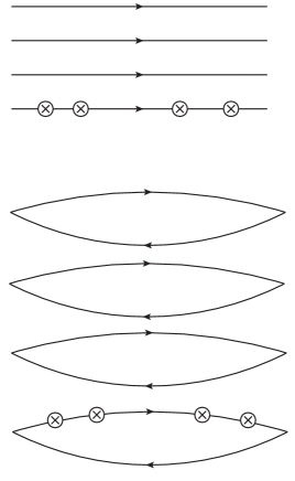
Figure 8: The leading ${1}/{\Lambda^{-}}$ contribution to the spatial entanglement for n-replicated fermion (upper) and n-replicated meson states (lower). The crossed circles denote the vector current operator insertions. To leading order in ${1}/{\Lambda^{-}}$, $n-1$ pairs of the replicated external states contract with themselves, leaving only one pair for the vector current insertion. To leading order in $n-1$, no additional insertion is needed.

To derive (64), it is best to use a diagrammatic analysis of (63) as illustrated in Fig. 8. The disconnected bubbles where the meson operators contract among themselves, exponentiate and contribute to the vacuum state entanglement. So we need to consider only the connected diagrams where the combination $\psi_{i}^{\dagger}\psi_{i}$ from the external state, contracts with $\psi_{k}^{\dagger}\psi_{k}$ from the vector operator in the exponent. We now note that each time a $\psi_{i}^{\dagger}\psi_{i}$ from the external state contracts with $\psi_{k}^{\dagger}\psi_{k}$ from the operator insertion, a suppression factor ${1}/{\Lambda^{-}}$ arises. Hence, the leading ${1}/{\Lambda^{-}}$ contribution consists of $n-1$ pairs of external state contracted among themselves, with the remaining pair contracted with $\psi_{k}^{\dagger}\psi_{k}$ from the vector operator insertion.

For a replicated fermion in Fig. 8 (top), this contribution is the trace over the $i$-fields, which readily converts to the sum over the k-fields. This reproduces the second term in 86. The extra $-1$ corresponds to the subtraction of the term with no insertions.

This observation extends to the replicated meson state as well. The leading contribution is shown in Fig. 8 (bottom). For a generic $n$, the operators can be inserted simultaneously on the fermion/antifermion lines. To obtain the linear contribution in $n-1$, one needs the insertions exclusively on either the fermion, or the antifermion legs, but not both. In this case one reproduces the above free fermion contributions, but weighted over the LFWF of the meson,

$$S-S(L^{-})=\frac{1}{\Lambda^{-}}\int_{0}^{1}dx|\varphi_{n}(x)|^{2}\bigg{(}F_{\rm single}(x\lambda)+F_{\rm single}(\bar{x}\lambda)\bigg{)}\ ,$$ (66)

where $F_{\rm single}(\lambda)=\frac{\lambda^{2}\pi}{3}$ is the fermion contribution. This is (64), and concludes our derivation. One should mention that although the above derivation is for a free replicated meson state, it can be extended to 2D QCD, using the large $N_{c}$ power-counting methods detailed above.

We note that for space-like cuts, the replica partition function (63) can be regarded as a meson-meson correlation function, with replicated fermionic vector charge insertions. In the limit where the meson sources are asymptotically separated, it is in general a function of the form $Z_{n}(P\cdot L,P\cdot R,L^{2},R^{2})$, and can be probed on an Euclidean lattice in the same spirit as the quasi-PDF approach in Ji (2013, 2014), for parton densities. For say large $P^{z}$ and fixed spatial cut $L^{z}<R^{z}={}^{4}\sqrt{V_{4}}$, the second moment of the quark PDF in a meson state can be read from the coefficient of the Renyi entropy that scales like $1/P^{z}R^{z}$.

IV.3 Coherent meson state on the light front

In a general bosonic coherent state

$$|\xi\rangle=e^{-\frac{|\xi^{2}|}{2}-\xi B_{l}^{\dagger}}|\Omega\rangle$$

constructed using (61) with $\xi$ complex valued, the replica partition function is

$$Z_{n}(\xi)=\prod_{k}Z_{k}(\xi)=\prod_{k}e^{-|\xi^{2}|}\langle\Omega|\exp[-\xi^{*}B_{l}]\exp\bigg{[}i\frac{2\pi k}{n}\int_{0}^{\lambda}d\lambda^{\prime}\psi^{\dagger}(\lambda^{\prime})\psi(\lambda^{\prime})\bigg{]}\exp[-\xi B_{l}^{\dagger}]|\Omega\rangle\ .$$ (67)

For 2D QCD the reduction of (67) in terms of the LFWF $\varphi_{l}(x)$ is straightforward, but tedious. This construction maybe used to probe for many-body correlations. (67) simplifies considerably for 2D QED or the Schwinger model. Indeed, for the latter $B_{l}$ is nothing but the bosonized field, and (67) can be reduced by bosonization to

$$\ln Z_{k}(\xi)=\ln Z_{k}-\frac{2\xi k}{n}\frac{\sqrt{2\pi}}{\sqrt{P^{+}L^{-}}}\sin\lambda\ .$$ (68)

where $Z_{k}$ is the vacuum contribution. After summing over $k$, all the $k$ dependent terms cancel out, with only the vacuum contribution remaining. For the Schwinger model, the bosonic coherent state has the same LF-spatial entanglement as that of the vacuum.

V Holographic dual construction

In this section, we will construct a soft wall holographic dual to two-dimensional QCD, using the bottom up approach. Using the Ryu-Takayanagi proposal Ryu and Takayanagi (2006), we will derive the entanglement entropy geometrically. We will illustrate the derivation, by recalling the construction for two-dimensional CFT with an AdS₃ gravity dual, and then extend it to the non-conformal case of two-dimensional QCD using soft-wall AdS₃.

V.1 AdS₃

Two-dimensional conformal theories map onto AdS₃, with a central charge $c=3R/2G_{3}$, with $R$ the radius of AdS₃, and $G_{3}$ the bulk Newton gravitational constant. In this regime, the entanglement entropy for the single spatial cut $L=|a_{1}-a_{2}|$, can be read in bulk using the Ryu-Takayanagi proposal Ryu and Takayanagi (2006)

$$S=\frac{\gamma_{L}}{4G_{3}}\rightarrow\frac{c}{3}\,{\rm log}\bigg{(}\frac{R}{a}{\rm sin}\bigg{(}\frac{\pi L}{R}\bigg{)}\bigg{)}$$ (69)

with $\gamma_{L}$ the length of the bulk AdS₃ geodesic. In two dimensions $G_{3}=g_{s}l_{s}$ and $R/G_{3}=(R/l_{s})/g_{s}$, with the string length $l_{s}$. The string coupling is $g_{s}\sim 1/N_{c}$, with the $1/N_{c}$ universal from the genus expansion. For conformal fermions in the fundamental representation, we expect $R/l_{s}=\#>1$ (below # is of order 1), with $c=N_{c}$.

In Poincare coordinates with line element

$$ds^{2}=\frac{R^{2}}{z^{2}}\bigg{(}-dt^{2}+dx^{2}+dz^{2}\bigg{)}$$ (70)

the geodesic is a semi-circle ${\dot{x}}^{2}+{\dot{z}}^{2}=(L/2)^{2}$,

$$(x(s),z(s))=\frac{L}{2}({\rm cos}\,s,{\rm sin}\,s)$$ (71)

sustained by the single-cut end-points $\pm L/2$, on the Minkowski boundary at $z=a\ll L$ (range $2a/L\leq s\leq\pi-2a/L$). The geometric entanglement entropy is the length of the geodesic in Planck units

$$S=\frac{1}{4G_{3}}\int_{2a/L}^{\pi/2}\,ds\,\sqrt{g_{MN}{\dot{x}}^{M}{\dot{x}}^{N}}=\frac{R}{2G_{3}}\int_{2a/L}^{\pi/2}\,\frac{ds}{\rm sin\,s}=\frac{R}{2G_{3}}{\rm log}\bigg{(}\frac{\pi L}{a}\bigg{)}$$ (72)

Figure 9: $F(\tilde{z}_{m})$ in (81) as a function of $\tilde{z}_{m}$, with a maximum at $\tilde{z}_{m}\sim 1.4$.

V.2 Soft-wall AdS₃

Assuming now the geometry is controlled by a soft-wall AdS₃

$$ds^{2}=\frac{e^{-\kappa^{2}z^{2}}}{z^{2}}(dz^{2}+dx^{2}-dt^{2})\ ,$$ (73)

where $\kappa^{2}\propto g^{2}N_{c}$ plays the role of the “string tension”. The minimal surface is parameterized by

$$(x,z,t)=(x(s),z(s),0)\ ,$$ (74)

where $0\leq s\leq 1$. The 2-dimensional bulk action is

$$S=\int ds\frac{e^{\frac{-\kappa^{2}z^{2}}{2}}}{z}\sqrt{\dot{x}^{2}+\dot{z}^{2}}\ ,$$ (75)

for which the minimal surface can be chosen to satisfy

$$\frac{\dot{x}}{\sqrt{\dot{x}^{2}+\dot{z}^{2}}}\frac{e^{-\frac{\kappa^{2}z^{2}}{2}}}{z}=\alpha\ ,$$ (76)

$$\dot{x}^{2}+\dot{z}^{2}=\beta^{2}\ ,$$ (77)

which leads to

$$\dot{z}^{2}=\alpha^{2}\beta^{2}(z_{m}^{2}e^{\kappa^{2}z_{m}^{2}}-z^{2}e^{\kappa^{2}z^{2}})\ ,$$ (78)

$$\dot{x}=\alpha\beta ze^{\frac{\kappa^{2}}{2}}\ ,$$ (79)

Here $z_{m}$ is the maximal value of $z$ attained at $s=\frac{1}{2}$, which satisfies

$$\frac{L}{2}=\int_{0}^{1}ds\dot{x}=\int_{0}^{z_{m}}dz\frac{ze^{\frac{\kappa^{2}z^{2}}{2}}}{\sqrt{z_{m}^{2}e^{\kappa^{2}z_{m}^{2}}-z^{2}e^{\kappa^{2}z^{2}}}}\ .$$ (80)

For small $L$ (80) reproduces the circular solution in AdS₃ discussed above. For large $L$, we define $\tilde{z}_{m}=z_{m}\kappa$ and $\tilde{L}=L\kappa$ , so that

$$\frac{\tilde{L}}{2}=\tilde{z}_{m}\int_{0}^{1}dt\frac{t}{\sqrt{e^{\tilde{z}_{m}^{2}(1-t^{2})}-t^{2}}}\equiv F(\tilde{z}_{m}).$$ (81)

For small $\tilde{z}_{m}\ll 1$, $F(\tilde{z}_{m})=\tilde{z}_{m}$ and the circular solution follows. However, a maximum develops for $\tilde{z}_{m}\sim 1.4$, so that $F(\tilde{z}_{m})\leq 0.72$. The connected solutions only exist for small $L$, at strong ’t Hooft coupling

$$L\leq\frac{1.44}{\kappa}\sim\frac{1.44}{\sqrt{g^{2}N_{c}}}\ .$$ (82)

For large $L$ the minimal surface cannot be smoothly connected to the small $L$ solution. A similar observation was also made for D-branes in higher dimensions, where at large $L$ the solution was argued to be made of two disjoints in-falling geodesics Klebanov et al. (2008). For the soft-wall model, this disconnected geometry can be approximated by

$$S\approx 2\times\frac{R}{4G_{3}}\int_{a}^{z_{m}}\frac{dz}{z}=\frac{R}{2G_{3}}{\rm log}\bigg{(}\frac{z_{m}}{a}\bigg{)}$$ (83)

The net entanglement entropy is a competition between the circular (72) and disjoint (83) geometries,

$$\Delta S=S(\kappa L\ll 1)-S(\kappa L\gg 1)=\frac{R}{2G_{3}}{\rm log}\bigg{(}\frac{\pi L}{z_{m}}\bigg{)}\rightarrow\frac{N_{c}}{3}\,{\rm log}\bigg{(}\frac{\pi L}{z_{m}}\bigg{)}$$ (84)

The Ryu-Takayanagi entropies for small (72) and large (83) spatial cuts, are in agreement with the perturbative Renyi entropy (III.2), and its non-perturbative analogue $m\rightarrow\tilde{m}$ at large $N_{c}$, respectively.

This interpolation between a connected surface for small cuts, and a disconnected surface for large cuts is similar to the observation put forth in Klebanov et al. (2008), for several holographic constructions dual to 4D conformal and confining gauge theories. However, the chief difference in our case stems from the fact that 2D QCD at large $N_{c}$, confines at all distance scales. The geometrical change we observed, is not related to a Hagedorn-like growth in the confined meson spectrum as argued in 4D QCD in Klebanov et al. (2008), as there is none in 2D, but is rather a reflection of parton-hadron duality for small intervals in 2D QCD.

VI Conclusions

We have shown how to extend the replica construction to Minkowski space-time signature, and use it to derive a general formula for the replica partition function in the vacuum state. Our result applies to a large class of interacting theories with fermions with or without gauge fields, for any space-time cut and in arbitrary dimensions. When analytically continued to Euclidean signature, our result can be explicitly reduced to the standard result, using bosonization.

In the presence of gauge interactions, spatial entanglement as described by our replica partition function, is in general gauge dependent, a result of gluing fermionic fields valued in different replica strips along the spatial cut. However, the ensuing Renyi entropy for small or large cuts can still exhibit gauge independent contributions. We have shown that this is the case in two-dimensional QCD.

For small space-like cuts, the Renyi entropy was shown to follow from the charge density correlation function, which is fixed at short distance by the 2D axial anomaly. The central charge is $\frac{N_{c}}{3}$ and gauge independent. At large distances, the perturbative arguments break down. Using the planar expansion, we showed that the leading ${\cal O}(N_{c})$ contribution is tied to the rainbow dressed quark propagator, which is explicitly gauge fixing dependent. However, for large cuts, this contribution vanishes exponentially with the distance $L$, leaving behind only the gauge independent UV constant contribution. The mesonic ${\cal O}(1)$ contributions do not change this result.

Our results are not limited to the vacuum state. We have shown that spatial entanglement on the light front can be extended to any hadron state, with minimal changes to our central result for the replica partition function. The result is reminiscent of LF wavefunctions, which shows a direct relationship between the Renyi entropy of an excited hadron, and its parton distribution on the light front. Conversely and for space-like intervals, the even moments of the quark PDFs in a hadron state in 2D QCD, can be extracted from the Renyi entropy at large momentum. This observation extends to 4D QCD both in the continuum, and on an Euclidean lattice.

Using a bottom-up soft-wall model for 2D QCD in AdS₃, we have shown that the Ryu-Takayanagi geometrical entropy, interpolates between the known conformal AdS₃ result for a small spatial cut, and a constant but UV sensitive result for a large spatial cut. This result is in total agreement with the Renyi entropy, following from our new replica construction. Although 2D QCD at large $N_{c}$, is not conformal at all distance scales, the agreement with the conformal AdS₃ result for small intervals, illustrates the parton-hadron duality at work in theories with confinement.

Acknowledgements

This work is supported by the Office of Science, U.S. Department of Energy under Contract No. DE-FG-88ER40388, and by the Priority Research Area SciMat under the program Excellence Initiative - Research University at the Jagiellonian University in Kraków.

Appendix A Details in the kernel reduction

In the large $\Lambda^{-}$ limit one can split the kernel (56) into

$$\int^{\Lambda^{-}/2}_{-\Lambda^{-}/2}\frac{dxdy}{2\pi\Lambda^{-}}\frac{ie^{-i(x-y)}}{x-y+i0}\frac{(x-\lambda+i0)(y-i0)}{(y-\lambda-i0)(x+i0)}\bigg{)}^{\frac{k}{n}}$$

$$=1+\frac{1}{\Lambda^{-}}\int^{\Lambda^{-}/2}_{-\Lambda^{-}/2}\frac{dxdy}{2\pi}\frac{ie^{-i(x-y)}}{x-y+i0}\bigg{[}\bigg{(}\frac{(x-\lambda+i0)(y-i0)}{(y-\lambda-i0)(x+i0)}\bigg{)}^{\frac{k}{n}}-1\bigg{]}\ ,$$ (85)

and

$$\ln Z_{n}=(1-n)S_{n}+\frac{1}{\Lambda^{-}}\sum_{k=-\frac{n-1}{2}}^{\frac{n-1}{2}}\int^{\Lambda^{-}/2}_{-\Lambda^{-}/2}\frac{dxdy}{2\pi}\frac{ie^{-i(x-y)}}{x-y+i0}\bigg{[}\bigg{(}\frac{(x-\lambda+i0)(y-i0)}{(y-\lambda-i0)(x+i0)}\bigg{)}^{\frac{k}{n}}-1\bigg{]}\ .$$ (86)

The reduction of (86) follows by noting that the bracket is of the form

$$F(z)=\ln(z-\lambda)-\ln z\ ,$$ (87)

with a branch cut along $[0,\lambda]$ with discontinuity $2\pi i$. The ensuing integral follows by contour

$$\int^{\Lambda^{-}/2}_{-\Lambda^{-}/2}\frac{dxdy}{2\pi}\frac{ie^{-i(x-y)}}{x-y+i0}\bigg{[}\bigg{(}\frac{(x-\lambda+i0)(y-i0)}{(y-\lambda-i0)(x+i0)}\bigg{)}^{\frac{k}{n}}-1\bigg{]}$$

$$=\int^{\Lambda^{-}/2}_{-\Lambda^{-}/2}\frac{dxdy}{2\pi}\frac{ie^{-i(x-y)}}{x-y+i0}e^{\frac{k}{n}F(x+i0)-\frac{k}{n}F(y-i0)}$$

$$=\int^{\Lambda^{-}/2}_{-\Lambda^{-}/2}\frac{dxdy}{2\pi}\frac{ie^{-i(x-y)}}{x-y+i0}\bigg{[}e^{\frac{k}{n}F(x-i0)-\frac{k}{n}F(y-i0)}+\delta A(x)e^{-\frac{k}{n}F(y-i0)}\bigg{]}$$

$$=\Lambda^{-}+\int^{\Lambda^{-}/2}_{-\Lambda^{-}/2}\frac{dxdy}{2\pi}\frac{ie^{-i(x-y)}}{x-y+i0}\delta A(x)e^{-\frac{k}{n}F(y-i0)}$$

$$=\Lambda^{-}+\int^{\Lambda^{-}/2}_{-\Lambda^{-}/2}\frac{dxdy}{2\pi}\frac{ie^{-i(x-y)}}{x-y+i0}\delta A(x)\delta B(y)+\int^{\Lambda^{-}/2}_{-\Lambda^{-}/2}dx\delta A(x)e^{-\frac{k}{n}F(x+i0)}\ ,$$ (88)

with

$$\delta A(x)=e^{\frac{k}{n}F(x-i0)}-e^{\frac{k}{n}F(x+i0)}=(e^{-\frac{2\pi k}{n}i}-1)e^{\frac{k}{n}F(x+i0)}\theta(x)\theta(\lambda-x)\ ,$$ (89)

$$\delta B(y)=e^{-\frac{k}{n}F(y+i0)}-e^{-\frac{k}{n}F(y-i0)}=(1-e^{\frac{2\pi k}{n}i})e^{-\frac{k}{n}F(y+i0)}\theta(y)\theta(\lambda-y)\ .$$ (90)

Using the PP-assignment $\frac{1}{x-y+i0}={\rm PV}.\frac{1}{x-y}-i\pi\delta(x-y)$, we obtain (57).

References

- Srednicki (1993) Mark Srednicki, “Entropy and area,” Phys. Rev. Lett. 71, 666–669 (1993), arXiv:hep-th/9303048 .
- Calabrese and Cardy (2004) Pasquale Calabrese and John L. Cardy, “Entanglement entropy and quantum field theory,” J. Stat. Mech. 0406, P06002 (2004), arXiv:hep-th/0405152 .
- Casini et al. (2005) H. Casini, C. D. Fosco, and M. Huerta, “Entanglement and alpha entropies for a massive Dirac field in two dimensions,” J. Stat. Mech. 0507, P07007 (2005), arXiv:cond-mat/0505563 .
- Hastings (2007) M. B. Hastings, “An area law for one-dimensional quantum systems,” J. Stat. Mech. 0708, P08024 (2007), arXiv:0705.2024 [quant-ph] .
- Calabrese and Cardy (2009) Pasquale Calabrese and John Cardy, “Entanglement entropy and conformal field theory,” J. Phys. A 42, 504005 (2009), arXiv:0905.4013 [cond-mat.stat-mech] .
- Bremermann (1967) H.J. Bremermann, in Proceedings of the Fifth Berkeley Symposium on Mathematical Statistics and Probability, Eds. Le Cam, Lucien Marie and Neyman, Jerzy, Vol. 3 (Univ of California Press, 1967).
- Bekenstein (1981) Jacob D. Bekenstein, “Energy Cost of Information Transfer,” Phys. Rev. Lett. 46, 623–626 (1981).
- Kaufman et al. (2016) Adam M Kaufman, M Eric Tai, Alexander Lukin, Matthew Rispoli, Robert Schittko, Philipp M Preiss, and Markus Greiner, “Quantum thermalization through entanglement in an isolated many-body system,” Science 353, 794–800 (2016).
- Stoffers and Zahed (2013) Alexander Stoffers and Ismail Zahed, “Holographic Pomeron and Entropy,” Phys. Rev. D 88, 025038 (2013), arXiv:1211.3077 [nucl-th] .
- Qian and Zahed (2015a) Yachao Qian and Ismail Zahed, “Stretched string with self-interaction at the Hagedorn point: Spatial sizes and black holes,” Phys. Rev. D 92, 105001 (2015a), arXiv:1508.03760 [hep-ph] .
- Berges et al. (2019) Jürgen Berges, Stefan Floerchinger, and Raju Venugopalan, “Entanglement and thermalization,” Nucl. Phys. A 982, 819–822 (2019), arXiv:1812.08120 [hep-th] .
- Florio and Kharzeev (2021) Adrien Florio and Dmitri E. Kharzeev, “Gibbs entropy from entanglement in electric quenches,” Phys. Rev. D 104, 056021 (2021), arXiv:2106.00838 [hep-th] .
- Liu et al. (2022a) Yizhuang Liu, Maciej A. Nowak, and Ismail Zahed, “Entanglement entropy and flow in two dimensional QCD:parton and string duality,” (2022a), arXiv:2202.02612 [hep-ph] .
- Kharzeev and Levin (2017) Dmitri E. Kharzeev and Eugene M. Levin, “Deep inelastic scattering as a probe of entanglement,” Phys. Rev. D 95, 114008 (2017), arXiv:1702.03489 [hep-ph] .
- Liu et al. (2022b) Yizhuang Liu, Maciej A. Nowak, and Ismail Zahed, “Rapidity evolution of the entanglement entropy in quarkonium: parton and string duality,” (2022b), arXiv:2203.00739 [hep-ph] .
- Qian and Zahed (2015b) Yachao Qian and Ismail Zahed, “Stretched String with Self-Interaction at High Resolution: Spatial Sizes and Saturation,” Phys. Rev. D 91, 125032 (2015b), arXiv:1411.3653 [hep-ph] .
- Shuryak and Zahed (2018) Edward Shuryak and Ismail Zahed, “Regimes of the Pomeron and its Intrinsic Entropy,” Annals Phys. 396, 1–17 (2018), arXiv:1707.01885 [hep-ph] .
- Liu and Zahed (2019) Yizhuang Liu and Ismail Zahed, “Entanglement in Regge scattering using the AdS/CFT correspondence,” Phys. Rev. D 100, 046005 (2019), arXiv:1803.09157 [hep-ph] .
- Armesto et al. (2019) Nestor Armesto, Fabio Dominguez, Alex Kovner, Michael Lublinsky, and Vladimir Skokov, “The Color Glass Condensate density matrix: Lindblad evolution, entanglement entropy and Wigner functional,” JHEP 05, 025 (2019), arXiv:1901.08080 [hep-ph] .
- Dvali and Venugopalan (2021) Gia Dvali and Raju Venugopalan, “Classicalization and unitarization of wee partons in QCD and Gravity: The CGC-Black Hole correspondence,” (2021), arXiv:2106.11989 [hep-th] .
- ’t Hooft (1974) Gerard ’t Hooft, “A Two-Dimensional Model for Mesons,” Nucl. Phys. B 75, 461–470 (1974).
- Bars (1976) I. Bars, “A Quantum String Theory of Hadrons and Its Relation to Quantum Chromodynamics in Two-Dimensions,” Nucl. Phys. B 111, 413–440 (1976).
- Ryu and Takayanagi (2006) Shinsei Ryu and Tadashi Takayanagi, “Holographic derivation of entanglement entropy from AdS/CFT,” Phys. Rev. Lett. 96, 181602 (2006), arXiv:hep-th/0603001 .
- Goykhman (2015) Mikhail Goykhman, “Entanglement entropy in ’t Hooft model,” Phys. Rev. D 92, 025048 (2015), arXiv:1501.07590 [hep-th] .
- Armoni et al. (2001) A. Armoni, Y. Frishman, and J. Sonnenschein, “Massless QCD(2) from current constituents,” Nucl. Phys. B 596, 459–470 (2001), arXiv:hep-th/0011043 .
- Einhorn (1976) Martin B. Einhorn, “Form-Factors and Deep Inelastic Scattering in Two-Dimensional Quantum Chromodynamics,” Phys. Rev. D 14, 3451 (1976).
- Frishman (1979) Y. Frishman, “Nonabelian Gauge Theory in Two-Dimensions,” Nucl. Phys. B 148, 74–92 (1979).
- Callan et al. (1976) Curtis G. Callan, Jr., Nigel Coote, and David J. Gross, “Two-Dimensional Yang-Mills Theory: A Model of Quark Confinement,” Phys. Rev. D 13, 1649 (1976).
- Berganza et al. (2012) Miguel Ibanez Berganza, Francisco Castilho Alcaraz, and German Sierra, “Entanglement of excited states in critical spin chians,” J. Stat. Mech. 1201, P01016 (2012), arXiv:1109.5673 [cond-mat.stat-mech] .
- Ji (2013) Xiangdong Ji, “Parton Physics on a Euclidean Lattice,” Phys. Rev. Lett. 110, 262002 (2013), arXiv:1305.1539 [hep-ph] .
- Ji (2014) Xiangdong Ji, “Parton Physics from Large-Momentum Effective Field Theory,” Sci. China Phys. Mech. Astron. 57, 1407–1412 (2014), arXiv:1404.6680 [hep-ph] .
- Klebanov et al. (2008) Igor R. Klebanov, David Kutasov, and Arvind Murugan, “Entanglement as a probe of confinement,” Nucl. Phys. B 796, 274–293 (2008), arXiv:0709.2140 [hep-th] .