Background Effective Action with Nonlinear Massive Gauge Fixing

Abstract

We combine a recent construction of a BRST-invariant, nonlinear massive gauge fixing with the background field formalism. The resulting generating functional preserves background-field invariance as well as BRST invariance of the quantum field manifestly. The construction features BRST-invariant mass parameters for the quantum gauge and ghost fields.

The formalism employs a background Nakanishi-Lautrup field which is part of the nonlinear gauge-fixing sector and thus should not affect observables. We verify this expectation by computing the one-loop effective action and the corresponding beta function of the gauge coupling as an example. The corresponding Schwinger functional generating connected correlation functions acquires additional one-particle reducible terms that vanish on shell. We also study off-shell one-loop contributions in order to explore the consequences of a nonlinear gauge fixing scheme involving a background Nakanishi-Lautrup field.

As an application, we show that our formalism straightforwardly accommodates nonperturbative information about propagators in the Landau gauge in the form of the so-called decoupling solution. Using this nonperturbative input, we find evidence for the formation of a gluon condensate for sufficiently large coupling, whose scale is set by the BRST-invariant gluon mass parameter.

I Introduction

Background fields represent a useful, in some cases essential tool in quantum field theory. Background fields can be chosen to represent a specific physical environment of interest. In continuum gauge theories, the virtue of background fields is that a necessary gauge fixing can be performed such that the generating functionals remain manifestly invariant under gauge transformations of the background field. For suitably chosen gauges, even the full generating functional, e.g., in the form of the effective action for the quantum expectation values, inherits this symmetry property from the background field [1, 2].

Another elegant method to deal with gauge symmetry in continuum gauge-fixed computations is based on BRST symmetry, a residual global supersymmetry that acts nonlinearly on the gauge and auxiliary degrees of freedom [3, 4, 5]. BRST symmetry allows to formulate the constraints for correlation functions imposed by gauge invariance in a closed form given by the Zinn-Justin master equation [6, 7]. As a significant advantage, the latter can be addressed algebraically with the aid of cohomology methods.

Although a continuum Faddeev-Popov formulation of gauge theories, featuring background-gauge and BRST invariance, has proved extremely useful, especially for scattering amplitude computations, it still faces the open challenge of allowing for computations of more general physical observable properties such as for instance a mass spectrum. These difficulties are notoriously related to the phenomena of mass generation and of confinement. Setting aside nonperturbative issues such as the Gribov problem or the Neuberger-zero problem, recent studies have argued that effective Lagrangians very similar to those appearing in the Faddeev-Popov method, namely the Curci-Ferrari massive deformation thereof, are suprisingly accurate as phenomenological tools for the description of such phenomena [8, 9, 10, 11, 12, 13, 14]. Unfortunately, these effective models do not feature a nilpotent BRST symmetry allowing for a cohomological construction of unitarity-preserving physical Hilbert spaces. These studies motivate a renewed interest in the open problem of constructing BRST invariant gauge-fixed Lagrangians featuring mass parameters for all fields.

In a recent work [15], a class of these BRST-invariant massive models has been constructed, together with a renormalization group (RG) flow equation that offers a route to preserving exact BRST symmetry also for nonperturbative approximation schemes. In this way, technical challenges posed by other formulations of RG flows based on momentum-space regularizations can be overcome [16, 17, 18, 19, 20, 21, 22, 23, 24, 25, 26, 27].

The main idea of this construction is to combine Faddeev-Popov quantization with a nonlinear gauge condition in such a way that the regularization procedure (i.e. the mass terms) becomes part of the gauge-fixing sector. Additionally, the construction goes along with the appearance of an external-field variant of the Nakanishi-Lautrup field. In practice, the latter leads to a proliferation of possible operators that can appear in the BRST-invariant effective action and thus higher complexity, see [15] for a computation of several gluonic wave-function renormalizations; however, physical observables should not be affected by this external field as it is part of the gauge-fixing sector.

These observations are a main motivation for the present work in which we combine the construction of [15] with the background field method in such a way that quantities of physical interest are characterized by the full invariance under background transformations whereas the BRST symmetry still holds for the quantum gauge fields and its gauge-fixing sector. In this way advantages of both methods become available for concrete computations.

For this, we generalize the nonlinear gauge fixing of [15] featuring mass-parameters for the ghost and gluon fields to the inclusion of a background field preserving all relevant invariances. A generalization to nonperturbative RG flow equations in the tradition of background field flows [28, 29, 30, 31, 32, 33, 34, 35, 36, 37, 38, 39, 40], as applied in practice in convenient approximation schemes [29, 30, 41, 42, 43] is straightforwardly possible. Of course, gauge invariant RG flows do not hinge on the background field method. For alternative formulations of gauge-invariant flows, see, e.g., [44, 45, 46, 47, 48, 49, 50, 51, 52, 53, 54, 55, 56, 57]. Several approaches to BRST invariant flows have been constructed and used, e.g., in [58, 59, 60, 61, 62, 63, 39, 64, 65, 66]; gauge-consistent solutions of non-perturbative vertex expansions have recently become accessible in this way [67].

As a first application, we perform a nontrivial check by computing the flow of the one-loop effective action and the corresponding $\beta$ function of the coupling. The result demonstrates explicit independence of the external Nakanishi-Lautrup field which serves as a test of the required independence of details of the gauge-fixing sector. In addition to rediscovering standard results, the BRST-invariant mass terms can be used for a controlled investigation of IR phenomena: e.g., the perturbative Landau pole of the running coupling can be screened by a controlled decoupling of IR modes. The same holds for the unstable Nielsen-Olesen mode in constant magnetic fields affecting the effective action. Moreover, our formalism straightforwardly accommodates nonperturbative information about propagators in the Landau gauge in the form of the so-called decoupling solution featuring a massive gluon and a massless ghost [68, 69, 70, 71, 72, 73, 21, 74, 75, 76, 77, 78, 79, 80, 81]. Using this nonperturbative input together with a selfdual background, a simple one-loop computation already provides evidence for the formation of a gluon condensate for sufficiently large coupling in agreement with results from nonperturbative functional RG studies [43, 82].

The present paper is organized as follows: In Sect. II we construct the gauge-fixed generating functional of quantum gauge theory analogously to [15] but upon the inclusion of a background field and preserving background-field invariance. Section III is devoted to an analysis of a consistency condition on the background Nakanishi-Lautrup field. In Sect. IV, we study the relation between the Schwinger functional and the effective action, where the former acquires an additional one-particle reducible (1PR) term from our gauge-fixing sector. Section V is focused on the one-loop effective action and contains most of our results of phenomenological relevance. Sections VI-IX investigate the new 1PR term in the Schwinger functional in order to analyze potential contributions to scattering amplitudes; we develop various approaches to implement the consistency condition arising from the gauge-fixing section. We also discuss the possibility to treat the background Nakanishi-Lautrup field as a disorder field, thus computing quenched averages over it. We conclude in Sect. X.

II Background Quantization with Fourier Noise

The goal of this section is to quantize the off-shell formulation of pure Yang-Mills theory in a BRST- and background-invariant manner. For this, we follow Ref. [15] where the contribution of the auxiliary field, which leads to the BRST invariant off-shell action, is encoded within a generalized gauge-fixing sector via the noise action. Here, we begin by working in $d$-dimensional Minkowski spacetime. However, after performing the gauge fixing procedure we shall Wick rotate the gauge-fixed generating functional to the $d$-dimensional Euclidean spacetime. In addition, we use explicit adjoint indices to label the fields and quantities in color space. For instance, the covariant derivative in the adjoint representation takes the form

$$D_{\mu}^{ab}=\partial_{\mu}\delta^{ab}+\bar{g}f^{acb}A_{\mu}^{c}.$$ (1)

Under finite gauge transformations, the gauge field transforms as follows

$$A_{\mu}^{\omega}= \ UA_{\mu}U^{-1}+{\frac{\mathrm{i}}{\bar{g}}}(\partial_{\mu}U)U^{-1},$$ (2)

$$U(\omega)= \ e^{\mathrm{i}\bar{g}\omega^{a}T^{a}},$$ (3)

and infinitesimally

$$\delta_{\omega}A_{\mu}^{a}=\partial_{\mu}\omega^{a}+gf^{acb}\omega^{b}A_{\mu}^{c}=D_{\mu}^{ab}\omega^{b},$$ (4)

with $\omega(x)$ being the gauge parameter. The gauge field lives in the adjoint representation $A_{\mu}=A_{\mu}^{a}T^{a}$, where $(T^{a})^{bc}=\mathrm{i}f^{abc}$. Then, $U(\omega)=e^{\bar{g}\omega^{a}f^{acb}}$ corresponds to spacetime dependent elements of the Lie group $G$. The components of the field strength tensor $F_{\mu\nu}=F_{\mu\nu}^{a}T^{a}$ in the adjoint representation read

$$F_{\mu\nu}^{a}=\partial_{\mu}A_{\nu}^{a}-\partial_{\nu}A_{\mu}^{a}+\bar{g}f^{abc}A_{\mu}^{b}A_{\nu}^{c},$$ (5)

which leads to the pure Yang-Mills action of the form

$$S_{\text{YM}}=-\frac{1}{4}F_{\mu\nu}^{a}F^{a\mu\nu}.$$ (6)

Here and in the following, we use a condensed notation: whenever two identical color indices both refer to field variables, the summation convention over these repeated indices is extended to integration over the corresponding spacetime points, which are condensed and implicitly associated to color indices.

For quantization, we start from the vacuum-persistence amplitude in the off-shell formulation where we integrate over gauge inequivalent configurations using the Faddeev-Popov method with corresponding ghosts $c,\bar{c}$ together with a Nakanishi-Lautrup auxiliary field $b$ and a noise field $n=n^{a}T^{a}$. The latter has been introduced in [83] and employed in the present context in [15]. We write

$$Z=\int{\!\mathcal{D}A\mathcal{D}b\mathcal{D}{c}\mathcal{D}\bar{c}\mathcal{D}n\;e^{\mathrm{i}{\left({S_{\text{YM}}[A]+S_{\text{gauge}}[A,b,c,\bar{c},n]}\right)}}},$$ (7)

where

$$S_{\text{gauge}}[A,c,\bar{c},b] =S_{\text{gf}}[A,b]+S_{\text{noise}}[b,n]+S_{\text{gh}}[A,c,\bar{c}],$$ (8)

$$S_{\text{gf}}[A,b] =-b^{a}F^{a}[A],$$ (9)

$$S_{\text{gh}}[A,c,\bar{c}] =\bar{c}^{a}\mathcal{M}^{ab}(A)c^{b}.$$ (10)

Here, $F^{a}[A]$ denotes the gauge-fixing functional which also determines the Faddeev-Popov operator:

$$\mathcal{M}^{ab}=\left.\frac{\delta F^{a}[A^{\omega}]}{\delta\omega^{b}}\right|_{\omega=0}=\left({\frac{\delta F^{a}[A]}{\delta A_{\mu}^{c}}}\right)D_{\mu}^{cb}.$$ (11)

Upon integrating out the noise field, the noise action can be translated into an action for the Nakanishi-Lautrup field

$$e^{\mathrm{i}S_{\text{NL}}[b]}=\int\!\mathcal{D}n\;e^{\mathrm{i}S_{\text{noise}}[b,n]}.$$ (12)

Choosing a suitable Gaussian weight for the noise action reproduces the known local action which is quadratic in the auxiliary Nakanishi-Lautrup field, $S_{\text{NL}}=\frac{\xi}{2}\int b^{a}b^{a}$, where $\xi$ denotes the gauge paramter, cf. [15] for details. The corresponding BRST invariant action can be translated into its on-shell version by integrating out the $b$ field. The bare action of Eq. (7), is off-shell BRST invariant for any $S_{\text{noise}}$, see the end of this section for more details on this symmetry.

Whereas Faddeev-Popov quantization fixes the gauge transformations of the quantum field $A_{\mu}$, retaining BRST as a residual global symmetry, the background field method can be used in order to maintain the local symmetry of background field gauge transformations. For this, we decompose the gauge field $A_{\mu}^{a}$,

$$A_{\mu}^{a}\to\bar{A}_{\mu}^{a}+a_{\mu}^{a},$$ (13)

into a background field $\bar{A}_{\mu}^{a}$ and fluctuations which we denote by $a_{\mu}^{a}$. In addition, we also change the gauge-fixing functional in a manner that allows to preserve background-field invariance, as shown in Eq. (26). From here on, we always use background and fluctuation fields only. Inserting such a decomposition in the vacuum-persistence amplitude Eq. (7), and coupling external sources $j_{\mu}$ to the fluctuations only, we obtain the following generating functional

$$Z[j,\bar{A}]= \int\!\mathcal{D}a\mathcal{D}b\mathcal{D}n\;\exp\left\{\mathrm{i}\left({S_{\text{YM}}[a+\bar{A}]+S_{\text{gf}}[a,\bar{A},b]}\right.\right.$$

$$\left.{\left.{+S_{\text{noise}}[b,n]+j_{\mu}^{a}a^{a\mu}}\right)}\right\}\;\Delta_{\text{FP}}[a,\bar{A}].$$ (14)

Here, we have introduced the Faddeev-Popov determinant $\Delta_{\text{FP}}=\det\mathcal{M}$ of the corresponding operator $\mathcal{M}^{ab}$ of Eq. (11) after integrating out the ghost fields.

Instead of the standard Gaussian weight mentioned above, we choose a Fourier weight for the noise action following Ref. [15],

$$S_{\text{noise}}[b,n]=\left({v^{a}-b^{a}}\right)n^{a},$$ (15)

where $v=v^{a}T^{a}$ corresponds to an external scalar field, which adds to the set of adjoint color fields of the theory. Averaging over the noise field, leads to the Nakanishi-Lautrup action of the form

$$e^{-S_{\text{NL}}[b]}=\int\!\mathcal{D}n\exp\left\{\mathrm{i}n^{a}(v^{a}-b^{a})\right\}=\delta{[v^{a}-b^{a}]}.$$ (16)

As a consequence, the generating functional using the Fourier weight takes the form

$$Z[j,\bar{A}]=\int\!\mathcal{D}a \exp\left\{\mathrm{i}\left({S_{\text{YM}}[a+\bar{A}]-\,v^{a}F^{a}[a,\bar{A}]}\right.\right.$$ (17)

$$\qquad\quad\left.\left.{+j_{\mu}^{a}a^{a\mu}}\right)\right\}\Delta_{\text{FP}}[a,\bar{A}],$$

where a possible additional dependence of the gauge-fixing sector on the external field $v$ is assumed but not explicitly indicated.

In order to facilitate the upcoming computations, we perform a Wick rotation of the gauge-fixed generating functional. Then, the Euclidean path integral takes the form

$$Z[j,\bar{A}]=\int\!\mathcal{D}a \exp\left\{-\left({S_{\text{YM}}[a+\bar{A}]+\,v^{a}F^{a}[a,\bar{A}]}\right.\right.$$ (18)

$$\qquad\quad\left.\left.{-j_{\mu}^{a}a_{\mu}^{a}}\right)\right\}\Delta_{\text{FP}}[a,\bar{A}],$$

where the Euclidean Yang-Mills action corresponds to

$$S_{\text{YM}} =\frac{1}{4}F^{a}_{\mu\nu}F^{a}_{\mu\nu}.$$ (19)

The Fadeev-Popov determinant is generated by a Euclidean functional integral over ghost fields

$$\Delta_{\text{FP}}[a,\bar{A}] =\int\!\mathcal{D}c\mathcal{D}\bar{c}\ \mathrm{e}^{-S_{\text{gh}}[a,\bar{A},c,\bar{c}]},$$ (20)

$$S_{\text{gh}}[a,\bar{A},c,\bar{c}] =-\bar{c}^{a}\mathcal{M}^{ab}(A)c^{b}.$$ (21)

We now use the freedom to choose the form of the gauge-fixing condition. In the following, it is important to distinguish between two different ways of writing the symmetry transformation of the original field $A$ in terms of the decomposed fields. In the quantum gauge transformation, the background field does not transform at all, but the transformation is fully carried by the fluctuation field,

$$\bar{A}_{\mu}^{\omega}= \ \bar{A}_{\mu},$$ (22)

$$a_{\mu}^{\omega}=U\left({\bar{A}_{\mu}+a_{\mu}}\right)U^{-1}+ {\frac{\mathrm{i}}{\bar{g}}}\left({\partial_{\mu}U}\right)U^{-1},$$

or infinitesimally

$$\delta_{\omega}^{\text{Q}}\bar{A}_{\mu}^{a} =0,$$ (23)

$$\delta_{\omega}^{\text{Q}}a_{\mu}^{a}=D_{\mu}^{ab}\omega^{b} =\bar{D}_{\mu}^{ab}\omega^{b}+\bar{g}f^{acb}\omega^{b}a_{\mu}^{c},$$

where ${D}_{\mu}^{ab}$ is the covariant derivative with respect to the full field $A=\bar{A}+{a}$, while $\bar{D}_{\mu}^{ab}$ is the background covariant derivative.

By contrast, the background gauge transformation affects both the background and fluctuation field:

$$\bar{A}_{\mu}^{\omega}=U{\bar{A}_{\mu}}U^{-1}+ {\frac{\mathrm{i}}{\bar{g}}}\left({\partial_{\mu}U}\right)U^{-1},$$ (24)

$$a_{\mu}^{\omega}= \ Ua_{\mu}U^{-1}.$$

Infinitesimally, we obtain

$$\delta_{\omega}^{\text{B}}\bar{A}_{\mu}^{a} =\partial_{\mu}\omega^{a}+\bar{g}f^{acb}\omega^{b}\bar{A}_{\mu}^{c}=\bar{D}_{\mu}^{ab}\omega^{b},$$ (25)

$$\delta_{\omega}^{\text{B}}a_{\mu}^{a} =\left[{D_{\mu}^{ab}-\bar{D}_{\mu}^{ab}}\right]\omega^{b}=\bar{g}f^{acb}\omega^{b}a_{\mu}^{c},$$

Both transformations add up to the full gauge transformation of the original field $A$ in Eq. (13). However, it is the quantum gauge transformation which must be fixed in order to have a well-defined functional integral. BRST symmetry will thus correspond to the residual global symmetry of the quantum gauge transformation.

The background field method now consists in choosing a gauge-fixing condition for the quantum gauge transformations that is invariant under the background gauge transformations. A generic choice are Lorenz-like covariant linear gauges, cf. [2, 1, 84]. Here, however, we follow [15] and choose a nonlinear gauge-fixing condition of the following form:

$$F^{a}[a,\bar{A}]=a_{\mu}^{b}\mathsf{Q}^{abc}_{\mu\nu}a_{\nu}^{c}+\mathsf{L}_{\mu}^{ab}a^{b}_{\mu},$$ (26)

where

$$\mathsf{Q}^{abc}_{\mu\nu} ={\frac{v^{a}}{2|v|^{2}}}\left[{\bar{m}^{2}\delta_{\mu\nu}\delta^{bc}-{\frac{1}{\xi}}\bar{D}_{\mu}^{bd}\bar{D}_{\nu}^{dc}}\right],$$

$$\mathsf{L}_{\mu}^{ab} =\Big{(}{1+\frac{\bar{m}_{\text{gh}}^{2}}{-\bar{D}^{2}}}\Big{)}^{{ac}}\bar{D}_{\mu}^{cb}.$$

The invariance under background transformations is obvious, since the differential operators involve background covariant derivatives only, and the fluctuation field transforms homogeneously, i.e., color-vector-like, under Eqs. (24,25).

The quadratic part in the fluctuations is chosen in such a way that a bare mass term for the gauge field is generated by the gauge-fixing action and the linear part contributes to the suppression of the IR divergences which arise by introducing a ghost mass-like term. Consequently, the gauge-fixing condition, Eq. (26), leads to the gauge-fixing action after integration by parts

$$S_{\text{gf}}[a,\bar{A},v]=\ {\frac{\bar{m}^{2}}{2}}a_{\mu}^{a}a_{\mu}^{a}+{\frac{1}{2\xi}}\left(\bar{D}_{\mu}^{ab}a_{\mu}^{b}\right)\!\left(\bar{D}_{\nu}^{ac}a_{\nu}^{c}\right)$$

$$+v^{a}\left({1+\frac{\bar{m}_{\text{gh}}^{2}}{-\bar{D}^{2}}}\right)\bar{D}_{\mu}^{ab}a_{\mu}^{b}.$$ (27)

The Faddeev-Popov determinant in the nonlinear gauge-fixing condition becomes

$$\Delta_{\text{FP}}[a,\bar{A}]=\mathrm{Det}\Bigg{\{}\frac{v^{a}}{2|v|^{2}}\bigg{[}2\bar{m}^{2}a_{\mu}^{c}D_{\mu}^{cb}$$ (28)

$$-\frac{1}{\xi}\bar{D}_{\mu}^{cd}\bar{D}_{\nu}^{de}a_{\nu}^{e}D_{\mu}^{cb}-\frac{1}{\xi}a_{\nu}^{d}\bar{D}_{\nu}^{de}\bar{D}_{\mu}^{ec}D_{\mu}^{cb}\bigg{]}$$

$$+\left(1+\frac{\bar{m}_{\text{gh}}^{2}}{-\bar{D}^{2}}\right)\bar{D}_{\mu}^{ac}D_{\mu}^{cb}\Bigg{\}},$$

which provides the ghost action

$$S_{\text{gh}}[a,\bar{A},c,\bar{c}]=-\bar{c}^{a}\Bigg{\{}{\frac{v^{a}}{2|v|^{2}}}\bigg{[}2\bar{m}^{2}a_{\mu}^{c}$$ (29)

$$-{\frac{1}{\xi}}\bar{D}_{\mu}^{cd}\bar{D}_{\nu}^{de}a_{\nu}^{e}-{\frac{1}{\xi}}a_{\nu}^{d}\bar{D}_{\nu}^{de}\bar{D}_{\mu}^{ec}\bigg{]}$$

$$+\left(1+\frac{\bar{m}_{\text{gh}}^{2}}{-\bar{D}^{2}}\right)\bar{D}_{\mu}^{ac}\Bigg{\}}\left(D_{\mu}^{cb}c^{b}\right).$$

The action, apart from the source contribution, is invariant under the background gauge transformations which transform the remaining fields $(a,c,\bar{c},v)$ homogeneously. In particular, the finite background gauge transformations in addition to Eq. (24) require:

$$v^{\omega} =Uv\,U^{-1},\quad c^{\omega} =Uc\,U^{-1},\quad\bar{c}^{\omega} =U\bar{c}\,U^{-1}.$$ (30)

The infinitesimal background gauge transformations correspondingly comprehend Eq. (25) and

$$\delta_{\omega}^{\text{B}}v^{a} =-\bar{g}f^{acb}\omega^{b}v^{c},\,\,\delta_{\omega}^{\text{B}}c^{a}=-\bar{g}f^{acb}\omega^{b}c^{c},$$

$$\delta_{\omega}^{\text{B}}\bar{c}^{a} =-\bar{g}f^{acb}\omega^{b}\bar{c}^{c}.$$ (31)

Furthermore, the same part of the action, is invariant under the following nilpotent BRST transformations

$$sa_{\mu}^{a} ={D}_{\mu}^{ab}c^{b},\;\;s\bar{A}_{\mu}^{a}=0$$

$$sc^{a} =-\frac{\bar{g}}{2}f^{abc}c^{b}c^{c},\;\;s\bar{c}^{a}=v^{a},\;\;sv^{a}=0.$$ (32)

In fact, we can write

$$S_{\mathrm{gf}}[a,\bar{A},v]+S_{\mathrm{gh}}[a,\bar{A},c,\bar{c}] =s\Psi,$$ (33)

$$\Psi =\bar{c}^{a}F^{a}[a,\bar{A}].$$ (34)

However, the manifest invariance of the action under BRST transformations, for nonlinear gauge fixing condition, holds true not only for our gauge fixing but also for a wide variety of nonlinear gauge fixing conditions [85, 86, 87]. In addition to the BRST transformations we considered, which leave the background field invariant, also extended BRST transformations have been constructed within the framework of the background field method. In this extended version, the background field varies by a BRST-closed classical ghost field, initially introduced in Ref. [88] and subsequently further implemented in the study of different models [89, 90, 91, 92]. Possible extensions of BRST transformations for nonlinear gauge-fixing conditions are not addressed in this work.

III Equations of Motion in the Background Formalism

It is worthwhile to take a closer look at the background field equations of motion, as they depend on the external $v$ field entering through the nonlinear gauge fixing. For this, we first express the field strength tensor which appears in the Yang-Mills action as a function of the background field and of the fluctuation according to the decomposition of Eq. (13),

$$F_{\mu\nu}^{a} \to\bar{F}_{\mu\nu}^{a}+\bar{D}_{\mu}^{ab}a_{\nu}^{b}-\bar{D}_{\nu}^{ab}a_{\mu}^{b}+\bar{g}f^{abc}a_{\mu}^{b}a_{\nu}^{c},$$ (35)

$$\bar{F}_{\mu\nu}^{a} =\partial_{\mu}\bar{A}_{\nu}^{a}-\partial_{\nu}\bar{A}_{\mu}^{a}+\bar{g}f^{abc}\bar{A}_{\mu}^{b}\bar{A}_{\nu}^{c}.$$ (36)

Using Eq. (35), the Yang-Mills action, Eq. (19), in the background field formalism takes the form

$$S_{\text{YM}}={\frac{1}{4}}\bar{F}_{\mu\nu}^{a}\bar{F}_{\mu\nu}^{a}+\bar{F}_{\mu\nu}^{a}\left({\bar{D}_{\mu}^{ab}a_{\nu}^{b}}\right)$$ (37)

$$+{\frac{1}{2}}\left({\bar{D}_{\mu}^{ab}a_{\nu}^{b}}\right)\!\left({\bar{D}_{\mu}^{ac}a_{\nu}^{c}}\right)-{\frac{1}{2}}\left({\bar{D}_{\mu}^{ab}a_{\nu}^{b}}\right)\!\left({\bar{D}_{\nu}^{ac}a_{\mu}^{c}}\right)$$

$$+{\frac{\bar{g}}{2}}f^{abc}a_{\mu}^{b}a_{\nu}^{c}\bar{F}_{\mu\nu}^{a}+\mathcal{O}(a^{3}).$$

The second term on the right-hand side of this expression dictates the form of the background equations of motion at vanishing fluctuations. The quadratic parts will be relevant for the quantization in the following sections.

It is convenient to introduce a shorthand notation for the vector boson’s action, i.e. the total action at vanishing ghost fields

$$S_{\text{v}}[a,\bar{A},v]=S_{\text{YM}}[a,\bar{A}]+S_{\text{gf}}[a,\bar{A},v].$$ (38)

Taking into account the gauge fixing action of Eq. (27), the vector action reads explicitly

$$S_{\text{v}}[a,\bar{A},v]={\frac{1}{4}}\bar{F}_{\mu\nu}^{a}\bar{F}_{\mu\nu}^{a}$$

$$+\left[\bar{F}_{\mu\nu}^{a}+v^{a}\left({1+\frac{\bar{m}_{\text{gh}}^{2}}{-\bar{D}^{2}}}\right)\right]\bar{D}_{\mu}^{ab}a_{\mu}^{b}$$

$$+\frac{1}{2}a_{\mu}^{a}\left[\left(-\left({\bar{D}^{2}}\right)^{ab}+\bar{m}^{2}\delta^{ab}\right)\delta_{\mu\nu}+\left(1-\frac{1}{\xi}\right)\bar{D}_{\mu}^{ac}\bar{D}_{\nu}^{cb}\right]a_{\nu}^{b}$$

$$+{{\bar{g}}}f^{abc}a_{\mu}^{b}a_{\nu}^{c}\bar{F}_{\mu\nu}^{a}+\mathcal{O}(a^{3}).$$ (39)

The classical background equations of motion are obtained by

$$\left.{\frac{\delta S_{\text{v}}[a,\bar{A},v]}{\delta a_{\nu}^{a}}}\right|_{a\rightarrow 0}=0,$$ (40)

assuming that the ghost fields vanish in their classical configuration. The resulting classical equations of motion for the nonlinear gauge fixing in the background field formalism can be written as

$$\bar{D}_{\mu}^{ab}\bar{F}_{\mu\nu}^{b}=-J_{\nu}^{a}[\bar{A},v],$$ (41)

where the deviations from the standard classical equation can be summarized in a current

$$J_{\mu}^{a}[\bar{A},v]=\bar{D}_{\mu}^{ab}\left[{\left({1+\frac{\bar{m}_{\text{gh}}^{2}}{-\bar{D}^{2}}}\right)v}\right]^{b}.$$ (42)

This current is associated to the linear term in the gauge-fixing functional. However, background-covariant current conservation

$$\bar{D}_{\mu}^{ab}J^{b}_{\mu}[\bar{A},v]=0,$$ (43)

which is implied by Eq. (41), places a restriction on the form of the external field $v^{a}$, i.e.

$$\left(-\bar{D}^{2}+\bar{m}_{\text{gh}}^{2}\right)v^{a}=0.$$ (44)

This last relation must be obeyed by $v^{a}$ in order for the background equations of motion Eq. (41) to be consistent.

IV Schwinger functional and Effective Action for Nonlinear Gauge Fixing

The background field formalism provides an elegant path towards constructing a gauge-invariant effective action $\Gamma$, being the generating functional of one-particle irreducible (1PI) correlation functions. In comparison to standard computations in covariant gauges [84], new structures arise in our approach from the nonlinear gauge containing the external $v$ field. In order to illustrate these new structures, it is useful to study both the effective action as well as the Schwinger functional $W$ which is the generating functional for the connected correlation functions. Let us start with the Schwinger functional defined by

$$W[j,\bar{A}]=\log Z[j,\bar{A}],$$ (45)

where $j$ denotes an auxiliary source coupled to the fluctuations. The effective action is given by the Legendre transform of the Schwinger functional, i.e.,

$$\Gamma[a,\bar{A}]=\sup_{j}{\left\{{j_{\mu}^{a}a^{a}_{\mu}-W[j,\bar{A}]}\right\}}.$$ (46)

Here, $a_{\mu}^{a}$ denotes the so-called classical field conjugate to the source $j_{\mu}^{a}$. By construction, it equals the expectation value of the quantum gauge field (in a common abuse of notation also called $a_{\mu}^{a}$ above) in the presence of the source. Corresponding transformations with respect to the ghost fields and a ghost source could be introduced but are not necessary for the present purpose. From these definitions, we obtain the quantum equation of motion

$$j_{\mu}^{a}=\frac{\delta\Gamma[a,\bar{A}]}{\delta a_{\mu}^{a}}.$$ (47)

Both generating functionals can be represented in terms of a functional integral. In the following, we drop the bar of the background field, $\bar{A}\to A$, for better readability. Let us start with the Schwinger functional,

$$\mathrm{e}^{W[j,{A}]}=\int\!{\mathcal{D}a^{\prime}\;\mathrm{e}^{-S_{\text{v}}[a^{\prime},{A}]+j_{\mu}^{a}a_{\mu}^{\prime a}}\;\Delta_{\text{FP}}[a^{\prime},{A}]},$$ (48)

where we denoted the integration variables by $a^{\prime}$ to distinguish them from the expectation value $a$ introduced above. In the following, we concentrate on the one-loop approximation which we obtain by expanding the local action to Gaussian order, e.g.,

$$S_{\text{v}}[a^{\prime},{A}] \simeq S_{\text{v}}[0,{A}]+\frac{\delta S_{\text{v}}[0,{A}]}{\delta a^{\prime}_{\mu}{}^{a}}a^{\prime}_{\mu}{}^{a}+\frac{1}{2}a^{\prime}_{\mu}{}^{a}M^{ab}_{\mu\nu}[{A}]a^{\prime}_{\nu}{}^{b}$$ (49)

$$M^{ab}_{\mu\nu}[{A}]=\frac{\delta^{2}S_{\text{v}}[0,{A}]}{\delta a^{\prime}_{\mu}{}^{a}\delta a^{\prime}_{\nu}{}^{b}}.$$

Inserting this expansion into Eq. (48), the Gaussian integral can readily be performed. We find to one-loop order

$$-W_{\text{1L}}[j,A,v] = S_{\text{v}}[A]-\ln\Delta_{\text{FP}}[A]+{\frac{1}{2}}\ln\det M[A]$$ (50)

$$-W_{\text{source}}[j,A,v],$$

where we have introduced

$$S_{\text{v}}[A] \equiv S_{\text{v}}[0,A]=\frac{1}{4}F_{\mu\nu}^{a}F_{\mu\nu}^{a},$$ (51)

$$\Delta_{\text{FP}}[A] \equiv\Delta_{\text{FP}}[0,A]=\det{\!\left[{\left({1+\frac{\bar{m}_{\text{gh}}^{2}}{-D^{2}}}\right)\!\left({D^{2}}\right)^{ab}}\right]},$$ (52)

$$M_{\mu\nu}^{ab}[{A};\xi] =\bar{m}^{2}\delta_{\mu\nu}^{ab}-2\bar{g}f^{abc}F_{\mu\nu}^{c}-\left({D^{2}}\right)^{ab}\delta_{\mu\nu}$$

$$\quad+\left({1-\frac{1}{\xi}}\right)D_{\mu}^{ac}D_{\nu}^{cb}.$$ (53)

Here $M$ denotes the inverse gluon propagator in the background field. The form of $M$ agrees with the standard one for a linear gauge condition in the background formalism, cf. [93, 94, 84], except for the gluon mass term $\bar{m}^{2}\delta_{\mu\nu}^{ab}$, arising from the nonlinear gauge fixing. A similar comment applies to the Faddeev-Popov operator. Note that the corresponding determinant can be evaluated at vanishing fluctuations $a^{\prime}=0$ to one-loop order. In Eq. (50), we have also abbreviated all source-type contributions to the Schwinger functional

$$W_{\text{source}}[j,A,v]$$ (54)

$$=\frac{1}{2}(\mathcal{K}_{\mu}^{a}[A,v]+j_{\mu}^{a})\left({M^{-1}}\right)^{ab}_{\mu\nu}[A]\,(\mathcal{K}_{\nu}^{b}[A,v]+j_{\nu}^{b}),$$

which is the only part that carries an explicit dependence on the external field $v$. This dependence is investigated in the several sections below. It arises from the background equations of motion, Eq. (40) and more specifically only from $\frac{\delta S_{\text{gf}}}{\delta{a^{\prime}}_{\mu}^{a}}$. In arriving at Eq. (54), we have assumed that the gluonic fluctuation operator $M$ is invertible, with $M^{-1}$ being its inverse, and introduced the abbreviation

$$\mathcal{K}_{\mu}^{a}[A,v]\equiv-\frac{\delta S_{\text{v}}[A]}{\delta{a^{\prime}}_{\mu}^{a}}=D_{\nu}^{ab}F_{\nu\mu}^{b}+J_{\mu}^{a}[A,v].$$ (55)

The structure of Eq. (54) arises from completing the square in the exponent in the presence of the linear term.

By contrast, the analogous 1PI effective action does not contain such a term. In order to illustrate the aforementioned claim, we perform a shift $a^{\prime}\rightarrow a^{\prime}+a$ in the effective action Eq. (46) to arrive at the integral equation

$$\mathrm{e}^{-\Gamma[a,{A}]}=\int\!\mathcal{D}a^{\prime}\;\mathrm{e}^{-S_{\text{v}}[a^{\prime}+a,{A}]+\frac{\delta\Gamma[a,{A}]}{\delta a_{\mu}^{a}}a^{\prime}_{\mu}{}^{a}}\Delta_{\text{FP}}[a^{\prime}+a,{A}].$$ (56)

Next, we perform the expansion of the local action similar to Eq. (49) about $a$. Again, we assume the presence of the background field $A$, but otherwise a vacuum, i.e., a vanishing expectation value $a=0$. Then, Eq. (56) takes the form

$$\mathrm{e}^{-\Gamma_{\text{1L}}[0,{A}]}\simeq \ \int\!\mathcal{D}a^{\prime}\;\mathrm{e}^{-S_{\text{v}}[0,{A}]}\;\mathrm{e}^{-\left({\frac{\delta S_{\text{v}}[0,{A}]}{\delta{a^{\prime}}_{\mu}^{a}}-\frac{\delta\Gamma[0,{A}]}{\delta a_{\mu}^{a}}}\right){a^{\prime}}_{\mu}^{a}}$$

$$\;\quad\quad\times\mathrm{e}^{-\frac{1}{2}{a^{\prime}}_{\mu}^{a}\left(\!\frac{\delta^{2}S_{\text{v}}[0,{A}]}{\delta{a^{\prime}}_{\mu}^{a}\delta{a^{\prime}}_{\nu}^{b}}\!\right){a^{\prime}}_{\nu}^{b}}\;\Delta_{\text{FP}}[{A}].$$ (57)

The effective action can be written as the bare action plus loop corrections, $\Gamma=S_{\text{v}}+\Delta\Gamma$. To linear order in the exponent of Eq. (57), the contributions from the classical action $S_{\text{v}}$ cancel, while the contributions from $\Delta\Gamma$ on the right-hand side would induce higher-loop terms and thus can be neglected to one-loop order. The result for the one-loop effective action then is

$$\Gamma_{\text{1L}}[A] = \Gamma_{\text{1L}}[0,A]$$ (58)

$$= S_{\text{v}}[A]-\ln\Delta_{\text{FP}}[A]+{\frac{1}{2}}\ln\det M[A].$$

We observe that the one-loop effective action acquires a standard form consisting of the bare action and ghost and gluon loop contributions in the form of functional determinants. The explicit $v$-field dependence has dropped out to this order. This illustrates that the power of the background field formalism to construct gauge-invariant effective actions is at work also for our nonlinear gauge-fixing involving an a priori arbitrary external field $v(x)$.

From a structural perspective, this result can also be understood from the fact that the additional term in the Schwinger functional, Eq. (50), represents a one-particle reducible (1PR) contribution: the two source-like factors $\mathcal{K}_{\mu}^{a}[A,v]$ are interconnected with a gluon propagator $\sim M^{-1}$. By contrast, the effective action generates 1PI correlators by construction. In the background formalism, the difference between the Schwinger functional and the effective action on the level of 1PR diagrams can also be constructed to higher-loop orders [95, 96, 97, 98, 99].

V One-loop effective action

Let us first study the one-loop effective action which gives also direct access to the running of the coupling. For obtaining explicit results and in order to make contact with the literature, we use the special choice of covariantly constant background fields here, defined by

$$D_{\mu}^{ab}F_{\nu\rho}^{b}=0.$$ (59)

Further below, we discuss results also beyond this restricted class of fields. Covariantly constant fields can be brought into a pseudo-abelian form in which the gauge potential can be written as

$$A_{\mu}^{bc}(x)=\hat{n}^{a}(T^{a})^{bc}\left(-\frac{1}{2}\mathsf{F}_{\mu\nu}x^{\nu}\right),$$ (60)

where $\hat{n}^{a}$ denotes a constant unit vector, $\hat{n}^{2}=1$, in adjoint color space.

V.1 Magnetic background and running coupling

As a first example, let us choose the constant Abelian field strength $\mathsf{F}_{\mu\nu}$ in the form of a constant magnetic field

$$\mathsf{F}_{\mu\nu}=B\epsilon^{\perp}_{\mu\nu},$$ (61)

where $\epsilon^{\perp}_{\mu\nu}$ denotes the Levi-Civita symbol in the spatial plane orthogonal to the magnetic field direction (in $d=4$ dimensional spacetime). For this particular field, the Yang-Mills action reduces to

$$\frac{1}{4}{F}^{a}_{\mu\nu}{F}^{a}_{\mu\nu}=\frac{1}{2}B^{2}.$$ (62)

For the computation of the color traces, let us introduce the eigenvalues $\nu_{\ell}$ of the the color matrix $(\hat{n}^{a}T^{a})^{bc}$, with $\ell=1,\dots,N^{2}-1$, and

$$\bar{B}_{\ell}=\bar{g}B\nu_{\ell}.$$ (63)

Now, the task is to compute the determinants occurring in Eq. (58) which, by virtue of the logarithm, can be rewritten into operator traces. Let us start with the gluon contribution. For simplicity, we perform the computation in the Feynman gauge $\xi=1$, where the operator $M$ of Eq. (53) simplifies to

$$M=\bar{m}^{2}+{\mathfrak{D}_{\text{\text{T}}}},\quad\left({\mathfrak{D}_{\text{\text{T}}}}\right)_{\mu\nu}^{ab}=-\delta_{\mu\nu}\left({D^{2}}\right)^{ab}+2igF_{\mu\nu}^{ab},$$ (64)

and ${\mathfrak{D}_{\text{\text{T}}}}$ denotes the covariant spin-1 Laplacian. Writing the one-loop effective action of Eq. (58) as $\Gamma_{\text{1L}}=S_{\text{v}}+\Delta\Gamma_{\text{gh}}+\Delta\Gamma_{\text{gl}}$, and subtracting the zero-field limit as an overall constant (which can be done for each loop contribution separately), the gluonic contribution reads

$$\Delta\Gamma_{\text{gl}} = \frac{1}{2}\mathrm{Tr}\left[{\ln\left(\frac{\bar{m}^{2}+\mathfrak{D}_{\text{\text{T}}}[A]}{\bar{m}^{2}+\mathfrak{D}_{\text{\text{T}}}[0]}\right)}\right]$$

$$= \frac{\Omega_{d}d}{2(4\pi)^{d/2}}\int_{0}^{\infty}\frac{\mathrm{d}s}{s^{1+d/2}}\mathrm{e}^{-\bar{m}^{2}s}\sum_{\ell=1}^{N^{2}-1}$$

$$\qquad\qquad\times\Bigg{[}1-\frac{s\bar{B}_{\ell}}{\sinh\left(s\bar{B}_{\ell}\right)}-\frac{4s\bar{B}_{\ell}}{d}\sinh\left(s\bar{B}_{\ell}\right)\Bigg{]}.$$

Here, we have kept the dependence on the dimension $d$ and used the propertime representation of the logarithm and the explicit forms known for the heat kernel of the spin-1 Laplacian (cf. Appendix B of [41]). Equation (V.1) represents the zero-point subtracted but unrenormalized gluon loop. The expression is UV divergent corresponding to a log-divergence from the lower bound of the $s$ integral.

Correspondingly, the ghost contribution acquires the explicit zero-point subtracted form,

$$\Delta\Gamma_{\text{gh}} = -\mathrm{Tr}\left[{\ln\left(\frac{\bar{m}_{\text{gh}}^{2}-D^{2}[A]}{\bar{m}_{\text{gh}}^{2}-\partial^{2}}\right)}\right]$$

$$= -\frac{\Omega_{d}}{(4\pi)^{d/2}}\int_{0}^{\infty}\frac{\mathrm{d}s}{s^{1+d/2}}\mathrm{e}^{-\bar{m}_{\text{gh}}^{2}s}\sum_{\ell=1}^{N^{2}-1}$$

$$\qquad\qquad\times\Bigg{[}1-\frac{s\bar{B}_{\ell}}{\sinh\left(s\bar{B}_{\ell}\right)}\Bigg{]},$$

exhibiting a similar UV log-divergence from the lower bound of the $s$ integral. Finally, the bare action reads $S_{\text{v}}=\frac{1}{2}B^{2}$ in terms of the bare background field $B$.

Since the effective action is invariant under background transformation by construction, covariant geometric objects like the covariant derivative must be RG invariant. As the covariant derivative entails the product $\bar{g}A_{\mu}$ of bare quantities, also the product $\bar{g}B$ must be RG invariant and thus can equivalently be expressed in terms of the renormalized coupling $g_{\text{R}}$ and the renormalized field $B_{\text{R}}$,

$$\bar{g}B=g_{\text{R}}B_{\text{R}},\quad g_{\text{R}}=\sqrt{Z_{F}}\bar{g},\quad B_{\text{R}}=\frac{B}{\sqrt{Z_{F}}},$$ (67)

where $Z_{F}$ denotes the wave function renormalization of the background field. In terms of the renormalized field, we can now write the one-loop action as

$$\Gamma_{\text{1L}} = \frac{\Omega_{d}}{2}B_{\text{R}}^{2}+\Delta\Gamma_{\text{gl}}+\Delta\Gamma_{\text{gh}}-\frac{\Omega_{d}}{2}(1-Z_{F})B_{\text{R}}^{2}$$ (68)

$$= \frac{\Omega_{d}}{2}B_{\text{R}}^{2}+\Delta\Gamma_{\text{gl,R}}+\Delta\Gamma_{\text{gh,R}},$$ (69)

where we have chosen $Z_{F}$ such that the log-divergences in the bare loop contributions $\Delta\Gamma_{\text{gl/gh}}$ are canceled, and finite corrections $\Delta\Gamma_{\text{gl/gh,R}}$ are left. More specifically, in the present scheme, we choose

$$Z_{F}=1+\frac{N_{\text{c}}}{6(4\pi)^{d/2}}g_{\text{R}}^{2}\int_{0}^{\infty}\frac{\mathrm{d}s}{s^{-1+d/2}}\left[{(24-d)e^{-\bar{m}^{2}s}}\right.$$

$$\left.{+2e^{-\bar{m}_{\text{gh}}^{2}s}}\right],$$ (70)

where we have made use of the fact that $\sum_{\ell}\nu_{\ell}^{2}=C_{2}(G)=N_{\text{c}}$ corresponds to the 2nd Casimir of the gauge group $G$, being the number of colors for $G=\mathrm{SU}(N_{\text{c}})$. The wave function renormalization carries the UV divergence which can be regularized in different ways. It is instructive to study two examples more explicitly. For simplicity – and independently of the scheme – we use a common scale $k$ for the gluon and the ghost masses in the following,

$$k^{2}=\bar{m}^{2}=\bar{m}_{\text{gh}}^{2}.$$ (71)

Generalization to arbitrary and independent choices are straightforward. Let us start by making contact with the $\overline{\text{MS}}\,$ scheme. For this, we use the analytic continuation in the variable $d$ of the propertime integral in Eq. (70), and introduce the dimensionless renormalized coupling

$$g^{2}=g_{\text{R}}^{2}\,\mu^{d-4}$$ (72)

with $\mu$ being an arbitrary (renormalization) scale. Choosing $d=4-2\epsilon$ and expanding in $\epsilon$, yields

$$Z_{F}=1-\frac{22N_{\text{c}}}{6(4\pi)^{2}}g^{2}\left(\frac{-1}{\epsilon}+\ln\frac{k^{2}}{\mu^{2}}-\ln 4\pi+\gamma-\frac{1}{11}\right),$$ (73)

ignoring higher orders in $\epsilon$. From here, we can immediately deduce the one-loop beta function that governs the scale dependence of the renormalized coupling,

$$\beta_{g^{2}}=-\frac{\partial}{\partial\ln\mu}g^{2}=-\frac{22N_{\text{c}}}{3}\frac{g^{4}}{(4\pi)^{2}}.$$ (74)

From (73), it is obvious that we could equivalently study the dependence of the renormalized coupling on the gluon and ghost mass scale $k$, serving as an IR regulator, in order to explore the behavior of the theory at different scales. I.e., we obtain the same beta function from $\beta_{g^{2}}=k\frac{\partial}{\partial k}g^{2}$.

As an alternative to dimensional regularization and the $\overline{\text{MS}}\,$ scheme, we can regularize the $s$ integral in Eq. (70) by a propertime regulator at the lower bound directly in $d=4$ dimensions. The corresponding integral then yields

$$\int_{\frac{1}{\Lambda^{2}}}^{\infty}\frac{\mathrm{d}s}{s}\,e^{-k^{2}s}=\Gamma\left({0,\frac{k^{2}}{\Lambda^{2}}}\right)=-\ln\frac{k^{2}}{\Lambda^{2}}-\gamma+\mathcal{O}(k^{2}/\Lambda^{2}),$$ (75)

where $\Lambda$ denotes a UV momentum cutoff scale. In the limit $\Lambda\to\infty$, we reobtain Eq. (74) from the construction $\beta_{g^{2}}=k\frac{\partial}{\partial k}g^{2}$. However, we can also keep $\Lambda$ finite, defining an explicitly mass-dependent regularization scheme. In this case, we obtain for the beta function

$$\beta_{g^{2}}=k\frac{\partial}{\partial k}g^{2}=-\frac{22N_{\text{c}}}{3}\frac{g^{4}}{(4\pi)^{2}}e^{-\frac{k^{2}}{\Lambda^{2}}}.$$ (76)

Whereas the standard result is rediscovered for $\Lambda\to\infty$ (or $k\to 0$), the beta function approaches zero if the mass scale $k$ surpasses the UV scale. This is a typical threshold behavior characterizing the decoupling of modes.

Let us now come back to the renormalized loop contributions to the one-loop effective action. After subtraction of the counterterms, the finite result for the action density reads in $d=4$ dimensions (using for simplicity $B_{\ell}=g_{\text{R}}B_{\text{R}}\nu_{\ell}$ and $k^{2}=\bar{m}^{2}=\bar{m}_{\text{gh}}^{2}$),

$$\frac{\Gamma_{\text{1L}}}{\Omega_{4}} =\frac{1}{2}B_{\text{R}}^{2}$$ (77)

$$+\frac{1}{(4\pi)^{2}}\int_{0}^{\infty}\frac{\mathrm{d}s}{s^{3}}\mathrm{e}^{-k^{2}s}\sum_{\ell=1}^{N^{2}-1}$$

$$\times\Bigg{[}1+\frac{11(sB_{\ell})^{2}}{6}-\frac{s{B}_{\ell}}{\sinh\left(s{B}_{\ell}\right)}-{2s{B}_{\ell}}\sinh\left(s{B}_{\ell}\right)\Bigg{]}.$$

Incidentally, this gluonic contribution is finite only for $k^{2}\geq{B}_{\ell}$. Otherwise, it diverges due to the last term. The physical origin is an unstable (Nielsen-Olesen) mode developed by the spin-1 Laplacian in a constant magnetic field owing to the paramagnetic spin-field coupling [100, 101]. Attempts to resolve this instability have lead to QCD vacuum models of magnetic flux tubes of finite spatial extent (“Spaghetti vacuum”) [100, 101, 102, 103, 104, 105]. On a more formal level, this has been dealt with in expressions like Eq. (77), e.g., by analytic continuations of the $s$ integral contour over the last term, yielding imaginary contributions [106, 107]. These can be interpreted as decay probabilities of the constant magnetic field towards an inhomogeneous ground state. In our formulation, this instability is cured in the presence of a sufficiently large BRST invariant mass term $\sim k$ for the gluonic modes. This mass term simply screens the unstable mode, provided that $k^{2}\geq{B}_{\ell}$. In the corresponding range, we plot the resulting dimensionless action density for various values of the renormalized coupling in terms of the dimensionless parameter $\zeta=\frac{g_{\text{R}}B_{\text{R}}}{k^{2}}$ for the gauge group SU(2) ($\nu_{\ell}=-1,0,1$) in Fig. 1.

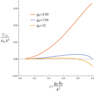
Figure 1: Numerical result for the dimensionless action density, as determined in Eq. (77), in terms of the dimensionless parameter $\zeta=\frac{g_{\text{R}}B_{\text{R}}}{k^{2}}\leqslant 1$, for various values of the renormalized coupling constant. Increasing the renormalized coupling $g_{\text{R}}$ results in an increasing but finite contribution of the quantum part of the one-loop effective action eventually dominating the classical one.

For small couplings, the classical contribution is dominating and quadratically increasing with the field strength. Modifications become visible only near the validity boundary $\zeta=\frac{g_{\text{R}}B_{\text{R}}}{k^{2}}=1$, where the unstable mode contributes strongest, cf. upper line for $g_{\text{R}}=3.5$, i.e. $\frac{\alpha_{\text{R}}}{4\pi}\simeq 0.08$. Extending the one-loop result ad hoc to even larger values of the coupling, the one-loop contribution becomes of similar order as the classical one near $g_{\text{R}}=7.94$, i.e. $\frac{\alpha_{\text{R}}}{4\pi}\simeq 0.4$, cf. middle line in Fig. 1. For even larger values of the coupling, the classical trivial ground state no longer remains the global minimum as is visible for the lowest line for $g_{\text{R}}=12$, i.e. $\frac{\alpha_{\text{R}}}{4\pi}\simeq 0.9$. The low-lying modes in the gluonic spectrum drive the system towards a state of nonvanishing field expectation value which may be taken as an indication for gluon condensation in the present setting.

Note that this follows from extrapolating the one-loop contribution to large coupling within the full validity domain of the one-loop effective action as our gauge-fixing allows to rigorously control the unstable-mode contribution. This is different from the conventional one-loop reasoning, where an analytic continuation of the gluon determinant is needed in order to arrive at a well-defined result. In the latter case, the final result is dominated by the one-loop counter-term $\sim\frac{11}{6}s^{2}B^{2}$ inside the propertime integral, and the one-loop action acquires the conventional $B^{2}\ln\frac{B^{2}}{k^{2}}$ form, which also exhibits a nontrivial minimum [108].

V.2 Selfdual background and gluon condensation

Addressing the generation of a gluon condensate requires a fully non-perturbative method. For instance, clear evidence is provided by an RG flow computation based on non-perturbative propagators [43], yielding satisfactory agreement with phenomenological estimates from spectral sum rules. In the present perturbative setting, it is nevertheless straightforwardly possible to find further indications for the onset of gluon condensation. For this, we use a Euclidean selfdual background field, e.g., with the choice

$$\mathsf{F}_{12}=\mathsf{F}_{34}=f=\text{const.},$$ (78)

for the abelian field strength. Using conventions analogous to the preceding subsection, the classical Yang-Mills action reduces to $\frac{1}{4}F_{\mu\nu}^{a}F_{\mu\nu}^{a}=f^{2}$, and the one-loop effective action can be expressed in terms of the variable

$$\bar{f}_{\ell}=\bar{g}f\nu_{\ell}.$$ (79)

The advantage of the selfdual background is that the corresponding spectrum of the gluonic transversal fluctuation operator $\mathfrak{D}_{\text{T}}$ does not have an unstable mode, but features a double zero mode [109]. Though this removes the instability encountered in the preceding subsection, the treatment of the zero mode still requires some care.

As a second ingredient, we choose the ghost mass term to vanish $\bar{m}_{\text{gh}}=0$ while we keep a finite gluon mass $\bar{m}>0$. In fact, this mimicks the so-called decoupling solution known from the nonperturbative study of gluon and ghost propagators [68, 69, 70, 71, 72, 73, 21, 74, 75, 76, 77, 78, 79, 80, 81]. A parametrization of these nonperturbative propagators in terms of massive gluons but massless ghosts works surprisingly successfully in phenomenological applications [8, 9, 10, 11, 12, 13, 14].

Analogously to the computation for the magnetic case in the preceding subsection, we can compute the corresponding determinants for the selfdual case using the explicit forms for the heat kernel (cf. [43]). Equivalently, the one-loop renormalization can be performed, yielding the same result for the running coupling. Here, we concentrate on the final form of the one-loop effective action in terms of the analogously renormalized field strength parameter $f_{\text{R}}$. Using the abbreviation $f_{\ell}=g_{\text{R}}f_{\text{R}}\nu_{\ell}$, the resulting renormalized one-loop action density reads

$$\frac{\Gamma_{\text{1L}}}{\Omega_{4}} =f_{\text{R}}^{2}$$ (80)

$$+\frac{1}{(4\pi)^{2}}\int_{0}^{\infty}\frac{\mathrm{d}s}{s^{3}}\sum_{\ell=1}^{N^{2}-1}$$

$$\times\Bigg{\{}\mathrm{e}^{-\bar{m}^{2}s}\Bigg{[}2+\frac{11(sf_{\ell})^{2}}{3}-\frac{2(s{f}_{\ell})^{2}}{\sinh^{2}\left(s{f}_{\ell}\right)}-{4(s{f}_{\ell})^{2}}\Bigg{]}$$

$$\qquad-\left(1-\frac{(f_{\ell}s)^{2}}{\sinh^{2}(f_{\ell}s)}\right)\Bigg{\}}.$$

Here, we have subtracted the counterterms completely within the gluon loop terms corresponding to the terms in square brackets; a naive separate subtraction of the gluon and ghost loops would artificially induce an IR divergence in the ghost term, and also render the wave function renormalization IR divergent. By contrast, the present subtraction prescription is a pure UV subtraction and renders the one-loop action UV and IR finite.

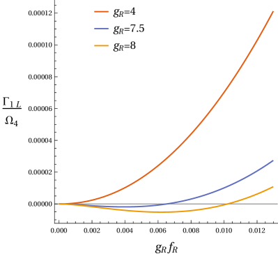
Figure 2: Action density for a selfdual background field, Eq. (80), in terms of the parameter $g_{\text{R}}B_{\text{R}}$. All quantities are plotted in units of the gluon mass which we choose as $\bar{m}^{2}=1$ here. An increase of the renormalized coupling beyond a critical coupling $g_{\text{cr}}\simeq 5$ results in the appearance of a nontrivial minimum which can be taken as an indication for a gluon condensate.

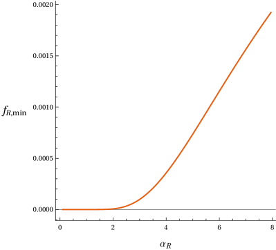
Figure 3: Gluon condensate $f_{\text{R,min}}$, in units of the gluon mass, corresponding to the nontrivial minimum of the action density as a function of the renormalized coupling $\alpha_{\text{R}}=\frac{g_{\text{R}}^{2}}{4\pi}$. Our result shows a continuous increase of the condensate beyond a critical coupling $\alpha_{\text{R}}>\alpha_{\text{cr}}\simeq 2$. The transition to a condensate phase is continuous.

The last term of the decomposition of the gluon loop in square brackets $\sim 4(sf_{\ell})^{2}$ corresponds to the zero-mode contribution. The latter introduces a subtlety: as is well known, there exists a nontrivial IR-UV interplay in the presence of zero modes [110]. Though the zero mode is clearly an IR feature of the spectrum, it can affect the strong-field limit of effective actions which are generically dominated by the UV properties of the theory. In the present case, the zero mode indeed spoils the large-field asymptotics, in the sense that this last term in square brackets leads to a large-field asymptotics $\sim-f^{2}\ln f^{2}/\bar{m}^{4}$ unbounded from below.

Since the zero mode does not contribute to the small-field behavior (it is subtracted by the counterterm), this artifact can be cured easily: we may multiply the zero-mode contribution with an IR-regularizing function that suppresses its large-field asymptotics, for instance, by the replacement $-4(sf_{\ell})^{2}\to-4(sf_{\ell})^{2}\exp(-s^{2}/L^{4})$. Here, $L\gg 1/\bar{m},\;1/\sqrt{f}$ can be thought of as a generic IR length scale over which the homogeneous selfduality assumption persists.

For the following study, the details of this IR regularization are not relevant. It suffices to know that a suitable cure of this artifact exists. Here, we concentrate on the properties of the effective action in the small-field region which is neither affected by the zero mode nor by the details of its regularization.

In Fig. 2, we depict the resulting one-loop effective action density for the case of SU(2) as a function of the selfdual field strength in units of the gluon mass parameter for increasing values of the coupling. We observe that the corresponding action density is dominated by the classical part for small renormalized couplings, cf. the line for $g_{\text{R}}=4$, i.e. $\alpha_{\text{R}}=\frac{g_{\text{R}}^{2}}{4\pi}\simeq 1.3$ which persists up to the critical coupling $g_{\text{cr}}\simeq 5$ (or $\alpha_{\text{cr}}\simeq 2$). Further increase of the renormalized coupling results in the development of a nontrivial vacuum expectation value, cf. lines for $g_{\text{R}}=7.5$ ($\alpha_{\text{R}}\simeq 4.5$) and $g_{\text{R}}=8$ ($\alpha_{\text{R}}\simeq 5.1$). The transition to the condensate phase at the critical coupling $\alpha_{\text{cr}}\simeq 2$ is continuous and the subsequent increase proceeds almost linearly with $\alpha_{\text{R}}$, see Fig. 3.

On the one hand, our approach appears capable of qualitatively addressing the question of gluon condensation using some nonperturbative input based on the decoupling solution for fully dressed propagators. On the other hand, our quantitative result for the value of the condensate depends on the choice for the gluon mass parameter $\bar{m}$ and further input for the IR behavior of the coupling. Choosing as an example $\bar{m}\simeq 1$GeV as a typical hadronic scale and the coupling in the range $\alpha_{\text{R}}\simeq 2\dots 8$ does, however, not lead to a value of the condensate that would match with phenomenological estimates [111]; the latter would correspond to $f_{\text{min}}\bar{m}^{2}\simeq 0.21\text{GeV}^{2}$ in our conventions. This poor quantitative accuracy is most likely due to the one-loop approximation adopted here.

VI Schwinger functional source term for covariantly constant backgrounds

To one-loop order, our nonlinear gauge fixing induces a structural difference to conventional formulations in the form of the 1PR contribution to the Schwinger functional, cf. Eq. (54). As the Schwinger functional generates all connected diagrams, contributing to $S$-matrix elements, this additional term is of general interest and is explored from different perspectives in this and the following sections. We confine ourselves to vanishing external sources $j=0$, see Eq. (47), such that Eq. (54) acquires the form

$$W_{\text{source}}[A,v]=\frac{1}{2}\mathcal{K}_{\mu}^{a}[A,v]\left({M^{-1}}\right)^{ab}_{\mu\nu}[A]\,\mathcal{K}_{\nu}^{b}[A,v],$$ (81)

where $\mathcal{K}$ has been defined in (55). A priori, $W_{\text{source}}$ depends independently on the background field $A$ as well as on the external $v$ field, even though these two fields are connected by a constraint, cf. Eq. (44). Whereas the background field has a natural physical interpretation, the $v$ field is part of the gauge fixing, hence, we expect that it does not contribute to observables.

At this point, we still have the freedom to choose a condition for the form of the background $A$ and external field $v$. In the present section, we focus on covariantly constant fields, satisfying Eq. (59). Provided the classical equations of motion are fulfilled, this directly implies that the current $J[A,v]$ carrying the $v$ field dependence, cf. Eq. (42), also has to vanish according to Eq. (41). The immediate conclusion is that the source term Eq. (81) vanishes identically (assuming the absence of relevant zero modes of $M$). This proves that – under these assumptions – the one-loop $S$-matrix elements are independent of the $v$ field of the gauge-fixing sector as expected.

However, it is instructive to relax these assumptions and keep the discussion slightly more general. From a physical perspective, the potential presence of unstable modes for covariantly constant fields, such as the pseudoabelian magnetic case used above, suggests to consider the covariantly-constant-field assumption as a local approximation to fields varying sufficiently slowly in space and time. We still assume vacuum conditions, i.e., the absence of external currents $j=0$, such that an on-shell stable background field configuration should be covariantly constant. However we no longer assume that the classical equations of motion Eq. (41) are fulfilled. While we now take $J[A,v]$ as potentially non-vanishing, consistency of the equation of motion requires $J$ to be covariantly conserved, $D_{\mu}J_{\mu}=0$, which we keep as an assumption also when $A$ is off-shell.

In addition, in this section we consider a more general form of the souce which is only assumed to be covariantly longitudinal,

$$J_{\mu}^{a}[A,v]=D_{\mu}^{ab}[A]\chi^{b},$$ (82)

where $\chi^{a}$ is an arbitrary auxiliary quantity. The special form of the source in Eq. (42) which is specific for a Fourier-noise implementation of the background-covariant gauge fixing can be recovered by appropriately choosing $\chi$.

For these choices, the source contribution Eq. (54) becomes

$$W_{\text{source}}[A,v]= \ \frac{1}{2}J_{\mu}^{a}[A,v]\left({M^{-1}}\right)^{ab}_{\mu\nu}[A]J_{\nu}^{b}[A,v].$$ (83)

For the concrete analysis, let us consider the gluonic mass parameter $\bar{m}$ to be sufficiently large. Also, we keep the gauge-fixing parameter $\xi$ general. In view of Eq. (81) we need the inverse gluonic fluctuation operator. For this, let us rewrite Eq. (53) as

$$M_{\mu\nu}^{ab}[A]=\bar{m}^{2}\delta_{\mu\nu}^{ab}+\mathcal{Q}_{\mu\nu}^{ab}[A],$$ (84)

where

$$\mathcal{Q}_{\mu\nu}^{ab}[A]=2\bar{g}f^{abc}F_{\mu\nu}^{c}-\left({D^{2}}\right)^{ab}\delta_{\mu\nu}+\left({1-\frac{1}{\xi}}\right)D_{\mu}^{ac}D_{\nu}^{cb}.$$ (85)

The gluonic fluctuation operator and its inverse, schematically are given by

$$M =\bar{m}^{2}\left[{\mathbb{1}+\bar{m}^{-2}\mathcal{Q}}\right],\quad M^{-1}=\bar{m}^{-2}\left[{\frac{1}{1+\bar{m}^{-2}\mathcal{Q}}}\right].$$ (86)

As we assume the gluonic mass to be sufficiently large, we expand the gluon propagator in powers of the operator $\mathcal{Q}$,

$$\left({M^{-1}}\right)^{ab}_{\mu\nu}=-\sum_{n=0}^{\infty}{\left[{\left({\frac{i}{\bar{m}}}\right)^{2n+2}\left({\mathcal{Q}^{n}}\right)_{\mu\nu}^{ab}}\right]},$$ (87)

where $\left({\mathcal{Q}^{n}}\right)_{\mu\nu}^{ab}=\underbrace{\mathcal{Q}^{ac}_{\mu\rho}\mathcal{Q}^{cd}_{\rho\sigma}\cdots\mathcal{Q}_{\kappa\tau}^{er}\mathcal{Q}^{rb}_{\tau\nu}}_{\text{$n$ times}}$ was used. It is useful to decompose the operator $\mathcal{Q}_{\mu\nu}$ in terms of the longitudinal $\mathfrak{D}_{\text{L}}$ and transversal $\mathfrak{D}_{\text{T}}$ kinetic operators

$$\mathcal{Q}_{\mu\nu}^{ab}[A] =\left({\mathfrak{D}_{\text{\text{T}}}}\right)_{\mu\nu}^{ab}-\left({1-\frac{1}{\xi}}\right)\left({\mathfrak{D}_{\text{\text{L}}}}\right)_{\mu\nu}^{ab},$$ (88)

where

$$\left({\mathfrak{D}_{\text{\text{T}}}}\right)_{\mu\nu}^{ab}= -\delta_{\mu\nu}\left({D^{2}}\right)^{ab}+2i\bar{g}F_{\mu\nu}^{ab},$$ (89)

$$\left({\mathfrak{D}_{\text{L}}}\right)_{\mu\nu}^{ab}= -D_{\mu}^{ac}D_{\nu}^{cb}.$$ (90)

The latter are further discussed in [28, 29, 30]. Some useful properties of these kinetic operators for the present case are

$$\left[{\mathfrak{D}_{\text{T}},\mathfrak{D}_{\text{L}}}\right]_{\mu\nu}^{ab} =0,$$ (91)

$$\left({\mathfrak{D}_{\text{\text{L}}}}\right)_{\mu\nu}^{ab}J_{\nu}^{b} =0,\quad J_{\mu}^{a}\left({\mathfrak{D}_{\text{\text{L}}}}\right)_{\mu\nu}^{ab}=0.$$ (92)

Eq. (91) relies on the assumption of covariantly constant background field. Equations (92) are a direct consequence of the definition of the longitudinal kinetic operator given by Eq. (90) and of current conservation.

The source contribution to the Schwinger functional, Eq. (83), now takes the following form in the large-mass expansion

$$W_{\text{source}}[A,v] =-\frac{1}{2}J_{\mu}^{a}\sum_{n=1}^{\infty}{\left[{\left({\frac{i}{\bar{m}}}\right)^{2n+2}\left({\mathfrak{D}_{\text{T}}^{n}}\right)_{\mu\nu}^{ab}}\right]}J_{\nu}^{b}$$ (93)

which highlights that the longitudinal contributions of the gluon propagator and thus any gauge-parameter $\xi$ dependence drops out of the 1PR source term as a consequence of Eqs. (91) and (92). For the evaluation of Eq. (93), we need the following commutator valid for covariantly constant background fields

$$\left[{D^{2},D_{\mu}}\right]^{ab}=-2i\bar{g}F_{\alpha\mu}^{ac}D_{\alpha}^{cb}.$$ (94)

Then, using the fact that the current has a longitudinal form, cf. Eq. (82), we obtain from the definition of $\mathfrak{D}_{\text{T}}$ in Eq. (89),

$$\mathfrak{D}_{\text{T},\mu\nu}^{ab}J^{b}_{\nu} = -(D^{2})^{ab}D_{\mu}^{bc}\chi^{c}+2i\bar{g}F^{ab}_{\mu\nu}J^{b}_{\nu}$$ (95)

$$= D_{\mu}^{ab}D_{\alpha}^{bc}J_{\alpha}^{c}-2i\bar{g}F^{ab}_{\mu\nu}J^{b}_{\nu}+2i\bar{g}F^{ab}_{\mu\nu}J^{b}_{\nu}$$

$$= 0.$$

Here, the first term on the right-hand side vanishes due to current conservation and the other two cancel. Hence we conclude that the 1PR source contribution to the Schwinger functional ,

$$\left.J_{\mu}^{a}\left({M^{-1}}\right)^{ab}_{\mu\nu}J_{\nu}^{b}\ \right|_{DF=0,DJ=0}=0,$$ (96)

vanishes for covariantly constant backgrounds and for a conserved and longitudinal current $J[A,v]$ to all orders in the large-mass expansion. Note that the equations of motion for the background field are consistent with these assumptions, even entail them, but need not be satisfied in itself for the conclusion to hold. Equation (96) also holds true in the case where the current is given by Eq. (42). In fact in this case the current is covariantly longitudinal, and in addition current conservation can be used to show that $J=0$.

Alternatively, we could have imposed the consistency condition for the $v$ field, Eq. (44), that arises from current conservation. In fact, if this consistency condition is satisfied, then the auxiliary quantity $\chi^{b}$ introduced above vanishes identically and so does the current $J[A,v]$. In this case, Eq. (96) is satisfied as well independently of the background field, assuming the absence of relevant zero modes of the gluon propagator.

In either case, this leads to an expression for the one-loop Schwinger functional

$$-W_{\text{1L}}[A]\bigg{|}_{DF=0,D\cdot J=0} = S_{\text{v}}[A]-\ln\Delta_{\text{FP}}[A]$$ (97)

$$+\frac{1}{2}\ln\det M[A],$$

being independent of any $v$ contribution and thus of the nonlinear gauge-fixing sector except for the BRST invariant mass terms. As a consequence, one-loop $S$-matrix elements also remain independent of the $v$ field as expected.

VII Schwinger Functional with a disorder $v$ field

The choice of a Fourier weight in the implementation of the gauge-fixing procedure, see Section II, leads to a $v$-dependent generating functional, Eq. (18). The linear part of the gauge fixing condition, Eq. (26), introduces a further source of $v$ dependence, which subsequently leads to 1PR terms in the Schwinger functional and also affects the Faddeev-Popov determinant. As shown before, one-loop results become independent again once consistency and/or on-shell conditions are used. However, from a practical viewpoint, it can be useful to have a computational formalism where no implementation of consistency/on-shell conditions at certain stages is required.

It is useful to think of the $v$ field as a gauge-parameter field. The most common implementation of the gauge-fixing condition is through a Gaussian averaging over the noise. The latter would correspond to a Gaussian average over the $v$ field. This averaging can either be implemented as an annealed or quenched disorder. While the former prescription coincides with a standard Gaussian Nakanishi-Lautrup sector, the latter is less trivial and we therefore find it interesting to analyze. In detail, we focus on the following quenched average over the external Nakanishi-Lautrup field of the Schwinger functional

$$W_{\text{1L}}[A] =\mathcal{N}\int{\mathcal{D}v\;e^{-S_{\mathrm{NL}}[v]}\;W_{\text{1L}}[A,v]},$$ (98)

$$S_{\mathrm{NL}}[v] =\int{\!\mathrm{d}^{d}x\,\frac{v^{2}}{2\alpha}},$$ (99)

where $\mathcal{N}$ is a normalization constant fixed by normalizing the free quenched average to unity.

Then, the terms that originate from the $v$ dependence and their effects can be studied. As only the last contribution in Eq. (50) is changed by this averaging, it is useful to denote

$$W_{\text{source}}[A]=-\frac{\mathcal{N}}{2}\int\mathcal{D}v\;e^{-S_{\mathrm{NL}}[v]}\;W_{\text{source}}[A,v].$$ (100)

Note that a generic $v$ field as a representative of all configurations to be integrated over will generally not satisfy the consistency condition (44) for a given background field. Whether or not such violations affect final results or may average out thus needs to be investigated. In the following, we will do so on the one-loop level where the $v$ field occurs only in the 1PR source term of the Schwinger functional, whereas the effective action remains unaffected.

With regard to the structure of the current $J[A,v]$ that carries the $v$ dependence inside the source term $W_{\text{source}}[A,v]$, cf. Eq. (44), we split the current into the derivative term and the term containing the ghost mass, and write the source term as,

$$W_{\text{source}}[A]=-\left({\frac{1}{2}}\right)\int\mathcal{D}v\;\mathrm{e}^{-\int{\frac{v^{2}}{2\alpha}}} \left[{\left({D_{\mu}v}\right)^{a}\left({M^{-1}}\right)_{\mu\nu}^{ab}\left({D_{\nu}v}\right)^{b}}\right.\qquad\qquad\qquad\qquad\qquad\qquad\;\;\;\;\;\;\text{(i)}$$ (101)

$$\quad-\bar{m}_{\text{gh}}^{2}\left({D_{\mu}v}\right)^{a}\left({M^{-1}}\right)_{\mu\nu}^{ab}\left({D_{\nu}\left({\frac{1}{D^{2}}}\right)v}\right)^{b}\qquad\qquad\qquad\;\text{(ii)}$$

$$\quad-\bar{m}_{\text{gh}}^{2}\left({D_{\mu}\left({\frac{1}{D^{2}}}\right)v}\right)^{a}\left({M^{-1}}\right)_{\mu\nu}^{ab}\left({D_{\mu}v}\right)^{b}\qquad\qquad\;\;\;\;\;\;\;\;\text{(iii)}$$

$$\quad\left.{+\bar{m}_{\text{gh}}^{4}\left({D_{\mu}\left({\frac{1}{D^{2}}}\right)v}\right)^{a}\left({M^{-1}}\right)_{\mu\nu}^{ab}\left({D_{\nu}\left({\frac{1}{D^{2}}}\right)v}\right)^{b}}\right].\quad\;\;\;\text{(iv)}$$

Performing the Gaussian functional integral, the four terms can be written as traces in coordinate, color and Lorentz space,

(i) $$=\left({\frac{\alpha}{2}}\right)\operatorname{tr}_{\text{xcL}}{\left[{D_{\mu}M^{-1}_{\mu\nu}D_{\nu}}\right]}$$ (102a)

(ii, iii) $$=-\left({\frac{\alpha\bar{m}_{\text{gh}}^{2}}{2}}\right)\operatorname{tr}_{\text{xcL}}{\left[{\frac{1}{D^{2}}D_{\mu}M^{-1}_{\mu\nu}D_{\nu}}\right]}$$ (102b)

(iv) $$=\left({\frac{\alpha\bar{m}_{\text{gh}}^{4}}{2}}\right)\operatorname{tr}_{\text{xcL}}{\left[{\frac{1}{D^{2}}\frac{1}{D^{2}}D_{\mu}M^{-1}_{\mu\nu}D_{\nu}}\right]},$$ (102c)

where the cyclicity of the trace has been taken into account. As the gluon propagator $M^{-1}$ is sandwiched between covariant derivatives, the transversal parts drop out and we obtain

(i) $$=\left({\frac{\alpha}{2}}\right)\operatorname{tr}_{\text{xcL}}{\left[{\frac{1}{\bar{m}^{2}-\left({\frac{1}{\xi}}\right)D^{2}}D^{2}}\right]}$$ (103a)

(ii, iii) $$=-\left({\frac{\alpha\bar{m}_{\text{gh}}^{2}}{2}}\right)\operatorname{tr}_{\text{xcL}}{\left[{\frac{1}{D^{2}}\frac{1}{\bar{m}^{2}-\left({\frac{1}{\xi}}\right)D^{2}}D^{2}}\right]}$$ (103b)

(iv) $$=\left({\frac{\alpha\bar{m}_{\text{gh}}^{4}}{2}}\right)\operatorname{tr}_{\text{xcL}}{\left[{\frac{1}{D^{2}}\frac{1}{D^{2}}\frac{1}{\bar{m}^{2}-\left({\frac{1}{\xi}}\right)D^{2}}D^{2}}\right]}.$$ (103c)

It is interesting to note that all terms are proportional to the width parameter $\alpha$ of the quenched disorder field; this implies that all terms vanish in the limit $\alpha\to 0$. In this limit, the amplitude of $v$ as a disorder field vanishes, such that the consistency condition Eq. (44) is evidently satisfied as also is current conservation, imposed explicitly in the preceding section. Still at this point, one may wonder whether the occurrence of inverse Laplacians may lead to ill-defined expressions.

In order to obtain more explicit results, let us evaluate the traces for a covariantly constant, pseudoabelian magnetic field, as also used before, see Section V. It is already interesting to note for this case that none of the above traces are affected by the unstable Nielsen-Olesen mode which has dropped out as a consequence of the implicit longitudinal projection. For convenience, we introduce auxiliary functions that capture the dependence of the operators to be traced on the Laplacian. E.g., for the first term (i), we introduce

$$h_{\text{(i)}}(x)=-\frac{\xi x}{x+\xi\bar{m}^{2}},$$ (104)

such that the trace in Eq. (103a) can be written as

$$\left.{\operatorname{tr}_{\text{xcL}}{\left[{h_{\text{(i)}}(x)}\right]}}\right|_{x=-D^{2}}=-\left.{\operatorname{tr}_{\text{xcL}}{\left[{\frac{\xi x}{x+\xi\bar{m}^{2}}}\right]}}\right|_{x=-D^{2}}.$$ (105)

The trace can be evaluated with heat-kernel techniques using the Laplace transform of the auxiliary function $h_{\text{(i)}}$ which leads us to the propertime representation. As before, we normalize the results by a constant subtraction such that the terms vanish at zero background field. For the trace, we find

$$\operatorname{tr}_{\text{xcL}}{\left[{h_{\text{(i)}}\left({-D^{2}}\right)-h_{\text{(i)}}\left({-\partial^{2}}\right)}\right]}=-{\frac{\Omega_{4}}{\left({4\pi}\right)^{2}}}\sum_{\ell=1}^{N^{2}-1}$$ (106)

$$\times{\int_{0}^{\infty}{\frac{ds}{s^{2}}}}\left[{\left({\xi\bar{m}}\right)^{2}\mathrm{e}^{-\xi\bar{m}^{2}s}-2\xi\delta(s)}\right]\left[{\frac{sB_{\ell}}{\sinh{sB_{\ell}}}-1}\right],$$

where the $\delta$ function at the integral boundary is understood to contribute with half of its weight. We observe that the result is finite, the integral converges at both boundaries; moreover, it vanishes in the Landau gauge limit $\xi\to 0$. It is furthermore instructive to study the small-field limit at order $B^{2}$ which, on the level of the effective action, would correspond to the classical terms contributing to the renormalization of the charge and the field strength. It is straightforward to check that these possible lowest order terms of Eq. (106) vanish,

$$\frac{1}{\Omega_{4}}\text{(i)}_{\text{vs}}=0+\mathcal{O}(B^{4}/\bar{m}^{8}),$$ (107)

where the subscript ’vs’ denotes vacuum subtraction.

The same computational steps can be applied to the terms (ii) and (iii), cf. Eq. (103b), using the auxiliary function

$$h_{\text{(ii)}}(x)=\frac{\xi}{x+\xi\bar{m}^{2}}.$$ (108)

The corresponding vacuum subtracted trace yields

$$\operatorname{tr}_{\text{xcL}}{\left[{h_{\text{(ii)}}\left({-D^{2}}\right)-h_{\text{(ii)}}\left({-\partial^{2}}\right)}\right]}$$ (109)

$$=\Omega_{4}{\frac{\xi}{\left({4\pi}\right)^{2}}}\sum_{\ell=1}^{N^{2}-1}{\int_{0}^{\infty}{\frac{ds}{s^{2}}\mathrm{e}^{-\xi\bar{m}^{2}s}\left[{\frac{sB_{\ell}}{\sinh{sB_{\ell}}}-1}\right]}}.$$

Again, we observe that the integral expression is finite and vanishes in the Landau-gauge limit $\xi\to 0$. For this term, we obtain a contribution to quadratic order,

$$\frac{1}{\Omega_{4}}\text{(ii, iii)}_{\text{vs}}=$$ (110)

$$\quad\left({\frac{1}{4\pi}}\right)^{2}\left({\frac{\bar{m}_{\text{gh}}}{\bar{m}}}\right)^{2}\left({\frac{\alpha}{12}}\right)N_{\text{c}}\,(\bar{g}B)^{2}+\mathcal{O}(B^{4}/\bar{m}^{8}).$$

Note that the absence of the gauge parameter is a result of the expansion which is valid only for $\bar{g}B/(\xi\bar{m}^{2})\ll 1$ and does not include the Landau-gauge limit.

For the fourth functional trace, Eq. (103c), we introduce the auxiliary function

$$h_{\text{(iv)}}(x)=-\frac{\xi}{x\left({x+\xi\bar{m}^{2}}\right)}$$ (111)

which leads to the explicit form of the vacuum subtracted functional trace

$$\operatorname{tr}_{\text{xcL}}{\left[{h_{\text{(iv)}}\left({-D^{2}}\right)-h_{\text{(iv)}}\left({-\partial^{2}}\right)}\right]}=-{\frac{\Omega_{4}}{\left({4\pi\bar{m}}\right)^{2}}}\sum_{\ell=1}^{N^{2}-1}{|B_{\ell}|}$$ (112)

$$\times{\int_{0}^{\infty}\frac{dx}{x^{2}}\left[{1-\mathrm{e}^{-\frac{\xi\bar{m}^{2}}{|B_{\ell}|}x}}\right]\left[{\frac{x}{\sinh{x}}-1}\right]},$$

where we substituted $x=s|B_{\ell}|$. Again, the integral is finite and vanishes in the Landau-gauge limit $\xi\to 0$. As an interesting feature, we observe that the integral in Eq. (112) approaches a finite constant in the small-field limit. Up to quadratic order, the expansion yields

$$\frac{1}{\Omega_{4}}\text{(iv)}_{\text{vs}}=-\left({\frac{1}{4\pi}}\right)^{2}\left({\frac{\bar{m}_{\text{gh}}}{\bar{m}}}\right)^{4}\left({\frac{\alpha}{2}}\right)$$ (113)

$$\times\left[\bar{m}^{2}\ln\left(\frac{1}{2}\right)\sum_{\ell=1}^{N^{2}-1}|B_{\ell}|+\frac{1}{6\xi}N_{\text{c}}(\bar{g}B)^{2}\right]+\mathcal{O}(B^{4}/\bar{m}^{8}).$$

The occurrence of the term linear in $B_{\ell}\sim\bar{g}B$ is noteworthy as this term would be invisible in a small-field expansion which is an expansion in $(\bar{g}B)^{2}$. As before, the dependence of the quadratic term on $1/\xi$ is a result of the expansion which becomes invalid in the Landau-gauge limit. The full expression vanishes in the Landau gauge $\xi=0$.

Collecting all results which were derived for the functional traces in the weak-field expansion, Eq. (107), Eq. (110) & Eq. (113) and inserting into the source contribution to the Schwinger functional, Eq. (101), then

$$W_{\text{source}}[A]$$ (114)

$$=\frac{\Omega_{4}}{\left({4\pi}\right)^{2}}\left({\frac{\bar{m}_{\text{gh}}}{\bar{m}}}\right)^{2}\left({\frac{\alpha}{2}}\right)\left[{-\bar{m}^{2}\ln{\left({\frac{1}{2}}\right)\sum_{l=1}^{N^{2}-1}\left|{B_{\ell}}\right|}}\right.$$

$$\qquad\qquad\qquad\qquad\qquad\quad+\left.{\frac{\bar{g}^{2}N_{c}}{6}\left({1-\frac{\bar{m}_{\text{gh}}^{2}}{\xi\bar{m}^{2}}}\right)B^{2}}\right].$$

We observe that only the linear $B$-field term remains for the special choice of $\bar{m}_{\text{gh}}^{2}=\xi\bar{m}^{2}$.

The one-loop Schwinger functional takes the form

$$-W_{\text{1L}}[A]= S_{\text{v}}[A]-\ln\Delta_{\text{FP}}[A]+\frac{1}{2}\ln\det M[A]$$ (115)

$$-W_{\text{source}}[A].$$

In summary, we find that a treatment of the $v$ field as a quenched disorder field yields finite contributions to the 1PR source term in the Schwinger functional; of course, by averaging over $v$ this term becomes 1PI, as the quenched average corresponds to connecting the $v$-field legs. The implicit violation of the consistency condition (44) does not immediately cancel in the disorder average. Nevertheless we observe that these contributions can be controlled in various ways: first and importantly, they stay finite despite the nonlocal structure introduced by inverse Laplacians, second they vanish in the limit of both $\alpha\to 0$ (vanishing disorder amplitude) as well as $\xi\to 0$ (Landau gauge). All terms remain subdominant to the one-loop action or even vanish in the large-field limit and can also be controlled in a small-field expansion, even though the appearance of a finite term linear in $|B|$ signals the presence of non-analyticities at vanishing field strength.

For the case of a constant magnetic field, also the Nielsen-Olesen unstable mode does not play any role. Provided that these properties translate to higher-loops or even nonperturbative computations, the treatment of the $v$ field as a disorder field can be a useful computational strategy to deal with this gauge degree of freedom.

VIII $v$-Field Contributions to the Connected Background 2-point Function

Whereas the one-loop Schwinger functional is independent of the $v$ field on-shell, off-shell contributions to the connected background 2-point function are expected to appear from the 1PR source term, Eq. (54). In the following, we determine these contributions explicitly in the limit of vanishing background $A\rightarrow 0$ and external source $j\to 0$, see Eq. (47) for the definition of $j$. I.e., we study

$$W^{(2)}_{v}=\frac{\delta^{2}W_{\text{source}}[j,A,v]}{\delta A\delta A}\Big{|}_{A,j\to 0},$$ (116)

where $W_{\text{source}}[j=0,A,v]=\frac{1}{2}\mathcal{K}M^{-1}\mathcal{K}$, cf. Eq. (81). Since $\mathcal{K}=DF+J$, the limit of vanishing background field yields for this quantity using Eq. (42),

$$\mathcal{K}_{\mu}^{a}\big{|}_{A\to 0}=J_{\mu}^{a}\big{|}_{A\to 0}=\partial_{\mu}\left({1+\frac{\bar{m}_{\text{gh}}^{2}}{-\partial^{2}}}\right)v^{a},$$ (117)

which corresponds to the external current discussed in Ref. [15]. Now, current conservation implies the consistency condition (44), requiring the $v$ field to satisfy the massive Klein-Gordon equation in absence of a background

$$0=\left.{D_{\mu}^{ab}J_{\mu}^{b}}\right|_{A\rightarrow 0}=\left({\partial^{2}-\bar{m}_{\text{gh}}^{2}}\right)v^{a}.$$ (118)

Combining Eqs. (117) and (118) tells us that the source term vanishes in absence of a background

$$\mathcal{K}_{\mu}^{a}\big{|}_{A\to 0}=J_{\mu}^{a}\big{|}_{A\to 0}=0.$$ (119)

Correspondingly, the functional derivatives of Eq. (116) acting on the 1PR source term, Eq. (81), only yield finite contributions in the $A\to 0$ limit as long as they act on the $\mathcal{K}$ factors. A crucial building block is given by $\delta J/\delta A$ which is derived in the Appendix in Eq. (150). Furthermore, we need the gluon propagator $M^{-1}$ for vanishing fields which, in our gauge, reads schematically

$$M^{-1}\big{|}_{A\rightarrow 0}=\left({\frac{1}{\bar{m}^{2}-\partial^{2}}}\right)\Pi_{\text{T}}+\left({\frac{1}{\bar{m}^{2}-\frac{\partial^{2}}{\xi}}}\right)\Pi_{\text{L}},$$ (120)

where we have used the longitudinal and transversal projectors

$$\left({\Pi_{\text{L}}}\right)_{\mu\nu}^{ab}=\left({\frac{\partial_{\mu}\partial_{\nu}}{\partial^{2}}}\right)\delta^{ab},\quad\left({\Pi_{\text{T}}}\right)_{\mu\nu}^{ab}=\delta_{\mu\nu}\delta^{ab}-\left({\Pi_{\text{L}}}\right)_{\mu\nu}^{ab}.$$ (121)

The building blocks for the 2-point function contributions from the source term using the preceding results in momentum space together with Eq. (150) thus read,

$$\frac{1}{2} \left.{\frac{\delta^{2}\left[{J_{\mu}^{a}\left({M^{-1}}\right)^{ab}_{\mu\nu}J_{\nu}^{b}}\right]}{\delta A_{\alpha}^{c}(p_{1})\delta A_{\beta}^{d}(p_{2})}}\right|_{A\rightarrow 0}$$ (122)

$$=\bar{g}^{2}f^{abc}f^{aed}\int_{q}\frac{\left({2q+p_{1}}\right)_{\alpha}}{\bar{m}^{2}+\frac{q^{2}}{\xi}}\frac{\left({2q-p_{2}}\right)_{\beta}}{q^{2}}v_{-q-p_{1}}^{e}v_{q-p_{2}}^{b},$$

$$\frac{1}{2} \left.{\frac{\delta^{2}\left[{\left({DF}\right)_{\mu}^{a}\left({M^{-1}}\right)^{ab}_{\mu\nu}\left({DF}\right)_{\nu}^{b}}\right]}{\delta A_{\alpha}^{c}(p_{1})\delta A_{\beta}^{d}(p_{2})}}\right|_{A\rightarrow 0}$$ (123)

$$=\delta^{cd}\frac{p_{1}^{2}}{\bar{m}^{2}+p_{{1}}^{2}}\left({p_{1}^{2}\delta_{\alpha\beta}-p_{1\alpha}p_{1\beta}}\right)\delta_{p_{1},-p_{2}},$$

$$\!\!\!\!\!\left.{\frac{\delta^{2}\left[{J_{\mu}^{a}\left({M^{-1}}\right)^{ab}_{\mu\nu}\left({DF}\right)_{\nu}^{b}}\right]}{\delta A_{\alpha}^{c}(p_{1})\delta A_{\beta}^{d}(p_{2})}}\right|_{A\rightarrow 0}=0.$$ (124)

Whereas the $v$-independent contribution in Eq. (123) is diagonal in momentum space, the $v$-dependent one from Eq. (122) is not. These nondiagonal parts parametrize the momentum-influx into the 2-point function provided by a possibly space-time dependent $v$ field. The sum of Eqs. (122) and (123) represents the general result for the contributions from the 1PR source term of the Schwinger functional to the 2-point correlator at this order for $v$ fields that satisfy the consistency condition, i.e. solve the massive Klein-Gordon equation.

Although we assumed current conservation, it is interesting to average Eq. (122) and Eq. (123) over $v$ with a Gaussian distribution, constrained by the requirement that the Klein-Gordon equation, Eq. (118), holds. The latter constraint can be implemented by means of a Lagrange multiplier field $\lambda^{a}$. Hence we integrate both terms by means of the formulas

$$\braket{1}=\mathcal{N}\int\!\!\mathcal{D}\lambda^{a}\mathcal{D}v^{a}\mathrm{e}^{\mathrm{i}\lambda^{a}(-\partial^{2}+\bar{m}_{\mathrm{gh}}^{2})v^{a}-\frac{v^{a}v^{a}}{2\alpha}}\!=\!1,$$ (125)

$$\braket{v^{a}_{p}v^{b}_{q}}=\mathcal{N}\int\!\!\mathcal{D}\lambda^{a}\mathcal{D}v^{a}\mathrm{e}^{\mathrm{i}\lambda^{a}(-\partial^{2}+\bar{m}_{\mathrm{gh}}^{2})v^{a}-\frac{v^{a}v^{a}}{2\alpha}}v^{a}_{p}v^{b}_{q}=0.$$ (126)

where the normalization constant $\mathcal{N}$ is fixed by the requirement of Eq. (125).

After averaging over the $v$ field, Eq. (122) will not contribute to the $v$-independent 2-point function, as a result of Eq. (126). The remaining term arising from Eq. (123) then yields the source contribution to the averaged 2-point function

$$\braket{W^{(2)}_{v}(p_{1},p_{2})}^{cd}_{\alpha\beta}=\frac{\delta^{cd}p_{1}^{4}}{\bar{m}^{2}+p_{{1}}^{2}}\left(\delta_{\alpha\beta}-\frac{p_{1\alpha}p_{1\beta}}{p_{1}^{2}}\right)\delta_{p_{1},-p_{2}}$$ (127)

The inverse $(W^{(2)}_{v})^{-1}$ of this function is a propagator type quantity. For this, we observe that $(W^{(2)}_{v})^{-1}\sim 1/p_{1}^{{2}}$ decays as usual in momentum space for large momenta implying that $S$-matrix contributions in the perturbative domain are not enhanced. At the same time, the $\sim 1/p_{1}^{4}$ behavior at small momenta is reminiscent to infrared slavery going hand in hand with the mass gap of the background field excitations.

Let us go back to the non-averaged case where, for concreteness, we consider the special case of a homogeneous $v$ field

$$v_{q}^{a}=v^{a}\sqrt{\left({2\pi}\right)^{d}}\delta(q).$$ (128)

In this case, the consistency condition (118) can be satisfied only for a vanishing ghost mass $\bar{m}_{\text{gh}}=0$ which we assume here in addition. The final result for $W^{(2)}_{v}$ then is diagonal in momentum space and reads

$$W^{(2)}_{v} (p|v)^{cd}_{\alpha\beta}=\bar{g}^{2}f^{abc}f^{aed}v^{b}v^{e}\delta_{p_{1},-p_{2}}$$ (129)

$$\times\left\{{\left[{\delta_{\alpha\beta}-{\frac{p_{1\alpha}p_{1\beta}}{p_{1}^{2}}}}\right]{\frac{1}{\bar{m}^{2}+p_{1}^{2}}}}{+{\frac{p_{1\alpha}p_{1\beta}}{p_{1}^{2}}}{\frac{1}{\bar{m}^{2}+\frac{p_{1}^{2}}{\xi}}}}\right\}$$

$$+\ \delta^{cd}\frac{p_{1}^{4}}{\bar{m}^{2}+p_{1}^{2}}\left({\delta_{\alpha\beta}-\frac{p_{1\alpha}p_{1\beta}}{p_{1}^{2}}}\right)\delta_{p_{1},-p_{2}}.$$

For general gauge parameter, we observe transversal and longitudinal contributions; pure transversality occurs in the Landau gauge where longitudinal parts decouple completely. The $v$-dependent parts affect only modes which are orthogonal to the $v$ field in color space.

Equation (129) can also be averaged over all possible directions of the constant vector $v^{a}$, with a Gaussian weight. For this kind of average, which is more constrained than the one considered in Eqs. (125) and (126), also the first term on the r.h.s. of Eq. (129) would bring a nonvanishing contribution. Notice however that the latter would remain finite and would not modify the structure of one-loop renormalization constants. By contrast, in Ref. [15], constant $v^{a}$ fields have been observed to yield nonvanishing contributions to the running of the wave function renormalization of the fluctuation field, in absence of a background, with or without averaging over $v^{a}$.

IX $v[A]$-Field Contributions to the Connected Background 2-point Function

The requirements of current conservation implied by the background equations of motion impose the consistency condition (44) on the $v$ field. So far, we have implemented this condition at various stages of our studies. In particular in the preceding section, we have made use of the consistency condition, once we have varied the 1PR source term of the Schwinger functional with respect to the background field. Alternatively, we may assume that the consistency condition is satisfied from the beginning, rendering the $v$ field a functional of the background, $v=v[A]$. Correnspondingly, the connected background 2-point function will receive additional contributions, as is analyzed in the following.

The difference to the result from the previous section arises from the derivative of the current,

$$\frac{\delta J[A,v[A]]}{\delta A}=\frac{\delta J[A,v]}{\delta A}\Big{|}_{v=v[A]}+N,$$ (130)

where the first term on the right-hand side first appeared in the preceding section and was computed in (150). Denoting

$$\mathrm{v}^{a} =v[A\to 0],\qquad\frac{\delta\mathrm{v}^{a}}{\delta A_{\alpha}^{c}}=\frac{\delta{v}^{a}}{\delta A_{\alpha}^{c}}\Bigg{|}_{A\to 0},$$ (131)

the additional term $N$ for $A\to 0$ reads

$$\left({N_{\mu\alpha}^{ac}}\right)_{xy}\Big{|}_{A\to 0} = \partial_{\mu}^{x}\left({\frac{\delta\mathrm{v}_{x}^{a}}{\delta A_{\alpha y}^{c}}}\right)$$

$$-\bar{m}_{\text{gh}}^{2}\int_{w}{\left({\frac{1}{\partial^{2}}}\right)_{xw}\;\partial_{\mu}^{w}\left({\frac{\delta\mathrm{v}_{w}^{a}}{\delta A_{\alpha y}^{c}}}\right)}.$$

This $N$ term gives rise to additional contributions to the connected background 2-point correlator not accounted for in the preceding section. The necessary functional derivative $\delta v/\delta A$ can be extracted from the consistency condition

$$(D^{2}-\bar{m}_{\text{gh}}^{2})v[A]=0.$$ (133)

Taking the functional derivative of this equation with respect to the background, yields in the limit $A\to 0$

$$\int_{z}{\left.{\frac{\delta\left({D^{2}}\right)^{ab}_{xz}}{\delta A_{\alpha y}^{c}}}\right|_{A\rightarrow 0}\mathrm{v}_{z}^{b}}=(\partial_{x}^{2}-\bar{m}_{\text{gh}}^{2})\left({\frac{\delta\mathrm{v}_{x}^{a}}{\delta A_{\alpha y}^{c}}}\right).$$ (134)

Multiplying both sides by the kernel of the Klein-Gordon operator allows us to solve for the desired functional derivative, which in momentum space reads

$$\left.{\frac{\delta v^{a}_{q}}{\delta A_{\alpha p}^{c}}}\right|_{A\rightarrow 0}=-i\bar{g}f^{abc}\left({\frac{1}{\bar{m}_{\text{gh}}^{2}+q^{2}}}\right)\left({2q-p}\right)_{\alpha}\mathrm{v}_{q-p}^{b}.$$ (135)

Upon insertion into Eq. (IX) and subsequently into Eq. (130), the essential building block for the 2-point function is the current derivative which now becomes

$$\left.{\frac{\delta J_{\mu q}^{a}}{\delta A_{\alpha p}^{c}}}\right|_{A\rightarrow 0}\!\!\!=-\bar{g}f^{abc}{\frac{q_{\mu}\left({2q-p}\right)_{\alpha}}{q^{2}}}\left[{1-\frac{p^{2}-2p\cdot q}{\bar{m}_{\text{gh}}^{2}+q^{2}}}\right]\mathrm{v}_{q-p}^{b}.$$ (136)

This equation replaces Eq. (150) as used in the preceding section. Correspondingly, using Eq. (136) in the analogue of Eqs. (122) and (123), we arrive at the following result for the background 2-point function arising from the 1PR source term

$$W^{(2)}_{v}(p_{1},p_{2}|v)^{cd}_{\alpha\beta} = \delta^{cd}\frac{p_{1}^{2}}{\bar{m}^{2}+p_{1}^{2}}\left({p_{1}^{2}\delta_{\alpha\beta}-p_{1\alpha}p_{1\beta}}\right)\delta_{p_{1},-p_{2}}+\bar{g}^{2}f^{abc}f^{aed}\int_{q}{\left({\frac{1}{\bar{m}^{2}+\frac{q^{2}}{\xi}}}\right)\left({\frac{1}{q^{2}}}\right)\left({2q+p_{1}}\right)_{\alpha}}\left({2q-p_{2}}\right)_{\beta}$$

$$\!\times\left[\!\left({\frac{1}{\bar{m}_{\text{gh}}^{2}+q^{2}}}\right)^{2}\left({p_{1}^{2}+2p_{1}\cdot q}\right)\left({p_{2}^{2}-2p_{2}\cdot q}\right)-\frac{(p_{2}^{2}-2p_{2}\cdot q)}{\bar{m}_{\text{gh}}^{2}+q^{2}}+\frac{(p_{1}^{2}+2p_{1}\cdot q)}{\bar{m}_{\text{gh}}^{2}+q^{2}}+1\right]\!\mathrm{v}_{q-p_{2}}^{b}\mathrm{v}_{-q-p_{1}}^{e}.$$

Again, these contributions parametrize the momentum influx that can be provided by a spacetime-dependent $v$ field. It is interesting to observe that the additional terms arising from treating the $v$ field as background dependent $v=v[A]$ go along with multiplicative ghost-propagator contributions, as a consequence of the consistency condition.

Different Approaches
Section	VI	VIII	IX
Background (A)	$D_{\mu}F_{\mu\nu}=0$	$A\rightarrow 0$	$A\rightarrow 0$
$v$ - field	$\displaystyle\left({D^{2}-\bar{m}_{\text{gh}}^{2}}\right)v=0$	$\displaystyle\left({\partial^{2}-\bar{m}_{\text{gh}}^{2}}\right)v=0$	$\displaystyle{\left({D^{2}-\bar{m}_{\text{gh}}^{2}}\right)v[A]}=0$
${M^{-1}[A]}$	Eq. (87)	Eq. (120)	Eq. (120)
$W_{\text{source}}[A]$	0	0	0
$W^{(2)}_{v}(p_{1},p_{2}|v)$	$-$	Eq. (122) $+$ Eq. (123)	Eq. (LABEL:e76)
$\braket{W^{(2)}_{v}(p_{1},p_{2}}{v)}$	$-$	Eq. (127)	Eq. (138)
$W^{(2)}_{v}(p|v)$	$-$	Eq. (129)	Eq. (139)

Table 1: Summary of the approaches adopted in the evaluation of the new source-like contributions to the background connected correlation functions, associated to the special gauge-fixing sector constructed in Sec. II. These contributions depend on two external fields: the background gluon field $A$, and the Nakanishi-Lautrup field $v$, which have been chosen as specified in the second and third rows respectively. Notice that the $v[A]$ of the third column differs from the $v$ of the second column, in that we consider the $v$ field as a functional of $A$ before taking functional derivatives w.r.t. an arbitrary $A$. The main actor in the evaluation of the source-like contributions is the gluon propagator $M^{-1}$, for which we refer to the corresponding explicit expression. Under each assumption considered, we report the contributions to the zero-point function $W_{\text{source}}[A]$ and to the two-point function $W^{(2)}_{v}(p_{1},p_{2}|v)$. Special forms of the latter have been obtained, either by averaging over the $v$ field with a constrained Gaussian distribution, or by assuming $v$ to be constant. The corresponding results are respectively recalled in the last two rows. The empty entries in the lower-left corner correspond to computations of the two-point correlator in non-vanishing backgrounds and are left for future studies.

Similar to the previous section, let us now average over the $v$ field in the 2-point function, Eq. (LABEL:e76), under the constraint of current conservation. Then, the average of the second term of Eq. (LABEL:e76) vanishes due to Eq. (126) and the first term will contribute the same result as in Eq. (127), i.e.

$$\braket{W^{(2)}_{v}(p_{1},p_{2}}{v)}^{cd}_{\alpha\beta}=\delta^{cd}\frac{p_{1}^{2}}{\bar{m}^{2}+p_{{1}}^{2}}\left({p_{1}^{2}\delta_{\alpha\beta}-p_{1\alpha}p_{1\beta}}\right)\delta_{p_{1},-p_{2}}.$$ (138)

Therefore, the average over the $v$ field on the level of the 2-point function yields the same result for the 2-point function regardless of the initial consideration of a background-dependent or background-independent $v$ field.

For a simplified direct comparison with the results of the preceding section, it is again instructive to consider a homogeneous $v$ field, cf. Eq. (128), leading us to the result

$$W^{(2)}_{v} (p|v)^{cd}_{\alpha\beta}=\bar{g}^{2}f^{abc}f^{aed}v^{b}v^{e}\delta_{p_{1},-p_{2}}$$ (139)

$$\times\left\{{\left[{\delta_{\alpha\beta}-{\frac{p_{1\alpha}p_{1\beta}}{p_{1}^{2}}}}\right]{\frac{1}{\bar{m}^{2}+p_{1}^{2}}}}{+{\frac{p_{1\alpha}p_{1\beta}}{p_{1}^{2}}}{\frac{2}{\bar{m}^{2}+\frac{p_{1}^{2}}{\xi}}}}\right\}$$

$$+\ \delta^{cd}\frac{p_{1}^{4}}{\bar{m}^{2}+p_{1}^{2}}\left({\delta_{\alpha\beta}-\frac{p_{1\alpha}p_{1\beta}}{p_{1}^{2}}}\right)\delta_{p_{1},-p_{2}}.$$

Interestingly, the only change in comparison to Eq. (129) occurs in the longitudinal part in the form of a factor of 2. In the Landau gauge $\xi\to 0$, where this part decouples, the difference is irrelevant.

In Table 1 we have summarized the main results found in Sections VI, VIII & IX.

X Summary

External-field methods and BRST-invariant perturbation theory are two cornerstones of quantum field theory and its applications to high energy theory. Extending and generalizing these tools to aim at a description of phenomena such as color confinement or the spontaneous breaking of symmetries, most notably of chiral symmetry and scale invariance, and eventually of the physical particle spectrum, requires new theoretical developments.

One successful semi-analytical method able to bridge between the language of perturbation theory and nonperturbative aspects of quantum and statistical field theories is Wilson’s RG analysis of effective field theories (EFTs). The power of the latter method is further enhanced by the possibility to work in massive RG schemes, i.e. to assign a mass scale to each degree of freedom and to use such scales as RG times, along whose flow the properties of the system continuously change according to the EFT ideas of matching and decoupling. Maybe the most classic embodiment and application of these ideas is the so-called functional RG (FRG), in which the Wilsonian idea of a continuous RG flow of effective theories is formulated at the level of an exact functional equation for a mass-scale-dependent effective action [112, 113, 114, 115, 116].

The problem of introducing a Wilsonian floating mass scale in a classically scale-invariant gauge theory without breaking BRST symmetry is as old as relevant for contemporary applications. In the FRG, it is re-phrased as the problem of constructing a BRST-preserving exact RG equation. While the latter problem has been tackled by several approaches in the literature, it is fair to say that none of them serves all purposes. For these reasons, some of us re-considered this problem from a novel perspective in Ref. [15]. There, a BRST-preserving embedding of mass parameters for the fields of Faddeev-Popov-quantized Yang-Mills theory, in absence of a background, was achieved at the price of introducing an external Nakanishi-Lautrup field $v$, and some explicit nonlocality in the ghost action.

The important question whether these unusual features would compromise the consolidated perturbative understanding of gauge-fixed Yang-Mills theory, or might even radically change its one-loop RG flow, was not completely answered there. In this work, we have collected evidence at one loop that the novel gauge-fixing prescription does not impede a standard interpretation of the perturbative series, as well as a fruitful implementation of the background field method. In fact, after a straightforward generalization of the gauge-fixing construction of Ref. [15] to the special class of background-covariant gauges in Secs. II and III, we have shown that the one-loop structure of the background Schwinger functional differs from the standard one (corresponding to a Gaussian Nakanishi-Lautrup action) only through a one-particle-reducible source-like term $W_{\text{source}}$ presented in Eqs. (54) and (55), associated to the $v$-induced external color source $J$ of Eq. (42).

Thus, for an external Nakanishi-Lautrup field the one-loop 1PI effective action still comprehends just the standard contribution of gluon and ghost loops. Of course these loops, while giving rise to the universal one-loop beta function for the marginal gauge coupling (for the derivation of which it was sufficient to adopt dimensional regularization and the $\overline{\text{MS}}\,$scheme), are now featuring arbitrary gluon and ghost mass parameters, which affect both the one-loop divergences and the background dependence of the effective action, precisely as one would expect for genuine IR-regulating mass thresholds. More precisely, in Sec. V we have deduced the threshold-depending one-loop beta function in a propertime regularization scheme, Eq. (76), and we have illustrated how the presence of large-enough mass parameters can cure the Nielsen-Olesen instability at strong fields (see Fig. 1) for covariantly constant pseudo-Abelian magnetic backgrounds.

This instability does not occur for a selfdual background. Within our approach, it turns out to be straightforward to include nonperturbative information about the gluon and ghost propagators in the Landau gauge in the form of the so-called decoupling solution. Using this input, we have found evidence that the effective action supports a gluon condensate beyond a critical coupling. This result serves as a first illustration that our approach can give immediate access to phenomenologically relevant quantities.

These computations serve as examples of the use and interpretation of the BRST-invariant mass parameters. As the latter enter through the gauge-fixing sector, and therefore belong to BRST-exact deformations of the classical action, one might expect that the associated scale symmetry breaking remains confined in the BRST-exact unphysical sector of the theory space. On the other hand, quantum corrections lead to a dynamical breaking of scale symmetry, which is visible in Figs. 1 and 2, in the form of special non-vanishing stationarity values of the field amplitude. While in more traditional gauge-fixing schemes these nontrivial saddle-points necessarily come along with the floating regularization scale, as the bare action is scale-free, in the present framework the latter scale is replaced by the BRST-invariant mass parameters. Thus, as a consequence of quantum corrections, the tree-level breaking of scale invariance in the BRST-exact sector acts as a seed which is communicated by radiative corrections to the physical sector of the theory space. Even more interestingly, we observe that this mechanism does not require nonperturbative approximations or the discussion of the Singer-Gribov ambiguity.

We have then devoted the rest of this study to the investigation of the nontrivial contribution $W_{\text{source}}$, as a functional of both the background gluon field $A$ and the external Nakanishi-Lautrup/disorder field $v$. As far as the latter is concerned, it is reasonable to assume color current conservation, such that the consistency condition Eq. (44) holds true. This equation entails a mutual relation between the two field configurations, which can be either assumed to hold for arbitrary $A$ (off shell) or for the chosen $A$ only (on shell). The two assumptions correspondingly lead to different structures in the derivatives of $W_{\text{source}}$ w.r.t. $A$, depending on whether $v$ is a functional of $A$ or is independent of it. The results of our investigation are summarized in Table 1.

We have also further explored the idea of treating $v$ as a disorder field, to be averaged over, which was discussed also in Ref. [15]. The two alternative treatments of annealed or quenched disorder then correspond to integrating out the Nakanishi-Lautrup auxiliary field either first (at the level of the bare action) or last (at the level of the Schwinger functional). Our findings for $W_{\text{source}}$ further substantiate the general conclusion that at one-loop no major interpretational novelties appear, since the source contribution to the zero-point function is found to vanish, and the source contribution to the background two-point function is finite both for constant (i.e. homogeneous) $v$ fields and for Gaussian quenched disorder.

In the present study, we have taken advantage of the mass parameters which can be included in the bare action of Yang-Mills theory by means of the gauge-fixing sector to describe the structure of one-loop corrections to the pure background effective action, thus neglecting nonvanishing sources (i.e. expectation values) for the gluon fluctuations and for the ghosts. As a consequence, while we addressed the running of the gauge coupling, we could not, for instance, compute the running of the mass parameters themselves. Retaining nonvanishing sources besides the background field would also allow for a discussion of the so-called split Ward identities, namely of the symmetry corresponding to simultaneous shifts of the gluon background and of the corresponding fluctuation. This is especially relevant for the construction of functional truncations in the FRG framework. The latter is a possible interesting extension of this work.

Appendix A Useful Relations for the connected background two-point function

In this Appendix, we will summarize our conventions and some details needed for the computations in Sects. VIII and IX, where the 1PR source term contributions to the connected two-point function are studied. In the main text, we often use condensed notation in which color indices implicitly represent spacetime indices as well.

For the transition from coordinate to momentum space, we use the Fourier conventions

$$\Phi_{x}^{i}=\int_{p}e^{-ipx} \Phi_{p}^{i},\quad\Phi_{p}^{i}=\int_{x}{e^{ipx}\Phi_{x}^{i}},$$ (140)

$$\delta_{xy}=\int_{p}e^{-ip(x-y)},$$

where

$$\int_{p}=\int{\frac{d^{d}p}{\left({2\pi}\right)^{d}}},\quad\int_{x}=\int{d^{d}x}.$$ (141)

Using this more explicit but compact notation, the covariant derivative reads

$$\left({D_{\mu}^{ab}}\right)_{xy}=\left({\delta^{ab}\partial_{\mu}^{x}+\bar{g}f^{acb}A_{\mu x}^{c}}\right)\delta_{xy}$$

reflecting a notation that is also used in the main text.

A building block required during the computations are functional derivatives of the Laplacian, which in position space reads

$$\left({D^{2}}\right)^{ab}_{xy}= \left[{\delta^{ab}\partial_{x}^{2}+2\bar{g}f^{acb}A_{\mu x}^{c}\partial_{\mu}^{x}+\bar{g}f^{acb}\left({\partial_{\mu}^{x}A_{\mu x}^{c}}\right)}\right.$$ (142)

$$\;\left.{+\bar{g}^{2}f^{acd}f^{cbe}A_{\mu x}^{d}A_{\mu x}^{e}}\right]\delta_{xy}.$$

Specifically, we need its functional derivative for vanishing background fields,

$$\left.{\frac{\delta\left({D^{2}}\right)^{ab}_{xy}}{\delta A^{c}_{\alpha z}}}\right|_{A\rightarrow 0}=2\bar{g}f^{acb}\delta_{xz}\left({\partial_{\alpha}^{x}\delta_{xy}}\right)+\bar{g}f^{acb}\left({\partial_{\alpha}^{x}\delta_{xz}}\right)\delta_{xy}.$$ (143)

Also, the functional derivative of the inverse Laplacian operator at vanishing background is required. For this, we make use of the following relation for the functional derivative for the inverse of a generic operator,

$$\frac{\delta\left({\Theta^{-1}}\right)^{ab}_{\mu\nu}}{\delta A_{\alpha}^{c}}=-\left({\Theta^{-1}}\right)^{ad}_{\mu\lambda}\left({\frac{\delta\Theta^{de}_{\lambda\rho}}{\delta A_{\alpha}^{c}}}\right)\left({\Theta^{-1}}\right)^{eb}_{\rho\nu}.$$ (144)

Using that the Laplacian at vanishing background is diagonal in momentum space, the derivative of the inverse Laplacian operator in momentum space at vanishing background reads

$$\left.{\frac{\delta}{\delta A_{\alpha p}^{c}}\left({\frac{1}{D^{2}}}\right)^{ab}_{q_{1}q_{2}}}\right|_{A\rightarrow 0}=-i\bar{g}f^{acb}\frac{\left({q_{1}+q_{2}}\right)_{\alpha}}{q_{1}^{2}q_{2}^{2}}\delta_{q_{1}q_{2}p},$$ (145)

where we have abbreviated $\delta(q_{1}-q_{2}-p_{1})=\delta_{q_{1}q_{2}p_{1}}$.

Next, we turn to the source term induced by the presence of the $v$ field. In the main text, we discussed that the conservation of this source term, Eq. (44), imposes a consistency condition on the $v$ field, which – for vanishing backgrounds – corresponds to a massive Klein-Gordon equation,

$$\left.{\left({{D}_{\mu}^{ab}}\right)_{xy}J^{b}_{\mu}}\right|_{A\rightarrow 0}=0\Rightarrow\left({\partial^{2}_{x}-\bar{m}_{\text{gh}}^{2}}\right)v_{x}^{a}=0,$$ (146)

which in momentum space takes the form

$$\left({q^{2}+\bar{m}_{\text{gh}}^{2}}\right)v^{a}_{q}=0.$$ (147)

Correspondingly, the limit of vanishing backgrounds also allows us to write down explicit expressions for the source term in momentum space:

$$\left.{J_{\mu q}^{a}}\right|_{A\rightarrow 0}=\begin{cases}-iq_{\mu}\left({1+\frac{\bar{m}_{\text{gh}}^{2}}{q^{2}}}\right)v^{a}(q),\;&\left.{D\cdot J}\right|_{A\rightarrow 0}\neq 0\\ 0,&\left.{D\cdot J}\right|_{A\rightarrow 0}=0\end{cases}$$ (148)

Here we have distinguished between the cases where the consistency condition (147) is satisfied (implying current conservation) or not. In the same fashion, we can give explicit momentum space expressions for the functional derivative of the current as needed in the main text. If Eq. (147) is not imposed as a constraint, then

$$\left.{\frac{\delta J_{\mu q}^{a}}{\delta A_{\alpha p}^{c}}}\right|_{A\rightarrow 0}=-\bar{g}f^{abc} \left[{\delta_{\mu\alpha}+\bar{m}_{\text{gh}}^{2}\frac{\delta_{\mu\alpha}}{\left({q-p}\right)^{2}}}\right.$$ (149)

$$\quad\left.{+\bar{m}_{\text{gh}}^{2}\frac{q_{\mu}\left({2q-p}\right)_{\alpha}}{q^{2}\left({q-p}\right)^{2}}}\right]v^{b}_{q-p},$$

whereas imposing the consistency condition (147) leads to

$$\left.{\frac{\delta J_{\mu q}^{a}}{\delta A_{\alpha p}^{c}}}\right|_{A\rightarrow 0}=\bar{g}f^{abc}q_{\mu}\left({2q-p}\right)_{\alpha}\left({\frac{1}{q^{2}}}\right)v^{b}_{q-p}.$$ (150)

The latter corresponds to the relation that is used in Sect. VIII.

References

- [1] L. F. Abbott; Introduction to the Background Field Method; Acta Phys. Polon. B (1982); 13:33.
- [2] L. F. Abbott; The Background Field Method Beyond One Loop; Nucl. Phys. (1981); B185:189–203; URL http://dx.doi.org/10.1016/0550-3213(81)90371-0.
- [3] C. Becchi, A. Rouet and R. Stora; Renormalization of the Abelian Higgs-Kibble Model; Commun. Math. Phys. (1975); 42:127–162; URL http://dx.doi.org/10.1007/BF01614158.
- [4] C. Becchi, A. Rouet and R. Stora; Renormalization of Gauge Theories; Annals Phys. (1976); 98:287–321; URL http://dx.doi.org/10.1016/0003-4916(76)90156-1.
- [5] I. V. Tyutin; Gauge Invariance in Field Theory and Statistical Physics in Operator Formalism (1975); eprint 0812.0580.
- [6] J. Zinn-Justin; Renormalization of Gauge Theories; Lect. Notes Phys. (1975); 37:1–39; URL http://dx.doi.org/10.1007/3-540-07160-1_1.
- [7] J. Zinn-Justin; Renormalization Problems in Gauge Theories; Functional and Probabilistic Methods in Quantum Field Theory. 1. Proceedings, 12th Winter School of Theoretical Physics, Karpacz, Feb 17-March 2, 1975 (1975) 433–453.
- [8] M. Tissier and N. Wschebor; Infrared propagators of Yang-Mills theory from perturbation theory; Phys. Rev. (2010); D82:101701; URL http://dx.doi.org/10.1103/PhysRevD.82.101701; eprint 1004.1607.
- [9] M. Tissier and N. Wschebor; An Infrared Safe perturbative approach to Yang-Mills correlators; Phys. Rev. (2011); D84:045018; URL http://dx.doi.org/10.1103/PhysRevD.84.045018; eprint 1105.2475.
- [10] U. Reinosa, J. Serreau, M. Tissier and N. Wschebor; Yang-Mills correlators at finite temperature: A perturbative perspective; Phys. Rev. (2014); D89(10):105016; URL http://dx.doi.org/10.1103/PhysRevD.89.105016; eprint 1311.6116.
- [11] M. Peláez, M. Tissier and N. Wschebor; Two-point correlation functions of QCD in the Landau gauge; Phys. Rev. (2014); D90:065031; URL http://dx.doi.org/10.1103/PhysRevD.90.065031; eprint 1407.2005.
- [12] U. Reinosa, J. Serreau, M. Tissier and N. Wschebor; Deconfinement transition in SU() theories from perturbation theory; Phys. Lett. (2015); B742:61–68; URL http://dx.doi.org/10.1016/j.physletb.2015.01.006; eprint 1407.6469.
- [13] U. Reinosa, J. Serreau, M. Tissier and N. Wschebor; How nonperturbative is the infrared regime of Landau gauge Yang-Mills correlators?; Phys. Rev. (2017); D96(1):014005; URL http://dx.doi.org/10.1103/PhysRevD.96.014005; eprint 1703.04041.
- [14] M. Peláez, U. Reinosa, J. Serreau, M. Tissier and N. Wschebor; A window on infrared QCD with small expansion parameters; Reports on Progress in Physics (2021); 84(12):124202; URL http://dx.doi.org/10.1088/1361-6633/ac36b8.
- [15] S. Asnafi, H. Gies and L. Zambelli; BRST invariant RG flows; Phys. Rev. D (2019); 99(8):085009; URL http://dx.doi.org/10.1103/PhysRevD.99.085009; eprint 1811.03615.
- [16] U. Ellwanger; Flow equations and BRS invariance for Yang-Mills theories; Phys. Lett. (1994); B335:364–370; URL http://dx.doi.org/10.1016/0370-2693(94)90365-4; eprint hep-th/9402077.
- [17] U. Ellwanger, M. Hirsch and A. Weber; Flow equations for the relevant part of the pure Yang-Mills action; Z. Phys. (1996); C69:687–698; URL http://dx.doi.org/10.1007/s002880050073; eprint hep-th/9506019.
- [18] U. Ellwanger, M. Hirsch and A. Weber; The Heavy quark potential from Wilson’s exact renormalization group; Eur. Phys. J. (1998); C1:563–578; URL http://dx.doi.org/10.1007/s100520050105; eprint hep-ph/9606468.
- [19] H. Gies, J. Jaeckel and C. Wetterich; Towards a renormalizable standard model without fundamental Higgs scalar; Phys. Rev. (2004); D69:105008; URL http://dx.doi.org/10.1103/PhysRevD.69.105008; eprint hep-ph/0312034.
- [20] C. S. Fischer and H. Gies; Renormalization flow of Yang-Mills propagators; JHEP (2004); 10:048; URL http://dx.doi.org/10.1088/1126-6708/2004/10/048; eprint hep-ph/0408089.
- [21] C. S. Fischer, A. Maas and J. M. Pawlowski; On the infrared behavior of Landau gauge Yang-Mills theory; Annals Phys. (2009); 324:2408–2437; URL http://dx.doi.org/10.1016/j.aop.2009.07.009; eprint 0810.1987.
- [22] A. K. Cyrol, L. Fister, M. Mitter, J. M. Pawlowski and N. Strodthoff; Landau gauge Yang-Mills correlation functions; Phys. Rev. (2016); D94(5):054005; URL http://dx.doi.org/10.1103/PhysRevD.94.054005; eprint 1605.01856.
- [23] G. Fejos and T. Hatsuda; Renormalization group flows of the N-component Abelian Higgs model; Phys. Rev. (2017); D96(5):056018; URL http://dx.doi.org/10.1103/PhysRevD.96.056018; eprint 1705.07333.
- [24] M. Bonini, M. D’Attanasio and G. Marchesini; Renormalization group flow for SU(2) Yang-Mills theory and gauge invariance; Nucl. Phys. (1994); B421:429–455; URL http://dx.doi.org/10.1016/0550-3213(94)90335-2; eprint hep-th/9312114.
- [25] M. D’Attanasio and T. R. Morris; Gauge invariance, the quantum action principle, and the renormalization group; Phys. Lett. (1996); B378:213–221; URL http://dx.doi.org/10.1016/0370-2693(96)00411-X; eprint hep-th/9602156.
- [26] D. F. Litim and J. M. Pawlowski; On gauge invariance and Ward identities for the Wilsonian renormalization group; Nucl. Phys. Proc. Suppl. (1999); 74:325–328; URL http://dx.doi.org/10.1016/S0920-5632(99)00187-5; [,325(1998)]; eprint hep-th/9809020.
- [27] D. F. Litim and J. M. Pawlowski; On gauge invariant Wilsonian flows; The exact renormalization group. Proceedings, Workshop, Faro, Portugal, September 10-12, 1998 (1998) 168–185; URL http://inspirehep.net/record/482330/files/arXiv:hep-th_9901063.pdf; eprint hep-th/9901063.
- [28] M. Reuter and C. Wetterich; Effective average action for gauge theories and exact evolution equations; Nucl. Phys. (1994); B417:181–214; URL http://dx.doi.org/10.1016/0550-3213(94)90543-6.
- [29] M. Reuter and C. Wetterich; Indications for gluon condensation for nonperturbative flow equations (1994); eprint hep-th/9411227.
- [30] M. Reuter and C. Wetterich; Gluon condensation in nonperturbative flow equations; Phys. Rev. (1997); D56:7893–7916; URL http://dx.doi.org/10.1103/PhysRevD.56.7893; eprint hep-th/9708051.
- [31] F. Freire, D. F. Litim and J. M. Pawlowski; Gauge invariance, background fields and modified ward identities; Int. J. Mod. Phys. (2001); A16:2035–2040; URL http://dx.doi.org/10.1142/S0217751X01004669; eprint hep-th/0101108.
- [32] F. Freire, D. F. Litim and J. M. Pawlowski; Gauge invariance and background field formalism in the exact renormalization group; Phys. Lett. (2000); B495:256–262; URL http://dx.doi.org/10.1016/S0370-2693(00)01231-4; eprint hep-th/0009110.
- [33] J. M. Pawlowski; Aspects of the functional renormalisation group; Annals Phys. (2007); 322:2831–2915; URL http://dx.doi.org/10.1016/j.aop.2007.01.007; eprint hep-th/0512261.
- [34] I. H. Bridle, J. A. Dietz and T. R. Morris; The local potential approximation in the background field formalism; JHEP (2014); 03:093; URL http://dx.doi.org/10.1007/JHEP03(2014)093; eprint 1312.2846.
- [35] D. Becker and M. Reuter; En route to Background Independence: Broken split-symmetry, and how to restore it with bi-metric average actions; Annals Phys. (2014); 350:225–301; URL http://dx.doi.org/10.1016/j.aop.2014.07.023; eprint 1404.4537.
- [36] J. A. Dietz and T. R. Morris; Background independent exact renormalization group for conformally reduced gravity; JHEP (2015); 04:118; URL http://dx.doi.org/10.1007/JHEP04(2015)118; eprint 1502.07396.
- [37] R. Percacci and G. P. Vacca; The background scale Ward identity in quantum gravity; Eur. Phys. J. (2017); C77(1):52; URL http://dx.doi.org/10.1140/epjc/s10052-017-4619-x; eprint 1611.07005.
- [38] M. Safari and G. P. Vacca; Covariant and single-field effective action with the background-field formalism; Phys. Rev. (2017); D96(8):085001; URL http://dx.doi.org/10.1103/PhysRevD.96.085001; eprint 1607.03053.
- [39] M. Safari and G. P. Vacca; Covariant and background independent functional RG flow for the effective average action; JHEP (2016); 11:139; URL http://dx.doi.org/10.1007/JHEP11(2016)139; eprint 1607.07074.
- [40] N. Ohta; Background Scale Independence in Quantum Gravity; PTEP (2017); 2017(3):033E02; URL http://dx.doi.org/10.1093/ptep/ptx020; eprint 1701.01506.
- [41] H. Gies; Running coupling in Yang-Mills theory: A flow equation study; Phys. Rev. (2002); D66:025006; URL http://dx.doi.org/10.1103/PhysRevD.66.025006; eprint hep-th/0202207.
- [42] J. Braun, A. Eichhorn, H. Gies and J. M. Pawlowski; On the Nature of the Phase Transition in SU(N), Sp(2) and E(7) Yang-Mills theory; Eur. Phys. J. (2010); C70:689–702; URL http://dx.doi.org/10.1140/epjc/s10052-010-1485-1; eprint 1007.2619.
- [43] A. Eichhorn, H. Gies and J. M. Pawlowski; Gluon condensation and scaling exponents for the propagators in Yang-Mills theory; Phys. Rev. (2011); D83:045014; URL http://dx.doi.org/10.1103/PhysRevD.83.069903,10.1103/PhysRevD.83.045014; [Erratum: Phys. Rev.D83,069903(2011)]; eprint 1010.2153.
- [44] T. R. Morris; A Manifestly gauge invariant exact renormalization group; The exact renormalization group. Proceedings, Workshop, Faro, Portugal, September 10-12, 1998 (1998) 1–40; eprint hep-th/9810104.
- [45] S. Arnone, Y. A. Kubyshin, T. R. Morris and J. F. Tighe; Gauge invariant regularization via SU(N—N); Int. J. Mod. Phys. (2002); A17:2283–2330; URL http://dx.doi.org/10.1142/S0217751X02009722; eprint hep-th/0106258.
- [46] S. Arnone, A. Gatti and T. R. Morris; A Proposal for a manifestly gauge invariant and universal calculus in Yang-Mills theory; Phys. Rev. (2003); D67:085003; URL http://dx.doi.org/10.1103/PhysRevD.67.085003; eprint hep-th/0209162.
- [47] V. Branchina, K. A. Meissner and G. Veneziano; The Price of an exact, gauge invariant RG flow equation; Phys. Lett. (2003); B574:319–324; URL http://dx.doi.org/10.1016/j.physletb.2003.09.020; eprint hep-th/0309234.
- [48] J. M. Pawlowski; Geometrical effective action and Wilsonian flows (2003); eprint hep-th/0310018.
- [49] S. Arnone, T. R. Morris and O. J. Rosten; A Generalised manifestly gauge invariant exact renormalisation group for SU(N) Yang-Mills; Eur. Phys. J. (2007); C50:467–504; URL http://dx.doi.org/10.1140/epjc/s10052-007-0258-y; eprint hep-th/0507154.
- [50] T. R. Morris and O. J. Rosten; A Manifestly gauge invariant, continuum calculation of the SU(N) Yang-Mills two-loop beta function; Phys. Rev. (2006); D73:065003; URL http://dx.doi.org/10.1103/PhysRevD.73.065003; eprint hep-th/0508026.
- [51] T. R. Morris and O. J. Rosten; Manifestly gauge invariant QCD; J. Phys. (2006); A39:11657–11681; URL http://dx.doi.org/10.1088/0305-4470/39/37/020; eprint hep-th/0606189.
- [52] N. Evans, T. R. Morris and O. J. Rosten; Gauge invariant regularization in the AdS/CFT correspondence and ghost D-branes; Phys. Lett. (2006); B635:148–150; URL http://dx.doi.org/10.1016/j.physletb.2006.02.055; eprint hep-th/0601114.
- [53] O. J. Rosten; Fundamentals of the Exact Renormalization Group; Phys. Rept. (2012); 511:177–272; URL http://dx.doi.org/10.1016/j.physrep.2011.12.003; eprint 1003.1366.
- [54] I. Donkin and J. M. Pawlowski; The phase diagram of quantum gravity from diffeomorphism-invariant RG-flows (2012); eprint 1203.4207.
- [55] C. Wetterich; Gauge invariant flow equation (2016); eprint 1607.02989.
- [56] C. Wetterich; Gauge-invariant fields and flow equations for Yang–Mills theories; Nucl. Phys. (2018); B934:265–316; URL http://dx.doi.org/10.1016/j.nuclphysb.2018.07.002; eprint 1710.02494.
- [57] K. Falls; Background independent exact renormalisation; Eur. Phys. J. C (2021); 81(2):121; URL http://dx.doi.org/10.1140/epjc/s10052-020-08803-0; eprint 2004.11409.
- [58] Y. Igarashi, K. Itoh and H. So; Exact symmetries realized on the renormalization group flow; Phys. Lett. (2000); B479:336–342; URL http://dx.doi.org/10.1016/S0370-2693(00)00305-1; eprint hep-th/9912262.
- [59] H. Sonoda; On the construction of QED using ERG; J. Phys. (2007); A40:9675–9690; URL http://dx.doi.org/10.1088/1751-8113/40/31/034; eprint hep-th/0703167.
- [60] Y. Igarashi, K. Itoh and H. Sonoda; Quantum master equation for QED in exact renormalization group; Prog. Theor. Phys. (2007); 118:121–134; URL http://dx.doi.org/10.1143/PTP.118.121; eprint 0704.2349.
- [61] F. Ardalan, H. Arfaei, M. Ghasemkhani and N. Sadooghi; Gauge Invariant Cutoff QED; Phys. Scripta (2013); 03:035101; URL http://dx.doi.org/10.1088/0031-8949/87/03/035101; eprint 1108.3215.
- [62] P. M. Lavrov and I. L. Shapiro; On the Functional Renormalization Group approach for Yang-Mills fields; JHEP (2013); 06:086; URL http://dx.doi.org/10.1007/JHEP06(2013)086; eprint 1212.2577.
- [63] Y. Igarashi, K. Itoh and J. M. Pawlowski; Functional flows in QED and the modified Ward–Takahashi identity; J. Phys. (2016); A49(40):405401; URL http://dx.doi.org/10.1088/1751-8113/49/40/405401; eprint 1604.08327.
- [64] V. F. Barra, P. M. Lavrov, E. A. Dos Reis, T. de Paula Netto and I. L. Shapiro; Functional renormalization group approach and gauge dependence in gravity theories; Phys. Rev. D (2020); 101(6):065001; URL http://dx.doi.org/10.1103/PhysRevD.101.065001; eprint 1910.06068.
- [65] J. M. Pawlowski and M. Reichert; Quantum Gravity: A Fluctuating Point of View; Front. in Phys. (2021); 8:551848; URL http://dx.doi.org/10.3389/fphy.2020.551848; eprint 2007.10353.
- [66] Y. Igarashi and K. Itoh; QED in the Exact Renormalization Group (2021); eprint 2107.14012.
- [67] J. M. Pawlowski, C. S. Schneider and N. Wink; On Gauge Consistency In Gauge-Fixed Yang-Mills Theory (2022); eprint 2202.11123.
- [68] A. Sternbeck, E. M. Ilgenfritz, M. Muller-Preussker and A. Schiller; Towards the infrared limit in SU(3) Landau gauge lattice gluodynamics; Phys. Rev. D (2005); 72:014507; URL http://dx.doi.org/10.1103/PhysRevD.72.014507; eprint hep-lat/0506007.
- [69] A. C. Aguilar and J. Papavassiliou; Infrared finite ghost propagator in the Feynman gauge; Phys. Rev. D (2008); 77:125022; URL http://dx.doi.org/10.1103/PhysRevD.77.125022; eprint 0712.0780.
- [70] P. Boucaud, T. Bruntjen, J. P. Leroy, A. Le Yaouanc, A. Y. Lokhov, J. Micheli, O. Pene and J. Rodriguez-Quintero; Is the QCD ghost dressing function finite at zero momentum?; JHEP (2006); 06:001; URL http://dx.doi.org/10.1088/1126-6708/2006/06/001; eprint hep-ph/0604056.
- [71] A. Cucchieri and T. Mendes; What’s up with IR gluon and ghost propagators in Landau gauge? A puzzling answer from huge lattices; PoS (2007); LATTICE2007:297; URL http://dx.doi.org/10.22323/1.042.0297; eprint 0710.0412.
- [72] P. Boucaud, J. P. Leroy, A. Le Yaouanc, J. Micheli, O. Pene and J. Rodriguez-Quintero; On the IR behaviour of the Landau-gauge ghost propagator; JHEP (2008); 06:099; URL http://dx.doi.org/10.1088/1126-6708/2008/06/099; eprint 0803.2161.
- [73] D. Dudal, S. P. Sorella, N. Vandersickel and H. Verschelde; New features of the gluon and ghost propagator in the infrared region from the Gribov-Zwanziger approach; Phys. Rev. D (2008); 77:071501; URL http://dx.doi.org/10.1103/PhysRevD.77.071501; eprint 0711.4496.
- [74] D. Dudal, J. A. Gracey, S. P. Sorella, N. Vandersickel and H. Verschelde; A Refinement of the Gribov-Zwanziger approach in the Landau gauge: Infrared propagators in harmony with the lattice results; Phys. Rev. D (2008); 78:065047; URL http://dx.doi.org/10.1103/PhysRevD.78.065047; eprint 0806.4348.
- [75] I. L. Bogolubsky, E. M. Ilgenfritz, M. Muller-Preussker and A. Sternbeck; Lattice gluodynamics computation of Landau gauge Green’s functions in the deep infrared; Phys. Lett. (2009); B676:69–73; URL http://dx.doi.org/10.1016/j.physletb.2009.04.076; eprint 0901.0736.
- [76] A. C. Aguilar, D. Binosi and J. Papavassiliou; The dynamical equation of the effective gluon mass; Phys. Rev. (2011); D84:085026; URL http://dx.doi.org/10.1103/PhysRevD.84.085026; eprint 1107.3968.
- [77] A. Sternbeck and M. Müller-Preussker; Lattice evidence for the family of decoupling solutions of Landau gauge Yang-Mills theory; Phys. Lett. B (2013); 726:396–403; URL http://dx.doi.org/10.1016/j.physletb.2013.08.017; eprint 1211.3057.
- [78] A. C. Aguilar, D. Binosi and J. Papavassiliou; The Gluon Mass Generation Mechanism: A Concise Primer; Front. Phys.(Beijing) (2016); 11(2):111203; URL http://dx.doi.org/10.1007/s11467-015-0517-6; eprint 1511.08361.
- [79] M. Q. Huber; Nonperturbative properties of Yang–Mills theories; Phys. Rept. (2020); 879:1–92; URL http://dx.doi.org/10.1016/j.physrep.2020.04.004; eprint 1808.05227.
- [80] M. Q. Huber; Correlation functions of Landau gauge Yang-Mills theory; Phys. Rev. D (2020); 101:114009; URL http://dx.doi.org/10.1103/PhysRevD.101.114009; eprint 2003.13703.
- [81] M. Napetschnig, R. Alkofer, M. Q. Huber and J. M. Pawlowski; Yang-Mills propagators in linear covariant gauges from Nielsen identities; Phys. Rev. D (2021); 104(5):054003; URL http://dx.doi.org/10.1103/PhysRevD.104.054003; eprint 2106.12559.
- [82] J. Horak, F. Ihssen, J. Papavassiliou, J. M. Pawlowski, A. Weber and C. Wetterich; Gluon condensates and effective gluon mass (2022); eprint 2201.09747.
- [83] J. Zinn-Justin; Quantum field theory and critical phenomena; Int. Ser. Monogr. Phys. (1989); 77:1–914.
- [84] W. Dittrich and M. Reuter; Selected Topics in Gauge Theories; vol. 244 (1986).
- [85] A. Das; NONLINEAR GAUGE FIXING WITH AUXILIARY FIELDS; Phys. Rev. (1982); D26:2774–2781; URL http://dx.doi.org/10.1103/PhysRevD.26.2774.
- [86] J. Zinn-Justin; Renormalization of Gauge Theories: Nonlinear Gauges; Nucl. Phys. (1984); B246:246–252; URL http://dx.doi.org/10.1016/0550-3213(84)90295-5.
- [87] B. L. Giacchini, P. M. Lavrov and I. L. Shapiro; Background field method and nonlinear gauges; Phys. Lett. B (2019); 797:134882; URL http://dx.doi.org/10.1016/j.physletb.2019.134882; eprint 1906.04767.
- [88] P. A. Grassi; Stability and renormalization of Yang-Mills theory with background field method: A Regularization independent proof; Nucl. Phys. B (1996); 462:524–550; URL http://dx.doi.org/10.1016/0550-3213(96)00017-X; eprint hep-th/9505101.
- [89] P. A. Grassi; Renormalization of nonsemisimple gauge models with the background field method; Nucl. Phys. B (1999); 560:499–550; URL http://dx.doi.org/10.1016/S0550-3213(99)00457-5; eprint hep-th/9908188.
- [90] C. Becchi and R. Collina; Further comments on the background field method and gauge invariant effective actions; Nucl. Phys. B (1999); 562:412–430; URL http://dx.doi.org/10.1016/S0550-3213(99)00555-6; eprint hep-th/9907092.
- [91] P. A. Grassi, T. Hurth and M. Steinhauser; Practical algebraic renormalization; Annals Phys. (2001); 288:197–248; URL http://dx.doi.org/10.1006/aphy.2001.6117; eprint hep-ph/9907426.
- [92] R. Ferrari, M. Picariello and A. Quadri; Algebraic aspects of the background field method; Annals Phys. (2001); 294:165–181; URL http://dx.doi.org/10.1006/aphy.2001.6198; eprint hep-th/0012090.
- [93] W. Dittrich and M. Reuter; Effective QCD Lagrangian With Zeta Function Regularization; Phys. Lett. B (1983); 128:321–326; URL http://dx.doi.org/10.1016/0370-2693(83)90268-X.
- [94] G. M. Shore; Symmetry Restoration and the Background Field Method in Gauge Theories; Annals Phys. (1981); 137:262; URL http://dx.doi.org/10.1016/0003-4916(81)90198-6.
- [95] H. Gies and F. Karbstein; An Addendum to the Heisenberg-Euler effective action beyond one loop (2016); URL http://dx.doi.org/10.1007/JHEP03(2017)108; [Addendum: JHEP 03, 108 (2017)]; eprint 1612.07251.
- [96] F. Karbstein; All-Loop Result for the Strong Magnetic Field Limit of the Heisenberg-Euler Effective Lagrangian; Phys. Rev. Lett. (2019); 122(21):211602; URL http://dx.doi.org/10.1103/PhysRevLett.122.211602; eprint 1903.06998.
- [97] F. Karbstein; Large external-field quantum electrodynamics (2021); eprint 2109.04823.
- [98] N. Ahmadiniaz, F. Bastianelli, O. Corradini, J. P. Edwards and C. Schubert; One-particle reducible contribution to the one-loop spinor propagator in a constant field; Nucl. Phys. B (2017); 924:377–386; URL http://dx.doi.org/10.1016/j.nuclphysb.2017.09.012; eprint 1704.05040.
- [99] N. Ahmadiniaz, J. P. Edwards and A. Ilderton; Reducible contributions to quantum electrodynamics in external fields; JHEP (2019); 05:038; URL http://dx.doi.org/10.1007/JHEP05(2019)038; eprint 1901.09416.
- [100] N. K. Nielsen and P. Olesen; An Unstable Yang-Mills Field Mode; Nucl. Phys. B (1978); 144:376–396; URL http://dx.doi.org/10.1016/0550-3213(78)90377-2.
- [101] N. K. Nielsen and P. Olesen; Electric Vortex Lines From the Yang-Mills Theory; Phys. Lett. B (1978); 79:304; URL http://dx.doi.org/10.1016/0370-2693(78)90249-6.
- [102] H. B. Nielsen and P. Olesen; A Quantum Liquid Model for the QCD Vacuum: Gauge and Rotational Invariance of Domained and Quantized Homogeneous Color Fields; Nucl. Phys. B (1979); 160:380–396; URL http://dx.doi.org/10.1016/0550-3213(79)90065-8.
- [103] J. Ambjorn and P. Olesen; On the Formation of a Random Color Magnetic Quantum Liquid in QCD; Nucl. Phys. B (1980); 170:60–78; URL http://dx.doi.org/10.1016/0550-3213(80)90476-9.
- [104] J. Ambjorn and P. Olesen; A Color Magnetic Vortex Condensate in QCD; Nucl. Phys. B (1980); 170:265–282; URL http://dx.doi.org/10.1016/0550-3213(80)90150-9.
- [105] M. N. Chernodub, J. Van Doorsselaere, T. Kalaydzhyan and H. Verschelde; On chromoelectric (super)conductivity of the Yang-Mills vacuum; Phys. Lett. B (2014); 730:63–66; URL http://dx.doi.org/10.1016/j.physletb.2014.01.029; eprint 1212.3168.
- [106] V. Schanbacher; Gluon Propagator and Effective Lagrangian in QCD; Phys. Rev. D (1982); 26:489; URL http://dx.doi.org/10.1103/PhysRevD.26.489.
- [107] H. Gies; Effective action for the order parameter of the deconfinement transition of Yang-Mills theories; Phys. Rev. D (2001); 63:025013; URL http://dx.doi.org/10.1103/PhysRevD.63.025013; eprint hep-th/0005252.
- [108] G. K. Savvidy; Infrared Instability of the Vacuum State of Gauge Theories and Asymptotic Freedom; Phys. Lett. B (1977); 71:133–134; URL http://dx.doi.org/10.1016/0370-2693(77)90759-6.
- [109] H. Leutwyler; Constant Gauge Fields and their Quantum Fluctuations; Nucl. Phys. B (1981); 179:129–170; URL http://dx.doi.org/10.1016/0550-3213(81)90252-2.
- [110] G. V. Dunne, H. Gies and C. Schubert; Zero modes, beta functions and IR / UV interplay in higher loop QED; JHEP (2002); 11:032; URL http://dx.doi.org/10.1088/1126-6708/2002/11/032; eprint hep-th/0210240.
- [111] S. Narison; Power corrections to alpha(s)(M(tau)),—V(us)— and anti-m(s); Phys. Lett. B (2009); 673:30–36; URL http://dx.doi.org/10.1016/j.physletb.2009.01.062; eprint 0901.3823.
- [112] F. J. Wegner and A. Houghton; Renormalization group equation for critical phenomena; Phys. Rev. (1973); A8:401–412; URL http://dx.doi.org/10.1103/PhysRevA.8.401.
- [113] J. Polchinski; Renormalization and Effective Lagrangians; Nucl. Phys. (1984); B231:269–295; URL http://dx.doi.org/10.1016/0550-3213(84)90287-6.
- [114] C. Wetterich; Exact evolution equation for the effective potential; Phys. Lett. (1993); B301:90–94; URL http://dx.doi.org/10.1016/0370-2693(93)90726-X.
- [115] T. R. Morris; The Exact renormalization group and approximate solutions; Int. J. Mod. Phys. (1994); A9:2411–2450; URL http://dx.doi.org/10.1142/S0217751X94000972; eprint hep-ph/9308265.
- [116] U. Ellwanger; FLow equations for N point functions and bound states; Z. Phys. (1994); C62:503–510; URL http://dx.doi.org/10.1007/BF01555911; [,206(1993)]; eprint hep-ph/9308260.