Transmission operators for the non-overlapping Schwarz method for solving Helmholtz problems in rectangular cavities

Abstract

In this paper we discuss different transmission operators for the non-overlapping Schwarz method which are suited for solving the time-harmonic Helmholtz equation in cavities (i.e. closed domains which do not feature an outgoing wave condition). Such problems are heavily impacted by back-propagating waves which are often neglected when devising optimized transmission operators for the Schwarz method. This work explores new operators taking into account those back-propagating waves and compares them with well-established operators neglecting these contributions. Notably, this paper focuses on the case of rectangular cavities, as the optimal (non-local) transmission operator can be easily determined. Nonetheless, deviations from this ideal geometry are considered as well. In particular, computations of the acoustic noise in a three-dimensional model of the helium vessel of a beamline cryostat with optimized Schwarz schemes are discussed. Those computations show a reduction of $46\%$ in the iteration count, when comparing an operator optimized for cavities with those optimized for unbounded problems.

1 Introduction

It is well known that large-scale time-harmonic Helmholtz problems are hard to solve because of i) the pollution effect [1] and ii) the indefiniteness of the discretized operator [2]. While the pollution effect can be alleviated by using higher order discretization schemes [3], the indefiniteness is an intrinsic property of time-harmonic wave problems, at least with standard variational formulations [4, 5], and significantly limits the performance of classical iterative solvers, such as the generalized minimal residual method (GMRES) for instance. Of course, as an alternative to iterative algorithms, direct solvers can be used. However, because of the fill-in effect, whose minimization is known to be a NP-complete problem [6], the amount of memory needed to treat large-scale systems can become prohibitively high (see for instance [7]).

As an alternative to direct and (unpreconditioned) iterative methods for solving large-scale, high-frequency time-harmonic Helmholtz problems, domain decomposition (DD) algorithms, and optimized Schwarz (OS) techniques [8, 9, 10, 11] in particular, have attracted a lot of attention during the last decades. The key idea thereof is: i) to decompose the computational domain into (possibly overlapping) subdomains, creating thus new subproblems, ii) to solve each subproblem independently, iii) to exchange data at the interfaces between the subdomains via an appropriate transmission operator and iv) to repeat this “solve and exchange” procedure until convergence of the solution. Since all subproblems are solved independently, domain decomposition methods are parallel by nature and are thus very well suited for the treatment of large-scale problems. Furthermore, as the subproblems are of reduced size, direct solvers can be used. Let also note that DD methods are rarely used as stand-alone solvers, but most of the time as a preconditioner for a Krylov subspace method such as GMRES. The design of such preconditioners for time-harmonic Helmholtz problems remains an active and challenging topic [13].

The convergence rate of an OS scheme strongly depends on its transmission operator. It is well known that the optimal operator is the Dirichlet-to-Neumann ($\operatorname{DtN}$) map at the interface between two subdomains [14] (i.e. the operator relating the trace of the unknown field to its normal derivative at a given interface). However, the $\operatorname{DtN}$ map is rarely employed, as it is a non-local operator which leads to a numerically expensive scheme. Instead, in practice, local approximations of the $\operatorname{DtN}$ map are used, which lead to many different computational schemes [8, 10, 9, 11]. To the best of our knowledge, those OS techniques share a common drawback: they ignore the impact of back-propagating waves. While this assumption is legitimate in many cases (antenna arrays [15], medical imaging reconstruction [16] or photonic waveguides [17] just to cite a few), it becomes questionable when the geometry allows resonances (even if the source does not oscillate exactly at a resonance frequency), as found for instance in lasers [18], accelerator cavities [19] or quantum electrodynamic devices [7].

The objective of this work is to develop new transmission conditions taking into account the effect of back-propagating waves, and to compare them with well-established operators neglecting these contributions. To this end, we will study a rectangular cavity, determine the $\operatorname{DtN}$ map and localize it by following different strategies. We will then apply the resulting new transmission operators to more general geometries. This paper is organized as follows. In sections 2 and 3 the model problem with Dirichlet boundary conditions and the associated $\operatorname{DtN}$ map are presented for both overlapping and non-overlapping decompositions. New transmission operators are afterwards presented in section 4 and generalized (i.e. multiple subdomains and Neumann boundary conditions) in section 5. This is followed by section 6 showing a comparison with the classical $\operatorname{DtN}$ map related to unbounded problems and the use of transmission operators optimized for unbounded problems as an approximation of the cavity $\operatorname{DtN}$ map. The new transmission operators are then validated and compared with numerical experiments involving the reference rectangular cavity in section 7. The case of geometries deviating from this last model problem is further discussed in section 8 and an engineering problem involving a model of the helium vessel of a beamline cryostat is analyzed in section 9. Finally, conclusions and final remarks are drawn in section 10.

2 Model problem and Schwarz domain decomposition method

Let $\Omega$ be the two-dimensional domain $[-\ell/2,+\ell/2]\times[0,h]$ depicted in Figure 1(a), and let $\Gamma=\Gamma_{l}\cup\Gamma_{w}\cup\Gamma_{r}$ be its boundary. This domain is separated into two non-overlapping subdomains $\Omega_{0}=[-\ell/2,\gamma(t)]\times[0,h]$ and $\Omega_{1}=[\gamma(t),+\ell/2]\times[0,h]$, where $\gamma(t)=t\ell-\ell/2$ with $t\in[0,1]$ a fixed parameter controlling the position of the interface shared by the two subdomains, as shown in Figure 1(b). In addition, the resulting subdomains have a length of $\ell_{01}$ (for $\Omega_{0}$) and $\ell_{10}$ (for $\Omega_{1}$) respectively and $\ell=\ell_{01}+\ell_{10}$. This splitting has introduced a new artificial boundary on each subdomain: we denote by $\Sigma_{01}$ the artificial boundary of $\Omega_{0}$ and by $\Sigma_{10}$ the artificial boundary of $\Omega_{1}$. Furthermore, $\mathbf{n}_{ij}$ denotes the outwardly oriented unit vector normal to $\Sigma_{ij}$.

(a) Domain $\Omega$…

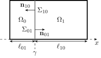
(b) …and its decomposition into $\Omega_{1}$ and $\Omega_{2}$.

Figure 1: Reference computational domain.

Let us solve the following Helmholtz problem on $\Omega$:

$$[left=\empheqlbrace]\operatorname{div}{\operatorname{\mathbf{grad}}{p}}+k^{2}p =g \text{on}~{}\Omega,$$ (1a)

$$p =0 \text{on}~{}\Gamma,$$ (1b)

where $p(x,y)$ is the unknown function, $g(x,y)$ is a known source term and $k\in\mathbb{R}$ is the fixed wavenumber of the Helmholtz problem. Because of its boundary condition, it is obvious that (1) models a cavity problem exhibiting both forward- and back-propagating waves. It is important to stress that for this problem to be well defined, we must assume that $k^{2}$ is not an eigenvalue of (1).

Let us now set up the following optimized non-overlapping Schwarz iterative scheme, indexed by $n$, to solve the cavity Helmholtz problem (1):

$$[left=\empheqlbrace]\operatorname{div}{\operatorname{\mathbf{grad}}{p_{0}^{n+1}}}+k^{2}p_{0}^{n+1} =g \text{on}~{}\Omega_{0},$$ (2a)

$$+\mathbf{n}_{01}\cdot\operatorname{\mathbf{grad}}{p_{0}^{n+1}}+\operatorname{\mathcal{S}}_{01}{(p_{0}^{n+1})} =+\mathbf{n}_{01}\cdot\operatorname{\mathbf{grad}}{p_{1}^{n}}+\operatorname{\mathcal{S}}_{01}{(p_{1}^{n})} \text{on}~{}\Sigma_{01},$$ (2b)

$$p_{0}^{n+1} =0 \text{on}~{}\Gamma,$$ (2c)

$$\operatorname{div}{\operatorname{\mathbf{grad}}{p_{1}^{n+1}}}+k^{2}p_{1}^{n+1} =g \text{on}~{}\Omega_{1},$$ (2d)

$$-\mathbf{n}_{01}\cdot\operatorname{\mathbf{grad}}{p_{1}^{n+1}}+\operatorname{\mathcal{S}}_{10}{(p_{1}^{n+1})} =-\mathbf{n}_{01}\cdot\operatorname{\mathbf{grad}}{p_{0}^{n}}+\operatorname{\mathcal{S}}_{10}{(p_{0}^{n})} \text{on}~{}\Sigma_{10},$$ (2e)

$$p_{1}^{n+1} =0 \text{on}~{}\Gamma,$$ (2f)

where $\operatorname{\mathcal{S}}_{ij}$ is the transmission operator of the optimized Schwarz algorithm at $\Sigma_{ij}$ and $p_{i}^{n}(x,y)$ is the solution at iteration $n$ on domain $\Omega_{i}$. Let us stress that, since the subdomains do not overlap, the following holds true: $\mathbf{n}_{01}=-\mathbf{n}_{10}$. Once the Schwarz algorithm has converged, the solution $p(x,y)$ of the original problem (1) is recovered by concatenating the solutions $p_{0}(x,y)$ and $p_{1}(x,y)$.

In practice, let us note that the above fixed-point scheme is usually recast into the linear system [14]:

$$(\operatorname{\mathcal{I}}-\operatorname{\mathcal{A}})\mathbf{d}=\mathbf{b},$$ (3)

where one application of the operator $\operatorname{\mathcal{A}}$ amounts to one iteration of the fixed-point method with homogeneous Dirichlet boundary conditions, where $\operatorname{\mathcal{I}}$ is the identity operator, where $\mathbf{d}$ concatenates all $\mathbf{n}\cdot\operatorname{\mathbf{grad}}{p}+\operatorname{\mathcal{S}}(p)$ at the interface between the subdomains and where the right hand side vector $\mathbf{b}$ results from the non-homogeneous Dirichlet boundary conditions. This linear system can then be solved with a matrix-free Krylov subspace method such as GMRES.

3 Optimal transmission operator for the rectangular cavity problem with homogeneous Dirichlet boundary conditions

In this section, we will first determine the optimal transmission operators at $\Sigma_{01}$ and $\Sigma_{10}$ of the Schwarz scheme (2) involving the non-overlapping subdomains in Figure 1(b). While this work focuses on non-overlapping decompositions, the impact of an overlap on the optimal transmission operator is also discussed in this section.

3.1 Non-overlapping case

In order to further simplify the problem at hand, let us now assume that the source term $g$ is zero. Obviously, by not imposing a source in our problem the solution $p(x,y)$ is trivially $p=0$ since $k$ is not an eigenvalue. This however does not jeopardize the generality of the results derived in this section.

Let us start by taking the sine Fourier series of $p_{i}^{n}(x,y)$ along the $y$-axis:

$$p_{i}^{n}(x,y)=\sum_{s\in\mathbb{S}}\widehat{p}_{i}^{n}(x,s)\sin(sy),$$ (4)

where the functions $\widehat{p}_{i}^{n}(x,s)$ are the Fourier coefficients and where $s$ is the Fourier variable, whose values are restricted to the set

$$\mathbb{S}=\Big{\{}s\in\mathbb{R}~{}\Big{|}~{}s=m\frac{\pi}{h},\forall m\in\mathbb{N}_{0}\Big{\}}.$$ (5)

Indeed, by restricting $s$ to the set $\mathbb{S}$, the boundary conditions

$$[left=\empheqlbrace]p^{n}_{i}(x,0) =0 \forall x\in\left[-\frac{\ell}{2},+\frac{\ell}{2}\right],$$

$$p^{n}_{i}(x,h) =0 \forall x\in\left[-\frac{\ell}{2},+\frac{\ell}{2}\right],$$

are automatically satisfied. Then, by exploiting decomposition (4), the partial differential equation (2) becomes the following ordinary differential equation:

$$[left=\empheqlbrace]\frac{\partial^{2}\widehat{p}_{0}^{n+1}}{\partial x^{2}}+(k^{2}-s^{2})\widehat{p}_{0}^{n+1} =0 \forall x\in\left[-\frac{\ell}{2},\gamma\right]\text{and}~{}\forall s\in\mathbb{S},$$ (6a)

$$+\frac{\partial\widehat{p}_{0}^{n+1}}{\partial x}+\lambda_{01}\,\widehat{p}_{0}^{n+1} =+\frac{\partial\widehat{p}_{1}^{n}}{\partial x}+\lambda_{01}\,\widehat{p}_{1}^{n} \text{on}~{}x=\gamma~{}\text{and}~{}\forall s\in\mathbb{S},$$ (6b)

$$\widehat{p}_{0}^{n+1} =0 \text{on}~{}x=-\frac{\ell}{2}~{}\text{and}~{}\forall s\in\mathbb{S},$$ (6c)

$$\frac{\partial^{2}\widehat{p}_{1}^{n+1}}{\partial x^{2}}+(k^{2}-s^{2})\widehat{p}_{1}^{n+1} =0 \forall x\in\left[\gamma,+\frac{\ell}{2}\right]\text{and}~{}\forall s\in\mathbb{S},$$ (6d)

$$-\frac{\partial\widehat{p}_{1}^{n+1}}{\partial x}+\lambda_{10}\,\widehat{p}_{1}^{n+1} =-\frac{\partial\widehat{p}_{0}^{n}}{\partial x}+\lambda_{10}\,\widehat{p}_{0}^{n} \text{on}~{}x=\gamma~{}\text{and}~{}\forall s\in\mathbb{S},$$ (6e)

$$\widehat{p}_{1}^{n+1} =0 \text{on}~{}x=+\frac{\ell}{2}~{}\text{and}~{}\forall s\in\mathbb{S},$$ (6f)

where $\lambda_{ij}$ is the Fourier symbol of $\operatorname{\mathcal{S}}_{ij}$. Furthermore, and for simplicity, let us define $P_{i}^{n}(s)$ as:

$$P_{i}^{n}(s)=\widehat{p}_{i}^{n}(0,s).$$ (7)

In order to find the best symbol $\lambda_{ij}$, we need to determine the convergence radius of the iterative scheme (6). This objective can be achieved by following the strategy discussed in [10], which can be summarized as follows.

1. Determine the solutions of (6a) and (6d) with the boundary conditions (6c) and (6f) and the definition (7).

2. Compute $\displaystyle\frac{\partial\widehat{p}_{i}^{n}(x,s)}{\partial x}$ at $x=\gamma$ from the solutions $\widehat{p}_{i}^{n}(x,s)$ found in the previous step.

3. The convergence radius is obtained by simplifying the transmission conditions (6b) and (6e) with the expressions found above.

By following this approach, it can be shown (see A) that the convergence radius $\rho$ of (6) satisfies:

$$\rho^{2}(s)=\frac{\lambda_{01}(s)-\lambda_{01}^{\text{c, dtn}}(s)}{\lambda_{01}(s)+\lambda_{10}^{\text{c, dtn}}(s)}\frac{\lambda_{10}(s)-\lambda_{10}^{\text{c, dtn}}(s)}{\lambda_{10}(s)+\lambda_{01}^{\text{c, dtn}}(s)}=\frac{n_{01}(s)\,n_{10}(s)}{d_{01}(s)\,d_{10}(s)},$$ (8)

where

$$[left={\lambda_{ij}^{\text{c, dtn}}(s)=\empheqlbrace}] \sqrt{k^{2}-s^{2}}\cot\mathopen{}\left[\ell_{ji}\sqrt{k^{2}-s^{2}}\mathclose{}\right] \text{if}~{}s^{2}<k^{2},$$ (9a)

$$1/\ell_{ji} \text{if}~{}s^{2}=k^{2},$$ (9b)

$$\sqrt{s^{2}-k^{2}}\coth\mathopen{}\left[\ell_{ji}\sqrt{s^{2}-k^{2}}\mathclose{}\right] \text{if}~{}s^{2}>k^{2}.$$ (9c)

The best transmission operator $\operatorname{\mathcal{S}}_{ij}^{\text{c, dtn}}$, that is the Dirichlet-to-Neumann map, is thus

$$\operatorname{\mathcal{S}}_{ij}^{\text{c, dtn}}=\operatorname{Op}\mathopen{}\Bigg{\{}\lambda_{ij}^{\text{c, dtn}}\mathclose{}\Bigg{\}}.$$ (10)

3.2 Overlapping case

Let us now assume a partitioning of the domain in Figure 1(a) into two overlapping rectangles, as shown in Figure 2. As suggested by this figure, we define $\ell_{01}$ (resp. $\ell_{10}$) as the length of $\Omega_{0}$ (resp. $\Omega_{1}$) including the overlap and $\ell_{01}^{\prime}$ (resp. $\ell_{10}^{\prime}$) as the length of $\Omega_{0}$ (resp. $\Omega_{1}$) without the overlap. By following the same strategy as in the non-overlapping case, but taking into account that $\Sigma_{01}$ and $\Sigma_{10}$ have now different locations, the convergence radius $\rho^{\text{overlap}}$ of the overlapping variant of (6) reads (see B):

$$[left={(\rho^{\text{overlap}})^{2}=\empheqlbrace}] \left(\frac{\lambda_{01}-\alpha\cot(\alpha\ell_{10}^{\prime})}{\lambda_{01}+\alpha\cot(\alpha\ell_{01})}\frac{\lambda_{10}-\alpha\cot(\alpha\ell_{01}^{\prime})}{\lambda_{10}+\alpha\cot(\alpha\ell_{10})}\right)\left(\frac{\sin(\alpha\ell_{10}^{\prime})}{\sin(\alpha\ell_{10})}\frac{\sin(\alpha\ell_{01}^{\prime})}{\sin(\alpha\ell_{01})}\right) \text{if}~{}s^{2}<k^{2},$$ (11a)

$$\left(\frac{\lambda_{01}-(\ell_{10}^{\prime})^{-1}}{\lambda_{01}+(\ell_{01})^{-1}}\frac{\lambda_{10}-(\ell_{01}^{\prime})^{-1}}{\lambda_{10}+(\ell_{10})^{-1}}\right)\left(\frac{\ell_{10}^{\prime}}{\ell_{10}}\frac{\ell_{01}^{\prime}}{\ell_{01}}\right) \text{if}~{}s^{2}=k^{2},$$ (11b)

$$\left(\frac{\lambda_{01}-\alpha\coth(\alpha\ell_{10}^{\prime})}{\lambda_{01}+\alpha\coth(\alpha\ell_{01})}\frac{\lambda_{10}-\alpha\coth(\alpha\ell_{01}^{\prime})}{\lambda_{10}+\alpha\coth(\alpha\ell_{10})}\right)\left(\frac{\sinh(\alpha\ell_{10}^{\prime})}{\sinh(\alpha\ell_{10})}\frac{\sinh(\alpha\ell_{01}^{\prime})}{\sinh(\alpha\ell_{01})}\right) \text{if}~{}s^{2}>k^{2},$$ (11c)

where

$$[left={\alpha(s)=\empheqlbrace}] -\jmath\sqrt{k^{2}-s^{2}} \text{if}~{}s^{2}<k^{2},$$ (12a)

$$0 \text{if}~{}s^{2}=k^{2},$$ (12b)

$$\sqrt{s^{2}-k^{2}} \text{if}~{}s^{2}>k^{2}.$$ (12c)

A few conclusions can be drawn from the above expressions. Firstly, it is clear from (11) that the optimal transmission operator writes

$$[left={\lambda_{ij}^{\text{c, dtn, overlap}}(s)=\empheqlbrace}] \sqrt{k^{2}-s^{2}}\cot\mathopen{}\left[\ell_{ji}^{\prime}\sqrt{k^{2}-s^{2}}\mathclose{}\right] \text{if}~{}s^{2}<k^{2},$$ (13a)

$$1/\ell_{ji}^{\prime} \text{if}~{}s^{2}=k^{2},$$ (13b)

$$\sqrt{s^{2}-k^{2}}\coth\mathopen{}\left[\ell_{ji}^{\prime}\sqrt{s^{2}-k^{2}}\mathclose{}\right] \text{if}~{}s^{2}>k^{2},$$ (13c)

that is $\lambda_{ij}^{\text{c, dtn, overlap}}(s)$ is equal to $\lambda_{ij}^{\text{c, dtn}}(s)$, up to the substitution $\ell_{ji}\rightarrow\ell_{ji}^{\prime}$. Secondly, it is easy to notice that when there is no overlap, it holds that $\ell_{ji}=\ell_{ji}^{\prime}$ and the non-overlapping case is recovered. Thirdly and most importantly, it is obvious that an overlap does not necessarily improve the convergence radius $\rho^{\text{overlap}}$ unlike for the unbounded case [14], since when $s^{2}<k^{2}$ (i.e. propagating modes) the term involving the $\sin$ functions in (11a) exhibits poles and oscillates with respect to the size of the overlap. Nonetheless, the term with the $\sinh$ functions in (11c) introduces a damping proportional to the overlap, as in the unbounded case, but only when $s^{2}>k^{2}$ (i.e. evanescent modes).

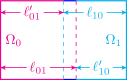
Figure 2: Overlapping partitioning of the computational domain.

4 Some local transmission operators for the cavity problem

In this section, we discuss some local transmission operators based on the Fourier symbol (9).

4.1 Zeroth-order transmission condition

A zeroth-order transmission condition (OO0^c) can easily be constructed by approximating the symbol of the $\operatorname{DtN}$ map with the constant term of its Taylor series expansion around $s=0$. For the considered cavity setting, we obtain:

$$\lambda_{ij}^{\text{c, dtn}}(s)\approx\lambda_{ij}^{\text{c, oo0}}(s)=k\cot(k\ell_{ji})$$ (14)

and the OO0^c transmission condition reads

$$\operatorname{\mathcal{S}}_{ij}^{\text{c, oo0}}=k\cot(k\ell_{ji}).$$ (15)

As such, this operator exhibits a rather poor behavior. Indeed, the denominator of the convergence radius (8) involves terms of the form

$$d_{ij}(s)=\lambda_{ij}(s)+\lambda_{ji}^{\text{c, dtn}}(s),$$ (16)

which can change their sign multiple times when $s^{2}<k^{2}$, since $\lambda_{ji}^{\text{c, dtn}}$ is nothing but a cotangent and $\lambda_{ij}^{\text{c, oo0}}$ is constant. Consequently, it is possible that $d_{ij}\approx 0$ for some $s\in\mathbb{S}$, leading to a very large convergence radius. In the worst case scenario, one can also have $d_{ij}=0$ for some $s\in\mathbb{S}$ and the problem becomes ill-posed. Regularization procedures for preventing this behavior are further discussed in sections 4.5 and 4.6.

4.2 Truncated Mittag-Leffler expansion based transmission condition

In order to improve the performance of the above OO0^c transmission condition for cavity problem, we need a condition whose symbol is a better approximation of $\lambda_{ij}^{\text{c, dtn}}$. To this end, an option is to exploit the Mittag-Leffler [20] expansion of $\cot(z)$ according to its poles, leading to the following partial fraction decomposition [20]:

$$z\cot(az)=\frac{1}{a}\left(1+2\sum_{n=1}^{\infty}\frac{z^{2}}{z^{2}-\left(\frac{n\pi}{a}\right)^{2}}\right),$$ (17)

that can be exploited to expand the symbol of the $\operatorname{DtN}$ map as

$$\lambda_{ij}^{\text{c, dtn}}(s)=\frac{1}{\ell_{ji}}\left(1+2\sum_{n=1}^{\infty}\frac{1-\frac{s^{2}}{k^{2}}}{1-\left(\frac{n\pi}{k\ell_{ji}}\right)^{2}-\frac{s^{2}}{k^{2}}}\right).$$ (18)

This symbol can hence be localized by truncating the series up to the $N$^th term, enabling us to form a $N$-term truncated Mittag-Leffler expansion based (ML^c) transmission condition:

$$\operatorname{\mathcal{S}}_{ij}^{\text{c, ml($N$)}}=\frac{1}{\ell_{ji}}\left\{1+2\sum_{n=1}^{N}\Bigg{[}1+\frac{\operatorname{div}_{\Sigma_{ij}}\operatorname{\mathbf{grad}}_{\Sigma_{ij}}}{k^{2}}\Bigg{]}\Bigg{[}1-\Bigg{(}\frac{n\pi}{k\ell_{ji}}\Bigg{)}^{2}+\frac{\operatorname{div}_{\Sigma_{ij}}\operatorname{\mathbf{grad}}_{\Sigma_{ij}}}{k^{2}}\Bigg{]}^{-1}\right\}.$$ (19)

As increasing the number of terms in this expansion makes the transmission condition arbitrarily precise, the poor convergence rate of the previous OO0^c operator can be alleviated. This comes however at the cost of $N$ auxiliary computations to account for the $N$ inverse operations appearing in (19) [11]. For this reason, it is desirable to devise an approximation of $\lambda_{ij}^{\text{c, dtn}}(s)$ with a limited number of auxiliary terms. Let us also mention that while the above operator has been developed for a one-dimensional interface, it can be used as well with a two-dimensional one, as shown in section 9 for instance.

4.3 Padé approximant based transmission condition

A Padé rational approximation exhibits usually a good convergence rate with respect to its order $[M/N]$, where $M$ (resp. $N$) denotes the order of the numerator (resp. denominator). One can construct it by exploiting the continued fraction expansion of the function to approach [21]. By taking the reciprocal of the continued fraction expansion of the tangent function [22], we have:

$$z\cot(z)=1-\cfrac{z^{2}}{3-\cfrac{z^{2}}{7-\cfrac{z^{2}}{9-\dots}}}=b_{0}+\cfrac{a_{1}}{b_{1}+\cfrac{a_{2}}{b_{2}+\cfrac{a_{3}}{b_{3}+\dots}}},$$ (20)

where

$$[left=\empheqlbrace]b_{n} =2n+1 \forall{}n\geq 0,$$

$$a_{n} =-z^{2} \forall{}n\geq 1.$$

The Padé approximant can then be determined from the following recurrence formula [21]:

$$\frac{A_{m}}{B_{l}}=\frac{b_{m}A_{m-1}+a_{m}A_{m-2}}{b_{l}B_{l-1}+a_{l}B_{l-2}}\qquad\forall{}m\geq{}2~{}\text{and}~{}\forall{}l\geq{}2,$$ (22)

with

$$\begin{array}[]{c@{\quad\text{and}\quad}c}\left\{\begin{array}[]{r@{~}c@{~}l}A_{0}~{}&=\hfil~{}&b_{0},\\ B_{0}~{}&=\hfil~{}&1,\end{array}\right.&\left\{\begin{array}[]{r@{~}c@{~}l}A_{1}~{}&=\hfil~{}&b_{1}b_{0}+a_{1},\\ B_{1}~{}&=\hfil~{}&b_{1}.\end{array}\right.\end{array}$$

That is, we have for the $z\cot(z)$ function:

$$\begin{array}[]{c@{\quad\text{and}\quad}c@{\quad\text{and}\quad}c}\left\{\begin{array}[]{r@{~}c@{~}l}A_{0}~{}&=\hfil~{}&1,\\ B_{0}~{}&=\hfil~{}&1,\end{array}\right.&\left\{\begin{array}[]{r@{~}c@{~}l}A_{1}~{}&=\hfil~{}&3-z^{2},\\ B_{1}~{}&=\hfil~{}&3,\end{array}\right.&\left\{\begin{array}[]{r@{~}c@{~}l}A_{m}~{}&=\hfil~{}&(2m+1)A_{m-1}-z^{2}A_{m-2},\\ B_{l}~{}&=\hfil~{}&(2l+1)B_{l-1}-z^{2}B_{l-2}.\end{array}\right.\end{array}$$ (23)

Starting from this recurrence formula and choosing $l=m$, we can devise a $N$-term decomposition of the form

$$z\cot(z)\approx\frac{A_{N}}{B_{N}}=\tilde{C}_{0}+\sum_{i=0}^{N}\frac{\tilde{A}_{i}}{z^{2}-\tilde{B}_{i}}.$$ (24)

However, compared with the unbounded case where the coefficients of the Padé approximant of the $\operatorname{DtN}$ map are known analytically and exploited to construct the PADE^u operator [11], no closed form formulae were found for the coefficients $\tilde{C}_{0}$, $\tilde{A}_{i}$ and $\tilde{B}_{i}$ of (24). Nevertheless, those can be computed numerically by

1. performing a polynomial long division of $A_{N}/B_{N}$, that is $A_{N}=\tilde{C}_{0}B_{N}+R$,

2. computing the poles $\tilde{B}_{i}$ of $R/B_{N}$ and

3. determining the residues $\tilde{A}_{i}$ of $R/B_{N}$.

The numerically demanding part of this approach is the calculation of the poles of $R/B_{N}$, i.e. the zeros of $B_{N}$, which requires arbitrary precision arithmetic as the coefficients of the monomials appearing in $B_{N}$ can be vary large.

In this work, this is achieved with the MPSolve library [23]. Within that framework, it takes less than 5 minutes to compute the $\tilde{C}_{0}$, $\tilde{A}_{i}$ and $\tilde{B}_{i}$ coefficients in the very large case of $N=1024$ for instance. Of course, these coefficients can be pre-computed and tabulated for various values of $N$ and the actual transmission condition recovered with the change of variable $z=\ell_{ji}\sqrt{k^{2}-s^{2}}$ (see paragraph below). For illustration purposes, the Padé coefficients are presented in Table 1 for $N\in[1,4]$.

$N$	$\tilde{C}_{0}$	$\tilde{A}_{i}$	$\tilde{B}_{i}$
$1$	$6.00\times{}10^{0}$	$7.50\times{}10^{1}$	$1.50\times{}10^{1}$
$2$	$1.50\times{}10^{1}$	$2.05\times{}10^{1}$	$9.94\times{}10^{0}$
		$1.13\times{}10^{3}$	$9.51\times{}10^{1}$
$3$	$2.80\times{}10^{1}$	$1.97\times{}10^{1}$	$9.87\times{}10^{0}$
		$1.09\times{}10^{2}$	$4.20\times{}10^{1}$
		$7.31\times{}10^{3}$	$3.26\times{}10^{2}$

    $N$ $\tilde{C}_{0}$ $\tilde{A}_{i}$ $\tilde{B}_{i}$ $4$ $4.50\times{}10^{1}$ $1.97\times{}10^{1}$ $9.87\times{}10^{0}$ $8.03\times{}10^{1}$ $3.96\times{}10^{1}$ $4.03\times{}10^{2}$ $1.06\times{}10^{2}$ $3.02\times{}10^{4}$ $8.35\times{}10^{2}$

Table 1: Padé coefficients $\tilde{C}_{0}$, $\tilde{A}_{i}$ and $\tilde{B}_{i}$ for $N\in[1,4]$.

Capitalizing on the above development, we can now devise a new approximation (PADE^c) of $\lambda_{ij}^{\text{c, dtn}}$ of the form

$$\lambda_{ij}^{\text{c, dtn}}(s)\approx\lambda_{ij}^{\text{c, pade($N$)}}(s)=\frac{1}{\ell_{ji}}\left(\tilde{C}_{0}+\sum_{n=1}^{N}\frac{\tilde{A}_{n}}{\Big{(}k\ell_{ji}\Big{)}^{2}\Big{(}1-\frac{s^{2}}{k^{2}}\Big{)}-\tilde{B}_{n}}\right),$$ (25)

by exploiting the change of variable $z=\ell_{ji}\sqrt{k^{2}-s^{2}}$. The operator associated with this symbol then reads:

$$\operatorname{\mathcal{S}}_{ij}^{\text{c, pade($N$)}}=\frac{1}{\ell_{ji}}\left\{\tilde{C}_{0}+\sum_{n=1}^{N}\tilde{A}_{n}\Bigg{[}\Bigg{(}k\ell_{ji}\Bigg{)}^{2}\Bigg{(}1+\frac{\operatorname{div}_{\Sigma_{ij}}\operatorname{\mathbf{grad}}_{\Sigma_{ij}}}{k^{2}}\Bigg{)}-\tilde{B}_{n}\Bigg{]}^{-1}\right\}.$$ (26)

As in the truncated Mittag-Leffler expansion case, the above operator has been developed for a one-dimensional interface, but can be used as well with a two-dimensional one, as shown in section 9 for instance.

Before concluding this subsection, let us mention that the truncated Mittag-Leffler expansion of $z\cot(z)$ is related to its Padé approximant in the following way: the square-root of the $i$^th pole appearing in (24) is converging towards $(i+1)\pi$, i.e. the $(i+1)$^th pole of $z\cot(z)$ appearing in (17), for a fixed value of $i$ and as $N$ increases. Formally, we have that

$$\lim_{N\to\infty}\sqrt{\tilde{B}_{i}}=(i+1)\pi\quad\forall i\geq 0,$$ (27)

as show in Figure 3 for the first six poles.

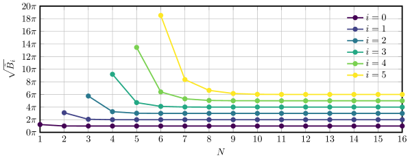
Figure 3: Convergence of the square-root of the $i$^th pole of the Padé approximant with $N$.

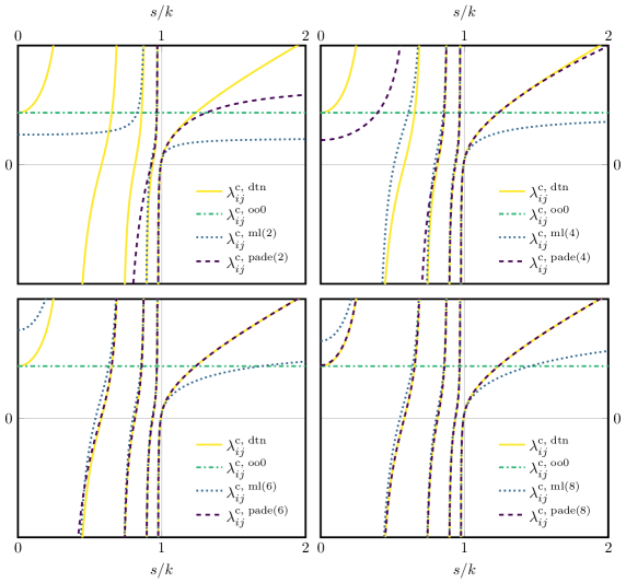
Figure 4: Approximation quality of the different transmission operators in a one-dimensional setting with $\ell/\lambda_{w}=4.3$ and two subdomains of equal size (arbitrary values for the y-axis, only the zero is shown to highlight the sign changes).

4.4 Quality of the transmission operators in the one-dimensional case

As the $\operatorname{DtN}$ and the three transmission operators discussed above are purely real, they reduce to a simple real function in the one-dimensional case, allowing a simple graphical comparison, as suggested in Figure 4. For clarity reasons, this figure is restricted to a relatively low frequency problem with a ratio $\ell/\lambda_{w}=4.3$, where $\lambda_{w}=2\pi/k$ is the wavelength, and two subdomains of equal size. Nonetheless, the discussion below remains general.

To start with, it is clear that OO0^c is a quite poor approximation of the $\operatorname{DtN}$, as it obviously cannot capture its oscillations and its poles. It is also apparent that changing the expansion point of the Taylor series (here $s=0$, as a recall) will not improve the situation.

On the other hand, both ML^c and PADE^c are able to capture the oscillation and poles of the $\operatorname{DtN}$, at least for a sufficiently high value of $N$. Those approximations exhibit however major differences, which are summarized in what follows.

• For the evanescent modes (i.e. when $s/k>1$), the convergence of $\lambda_{ij}^{\text{c, ml($N$)}}$ towards $\lambda_{ij}^{\text{c, dtn}}$ as $N$ increases is quite slow, at least when compared with $\lambda_{ij}^{\text{c, pade($N$)}}$. Let us mention that in the unbounded case, $\lambda_{ij}^{\text{u, pade($N$)}}$ is known to perform well when $s/k>1$. This aspect will be further discussed in section 6.

• For the non-evanescent modes (i.e. when $s/k<1$), each pole introduced by $\lambda_{ij}^{\text{c, ml($N$)}}$ coincides, by construction, with a pole of $\lambda_{ij}^{\text{c, dtn}}$. Thus for low values of $N$ where all the poles of $\lambda_{ij}^{\text{c, dtn}}$ are not yet present, $\lambda_{ij}^{\text{c, ml($N$)}}$ leads to better approximations of $\lambda_{ij}^{\text{c, dtn}}$ than $\lambda_{ij}^{\text{c, pade($N$)}}$, at least when restricting $s/k$ to the range spanned by the first and last poles of $\lambda_{ij}^{\text{c, ml($N$)}}$. Conversely, for higher values of $N$, the approximation given by $\lambda_{ij}^{\text{c, pade($N$)}}$ is clearly the best one.

To conclude this subsection, let us also note that the approximation is better as $s/k$ tends to $1$ for both $\lambda_{ij}^{\text{c, ml($N$)}}$ and $\lambda_{ij}^{\text{c, pade($N$)}}$.

4.5 Regularization with a constant imaginary part

As already mentioned earlier, the zeroth-order transmission condition optimized for the cavity problem can lead to an ill-posed problem when one of the $d_{ij}(s)$ terms in the denominator of the convergence radius (8) equals (or is sufficiently close to) zero. This problem is however not peculiar to the OO0^c condition and affects the ML^c and PADE^c ones as well, requiring therefore a regularization procedure.

The most straightforward and simple strategy to regularize the OO0^c, ML^c and PADE^c conditions is to exploit the fact that those operators are purely real-valued. Consequently, by adding a purely imaginary part, the $d_{ij}(s)$ terms can be pushed away from zero and the convergence radius $\rho(s)$ can be guaranteed to be well defined. Formally, the regularized OO0^c, ML^c and PADE^c operators read

$$\operatorname{\mathcal{S}}_{ij}^{\text{c, oo0/ml($N$)/pade($N$), r($\chi$)}}=\operatorname{\mathcal{S}}_{ij}^{\text{c, oo0/ml($N$)/pade($N$)}}+\jmath\chi k,$$ (28)

where $\chi\in\mathbb{R}$ is the regularization parameter. Numerical experiments showing the impact of this regularization approach are further discussed in sections 7 and 8.

4.6 Regularization by mixing operators optimized for cavity and unbounded problems

The above regularization is in some sense suboptimal as it acts on all $s\in\mathbb{S}$, while regularization is required only in the $s^{2}<k^{2}$ case. A more selective approach can be achieved by exploiting the PADE^u operator. Indeed, assuming a sufficiently high value of $N$ and an appropriate rotation of the branch cut [24] of PADE^u, the latter exhibits the following properties [24]:

1. it is approximately imaginary when $s^{2}<k^{2}$,

2. it is approximately real when $s^{2}>k^{2}$ and

3. it is a good approximation of the $\operatorname{DtN}$ map when $s^{2}>k^{2}$ (see discussion in section 6).

Therefore, a regularized operator can be constructed by combining either the OO0^c, the ML^c or the PADE^c operator with the PADE^u one in a convex way. These new operators will be further referred to as mixed operator and write

$$\operatorname{\mathcal{S}}_{ij}^{\text{m($\varepsilon,M$), oo0/ml($N$)/pade($N$)}}=\varepsilon\operatorname{\mathcal{S}}_{ij}^{\text{c, oo0/ml($N$)/pade($N$)}}+(1-\varepsilon)\operatorname{\mathcal{S}}_{ij}^{\text{u, pade($M$)}},$$ (29)

where $\varepsilon\in]0,1[$ denotes the regularization parameter of the mixed formulation.

4.7 Estimate for the minimum number of auxiliary unknowns

Given the ML^c and PADE^c transmission conditions, one question naturally arises: how many auxiliary terms should be selected? In order to answer this question, one could opt for the following criterion: the number of auxiliary terms $N$ should at least be equal to the number of poles of $\lambda_{ij}^{\text{c, dtn}}$, as it seems legitimate to assume that the behavior of $\lambda_{ij}^{\text{c, dtn}}$ is driven by its poles in the range $s^{2}<k^{2}$.

Given the Mittag-Leffler expansion of $\lambda_{ij}^{\text{c, dtn}}$, it is clear that the poles must satisfy

$$s^{2}=k^{2}-\left(\frac{n\pi}{\ell_{ij}}\right)^{2}\quad\forall{}n>0,$$ (30)

which implies that

$$k^{2}-\left(\frac{n\pi}{\ell_{ij}}\right)^{2}>0$$ (31)

and thus

$$0<n<2\frac{\ell_{ij}}{\lambda_{w}},$$ (32)

since $k$, $n$ and $\ell_{ij}$ are positive by construction.

Therefore, according to the pole criterion stated above, the minimum number of terms $N_{\text{min}}^{\text{poles}}$ for localizing $\lambda_{ij}^{\text{c, dtn}}$ is

$$N_{\text{min}}^{\text{pole}}=\left\lceil 2\frac{\ell_{ij}}{\lambda_{w}}\right\rceil$$ (33)

and depends on the size of the subdomains and on the wavelength. As discussed further in section 7.4, this criterion seems however pessimistic, as lower values of $N_{\text{min}}^{\text{pole}}$ provide already acceptable results.

5 Generalizations

The transmission operators detailed in the pervious section are restricted to the very particular case of a cavity with Dirichlet boundary conditions divided into two subdomains. In order to generalize this setting, we discuss in section the cases of many subdomains in a one-dimensional partitioning and of Neumann boundary conditions.

5.1 One-dimensional partitioning with more than two subdomains

Let us start with the one-dimensional partitioning of the computational domain into $D$ subdomains, as shown in Figure 5(a). In such a one-dimensional domain decomposition, the physical meaning of the $\ell_{ji}$ coefficient appearing in $\lambda_{ij}^{\text{c, dtn}}(s)$ must be clarified. In the two subdomains case, the $\ell_{ji}$ coefficients represents the distance between $\Sigma_{ij}$ and the reflecting wall located in the $\mathbf{n}_{ij}$ direction. This interpretation can be directly applied to the $D$ subdomains case to define the $\ell_{ji}$ coefficients, as shown in Figure 5(b) for the $D=3$ case.

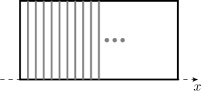
(a) Partitioning into $D$ subdomains.

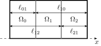
(b) Definition of $\ell_{ji}$ (here for $D=3$ subdomains).

Figure 5: One-dimensional partitioning of the rectangular cavity.

5.2 Neumann boundary conditions

So far, we considered only the situation where the reflecting wall associated with $\operatorname{\mathcal{S}}_{ij}$ is implemented with an homogeneous Dirichlet boundary condition, i.e. a soft-wall condition. In the case of an homogeneous Neumann boundary condition, i.e. a hard-wall condition, the following $\operatorname{DtN}$ map is obtained:

$$[left={\lambda_{ij}^{\text{c, dtn, neumann}}(s)=\empheqlbrace}] -\sqrt{k^{2}-s^{2}}\tan\mathopen{}\left[\ell_{ji}\sqrt{k^{2}-s^{2}}\mathclose{}\right] \text{if}~{}s^{2}<k^{2},$$ (34a)

$$0 \text{if}~{}s^{2}=k^{2},$$ (34b)

$$\sqrt{s^{2}-k^{2}}\tanh\mathopen{}\left[\ell_{ji}\sqrt{s^{2}-k^{2}}\mathclose{}\right] \text{if}~{}s^{2}>k^{2},$$ (34c)

by following the same strategy as in section 3. It is worth stressing the similarities between (9) and (34). This $\operatorname{DtN}$ map can then be localized using the previously presented approaches and a OO0^c, ML^c or PADE^c transmission condition can be devised. In this regard, let us note that the Mittag-Leffler expansion of $\tan(z)$ reads [25]

$$z\tan(az)=-\frac{2}{a}\sum_{n=0}^{\infty}\frac{z^{2}}{z^{2}-\left[\frac{(n+\frac{1}{2})\pi}{a}\right]^{2}}$$ (35)

and its continued fraction expansion has the following form [22]:

$$z\tan(z)=\cfrac{z^{2}}{1-\cfrac{z^{2}}{3-\cfrac{z^{2}}{5-\dots}}}=b_{0}+\cfrac{a_{1}}{b_{1}+\cfrac{a_{2}}{b_{2}+\cfrac{a_{3}}{b_{3}+\dots}}}.$$ (36)

These results are given here for the sake of completeness and will not be further discussed in this work.

6 Operators optimized for unbounded problems without obstacles in a cavity context

In this section we derive some estimates on the performance of operators optimized for unbounded problems without obstacles when used in a cavity problem. In particular, i) we first compare the $\operatorname{DtN}$ operator related to an unbounded problem without obstacles $\operatorname{\mathcal{S}}_{ij}^{\text{u, dtn}}$ with its cavity counter part $\operatorname{\mathcal{S}}_{ij}^{\text{c, dtn}}$, then ii) we discuss the convergence radius of the OS scheme when using $\operatorname{\mathcal{S}}_{ij}^{\text{u, dtn}}$ as a transmission operator for the rectangular cavity problem (1), as well as iii) the particular case of the optimized order 0 operator (OO0^u) [8].

6.1 Dirichlet-to-Neumann operators

Let us consider the following Helmholtz problem without obstacles:

$$[left=\empheqlbrace]\operatorname{div}{\operatorname{\mathbf{grad}}{p}}+k^{2}p =g\quad\text{on}~{}\mathbb{R}^{2},$$ (37a)

$$\lim_{r\to\infty}\sqrt{r}\left(\frac{\partial p}{\partial r}-\jmath{}kp\right) =0,$$ (37b)

where $r^{2}=x^{2}+y^{2}$. In this case, it can be shown that the optimal transmission operator $\operatorname{\mathcal{S}}_{ij}^{\text{u, dtn}}$ for solving this problem with an OS scheme is [11]:

$$\operatorname{\mathcal{S}}_{ij}^{\text{u, dtn}}=\operatorname{Op}\mathopen{}\Big{(}\lambda_{ij}^{\text{u, dtn}}\mathclose{}\Big{)}=-\jmath{}k\sqrt{1+\frac{\operatorname{div}_{\Sigma_{ij}}\operatorname{\mathbf{grad}}_{\Sigma_{ij}}}{k^{2}}},$$ (38)

where

$$\lambda_{ij}^{\text{u, dtn}}=-\jmath{}k\sqrt{1-\frac{s^{2}}{k^{2}}}.$$ (39)

By comparing (39) and (9), it is easy to realize that

$$[left={\lambda_{ij}^{\text{c, dtn}}(s)-\lambda_{ij}^{\text{u, dtn}}(s)=\empheqlbrace}] \sqrt{k^{2}-s^{2}}\cot\mathopen{}\left[\ell_{ji}\sqrt{k^{2}-s^{2}}\mathclose{}\right]+\jmath{}\sqrt{k^{2}-s^{2}} \text{if}~{}s^{2}<k^{2},$$ (40a)

$$1/\ell_{ji} \text{if}~{}s^{2}=k^{2},$$ (40b)

$$\sqrt{s^{2}-k^{2}}\coth\mathopen{}\left[\ell_{ji}\sqrt{s^{2}-k^{2}}\mathclose{}\right]-\sqrt{s^{2}-k^{2}} \text{if}~{}s^{2}>k^{2}.$$ (40c)

Interestingly, by exploiting the definition of the hyperbolic cotangent [22], the case $s^{2}>k^{2}$ can be further simplified into

$$\lambda_{ij}^{\text{c, dtn}}(s)-\lambda_{ij}^{\text{u, dtn}}(s) =\sqrt{s^{2}-k^{2}}\coth\mathopen{}\left[\ell_{ji}\sqrt{s^{2}-k^{2}}\mathclose{}\right]-\sqrt{s^{2}-k^{2}}$$

$$=\sqrt{s^{2}-k^{2}}\left(\frac{\exp\mathopen{}\left(2\ell_{ji}\sqrt{s^{2}-k^{2}}\mathclose{}\right)+1}{\exp\mathopen{}\left(2\ell_{ji}\sqrt{s^{2}-k^{2}}\mathclose{}\right)-1}-1\right)$$

$$=\frac{2}{\exp\mathopen{}\left(2\ell_{ji}\sqrt{s^{2}-k^{2}}\mathclose{}\right)-1}\sqrt{s^{2}-k^{2}} \text{if}~{}s^{2}>k^{2},$$ (41)

which yields:

$$\lim_{s\to\infty}\lambda_{ij}^{\text{c, dtn}}(s)-\lambda_{ij}^{\text{u, dtn}}(s)=0.$$ (42)

In other words, for the case $s^{2}>k^{2}$, the symbol $\lambda_{ij}^{\text{u, dtn}}(s)$ is converging towards $\lambda_{ij}^{\text{c, dtn}}(s)$ as $s$ grows. Furthermore, as the difference between both symbols is decreasing exponentially, $\lambda_{ij}^{\text{u, dtn}}(s)$ is an excellent approximation of $\lambda_{ij}^{\text{c, dtn}}(s)$ when $s^{2}>k^{2}$.

Regarding the case $s^{2}<k^{2}$, as the codomains of $\lambda_{ij}^{\text{u, dtn}}(s)$ (which is purely imaginary) and $\lambda_{ij}^{\text{c, dtn}}(s)$ (which is purely real) do not match, the expression in (40a) cannot be further simplified. For illustration purposes, the graphs of $\lambda_{ij}^{\text{u, dtn}}$ and $\lambda_{ij}^{\text{c, dtn}}$ are depicted in Figure 6 for different values of $k$ ($\Re$ and $\Im$ are respectively denoting the real and imaginary part functions).

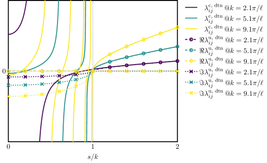
Figure 6: Graphs of $\lambda_{ij}^{\text{u, dtn}}(s/k)$ and $\lambda_{ij}^{\text{c, dtn}}(s/k)$ for different values of $k$ (arbitrary values for the y-axis, only the zero is shown to highlight the sign changes).

6.2 Best convergence radius

We already know from the previous section that $\lambda_{ij}^{\text{u, dtn}}(s)$ is a good approximation of $\lambda_{ij}^{\text{c, dtn}}(s)$ when $s^{2}>k^{2}$, that is for evanescent modes. For this reason, local approximations of $\lambda_{ij}^{\text{u, dtn}}$ are legitimate, yet suboptimal, candidates for approximating $\lambda_{ij}^{\text{c, dtn}}$.

In terms of convergence radius, as defined in (8), it is easy to show that

$$[left={\rho^{2}(s)=\empheqlbrace}] \frac{\jmath-\cot\mathopen{}\left[\ell_{ji}\sqrt{k^{2}-s^{2}}\mathclose{}\right]}{\jmath+\cot\mathopen{}\left[\ell_{ij}\sqrt{k^{2}-s^{2}}\mathclose{}\right]}\frac{\jmath-\cot\mathopen{}\left[\ell_{ij}\sqrt{k^{2}-s^{2}}\mathclose{}\right]}{\jmath+\cot\mathopen{}\left[\ell_{ji}\sqrt{k^{2}-s^{2}}\mathclose{}\right]} \text{if}~{}s^{2}<k^{2},$$ (43a)

$$1 \text{if}~{}s^{2}=k^{2},$$ (43b)

$$\frac{1-\coth\mathopen{}\left[\ell_{ji}\sqrt{s^{2}-k^{2}}\mathclose{}\right]}{1+\coth\mathopen{}\left[\ell_{ij}\sqrt{s^{2}-k^{2}}\mathclose{}\right]}\frac{1-\coth\mathopen{}\left[\ell_{ij}\sqrt{s^{2}-k^{2}}\mathclose{}\right]}{1+\coth\mathopen{}\left[\ell_{ji}\sqrt{s^{2}-k^{2}}\mathclose{}\right]} \text{if}~{}s^{2}>k^{2},$$ (43c)

and

$$[left={\mathinner{\!\left\lvert\rho(s)\right\rvert}=\empheqlbrace}] 1 \text{if}~{}s^{2}\leq{}k^{2},$$ (44a)

$$\exp\mathopen{}\left(-\ell\sqrt{s^{2}-k^{2}}\mathclose{}\right) \text{if}~{}s^{2}>k^{2},$$ (44b)

when $\lambda_{ij}^{\text{c, dtn}}$ is approximated with $\lambda_{ij}^{\text{u, dtn}}$. For this reason, the transmission operators that are good approximations of $\lambda_{ij}^{\text{u, dtn}}$, such that the optimized order 2 (OO2^u) [10] or the $N$-term Padé-localized (PADE^u) [11] operators, should exhibit a convergence radius close to (44). In other words, those local operators should exhibit a slow convergence for the propagating modes ($s^{2}<k^{2}$) and a fast convergence for the evanescent ones ($s^{2}>k^{2}$).

6.3 Particular case of the optimized order 0 operator

Before concluding this subsection, it is worth mentioning that in the case of the OO0^u operator, we have that $\lambda_{ij}^{\text{u, oo0}}=-\jmath{}k$ and therefore

$$\mathinner{\!\left\lvert\rho(s)\right\rvert}=1.$$ (45)

7 Numerical validation and comparison between the different operators

In this section we analyze the performance of the different transmission conditions developed in section 4 and compare them with the operators of section 6. To this end, we consider the rectangular cavity shown in Figure 1(a) and solve the time-harmonic Helmholtz equation over $\Omega$ with the following boundary conditions imposed on $\Gamma$:

$$[left=\empheqlbrace]p =0 \text{on}~{}\Gamma_{w}\cup\Gamma_{r},$$ (46a)

$$p =\displaystyle\sum_{m=1}^{K}\sin\left(m\frac{\pi}{h}y\right) \text{on}~{}\Gamma_{l},$$ (46b)

where $K$ designates the number of modes used to excite the cavity. This Helmholtz problem is then decomposed into $D$ subdomains of equal size and solved with an optimized Schwarz scheme combined with a GMRES algorithm without restart. Let us mention as well that the software implementation relies on the GmshDDM and GmshFEM [26] frameworks and exploits a finite element (FE) discretization of the subproblems. In the case of the $\operatorname{\mathcal{S}}_{ij}^{\text{c, pade($N$)}}$ and $\operatorname{\mathcal{S}}_{ij}^{\text{c, ml($N$)}}$ operators, the FE variational formulations involve auxiliary unknowns for the treatment of the inverse operation, as proposed in [11]. However, let us note that since the new transmission operators are not symmetric, i.e. $\operatorname{\mathcal{S}}_{ij}^{\text{c, oo0/ml($N$)/pade($N$)}}\neq\operatorname{\mathcal{S}}_{ji}^{\text{c, oo0/ml($N$)/pade($N$)}}$, the amount of auxiliary fields must be doubled.

As the novel transmission conditions involve operators oscillating rapidly in a wide range, the finite precision arithmetic aspects of the linear solver must be treated with care. In this regard, the orthogonalization step of the GMRES solver is critical and the modified version of the Gram-Schmidt algorithm [27, 28] is required for convergence. Concerning the software implementation, the linear solvers of the PETSc [29] (GMRES) and MUMPS [30] (LU factorization) libraries are used.

Unless stated otherwise, the cavity has an aspect ratio of $\ell/h=2$ and a length-to-wavelength ratio of $\ell/\lambda_{w}=\frac{157.085}{2\pi}\approx 25.001$. This configuration allows $25$ non-evanescent modes and is excited with the $K=50$ first modes. The geometry is discretized with a mesh consisting of $8$ triangular elements per wavelength and the subproblems are discretized with an FE method of order $4$. The stopping criterion of the GMRES solver is set to a relative tolerance decrease of $\mathinner{\!\left\lVert\mathbf{r}_{i}\right\rVert}/\mathinner{\!\left\lVert\mathbf{r}_{0}\right\rVert}=10^{-6}$, where $\mathbf{r}_{i}$ is the residual vector at iteration $i$ and $\mathbf{r}_{0}$ is the residual vector of the first guess, which was chosen equal to zero.

7.1 Two subdomains case

Let us start by studying the performance of the transmission conditions developed in section 4 when applied to a rectangular cavity divided into two subdomains. The convergence history of the GMRES solver is shown in Figure 7. From these data, it is clear that all transmission conditions converge. In addition, it appears clearly that $\operatorname{\mathcal{S}}_{ij}^{\text{c, ml($32$)}}$ and $\operatorname{\mathcal{S}}_{ij}^{\text{c, pade($32$)}}$ outperform the transmission conditions devised for unbounded problems. Let us mention that, while $\operatorname{\mathcal{S}}_{ij}^{\text{c, oo0}}$ converges with less iterations than $\operatorname{\mathcal{S}}_{ij}^{\text{c, oo0}}$ in this example, the converse may happen as shown in section 7.3. Furthermore, the best operator in this numerical experiment is $\operatorname{\mathcal{S}}_{ij}^{\text{c, pade($32$)}}$ that converges without any noticeable plateau.

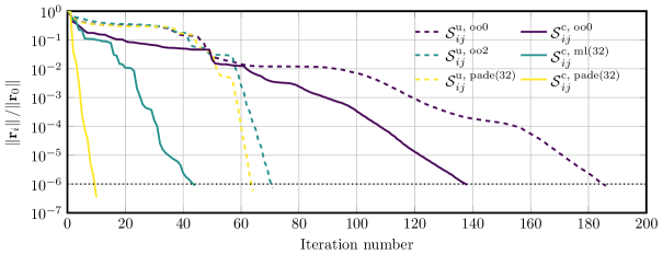
Figure 7: Convergence history of the GMRES solver – rectangular cavity with $D=2$ subdomains.

As the closed form solution $p_{\text{CF}}$ of this canonical problem is known, i.e.

$$p_{\text{CF}}=\sum_{m=1}^{K}\frac{\sin\left[k_{x}(m)(\ell-x)\right]}{\sin\left[k_{x}(m)\ell\right]}\sin\left[k_{y}(m)\right]$$ (47)

with

$$k_{y}(m)=m\frac{\pi}{h}\quad\text{and}\quad k_{x}(m)=\sqrt{k^{2}-k_{y}^{2}(m)},$$ (48)

let us determine the accuracy of the above simulations by computing the relative $L_{2}$ error $\operatorname{\mathcal{E}}$ between the FE solution $p_{\text{FE}}$ and $p_{\text{CF}}$:

$$\operatorname{\mathcal{E}}=\sqrt{\frac{\displaystyle\int_{\Omega}\mathinner{\!\left\lvert p_{\text{CF}}-p_{\text{FE}}\right\rvert}^{2}\mathrm{d}\Omega}{\displaystyle\int_{\Omega}\mathinner{\!\left\lvert p_{\text{CF}}\right\rvert}^{2}\mathrm{d}\Omega}},$$ (49)

where the above integrals are evaluated using a quadrature rule with twice the amount of integration points than the number used for the FE computations. The $L_{2}$ errors associated with the different OS schemes of Figure 7 are gathered in Table 2 together with the error associated with the MUMPS direct solver. These data show clearly that all transmission conditions and the direct solver lead to errors of the same order of magnitude.

$\operatorname{\mathcal{S}}_{ij}^{\text{u, oo0}}$	$\operatorname{\mathcal{S}}_{ij}^{\text{u, oo2}}$	$\operatorname{\mathcal{S}}_{ij}^{\text{u, pade($32$)}}$	$\operatorname{\mathcal{S}}_{ij}^{\text{c, oo0}}$	$\operatorname{\mathcal{S}}_{ij}^{\text{c, ml($32$)}}$	$\operatorname{\mathcal{S}}_{ij}^{\text{c, pade($32$)}}$	MUMPS
$1.76\times{}10^{-4}$	$1.76\times{}10^{-4}$	$1.78\times{}10^{-4}$	$1.77\times{}10^{-4}$	$1.76\times{}10^{-4}$	$1.77\times{}10^{-4}$	$1.78\times{}10^{-4}$

Table 2: Relative $L_{2}$ errors $\operatorname{\mathcal{E}}$ – rectangular cavity with $D=2$ subdomains.

Let us now focus on the wall-clock time required to complete the above computations, as reported in Table 3. In order to analyze these values, let us stress that they heavily depend on the actual software implementation of the FE and OS tools. Nonetheless, some general remarks can be drawn.

1. The OO0^u, OO2^u and OO0^c operators are the computationally cheapest to apply, as they do not involve auxiliary unknowns.

2. The ML^c and PADE^c operators are computationally more expensive than PADE^u, since they require two sets of auxiliary unknowns as they are not symmetric, i.e. $\operatorname{\mathcal{S}}_{ij}^{\text{c, ml($N$)/pade($N$)}}\neq\operatorname{\mathcal{S}}_{ji}^{\text{c, ml($N$)/pade($N$)}}$.

3. The regularization procedure involving PADE^u further increases the computational cost, as additional auxiliary unknowns are introduced.

In the current software implementation, the subproblems are solved with the direct solver MUMPS and the resulting LU factorization is reused in the subsequent OS iterations. Therefore, the first iteration is more time consuming than the other ones and the data in Table 3 are thus split in different subquantities. By defining $T_{i}$ as the share of the total wall clock time $T_{\text{tot}}$ dedicated to the $i$^th iteration, i.e. $T_{\text{tot}}=\sum_{i=1}^{I}T_{i}$ with $I$ the total number of GMRES iterations required for convergence, we report in Table 3 the following values: $T_{\text{tot}}$, $T_{1}$, $\overline{T_{2,I}}$, where $\overline{T_{i,j}}$ is the mean value of the sequence $[T_{i},\dots,T_{I}]$, and $I$.

Quantity of interest	$\operatorname{\mathcal{S}}_{ij}^{\text{u, oo0}}$	$\operatorname{\mathcal{S}}_{ij}^{\text{u, oo2}}$	$\operatorname{\mathcal{S}}_{ij}^{\text{u, pade($32$)}}$	$\operatorname{\mathcal{S}}_{ij}^{\text{c, oo0}}$	$\operatorname{\mathcal{S}}_{ij}^{\text{c, ml($32$)}}$	$\operatorname{\mathcal{S}}_{ij}^{\text{c, pade($32$)}}$	Unit
$T_{\text{tot}}$	113	48	48	90	41	17	s
$T_{1}$	9.52	9.37	10.14	9.44	10.90	10.99	s
$\overline{T_{2,I}}$	0.56	0.56	0.60	0.58	0.69	0.69	s
$I$	186	71	64	138	44	10	-

Table 3: Wall-clock times – rectangular cavity with $D=2$ subdomains ($T_{i}$ is the share of the total wall-clock time, in seconds, taken by the $i$^th iteration, $I$ is the total number of GMRES iterations and $\overline{T_{i,j}}$ is the mean value of the sequence $[T_{i},\dots,T_{j}]$).

From the data gathered in Table 3, it is clear that $\operatorname{\mathcal{S}}_{ij}^{\text{c, pade($32$)}}$ leads to both the minimal amount of iterations and the fastest computation with respect to the wall clock time. Nonetheless, it is evident that the cost of $T_{1}$ and $\overline{T_{2,I}}$ is higher for $\operatorname{\mathcal{S}}_{ij}^{\text{c, pade($32$)}}$ and $\operatorname{\mathcal{S}}_{ij}^{\text{c, ml($32$)}}$ than for the other transmission operators, in accordance with the remarks drawn above. The novel operators will therefore lead to the fastest computations only when the reduction of the iteration count is sufficiently high, when compared with the transmission conditions optimized for unbounded problems (see related discussion in sections 9).

7.2 Spectrum of the iteration operators

In this section, let us briefly discuss the spectra of the discretized iteration operator $\mathcal{F}=\operatorname{\mathcal{I}}-\operatorname{\mathcal{A}}$, which we will refer to as $F$ from now on. As the explicit construction of $F$ is computationally heavy, only the case of $D=2$ subdomains is considered here. It is also important to stress that $F$ is not a normal matrix, as it can be directly seen from the formal expression of $F$ in the case of two subdomains (see [14, section 2.3.1] for instance). As a consequence, the behavior of the GMRES cannot be predicted from the spectrum $\operatorname{Eig}(F)$ of the system matrix $F$ [31]. Nonetheless, eigenvalues that are clustered near $1$ are a good indicator that those modes are well captured by a given transmission operator.

The spectra in Figure 8 are associated with the novel transmission operators optimized for the rectangular cavity. Let us stress that the eigenvalues are all real in the present example. However, the spectrum of $F$ can be complex, even when its coefficients are all real, as it is non-normal. With the $\operatorname{\mathcal{S}}_{ij}^{\text{c, ml($N$)}}$ and $\operatorname{\mathcal{S}}_{ij}^{\text{c, pade($N$)}}$ operators, we can directly see from the displayed data that for sufficiently large values of $N$ (i.e. here $N=64$) the spectrum of $F$ lies within the unit circle centered around $1$. This shows that those operators are good approximations of the $\operatorname{DtN}$ map of the rectangular cavity. On the other hand, only a few eigenvalues are located around $1$ with the $\operatorname{\mathcal{S}}_{ij}^{\text{c, oo0}}$ operator.

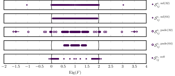
Figure 8: Spectrum of the discrete iteration operator $F$ for the different transmission operators optimized for rectangular cavities – rectangular cavity with $D=2$ subdomains (note that i) the spectrum is real, ii) the black arcs crossing $0$ and $2$ represent a portion of the unit circle centered around $1$ and iii) the arrows indicate that a few eigenvalues are outside the range shown here).

When using a transmission operator optimized for unbounded problem in a cavity setting, the spectra in Figure 9 are obtained. As expected from the analysis of section 6, the $\operatorname{\mathcal{S}}_{ij}^{\text{u, oo0}}$ operator leads to eigenvalues lying on the unit circle $\mathcal{C}$ centered around $1$. In addition, the behavior of the PADE^u operators has been well anticipated by our previous discussions as well. It is indeed clear that the eigenvalues of $F$ fall into two categories:

1. those associated with evanescent modes, which form a cluster similar to the PADE^c one and

2. those associated with non-evanescent modes, that lie on $\mathcal{C}$.

To conclude this subsection, let us also stress that despite a clustering significantly better for the PADE^u operators than for OO2^u, both operators exhibit rather similar GMRES convergence curves, as shown in Figure 7. This shows the difficulty in predicting the convergence of GMRES from $\operatorname{Eig}(F)$, since $F$ is non-normal.

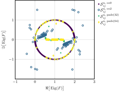
Figure 9: Spectrum of the discrete iteration operator $F$ for the different transmission operators optimized for unbounded problems – rectangular cavity with $D=2$ subdomains.

7.3 Regularized and mixed transmission conditions

As discussed in sections 4.5 and 4.6, a regularization term or a mixed transmission condition can be used to prevent the convergence radius from becoming very large (or, in the worst case, ill-defined). The performance of those transmission conditions is shown in Figures 10(a) and 10(b) for $\operatorname{\mathcal{S}}_{ij}^{\text{c, oo0, r($\chi$)}}$ and $\operatorname{\mathcal{S}}_{ij}^{\text{m($\varepsilon,M$), oo0}}$ respectively with $D=8$ subdomains. It is clear from the figures that regularizing the OO0^c operator by adding an imaginary part comes at the cost of an increased number of iterations. On the other hand, mixing OO0^c with PADE^u leads to an improvement in terms of iteration count. Nonetheless, in all cases, the regularized operators do not lead to any improvement with respect to the PADE^u conditions. Let us also note that the regularized operators tend to the original OO0^c as $\chi$ becomes small (resp. $\varepsilon$ becomes large).

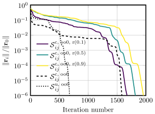
(a) Regularization with a constant imaginary part.

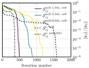
(b) Regularization with a mixed operator.

Figure 10: Regularized and mixed OO0^c – rectangular cavity with $D=8$ subdomains.

A similar numerical experiment can also be carried out for the regularization of the ML^c condition. From the GMRES convergence histories depicted in Figure 11, it can be noticed that while the performance of ML^c remains better than PADE^u, the regularization increases the number of iterations required to reach convergence. Nonetheless, this increase declines as the regularization becomes lighter, i.e. when $\chi$ (resp. $\varepsilon$) becomes small (resp. large).

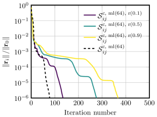
(a) Regularization with a constant imaginary part.

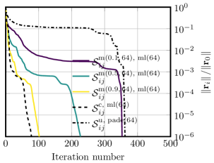
(b) Regularization with a mixed operator.

Figure 11: Regularized and mixed ML^c – rectangular cavity with $D=8$ subdomains.

An analogous numerical experiment is performed once more for the regularization of the PADE^c condition. This last scenario shows a behavior similar to ML^c, as it can be directly observed in Figure 12.

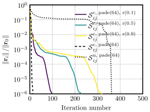
(a) Regularization with a constant imaginary part.

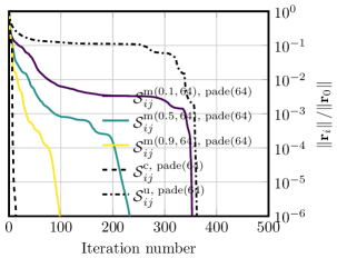
(b) Regularization with a mixed operator.

Figure 12: Regularized and mixed PADE^c – rectangular cavity with $D=8$ subdomains.

7.4 Impact of the number of auxiliary unknowns

Let us now investigate the impact of the number of auxiliary unknowns $N$ appearing in $\operatorname{\mathcal{S}}_{ij}^{\text{u, pade($N$)}}$, $\operatorname{\mathcal{S}}_{ij}^{\text{c, ml($N$)}}$ and $\operatorname{\mathcal{S}}_{ij}^{\text{c, pade($N$)}}$ on the number of iteration of the GMRES solver. The numerical results are shown in Figure 13 for a numerical experiment involving $D=8$ subdomains of equal size. It is clear from the data that every operator converges with values of $N$ as low as $N=1$. Nonetheless, for the novel operators to outperform the convergence of the PADE^u operator, a minimum value of $N_{\text{min}}^{\text{data}}=8$ is required in this example. It is also evident in this example that $\operatorname{\mathcal{S}}_{ij}^{\text{c, pade($N$)}}$ always performs better than $\operatorname{\mathcal{S}}_{ij}^{\text{c, ml($N$)}}$ for a fixed value of $N$. Last but not least, it is evident from Figure 13 that $N$ has only a mild effect on the performance of $\operatorname{\mathcal{S}}_{ij}^{\text{u, pade($N$)}}$.

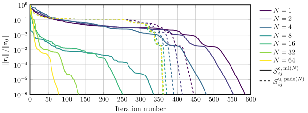
(a) Mittag-Leffler expansion.

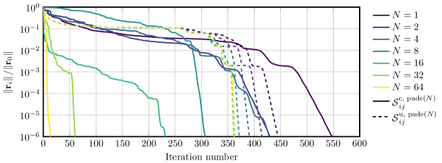
(b) Padé expansion.

Figure 13: Convergence history of the GMRES solver for different number of auxiliary unknown in the case of $D=8$ subdomains.

It is also interesting to compare the value of $N_{\text{min}}^{\text{data}}$ found experimentally and the value predicted with the pole criterion discussed in section 4.7. In this numerical experiment, the largest $\ell_{ij}$ is $\ell_{ij}^{\text{max}}=\frac{7}{8}\ell$ and thus $N_{\text{min}}^{\text{pole}}=44$ according to the pole criterion (33). Consequently, $N_{\text{min}}^{\text{pole}}$ is a pessimistic estimation in this case, since $N_{\text{min}}^{\text{data}}<N_{\text{min}}^{\text{pole}}$.

7.5 Increase in the number of rectangular subdomains

In this section we focus on the impact of the number of subdomains $D$ onto the GMRES iteration count, as shown in Figure 14. From this plot, is clear that $\operatorname{\mathcal{S}}_{ij}^{\text{c, pade($64$)}}$ leads to an increase in the number of GMRES iterations with the optimal slope of $2D$, at least for the considered range of $D$. Let us mention also that the unbounded transmission operators exhibit a significantly larger slope, motivating thus the use of transmission conditions specifically devised for cavity problems. Furthermore let us note that $\operatorname{\mathcal{S}}_{ij}^{\text{u, pade($64$)}}$ and $\operatorname{\mathcal{S}}_{ij}^{\text{u, oo2}}$ present the same slope, as they are both excellent localization of the unbounded $\operatorname{DtN}$ map. In addition, while the $\operatorname{\mathcal{S}}_{ij}^{\text{c, ml($64$)}}$ operator shows a suboptimal scaling with respect to $D$, it outperforms $\operatorname{\mathcal{S}}_{ij}^{\text{u, pade($64$)}}$ and $\operatorname{\mathcal{S}}_{ij}^{\text{u, oo2}}$. Last but not least, it is evident from Figure 14 that the scaling behavior of $\operatorname{\mathcal{S}}_{ij}^{\text{c, oo0}}$ is the worst of all.

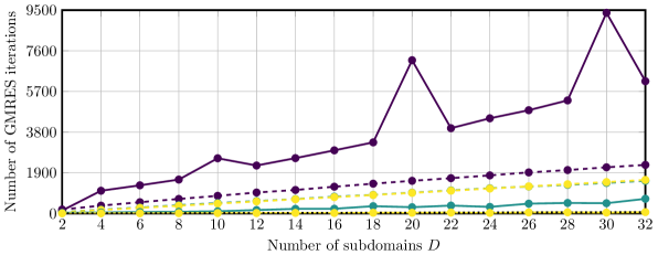
(a) Zoom level 0: focus on OO0^c.

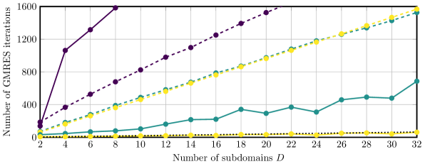
(b) Zoom level 1: focus on OO0^u, OO2^u, PADE^u and ML^c.

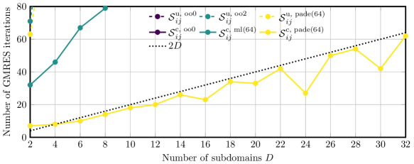
(c) Zoom level 2: focus on PADE^c

Figure 14: Number of GMRES iterations as a function of the number of subdomains (raw numbers available in Table 4).

7.6 Impact of the length-to-wavelength ratio

The dependence of the GMRES iteration count on the wavenumber is a major performance indicator of an OS scheme, and a numerical experiment analyzing this is therefore carried out. In this investigation the values of $\ell/\lambda_{w}$ are chosen close to an integer value, which corresponds to a cavity driven at a frequency close to one of its resonance frequencies. The computational domain is partitioned into $D=8$ subdomains and the cavity is excited with double the amount of non-evanescent modes (this number depending on $\ell/\lambda_{w}$). It is clear from the data shown in Figure 15 that the iteration count increases rapidly with $\ell/\lambda_{w}$ with the unbounded transmission operators. This growth in the iteration count is, nonetheless, not as fast as for $\operatorname{\mathcal{S}}_{ij}^{\text{c, oo0}}$. On the other hand, the situation is significantly improved with $\operatorname{\mathcal{S}}_{ij}^{\text{c, ml($N$)}}$ and the iteration count becomes almost independent from $\ell/\lambda_{w}$ with $\operatorname{\mathcal{S}}_{ij}^{\text{c, pade($N$)}}$, at least in the considered $\ell/\lambda_{w}$ range. Let us also note that similar results are obtained when $\ell/\lambda_{w}$ is selected away from a resonance.

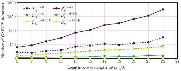
(a) Zoom level 0: focus on OO0^c.

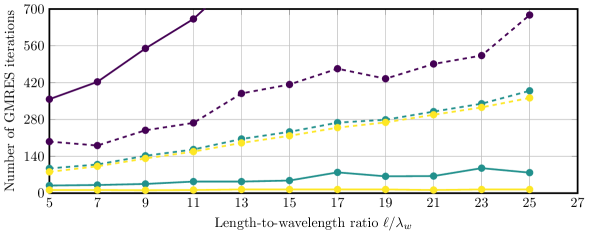
(b) Zoom level 1: focus on OO0^u, OO2^u and PADE^u.

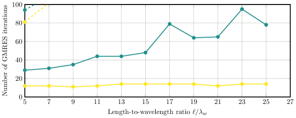
(c) Zoom level 2: focus on ML^c and PADE^c.

Figure 15: Number of GMRES iterations as a function of the length-to-wavelength ratio for a cavity with $D=8$ subdomains (raw numbers available in Table 5).

7.7 Discussion

From the data gathered in the previous numerical examples, it is obvious that the $\operatorname{\mathcal{S}}_{ij}^{\text{c, oo0}}$ operator leads to a poor scaling when $D>2$. For this reason, this operator and its regularized variants are not further considered in this work.

It is also clear that for rectangular cavities the $\operatorname{\mathcal{S}}_{ij}^{\text{c, pade($N$)}}$ and $\operatorname{\mathcal{S}}_{ij}^{\text{c, ml($N$)}}$ operators converge with significantly less iterations than their unbounded alternatives, i.e. $\operatorname{\mathcal{S}}_{ij}^{\text{u, pade($N$)}}$, $\operatorname{\mathcal{S}}_{ij}^{\text{u, oo2}}$ and $\operatorname{\mathcal{S}}_{ij}^{\text{u, oo0}}$, and exhibit a better scaling with increasing values of $D$. Nonetheless, let us recall that the novel operators i) are associated with a higher computational cost and ii) are more sensitive to numerical errors in finite precision arithmetic. This latter point motivates the use of the modified version of the Gram-Schmidt algorithm in the GMRES orthogonalization step.

It is also worth noticing that the unbounded operator $\operatorname{\mathcal{S}}_{ij}^{\text{u, pade($N$)}}$ and $\operatorname{\mathcal{S}}_{ij}^{\text{u, oo2}}$ lead to very similar convergence profiles, which is not surprising as they both are excellent approximations of the unbounded $\operatorname{DtN}$ map. For this reason, only the $\operatorname{\mathcal{S}}_{ij}^{\text{u, pade($N$)}}$ operator will be further considered.

Another interesting result concerns the impact of a change of the wavenumber on the convergence profile of the above transmission operators. For the considered range of length-to-wavelength ratios $\ell/\lambda_{w}$, we observed that the $\operatorname{\mathcal{S}}_{ij}^{\text{c, pade($N$)}}$ behaves quasi-independently from $\ell/\lambda_{w}$, while the other operators exhibit a (quasi) linear increase of the iteration count with $\ell/\lambda_{w}$. Nonetheless, the slope of this increase remains small for $\operatorname{\mathcal{S}}_{ij}^{\text{c, ml($N$)}}$ when compared with $\operatorname{\mathcal{S}}_{ij}^{\text{u, oo0}}$, $\operatorname{\mathcal{S}}_{ij}^{\text{u, oo2}}$ and $\operatorname{\mathcal{S}}_{ij}^{\text{u, pade($N$)}}$.

Let us finally note that similar experiments were carried out on three-dimensional rectangular parallelepipedic cavities with a square cross-section of $h\times{}h$ and a length of $\ell$. Results analogous to the above two-dimensional test cases were obtained.

8 Sensitivity to geometrical parameters

The previous section considered only one geometry (a rectangular cavity and its three-dimensional equivalent), which refers to the specific configuration used to devise the transmission operators discusses in section 4. Nonetheless, relevant simulations involve computational domains that differ from this original setting. We therefore discuss in this section two geometries deviating from the canonical one.

8.1 Trapezoidal geometry – modified Gram-Schmidt variant

For this first numerical experiment, let us consider an isosceles trapezoid whose base is characterized with a parameter $\delta$, as the one depicted in Figure 16. This computational domain is partitioned into $D=16$ subdomains and, as with the previous rectangular cavity, the aspect ratio $\ell/h$ equals $2$ and the length-to-wavelength ratio $\ell/\lambda_{w}$ is approximately $25.001$.

Figure 16: Isosceles trapezoid considered in the numerical experiment.

The number of GMRES iterations associated with various operators are shown in Figure 17 for different values of $\delta$. It is clear from the depicted results that the novel rational operators outperform, in all considered cases, the $\operatorname{\mathcal{S}}_{ij}^{\text{u, pade($64$)}}$ one in terms of iteration count, even when no regularization is applied. Additionally, the $\operatorname{\mathcal{S}}_{ij}^{\text{c, pade($64$)}}$ is systematically the best choice and its regularization always leads to a slight increase in the iteration count. In the case of the ML^c variant, regularization slightly improves the convergence for the highest value of $\delta$. Furthermore, there is an evident trend in the displayed data showing an increase in the iteration count as $\delta$ increases. However, as this increase also affects $\operatorname{\mathcal{S}}_{ij}^{\text{u, pade($64$)}}$, it is hard to predict if and when this operator will overtake the novel ones, at least in terms of iteration count.

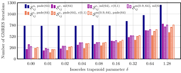
Figure 17: Iteration count of the GMRES solver when used on a trapezoidal geometry partitioned into $D=16$ subdomains (raw numbers available in Table 6).

8.2 Trapezoidal geometry – classical Gram-Schmidt variant

In the introduction of section 7, we mentioned that using the modified version of the Gram-Schmidt (GS) algorithm is critical for the convergence, as the novel transmission conditions involve operators oscillating rapidly in a wide range. In order to assess the importance of this choice, we carry out once more the previous numerical experiments using the classical version of the GS orthogonalization procedure [27].

As it would be impractical to show the data for all possible combinations, only the case with PADE^u and PADE^c (with and without regularization) at $\delta=32$ is shown in Figure 18, as it contains the different behavior we want to highlight. First of all, it is clear from the displayed data that the modified GS does not impact the behavior of the PADE^u operator. In addition, it is also evident that it prevents stagnation and improves the overall convergence with PADE^c.

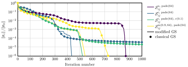
Figure 18: Convergence history of the GMRES solver with the classical and the modified Gram-Schmidt (GS) procedures, when used on a trapezoidal geometry partitioned into $D=16$ subdomains.

Regarding the other combinations that are not shown in Figure 18, we observed that: i) a relative residual $\mathinner{\!\left\lVert\mathbf{r}_{i}\right\rVert}/\mathinner{\!\left\lVert\mathbf{r}_{0}\right\rVert}$ smaller than $10^{-6}$ is not always reached when using the classical Gram-Schmidt procedure, ii) this relative residual is always reached with the modified GS, iii) the convergence history of the PADE^u operator is identical for both GS variants and iv) the modified GS is never worse than the classical GS.

8.3 Rectangular cavity involving obstacles – impact of the number of obstacles

Let us now study again a rectangular cavity, but let us introduce $O$ circular obstacles in the domain. As in the previous case, we have $\ell/h=2$ and $\ell/\lambda_{w}\approx 25.001$. Furthermore, we assume that the obstacles exhibit a hard-wall behavior and that each subdomain includes at most one obstacle located in its center. A sketch of a possible configuration is shown in Figure 19, with $O=3$ obstacles and $D=3$ subdomains.

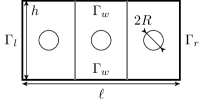
Figure 19: Rectangular cavity involving $O=3$ obstacles and $D=3$ subdomains.

We carry out a first numerical experiment consisting in determining the number of iterations as a function of the number of obstacles $O$. The obstacles are introduced by starting from the middle of the cavity and then by adding them equally on both sides. We consider a domain partitioning involving $D=17$ subdomains, leading thus to a maximum number of obstacles of $O=17$, and a radius of $R=0.5\lambda_{w}$ for the obstacles. The results of this experiment are gathered in Figure 20. First of all, it is worth mentioning that when $O=1$, the transmission condition $\operatorname{\mathcal{S}}_{ij}^{\text{c, pade($64$)}}$ exhibits an excellent performance compared with the other operators. The operator $\operatorname{\mathcal{S}}_{ij}^{\text{c, ml($64$)}}$ also shows a good performance, in comparison with the unbounded Padé operator. This lead with respect to $\operatorname{\mathcal{S}}_{ij}^{\text{u, pade($64$)}}$ decreases however as $O$ increases. Nonetheless, in all considered cases, the novel conditions are associated with a lower iteration count than $\operatorname{\mathcal{S}}_{ij}^{\text{u, pade($64$)}}$, although this gain is modest for higher values of $O$. In this regard, the ML^c condition performs slightly better for higher values of $O$, while PADE^c is better for the lower values. Concerning the regularized variants, they lead to higher iteration counts than their unregularized variants, apart from the two highest values of $O$, where regularization is slightly beneficial to the PADE^c operator. Before concluding this subsection, let us stress that we used different values for the number of terms $M$ and $N$ in the mixed operators $\operatorname{\mathcal{S}}_{ij}^{\text{m($\varepsilon,M$), ml($N$)/pade($N$)}}$.

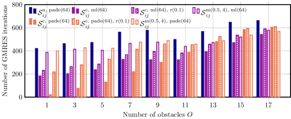
Figure 20: Iteration count of the GMRES solver when used on a rectangular cavity involving $O$ obstacles of radius $R=0.5\lambda_{w}$ and $D=17$ subdomains (raw numbers available in Table 7).

8.4 Rectangular cavity involving obstacles – impact of the size of the obstacles

In the previous subsection we assumed a rather large radius for the obstacles compared with the wavelength and focused only on the number of obstacles. Let us now reverse the study and let us determine the impact of the obstacle size on the performance of the transmission operators. To this end, let us again consider a rectangular cavity with $D=17$ subdomains and $O=7$ obstacles of radius $R$ and let us gather in Figure 21 the number of iterations required to solve this problem as $R$ varies. Concerning the novel conditions, the displayed data show a clear trend pointing toward an increase of the iteration count as $R$ increases. While this increase is systematic for $\operatorname{\mathcal{S}}_{ij}^{\text{c, pade($64$)}}$, a plateau can be seen with $\operatorname{\mathcal{S}}_{ij}^{\text{c, ml($64$)}}$ for the three intermediate values of $R$. As in the previous numerical experiment, let us note i) that the novel conditions outperform $\operatorname{\mathcal{S}}_{ij}^{\text{u, pade($64$)}}$ in all cases and ii) that regularization leads to an increased iteration count.

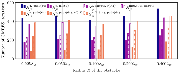
Figure 21: Iteration count of the GMRES solver when used on a rectangular cavity involving $O=7$ obstacles and $D=17$ subdomains (raw numbers available in Table 8).

8.5 Discussion

The above numerical experiments clearly show that, while the performance of the novel $\operatorname{\mathcal{S}}_{ij}^{\text{c, ml($N$)}}$ and $\operatorname{\mathcal{S}}_{ij}^{\text{c, pade($N$)}}$ operators deteriorates as the geometry of the problem deviates from the reference rectangular case, this deterioration does not exhibit sudden jumps as the geometry is modified. In addition, the sensitivity of the novel operators with respect to numerical errors stemming from finite precision arithmetic is also clearly shown by our data, motivating the use of the modified Gram-Schmidt algorithm in the orthogonalization step of GMRES.

When compared to the PADE^u operator, PADE^c and ML^c clearly outperform the former for small deviations. On the other hand, in all considered cases, the reduction of the iteration count brought by PADE^c and ML^c can become modest (with respect to PADE^u) for large deviations. Nonetheless, we did not encounter situations where PADE^u leads to clear gain, at least in terms of iteration count and within the scope of the numerical experiment considered in this work. This suggests a rather robust behavior of PADE^c and ML^c.

9 Engineering test case: acoustic noise in a three-dimensional model of the helium vessel of a beamline cryostat

Going back to the experiment with a rectangular cavity filled with obstacles, it has been shown that the PADE^c operator shows a very fast convergence when the cavity exhibits only one obstacle, as shown in Figure 20. Additionally, the same behavior is observed for other configurations exhibiting a unique circular obstacle. A such characteristic can be very well suited when, for instance, simulating the acoustic noise in the helium vessel of a beamline cryostat, which basically consists of a rectangular cavity interrupted by a circular obstacle (e.g. see the cryostat discussed in [32]). Such acoustic noise analyses can become critical, for instance, when designing a cryogenic current comparator (CCC) with a large bore [33]. A CCC is one of the most sensitive instrument for measuring very low electric currents with high accuracy and can be used e.g. in particle accelerators for the non-destructive monitoring of slowly extracted charged particle beams (current intensities below $1\mu{}A$) [33].

Within this context, let us compare the behavior of the different transmission operators on a helium vessel model consisting in a rectangular parallelepipedic cavity interrupted with a cylindrical obstacle and partitioned into $D=8$ subdomains. The model is excited with its first spatial mode, the length-to-wavelength ratio is chosen as $\ell/\lambda_{w}\simeq 12.5004$ and the cross-section is $h\times{}h$ with $h=\ell/2$. This numerical experiment leads to the convergence history displayed in Figure 22 for each transmission operator. It is clear from these data that the $\operatorname{\mathcal{S}}_{ij}^{\text{c, pade($24$)}}$ leads to the quickest convergence and requires only $50$ iterations to converge. Compared with the $93$ iterations required by $\operatorname{\mathcal{S}}_{ij}^{\text{u, pade($24$)}}$, a reduction of the iteration count of approximately $46\%$ is achieved. Figure 22 shows as well the impact of a light regularization of the PADE^c and ML^c operators. As expected, no performance gain is obtained, as the unregularized counterparts already converge well. For illustration purposes, the computed field map is available in Figure 23.

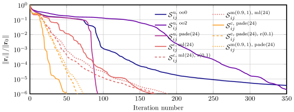
Figure 22: Convergence history of the GMRES solver – helium vessel of a beamline cryostat with $D=8$ subdomains.

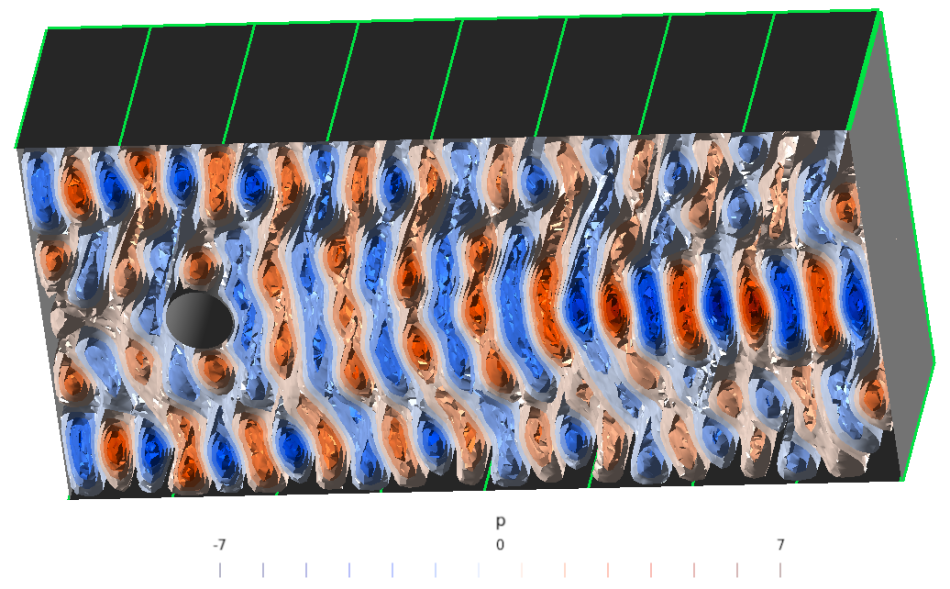
Figure 23: Field map of the simulated helium vessel (view rotated by $90^{\circ}$, subdomains are highlighted with green lines).

The above analysis would not be complete without considering the wall clock time. As already discussed in section 7, the novel transmission operators optimized for cavity problems are associated with an increased computational cost, when compared with their unbounded counterparts. As a result, in the context of the considered acoustic study, the OO0^u and OO2^u operators lead to the fastest computations (i.e. approximately $3.5$ and $3$ hours respectively), despite their rather slow convergence. In comparison with OO2^u, the rational operators see their wall clock time increased by a factor of i) $2$for PADE^u, ii) $2.7$for ML^c and iii) $2.5$for PADE^c.

Before concluding this section, it is important to stress that the current implementation does not treat the auxiliary unknowns in the most efficient way. For instance, it assembles all auxiliary unknowns into a single large system. However, the extra unknowns stemming from the asymmetric nature of $\operatorname{\mathcal{S}}_{ij}^{\text{c, ml($N$)/pade($N$)}}$ could be pulled out into smaller auxiliary systems, which could improve the overall computational time. Let us also mention that the OS iterative scheme can also be altered, such that all auxiliary unknowns are decoupled from the subproblems, as proposed in [34]. Such improvements are left for a future work.

10 Conclusion and final remarks

In this work we presented new transmission operators for the Schwarz method optimized for time-harmonic Helmholtz problems in a rectangular cavity. Those operators rely on different localizations of the Dirichlet-to-Neumann map of this reference geometry. Three different strategies were considered for devising local approximations of the Fourier symbol of the $\operatorname{DtN}$, namely: i) a zeroth-order Taylor approximation, ii) a truncated Mittag-Leffler partial fraction expansion and iii) a Padé approximant. As these operators do not necessarily lead to a well defined scheme, two regularization procedures where proposed to correct this problem. Let us however mention that, when combined with the modified variant of the Gram-Schmidt procedure in the orthogonalization step of GMRES (without restart), the proposed operators led to convergent iterative schemes in all the numerical experiments considered in this work, even in the unregularized case.

The new operators optimized for cavity problems were also compared with operators optimized for unbounded geometries, yet applied to cavities. In the case of the reference rectangular geometry, the gain in the iteration count brought by the novel rational operators is clear when compared with the unbounded ones. On the other hand, when considering geometries deviating from the canonical one, this iteration count gain decreases. Nonetheless, even if the gain can be modest for large deviations, the new rational operators always led to a lower iteration count (than their unbounded counterparts) in the considered numerical experiments. Of course, this does not guarantee that the novel rational operators will always perform better, but this suggests that they are sufficiently robust with respect to geometrical changes. The computational cost of the different transmission operators was also briefly discussed, as well as some possible improvements for reducing it.

To conclude this paper, let us draw some final remarks regarding the selection of an operator. While a detailed analysis is out of the scope of this work, some general trends can be extracted from this study. First of all, when considering the wall-clock time, as the computational cost of the novel rational operators is high, a simple OO0^u operator might be a good default choice. Nonetheless, as already mentioned, alterations of the Schwarz scheme could improve this aspect. On the other hand, when focusing only on the iteration count, the PADE^c operator (with a small regularization) can be recommended as a first guess. Indeed, since evanescent modes in cavities and unbounded problems converge quickly to each other, both Padé based approximations should behave similarly for these modes if $N$ is sufficiently large. Let us note that this is coherent with the spectra discussed in section 7.2. Thus, the difference between PADE^c and PADE^u lies mainly in the non-evanescent part, for which the PADE^u is clearly a poor approximation. Therefore, in the worst case scenario, it is legitimate to expect that both PADE^c and PADE^u will behave similarly, at least with a GMRES without restart, as shown in our numerical experiments. Let us note that this expectation still needs to be investigated more formally, which is left for a future work.

Declaration of competing interest

The authors declare that they have no known competing financial interests or personal relationships that could have appeared to influence the work reported in this paper.

Appendix A Calculation of the convergence radius – non-overlapping case

In this appendix, let us briefly discuss the main steps of the calculation leading to the Fourier symbol of the Dirichlet-to-Neumann map shown in equation (9). To this end, we start with case $s^{2}\neq k^{2}$, and write the solutions of (6a) and (6d), together with the boundary conditions (6c) and (6f) and the definition (7). Formally, we obtain:

$$[left=\empheqlbrace]\widehat{p}_{0}^{n+1}(x,s) =P_{0}^{n+1}(s)\,\frac{\sinh\left[+\alpha\left(\frac{\ell}{2}+x\right)\right]}{\sinh\left[+\alpha\left(\frac{\ell}{2}+\gamma\right)\right]} \forall x\in\left[-\frac{\ell}{2},\gamma\right],\forall s\in\mathbb{S},s^{2}\neq{}k^{2},$$ (50a)

$$\widehat{p}_{1}^{n+1}(x,s) =P_{1}^{n+1}(s)\,\frac{\sinh\left[-\alpha\left(\frac{\ell}{2}-x\right)\right]}{\sinh\left[-\alpha\left(\frac{\ell}{2}-\gamma\right)\right]} \forall x\in\left[\gamma,+\frac{\ell}{2}\right],\ \forall s\in\mathbb{S},s^{2}\neq{}k^{2},$$ (50b)

where

$$[left={\alpha(s)=\empheqlbrace}] -\jmath\sqrt{k^{2}-s^{2}} \text{if}~{}s^{2}<k^{2},$$ (51a)

$$0 \text{if}~{}s^{2}=k^{2},$$ (51b)

$$\sqrt{s^{2}-k^{2}} \text{if}~{}s^{2}>k^{2}.$$ (51c)

This solution can then be derived with respect to $x$ and the result evaluated at the interface between the subdomains, i.e. at $x=\gamma(t)=t\ell-\ell/2$ with $t\in[0,1]$ as discussed in section 2. We thus have that

$$[left=\empheqlbrace]\left.\frac{\partial\widehat{p}_{0}^{n+1}}{\partial x}(x,s)\right|_{x=\gamma(t)} =\alpha\,P_{0}^{n+1}\,\coth\mathopen{}\left[+\alpha{}t\ell\mathclose{}\right] \forall s\in\mathbb{S},s^{2}\neq{}k^{2},$$ (52a)

$$\left.\frac{\partial\widehat{p}_{1}^{n+1}}{\partial x}(x,s)\right|_{x=\gamma(t)} =\alpha\,P_{1}^{n+1}\,\coth\mathopen{}\left[-\alpha(1-t)\ell\mathclose{}\right] \forall s\in\mathbb{S},s^{2}\neq{}k^{2}.$$ (52b)

The convergence radius $\rho(s)$ is then obtained by simplifying the transmission conditions (6b) and (6e) with the above expressions. In particular, we can write

$$[left=\empheqlbrace]P_{0}^{n+1} =P_{0}^{n-1}\frac{\lambda_{10}-\alpha\coth\left[\alpha{}t\ell\right]}{\lambda_{10}+\alpha\coth\left[\alpha{}(1-t)\ell\right]}\frac{\lambda_{01}-\alpha\coth\left[\alpha{}(1-t)\ell\right]}{\lambda_{01}+\alpha\coth\left[\alpha{}t\ell\right]}=P_{0}^{n-1}\rho^{2}(s),$$ (53a)

$$P_{1}^{n+1} =P_{1}^{n-1}\frac{\lambda_{01}-\alpha\coth\left[\alpha{}(1-t)\ell\right]}{\lambda_{01}+\alpha\coth\left[\alpha{}t\ell\right]}\frac{\lambda_{10}-\alpha\coth\left[\alpha{}t\ell\right]}{\lambda_{10}+\alpha\coth\left[\alpha{}(1-t)\ell\right]}=P_{1}^{n-1}\rho^{2}(s).$$ (53b)

Equation (9) is thus recovered, for the case $s^{2}\neq k^{2}$, by identifying the above terms and by exploiting the definition of $\alpha(s)$, $\ell_{01}$ and $\ell_{10}$, that is

$$[left=\empheqlbrace]\ell_{01} =t\ell,$$ (54a)

$$\ell_{10} =(1-t)\ell.$$ (54b)

Let us now treat the case $s^{2}=k^{2}$. In this case $\widehat{p}_{i}^{n+1}(x,s)$ writes

$$[left=\empheqlbrace]\widehat{p}_{0}^{n+1}(x,s) =P_{0}^{n+1}\frac{x+\ell/2}{\gamma+\ell/2} \forall x\in\left[-\frac{\ell}{2},\gamma\right],s^{2}=k^{2},$$ (55a)

$$\widehat{p}_{1}^{n+1}(x,s) =P_{1}^{n+1}\frac{x-\ell/2}{\gamma-\ell/2} \forall x\in\left[\gamma,+\frac{\ell}{2}\right],s^{2}=k^{2},$$ (55b)

and its derivative evaluated at $x=\gamma$ is simply:

$$[left=\empheqlbrace]\left.\frac{\partial\widehat{p}_{0}^{n+1}}{\partial x}(x,s)\right|_{x=\gamma(t)} =+P_{0}^{n+1}\frac{1}{t\ell} \forall s\in\mathbb{S},s^{2}=k^{2},$$ (56a)

$$\left.\frac{\partial\widehat{p}_{1}^{n+1}}{\partial x}(x,s)\right|_{x=\gamma(t)} =-P_{1}^{n+1}\frac{1}{(1-t)\ell} \forall s\in\mathbb{S},s^{2}=k^{2}.$$ (56b)

Therefore, the transmission conditions (6b) and (6e) become

$$[left=\empheqlbrace]P_{0}^{n+1} =P_{0}^{n-1}\frac{\lambda_{10}-\frac{1}{t\ell}}{\lambda_{10}+\frac{1}{(1-t)\ell}}\frac{\lambda_{01}-\frac{1}{(1-t)\ell}}{\lambda_{01}+\frac{1}{t\ell}}=P_{0}^{n-1}\rho^{2}(s=k),$$ (57a)

$$P_{1}^{n+1} =P_{1}^{n-1}\frac{\lambda_{01}-\frac{1}{(1-t)\ell}}{\lambda_{01}+\frac{1}{t\ell}}\frac{\lambda_{10}-\frac{1}{t\ell}}{\lambda_{10}+\frac{1}{(1-t)\ell}}=P_{1}^{n-1}\rho^{2}(s=k),$$ (57b)

revealing thus the convergence radius $\rho(s=k)$. Again, equation (9) is recovered, for the case $s^{2}=k^{2}$, by identifying the above terms and by exploiting the definition of $\ell_{01}$ and $\ell_{10}$.

Appendix B Calculation of the convergence radius – overlapping case

Let us now assume an overlap of $2\delta$ such that $\Sigma_{01}$ is located at $\gamma_{0}=\gamma+\delta$ and $\Sigma_{10}$ is located at $\gamma_{1}=\gamma-\delta$, where $\gamma(t)=t\ell-\ell/2$ with $t\in[0,1]$ as in the previous appendix. In the case $s^{2}\neq k^{2}$, the overlapping variant of (6a) and (6d), together with the boundary conditions (6c) and (6f) and the definition (7) admits the following solutions:

$$[left=\empheqlbrace]\widehat{p}_{0}^{n+1}(x,s) =P_{0}^{n+1}(s)\,\frac{\sinh\left[+\alpha\left(\frac{\ell}{2}+x\right)\right]}{\sinh\left[+\alpha\left(\frac{\ell}{2}+\gamma_{0}\right)\right]} \forall x\in\left[-\frac{\ell}{2},\gamma_{0}\right],\forall s\in\mathbb{S},s^{2}\neq{}k^{2},$$ (58a)

$$\widehat{p}_{1}^{n+1}(x,s) =P_{1}^{n+1}(s)\,\frac{\sinh\left[-\alpha\left(\frac{\ell}{2}-x\right)\right]}{\sinh\left[-\alpha\left(\frac{\ell}{2}-\gamma_{1}\right)\right]} \forall x\in\left[\gamma_{1},+\frac{\ell}{2}\right],\ \forall s\in\mathbb{S},s^{2}\neq{}k^{2},$$ (58b)

which is similar as for the non-overlapping case but with interfaces located at different positions, $x=\gamma_{0}$ and $x=\gamma_{1}$, instead of a unique one, $x=\gamma$. After evaluating those two solutions at $x=\gamma_{0}$ and $x=\gamma_{1}$, we obtain:

$$[left=\empheqlbrace]\widehat{p}_{0}^{n+1}(\gamma_{0},s) =P_{0}^{n+1}(s) \forall s\in\mathbb{S},s^{2}\neq{}k^{2},$$ (59a)

$$\widehat{p}_{1}^{n+1}(\gamma_{0},s) =P_{1}^{n+1}(s)\,\frac{\sinh\left[\alpha\left(\frac{\ell}{2}-\gamma-\delta\right)\right]}{\sinh\left[\alpha\left(\frac{\ell}{2}-\gamma+\delta\right)\right]} \forall s\in\mathbb{S},s^{2}\neq{}k^{2},$$ (59b)

and

$$[left=\empheqlbrace]\widehat{p}_{0}^{n+1}(\gamma_{1},s) =P_{0}^{n+1}(s)\frac{\sinh\left[\alpha\left(\frac{\ell}{2}+\gamma-\delta\right)\right]}{\sinh\left[\alpha\left(\frac{\ell}{2}+\gamma+\delta\right)\right]} \forall s\in\mathbb{S},s^{2}\neq{}k^{2},$$ (60a)

$$\widehat{p}_{1}^{n+1}(\gamma_{1},s) =P_{1}^{n+1}(s) \forall s\in\mathbb{S},s^{2}\neq{}k^{2}.$$ (60b)

Regarding the derivatives with respect to $x$ of $\widehat{p}_{0}^{n+1}(x,s)$ and $\widehat{p}_{0}^{n+1}(x,s)$ at $x=\gamma_{0}$ and $x=\gamma_{1}$, we have:

$$[left=\empheqlbrace]\left.\frac{\partial\widehat{p}_{0}^{n+1}}{\partial x}(x,s)\right|_{x=\gamma_{0}} =+\alpha\,P_{0}^{n+1}\,\frac{\cosh\left[\alpha\left(\frac{\ell}{2}+\gamma+\delta\right)\right]}{\sinh\left[\alpha\left(\frac{\ell}{2}+\gamma+\delta\right)\right]} \forall s\in\mathbb{S},s^{2}\neq{}k^{2},$$ (61a)

$$\left.\frac{\partial\widehat{p}_{1}^{n+1}}{\partial x}(x,s)\right|_{x=\gamma_{0}} =-\alpha\,P_{1}^{n+1}\,\frac{\cosh\left[\alpha\left(\frac{\ell}{2}-\gamma-\delta\right)\right]}{\sinh\left[\alpha\left(\frac{\ell}{2}-\gamma+\delta\right)\right]} \forall s\in\mathbb{S},s^{2}\neq{}k^{2},$$ (61b)

and

$$[left=\empheqlbrace]\left.\frac{\partial\widehat{p}_{0}^{n+1}}{\partial x}(x,s)\right|_{x=\gamma_{1}} =+\alpha\,P_{0}^{n+1}\,\frac{\cosh\left[\alpha\left(\frac{\ell}{2}+\gamma-\delta\right)\right]}{\sinh\left[\alpha\left(\frac{\ell}{2}+\gamma+\delta\right)\right]} \forall s\in\mathbb{S},s^{2}\neq{}k^{2},$$ (62a)

$$\left.\frac{\partial\widehat{p}_{1}^{n+1}}{\partial x}(x,s)\right|_{x=\gamma_{1}} =-\alpha\,P_{1}^{n+1}\,\frac{\cosh\left[\alpha\left(\frac{\ell}{2}-\gamma+\delta\right)\right]}{\sinh\left[\alpha\left(\frac{\ell}{2}-\gamma+\delta\right)\right]} \forall s\in\mathbb{S},s^{2}\neq{}k^{2}.$$ (62b)

Therefore, the overlapping variant of the transmission conditions (6b) and (6e) leads to

$$[left=\empheqlbrace]P_{0}^{n+1} =P_{0}^{n-1}\,\frac{\lambda_{10}-\alpha\coth\left[\alpha\left(\frac{\ell}{2}+\gamma-\delta\right)\right]}{\lambda_{10}+\alpha\coth\left[\alpha\left(\frac{\ell}{2}-\gamma+\delta\right)\right]}\frac{\lambda_{01}-\alpha\coth\left[\alpha\left(\frac{\ell}{2}-\gamma-\delta\right)\right]}{\lambda_{01}+\alpha\coth\left[\alpha\left(\frac{\ell}{2}+\gamma+\delta\right)\right]}$$

$$\hskip 128.0374pt\frac{\sinh\left[\alpha\left(\frac{\ell}{2}+\gamma-\delta\right)\right]}{\sinh\left[\alpha\left(\frac{\ell}{2}+\gamma+\delta\right)\right]}\frac{\sinh\left[\alpha\left(\frac{\ell}{2}-\gamma-\delta\right)\right]}{\sinh\left[\alpha\left(\frac{\ell}{2}-\gamma+\delta\right)\right]}=P_{0}^{n-1}\rho^{2},$$ (63a)

$$P_{1}^{n+1} =P_{1}^{n-1}\,\frac{\lambda_{01}-\alpha\coth\left[\alpha\left(\frac{\ell}{2}-\gamma-\delta\right)\right]}{\lambda_{01}+\alpha\coth\left[\alpha\left(\frac{\ell}{2}+\gamma+\delta\right)\right]}\frac{\lambda_{10}-\alpha\coth\left[\alpha\left(\frac{\ell}{2}+\gamma-\delta\right)\right]}{\lambda_{10}+\alpha\coth\left[\alpha\left(\frac{\ell}{2}-\gamma+\delta\right)\right]}$$

$$\hskip 128.0374pt\frac{\sinh\left[\alpha\left(\frac{\ell}{2}-\gamma-\delta\right)\right]}{\sinh\left[\alpha\left(\frac{\ell}{2}-\gamma+\delta\right)\right]}\frac{\sinh\left[\alpha\left(\frac{\ell}{2}+\gamma-\delta\right)\right]}{\sinh\left[\alpha\left(\frac{\ell}{2}+\gamma+\delta\right)\right]}=P_{1}^{n-1}\rho^{2}.$$ (63b)

Equation (11) is thus recovered, for the case $s^{2}\neq k^{2}$, by identifying the above terms and by exploiting the definitions of $\alpha(s)$, $\ell_{01}$, $\ell_{10}$, $\ell_{01}^{\prime}$ and $\ell_{10}^{\prime}$, that are:

$$[left=\empheqlbrace]\ell_{01} =\frac{\ell}{2}+\gamma+\delta,$$ (64a)

$$\ell_{10} =\frac{\ell}{2}-\gamma+\delta,$$ (64b)

$$\ell_{01}^{\prime} =\frac{\ell}{2}+\gamma-\delta,$$ (64c)

$$\ell_{10}^{\prime} =\frac{\ell}{2}-\gamma-\delta.$$ (64d)

Finally, the case $s^{2}=k^{2}$ is obtained in a similar way, which leads to following recursion

$$[left=\empheqlbrace]P_{0}^{n+1} =P_{0}^{n-1}\,\frac{\lambda_{10}-\left(\frac{\ell}{2}+\gamma-\delta\right)^{-1}}{\lambda_{10}+\left(\frac{\ell}{2}-\gamma+\delta\right)^{-1}}\frac{\lambda_{01}-\left(\frac{\ell}{2}-\gamma-\delta\right)^{-1}}{\lambda_{01}+\left(\frac{\ell}{2}+\gamma+\delta\right)^{-1}}\frac{\frac{\ell}{2}+\gamma-\delta}{\frac{\ell}{2}+\gamma+\delta}\frac{\frac{\ell}{2}-\gamma-\delta}{\frac{\ell}{2}-\gamma+\delta}=P_{0}^{n-1}\rho^{2},$$ (65a)

$$P_{1}^{n+1} =P_{1}^{n-1}\,\frac{\lambda_{01}-\left(\frac{\ell}{2}-\gamma-\delta\right)^{-1}}{\lambda_{01}+\left(\frac{\ell}{2}+\gamma+\delta\right)^{-1}}\frac{\lambda_{10}-\left(\frac{\ell}{2}+\gamma-\delta\right)^{-1}}{\lambda_{10}+\left(\frac{\ell}{2}-\gamma+\delta\right)^{-1}}\frac{{\ell}{2}-\gamma-\delta}{{\ell}{2}-\gamma+\delta}\frac{{\ell}{2}+\gamma-\delta}{{\ell}{2}+\gamma+\delta}=P_{1}^{n-1}\rho^{2},$$ (65b)

revealing thus the convergence radius. Equation (11) is again recovered, for the case $s^{2}=k^{2}$, by identifying the above terms and by exploiting the definitions of $\alpha(s)$, $\ell_{01}$, $\ell_{10}$, $\ell_{01}^{\prime}$ and $\ell_{10}^{\prime}$.

Appendix C Tables with raw numbers

In this section, we compiled the raw numbers of the following experiments.

• Increase in the number of rectangular subdomains (section 7.5, Figure 14).

  $D$	$\operatorname{\mathcal{S}}_{ij}^{\text{u, oo0}}$	$\operatorname{\mathcal{S}}_{ij}^{\text{u, oo2}}$	$\operatorname{\mathcal{S}}_{ij}^{\text{u, pade($64$)}}$	$\operatorname{\mathcal{S}}_{ij}^{\text{c, oo0}}$	$\operatorname{\mathcal{S}}_{ij}^{\text{c, ml($64$)}}$	$\operatorname{\mathcal{S}}_{ij}^{\text{c, ml($128$)}}$	$\operatorname{\mathcal{S}}_{ij}^{\text{c, pade($64$)}}$
  2	186	71	63	138	32	25	7
  4	367	181	163	1063	46	35	8
  6	527	278	262	1316	67	51	10
  8	679	389	362	1584	79	61	14
  10	825	488	462	2580	103	84	18
  12	980	582	562	2241	161	122	20
  14	1098	674	663	2586	216	161	26
  16	1251	787	763	2950	221	155	23
  18	1393	871	863	3322	342	264	34
  20	1526	974	964	7160	293	222	33
  22	1650	1079	1064	3985	369	343	42
  24	1780	1180	1165	4447	309	229	27
  26	1919	1260	1266	4825	459	416	50
  28	2029	1339	1366	5283	492	386	54
  30	2157	1428	1467	9376	479	347	42
  32	2271	1527	1568	6180	686	508	62

  Table 4: Number of GMRES iterations as a function of the number of subdomains.

• Impact of the length-to-wavelength ratio (section 7.6, Figure 15).

  $\ell/\lambda_{w}$	$\operatorname{\mathcal{S}}_{ij}^{\text{u, oo0}}$	$\operatorname{\mathcal{S}}_{ij}^{\text{u, oo2}}$	$\operatorname{\mathcal{S}}_{ij}^{\text{u, pade($64$)}}$	$\operatorname{\mathcal{S}}_{ij}^{\text{c, oo0}}$	$\operatorname{\mathcal{S}}_{ij}^{\text{c, ml($64$)}}$	$\operatorname{\mathcal{S}}_{ij}^{\text{c, pade($64$)}}$
  5.0009	196	94	81	357	29	12
  7.0009	181	109	102	423	31	12
  9.0009	239	142	132	550	35	11
  11.0009	267	166	158	662	44	12
  13.0009	379	206	191	831	44	14
  15.0009	413	233	218	919	48	14
  17.0009	473	268	249	1078	79	14
  19.0009	435	279	269	1136	64	14
  21.0009	491	310	298	1271	65	12
  23.0009	523	340	326	1380	95	14
  25.0009	677	389	362	1583	78	14

  Table 5: Number of GMRES iterations as a function of the length-to-wavelength ratio for a cavity with $D=8$ subdomains.

• Trapezoidal geometry – modified Gram-Schmidt variant (section 8.1, Figure 17).

  	PADE($64$)u	ML($64$)c			PADE($64$)c
  $\delta$	Unreg.	Unreg.	r($0.1$)	m($0.9,64$)	Unreg.	r($0.1$)	m($0.9,64$)
  0.00	762	220	330	286	18	241	266
  0.01	759	190	241	227	146	218	216
  0.02	760	234	297	294	198	275	286
  0.04	759	321	375	373	241	351	357
  0.08	774	342	378	378	305	370	383
  0.16	765	414	401	425	377	406	434
  0.32	870	498	536	535	435	521	543
  0.64	1008	657	650	679	540	638	679
  1.28	1243	808	743	786	611	733	788

  Table 6: Iteration count of the GMRES solver when used on a trapezoidal geometry partitioned into $D=16$ subdomains.

• Rectangular cavity involving obstacles – impact of the number of obstacles (section 8.3, Figure 20).

  	PADE($64$)u	ML($64$)c			PADE($64$)c
  $O$	Unreg.	Unreg.	r($0.1$)	m($0.5,4$)	Unreg.	r($0.1$)	m($0.5,4$)
  1	420	183	21	387	399	230	218
  3	462	202	76	415	427	264	278
  5	472	237	130	405	423	284	329
  7	562	326	220	465	476	366	413
  9	578	323	300	476	489	393	459
  11	498	323	388	439	457	381	452
  13	567	393	480	472	488	457	525
  15	647	471	584	520	538	535	595
  17	662	542	606	578	568	589	609

  Table 7: Iteration count of the GMRES solver when used on a rectangular cavity involving $O$ obstacles of radius $R=0.5\lambda_{w}$ and $D=17$ subdomains.

• Rectangular cavity involving obstacles – impact of the size of the obstacles (section 8.4, Figure 21).

  	PADE($64$)u	ML($64$)c			PADE($64$)c
  $R$	Unreg.	Unreg.	r($0.1$)	m($0.5,4$)	Unreg.	r($0.1$)	m($0.5,4$)
  $0.025\lambda_{w}$	435	175	84	374	387	232	239
  $0.050\lambda_{w}$	454	206	88	390	412	256	268
  $0.100\lambda_{w}$	412	199	96	352	374	230	250
  $0.200\lambda_{w}$	452	200	126	377	404	270	303
  $0.400\lambda_{w}$	536	247	184	438	456	318	342

  Table 8: Iteration count of the GMRES solver when used on a rectangular cavity involving $O=7$ obstacles and $D=17$ subdomains.

References

- [1] F. Ihlenburg, I. Babuška, Finite element solution of the Helmholtz equation with high wave number part I: The h-version of the FEM, Computers & Mathematics with Applications 30 (9) (1995) 9–37. doi:10.1016/0898-1221(95)00144-N.
- [2] O. G. Ernst, M. J. Gander, Why it is difficult to solve Helmholtz problems with classical iterative methods, in: I. G. Graham, T. Y. Hou, O. Lakkis, R. Scheichl (Eds.), Numerical Analysis of Multiscale Problems, Vol. 83 of Lecture Notes in Computational Science and Engineering, 2012, pp. 325–363. doi:10.1007/978-3-642-22061-6_10.
- [3] F. Ihlenburg, I. Babuška, Finite element solution of the Helmholtz equation with high wave number part II: The h-p version of the FEM, SIAM Journal on Numerical Analysis 34 (1) (1997) 315–358. doi:10.1137/S0036142994272337.
- [4] A. Moiola, E. A. Spence, Is the Helmholtz equation really sign-indefinite?, SIAM Review 56 (2) (2014) 274–312. doi:10.1137/120901301.
- [5] G. C. Diwan, A. Moiola, E. A. Spence, Can coercive formulations lead to fast and accurate solution of the Helmholtz equation?, Journal of Computational and Applied Mathematics 352 (2019) 110–131. doi:10.1016/j.cam.2018.11.035.
- [6] M. Yannakakis, Computing the minimum fill-in is NP-complete, SIAM Journal on Algebraic Discrete Methods 2 (1) (1981) 77–79. doi:10.1137/0602010.
- [7] N. Marsic, H. De Gersem, G. Demésy, A. Nicolet, C. Geuzaine, Modal analysis of the ultrahigh finesse Haroche QED cavity, New Journal of Physics 20 (4) (2018) 043058. doi:10.1088/1367-2630/aab6fd.
-
[8]
B. Després,
Décomposition de
domaine et problème de Helmholtz, Comptes Rendus de l’Académie des
Sciences 311 (1990) 313–316.
URL https://gallica.bnf.fr/ark:/12148/bpt6k57815213 - [9] Y. Boubendir, An analysis of the BEM-FEM non-overlapping domain decomposition method for a scattering problem, Journal of Computational and Applied Mathematics 204 (2) (2007) 282–291. doi:10.1016/j.cam.2006.02.044.
- [10] M. J. Gander, F. Magoulès, F. Nataf, Optimized Schwarz methods without overlap for the Helmholtz equation, SIAM Journal on Scientific Computing 24 (1) (2002) 38–60. doi:10.1137/S1064827501387012.
- [11] Y. Boubendir, X. Antoine, C. Geuzaine, A quasi-optimal non-overlapping domain decomposition algorithm for the Helmholtz equation, Journal of Computational Physics 231 (2) (2012) 262–280. doi:10.1016/j.jcp.2011.08.007.
- [12] A. Vion, C. Geuzaine, Double sweep preconditioner for optimized Schwarz methods applied to the Helmholtz problem, Journal of Computational Physics 266 (2014) 171–190. doi:10.1016/j.jcp.2014.02.015.
- [13] M. J. Gander, H. Zhang, A class of iterative solvers for the Helmholtz equation: Factorizations, sweeping preconditioners, source transfer, single layer potentials, polarized traces, and optimized Schwarz methods, SIAM Review 61 (1) (2019) 3–76. doi:10.1137/16m109781x.
- [14] V. Dolean, P. Jolivet, F. Nataf, An introduction to domain decomposition methods: algorithms, theory and parallel implementation, Society for Industrial and Applied Mathematics, 2015. doi:10.1137/1.9781611974065.
- [15] Z. Peng, J.-F. Lee, Non-conformal domain decomposition method with mixed true second order transmission condition for solving large finite antenna arrays, IEEE Transactions on Antennas and Propagation 59 (5) (2011) 1638–1651. doi:10.1109/TAP.2011.2123067.
- [16] P.-H. Tournier, M. Bonazzoli, V. Dolean, F. Rapetti, F. Hecht, F. Nataf, I. Aliferis, I. El Kanfoud, C. Migliaccio, M. de Buhan, M. Darbas, S. Semenov, C. Pichot, Numerical modeling and high-speed parallel computing: New perspectives on tomographic microwave imaging for brain stroke detection and monitoring., IEEE Antennas and Propagation Magazine 59 (5) (2017) 98–110. doi:10.1109/map.2017.2731199.
- [17] N. Marsic, C. Waltz, J.-F. Lee, C. Geuzaine, Domain decomposition methods for time-harmonic electromagnetic waves with high order whitney forms, IEEE Transactions on Magnetics 52 (3) (2016) 1–4. doi:10.1109/TMAG.2015.2476510.
- [18] B. E. A. Saleh, M. C. Teich, Fundamentals of Photonics, 2nd Edition, Wiley-Interscience, 2007. doi:10.1002/0471213748.
- [19] K. Ko, N. Folwell, L. Ge, A. Guetz, L. Lee, Z. Li, C. Ng, E. Prudencio, G. Schussman, R. Uplenchwar, L. Xiao, Advances in electromagnetic modelling through high performance computing, Physica C: Superconductivity and its Applications 441 (1-2) (2006) 258–262. doi:10.1016/j.physc.2006.03.139.
- [20] L. V. Ahlfors, Complex analysis, 3rd Edition, McGraw-Hill, New York, NY, 1979.
- [21] G. A. Baker, P. Graves-Morris, Padé Approximants, 2nd Edition, Cambridge University Press, 1996. doi:10.1017/cbo9780511530074.
- [22] K. Oldham, J. Myland, J. Spanier, An Atlas of Functions, 2nd Edition, Springer-Verlag New York, 2009. doi:10.1007/978-0-387-48807-3.
- [23] D. A. Bini, L. Robol, Solving secular and polynomial equations: A multiprecision algorithm, Journal of Computational and Applied Mathematics 272 (2014) 276–292. doi:10.1016/j.cam.2013.04.037.
- [24] F. A. Milinazzo, C. A. Zala, G. H. Brooke, Rational square-root approximations for parabolic equation algorithms, The Journal of the Acoustical Society of America 101 (2) (1997) 760–766. doi:10.1121/1.418038.
- [25] E. C. Titchmarsh, The theory of functions, 2nd Edition, Oxford University Press, London, England, 1976.
- [26] A. Royer, E. Béchet, C. Geuzaine, Gmsh-Fem: An efficient finite element library based on Gmsh, in: 14th WCCM-ECCOMAS Congress, 2021. doi:10.23967/wccm-eccomas.2020.161.
- [27] Y. Saad, Iterative methods for sparse linear systems, 2nd Edition, Society for Industrial and Applied Mathematics, 2003. doi:10.1137/1.9780898718003.
- [28] Y. Saad, M. H. Schultz, GMRES: a generalized minimal residual algorithm for solving nonsymmetric linear systems, SIAM Journal on Scientific and Statistical Computing 7 (3) (1986) 856–869. doi:10.1137/0907058.
- [29] S. Balay, W. D. Gropp, L. C. McInnes, B. F. Smith, Efficient management of parallelism in object oriented numerical software libraries, in: E. Arge, A. M. Bruaset, H. P. Langtangen (Eds.), Modern Software Tools in Scientific Computing, Birkhäuser Press, 1997, pp. 163–202. doi:10.1007/978-1-4612-1986-6_8.
- [30] P. R. Amestoy, I. S. Duff, J. Koster, J.-Y. L’Excellent, A fully asynchronous multifrontal solver using distributed dynamic scheduling, SIAM Journal on Matrix Analysis and Applications 23 (1) (2001) 15–41. doi:10.1137/S0895479899358194.
- [31] A. Greenbaum, V. Pták, Z. Strakoš, Any nonincreasing convergence curve is possible for GMRES, SIAM Journal on Matrix Analysis and Applications 17 (3) (1996) 465–469. doi:10.1137/s0895479894275030.
- [32] D. M. Haider, H. De Gersem, J. Golm, T. Koettig, F. Kurian, N. Marsic, W. F. O. Müller, M. Schmelz, M. Schwickert, T. Sieber, R. Stolz, T. Stöhlker, V. Tympel, F. Ucar, V. Zakosarenko, Versatile beamline cryostat for the cryogenic current comparator (CCC) for FAIR, in: Proceedings of the 8th International Beam Instrumentation Conference (IBIC’19), no. 8 in International Beam Instrumentation Conference, JACoW Publishing, Geneva, Switzerland, 2019, pp. 78–81. doi:10.18429/JACoW-IBIC2019-MOPP007.
- [33] P. Seidel, V. Tympel, R. Neubert, J. Golm, M. Schmelz, R. Stolz, V. Zakosarenko, T. Sieber, M. Schwickert, F. Kurian, F. Schmidl, T. Stöhlker, Cryogenic current comparators for larger beamlines, IEEE Transactions on Applied Superconductivity 28 (4) (2018) 1–5. doi:10.1109/tasc.2018.2815647.
- [34] Y. Boubendir, D. Midura, Non-overlapping domain decomposition algorithm based on modified transmission conditions for the Helmholtz equation, Computers & Mathematics with Applications 75 (6) (2018) 1900–1911. doi:10.1016/j.camwa.2017.07.027.