Simulations of astrometric planet detection in Alpha Centauri by intensity interferometry

Abstract

Recent dynamical studies indicate that the possibility of an Earth-like planet around $\alpha\;$Cen A or B should be taken seriously. Such a planet, if it exists, would perturb the orbital astrometry by $<$10\text{\,}\mathrm{\SIUnitSymbolMicro}{\rm as}$$, which is $10^{-6}$ of the separation between the two stars. We assess the feasibility of detecting such perturbations using ground-based intensity interferometry. We simulate a dedicated setup consisting of four 40-cm telescopes equipped with photon counters and correlators with time resolution $0.1\,\rm ns$, and a sort of matched filter implemented through an aperture mask. The astrometric error from one night of observing $\alpha\;$Cen AB is $\approx 0.5\,\rm mas$. The error decreases if longer observing times and multiple spectral channels are used, as $(\hbox{channels}\times\hbox{nights})^{-1/2}$.

1 Introduction

Detecting (or ruling out) a habitable planet around one of $\alpha$ Centauri A or B is currently just a little beyond available techniques, and thus remains a very intriguing possibility. The two bright stars in $\alpha\;$Cen are an 80 yr binary with masses $1.11M_{\odot}$ and $0.94M_{\odot}$. The system also has a third star (Proxima Centauri) of mass $0.12M_{\odot}$ much further away (the orbital period is about 0.5 Myr, see e.g., Kervella et al., 2017b). Proxima actually has an Earth-mass planet in the nominal habitable zone, inferred from a radial velocity perturbation of $\sim$1\text{\,}\mathrm{m}\sec^{-1}$$ (Anglada-Escudé et al., 2016), and a further planet candidate (Damasso et al., 2020). However, the eruptive brightness changes of the star makes the Proxima b planet less promising as habitable. Hence there is great interest in a possible Earth-mass planet with an orbit $\sim 1\,$au around $\alpha$ Centauri A or B. For example, see the composition model by Wang et al. (2021).

Orbit integrations by Benest (1988) and more recently by Quarles & Lissauer (2018) indicate that stable orbits can exist in the habitable zones of $\alpha\;$Cen A and B. Rocky planets could be present in such an orbit, and be undetectable with present or planned instruments. Inclinations that produce transits from our line of sight are unlikely. The radial-velocity amplitude for an Earth-mass planet would be only $\sim$10\text{\,}\mathrm{c}\mathrm{m}\sec^{-1}$$. Coronographic imaging by the James Webb Space Telescope is an exciting prospect, but the smallest detectable radius is estimated to be $3R_{\oplus}$ (Beichman et al., 2020). A further possible detection path is astrometry of the host star. Optical interferometry of the binary HD 176051 reveals a planet through perturbations of the relative astrometry of the two stars (Muterspaugh et al., 2010). Perturbation in absolute astrometry, measured using radio interferometry, revealed a planet in TVLM 513-46546 (Curiel et al., 2020). Gaia astrometry is expected over time to produce many exoplanet discoveries (Perryman et al., 2014). However, none of these can reach $<$10\text{\,}\mathrm{\SIUnitSymbolMicro}{\rm as}$$ level of an Earth-mass planet 1 au from $\alpha\;$Cen A or B. Relative astrometry of the binary via optical interferometry (as applied to GJ65 by the GRAVITY collaboration: Abuter et al., 2017) is a possibility. A $30\text{\,}\mathrm{cm}$ space telescope optimised for astrometry could reach $0.2\,\mu\rm as$ (or 1 picoradian), which would easily be enough but such an instrument is so far only at the concept stage (TOLIMAN Tuthill et al., 2018; Bendek et al., 2021).

In this paper, we propose intensity interferometry as a novel way of planet-searching in $\alpha\;$Cen A,B. Astrometry of a binary system through intensity interferometry goes back to Herbison-Evans et al. (1971). The $\alpha\;$Cen system, however, presents an additional challenge, because the stars are far apart. The underlying interference pattern consists of superposed Airy discs of radii $\sim$10\text{\,}\mathrm{m}$$ due to $\alpha\;$Cen A and B, modulated by fringes of cm-scale width, the exact width varying with the orbital epoch. The large light buckets essential for intensity would wash out the fringes. To deal with this challenge, we suggest a special kind of masked aperture, which has a particular masking strips arrangement, resulting in many baselines for a single baseline. To validate the methodology described in this work, we simulate a dedicated setup of four masked $40\text{\,}\mathrm{cm}$ telescopes observing $\alpha\;$Cen A,B from a circumpolar location such as Mt. John NZ.

The paper is organized as follows. In Section 2 we introduce the interferometric signal, describe a simulated telescope layout with aperture masks, and explain the signal-to-noise ratio (SNR). This is followed by the Section 3 where we discuss about the orbits of a four-body system under consideration. In Section 4 we discuss the results, the recovery of the relative sky locations of $\alpha\;$Cen A and B, using dynamic nesting (Skilling, 2004; Speagle, 2020) in particular, and verify that the error has the expected dependence on the total SNR. In addition to this, we also show how the $80\,$yr and $\sim 1\,$yr proper-motion components can be disentangled. Comparing the $\sim 1\,$yr variation with the astrometric accuracy we then estimate the detection threshold. Finally in Section 5 we discuss the prospects for such an observation program and conclude.

2 The Signal

In this section we will recall the well-known interferometric signal of a stellar binary, explain the difficulty caused by the wide separation of stars, and introduce the idea of a matched aperture mask to overcome it. We will also derive the expected signal to noise ratio in terms of instrument parameters.

2.1 The interference pattern

A featureless star of radius $R$ at distance $D$ has interferometric visibility

$$V(\rho)=2J_{1}(\eta)/\eta\quad\hbox{where}\ \eta=2\pi\rho R/D$$ (1)

and $\rho$ is the radial coordinate in the usual interferometric $(u,v)$ plane. In a realistic situation, Limb darkening (Klinglesmith & Sobieski (1970); Claret & Hauschildt (2003)) of the star would modify the expression.

For a binary system, taking $X,Y$ as the physical separation of the stars perpendicular to the line of sight, the visibility becomes

$$V(u,v)=\frac{I_{A}V_{A}(\rho)+I_{B}V_{B}(\rho)\exp\left(2\pi i\,(uX+vY)/D\right)}{I_{A}+I_{B}}$$ (2)

where $I_{A}$ and $I_{B}$ are the brightnesses of the stars A and B. By construction, $V(\rho=0)=1$. We will not consider a third star here, as $\alpha\;$Cen C is far-enough away to be easily excluded by the telescope.

Here, we are concerned with inferring the sky-projected relative position $(X,Y)$ of the stars, assuming the distance is known. It is straightforward to include additional parameters to be fitted to data (the radii of both stars, parameters of a limb-darkening model) as done in (cf. Rai et al., 2021). Such an approach is suitable for close binaries. On the other hand, in case of $\alpha\;$Cen  the stars are far-enough apart to study individually to determine their radii and limb-darkening coefficients. This has been done using Michelson interferometry by Kervella et al. (2017a), and in principle should be possible using intensity interferometry as well. However, for this work we assume the stellar radii are known, and disregard limb darkening.

In intensity interferometry the visibility $V(u,v)$ is a complex number and hence, cannot be observed. Instead the square of magnitude of the visibility $V(u,v)$

$$g(\textbf{{u}})=|V(\textbf{{u}})|^{2}\quad\hbox{where}\ \textbf{{u}}\equiv(u,v)$$ (3)

is observable as the excess intensity correlation. This expression, upon substitution of Eq. (2) is equivalent to Eq. (1) in Herbison-Evans et al. (1971).

As the Earth rotates, a pair of telescopes fixed on the ground will trace a path in $u,v$ and the perpendicular coordinate $w$ along the line of sight to the source. If the separation on the ground is $(\Delta_{\scriptscriptstyle\rm E},\Delta_{\scriptscriptstyle\rm N},\Delta_{\rm up})$ then $u,v,w$ are given by the slightly complicated rotation

$$\begin{pmatrix}u\\ v\\ w\end{pmatrix}=\frac{1}{\lambda}R_{1}(\delta)\,R_{2}(h)\,R_{1}(-l)\begin{pmatrix}\Delta_{\scriptscriptstyle{\rm E}}\\ \Delta_{\scriptscriptstyle{\rm N}}\\ \Delta_{\rm up}\end{pmatrix}$$ (4)

where $l$ is the latitude of the setup, $\delta$ is the declination and $h$ is the hour angle of the source, while

$$R_{1}(\delta)=\begin{pmatrix}1&0&0\\ 0&\cos\delta&-\sin\delta\\ 0&\sin\delta&\cos\delta\end{pmatrix}$$ (5)

and similarly $R_{1}(-l)$

$$R_{2}(h)=\begin{pmatrix}\cos h&0&\sin h\\ 0&1&0\\ -\sin h&0&\cos h\end{pmatrix}$$ (6)

are the usual rotation matrices. The $w$ coordinate does not change the interference pattern, but it produces a time delay of $\lambda w/c$.

Starspots in either or both of the binary stars present an unknown source of astrometric noise. Catanzarite et al. (2008) estimate that the effect would not severely affect astrometric planet detection at Earth masses. The largest sunspots would produce a detectable astrometric signal (cf. Hatzes, 2002) but the effect would have a very different time dependence than orbital perturbations. Therefore, it is ignored in this work.

2.2 A masked aperture

The signal (3) applies if

1. the time resolution (say $\Delta t$) is much finer than the coherence time (say $\Delta\tau$), and

2. the interference pattern does not vary significantly over the light bucket.

Of these, (a) is never true in practice, with $\Delta t$ being orders of magnitude more than the $\Delta\tau$. As a result, the observed signal is reduced by a factor of $\Delta\tau/\Delta t$. This effect is well understood and always accounted for in observations. The condition (b), on the other hand, does hold in previous applications, but not for $\alpha\;$Cen, because the fringes are only a few centimetres apart. Hence we have to account for the finite aperture of the light bucket.

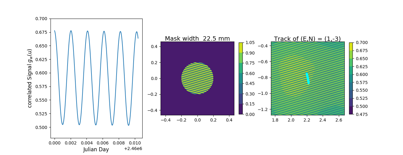
(a) With value of mask’s orientation $104.3^{\circ}$(1.82 radian).

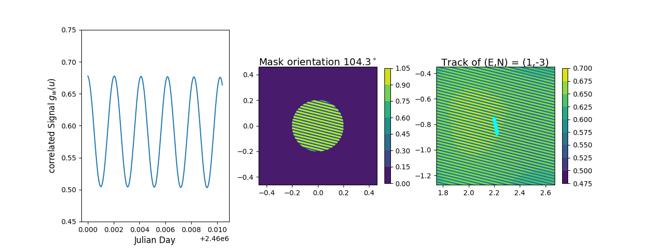
(b) With value of mask’s width 22.5mm.

Figure 1: This figure shows the signal for the mask’s strip width $b=22.5$mm (upper row) and for the mask’s orientation $\hat{\textbf{{u}}}_{0}=104.3^{\circ}$ (lower row). The mask is shown in the middle panels. The underlying correlation $g(\textbf{{u}})$ roughly corresponds to the position of $\alpha\;$Cen AB in 2020, being observed from a latitude of $44^{\circ}\rm\,S$ at a wavelength of $\lambda=$600\text{\,}\mathrm{nm}$$. The right panel shows $g_{\scriptscriptstyle W}(\textbf{{u}})$ on the $\lambda(u,v)$ plane. The cyan tracks correspond to a pair of telescopes with $(\Delta_{\rm E}=$1\text{\,}\mathrm{m}$,\Delta_{\rm N}=$-3\text{\,}\mathrm{m}$)$ over an interval of 15 minutes. The left panel shows $g_{\scriptscriptstyle W}(\textbf{{u}})$ along the cyan tracks. The animated videos of variation in signal with $b$ and $\hat{\textbf{{u}}}_{0}$ are available in the supplementary material.

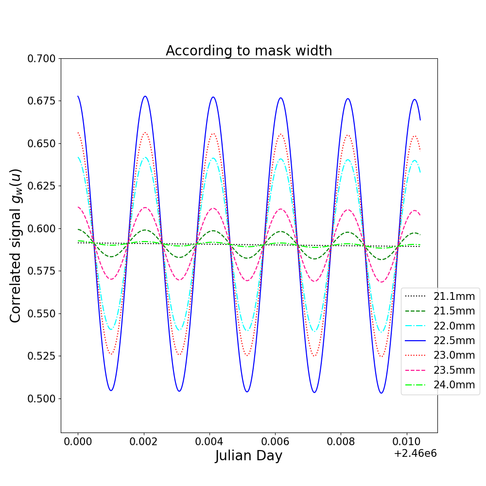
(a) $g_{\scriptscriptstyle W}(\textbf{{u}})$ for different values of $b$.

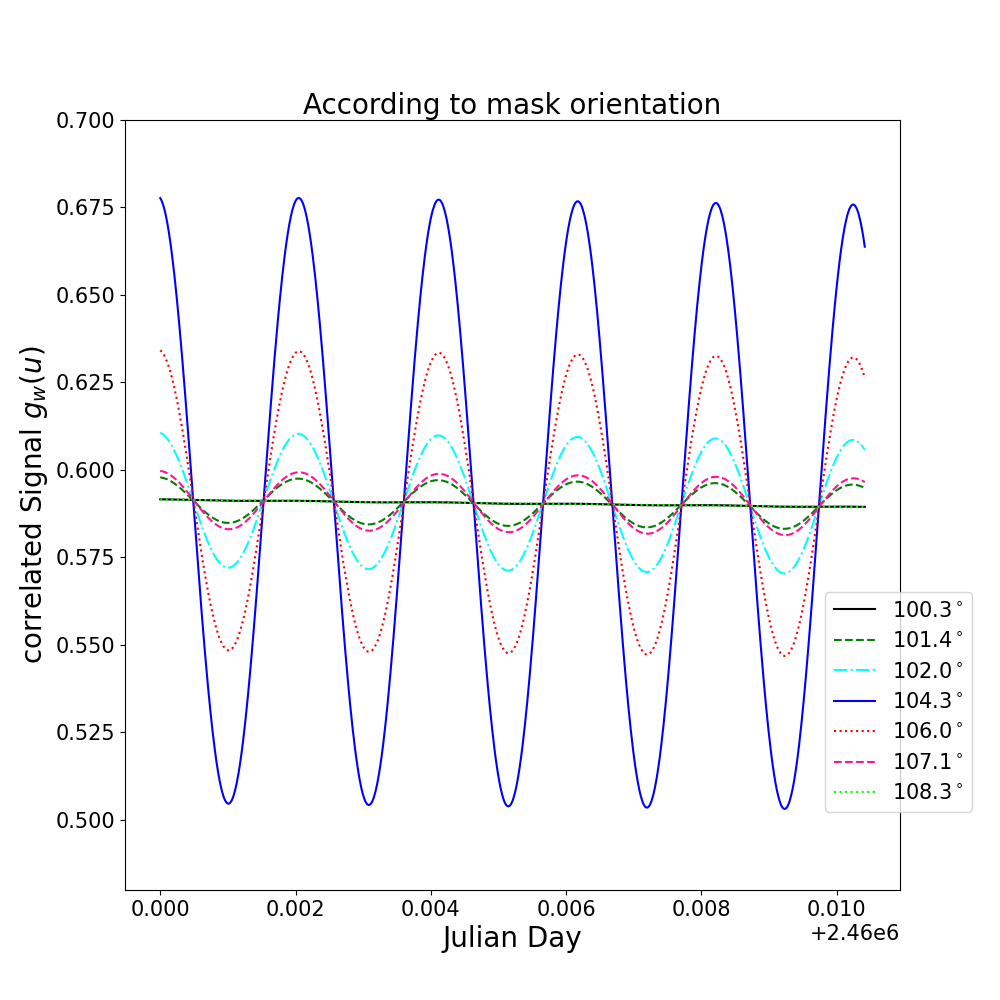
(b) $g_{\scriptscriptstyle W}(\textbf{{u}})$ for different values of $\hat{\textbf{{u}}}_{0}$ .

Figure 2: This figure shows how the aperture mask affects the signal $g_{\scriptscriptstyle W}(\textbf{{u}})$. In the left panel the stripe width $b$ is varied, and in the right panel, the mask orientation $\hat{\textbf{{u}}}_{0}$ is varied. As in Fig 1, the observation time is an interval of 15 minutes with baseline $(\Delta_{\rm E}=$1\text{\,}\mathrm{m}$,\Delta_{\rm N}=$-3\text{\,}\mathrm{m}$)$.

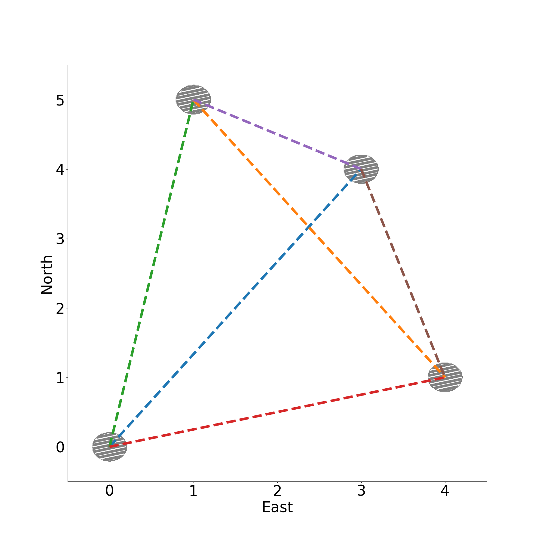
(a) The position of telescopes

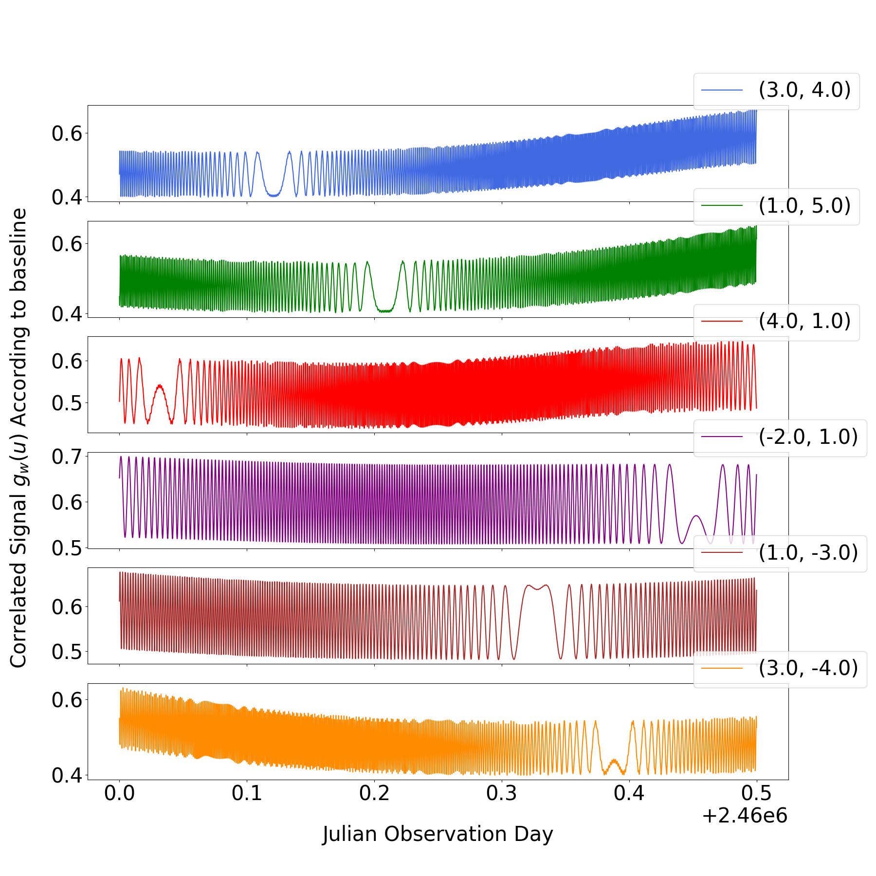
(b) Model signal according to baselines

Figure 3: The left figure shows the position of the four telescopes ((E,N) = (0,0), (1,5), (3,4), (4,1)). The right figure shows the signal according to each baseline for one-night observation. Here the colors of baselines joining the telescope have been taken as the same colors as signals.

Now, the objective plane of a telescope is obviously perpendicular to the line of sight, and hence parallel to the $(u,v)$ plane. We can therefore express the aperture of a telescope as $W(\textbf{{u}})$. The finite-aperture signal is then $g(\textbf{{u}})$ convolved with the apertures of both telescopes. Thus we have

$$g_{\scriptscriptstyle W}(\textbf{{u}})=\frac{\int g(\textbf{{u}}+\textbf{{u}}_{2}-\textbf{{u}}_{1})\,W(\textbf{{u}}_{1})\,W(\textbf{{u}}_{2})\;d^{2}\textbf{{u}}_{1}\,d^{2}\textbf{{u}}_{2}}{\int W(\textbf{{u}}_{1})\,W(\textbf{{u}}_{2})\;d^{2}\textbf{{u}}_{1}\,d^{2}\textbf{{u}}_{2}}$$ (7)

for the finite aperture, and then

$$g^{\rm obs}=\frac{\Delta\tau}{\Delta t}\,g_{\scriptscriptstyle W}(\textbf{{u}})$$ (8)

will be the measured intensity correlation.

The convolution (7) suggests that making $W(\textbf{{u}})$ similar to the fringe pattern itself will prevent the fringes from being washed out. Accordingly we choose

$$W(\textbf{{u}})=\begin{cases}\cos^{2}\Big{(}(\pi\lambda/b)\,\textbf{{u}}\cdot\hat{\textbf{{u}}}_{0}\Big{)}&\text{for}\ \rho\lambda<\tilde{a}\\ 0&\text{otherwise}\end{cases}$$ (9)

which looks complicated, but really just describes a set of sinusoidal stripes inside a circle. Here $\tilde{a}$ denotes the radius of the telescope aperture, $\hat{\textbf{{u}}}_{0}$ is a unit vector and hence, specifies the orientation of the stripes, and $b$ is the stripes width (the length of a stripe will vary according to its position on aperture).

Computation of the convolution (7) is done on a $1024\times 1024$ grid.

Figs. 1 and 2 illustrate the dependence of the signal $g_{\scriptscriptstyle W}(\textbf{{u}})$ on the stripe width $b$ and the orientation $\hat{\textbf{{u}}}_{0}$. For the assumed relative position and the stars and an observing wavelength of $600\text{\,}\mathrm{nm}$, the fringes are most apparent in $g_{\scriptscriptstyle W}(\textbf{{u}})$ for stripe width $b=$2.25\text{\,}\mathrm{cm}$$ and $\hat{\textbf{{u}}}_{0}$ oriented at $104.3^{\circ}$ with respect to u. The signal degrades noticeably when $b$ and $\hat{\textbf{{u}}}_{0}$ are even a few percent from the optimal values. Hence, advance knowledge of the current relative positions of the stars to $\sim 1\%$ is desired, in order to optimise the aperture mask. This is unlikely to be a problem in practice for a wide binary such as the $\alpha\;$Cen AB.

A possible additional complication, depending on the type of telescope mounting, is that the mask may need to be rotated as the telescope tracks the target across the sky, to compensate for field rotation. Equatorial mounting would eliminate this issue.

Four telescopes have been considered during the simulation work. Fig. 3(a) shows their arrangement. Each telescope has a diameter of $40\text{\,}\mathrm{cm}$ and a mask with the optimal aperture mask mentioned earlier. The signal for one-night of observation from all six baselines formed by these four telescopes is shown in Fig. 3(b).

2.3 Signal to Noise

In a resolution time $\Delta t$ the number of HBT correlated photon pairs will be

$$S=(A\Phi)^{2}\;g_{\scriptscriptstyle W}(\textbf{{u}})\times\frac{\Delta t}{\Delta\tau}$$ (10)

where

$$A=\int W(\textbf{{u}})\;d^{2}\textbf{{u}}$$ (11)

is the effective area of each telescope, $\Phi$ is the spectral photon density, and $\Delta\tau$ is the coherence time.

The coherence time is the reciprocal of the frequency bandwidth, thus $1/\Delta\nu=\lambda^{2}/(c\Delta\lambda)$. For the assumed observing wavelength of $600\text{\,}\mathrm{nm}$ the wave period is $\lambda/c=$2.0\text{\,}\mathrm{fs}$$. No specific $\Delta\lambda$ is assumed, but narrow bandwidths are generally desirable. A bandwidth of $\Delta\lambda=$1\text{\,}\mathrm{nm}$$ gives $\Delta\tau=$1.2\text{\,}\mathrm{ps}$$. In practice, $\Delta t$ will be orders of magnitude larger than $\Delta\tau$. The photon spectral density denotes the photons per unit area in a coherence time $\Delta\tau$ in one polarisation, which for a thermal source is given by

$$\Phi=\frac{(\nu/c)^{2}}{e^{z}-1}\times\Delta\Omega\qquad z=\frac{h\nu}{kT}$$ (12)

where $\Delta\Omega$ is the solid-angle area of the source, and $T$ is the effective temperature. The spectral energy flux (measured in Jy) is $2h\nu\Phi$.

In an interval $\Delta t$, the noise due to chance coincidences will be

$$N=A\Phi\times\frac{\Delta t}{\Delta\tau}\,.$$ (13)

Dividing equations (10) and (13) gives the signal to noise of

$${\rm SNR}_{\Delta t}=A\Phi\;g_{\scriptscriptstyle W}(\textbf{{u}})$$ (14)

in one time slice $\Delta t$. We assume $\Delta t=$100\text{\,}\mathrm{ps}$$.

In practice, the correlation would be done in hardware and averaged over an $t_{\rm av}$ during which u can be assumed constant. We take $t_{\rm av}=$1\text{\,}\mathrm{s}$$. This constitutes a data point for fitting. The SNR of such a data point will be

$${\rm SNR}_{t_{\rm av}}=A\Phi\;g_{\scriptscriptstyle W}(\textbf{{u}})\;(t_{\rm av}/\Delta t)^{1/2}\,.$$ (15)

For simulations, one can take the signal to be $g_{\scriptscriptstyle W}$ and the noise to be

$$N=(\Delta t/t_{\rm av})^{1/2}(A\Phi)^{-1}\,.$$ (16)

It is noted that $g_{\scriptscriptstyle W}(\textbf{{u}})$ is several times smaller than $g(\textbf{{u}})$. That is, the aperture mask sacrifices a lot of signal. Let us therefore consider what the SNR would be, if small light buckets without aperture masking were used. For a given effective temperature, $\Phi\propto(R/D)^{2}$, where $R$ is the radius of the larger star and $D$ the distance. If $a$ is the separation between the stars, the width of the interference fringes will be $\propto D/a$. Without aperture masking, the mirror diameter must to kept smaller than the fringe width, implying $A\propto(D/a)^{2}$. This would give ${\rm SNR}\propto(R/a)^{2}$, which becomes hopelessly small for wide binaries. Pointing error is not considered.

3 Orbits

If the $\alpha\;$Cen system has a planet, the observed astrometry of the two bright stars would be part of a four-body system, including the planet and Proxima. We have accordingly carried out orbit integrations of a four-body system of the three stars and a fictitious planet around $\alpha\;$Cen A, with many choices for the planet mass and orbit. Further perturbations, such as the Galactic tidal field, are not expected to be significant, and are not included. The initial conditions are based on orbital parameters from the literature for $\alpha\;$Cen A and B (Pourbaix et al., 2002), and for Proxima with respect to the barycentre of A and B (Kervella et al., 2017b).

$M$ ($M_{\odot}$)	$P$ (yr)	$a$ (au)	$e$	$\iota$ (deg)	$\Omega$ (deg)	$t_{\rm peri}$ (yr)	$\omega$ (deg)
1.1
$10^{-2}$	1	1	0	80	0	0	0
0.9	79.9	23.5	0.518	79	204.85	1875.66	231.65
0.1221	547000	8700	0.5	107	126	285000	72

Table 1: Masses $M$ and orbital elements (Period $P$, semi-major axis $a$, eccentricity $e$, inclination $\iota$, longitude of the ascending node $\Omega$, periastron epoch ($t_{\rm peri}$), and argument of periapsis $\omega$) for the $\alpha\;$Cen system. The top line is for $\alpha\;$Cen A. The second line represents a fictitious planet. The third line gives the observed orbit of the $\alpha\;$Cen AB system (Pourbaix et al., 2002), while the last line gives the orbit of Proxima Centauri with respect to the barycentre of the two bright stars (Kervella et al., 2017b).

3.1 The Orbital Integration

The equations of motion of an $N$-body system with masses $m_{i}$ ($i=0,1,\ldots,N-1$) in terms of the positions $\textbf{{X}}_{i}$ and velocities $\textbf{{V}}_{\!i}$ in an inertial reference frame are given by:

$$\ddot{\textbf{{X}}_{i}}\equiv\dot{\textbf{{V}}_{\!i}}=-\sum_{j=0;j\neq i}^{N-1}Gm_{j}\frac{\textbf{{X}}_{i}-\textbf{{X}}_{j}}{|\textbf{{X}}_{i}-\textbf{{X}}_{j}|^{\hbox to0.0pt{$\scriptstyle 3$\hss}}}$$ (17)

where $G$ is the gravitational constant.

We use the well known Leapfrog algorithm, also otherwise known as Drift-Kick-Drift, or the Verlet method, to solve for the orbits of this system. Under this algorithm, the set of phase space vectors $\{(\textbf{{X}}_{i}(t),\textbf{{V}}_{\!i}(t)),i=0,1,\ldots,N-1\}$ are advanced by the following set of steps:

$$\textbf{{X}}_{i}^{\rm int} =\textbf{{X}}_{i}^{\rm old}+\ \textbf{{V}}_{\!i}^{\rm old}\times{\textstyle\frac{1}{2}}t_{\rm step}$$ (18)

$$\textbf{{V}}_{\!i}^{\rm new} =\textbf{{V}}_{\!i}^{\rm old}-{\sum_{j=0,j\neq i}^{N-1}Gm_{j}}\frac{\textbf{{X}}_{i}^{\rm int}-\textbf{{X}}_{j}^{\rm int}}{|\textbf{{X}}_{i}^{\rm int}-\textbf{{X}}_{j}^{\rm int}|^{\hbox to0.0pt{$\scriptstyle 3$\hss}}}\,\times t_{\rm step}$$

$$\textbf{{X}}_{i}^{\rm new} =\textbf{{X}}_{i}^{\rm int}+\ \textbf{{V}}_{\!i}^{\rm new}\times{\textstyle\frac{1}{2}}t_{\rm step}.$$

The first step (Drift) in equation (18) produces an interim position vector $\textbf{{X}}_{i}^{\rm int}$ using the present values of the position vector $\textbf{{X}}_{i}^{\rm old}$ and the velocity vector $\textbf{{V}}_{\!i}^{\rm old}$ over half the chosen time step, i.e., $\frac{1}{2}t_{\rm step}$. The second step (Kick) is produced by generating the next set of velocity vectors $\textbf{{V}}_{\!i}^{\rm new}$ over a full time step $t_{\rm step}$ by using the accelerations evaluated at the interim position vectors $\textbf{{X}}_{i}^{\rm int}$. Finally, in the last step (a second Drift), the next set of position vectors $\textbf{{X}}_{i}^{\rm new}$ are evaluated with the remaining half a time step $\frac{1}{2}t_{\rm step}$ using the set of velocity vectors $\textbf{{V}}_{\!i}^{\rm new}$ at the next time step. More efficient algorithms are available (Mikkola, 2020), but Leapfrog is sufficient for our purposes. It is known to conserve momentum and angular momentum exactly. The total energy has an oscillatory variation proportional to $(t_{\rm step})^{2}$ and no secular variation.

Light-second units have been used for the computation. That is done by making the code variables $\textbf{{X}}_{i}/c$ and $\textbf{{V}}_{\!i}/c$, and mass parameters in the program $Gm_{i}/c^{3}$. The time step is $t_{\rm step}=$1\text{\times}{10}^{6}\text{\,}\mathrm{s}$$.

3.2 Initial conditions

Table 1 gives the masses and orbital elements of the stars, taken from the literature, and (in the second) line the parameters for a fictitious planet.

Orbital elements such as in Table 1 describe instantaneous two-body orbits. They can be transformed to cartesian positions and velocities by the following procedure (for a derivation, see e.g., Saha & Taylor, 2018).

First we solve Kepler’s equation

$$\psi-e\sin\psi=\frac{2\pi}{P}(t-t_{\rm peri})$$ (19)

for the eccentric anomaly $\psi$ with $t_{\rm peri}$ being the epoch of periastron of the system. We then use the value of $\psi$ to compute the position in the orbital plane, and then we apply three rotations

$$\begin{pmatrix}x\\ y\\ z\end{pmatrix}=a\times R_{3}(\Omega)\,R_{1}(\iota)\,R_{3}(\omega)\begin{pmatrix}\cos\psi-e\\ \sqrt{1-e^{2}}\sin\psi\\ 0\end{pmatrix}$$ (20)

so as to orient the coordinates conveniently with $z$ along the line of sight. In equation (20), the set of parameters {$a$, $e$, $\iota$, $\Omega$ and $\omega$} represent the standard Keplerian orbit elements noted in table 1. The $R_{1}$ matrices are as in equation (5), and $R_{3}$ is given by cyclically permuting the indices. The analogous expression for velocities follows by noting

$$\frac{d\textbf{{x}}}{dt}=\frac{2\pi}{P}\frac{d\textbf{{x}}}{d\psi}$$ (21)

which itself follows from equation (19).

Applying the above procedure to the orbital elements, gives us three positions $\textbf{{x}}_{1},\textbf{{x}}_{2},\textbf{{x}}_{3}$ and three corresponding velocities. These are two-body coordinates and velocities, and correspond to pairs of bodies, not individual bodies. We now interpret these as Jacobi variables. That is, $\textbf{{x}}_{1}$ is considered as the position of the second body (the fictitious planet) with respect to the first body ($\alpha\;$Cen A), $\textbf{{x}}_{2}$ is taken from the third body ($\alpha\;$Cen B) to the barycentre of the earlier bodies, and so on. Inertial coordinates $\textbf{{X}}_{i}^{I}$ are then given by

$$\textbf{{X}}_{0}^{I} =0$$ (22)

$$\textbf{{X}}_{i}^{I} =\textbf{{x}}_{i}+\frac{\sum_{j<i}m_{j}\textbf{{X}}_{j}^{I}}{\sum_{j<i}m_{j}}$$

and similarly for velocities. Finally the positions and velocities are transformed to barycentric coordinates

$$\textbf{{X}}_{i}=\textbf{{X}}_{i}^{I}-\frac{\sum_{j}m_{j}\textbf{{X}}_{j}^{I}}{\sum_{j}m_{j}}$$ (23)

and again similarly for velocities.

3.3 The simulated orbits

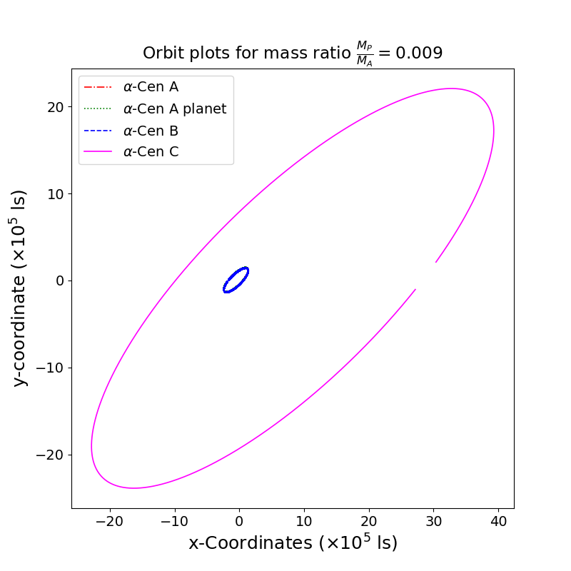
(a) Orbit of $\alpha\;$Cen system

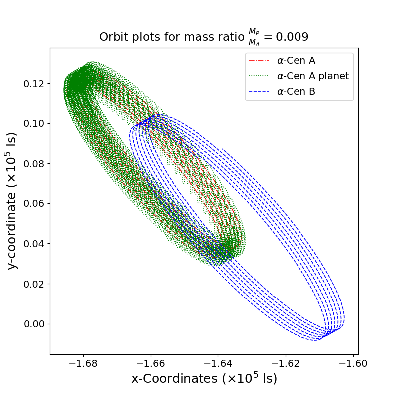
(b) Orbit of $\alpha\;$Cen AB system with a planet

Figure 4: Left: a four-body system ($\alpha\;$Cen system with a planet) for the time duration $\approx$ 0.545 Myr. Right: the orbit of the binary system ($\alpha$-Cen AB) with the planet for a period of $\approx$ 580 yr. The parameters of these objects are provided in Table 1.

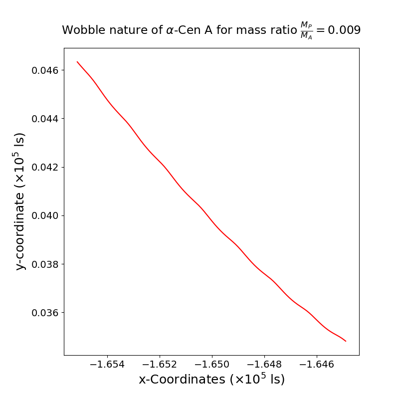
(a) Orbit of $\alpha\;$Cen A for $\approx$ 6 yr of orbit.

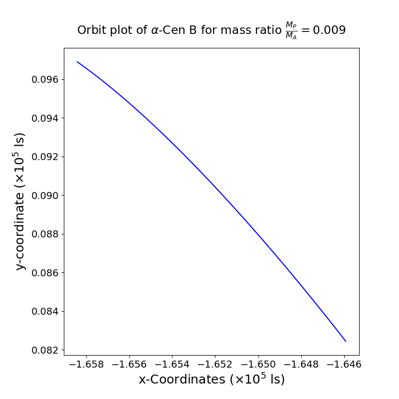
(b) Orbit of $\alpha\;$Cen B for $\approx$ 6 yr of orbit.

Figure 5: This figure is the orbit plot of $\alpha\;$Cen A and $\alpha\;$Cen B for $\approx$ 6 yr of orbit. The left figure shows the perturbation in the orbit of $\alpha\;$Cen A as the ten Jupiter mass planet is revolving in 1 AU semi-major axis orbit around it. The perturbation in the trajectory of $\alpha\;$Cen B (right figure) is not perceptible as (1) there is no planet around it and (2) the perturbations due to the perturbed motion of $\alpha\;$Cen A is expected to be of higher order.

Fig 4 and Fig 5 show the result of integration of equation (17) using leapfrog method. The initial condition and other parameters of all four objects have been taken from table 1. Fig 4 shows the orbit of $\alpha\;$Cen A, $\alpha\;$Cen B, and planet (10 Jupiter mass) in red (dashed-dotted), blue (dashed), and green (dotted) colors, respectively. There is also an orbit of Proxima Centauri in magenta color (solid line), which is situated very far away from the barycenter of these three objects. These orbital solution is obtained by integrating the equations of motion equation (18) for a period of $\approx$ 0.545 Myr. The orbit of the $\alpha\;$Cen AB system is not distinguishable in Fig 4(a) as the separation of Proxima Centauri from the binary system is large enough. The orbit plot of $\alpha\;$Cen AB with a planet has been shown in Fig 4(b). As the Proxima Centauri is gravitationally bounded with $\alpha\;$Cen AB binary (Kervella et al., 2017b), the orbit’s shift of the binary system comes into the picture as a result.

Fig 5(a) shows the trajectory of $\alpha\;$Cen A with respect to the centre of mass of the $\alpha\;$Cen AB -plus-planet system for a period of $\approx$ 6 years. The planet (with ten Jupiter mass) revolves around $\alpha\;$Cen A in 1 AU semi-major axis; the perturbation effect can be seen in this figure. Fig 5(b) shows the trajectory of $\alpha\;$Cen B for the same period. It may be expected that the perturbation in the trajectory of $\alpha\;$Cen B may be imperceptible as (1) there is no planet around it and (2) the perturbations due to the perturbed motion of $\alpha\;$Cen A should be of higher order.

4 Results

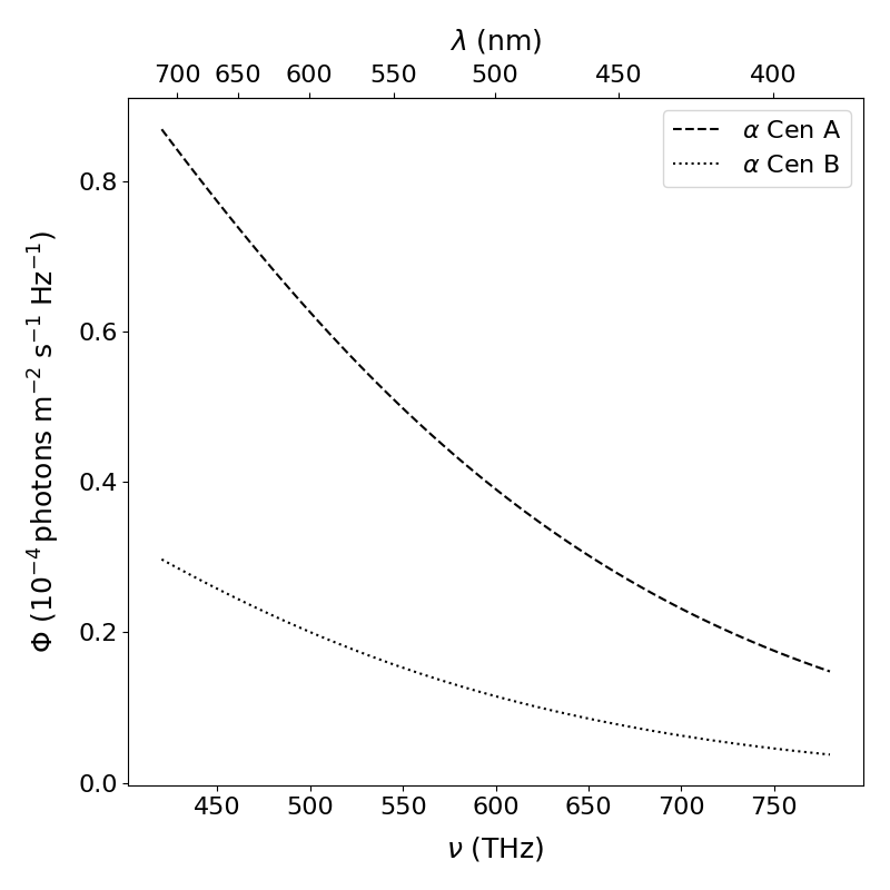
Figure 6: Spectral photon flux in each polarisation for two blackbody sources approximating $\alpha\;$Cen A and B. These are simply the spectral energy density divided by $2h\nu$. Both curves peak in the infrared range, outside the range of the figure. The quantity $\Phi$ used in the simulations is the sum of the two sources evaluated at $600\text{\,}\mathrm{nm}$.

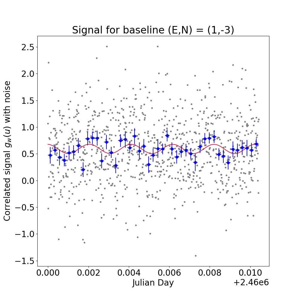
Figure 7: This figure shows the signal $g_{\scriptscriptstyle W}(\textbf{{u}})$ and noise for one baseline with 10 spectral channels. The duration shown is $15\,$min. The grey dots are noisy data in bins of $1\,$s. The blue error bars represent the noisy data in bins of $20\,$s, and the crimson line represents the noiseless signal.

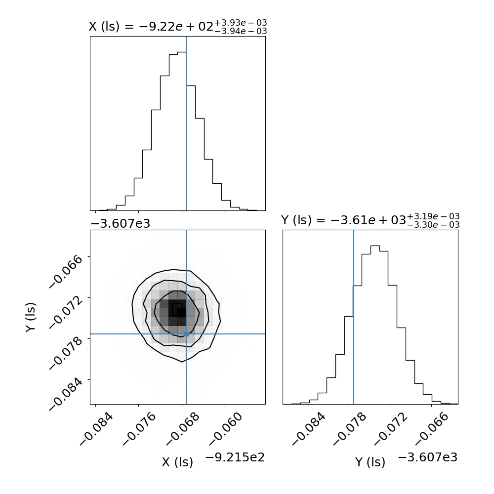
Figure 8: Estimation of the sky-projected relative position $(X,Y)$ $\alpha\;$Cen A,B, with SNR corresponding to observing with 10 spectral channels for 1000 nights. The error is less than $10\,\mu\rm as$ (which corresponds to $7\text{\times}{10}^{-3}\text{\,}\rm\mathrm{l}\mathrm{s}$ at the distance of $\alpha\;$Cen).

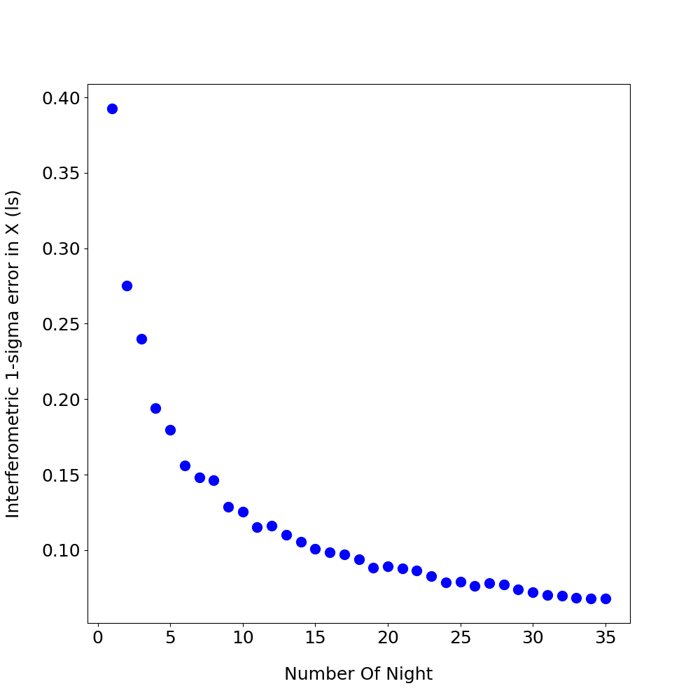
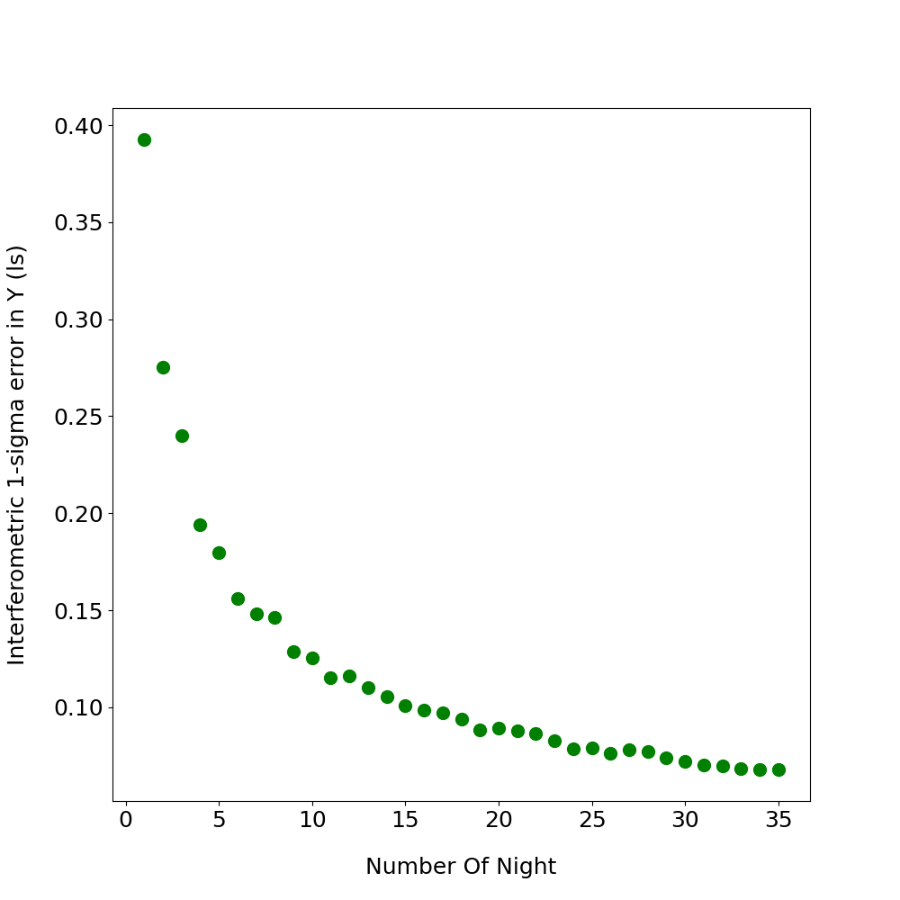
Figure 9: This figure shows the reduction in astrometric error with an increasing number of nights of observation. One channel is assumed. The left panel shows the error in the $X$ coordinate of the binary, and the right panel shows the error in $Y$.

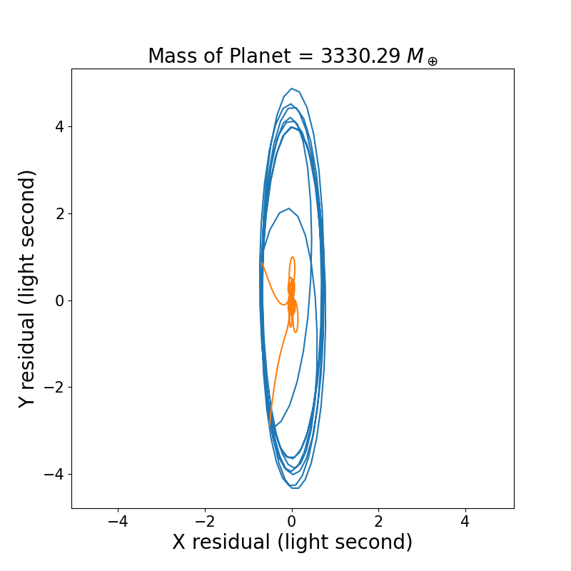
Figure 10: Astrometric wobble over approximately $6\,$yr, corresponding to the orbit shown in Fig. 5(a). Blue: residuals ($\widetilde{X}(t),\widetilde{Y}(t)$) after removal of a polynomial up to $t^{6}$. Orange: residuals ($\Delta\widetilde{X}(t),\Delta\widetilde{Y}(t)$) after further removal of the largest periodic part. This example assumed an implausibly high planet mass ($\approx 10\,M_{\rm Jup}$) to make the wobble perceptible (Fig. 5(a)).

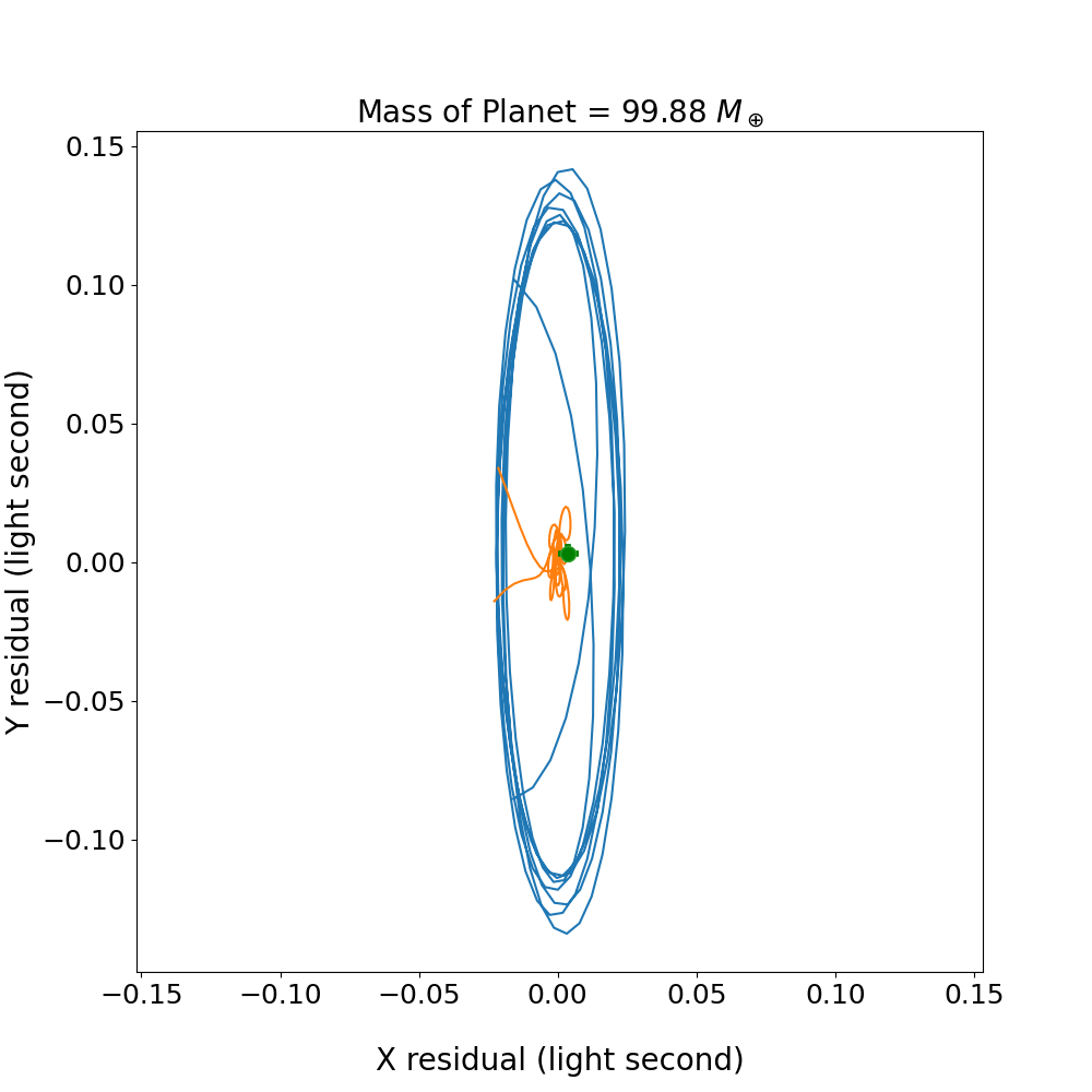
(a) For a Saturn mass planet

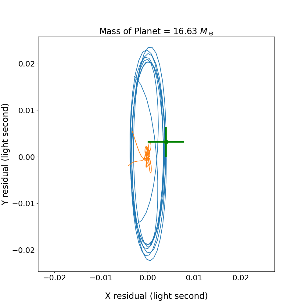
(b) For a Neptune mass planet

Figure 11: This figure shows the residuals with an interferometric error bar. The interferometric bar and also residuals have been taken for different masses.The animated video of residuals with different planet masses is available in the supplementary material.

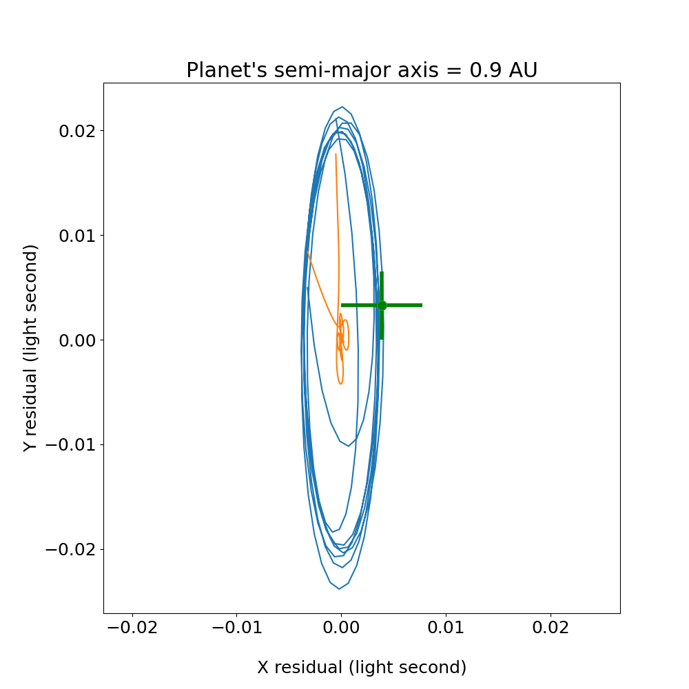
(a) Planet’s estimated period = 0.841 yr

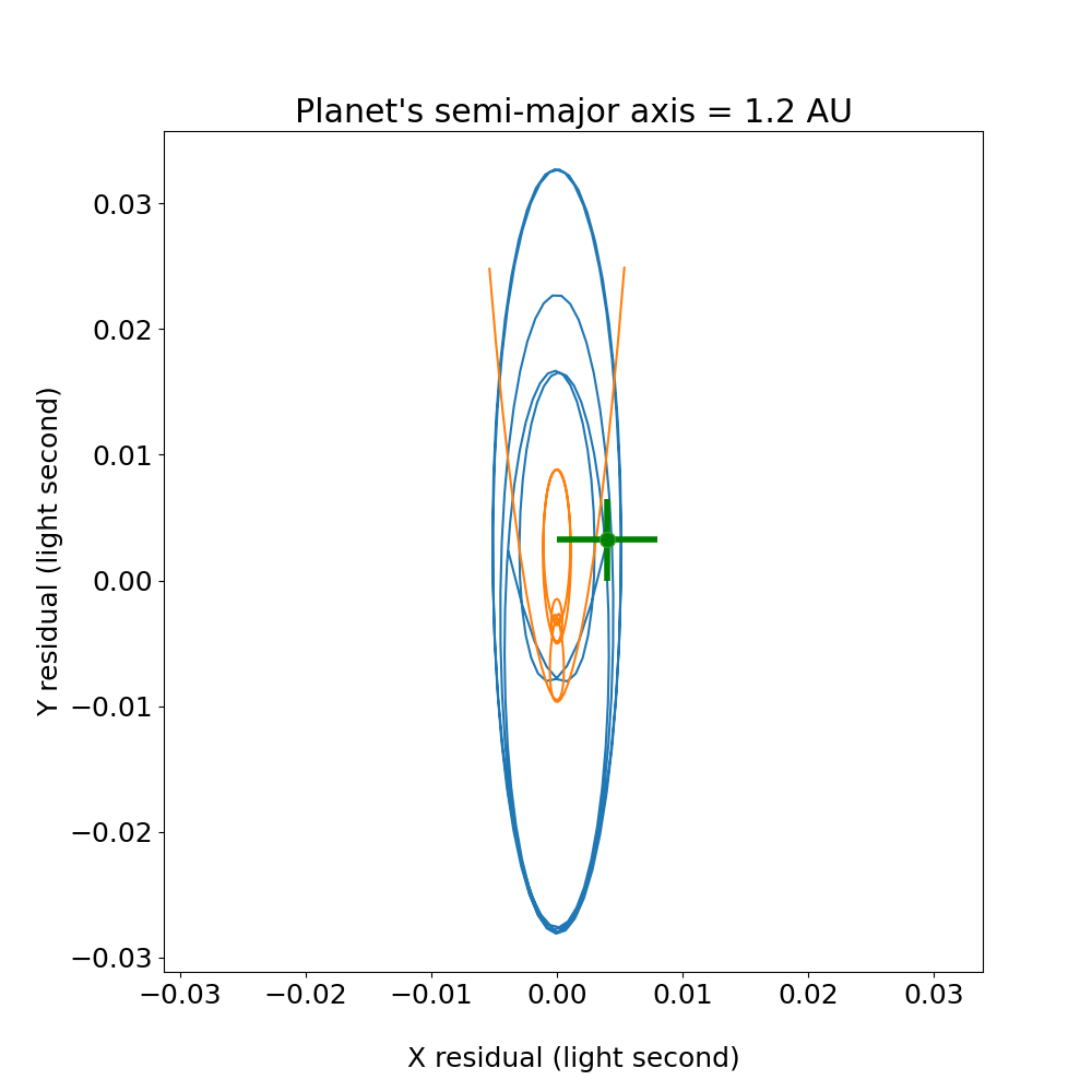
(b) Planet’s estimated period = 1.281 yr

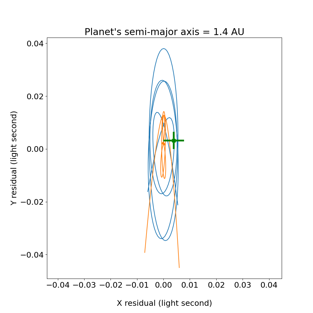
(c) Planet’s estimated period = 1.612 yr

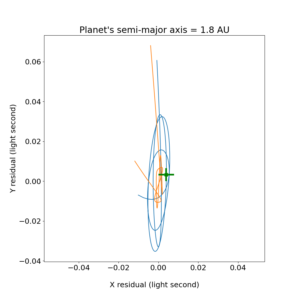
(d) Planet’s estimated period = 2.221 yr

Figure 12: This figure shows the Habitable orbit estimation of the planet, which can be detected using the setup according to the Fig 3(a). The green error bar is the interferometric error. The mass of the planet taken here is Neptune mass and $6^{th}$ order of polynomial for fitting. The estimated periods of the planet according to their Habitable position are (a) 0.841 years, (b) 1.281 years, (c) 1.612 years, (d) 2.221 years.

We now simulate the measurement of the sky-projected relative position $(X,Y)$ of $\alpha\;$Cen A and B from intensity interferometry at an arbitrary epoch in 2023, at various SNR levels. We will then compare the errors on such a measurement with the astrometric wobble in $(X,Y)$ due to a planet with different assumed masses. The distance to the system is assumed known.

A full analysis pipeline would fit for the masses and initial conditions as $X(t),Y(t)$ evolve, rather than for a single-epoch $X,Y$. From astrometric data alone, the inferred parameters will have a degeneracy depending on the assumed value of $D$. Including kinematic data (not necessarily at very high resolution) would allow $D$ to be measured as well. A many-parameter fit combining astrometric and kinematic data would be rather complicated, but is not expected to be intractable. Indeed, an early example of this type of fit appears already in Herbison-Evans et al. (1971).

In this work, however, our main aim is simply to estimate the uncertainty in $X$ and $Y$, and how it depends on the SNR. Thus we do not include the orbital variation of $X$ and $Y$ in the astrometric fitting process. We consider a single-epoch $X,Y$ even though the observing campaign runs over a long time.

4.1 The observing configuration

The setup used is according to Fig. 3(a). Four identical telescopes are arranged a few metres from each other. The diameter of each telescope is $40\text{\,}\mathrm{cm}$, with a mask width $b=$2.25\text{\,}\mathrm{cm}$$ (see equation 9) oriented at $104.3^{\circ}$, so as to approximately match the fringes at the assumed observing wavelength of $600\text{\,}\mathrm{nm}$.

The parameters that set the SNR are as follows.

$$\Phi \simeq$1\text{\times}{10}^{-4}\text{\,}{\rm photons}\;\mathrm{m}^{-2}\,\mathrm{s}^{-1}\,\mathrm{Hz}^{-1}$$$ (24)

$$A \simeq$0.05\text{\,}\mathrm{m}^{2}$$$

$$\Delta t \simeq$1\text{\times}{10}^{-10}\text{\,}\mathrm{s}$\,.$$

The spectral photon density $\Phi$ at the observing wavelength follows from the effective temperatures and angular sizes of the stars (see Fig. 6). The assumed time resolution $\Delta t$ appears realistic and has even been surpassed (cf. Horch et al., 2022). With these parameters, equation (15) gives

$${\rm SNR}\simeq 0.5\times g_{\scriptscriptstyle W}(\textbf{{u}})\times{\rm channels}^{1/2}\times(\hbox{$t_{\rm obs}$ in s})^{1/2}\,.$$ (25)

That is to say, if each data point corresponds to $t_{\rm av}=1\rm\,s$, noise with $\sigma\simeq 2$ would be added to Fig. 3(b).

These estimates neglect throughput and detector efficiency. In real life, these could easily reduce the SNR by a factor of two. However, such losses could be compensated for by increasing the diameter of the telescopes to say 60 cm.

Fig. 7 shows some detail of the simulated noisy data. The Earth’s rotation causes the baseline to cross fringes on the $(u,v)$ plane. Over $1\,$s the SNR is less than unity. With $20\,$s bins a fringe pattern is barely noticeable. With enough accumulated data, however, the pattern can be fitted with high precision.

4.2 Astrometric fitting

We now apply Bayesian parameter fitting to infer $(X,Y)$ from the observable (Eq. 8) with noise. Assuming Gaussian noise with rms $\sigma$, the likelihood will be $\exp(-\frac{1}{2}\chi^{2})$, where

$$\chi^{2}=\sigma^{-2}\sum_{k}\left(g^{\rm obs}_{k}-\frac{\Delta\tau}{\Delta t}g_{\scriptscriptstyle W}(\textbf{{u}}_{k})\right)^{2}$$ (26)

and $g^{\rm obs}_{k}$ is the signal (equation 8) at the $k^{th}$ data point for the $u_{k}$ baseline. $g_{\scriptscriptstyle W}(\textbf{{u}})$ depends on $X/D,Y/D$ through Equations. (2) and (3).

There are two distinct time dependencies that go into $g_{\scriptscriptstyle W}(\textbf{{u}})$. One is the fast time variation illustrated in Fig. 3(b) as the Earth rotates and u changes. This variation is what allows the fringes to be measured and hence the astrometry to be inferred. Then there is a slow variation of $X$ and $Y$ as indicated in Fig. 5(a) as the stars move in their orbits.

To fit for $X,Y$ we use dynamic nested sampling (Skilling, 2004, 2006) as implemented in the dynesty code Speagle (2020). The normalisation constant $\Delta\tau/\Delta t$ is marginalised out (see e.g., Eq. 29–33 of Rai et al., 2021) to avoid having to fit for it.

As an ambitious but still realistic scenario, consider an observing program of 1000 nights using 10 spectral channels using the setup of Fig. 3(a). This would be time series $10^{4}$ times what is illustrated in Fig. 3(b). The stellar positions would change during this time, necessitating ongoing modifications of the mask. In this work we do not attempt to simulate and fit such a large data set. Instead we take the signal for one channel and one night (as in Fig. 3(b)) and add only 1/100 of the noise level for one night. That is, we take the data for one night and reduce the noise by $({\rm channels}\times{\rm nights})^{1/2}$, compared to equation (16). The total SNR is about $14140$. Fig. 8 shows the resulting estimation of $(X,Y)$ in light-seconds. At $D=1.4\,$pc a light-second is about $\approx 1.5\,$mas. The 60% uncertainties along East-West and North-South are $\approx 5.3\mu\rm as$ and $\approx 6.2\mu\rm as$ respectively, which is comparable to the astrometric perturbation due to an Earth-mass planet $1\text{\,}\rm\mathrm{a}\mathrm{u}$ from the $\alpha\;$Cen A.

As a check that our simplification of simply reducing the noise level to mimic a longer observing run is reasonable, we have carried out simulations of one channel up to 35 nights. The result is shown in Fig. 9, we see that the accuracy indeed improves according to ${\rm nights}^{-1/2}$ as expected.

4.3 The astrometric wobble

The observable signal is the difference between the trajectories on the sky of $\alpha\;$Cen A and B, which is to say, the difference between the two panels of Fig. 5. Over a few years, the motion is mainly an arc of the 80 yr binary orbit of $\alpha\;$Cen A-B. The planetary motion causes a very small wobble, which is barely visible in Fig. 5 despite the unrealistically large planetary mass assumed. To extract the wobble, we subtract out a best-fit polynomial

$$X(t) =X_{0}+X_{1}t+X_{2}t^{2}+X_{3}t^{3}+X_{4}t^{4}+X_{5}t^{5}+X_{6}t^{6}$$ (27)

$$+\widetilde{X}(t)$$

$$Y(t) =Y_{0}+Y_{1}t+Y_{2}t^{2}+Y_{3}t^{3}+Y_{4}t^{4}+Y_{5}t^{5}+Y_{6}t^{6}$$

$$+\widetilde{Y}(t)$$

leaving a residual $\widetilde{X}(t),\widetilde{Y}(t)$, which we call the astrometric wobble. The polynomial fit was chosen after some trials as 6-th degree. The wobble was further fitted to a sinusoid

$$\widetilde{X}(t) =X_{7}\cos(\omega t)+X_{8}\sin(\omega t)+\Delta\widetilde{X}(t)$$ (28)

$$\widetilde{Y}(t) =Y_{7}\cos(\omega t)+Y_{8}\sin(\omega t)+\Delta\widetilde{Y}(t)$$

leaving a smaller residual $\Delta\widetilde{X}(t),\Delta\widetilde{Y}(t)$. The fitted $\omega$ is the inferred angular frequency of the planet around its host star.

Fig. 10 shows the wobble $\widetilde{X}(t),\widetilde{Y}(t)$ and the residual $\Delta\widetilde{X}(t),\Delta\widetilde{Y}(t)$ corresponding to the orbit in Fig. 5. The blue curve in Fig. 10 is, in effect, the reflex motion of the host star due to the planetary orbit Fig. 4(b), in a coordinate system that follows the smoothed motion of the host star. The fitted value of the planet’s period is 0.841 yr, which differs from the input value in Table 1 because of orbital perturbations. The highly eccentric appearance is partly due to projection, but is also partly due to the perturbation from $\alpha\;$Cen B.

4.4 Threshold mass and habitable orbit

Fig. 11 shows the astrometric wobble along with an interferometric error bar (cf. Fig. 8). The wobble residuals (blue and orange) and the interferometric error bar (green) vary according to the planet’s masses.

As the planet’s mass is in the range of Jupiter mass or lower, the perturbed residual is more than the interferometric error. For the mass range 3330–3$\,M_{\oplus}$ the typical $\widetilde{Y}$ is larger than the interferometric error. However, the typical $\widetilde{X}$ becomes comparable to the interferometric error for masses lower than about 16$\,M_{\oplus}$ ($\approx$Neptune mass).

Thus the detection threshold for the assumed setup in Fig. 3(a) is roughly a Neptune-mass planet in an Earth-like orbit.

Studies have been shown that habitable zones exist in the $\alpha\;$Cen AB system (different for both stars). The range for $\alpha\;$Cen A is (0.9–2.2) au and for $\alpha\;$Cen B is (0.5-1.3) au as semi-major axis Belikov et al. (2015).

Fig12 shows the estimation of orbit and period in the habitable zone for $\alpha\;$Cen A with Neptune mass of a planet. The variation in blue $\widetilde{X},\widetilde{Y}$ and orange $\Delta\widetilde{X},\Delta\widetilde{Y}$ are according to their increased semi-major axis from $\alpha\;$Cen A. As before the green error bars represent the interferometric error.

4.5 Inferring the host star

The observable signature of a planet around one of $\alpha\;$Cen A or B, would be that the relative vector between the two stars exhibits an approximately Keplerian orbit with (say) semi-major axis $a_{w}$ and angular frequency $\omega$. (There will be an uncertainty in $a_{w}$ because the inclination is not known a priori, but let us suppose the inclination is adequately constrained by stability arguments.) These observable quantities are given by

$$a_{w}=\frac{m}{M_{1}}a_{p}$$ (29)

and

$$\omega^{2}=\frac{G(M_{1}+m)}{a_{p}^{3}}$$ (30)

where $m$ denotes the mass of the planet, $M_{1}$ that of the host star, and $a_{p}$ the orbital semi-major axis. Combining these we have

$$Gm(1+m/M_{1})^{1/3}=(GM_{1}\omega)^{2/3}\,a_{w}$$ (31)

which determines the mass of the planet provided $M_{1}$ is known. The trouble is, while the masses of $\alpha\;$Cen A and B are known, it is not known which of them is $M_{1}$, which leaves a curious degeneracy in $m$.

Nevertheless, it seems plausible that the true host star could be inferred, because of the perturbations of the other star. The apparent orbit would show three-body perturbations from Keplerian. The strength of the perturbations would depend on $a_{p}/r_{\rm tid}$ where $r_{\rm tid}$ is a characteristic scale for tidal perturbations. Let us put

$$r_{\rm tid}=(M_{1}/M_{2})^{1/3}\,r_{\scriptscriptstyle\!AB}$$ (32)

where $r_{\scriptscriptstyle\!AB}$ is the current distance of the other star and $M_{2}$ is its mass. The expression for $r_{\rm tid}$ is simply the usual Hill radius, apart from a factor of $3^{1/3}$. Combining with equations (29) and (30) and neglecting the tiny term $m/M_{1}$, we have

$$\frac{a_{p}}{r_{\rm tid}}=\left(\frac{GM_{2}}{\omega^{2}}\right)^{1/3}\frac{1}{r_{\scriptscriptstyle\!AB}}$$ (33)

for the amplitude of perturbations.

The above considerations suggest that determining which star is the host from three-body perturbations would be much harder still than detecting a planet via astrometry, if indeed a planet is present, but not hopeless.

5 DISCUSSION

Astrometry to accuracies beyond what is currently available would be a means to detect or rule out a habitable planet in the $\alpha\;$Cen system. This paper studies intensity interferometry as a possible means to this end. As usual with intensity interferometry, high-end photon detectors and correlators are required, and accumulating enough SNR takes a long time. But set against these is the advantage of a very simple optical setup, requiring only amateur-grade telescope and no special infrastructure, because coherence between optical elements is not required.

Herbison-Evans et al. (1971) used intensity interferometry for astrometry of $\alpha\,$Virginis (Spica). Recently in Rai et al. (2021) an extension to measure the radii of both stars together has been suggested. But this will not work for wide binary like $\alpha\;$Cen. As explained in Section 2 the requirement that the light buckets are smaller than the fringe width implies that ${\rm SNR}\propto(R/a)^{2}$ where $a$ is the separation between the stars and $R$ is the radius of the larger star. For Spica $a/R\sim 10$ whereas for $\alpha\;$Cen $a/R>10^{3}$.

To evade this problem, we suggest a sort of matched filter in the form of a mask placed on the objective. For large apertures, the mask could also be placed in secondary optics.

With a declination of $-60^{\circ}\,50^{\prime}$ $\alpha\;$Cen is observable year-round from latitudes further South than $30^{\circ}\,$S. The $1.8\text{\,}\mathrm{m}$-MOA telescope (see e.g., Hearnshaw et al., 2006) at Mt. John Observatory in New Zealand can observe $\alpha\;$Cen throughout the year, but at present is not set up for interferometry. Hence we consider a different scenario, with small portable telescopes at a nearby location, but dedicated to $\alpha\;$Cen. Horch et al. (2022) have recently demonstrated intensity interferometry with movable 60 cm telescopes, including multi-channel correlation, so a basis for our assumed setup is already available. Adding aperture masks with appropriate stripe width and orientations to do orbital astrometry by $<$10\text{\,}\mathrm{\SIUnitSymbolMicro}{\rm as}$$ levels, is still a problem to be addressed; 3D printing may be a route to achieve this goal.

Data Availability

The data underlying this article are available in the article and in its online supplementary material.

References

- Abuter et al. (2017) Abuter R., et al., 2017, A&A, 602, A94
- Anglada-Escudé et al. (2016) Anglada-Escudé G., et al., 2016, Nature, 536, 437
- Beichman et al. (2020) Beichman C., et al., 2020, PASP, 132, 015002
- Belikov et al. (2015) Belikov R., Bendek E., Thomas S., Males J., 2015, in Pathways Towards Habitable Planets. p. 101
- Bendek et al. (2021) Bendek E., Mamajek E., Vasisht G., Tuthill P., Belikov R., Nielsen E., Toliman Team 2021, in American Astronomical Society Meeting Abstracts. p. 318.02
- Benest (1988) Benest D., 1988, A&A, 206, 143
- Catanzarite et al. (2008) Catanzarite J., Law N., Shao M., 2008, in Optical and Infrared Interferometry. p. 70132K
- Claret & Hauschildt (2003) Claret A., Hauschildt P. H., 2003, A&A, 412, 241
- Curiel et al. (2020) Curiel S., Ortiz-León G. N., Mioduszewski A. J., Torres R. M., 2020, AJ, 160, 97
- Damasso et al. (2020) Damasso M., et al., 2020, Science Advances, 6, eaax7467
- Hatzes (2002) Hatzes A. P., 2002, Astronomische Nachrichten, 323, 392
- Hearnshaw et al. (2006) Hearnshaw J. B., et al., 2006, in Sutantyo W., Premadi P. W., Mahasena P., Hidayat T., Mineshige S., eds, The 9th Asian-Pacific Regional IAU Meeting. p. 272 (arXiv:astro-ph/0509420)