Spin-induced dynamical scalarization, de-scalarization and stealthness
in scalar-Gauss-Bonnet gravity during black hole coalescence

Abstract

Particular couplings between a scalar field and the Gauss-Bonnet invariant lead to spontaneous scalarization of black holes. Here we continue our work on simulating this phenomenon in the context of binary black hole systems. We consider a negative coupling for which the black-hole spin plays a major role in the scalarization process. We find two main phenomena: (i) dynamical descalarization, in which initially scalarized black holes form an unscalarized remnant, and (ii) dynamical scalarization, whereby the late merger of initially unscalarized black holes can cause scalar hair to grow. An important consequence of the latter case is that modifications to the gravitational waveform due to the scalar field may only occur post-merger, as its presence is hidden during the entirety of the inspiral. However, with a sufficiently strong coupling, we find that scalarization can occur before the remnant has even formed. We close with a discussion of observational implications for gravitational-wave tests of general relativity.

I Introduction

The detection of gravitational waves (GW) produced by coalescing compact binaries by the LIGO-Virgo-Kagra Collaboration [1, 2, 3] have opened a new avenue to test general relativity (GR) in its strong-field, nonlinear regime [4, 5, 6, 7, 8]. In fact, the first three catalogs of observations have already been used to perform several null tests of GR [8, 9, 10, 11, 12, 13, 14, 15, 16, 17], as well as theory-specific tests [18, 19, 20, 21, 20, 22, 23, 24, 25, 19, 26]. The latter have placed constraints on quadratic gravity theories [22, 23, 24, 25, 21].

In these theories, a scalar field couples to a curvature scalar, which is quadratic in the Riemann tensor (see e.g. Ref. [27] for an overview). Well-known examples include coupling to the Pontryagin density or the Gauss-Bonnet (GB) invariant. The latter theories are often named scalar Gauss-Bonnet (sGB) gravity. They can emerge in the low-energy limit of string theory (see, for instance, Refs. [28, 29, 30]), as well as through a dimensional reduction of Lovelock gravity [31], and belong to the wider class of Horndeski gravity theories [32, 33].

Black hole (BH) solutions in this theory have long been known to have a nontrivial scalar field (i.e., a “hair”), to which we can associate a monopole scalar charge that depends on the BH’s mass and spin. When the BHs are found in a binary, their motion can lead to the emission of scalar dipole radiation, which in turn modifies the system’s orbital dynamics and the GW signal with respect to GR’s prediction. Such phenomenology has been explored with both post-Newtonian (PN) [34, 35, 36, 37, 38, 39, 40] and numerical relativity [41, 42, 43, 44, 45, 46] techniques. The scalar field can also affect the post-merger signal, modifying the remnant BH’s ringdown [47, 48, 49, 50, 51, 52]. In sGB gravity, the presence of scalar hair depends on the functional form of the coupling between scalar field and the GB invariant.

More specifically, if the functional form of the coupling always has a non-vanishing first derivative, such as for a linear or exponential coupling, BHs are known to invariably have scalar hair [53, 54, 55, 56, 57, 58, 59, 60, 61, 62, 63, 64, 65, 66, 67]. Hence, the observation of GWs from BH binaries and mixed neutron star (NS)-BH binaries have allowed us to constrain the length scale at which the scalar-field-GB interaction becomes relevant to less than approximately one kilometer [22, 23, 24, 25].

In contrast, if the first derivative of the coupling function vanishes for some constant background scalar field, both scalarized and unscalarized BH solutions can exist [68, 69]. Depending on the length scale associated with the scalar-field-GB interaction, and the BH’s mass [68, 69, 70] and spin [71, 72, 73, 74, 75, 76, 77, 78], the BH solutions of GR become unstable to scalar field perturbations, and the end-state of this instability is a scalarized BH [79]. This process is similar to spontaneous scalarization of NSs in scalar-tensor gravity [80, 81]. The difference lies in the fact that for NSs the scalar field is sourced by matter, while for BHs the scalar is sourced by the spacetime curvature alone. Thus, one could envision that the aforementioned GW constraints (such as e.g. [21]) can be avoided if scalarization occurs right before merger, or possibly only after merger.

Can such a scenario happen? Here we continue our previous work [45] and explore how the onset of scalarization plays out during binary BH mergers. As in our previous paper, we work in the decoupling approximation, i.e., we evolve the scalar field on a time-depenedent GR background. In Ref. [45], we studied a variety of possible processes for head-on BH collisions, as well as a quasi-circular inspiral-merger of equal mass non-spinning binaries using a positive sign of the scalar-field-GB coupling. We demonstrated the existence of a process we coined dynamical descalarization, whereby initially scalarized BHs merged to form a larger remnant that descalarized because its GB curvature was too small to sustain the scalar hair. The alternative, the dynamical scalarization of the remnant, was not possible because its larger mass (compared to the initial BHs’ masses) inevitably leads to a smaller GB curvature near the horizon.

However, for a negative sign of the coupling, the scalar field instability happens only for sufficiently rapidly-spinning BHs (“spin-induced scalarization”) [73, 76, 74, 75, 77]. This leads to the following questions: (1) Does the formation of a highly spinning remnant cause spin-induced dynamical scalarization? If so, at what stage in the binary’s evolution is the scalar hair excited? (2) Can the process of dynamical descalarization found in Ref. [45] be generalized to the negative coupling case? Here we address these questions with a new suite of binary BH simulations and negative sign of the coupling constant.

We find that indeed spin-induced descalarization and scalarization of the BH remnant are both possible. The spin-induced descalarization of initially scalarized, spinning black holes (BHs), extends and completes the work in Ref. [45]. The spin-induced scalarization of the remnant is a new result. For values of the coupling constant close to the scalarization threshold, the growth of the scalar field has a large instability time-scale. Therefore, scalarization only becomes significant significantly after the remnant BH’s ringdown begins. We therefore now coin the term stealth dynamical scalarization, whereby the scalar field remains hidden throughout the full inspiral, merger and early ringdown evolution of the BH binary and is thus unconstrainable with GW observations.

In the remainder of this work we explain how we arrived at these conclusions. In Sec. II we review both scalarization and descalarization of BHs in sGB gravity. Next, in Sec. III we discuss our numerical methods and our numerical relativity simulations designed to answer our previously stated questions. In Sec. IV we present our findings and we finish by discussing some of their observational implications in Sec. V. We work with geometric units $G=1=c$.

II Scalar Gauss–Bonnet gravity

II.1 Action and field equations

sGB gravity modifies GR via a nonminimal coupling between a real scalar field $\Phi$ and the GB invariant $\mathscr{G}$, as described by the action

$$S=\frac{1}{16\pi}\int\textrm{d}^{4}x\sqrt{-g}\left[R-\frac{1}{2}\left(\nabla\Phi\right)^{2}+\frac{\alpha_{\rm GB}}{4}f(\Phi)\,\mathscr{G}\right]\,,$$

where $R$ is the Ricci scalar, $g={\rm det}(g_{\mu\nu})$ the metric determinant, $(\nabla\Phi)^{2}=g^{\mu\nu}\nabla_{\mu}\Phi\nabla_{\nu}\Phi$ the scalar field kinetic term, and

$$\mathscr{G}=R^{2}-4R_{\mu\nu}R^{\mu\nu}+R_{\mu\nu\rho\sigma}R^{\mu\nu\rho\sigma}\,,$$ (2)

is the GB invariant, where $R_{\mu\nu\rho\sigma}$ and $R_{\mu\nu}$ are the Riemann and Ricci tensor respectively. The particular form of the theory is parametrized by the coupling function $f(\Phi)$ and the coupling constant $\alpha_{\rm GB}$ with units of $[{\rm Length}]^{2}$.

As in our previous study [45], we work in the decoupling limit. That is, we neglect the backreaction of the scalar field onto the spacetime metric: the scalar field evolves on a dynamical, vacuum background spacetime of GR. The action (II.1) gives rise to the field equation for $\Phi$

$$\Box\Phi=-\tfrac{1}{4}\alpha_{\rm GB}f^{\prime}(\Phi)\mathscr{G}\,,$$ (3)

where a prime denotes a derivative with respect to $\Phi$. Since we work in the decoupling limit, the d’Alembertian and the GB invariant are those of the time-dependent GR background.

The choice of the coupling function $f(\Phi)$ determines specific sGB models. As we already alluded to in Sec. I, the models can be classified into two types depending on the properties of their BH solutions. We label models as type I if the derivative of the coupling function $f^{\prime}(\Phi)\neq 0$. In this case, BH solutions always have scalar hair [53, 54, 55, 56, 57, 58, 59, 60, 61, 62, 63, 64, 65, 66, 67]. Examples of type I models include the dilatonic $f(\Phi)\propto\exp(\Phi)$ [54, 55, 56, 57] and shift-symmetric $f(\Phi)\propto\Phi$ [58, 59, 60] coupling functions. We label models as type II if the derivative of the coupling function $f^{\prime}(\Phi_{0})=0$, for some constant $\Phi_{0}$. In this case, the theory admits the stationary vacuum BH solutions of GR, as proved by the no-hair theorem of [69], but also admits, when the theorem is violated, scalarized BHs. Examples include quadratic $f(\Phi)\propto\Phi^{2}$ [69] and Gaussian $f(\Phi)\propto\exp(\Phi^{2})$ [68] coupling functions. Here we consider type II models only.

II.2 Scalarization of isolated black holes

In the second type of sGB model the onset of scalarization is found by linearizing Eq. (3) around the background BH spacetime, i.e., $\Phi=\Phi_{0}+\delta\Phi$, where $\Phi_{0}$ is a constant. This results in the scalar-field evolution equation

$$\left(\Box-m^{2}_{\text{eff}}\right)\delta\Phi=0\,,$$ (4)

with an effective mass squared

$$m^{2}_{\text{eff}}:=-\tfrac{1}{4}\alpha_{\rm GB}f^{\prime\prime}(\Phi_{0})\,\mathscr{G}\,,$$ (5)

which can become tachyonically unstable; in other words, the BH can scalarize if $m^{2}_{\text{eff}}<0$ [68, 69]. This, however, is a necessary, but not sufficient condition for scalarization. The scalarization threshold can be calculated by finding a bound state solution, i.e, a time independent solution of Eq. (4) which is regular at the BH horizon and that vanishes at spatial infinity. By imposing these boundary conditions on $\delta\Phi$, the calculation of the scalarization threshold is reduced to a boundary value problem, with the dimensionless ratio between $\alpha_{\rm GB}$ and the BH’s mass squared playing the role of the eigenvalue. The smallest eigenvalue provides the scalarization threshold for the “fundamental” (i.e., the nodeless solution) family of scalarized BHs, while the other eigenvalues determine the threshold for the formation of “excited states” (i.e., solutions with one or more nodes). We focus on the latter here. See Fig. 1 in Ref. [69] or Sec. 4.3 of Ref. [82] for further details. To be more concrete, here we consider a quadratic coupling function,

$$f(\Phi)=\Phi^{2}\,.$$ (6)

The coupling strength is determined by the dimensionless constant

$$\beta=\alpha_{\rm GB}/\mathscr{M}^{2}\,,$$ (7)

where $\mathscr{M}$ is the characteristic mass of the system. The effective mass then becomes

$$m^{2}_{\rm eff}=-\tfrac{1}{2}\beta\,\mathscr{M}^{2}\,\mathscr{G}\,.$$ (8)

If $\mathscr{G}$ is positive-definite in the BH exterior, then the instability can only happen for positive $\beta$. However, if $\mathscr{G}$ is negative, at least in some regions outside the horizon, then the instability can also be triggered with a negative $\beta$. For example, consider the Kerr metric, for which the GB invariant in Boyer-Lindquist coordinates $(t,\bar{r},\theta,\varphi)$ is given by

$$\mathscr{G}_{\mathrm{Kerr}}=\frac{48m^{2}}{\left(\bar{r}^{2}+\sigma^{2}\right)^{6}}\left(\bar{r}^{6}-15\bar{r}^{4}\sigma^{2}+15\bar{r}^{2}\sigma^{4}-\sigma^{6}\right)\,,$$ (9)

where $\sigma=a\cos{\theta}$ and $a=J/m$ is the angular momentum per unit mass of the BH. When the dimensionless spin $\chi=a/m<0.5$, $\mathscr{G}$ is positive everywhere outside the event horizon and so scalarization can only take place if $\beta$ is positive. This also holds true in the limiting case of a Schwarzschild BH. However, for sufficiently rapidly rotating BHs (i.e., those with $\chi=a/m\geqslant 0.5$), the GB invariant can become negative in the exterior of the outer BH horizon in regions along the rotation axis [83]. Hence, spin can induce scalarization of BHs if $\beta$ is negative and $\chi\geqslant 0.5$ [73, 76, 74, 75, 77, 78] and suppress it if $\beta$ is positive [71, 72].

One may note that scalarized solutions in quadratic sGB gravity with a positive coupling constant, $\beta>0$, are unstable to radial perturbations [84]. Although this is true, such BHs can be stabilized by including higher-order scalar terms in the coupling $f(\Phi)$ [85, 86], through the addition of scalar field self-interactions while retaining the quadratic form of $f(\Phi)$ [70], or through the addition of a coupling of scalar field to the Ricci scalar [87, 88]. Since we are investigating the onset of scalarization, it is unnecessary to include such terms and so we focus only on the quadratic coupling case here.

II.3 Scalarization and Descalarization
in black hole binaries

What could be the consequences of scalarization in BH binaries? To answer this question, in Ref. [45] we performed the first numerical relativity simulations of both head-on collisions and quasi-circular inspirals of BHs in quadratic sGB gravity with a positive coupling $\beta$. We identified a new effect, that we named dynamical descalarization, in which initially non-spinning scalarized BHs shed-off completely their scalar hair after the merger. This is a result of the comparatively weaker curvature generated near the horizon of the resulting larger remnant BH. Consequently, several possible dynamical processes were discovered for particular combinations of mass ratio and coupling strength, as illustrated in Fig. 1 of Ref. [45]. We can contrast this with similar simulations in type I theories in which the remnant BH always retains some scalar hair [41].

Here we extend our previous work by considering negative coupling $\beta<0$ values. For this case the spins of the initial and/or remnant BHs play a crucial role in the development of the scalar field of the system due the possibility of spin-induced scalarization. Specifically, the formation of negative GB regions close to merger causes the remnant to scalarize, a process that we call spin-induced dynamical scalarization. Additionally, we also demonstrate spin-induced dynamical descalarization – the spin analogue of the aforementioned dynamical descalarization mechanism – as high-spinning binary components merge to produce a lower spin remnant that cannot support the instability.

III Simulating binary black holes in sGB gravity – Methods and setup

III.1 Time evolution formulation

We investigate the dynamics of the sGB scalar field, determined by its equation of motion (3), and sourced by a binary BH background spacetime. We perform a series of time evolution simulations in $3+1$ dimensions by adopting standard numerical relativity techniques; see e.g. Ref. [89]. That is, we foliate the four-dimensional spacetime into three-dimensional spatial hypersurfaces $\Sigma_{t}$, parametrized by a time parameter $t$, with an induced spatial metric $\gamma_{ij}$. We introduce the timelike vector $n^{\mu}$ that is orthonormal to the hypersurface. Then, the spacetime metric $g_{\mu\nu}$ can be decomposed as

$$\textrm{d}s^{2} =g_{\mu\nu}\textrm{d}x^{\mu}\textrm{d}x^{\nu}$$ (10)

$$=-\left(\alpha^{2}-\beta^{k}\beta_{k}\right)\textrm{d}t^{2}+2\gamma_{ij}\beta^{i}\textrm{d}t\textrm{d}x^{j}+\gamma_{ij}\textrm{d}x^{i}\textrm{d}x^{j}\,,$$

where $\alpha$ is the lapse function (not to be confused with the dimensional coupling constant $\alpha_{\rm GB}$) and $\beta^{i}$ is the shift vector (not to be confused with the dimensionless coupling constant $\beta$). Finally, we introduce the extrinsic curvature $K_{ij}=-\frac{1}{2\alpha}\left(\partial_{t}-\mathcal{L}_{\beta}\right)\gamma_{ij}$, where $\mathcal{L}_{\beta}$ is the Lie-derivative along the shift vector $\beta^{i}$.

To simulate the background BH binary we write Einstein’s equations as a Cauchy problem and adopt the Baumgarte-Shapiro-Shibata-Nakamura (BSSN) formulation [90, 91] together with the moving puncture gauge conditions [92, 93]. We prepare initial data describing a quasi-circular binary of two spinning BHs with the Bowen-York approach [94, 95].

To evolve the scalar field $\Phi$ in this time-dependent GR background, we write its field equation (3) as a set of time evolution equations. Therefore, we introduce the scalar field’s momentum $K_{\rm\Phi}{}=-\frac{1}{\alpha}\left(\partial_{t}-\mathcal{L}_{\beta}\right)\Phi$ and we apply the spacetime decomposition to Eq. (3). This procedure gives the equations

$$\left(\partial_{t}-\mathcal{L}_{\beta}\right)\Phi =-\alpha K_{\rm\Phi}\,,$$ (11a)

$$\left(\partial_{t}-\mathcal{L}_{\beta}\right)K_{\rm\Phi} =-D^{i}\alpha D_{i}\Phi$$ (11b)

$$\quad-\alpha\left(D^{i}D_{i}\Phi-KK_{\rm\Phi}+\tfrac{1}{4}\alpha_{\rm GB}f^{\prime}\,\mathscr{G}\right)\,,$$

where $D_{i}$, $\mathscr{G}$ and $K=\gamma^{ij}K_{ij}$ are the covariant derivative with respect to the induced metric, the four-dimensional GB invariant and the trace of the extrinsic curvature of the background spacetime.

We initialize the scalar field to represent multiple scalarized BHs. For simplicity, we neglect the scalar field’s initial linear and angular momentum, because it relaxes to its equilibrium configuration within about $100M$ from the start of the evolution, i.e., within approximately one orbit [41, 96]. Since the scalar field equation (3) is linear, we can superpose the static bound-state solution anchored around an isolated BH. For $N$ BHs, we then have

$$\left.\Phi\right|_{t=0}=\sum^{N}_{a=1}\Phi_{(a)}\,,\quad\left.K_{\rm\Phi}\right|_{t=0}=0\,,$$ (12)

where the subscript $(a)$ labels the $a$-th BH. The bound state of the sGB scalar field around an isolated, non-spinning BH with a coupling of the form (6) was obtained numerically in Ref. [69]. We approximate this solution with the fit

$$\left.\Phi_{(a)}\right|_{t=0}=\frac{m_{(a)}r_{(a)}}{\varrho_{(a)}^{2}}\left[c_{1}+c_{2}\frac{m_{(a)}r_{(a)}}{\varrho_{(a)}^{2}}+c_{3}\frac{(m_{(a)}r_{(a)})^{2}}{\varrho_{(a)}^{4}}\right]\,,$$

where $\varrho_{(a)}=m_{(a)}+2\,r_{(a)}$, $r_{(a)}$ is field point distance from the location of the $a$-th BH in quasi-isotropic radial coordinates of the background spacetime, $m_{(a)}$ is the mass of the $a$-th BH, and $c_{1}=3.68375$, $c_{2}=4.97242$, $c_{3}=2.29938\times 10^{2}$ are fitting constants, where we corrected a misprint in $c_{3}$ in Ref. [45].

III.2 Code description

We performed the simulations with Canuda [97], our open-source numerical relativity code for fundamental physics [98, 99, 41, 45]. Canuda is fully compatible with the Einstein Toolkit [100, 101, 102], a public numerical relativity software for computational astrophysics. The Einstein Toolkit is based on the Cactus computational toolkit [103, 104] and uses the Carpet driver [105, 106] to provide boxes-in-boxes adaptive mesh refinement (AMR) as well as MPI parallelization. To evolve the field equations we employ the method-of-lines. Spatial derivatives are typically realized by fourth-order finite differences (with sixth order also being available) and for the time integration we use a fourth-order Runge-Kutta scheme.

The background spacetime, consisting of two spinning BHs in a quasi-circular orbit, is initialized with the TwoPunctures spectral code [107] that solves the constraint equations of GR with the Bowen-York approach [94, 95]. We evolve Einstein’s equations using Canuda’s modern version of the Lean thorn [108] that implements the BSSN equations with the moving puncture gauge. The sGB scalar field evolution equations (11) and its initial data (III.1) are implemented in Canuda’s arrangement Canuda_EdGB_dec. Details of the implementation are described in Refs. [62, 41, 45]. To analyse the numerical data, we compute the Newman-Penrose scalar $\Psi_{4}$ as a measure for gravitational radiation and we extract the gravitational and scalar field multipoles on spheres of constant extraction radius $r_{\rm ex}$ using the QuasiLocalMeasures thorn [109]. We find the BHs’ apparent horizons and compute their properties with the AHFinderDirect thorn [110, 111].

III.3 Setup of simulations

To investigate spin-induced dynamical scalarization or descalarization in binary BH mergers, we have performed a series of simulations of equal-mass, quasi-circular inspirals for the negative coupling case, $\beta<0$. The initial BHs have either zero spin or a spin (anti-)aligned with the orbital angular momentum.

To choose the values of the coupling constant $\beta$ in our simulations, we used the numerical data found in Ref. [74] (cf. Supplemental Material, Table I) to obtain a fitting formula that returns the value of $\beta$ at the threshold for spin-induced scalarization as a function of the dimensionless spin $\chi$; we will refer to this threshold value as the critical value of the dimensionless coupling constant. The critical value for the coupling constant satisfies the scaling

$$\beta_{\rm c}(m/M,\chi)=(m/M)^{2}\,\beta_{\rm c}(1,\chi)\,,$$ (14)

where $m$ is a place-holder for either the individual masses of the binary $m_{(a)}$ or the final remnant mass $m_{f}$, while $M=m_{1}+m_{2}$ is the initial total mass of the binary. The quantity $\beta_{\rm c}(1,\chi)$ is the critical value of the coupling that leads to scalarization for a BH of mass $1M$ and dimensionless spin $\chi$, namely

$$\beta_{\rm c}(1,\chi)=-\frac{0.422}{(|\chi|-1/2)^{2}}+1.487\,|\chi|^{7.551}\,,$$ (15)

where $\beta_{\rm c}(1,\chi)$ diverges as $|\chi|$ tends to $0.5$, in agreement with Ref. [76]. For instance, if we wish to scalarize the initial components of the binary, and if the mass ratio is unity, then $m_{(a)}=M/2$, and $\beta_{{\rm c},\,(a)}(1/2,\chi_{(a)})=(1/4)\,\beta_{\rm c}(1,\chi_{(a)})$. In Fig. 1, we show Eq. (15) and compare it against the numerical results of Ref. [74]. We obtain relative errors smaller than $15\%$ in the range $0.5\leqslant\chi<1$ and less than $5\%$ for $\chi\lesssim 0.74$.

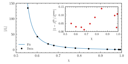
Figure 1: Absolute value of the critical coupling, $\beta_{\rm c}$, for spin-induced scalarization of a single BH as a function of the dimensionless spin $\chi$. We show the numerical data of Ref. [74] and the fitting formula (15). The inset shows the relative error between the fit and the data. We see that the error is less than $15\%$ in the range $0.5\leqslant\chi<1$ and less than $5\%$ for $\chi\lesssim 0.74$.

We use Eq. (14) as reference to choose the values of $\beta$ to probe scalarization of either one (or both) of the initial binary components or of the remnant BH.

Run	$d/M$	$\chi_{1}$	$\chi_{2}$	$\chi_{f}$	$\beta$	$\beta_{{\rm c},1}$	$\beta_{{\rm c},f}$	process
Setup A	$10$	$0$	$0$	$0.68$	$-14.30$	–	$-12.96$	$\bar{s}+\bar{s}\rightarrow s_{\uparrow}$
Setup B	$10$	$-0.6$	$-0.6$	$0.48$	$-11.00$	$-10.55$	–	$s_{\downarrow}+s_{\downarrow}\rightarrow\bar{s}_{\uparrow}$

Table 1: Setup of the simulations of equal-mass, quasi-circular BH binaries. We show the initial separation $d/M$, the initial dimensionless spins $\chi_{1}$ and $\chi_{2}$ of each binary component, the dimensionless spin $\chi_{f}$ of the remnant, and the dimensionless coupling constant $\beta$ used in the simulations. For reference, we also show the critical values to scalarize the initial ($\beta_{\rm c,1}=\beta_{\rm c,2}$) or final ($\beta_{{\rm c},f}$) BHs, calculated using Eqs. (14) and (15). The last column summarizes the process that unfolds during the simulation. We use $\bar{s}$ and $s$ to denote unscalarized and scalarized states, respectively, and the subscript $\uparrow$ ($\downarrow$) indicates spin aligned (anti-aligned) with the orbital angular momentum, which is assumed to be $\uparrow$. See Fig. 2 for additional details.

Here, we present two key simulations, listed in Table 1 and illustrated in Fig. 2, with the following setups:

1. in Table 1 is designed to address our first question: does the formation of a highly spinning remnant cause spin-induced dynamical scalarization? Here, we consider a binary of initially non-spinning, unscalarized BHs that merges into a spinning, scalarized remnant as illustrated in Fig. 2a. The BHs complete $10$ orbits prior to their merger at $t_{\rm M}=927M$, as estimated from the peak in the gravitational (quadrupole) waveform; see the bottom panel of Fig. 3. When the coupling $\beta$ is negative, the squared effective mass (5) of the initial BHs (with $\chi=0$) is positive definite everywhere outside their horizons, and so they are initially not scalarized. The final BH has a dimensionless spin of $\chi_{f}=0.68$ and mass $m_{f}\sim M$. For a BH with these parameters, the critical coupling is $\beta_{{\rm c},f}\approx\beta_{\rm c}(1,0.68)\approx-12.96$; cf. Eq. (14). In our simulation we chose $|\beta|>|\beta_{{\rm c},f}|$ such that the remnant BH is indeed scalarized. In this simulation, we initialize the scalar field according to Eq. (III.1) around each binary component. The scalar field disperses early in the simulation, leaving each BH unscalarized and a negligible, but nonvanishing ambient scalar field in the numerical grid. Notice that if we had set $\Phi|_{t=0}=0$, there would be no scalar field dynamics [see Eq. (3)].

2. in Table 1 is designed to address our second question: is the dynamical descalarization found in Ref. [45] a general phenomenon? Is there a spin-induced dynamical descalarization? Here we consider a binary of initially rotating, scalarized BHs with spins $\chi_{1}=\chi_{2}=-0.6$, anti-aligned with the orbital angular momentum as illustrated in Fig. 2b. Each of the components of the binary has a mass $m_{1}=m_{2}=M/2$. Inserting these parameters in Eq. (14), we find $\beta_{{\rm c},1}=\beta_{{\rm c},2}=\beta_{\rm c}(1/2,-0.6)\approx-10.55$. In our simulations, we set $|\beta|\gtrsim|\beta_{\rm c}(1/2,-0.6)|$ such that the initial BHs are scalarized. The initial BHs merge into a final rotating BH that has a spin aligned with the orbital angular momentum of the previously inspiralling system, with a spin magnitude $\chi_{f}=0.48$. This value is below the threshold for spin-induced scalarization, and so the remnant BH does not support scalar hair.

(a) Setup A

(b) Setup B

Figure 2: Binary BH simulations, where $s$ ($\bar{s}$) stands for initial or final BH states that are scalarized (unscalarized) and with spin along the positive ($\uparrow$) or negative ($\downarrow$) $z$-direction (i.e., aligned or anti-aligned with the orbital angular momentum, assuming the latter is $\uparrow$). BH states without an arrow are non-spinning. Panel 2a illustrates a process of spin-induced dynamical scalarization: two initially unscalarized BHs produce a spinning, scalarized remnant. Panel 2b illustrates a process of dynamical descalarization: two initially rotating, scalarized BHs whose spin is anti-aligned with the orbital angular momentum merge into a rotating BH with a smaller spin magnitude. Consequently, the remnant descalarizes.

To show that our qualitative results are robust for a large variety of BH spin parameters, we have performed a series of additional simulations listed in Table 2 of Appendix A. All simulations presented in Tables 1 and 2 have the same grid setup: the numerical domain was composed of a Cartesian box-in-box AMR grid structure with seven refinement levels. The outer boundary was located at $255.5M$. We use a grid spacing of $\textrm{d}x=0.7M$ on the outermost refinement level to ensure a sufficiently high resolution in the wave zone. The region around the BHs has a resolution of $\textrm{d}x=0.011M$. To validate our code and estimate the numerical error of our simulations, we performed convergence tests for our most demanding simulation with $\chi_{1,2}=-0.6$, corresponding to Setup B in Table 1. The relative error in the gravitational quadrupole waveform is $\Delta\Psi_{4,22}/\Psi_{4,22}\leqslant 0.8\%$, while the relative error of the scalar charge accumulates to $\Delta\Phi_{00}/\Phi_{00}\leqslant 30\%$ in the last orbits before merger; the latter is $\Delta\Phi_{00}/\Phi_{00}\leqslant 15\%$ in the merger and ringdown phase. The large error in the scalar field, close to the BHs merger, is a consequence of the exponential growth of the scalar field during inspiral. As our investigation is of a qualitative nature, this cumulative error is not a cause of concern for our results. However, a future quantitative analysis would have to address this issue. See Appendix B for details.

IV Results

IV.1 Spin-induced dynamical scalarization

Here we present key results obtained with simulation Setup A (see Sec. III.3), corresponding to Fig. 2a. In particular, we show that an initially unscalarized BH binary can indeed form a hairy, rotating remnant.

This process is illustrated in the top panel of Fig. 3, where we present the time evolution of the scalar field’s monopole charge, $r_{\rm ex}\Phi_{00}$, measured at $r_{\rm ex}=100M$, and shifted in time such that $(t-r_{\rm ex}-t_{\rm M})/M=0$ indicates the time of merger. The scalar field perturbation that is initially present in our simulations remains small during the entire inspiral. See, for instance, the amplitudes $r_{\rm ex}\Phi_{\ell m}$ at $(t-r_{\rm ex}-t_{\rm M})/M<0$ which are of ${\cal{O}}(10^{-4})$ or ${\cal{O}}(10^{-6})$. Yet, we see an exponential growth of the scalar charge, $r_{\rm ex}\Phi_{00}\sim e^{\omega_{\rm I,00}t}$, that exceeds the background fluctuations, approximately $100M$ after the merger. We estimate the growth rate (for our choice of $\beta$) to be $M\omega_{\rm I,00}\sim 0.062$ by fitting to the numerical data. We show this with the dotted red line in the top and middle panels.

We find a similar behavior in the scalar field quadrupole, as shown in the middle panel of Fig. 3. That is, both the axisymmetric $(\ell,m)=(2,0)$ and the $(\ell,m)=(2,2)$ multipoles are excited and grow exponentially with a rate of $M\omega_{\rm I}\sim 0.062$. For the form of the coupling function considered here, the rate appears to be independent of the $(\ell,m)$ multipole and is determined by the coupling constant $\beta$, as we further discuss later. The quadrupole scalar field is absent in the initial data because we initialized the scalar field with a spherically symmetric distribution around each of the BHs. Hence, the scalar field quadrupole we observe is caused by the “stirring” of the ambient scalar field due to the dynamical binary BH spacetime, which has a quadrupole moment. These $\Phi_{2m}$ multipoles also become unstable eventually, but at a later time relative to the monopole, as is evident by comparing the top and middle panels of Fig. 3. The exponential growth of the $\Phi_{2m}$ multipoles is consistent with the findings in Refs. [73, 77], showing that higher-$\ell$ and $m\neq 0$ scalar field multipoles can also become unstable.

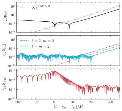
Figure 3: Evolution of the scalar field monopole (top panel), scalar field $\ell=2$ multipoles (middle panel) and the gravitational waveform of the background spacetime (bottom panel) for Setup A in Table 1. We rescale the multipoles by the extraction radius $r_{\rm ex}=100M$, and shift them in time such that $(t-r_{\rm ex}-t_{\rm M})/M=0$ indicates the time of merger, determined by the peak of the gravitational waveform.

All of these results beg for the following questions: at what stage in the binary’s evolution is the scalar field instability induced? Is it due to the orbital angular momentum at the late inspiral or is it due to the angular momentum of the remnant BH? As we discussed in Sec. II.2, a necessary (but not sufficient) condition for the tachyonic instability to occur is for the GB invariant to become negative outside the BH horizon in the $\beta<0$ case; see Eq. (8). To address these questions, we inspect the behavior of the GB invariant at different stages throughout the evolution.

In Fig. 4 we show a close-up of the GB invariant’s (top panel) and the scalar field’s (bottom panel) profiles along the $z$-axis, parallel to the orbital angular momentum, at different time snapshots throughout the evolution. In Fig. 5 we show the GB invariant $\mathscr{G}$ together with snapshots of the scalar field $\Phi$ in the $xz$-plane, perpendicular to the orbital plane of the binary. The snapshots correspond to time instants during the inspiral (top left), half an orbit before merger (top right), at the formation of the common apparent horizon (CAH) (bottom left) and about $200M$ after the merger (bottom right). The color map represents the scalar field amplitude and is shared among all panels, while the contours are isocurvature levels $|\mathscr{G}M^{4}|=\{1,\,10^{-1},\,10^{-2},\,10^{-3}\}$, with positive (negative) values of $\mathscr{G}$ in black (red). We also show the location of the individual BHs using their apparent horizons, represented as ellipses with center, semi-major and semi-minor axes given by the centroid, maximum and minimum radial directions as obtained with the AHFinderDirect thorn [110, 111]. We do not show the evolution of $\mathscr{G}$ in the equatorial plane because we did not observe negative regions forming on this plane throughout the entire simulation.

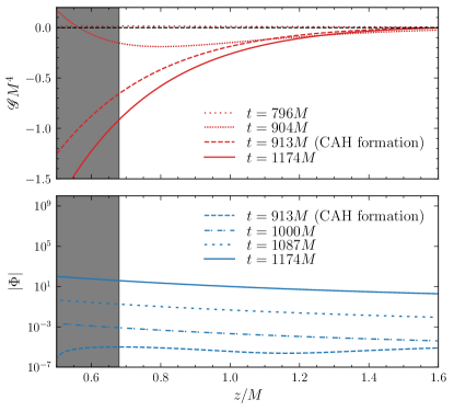
Figure 4: Profiles of the GB invariant (top panel) and of the scalar field (bottom panel), corresponding to Setup A in Table 1, along the $z$-axis in a close-up region near the CAH. The curves correspond to different times throughout the evolution. The shaded region indicates the CAH, shown $t=100M$ after its formation when the final BH has relaxed to its stationary state. The GB invariant becomes negative during the BHs’ last orbit before merger, and settles to its profile around the final rotating BH with dimensionless spin $\chi_{f}=0.68$. In response, the scalar field becomes unstable.

During the early inspiral, the GB invariant is positive around the individual, non-spinning BHs, and the scalar field remains small across the numerical grid as can be seen in the top left panel of Fig. 5. However, about half an orbit before merger, we see the formation of regions between the two BHs where the GB invariant is negative; see top right panel of Fig. 5 and top panel of Fig. 4, $t=904M$ curve. By the time $t=904M$, the effective mass squared defined in Eq. (8) has become negative and this, we re-emphasize, is a necessary, but not sufficient condition for the tachyonic instability to occur.

As the BHs merge and the system settles to a final, rotating BH, the GB invariant remains negative along the $z$-axis, which now coincides with the remnant BH’s rotation axis. This is illustrated in the bottom panels of Fig. 5, which correspond to the instant of the formation of the CAH (bottom left) and to about $200M$ after the merger (bottom right). In response, the scalar field grows exponentially as can be seen in its profiles shown in the bottom panel of Fig. 4 for different times after the CAH has formed. The scalar field assumes a predominantly dipolar spatial distribution along the BH’s spin axis, a consequence of the regions where the GB invariant is negative. We note that the scalar field continues to grow instead of settling to a stationary bound state because the magnitude of the coupling is larger than the critical value for spin-induced scalarization for the final BH with spin $\chi_{f}=0.68$; see Table 1.

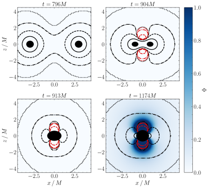
Figure 5: Snapshots of the scalar field, $\Phi$, and the GB invariant in the $xz$-plane corresponding to Setup A in Table 1. The color map indicates the amplitude of the scalar field. The isocurvature contours of the GB invariant correspond to $|\mathscr{G}M^{4}|=1$ (solid line), $|\mathscr{G}M^{4}|=10^{-1}$ (dashed line), $|\mathscr{G}M^{4}|=10^{-2}$ (dot-dashed line), $|\mathscr{G}M^{4}|=10^{-3}$ (dotted line), Black (red) lines correspond to positive (negative) values of $\mathscr{G}$. We show the inspiral (top left), half an orbit before merger (top right), formation of the first CAH (bottom left) and about $200M$ after the merger.

To verify that the regions of negative GB curvature before the merger can induce the instability, we repeated the simulation of Setup A with a smaller initial BH separation of $d=6M$ and a large-in-magnitude coupling constant $\beta=-10^{3}$; see Setup A1 in Table 2. Although this choice of coupling, with $|\beta|\gg|\beta_{{\rm c},f}|=|\beta_{\rm c}(1,0.68)|$, may appear unphysical it has the desired effect of being able to cause the instability before the merger and with a short time-scale; both effects are controlled by $|\beta|$. This can be seen in Fig. 6, where we show the evolution of the scalar field multipoles, and in Fig. 7, where we show the field’s profile along the rotation axis. Indeed, shortly after the GB invariant becomes negative, the scalar field grows exponentially and exceeds the magnitude of its background fluctuations at about $t=20M$ before the CAH is first found.

In summary, if $|\beta|$ is large enough, the BHs’ late inspiral and merger may be affected by the sGB scalar field. However, for $|\beta|$-values near the scalarization threshold, the inspiral and merger of initially unscalarized BH binaries, and their GW emission, are identical to that of GR and imprints of the sGB scalar field only appear during the late ringdown. Such effects may be very difficult (if not impossible) to detect, and this is what we refer to as stealth scalarization.

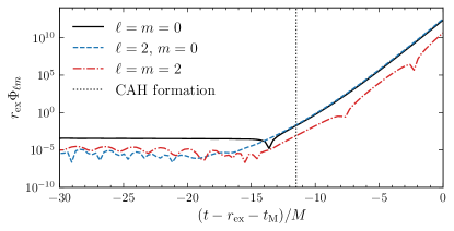
Figure 6: Evolution of the $\ell=m=0$ (solid line), $\ell=2$, $m=0$ (dashed line) and $\ell=m=2$ (dot-dashed line) scalar field multipoles for the coupling $\beta=-10^{3}$; cf. Setup A1 in Table 2. We rescale the multipoles by the extraction radius $r_{\rm ex}=50M$ and shift them such that $(t-r_{\rm ex}-t_{\rm M})/M=0$ indicates the time of merger determined by the peak in the gravitational waveform. For comparison we also show the formation of the CAH (dotted line). We observe that the scalar field grows exponentially about $20M$ prior to the merger.

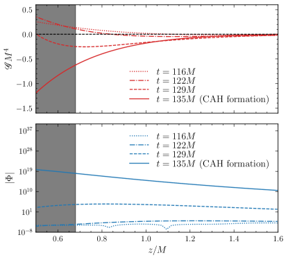
Figure 7: Same as Fig. 4, but for Setup A1 in Table 2. We see that the GB invariant (top panel) becomes negative and triggers the excitation of the scalar field (bottom panel) before the formation of the CAH, indicated by the gray region.

IV.2 Spin-induced dynamical descalarization

In this section we present our key results obtained with simulation Setup B in Table 2 (see Sec. III.3), illustrated in Fig. 2b. The setup corresponds to two initially rotating, scalarized BHs (whose spin is anti-aligned with the orbital angular momentum) that produce a unscalarized remnant with a spin magnitude below the scalarization threshold for any choice of the coupling constant.

In Fig. 8 we show snapshots of the scalar field and the GB invariant in the $xz$-plane, perpendicular to the binary’s orbital plane, during the inspiral (top left), half an orbit before the merger (top right), at the merger (bottom left) and about $t=100M$ after the merger (bottom right). We illustrate the location of the BHs by their apparent horizons. The color-coding represents the amplitude of the scalar field and is shared among all panels. The contours represent the isocurvature lines $|\mathscr{G}M^{4}|=\{1,\,10^{-1},\,10^{-2},\,10^{-3}\}$, with positive (negative) values shown in black (red). The spin magnitude of the two inspiraling BHs is sufficiently large to yield a GB invariant that has negative regions outside the BHs’ horizon. Combined with our choice of $|\beta|$, the BHs sustain a scalar field bound state, as shown in the top left panel of Fig. 8 and the BHs carry a scalar “charge” during the inspiral. As the BHs merge, they form a single, rotating BH which has a spin aligned with the orbital angular momentum and a magnitude of $\chi_{f}=0.48$. For this spin magnitude, the GB invariant is positive everywhere outside the BH’s horizon, as shown in the bottom row of Fig. 8. As a consequence, the effective mass-squared becomes positive everywhere in the BH’s exterior and the scalar field bound states are no longer supported. That is, the scalar field dissipates, and the BH dynamically descalarizes, in agreement with the no-hair theorem of Ref. [69].

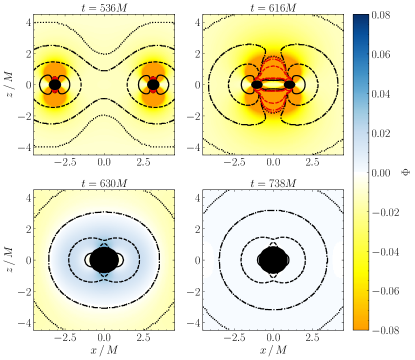
Figure 8: Snapshots of the scalar field, $\Phi$, and the GB invariant, $\mathscr{G}$, in the $xz$-plane, corresponding to Setup B in Table 2. The color map represents the amplitude of the scalar field. The isocurvature contours indicate the magnitude of the GB invariant with $|\mathscr{G}M^{4}|=1$ (solid line), $|\mathscr{G}M^{4}|=10^{-1}$ (dashed line), $|\mathscr{G}M^{4}|=10^{-2}$ (dot-dashed line), $|\mathscr{G}M^{4}|=10^{-3}$ (dotted line), with positive (negative) values shown in black (red). We show the inspiral (top left), half an orbit before merger (top right), $10M$ after the CAH formation (bottom left) and about $100M$ after the merger (bottom right).

These phenomena can also be seen in Fig. 9, where we show the profiles of the GB invariant (top panel) and of the scalar field (bottom panel) along the $z$-axis (parallel to orbital angular momentum) for several instants during the evolution. The shaded region indicates the apparent horizon of the final BH. The GB invariant remains negative outside the individual BHs during their (late) inspiral. Only when the CAH first forms, does the GB invariant become positive everywhere outside the remnant BH’s horizon At this point, the effective mass-squared becomes positive, the tachyonic instability that kept each BH scalarized switches off, and the scalar field dissipates as shown in the bottom panel of Fig. 9.

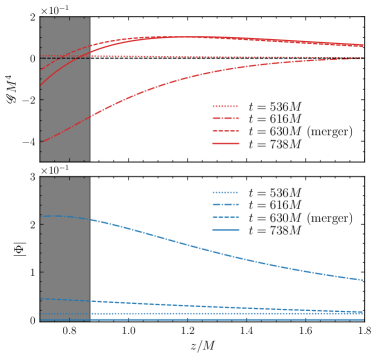
Figure 9: Profiles of the GB invariant (top panel) and of the scalar field (bottom panel) for Setup B in Table 2 along the $z$-axis. The lines correspond to different times during the evolution. The shaded region indicates the CAH, shown $100M$ after its formation. The GB invariant becomes positive outside the horizon when the CAH is first formed. Consequently, the scalar field magnitude decreases and the remnant BH descalarizes.

Does the presence of scalar charges during the inspiral produce scalar radiation? The answer is affirmative as can be seen in Fig. 10 where we show the time evolution of the scalar field monopole (top panel) and quadrupole (middle panel). For comparison, we also display the gravitational quadrupole waveform of the background spacetime (bottom panel). The scalar field monopole quantifies the development of the combined scalar charge of the BH binary measured on spheres of radius $r_{\rm ex}=100M$, i.e., enclosing the entire binary. The total scalar charge remains approximately constant during the inspiral as the coupling is close to its critical value. Its magnitude increases about $10M$ before the merger which coincides with the formation of a joined region in which the GB invariant is negative due to the proximity of the two BHs As the BHs merge into a single rotating remnant with a spin below the threshold for the spin-induced scalarization, the scalar charge decays as illustrated in the inset of Fig. 10 (top panel). Because the scalar charges anchored around each BH follow the holes’ orbital motion, they generate scalar radiation. In general, one would expect the scalar dipole to dominate the signal, as is also the case for shift-symmetric sGB gravity [41, 37, 38]. In the simulations shown here, however, the scalar dipole is suppressed due to the symmetry of the system (equal mass and spin of the companions), and the $\ell=m=2$ multipole dominates.

The scalar waveform is displayed in the middle panel of Fig. 10 and shows the familiar chirp pattern: its amplitude and frequency increase as the scalar charges inspiral (following the inspiraling BHs in the background), and culminates in a peak as the BHs merge. The phase of the scalar field quadrupole clearly tracks its gravitational counterpart. Therefore, we deduce that the morphology (phase evolution) of the observed scalar quadrupole radiation is a result of the orbital dynamics of the system. A sufficiently large magnitude of the coupling constant may lead to an additional scalarization of the $\ell=2$ mode, which would become manifest as an exponential growth of the signal superposed with the chirp. This situation is analogous to the evolutions with positive coupling shown in our previous work [45].

After the merger, the scalar quadrupole exhibits a quasi-normal ringdown pattern, i.e., an exponentially damped sinusoid, shown in the inset of Fig. 10 (middle panel). Here, in contrast to Ref. [45], descalarization occurs due to the vanishing of negative GB regions outside the remnant BH (because its final spin is $|\chi_{f}|<0.5$), rather than due to a reduction of positive curvature (because of an increase in mass). We note that the scalar field rings down on similar timescales as the GW signal shown in the bottom panel of Fig. 10 for comparison. Therefore, one might expect a modification to the GW ringdown if backreaction onto the spacetime is included.

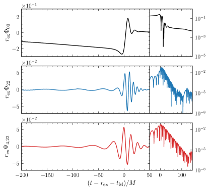
Figure 10: Evolution of the scalar field monopole (top panel) and quadrupole (middle panel) and gravitational quadrupole (bottom panel) for Setup B in Table 1. The waveforms are rescaled by the extractions radius $r_{\rm ex}=100M$ and shifted in time such that $(t-r_{\rm ex}-t_{\rm M})/M=0$ at the merger. In the insets we show the absolute values of the multipoles, in logarithmic scale, during the merger and ringdown.

V Discussion

In this paper, we continued our study of dynamical scalarization and descalarization in binary BH mergers in sGB gravity by extending our previous work [45]. The latter focused on a positive coupling constant between the scalar field and the GB invariant, yielding dynamical descalarization in binary BH mergers. As a natural continuation, here we studied a negative coupling for which the BHs’ spins play a major role in determining the onset of scalarization. In particular, we have shown that the merger remnant can either dynamically scalarize or dynamically descalarize depending on its spin and mass.

Spin-induced dynamical scalarization occurs when the merger remnant grows a scalar charge during coalescence due to the large spin of the remnant. In cases like this, the initial binary components lack a charge because their spins are not large enough to support one [73, 76, 74, 75, 77, 78]. However, after the objects merge, the remnant BH spins faster than either component, allowing for a charge to grow. We found that it is possible for the scalar charge to grow as early as 1–2 orbits before a CAH has formed if the coupling $|\beta|$ is extremely large. This occurs because there are spacetime regions before merger (and near the poles of the future remnant) with a negative GB invariant, and a sufficient large value of $|\beta|$ allows bound states to form fast enough. We also found that if the coupling $|\beta|$ is close to the threshold, then scalarization occurs only in the late ringdown, because of the timescale required for the bound states to form.

Is such spin-induced scalarization detectable with current or future GW observatories? For values of $|\beta|$ near the scalarization threshold the instability timescale is large and the effects of the scalar field growth would only appear at times much later than the merger and, more importantly, after the start of the ringdown. Hence, the inspiral-merger-ringdown of such a binary would be indistinguishable from one in GR, and scalarization would be a hidden or “stealth” effect, i.e., the remnant BH would acquire a charge, but its formation would not lead to an easily measurable effect. For instance, during the GW ringdown, which is dominated by the fundamental $(\ell,m)=(2,2)$ quasinormal mode (QNM) frequency, we know that at a spin of $\chi\approx 0.68$, the decay time is approximately $\tau\approx 12.3M$ [117]. Hence, after $100M$ from the peak in the waveform, the dominant mode has decayed by roughly $\exp(-t/\tau)\approx\exp(-100/12.3)\approx 10^{-4}$. If the dominant QNM frequency begins to be modified only after $100M$, the GW has decayed so much that detecting this change or constraining it would be essentially impossible.

Is there no hope to detect such late times scalarization? Not necessarily. If we were to include the scalar field backreaction onto the spacetime, one could entertain the possibility that the late time growth of the scalar field (in particular of $\Phi_{22}$) and the subsequent readjustment of the spinning remnant BH to its scalarized counterpart could result in a second GW signal. Confirming this possibility and, if confirmed, characterizing such a GW signal is left for future work.

Spin-induced dynamical descalarization occurs when the merger remnant loses its scalar charge during coalescence due to the low spin of the remnant. In cases like this, the initial binary components are spinning fast enough that each of them has a scalar charge and the remnant descalarizes if it has spin $\chi_{f}\leqslant 0.5$. Here we demonstrated this effect in a example in which the initial binary components have their spin angular momenta anti-aligned with the orbital angular momentum. The merger produces a remnant BH with $\chi_{f}=0.48$, for which no scalar field bound states are supported and the field is radiated away shortly ($\sim 10M$) after the CAH formation.

Is such spin-induced descalarization detectable with current or future GW observatories? For such descalarization to be detectable, one must first detect that the binary components were scalarized during the inspiral. Our simulations showed that the scalar charges lead to scalar quadrupole radiation because of the highly symmetric configurations (equal mass, equal spin magnitude) we chose to evolve. More realistic astrophysical configurations (with unequal masses and unequal spin magnitudes) forces the binary to emit scalar dipole radiation. Such emission of dipole or quadrupole radiation accelerates the inspiral, and thus affect the GW phase at $-$1PN and 0PN respectively, as shown in shift-symmetric theories [34, 35, 36, 37, 38, 39]. These effects in the inspiral are observable and can thus be constrained with current ground-based [8, 22, 23, 24, 25] and future detectors [118, 119] within the parameterized post-Einsteinian framework [120, 121, 122, 123], provided the binary is of sufficiently low mass such that enough of the inspiral is observed [119]. In fact, a constraint of this type was recently obtained using the GW190814 event [124] in [21].

Let us then assume, for the sake of argument, that some future event reveals a scalar charge in the inspiraling binary components. Our results then indicate that descalarization may be detectable, if there is enough signal-to-noise ratio in the merger and ringdown [41, 42]. This is because this process occurs at the same time and with the same timescales as the GW merger and ringdown, see Fig. 10. Future work could study the backreaction of the scalar field onto the metric to determine the magnitude of these modifications in the transient phase, without which one cannot assess detectability confidently. Our results indicate that descalarization might be best probed with a full inspiral-merger-ringdown analysis of the GW signal.

Appendix A Full suite of simulations

Setup	$d/M$	$\chi_{1}$	$\chi_{2}$	$\chi_{f}$	$\beta$	$\beta_{{\rm c},1}$	$\beta_{{\rm c},f}$	process
A	$10$	$0$	$0$	$0.68$	$-14.30$	–	$-12.96$	$\bar{s}+\bar{s}\rightarrow s_{\uparrow}$
A1	$6$	$0$	$0$	$0.68$	$-1000$	–	$-12.96$	$\bar{s}+\bar{s}\rightarrow s_{\uparrow}$
A2	$10$	$0.6$	$0.6$	$0.85$	$-2.9$	$-10.55$	$-3.01$	$\bar{s}_{\uparrow}+\bar{s}_{\uparrow}\rightarrow s_{\uparrow}$
A3	$10$	$0.6$	$0.6$	$0.85$	$-12.0$	$-10.55$	$-3.01$	$s_{\uparrow}+s_{\uparrow}\rightarrow s_{\uparrow}$
A4	$10$	$0.0$	$0.6$	$0.77$	$-12.0$	$-10.55$	$-5.59$	$\bar{s}+s_{\uparrow}\rightarrow s_{\uparrow}$
B	$10$	$-0.6$	$-0.6$	$0.48$	$-11.50$	$-10.55$	–	$s_{\downarrow}+s_{\downarrow}\rightarrow\bar{s}_{\uparrow}$
B2	$10$	$0.4$	$-0.6$	$0.64$	$-12.0$	$-10.55$	$-21.50$	$\bar{s}_{\uparrow}+s_{\downarrow}\rightarrow\bar{s}_{\uparrow}$

Table 2: List of our complete series of simulations. We denote the initial separation $d/M$ with $M$ being the total mass, $\chi_{1}$ and $\chi_{2}$ are the initial dimensionless spin parameters of each BH, and $\chi_{f}$ is the final dimensionless spin parameter of the remnant. We use $\bar{s}$ and $s$ to denote unscalarized and scalarized states, respectively, and the subscript $\uparrow$ ($\downarrow$) indicates spin aligned (anti-aligned) with the orbital angular momentum. The coupling chosen for each simulation is given by $\beta$, whereas $\beta_{{\rm c},1}$ and $\beta_{{\rm c},f}$ denote the critical couplings for the component/remnant BHs respectively.

We ran a larger series of simulations, listed in Table 2, of equal-mass BH binaries with varying initial spin that show a qualitatively same behaviour as the runs presented in the main text. In particular, we simulated a series of initially spinning, unscalarized black holes that formed a scalarized remnant with larger spin. We also list example simulations in which one or both initial BHs are scalarized and they merge into an unscalarized remnant.

Appendix B Validation tests

To validate our code, we performed a suite of convergence tests. We ran Setup B, our numerically most demanding setup, at a lower resolution of $\textrm{d}x_{\rm low}=0.8M$ and a higher resolution of $\textrm{d}x_{\rm high}=0.625M$. The runs in the main text use a medium resolution of $\textrm{d}x_{\rm med}=0.7M$. The grid setup is the same across all simulations, see Sec. III. We estimated the order of convergence $n$ and its associated convergence factor $Q_{n}$,

$$Q_{n}=\frac{\left(\textrm{d}x_{\rm low}\right)^{n}-\left(\textrm{d}x_{\rm med}\right)^{n}}{\left(\textrm{d}x_{\rm med}\right)^{n}-\left(\textrm{d}x_{\rm high}\right)^{n}}\,.$$ (16)

Figure 11: Convergence plots for the $\ell=m=2$ mode of the gravitational waveform (left panel) and the $\ell=m=0$ mode of the scalar field (right panel). In both panels, we show the difference between the low and medium resolution run (solid line) and the medium and high resolution run (dashed line). The latter is rescaled by $Q_{4}=1.94$, indicating fourth order convergence. The lines are shifted in time such that $(t-r_{\rm ex}-t_{\rm M})/M=0$ indicates the time of merger and they are rescaled by the extraction radius $r_{\rm ex}=100M$.

We computed the $n$ and $Q_{n}$ for the gravitational waveform, $\Psi_{4,22}$, of the background spacetime and for the scalar charge. We show the corresponding convergence plots in Fig. 11. For $\Psi_{4,22}$ we find fourth order convergence, and we estimate the numerical (truncation) error to be $\Psi_{4,22}/\Psi_{4,22}\leqslant 0.8\%$. For the scalar field charge, $\Phi_{00}$, we also find fourth order convergence. performed a convergence test on its $\ell=m=0$ multipole. We show our result in the right panel of Fig. 11.

We find a cumulative error $\Delta\Phi_{00}/\Phi_{00}\leqslant 30\%$ in the late inspiral. The numerical error in the merger and ringdown is $\Delta\Phi_{00}/\Phi_{00}\leqslant 15\%$. As we restrict this work to a qualitative analysis, this error does not affect the main results of the paper. Further quantitative work, such as forecasting constraints on the theory would require this issue to be addressed.

Finally, in Fig. 12, we show the Hamiltonian constraint $\mathcal{H}$ along the $z$-axis for Setup B at different time instants. The constraint violation remains below $10^{-5}$ outside the BH horizon through the simulation.

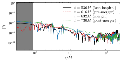
Figure 12: Hamiltonian constraint along the z-axis during the late-inspiral (solid black), half an orbit before merger (dashed red), at the time of merger from the peak of the gravitational waveform (dash-dot blue) and $100M$ after merger (dotted green). The shaded region indicates the CAH, shown $100M$ after merger.

References

- Abbott et al. [2019a] B. Abbott et al. (LIGO Scientific, Virgo), GWTC-1: A Gravitational-Wave Transient Catalog of Compact Binary Mergers Observed by LIGO and Virgo during the First and Second Observing Runs, Phys. Rev. X 9, 031040 (2019a), arXiv:1811.12907 [astro-ph.HE] .
- Abbott et al. [2021a] R. Abbott et al. (LIGO Scientific, Virgo), GWTC-2: Compact Binary Coalescences Observed by LIGO and Virgo During the First Half of the Third Observing Run, Phys. Rev. X 11, 021053 (2021a), arXiv:2010.14527 [gr-qc] .
- Abbott et al. [2021b] R. Abbott et al. (LIGO Scientific, VIRGO, KAGRA), GWTC-3: Compact Binary Coalescences Observed by LIGO and Virgo During the Second Part of the Third Observing Run (2021b), arXiv:2111.03606 [gr-qc] .
- Yunes and Siemens [2013] N. Yunes and X. Siemens, Gravitational-Wave Tests of General Relativity with Ground-Based Detectors and Pulsar Timing-Arrays, Living Rev. Rel. 16, 9 (2013), arXiv:1304.3473 [gr-qc] .
- Berti et al. [2015] E. Berti et al., Testing General Relativity with Present and Future Astrophysical Observations, Class. Quant. Grav. 32, 243001 (2015), arXiv:1501.07274 [gr-qc] .
- Berti et al. [2018a] E. Berti, K. Yagi, and N. Yunes, Extreme Gravity Tests with Gravitational Waves from Compact Binary Coalescences: (I) Inspiral-Merger, Gen. Rel. Grav. 50, 46 (2018a), arXiv:1801.03208 [gr-qc] .
- Berti et al. [2018b] E. Berti, K. Yagi, H. Yang, and N. Yunes, Extreme Gravity Tests with Gravitational Waves from Compact Binary Coalescences: (II) Ringdown, Gen. Rel. Grav. 50, 49 (2018b), arXiv:1801.03587 [gr-qc] .
- Yunes et al. [2016] N. Yunes, K. Yagi, and F. Pretorius, Theoretical Physics Implications of the Binary Black-Hole Mergers GW150914 and GW151226, Phys. Rev. D 94, 084002 (2016), arXiv:1603.08955 [gr-qc] .
- Abbott et al. [2016] B. P. Abbott et al. (LIGO Scientific, Virgo), Tests of general relativity with GW150914, Phys. Rev. Lett. 116, 221101 (2016), [Erratum: Phys.Rev.Lett. 121, 129902 (2018)], arXiv:1602.03841 [gr-qc] .
- Abbott et al. [2019b] B. P. Abbott et al. (LIGO Scientific, Virgo), Tests of General Relativity with GW170817, Phys. Rev. Lett. 123, 011102 (2019b), arXiv:1811.00364 [gr-qc] .
- Abbott et al. [2019c] B. Abbott et al. (LIGO Scientific, Virgo), Tests of General Relativity with the Binary Black Hole Signals from the LIGO-Virgo Catalog GWTC-1, Phys. Rev. D 100, 104036 (2019c), arXiv:1903.04467 [gr-qc] .
- Cardenas-Avendano et al. [2020] A. Cardenas-Avendano, S. Nampalliwar, and N. Yunes, Gravitational-wave versus X-ray tests of strong-field gravity, Class. Quant. Grav. 37, 135008 (2020), arXiv:1912.08062 [gr-qc] .
- Abbott et al. [2021c] R. Abbott et al. (LIGO Scientific, Virgo), Tests of general relativity with binary black holes from the second LIGO-Virgo gravitational-wave transient catalog, Phys. Rev. D 103, 122002 (2021c), arXiv:2010.14529 [gr-qc] .
- Silva et al. [2021a] H. O. Silva, A. M. Holgado, A. Cárdenas-Avendaño, and N. Yunes, Astrophysical and theoretical physics implications from multimessenger neutron star observations, Phys. Rev. Lett. 126, 181101 (2021a), arXiv:2004.01253 [gr-qc] .
- Abbott et al. [2021d] R. Abbott et al. (LIGO Scientific, VIRGO, KAGRA), Tests of General Relativity with GWTC-3 (2021d), arXiv:2112.06861 [gr-qc] .
- Ghosh et al. [2021] A. Ghosh, R. Brito, and A. Buonanno, Constraints on quasinormal-mode frequencies with LIGO-Virgo binary–black-hole observations, Phys. Rev. D 103, 124041 (2021), arXiv:2104.01906 [gr-qc] .
- Carullo [2021] G. Carullo, Enhancing modified gravity detection from gravitational-wave observations using the parametrized ringdown spin expansion coeffcients formalism, Phys. Rev. D 103, 124043 (2021), arXiv:2102.05939 [gr-qc] .
- Sennett et al. [2020] N. Sennett, R. Brito, A. Buonanno, V. Gorbenko, and L. Senatore, Gravitational-Wave Constraints on an Effective Field-Theory Extension of General Relativity, Phys. Rev. D 102, 044056 (2020), arXiv:1912.09917 [gr-qc] .
- Mehta et al. [2022] A. K. Mehta, A. Buonanno, R. Cotesta, A. Ghosh, N. Sennett, and J. Steinhoff, Tests of General Relativity with Gravitational-Wave Observations using a Flexible-Theory-Independent Method (2022), arXiv:2203.13937 [gr-qc] .
- Zhao et al. [2019] J. Zhao, L. Shao, Z. Cao, and B.-Q. Ma, Reduced-order surrogate models for scalar-tensor gravity in the strong field regime and applications to binary pulsars and GW170817, Phys. Rev. D 100, 064034 (2019), arXiv:1907.00780 [gr-qc] .
- Wong et al. [2022] L. K. Wong, C. A. R. Herdeiro, and E. Radu, Constraining spontaneous black hole scalarization in scalar-tensor-Gauss-Bonnet theories with current gravitational-wave data (2022), arXiv:2204.09038 [gr-qc] .
- Nair et al. [2019] R. Nair, S. Perkins, H. O. Silva, and N. Yunes, Fundamental Physics Implications for Higher-Curvature Theories from Binary Black Hole Signals in the LIGO-Virgo Catalog GWTC-1, Phys. Rev. Lett. 123, 191101 (2019), arXiv:1905.00870 [gr-qc] .
- Yamada et al. [2019] K. Yamada, T. Narikawa, and T. Tanaka, Testing massive-field modifications of gravity via gravitational waves, PTEP 2019, 103E01 (2019), arXiv:1905.11859 [gr-qc] .
- Perkins et al. [2021a] S. E. Perkins, R. Nair, H. O. Silva, and N. Yunes, Improved gravitational-wave constraints on higher-order curvature theories of gravity, Phys. Rev. D 104, 024060 (2021a), arXiv:2104.11189 [gr-qc] .
- Lyu et al. [2022] Z. Lyu, N. Jiang, and K. Yagi, Constraints on Einstein-dilation-Gauss-Bonnet gravity from black hole-neutron star gravitational wave events, Phys. Rev. D 105, 064001 (2022), arXiv:2201.02543 [gr-qc] .
- Silva et al. [2022] H. O. Silva, A. Ghosh, and A. Buonanno, Black-hole ringdown as a probe of higher-curvature gravity theories (2022), arXiv:2205.05132 [gr-qc] .
- Yagi et al. [2016] K. Yagi, L. C. Stein, and N. Yunes, Challenging the Presence of Scalar Charge and Dipolar Radiation in Binary Pulsars, Phys. Rev. D 93, 024010 (2016), arXiv:1510.02152 [gr-qc] .
- Metsaev and Tseytlin [1987] R. Metsaev and A. A. Tseytlin, Order (Two Loop) Equivalence of the String Equations of Motion and the Sigma Model Weyl Invariance Conditions: Dependence on the Dilaton and the Antisymmetric Tensor, Nucl. Phys. B 293, 385 (1987).
- Kanti and Tamvakis [1995] P. Kanti and K. Tamvakis, Classical moduli O() hair, Phys. Rev. D 52, 3506 (1995), arXiv:hep-th/9504031 .
- Cano and Ruipérez [2022] P. A. Cano and A. Ruipérez, String gravity in , Phys. Rev. D 105, 044022 (2022), arXiv:2111.04750 [hep-th] .
- Charmousis [2015] C. Charmousis, From Lovelock to Horndeski‘s Generalized Scalar Tensor Theory, Lect. Notes Phys. 892, 25 (2015), arXiv:1405.1612 [gr-qc] .
- Kobayashi et al. [2011] T. Kobayashi, M. Yamaguchi, and J. Yokoyama, Generalized G-inflation: Inflation with the most general second-order field equations, Prog. Theor. Phys. 126, 511 (2011), arXiv:1105.5723 [hep-th] .
- Kobayashi [2019] T. Kobayashi, Horndeski theory and beyond: a review, Rept. Prog. Phys. 82, 086901 (2019), arXiv:1901.07183 [gr-qc] .
- Yagi et al. [2012a] K. Yagi, L. C. Stein, N. Yunes, and T. Tanaka, Post-Newtonian, Quasi-Circular Binary Inspirals in Quadratic Modified Gravity, Phys. Rev. D 85, 064022 (2012a), [Erratum: Phys.Rev.D 93, 029902 (2016)], arXiv:1110.5950 [gr-qc] .
- Yagi et al. [2012b] K. Yagi, N. Yunes, and T. Tanaka, Gravitational Waves from Quasi-Circular Black Hole Binaries in Dynamical Chern-Simons Gravity, Phys. Rev. Lett. 109, 251105 (2012b), [Erratum: Phys.Rev.Lett. 116, 169902 (2016), Erratum: Phys.Rev.Lett. 124, 029901 (2020)], arXiv:1208.5102 [gr-qc] .
- Yagi et al. [2013] K. Yagi, L. C. Stein, N. Yunes, and T. Tanaka, Isolated and Binary Neutron Stars in Dynamical Chern-Simons Gravity, Phys. Rev. D 87, 084058 (2013), [Erratum: Phys.Rev.D 93, 089909 (2016)], arXiv:1302.1918 [gr-qc] .
- Shiralilou et al. [2021] B. Shiralilou, T. Hinderer, S. Nissanke, N. Ortiz, and H. Witek, Nonlinear curvature effects in gravitational waves from inspiralling black hole binaries, Phys. Rev. D 103, L121503 (2021), arXiv:2012.09162 [gr-qc] .
- Shiralilou et al. [2022] B. Shiralilou, T. Hinderer, S. M. Nissanke, N. Ortiz, and H. Witek, Post-Newtonian gravitational and scalar waves in scalar-Gauss–Bonnet gravity, Class. Quant. Grav. 39, 035002 (2022), arXiv:2105.13972 [gr-qc] .
- Julié and Berti [2019] F.-L. Julié and E. Berti, Post-Newtonian dynamics and black hole thermodynamics in Einstein-scalar-Gauss-Bonnet gravity, Phys. Rev. D 100, 104061 (2019), arXiv:1909.05258 [gr-qc] .
- Julié et al. [2022] F.-L. Julié, H. O. Silva, E. Berti, and N. Yunes, Black hole sensitivities in Einstein-scalar-Gauss-Bonnet gravity (2022), arXiv:2202.01329 [gr-qc] .
- Witek et al. [2019] H. Witek, L. Gualtieri, P. Pani, and T. P. Sotiriou, Black holes and binary mergers in scalar Gauss-Bonnet gravity: scalar field dynamics, Phys. Rev. D 99, 064035 (2019), arXiv:1810.05177 [gr-qc] .
- Okounkova [2020] M. Okounkova, Numerical relativity simulation of GW150914 in Einstein dilaton Gauss-Bonnet gravity, Phys. Rev. D 102, 084046 (2020), arXiv:2001.03571 [gr-qc] .
- East and Ripley [2021a] W. E. East and J. L. Ripley, Evolution of Einstein-scalar-Gauss-Bonnet gravity using a modified harmonic formulation, Phys. Rev. D 103, 044040 (2021a), arXiv:2011.03547 [gr-qc] .
- East and Ripley [2021b] W. E. East and J. L. Ripley, Dynamics of Spontaneous Black Hole Scalarization and Mergers in Einstein-Scalar-Gauss-Bonnet Gravity, Phys. Rev. Lett. 127, 101102 (2021b), arXiv:2105.08571 [gr-qc] .
- Silva et al. [2021b] H. O. Silva, H. Witek, M. Elley, and N. Yunes, Dynamical Descalarization in Binary Black Hole Mergers, Phys. Rev. Lett. 127, 031101 (2021b), arXiv:2012.10436 [gr-qc] .
- Doneva et al. [2022] D. D. Doneva, A. Vañó Viñuales, and S. S. Yazadjiev, Dynamical descalarization with a jump during black hole merger (2022), arXiv:2204.05333 [gr-qc] .
- Pani and Cardoso [2009] P. Pani and V. Cardoso, Are black holes in alternative theories serious astrophysical candidates? The Case for Einstein-Dilaton-Gauss-Bonnet black holes, Phys. Rev. D 79, 084031 (2009), arXiv:0902.1569 [gr-qc] .
- Blázquez-Salcedo et al. [2016] J. L. Blázquez-Salcedo, C. F. B. Macedo, V. Cardoso, V. Ferrari, L. Gualtieri, F. S. Khoo, J. Kunz, and P. Pani, Perturbed black holes in Einstein-dilaton-Gauss-Bonnet gravity: Stability, ringdown, and gravitational-wave emission, Phys. Rev. D 94, 104024 (2016), arXiv:1609.01286 [gr-qc] .
- Blázquez-Salcedo et al. [2020a] J. L. Blázquez-Salcedo, D. D. Doneva, S. Kahlen, J. Kunz, P. Nedkova, and S. S. Yazadjiev, Axial perturbations of the scalarized Einstein-Gauss-Bonnet black holes, Phys. Rev. D 101, 104006 (2020a), arXiv:2003.02862 [gr-qc] .
- Blázquez-Salcedo et al. [2020b] J. L. Blázquez-Salcedo, D. D. Doneva, S. Kahlen, J. Kunz, P. Nedkova, and S. S. Yazadjiev, Polar quasinormal modes of the scalarized Einstein-Gauss-Bonnet black holes, Phys. Rev. D 102, 024086 (2020b), arXiv:2006.06006 [gr-qc] .
- Pierini and Gualtieri [2021] L. Pierini and L. Gualtieri, Quasi-normal modes of rotating black holes in Einstein-dilaton Gauss-Bonnet gravity: the first order in rotation, Phys. Rev. D 103, 124017 (2021), arXiv:2103.09870 [gr-qc] .
- Bryant et al. [2021] A. Bryant, H. O. Silva, K. Yagi, and K. Glampedakis, Eikonal quasinormal modes of black holes beyond general relativity. III. Scalar Gauss-Bonnet gravity, Phys. Rev. D 104, 044051 (2021), arXiv:2106.09657 [gr-qc] .
- Campbell et al. [1992] B. A. Campbell, N. Kaloper, and K. A. Olive, Classical hair for Kerr-Newman black holes in string gravity, Phys. Lett. B 285, 199 (1992).
- Mignemi and Stewart [1993] S. Mignemi and N. Stewart, Charged black holes in effective string theory, Phys. Rev. D 47, 5259 (1993), arXiv:hep-th/9212146 .
- Kanti et al. [1996] P. Kanti, N. Mavromatos, J. Rizos, K. Tamvakis, and E. Winstanley, Dilatonic black holes in higher curvature string gravity, Phys. Rev. D 54, 5049 (1996), arXiv:hep-th/9511071 .
- Torii et al. [1997] T. Torii, H. Yajima, and K.-i. Maeda, Dilatonic black holes with Gauss-Bonnet term, Phys. Rev. D 55, 739 (1997), arXiv:gr-qc/9606034 .
- Guo et al. [2008] Z.-K. Guo, N. Ohta, and T. Torii, Black Holes in the Dilatonic Einstein-Gauss-Bonnet Theory in Various Dimensions. I. Asymptotically Flat Black Holes, Prog. Theor. Phys. 120, 581 (2008), arXiv:0806.2481 [gr-qc] .
- Yunes and Stein [2011] N. Yunes and L. C. Stein, Non-Spinning Black Holes in Alternative Theories of Gravity, Phys. Rev. D 83, 104002 (2011), arXiv:1101.2921 [gr-qc] .
- Sotiriou and Zhou [2014a] T. P. Sotiriou and S.-Y. Zhou, Black hole hair in generalized scalar-tensor gravity, Phys. Rev. Lett. 112, 251102 (2014a), arXiv:1312.3622 [gr-qc] .
- Sotiriou and Zhou [2014b] T. P. Sotiriou and S.-Y. Zhou, Black hole hair in generalized scalar-tensor gravity: An explicit example, Phys. Rev. D 90, 124063 (2014b), arXiv:1408.1698 [gr-qc] .
- Benkel et al. [2016] R. Benkel, T. P. Sotiriou, and H. Witek, Dynamical scalar hair formation around a Schwarzschild black hole, Phys. Rev. D 94, 121503 (2016), arXiv:1612.08184 [gr-qc] .
- Benkel et al. [2017] R. Benkel, T. P. Sotiriou, and H. Witek, Black hole hair formation in shift-symmetric generalised scalar-tensor gravity, Class. Quant. Grav. 34, 064001 (2017), arXiv:1610.09168 [gr-qc] .
- Antoniou et al. [2018a] G. Antoniou, A. Bakopoulos, and P. Kanti, Evasion of No-Hair Theorems and Novel Black-Hole Solutions in Gauss-Bonnet Theories, Phys. Rev. Lett. 120, 131102 (2018a), arXiv:1711.03390 [hep-th] .
- Antoniou et al. [2018b] G. Antoniou, A. Bakopoulos, and P. Kanti, Black-Hole Solutions with Scalar Hair in Einstein-Scalar-Gauss-Bonnet Theories, Phys. Rev. D 97, 084037 (2018b), arXiv:1711.07431 [hep-th] .
- Prabhu and Stein [2018] K. Prabhu and L. C. Stein, Black hole scalar charge from a topological horizon integral in Einstein-dilaton-Gauss-Bonnet gravity, Phys. Rev. D 98, 021503 (2018), arXiv:1805.02668 [gr-qc] .
- Saravani and Sotiriou [2019] M. Saravani and T. P. Sotiriou, Classification of shift-symmetric Horndeski theories and hairy black holes, Phys. Rev. D 99, 124004 (2019), arXiv:1903.02055 [gr-qc] .
- R. et al. [2022] A. H. K. R., E. R. Most, J. Noronha, H. Witek, and N. Yunes, How do spherical black holes grow monopole hair?, Phys. Rev. D 105, 064041 (2022), arXiv:2201.05178 [gr-qc] .
- Doneva and Yazadjiev [2018] D. D. Doneva and S. S. Yazadjiev, New Gauss-Bonnet Black Holes with Curvature-Induced Scalarization in Extended Scalar-Tensor Theories, Phys. Rev. Lett. 120, 131103 (2018), arXiv:1711.01187 [gr-qc] .
- Silva et al. [2018] H. O. Silva, J. Sakstein, L. Gualtieri, T. P. Sotiriou, and E. Berti, Spontaneous scalarization of black holes and compact stars from a Gauss-Bonnet coupling, Phys. Rev. Lett. 120, 131104 (2018), arXiv:1711.02080 [gr-qc] .
- Macedo et al. [2019] C. F. Macedo, J. Sakstein, E. Berti, L. Gualtieri, H. O. Silva, and T. P. Sotiriou, Self-interactions and Spontaneous Black Hole Scalarization, Phys. Rev. D 99, 104041 (2019), arXiv:1903.06784 [gr-qc] .
- Cunha et al. [2019] P. V. Cunha, C. A. Herdeiro, and E. Radu, Spontaneously Scalarized Kerr Black Holes in Extended Scalar-Tensor–Gauss-Bonnet Gravity, Phys. Rev. Lett. 123, 011101 (2019), arXiv:1904.09997 [gr-qc] .
- Collodel et al. [2020] L. G. Collodel, B. Kleihaus, J. Kunz, and E. Berti, Spinning and excited black holes in Einstein-scalar-Gauss–Bonnet theory, Class. Quant. Grav. 37, 075018 (2020), arXiv:1912.05382 [gr-qc] .
- Dima et al. [2020] A. Dima, E. Barausse, N. Franchini, and T. P. Sotiriou, Spin-induced black hole spontaneous scalarization, Phys. Rev. Lett. 125, 231101 (2020), arXiv:2006.03095 [gr-qc] .
- Herdeiro et al. [2021] C. A. R. Herdeiro, E. Radu, H. O. Silva, T. P. Sotiriou, and N. Yunes, Spin-induced scalarized black holes, Phys. Rev. Lett. 126, 011103 (2021), arXiv:2009.03904 [gr-qc] .
- Berti et al. [2021] E. Berti, L. G. Collodel, B. Kleihaus, and J. Kunz, Spin-induced black-hole scalarization in Einstein-scalar-Gauss-Bonnet theory, Phys. Rev. Lett. 126, 011104 (2021), arXiv:2009.03905 [gr-qc] .
- Hod [2020] S. Hod, Onset of spontaneous scalarization in spinning Gauss-Bonnet black holes, Phys. Rev. D 102, 084060 (2020), arXiv:2006.09399 [gr-qc] .
- Doneva et al. [2020] D. D. Doneva, L. G. Collodel, C. J. Krüger, and S. S. Yazadjiev, Black hole scalarization induced by the spin: 2+1 time evolution, Phys. Rev. D 102, 104027 (2020), arXiv:2008.07391 [gr-qc] .
- Hod [2022] S. Hod, Spin-induced black hole spontaneous scalarization: Analytic treatment in the large-coupling regime, Phys. Rev. D 105, 024074 (2022).
- Ripley and Pretorius [2020] J. L. Ripley and F. Pretorius, Dynamics of a symmetric EdGB gravity in spherical symmetry, Class. Quant. Grav. 37, 155003 (2020), arXiv:2005.05417 [gr-qc] .
- Damour and Esposito-Farèse [1993] T. Damour and G. Esposito-Farèse, Nonperturbative strong field effects in tensor-scalar theories of gravitation, Phys. Rev. Lett. 70, 2220 (1993).
- Damour and Esposito-Farèse [1996] T. Damour and G. Esposito-Farèse, Tensor-scalar gravity and binary pulsar experiments, Phys. Rev. D 54, 1474 (1996), arXiv:gr-qc/9602056 .
- Silva et al. [2015] H. O. Silva, C. F. B. Macedo, E. Berti, and L. C. B. Crispino, Slowly rotating anisotropic neutron stars in general relativity and scalar–tensor theory, Class. Quant. Grav. 32, 145008 (2015), arXiv:1411.6286 [gr-qc] .
- Cherubini et al. [2002] C. Cherubini, D. Bini, S. Capozziello, and R. Ruffini, Second order scalar invariants of the Riemann tensor: Applications to black hole space-times, Int. J. Mod. Phys. D 11, 827 (2002), arXiv:gr-qc/0302095 .
- Blázquez-Salcedo et al. [2018] J. L. Blázquez-Salcedo, D. D. Doneva, J. Kunz, and S. S. Yazadjiev, Radial perturbations of the scalarized Einstein-Gauss-Bonnet black holes, Phys. Rev. D 98, 084011 (2018), arXiv:1805.05755 [gr-qc] .
- Minamitsuji and Ikeda [2019] M. Minamitsuji and T. Ikeda, Scalarized black holes in the presence of the coupling to Gauss-Bonnet gravity, Phys. Rev. D 99, 044017 (2019), arXiv:1812.03551 [gr-qc] .
- Silva et al. [2019] H. O. Silva, C. F. Macedo, T. P. Sotiriou, L. Gualtieri, J. Sakstein, and E. Berti, Stability of scalarized black hole solutions in scalar-Gauss-Bonnet gravity, Phys. Rev. D 99, 064011 (2019), arXiv:1812.05590 [gr-qc] .
- Antoniou et al. [2021] G. Antoniou, A. Lehébel, G. Ventagli, and T. P. Sotiriou, Black hole scalarization with Gauss-Bonnet and Ricci scalar couplings, Phys. Rev. D 104, 044002 (2021), arXiv:2105.04479 [gr-qc] .
- Antoniou et al. [2022] G. Antoniou, C. F. B. Macedo, R. McManus, and T. P. Sotiriou, Stable spontaneously-scalarized black holes in generalized scalar-tensor theories (2022), arXiv:2204.01684 [gr-qc] .
- Alcubierre [2008] M. Alcubierre, Introduction to 3+1 numerical relativity, International Series of Monographs on Physics (Oxford Univ. Press, Oxford, 2008).
- Shibata and Nakamura [1995] M. Shibata and T. Nakamura, Evolution of three-dimensional gravitational waves: Harmonic slicing case, Phys. Rev. D 52, 5428 (1995).
- Baumgarte and Shapiro [1999] T. W. Baumgarte and S. L. Shapiro, On the numerical integration of Einstein’s field equations, Phys. Rev. D 59, 024007 (1999), arXiv:gr-qc/9810065 .
- Campanelli et al. [2006] M. Campanelli, C. Lousto, P. Marronetti, and Y. Zlochower, Accurate evolutions of orbiting black-hole binaries without excision, Phys. Rev. Lett. 96, 111101 (2006), arXiv:gr-qc/0511048 .
- Baker et al. [2006] J. G. Baker, J. Centrella, D.-I. Choi, M. Koppitz, and J. van Meter, Gravitational wave extraction from an inspiraling configuration of merging black holes, Phys. Rev. Lett. 96, 111102 (2006), arXiv:gr-qc/0511103 .
- Bowen and York [1980] J. M. Bowen and J. York, James W., Time asymmetric initial data for black holes and black hole collisions, Phys. Rev. D 21, 2047 (1980).
- Brandt and Bruegmann [1997] S. Brandt and B. Bruegmann, A Simple construction of initial data for multiple black holes, Phys. Rev. Lett. 78, 3606 (1997), arXiv:gr-qc/9703066 .
- Witek et al. [2020] H. Witek, L. Gualtieri, and P. Pani, Towards numerical relativity in scalar Gauss-Bonnet gravity: decomposition beyond the small-coupling limit, Phys. Rev. D 101, 124055 (2020), arXiv:2004.00009 [gr-qc] .
- Witek et al. [2021] H. Witek, M. Zilhao, G. Bozzola, M. Elley, G. Ficarra, T. Ikeda, N. Sanchis-Gual, and H. Silva, Canuda: a public numerical relativity library to probe fundamental physics (2021).
- Okawa et al. [2014] H. Okawa, H. Witek, and V. Cardoso, Black holes and fundamental fields in Numerical Relativity: initial data construction and evolution of bound states, Phys. Rev. D 89, 104032 (2014), arXiv:1401.1548 [gr-qc] .
- Zilhão et al. [2015] M. Zilhão, H. Witek, and V. Cardoso, Nonlinear interactions between black holes and Proca fields, Class. Quant. Grav. 32, 234003 (2015), arXiv:1505.00797 [gr-qc] .
- Brandt et al. [2021] S. R. Brandt, G. Bozzola, C.-H. Cheng, P. Diener, A. Dima, W. E. Gabella, M. Gracia-Linares, R. Haas, Y. Zlochower, M. Alcubierre, D. Alic, G. Allen, M. Ansorg, M. Babiuc-Hamilton, L. Baiotti, W. Benger, E. Bentivegna, S. Bernuzzi, T. Bode, B. Brendal, B. Bruegmann, M. Campanelli, F. Cipolletta, G. Corvino, S. Cupp, R. D. Pietri, H. Dimmelmeier, R. Dooley, N. Dorband, M. Elley, Y. E. Khamra, Z. Etienne, J. Faber, T. Font, J. Frieben, B. Giacomazzo, T. Goodale, C. Gundlach, I. Hawke, S. Hawley, I. Hinder, E. A. Huerta, S. Husa, S. Iyer, D. Johnson, A. V. Joshi, W. Kastaun, T. Kellermann, A. Knapp, M. Koppitz, P. Laguna, G. Lanferman, F. Löffler, J. Masso, L. Menger, A. Merzky, J. M. Miller, M. Miller, P. Moesta, P. Montero, B. Mundim, A. Nerozzi, S. C. Noble, C. Ott, R. Paruchuri, D. Pollney, D. Radice, T. Radke, C. Reisswig, L. Rezzolla, D. Rideout, M. Ripeanu, L. Sala, J. A. Schewtschenko, E. Schnetter, B. Schutz, E. Seidel, E. Seidel, J. Shalf, K. Sible, U. Sperhake, N. Stergioulas, W.-M. Suen, B. Szilagyi, R. Takahashi, M. Thomas, J. Thornburg, M. Tobias, A. Tonita, P. Walker, M.-B. Wan, B. Wardell, L. Werneck, H. Witek, M. Zilhão, and B. Zink, The Einstein Toolkit (2021), to find out more, visit http://einsteintoolkit.org.
- Löffler et al. [2012] F. Löffler et al., The Einstein Toolkit: A Community Computational Infrastructure for Relativistic Astrophysics, Class. Quant. Grav. 29, 115001 (2012), arXiv:1111.3344 [gr-qc] .
- Zilhão and Löffler [2013] M. Zilhão and F. Löffler, An Introduction to the Einstein Toolkit, Int. J. Mod. Phys. A 28, 1340014 (2013), arXiv:1305.5299 [gr-qc] .
- Goodale et al. [2003] T. Goodale, G. Allen, G. Lanfermann, J. Massó, T. Radke, E. Seidel, and J. Shalf, The Cactus framework and toolkit: Design and applications, in Vector and Parallel Processing – VECPAR’2002, 5th International Conference, Lecture Notes in Computer Science (Springer, Berlin, 2003).
- [104] Cactus developers, Cactus Computational Toolkit.
- Schnetter et al. [2004] E. Schnetter, S. H. Hawley, and I. Hawke, Evolutions in 3-D numerical relativity using fixed mesh refinement, Class. Quant. Grav. 21, 1465 (2004), arXiv:gr-qc/0310042 .
- [106] Carpet, Carpet: Adaptive Mesh Refinement for the Cactus Framework.
- Ansorg et al. [2004] M. Ansorg, B. Brügmann, and W. Tichy, A Single-domain spectral method for black hole puncture data, Phys. Rev. D 70, 064011 (2004), arXiv:gr-qc/0404056 .
- Sperhake [2007] U. Sperhake, Binary black-hole evolutions of excision and puncture data, Phys. Rev. D 76, 104015 (2007), arXiv:gr-qc/0606079 .
- Dreyer et al. [2003] O. Dreyer, B. Krishnan, D. Shoemaker, and E. Schnetter, Introduction to isolated horizons in numerical relativity, Phys. Rev. D 67, 024018 (2003), arXiv:gr-qc/0206008 .
- Thornburg [1996] J. Thornburg, Finding apparent horizons in numerical relativity, Phys. Rev. D 54, 4899 (1996), arXiv:gr-qc/9508014 .
- Thornburg [2004] J. Thornburg, A Fast apparent horizon finder for three-dimensional Cartesian grids in numerical relativity, Class. Quant. Grav. 21, 743 (2004), arXiv:gr-qc/0306056 .
- Shlapentokh-Rothman [2014] Y. Shlapentokh-Rothman, Exponentially growing finite energy solutions for the Klein-Gordon equation on sub-extremal Kerr spacetimes, Commun. Math. Phys. 329, 859 (2014), arXiv:1302.3448 [gr-qc] .
- Brito et al. [2015] R. Brito, V. Cardoso, and P. Pani, Superradiance: New Frontiers in Black Hole Physics, Lect. Notes Phys. 906, pp.1 (2015), arXiv:1501.06570 [gr-qc] .
- Moschidis [2016] G. Moschidis, Superradiant instabilities for short-range non-negative potentials on Kerr spacetimes and applications (2016), arXiv:1608.02041 [math.AP] .
- Dolan [2007] S. R. Dolan, Instability of the massive Klein-Gordon field on the Kerr spacetime, Phys. Rev. D 76, 084001 (2007), arXiv:0705.2880 [gr-qc] .
- Dolan [2013] S. R. Dolan, Superradiant instabilities of rotating black holes in the time domain, Phys. Rev. D 87, 124026 (2013), arXiv:1212.1477 [gr-qc] .
- Berti et al. [2009] E. Berti, V. Cardoso, and A. O. Starinets, Quasinormal modes of black holes and black branes, Class. Quant. Grav. 26, 163001 (2009), arXiv:0905.2975 [gr-qc] .
- Carson et al. [2020] Z. Carson, B. C. Seymour, and K. Yagi, Future prospects for probing scalar–tensor theories with gravitational waves from mixed binaries, Class. Quant. Grav. 37, 065008 (2020), arXiv:1907.03897 [gr-qc] .
- Perkins et al. [2021b] S. E. Perkins, N. Yunes, and E. Berti, Probing Fundamental Physics with Gravitational Waves: The Next Generation, Phys. Rev. D 103, 044024 (2021b), arXiv:2010.09010 [gr-qc] .
- Yunes and Pretorius [2009] N. Yunes and F. Pretorius, Fundamental Theoretical Bias in Gravitational Wave Astrophysics and the Parameterized Post-Einsteinian Framework, Phys. Rev. D 80, 122003 (2009), arXiv:0909.3328 [gr-qc] .
- Cornish et al. [2011] N. Cornish, L. Sampson, N. Yunes, and F. Pretorius, Gravitational Wave Tests of General Relativity with the Parameterized Post-Einsteinian Framework, Phys. Rev. D 84, 062003 (2011), arXiv:1105.2088 [gr-qc] .
- Tahura and Yagi [2018] S. Tahura and K. Yagi, Parameterized Post-Einsteinian Gravitational Waveforms in Various Modified Theories of Gravity, Phys. Rev. D 98, 084042 (2018), [Erratum: Phys.Rev.D 101, 109902 (2020)], arXiv:1809.00259 [gr-qc] .
- Perkins and Yunes [2022] S. Perkins and N. Yunes, Are Parametrized Tests of General Relativity with Gravitational Waves Robust to Unknown Higher Post-Newtonian Order Effects? (2022), arXiv:2201.02542 [gr-qc] .
- Abbott et al. [2020] R. Abbott et al. (LIGO Scientific, Virgo), GW190814: Gravitational Waves from the Coalescence of a 23 Solar Mass Black Hole with a 2.6 Solar Mass Compact Object, Astrophys. J. Lett. 896, L44 (2020), arXiv:2006.12611 [astro-ph.HE] .
- Brizuela et al. [2009] D. Brizuela, J. M. Martín-García, and G. A. Mena Marugan, xPert: Computer algebra for metric perturbation theory, Gen. Rel. Grav. 41, 2415 (2009), arXiv:0807.0824 [gr-qc] .
- Martín-García et al. [2007] J. M. Martín-García, R. Portugal, and L. R. U. Manssur, The Invar Tensor Package, Comput. Phys. Commun. 177, 640 (2007), arXiv:0704.1756 [cs.SC] .
- Martín-García et al. [2008] J. M. Martín-García, D. Yllanes, and R. Portugal, The Invar tensor package: Differential invariants of Riemann, Comput. Phys. Commun. 179, 586 (2008), arXiv:0802.1274 [cs.SC] .
- Martín-García [2008] J. M. Martín-García, xPerm: fast index canonicalization for tensor computer algebra, Computer Physics Communications 179, 597 (2008), arXiv:0803.0862 [cs-sc] .
- [129] “xAct: Efficient tensor computer algebra for the Wolfram Language”, http://www.xact.es/.
- Hunter [2007] J. D. Hunter, Matplotlib: A 2D graphics environment, Computing in Science & Engineering 9, 90 (2007).
- Bozzola [2021] G. Bozzola, kuibit: Analyzing Einstein Toolkit simulations with Python, The Journal of Open Source Software 6, 3099 (2021), arXiv:2104.06376 [gr-qc] .
- Ellis [2017] J. Ellis, TikZ-Feynman: Feynman diagrams with TikZ, Comput. Phys. Commun. 210, 103 (2017), arXiv:1601.05437 [hep-ph] .