Abstract

In these lecture notes the basics of QED corrections to hadronic decays are reviewed with special emphasis on conceptual (e.g. counting and tracking of infrared sensitive logs) rather than numerical aspects. General matters are illustrated for the cases of increased complexity and decreased inclusiveness: $e^{+}e^{-}\to hadrons$, the leptonic decay $\pi^{+}\to\ell^{+}\bar{\nu}$ and the semileptonic decay $B\to\pi\ell^{+}\bar{\nu}$. The non-trivial and ongoing efforts of including structure dependence are very briefly outlined.

1 Introduction

Quantum electrodynamics (QED) can be regarded as the oldest and possibly most accurate and successful quantum field theory (QFT) there is. The renormalisation of QED, by the pioneers Dyson, Feynman, Schwinger, Tomonaga and others [1], gave birth to the successful application of quantum field theory to all of particle physics culminating in the Standard Model (SM) in the sixties [2, 3, 4] and finally the Higgs-boson discovery in 2012 [5, 6]. Since the QED coupling constant is small $\alpha\equiv\frac{e^{2}}{4\pi}\approx\frac{1}{137}$ perturbation theory is a reliable tool for many cases. A topical example is the anomalous magnetic moment of the muon $a_{\mu}=(g_{\mu}-2)/2$ with the theory average $a_{\mu}=116591810(43)10^{-11}$ [7] very close to the experimental average $a_{\mu}=116592061(41)10^{-11}$ [8], currently with some tension.

The application of QED to particle decays comes with additional subtleties which can be traced back to two idealisations, infinite space and infinitely precise measurement apparatuses, which do not hold in practice leading to infrared- (IR) divergences. In well-defined observables IR-divergences cancel and the understanding thereof is based on cancellation-theorems [9, 10, 11] relying on first principles such as unitarity. IR-sensitivity, leading to large logs, can invalidate the naive counting in perturbation theory. In $d\Gamma(B\to\pi e^{+}\bar{\nu})/dE_{\pi}$ for example, one will find $\alpha\to\alpha\ln m_{b}/m_{e}\approx 0.05$ to all orders in perturbation theory. The focus on these notes is on conceptual matters of QED in weak decays illustrated on examples. In the remaining two paragraphs we briefly comment on important topics not covered in this text.

In reporting experimental results in flavour physics the QED-radiation is regarded as a background and is effectively removed by using Monte-Carlo programs such as PHOTOS [12] or PHOTONS++ in SHERPA [13]. These tools are based on versions of scalar QED (point-like approximations). The cross-validation of these programs seems essential in assuring precision extraction of CKM matrix elements (e.g. $|V_{\textrm{u(c)b}}|$) or the testing of lepton flavour universality [14] (e.g. $R_{K}=\Gamma[B\to K\mu^{+}\mu^{-}]/\Gamma[B\to Ke^{+}e^{-}]$ with tensions since 2014 up to its latest measurement [15] ). This topic certainly deserves further commenting and study. Somewhat related QED is also important in the context of initial state radiation in $e^{+}e^{-}$ colliders [16] and the main proponent in QED in strong backgrounds [17].

We will not review the infrared problems of quantum chromodynamics (QCD) but refer the reader to an excellent list of text books [18, 19, 20, 21, 22] and review articles [23, 24, 25]. We content ourselves emphasising that QCD is conceptually very different from QED in that there is a mass gap for the observable hadronic spectrum. All particle masses are proportional to a non-perturbative scale $\Lambda_{\textrm{QCD}}={\cal O}(200\,\mbox{MeV})$ with the exception of the pseudo-Goldstone, due to chiral symmetry breaking, for which $m_{\pi}^{2}=m_{q}{\cal O}(\Lambda_{\textrm{QCD}})$. The challenge in QCD is to establish factorisation theorems whereby collinear divergences arising from a hard kernel, computed with quarks and gluons, are absorbed in a meaningful way into hadronic objects such as the parton distribution functions or jets.

These short notes are organised as follows. In Sec. 2 we describe the origin of infrared divergences and the cancellation thereof in observables. Three examples, $e^{+}e^{-}\to hadrons$, $\pi^{+}\to\ell^{+}\bar{\nu}$ and $B\to\pi\ell^{+}\bar{\nu}$ in increasing complexity are reviewed in Sec. 3 at the level of the point-like approximation. Aspects of going beyond this approximation are discussed in Sec. 4 and we end with conclusions in Sec. 5. Formal matters such as the Low-theorem, the KLN-theorem and coherent states are summarised or extended in Apps. A.1, A.2 and A.3. Some more practical aspects related to QED, such as infrared singularities at one-loop, numerical handling of singularities and terminology can be found in Apps. B.1, B.2 and B.3 respectively.

2 Infrared Divergences and Infrared-sensitivity

IR-divergences are associated with massless particles and there are two known mechanisms for enforcing massless particles, Goldstone bosons and gauge bosons (without confinement and unbroken gauge symmetry).^, The Goldstone effective theory, chiral perturbation theory in QCD, is largely free from IR-divergences as the shift symmetry enforces derivative interactions which tame the IR-behaviour. Now, the only gauge boson of the type mentioned is our well-known photon and this places QED as a unique laboratory for IR-problems. Before venturing any further it is advisable to review the basics of IR-divergences. Since real and virtual photon radiation are connected by cancellation theorems it is sufficient, at first, to consider real radiation only.

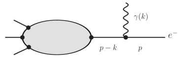
Figure 1: Photon-emission from an external electron in a generic process.

Disregarding ultraviolet (UV) divergences the only type of divergences that can arise in Feynman diagrams are due to propagators going on-shell which are of the IR-type. At LO this is particularly simple as we may just consider real emission of a photon from a charged particle, e.g. a lepton such as the electron $e^{-}$, as depicted in Fig. 2. The propagator $\frac{1}{(p+k)^{2}-m_{e}^{2}}$ denominator, for on-shell $p$, behaves like

$$(p+k)^{2}-m_{e}^{2}=2p\cdot k=2E_{\gamma}E_{e}(1-\beta\cos\theta)\;,$$ (1)

where $k=E_{\gamma}(1,0,0,1)$, $p=(E_{e},\kappa\hat{n})$, $E_{e}=\sqrt{m_{e}^{2}+\kappa^{2}}$, $\beta=\kappa/E_{e}$ and $\theta$ the angle between the unit vector $\hat{n}$ and the $z$-axis. The propagator is singular if either the photon energy $E_{\gamma}$ or the angle $\theta$ approach zero (and $m_{e}\to 0$). These divergences are known as soft and collinear respectively. In $d=4$ they lead to logarithmic singularities $\ln m_{\gamma}$ and $\ln m_{e}$. In certain regions of phase space these divergences combine and lead to soft-collinear divergences $\ln m_{\gamma}\,\ln m_{e}$. Generally, at $n$-loops there are terms of the order $\ln^{k}m_{\gamma}\,\ln^{l}m_{e}$ with $l\leq n$ and $k+l\leq 2n$.

It seems worthwhile to briefly digress on the collinear term $\ln m_{e}$. For finite lepton mass this is a physical effect, see for example the previously mentioned sizeable $\alpha\ln m_{e}/m_{b}$-terms in $B\to\pi e^{+}\bar{\nu}$. The question for what observables QED is well-defined for zero lepton masses, gave rise to the KLN-theorem (cf. App. A.2 for further comments). We shall assume leptons masses to be non-zero and special emphasis will be given to $\ln m_{\ell}$-terms to which we refer to as hard-collinear logs (cf. also App. B.3) and are a physical effect. This contrasts the terms caused by zero energy photons to which refer to as IR-divergences (and interchangeably as soft-divergences) following the main literature.

2.1 Observables are infrared finite

Of course physical observables have to be free of divergences and this is where one expects deep physical principles to dictate cancellations. Cancellations segregate observable from non-observable quantities. First, IR-divergences are interlinked with the very definition of what a particle is and the measurement process itself. How can one distinguish a single electron from an electron with an ultrasoft photon (or a highly relativistic electron with a photon emitted at an infinitesimally small angle)? That is also indeed where the resolution lies, what is measurable needs to be assessed carefully. One needs to come back to the idealisation mentioned in the introduction: infinite space and infinite detector resolution. The true IR-divergences (i.e. excluding collinear ones) are effectively regulated by the introduction of an energy scale, say $\delta$ (which has to be larger than the actual detector resolution scale). There are two main approaches to it:

1. The fixed particle Fock-space is abandoned in favour of so-called coherent states which take into account that charged particles are surrounded by a soft photon-cloud [29, 30, 31, 32, 33]. In 1970 Kulish and Faddeev [33] showed that the coherent state approach leads to a finite $S$-matrix in QED, which is gauge invariant with a separable Hilbert space.

2. Second, one defines observables which are inclusive enough such that these divergences cancel. This approach was pioneered by Bloch and Nordsieck 1937 [9], extended in the sixties by the KLN-theorem [10, 11] (cf. App. A.2) to additionally include collinear singularities and applied to correlation functions in form of the Kinoshita-Poggio-Quinn-theorem [10, 37, 38] (cf. Sec. 3.1). As a rule of thumb, the more inclusive a quantity is, the fewer divergences or IR-sensitive terms there are.

The second approach can, reassuringly, be seen as a limit of the latter. In view of it being more general we consider it worthwhile to first discuss the coherent state approach. Our brief summary is largely based on the excellent presentation in Duncan’s book [36] and some more context can be found in App. A.3. Let us concretely assume that the detector can only capture photons with an energy above $\delta$ and reject photons with energies above that threshold. Thus it is advisable to replace the electron state, to which we adhere for illustration, by a state with any number of photons with energies smaller than the detector cut-off

$$|e^{-}(\vec{q})\rangle\to|e^{-}(\vec{q})\rangle_{n}\equiv|e^{-}(q),\gamma(k_{1})\dots\gamma(k_{n})\rangle_{(E_{\gamma})_{i}<\delta}\;,$$ (2)

and (formally)

$$|e^{-}(\vec{q})\rangle=\sum_{n\geq 0,\vec{q}}c_{n}(\vec{q})|e^{-}(\vec{q})\rangle_{n}\;,$$ (3)

is the coherent state, with appropriate $c_{n}(\vec{q})$, which can be written as an exponential of an integral over the creation operators cf. App. A.3. Denoting by $P_{n}$ the probability of $n$-soft photon emission, the total probability is a sum of all possibilities $P_{\textrm{tot}}=\sum_{n\geq 0}P_{n}$. When the total transition probability $P_{\textrm{tot}}$ of all $n$-states (2) is considered, the momentum space integrals are cut-off below at $\delta$ and are thus manifestly IR-finite (no soft-divergences). The $S$-matrix is well-defined, as mentioned above, and the IR-divergences are absorbed into the definition of the states. It seems worthwhile to point out that this bears some resemblance with the absorption of the UV divergences into the parameters of the theory which in turn also originates from an idealisation, namely that space-time is a continuum.

How does this connect to the Bloch-Nordsieck mechanism? Reassuringly, upon expanding to finite order in $\alpha$ one recovers the Bloch-Nordsieck solution. More concretely, in order to compute the ${\cal O}(\alpha)$ corrections to a decay process $i\to f$ one has to consider its radiative counterpart $i\to f(\gamma_{E_{\gamma}<\delta})$. In the total transition probability one can show that the IR-divergences cancel diagram by diagram; as beautifully illustrated in many textbooks e.g. $e^{+}e^{-}\to\bar{q}q$ in [20]. These cancellations have been shown to hold to all orders in QED by exponentiation [39, 27].

No fixed particle-number $S$-matrix:

Let us briefly digress and motivate why the $S$-matrix of the fixed particle-number Fock space does not exist, as it turns out to be zero. We provide three different viewpoints:

1. The IR-divergences, caused by the absence of a mass gap, can be seen as an indication for the ill-defined fixed particle number Fock space $S$-matrix. It is instructive to give mass to the particle causing the trouble, the photon. The IR-divergences $\ln m_{\gamma}$ exponentiate such that the $S$-matrix, $S\propto\exp(|a|\ln m_{\gamma}+\dots)\to 0$, assumes zero value in the limit of zero photon mass. Hence, the $S$-matrix is infinite at fixed order and zero at all orders! Thus the asymptotic completeness of the in and out Hilbert space ceases to make sense as there is no $S$-matrix connecting the two.

2. Another way to look at it is to realise that due to the massless photons the single particle pole, assumed by the LSZ-formalism, is softened by the presence of radiative corrections $(p^{2}-m^{2})^{-1}\to(p^{2}-m^{2})^{-1+\alpha|A|}$ into a branch cut as first shown by Schroer in 2D model [40] (he came up with the term “infraparticle”). This makes the particle of mass $m$ disappear from the $S$-matrix when multiplied by the LSZ-factor $p^{2}-m^{2}$ upon taking the on-shell limit $p^{2}\to m^{2}$. Moreover, Buchholz [41] has shown, using very general arguments, that a charged particle obeying Gauss’ law cannot be a discrete eigenstate of the momentum squared operator, which goes hand in hand with the branch cut. A notable aspect is that the coefficient $|A|$ is gauge dependent, e.g. [42], and another sign that there is a problem.

3. Whereas the $S$-matrix is gauge invariant in perturbation theory this is not the entire story as has recently been shown using asymptotic symmetries [43]. The common lore is that local gauge symmetries give rise to global charge conservation only and that local gauge symmetries are not really symmetries in the observable sense. However, asymptotically (that is at spatial infinity) there are infinitely many symmetries, so-called asymptotic symmetries [44], known as large (i.e. non-local) gauge symmetries. In a very interesting paper [43] it has been shown that the vanishing of the fixed particle number $S$-matrix can be understood as due to non-invariance under these asymptotic symmetries. Closing the circle, it is found that once gauge invariance is enforced, the coherent states emerge!

Now, is it considered a problem that the fixed particle number $S$-matrix is not defined? For mathematical physics, yes. The fact that electron does not correspond to an isolated particle in the spectrum is known as the IR-problem of QED (e.g. [45] also for historic references and discussion of this notorious problem). The pragmatic particle physicist, or advocate of the Bloch-Nordsieck- and KLN-approach, would simply point to the fact that the fixed particle number $S$-matrix is not an observable but rather an intermediate auxiliary quantity.

Concluding, in practice the infrared problem of QED is bypassed in the pragmatic approach by IR-regularisation (e.g. $m_{\gamma}\neq 0$) and removing the regulator ($m_{\gamma}\to 0$) in observables such as decay rates. Let us add that in practice, for a number of reasons (e.g. no additional scale), dimensional regularisation is the choice by most practitioners.

3 Decay Rates and their Infrared-effects

Following the discussion on the origin of IR-divergences and why they disappear from observables we discuss these mechanisms in three practical examples with decreasing level of inclusiveness and increasing level of IR-effects. Namely, the (inclusive) $e^{+}e^{-}\to hadrons$ cross section, the leptonic decay $\pi^{+}\to\ell^{+}\bar{\nu}$ and the semileptonic case $B\to\pi\ell^{+}\bar{\nu}$. In the latter two cases, the hadrons will be treated in the point-like approximation with comments beyond this treatment deferred to Sec. 4.

For most practical applications first order ${\cal O}(\alpha)$ is sufficient. At the amplitude level we therefore need ${\cal O}(e^{0,1,2,})$, denoted by ${\cal A}^{(0,1,2)}$, corresponding to tree, real and virtual. We refer to ${\cal A}^{(0)}$ and ${\cal A}^{(2)}$ as the non-radiative and to ${\cal A}^{(1)}$ as the radiative amplitude. The cancellation of IR-divergences is then a result of $\textrm{Re}[{\cal A}^{(0)}({\cal A}^{(2)})^{*}]$ versus $|{\cal A}^{(1)}|^{2}$ when properly integrated over phase space. Let us rephrase this in terms of a generic decay $i\to f$ at the level of the rates

$$d\Gamma(i\to f) \;\propto\; 1+ \frac{\alpha}{\pi}(A_{V}\ln m_{\gamma}+B_{V}\ln m_{\gamma,f}\ln m_{f}+C_{V}\ln m_{f}+{\cal O}(1))d\Phi_{f}\;,$$

$$d\Gamma(i\to f\gamma) \;\propto\; \frac{\alpha}{\pi}(A_{R}\ln m_{\gamma}+B_{R}\ln m_{\gamma,f}\ln m_{f}+C_{R}\ln m_{f}+{\cal O}(1))d\Phi_{f}d\Phi_{\gamma}\;,$$ (4)

where $d\Phi$ is the phase space measure, $m_{f}$ is a small mass of a final state particle (e.g. an electron mass) and $m_{\gamma,f}$ stands for either $m_{f}$ or $m_{\gamma}$. The subscripts $V$ and $R$ denote virtual and real and $A$, $B$ and $C$ stand for soft, soft-collinear and hard-collinear divergences. Integrating over the entire photon phase space

$$d\Gamma(i\to f)+\int d\Phi_{\gamma}\,d\Gamma(i\to f\gamma)\propto(1+\frac{\alpha}{\pi}C\ln m_{f}+{\cal O}(1))\,d\Phi_{f}\;,$$ (5)

with all the soft-divergences canceling and the collinear logs cancel,

$$C=(C_{V}+\int d\Phi_{\gamma}C_{R})=\left\{\begin{array}[]{ll}\textrm{zero}&\textrm{collinear-safe differential variables}\\[2.84544pt] \textrm{non-zero}&\textrm{non collinear -safe differential variables}\end{array}\right.\;,$$ (6)

depending on the differential variables (cf. Sec. 3.3 for a concrete example). The further statement of the cancellation-theorems (Bloch-Nordsieck and KLN) is that that if one integrates over the remaining phase space $d\Phi_{f}$, then (in the total rate)

$$\Gamma(i\to f)+\Gamma(i\to f\gamma)\propto 1+\frac{\alpha}{\pi}{\cal O}(1)\;,$$ (7)

all IR-divergences are absent, schematically: $([A,B,C]_{V}+[A,B,C]_{R})^{\textrm{inc}}=0$. This picture is broken in practice by the following two sources:

• The experiment is not fully photon-inclusive and rejects hard photons with $E_{\gamma}>\delta$ where $\delta$ is the previously discussed threshold which is (slightly) larger than the actual detector resolution. This leads to the replacements

  $$(A_{V}+A_{R})\ln m_{\gamma} \;\to\; (A_{V}(\delta)+A_{R}(\delta))\ln\delta\;,$$

  $$(B_{V}+B_{R})\ln m_{\gamma}\ln m_{f} \;\to\; (B_{V}(\delta)+B_{R}(\delta))\ln\delta\ln m_{f}\;,$$

  $$C\ln m_{f} \;\to\; C(\delta)\ln m_{f}\;,$$ (8)

  where $C(\delta)\neq 0$ irrespective of whether the differential variables are collinear-safe or not. The functions $A,B,C(\delta)$ are polynomial in $\delta$.

• The rate can be differential in some final state kinematics and therefore not a total rate as in (5). In this case the unitarity argument, on which the cancellation is based, does not necessarily hold since the kinematics make the sum too restrictive. The (non)-cancellation needs to be reassessed, depending on the kinematic variables hard-collinear effects $\ln m_{f}$ do or do not cancel.

type	i) diff. in $\gamma$	ii) diff. in $f$	IR-terms	Sec.
$e^{+}e^{-}\to hadrons$	no	no	none	3.1
$\pi^{+}\to\ell^{+}\bar{\nu}$	yes	no	$A,B,(C)$ Eqs.(3,i))	3.2
$B\to\pi\ell^{+}\bar{\nu}$	yes	yes	$A,B,C$ Eqs.(3,i))	3.3

Table 1: Types of observables considered where diff. is short for differential in $\gamma$ or $f$ (final states) and i) and ii) refer to the itemised conditions above. The bracket around (C) in row 2 will, hopefully, become clear upon reading Sec. 3.2.

3.1 A classic example of infrared finiteness: $e^{+}e^{-}\to hadrons$

Here we briefly deviate from the QED-course as we consider finiteness under correction in the strong coupling constant to $e^{+}e^{-}\to hadrons$. An analogue in QED would be the somewhat exotic $\nu\bar{\nu}\to Z\to\ell^{+}\ell^{-}$. Now, by the optical theorem the total cross-section

$$\sigma_{\textrm{tot}}(e^{+}e^{-}\to hadrons)(q^{2})\propto\textrm{Im}[\Pi(q^{2})]\;,$$ (9)

is related to the imaginary part of the vacuum polarisation $\Pi(q^{2})$

$$\left(q_{\mu}q_{\nu}-q^{2}g_{\mu\nu}\right){\Pi}(q^{2})=i\int d^{4}xe^{ix\cdot q}\langle 0|Tj_{\mu}(x)j_{\nu}(0)|0\rangle\;,$$ (10)

where $j_{\mu}=\sum_{f}eQ_{f}\bar{f}\gamma_{\mu}f$ is the electromagnetic current and $Q_{f}$ the electromagnetic charge. On the non-perturabative level there is no question as to whether this quantity is well-defined because of the mass gap. In particular, in the large-$N_{c}$ limit

$$\textrm{Im}[\Pi(s)]=\pi\sum_{V=\rho^{0},\omega..}\delta(s-m_{V}^{2})f_{V}^{2}\;,$$ (11)

with $f_{V}$ the vector meson decay constants and most importantly $m_{\rho^{0}}\approx 770\,\mbox{MeV}$ is the lowest mass exhibiting the mass gap. The question we would like to address is whether it is finite to all orders in perturbation theory using quarks and gluons as degrees of freedom.

According to the cancellation-theorems and the discussion outlined in the beginning of this section this must be the case since this is a fully inclusive observable (and conditions i) & ii) are not met). Alternatively, this can be established on grounds of the Kinoshita-Poggio-Quinn-theorem [10, 37, 38] which states: In massless renormalisable theories the one-particle irreducible correlation functions are IR-finite for non-exceptional (external) Euclidean momenta. Renormalisability is important as it settles power counting for the proof and the Euclidean momenta condition avoids particles going on-shell. This applies to the case at hand since $\textrm{Im}[\Pi(q^{2})]=\frac{1}{2i}(\Pi(q^{2}+i0)-\Pi(q^{2}-i0))$ with $q^{2}\pm i0$ effectively counts as off-shell (or Euclidean in practice). Hence $\sigma_{\textrm{tot}}(q^{2})$ must be IR-finite (in perturbation theory) as found in many explicit computations for any $q^{2}>0$ in particular.

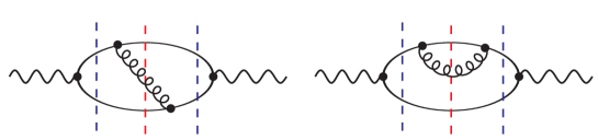
Figure 2: Strong coupling corrections to the vacuum polarisation $\Pi(q^{2})$ (10), at $O(\alpha_{s})$, which necessarily involves quarks and gluons (partons). As its imaginary part corresponds to the total cross section (9) the cuts give rise to various subprocesses which include the virtual and real parts. The dashed or blue cuts correspond to the virtual and the real parts respectively.

One can learn a fair amount by considering the one-loop corrections (depicted in Fig. 2) since the imaginary part is proportional to the discontinuity and the latter is proportional to the sum of all cuts by the Cutkosky rules (e.g. [18]) The different types of cuts include the radiative and non-radiative parts cf. figure caption. Each one of these cuts is IR-divergent but they cancel in the sum as dictated by the arguments given above. That individual contributions behave very different from the total contribution is not restricted to IR-effects but can also appear in the power-behaviour of a heavy quark mass or an external momentum in case they are assumed to be large.

3.2 Leptonic decay of the type $\pi^{+}\to\ell^{+}\bar{\nu}$

We now turn to the simple example of an exclusive decay, the pion decay $\pi^{+}\to\ell^{+}\bar{\nu}$. The photon energy cut-off $E_{\gamma}<\delta$ (in say the pion restframe) will introduce the $\ln\delta$-terms as in (i)). This will lead to soft- and soft-collinear terms as indicated in Tab. 1. The hard-collinear logs ($C$-type in (3)) are a bit peculiar in this decay in the SM since the amplitude is ${\cal O}(m_{\ell})$ (and therefore automatically finite in the limit $m_{\ell}\to 0$). This helicity suppression is relieved for $S\!-\!P$ interactions and we thus include them along the $V\!-\!A$ structure in order to illustrate the straightforward nature of the hard-collinear logs in this example. In turn these logs have to disappear in the photon-inclusive limit $2m_{\pi}\delta\to m_{\pi}^{2}-m_{\ell}^{2}$. All of which will be made explicit.

The four-Fermi effective Lagrangian, including $S\!-\!P$- and $V\!-\!A$-interactions, reads

$${\cal L}^{\textrm{eff}}=4\sqrt{2}G_{F}\left(C_{V\!-\!A}\bar{u}\gamma_{\mu}d_{L}\bar{\ell}\gamma^{\mu}\nu_{L}+C_{S\!-\!P}\bar{u}d_{L}\bar{\ell}\nu_{L}\right)\;,$$ (12)

where $2f_{L}\equiv(1-\gamma_{5})f$ and in the SM $(C_{V\!-\!A},C_{S\!-\!P})=(V_{\textrm{ud}},0)$. The LO amplitude is given by

$${\cal A}^{(0)}(\pi^{+}\to\ell^{+}\bar{\nu}) \;\propto\; C_{V\!-\!A}(L_{0})_{\mu}H^{\mu}_{0}+C_{S\!-\!P}L_{0}H_{0}$$

$$\;=\; i(C_{V\!-\!A}m_{\ell}F_{\pi}-C_{S\!-\!P}G_{\pi})L_{0}\;,$$ (13)

where the leptonic matrix element reads

$$L_{0}^{(\mu)}\equiv\langle\bar{\nu}\ell^{+}|\bar{\ell}\Gamma^{(\mu)}\nu|0\rangle=\bar{u}(p_{\nu})\Gamma^{(\mu)}\nu(p_{\ell})\;,$$ (14)

with $\Gamma=(1-\gamma_{5})$, $\Gamma_{\mu}=\gamma_{\mu}\Gamma$ and the hadronic matrix elements are

$$\langle 0|A^{a}_{5\,\mu}|\pi^{b}(p)\rangle \;=\; \delta^{ab}(H_{0})_{\mu} \;=\; \phantom{-}i\delta^{ab}F_{\pi}p_{\mu}\;,$$

$$\langle 0|P^{a}|\pi^{b}(p)\rangle \;=\; \delta^{ab}H_{0} \;=\; -i\delta^{ab}G_{\pi}\;,\quad G_{\pi}=\frac{F_{\pi}m_{\pi}^{2}}{2m_{q}}=\frac{-\langle\bar{q}q\rangle}{2F_{\pi}}\;,$$ (15)

with $A^{a}_{5\,\mu}=\bar{q}T^{a}\gamma_{\mu}\gamma_{5}\,q$, $P^{a}=\bar{q}T^{a}\gamma_{5}\,q$ and $T^{a}$ the adjoint $SU(2)$-representation matrix corresponding to $q=(u,d)$ (with (u)p and (d)own quarks). Note that use of the equation of motion was made for the $V\!-\!A$-part in (3.2) which makes the $m_{\ell}$-suppression factor explicit. The LO decay rate is given by

$$\Gamma(\pi^{+}\to\ell^{+}\bar{\nu})^{(0)}=\frac{G_{F}^{2}}{\pi m_{\pi}^{3}}|C_{V\!-\!A}m_{\ell}F_{\pi}-C_{S\!-\!P}G_{\pi}|^{2}|\vec{p}_{\ell}|^{2}\;,$$ (16)

where the lepton velocity, in the pion’s restframe, is

$$\quad|\vec{p}_{\ell}|=\frac{\lambda^{1/2}(m_{\pi}^{2},m_{\ell}^{2},0)}{2m_{\pi}}=\frac{m_{\pi}}{2}\left(1-\frac{m^{2}_{\ell}}{m_{\pi}^{2}}\right)\;,$$ (17)

and $\lambda(x,y,z)\equiv x^{2}+y^{2}+z^{2}-2xy-2xz-2yz$ denotes the Källèn function. Notably $F_{\pi}\approx 92\,\mbox{MeV}$, a non-perturbative parameter of QCD known as the pion decay constant, is the order parameter of the spontaneous breaking of chiral symmetry $SU(2)_{L}\times SU(2)_{R}\to SU(2)_{V}$ (in the $m_{q}\to 0$ limit). When QED corrections are considered it ceases to be an observable and it is essentially degraded to the status of a wave function renormalisation constant. This can be seen from the explicit results in the nice review [46] where $F_{\pi}$ is found to be gauge dependent and divergent in the $m_{\pi}\to 0$ limit. Unlike in QCD, in QED the chiral logs $\ln m_{\pi}$ are not protected by powers in the pion mass since $F_{\pi}$ is not an observable. This is a point we will come back to at the end of the section.

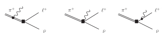
Figure 3: Real emission diagram of the pion decay. The diagram in the centre is the so-called contact term and does appear for the $V\!-\!A$- but not the $S\!-\!P$-interaction. The real amplitude is given in (3.2).

Next we discuss how to incorporate radiative corrections in the point-like approximation. This is a straightforward exercise in effective field theory. The hadronic operator are matched to pions ($\langle 0|\pi^{a}|\pi^{b}\rangle=\delta^{ab}$)

$$A^{a}_{5\,\mu}\to-F_{\pi}D_{\mu}\pi^{a}\;,\quad P^{a}\to-iG_{\pi}\pi^{a}\;,$$ (18)

such that the LO matrix element (3.2) is reproduced. The momentum dependence in the axial current (3.2) enforces a covariant derivate, $D_{\mu}\pi^{a}=(\partial_{\mu}+ieQ_{\pi^{a}}A_{\mu})\pi^{a}$, which gives raise to a so-called contact term. The leading radiative amplitude is given by

$${\cal A}^{(1)}(\pi^{+}\to\ell^{+}\bar{\nu}\gamma)\propto\sum_{i}C_{i} \left(\hat{Q}_{\ell_{1}}\bar{u}\frac{2\epsilon^{*}\cdot\hat{\ell}_{1}+\not{\epsilon}^{*}\not{k}}{2k\cdot\hat{\ell}_{1}}(\Gamma\cdot H_{0})_{i}v+\hat{Q}_{\bar{\ell}_{2}}\bar{u}(\Gamma\cdot H_{0})_{i}\frac{2\epsilon^{*}\cdot\hat{\ell}_{2}+\not{k}\not{\epsilon}^{*}}{2k\cdot\hat{\ell}_{2}}v\;+\right.$$

$$\left.\hat{Q}_{\pi}(L_{0}\cdot H_{0})_{i}|_{p\to\bar{p}}\frac{\epsilon\cdot(\hat{p}+\hat{\bar{p}})}{2k\cdot\hat{p}}+\hat{Q}_{\pi}(L_{0}\cdot H_{0})_{i}|_{p\to\epsilon^{*}}\right)\;,$$ (19)

where $\bar{p}=p-k$, $\ell,\nu\to\ell_{1},\ell_{2}$ in order to be more general, $i=S\!-\!P,V\!-\!A$ and the conventions are the same as in [47]: $\hat{Q}_{j}=\pm Q_{j}$ and $\hat{p}_{j}=\pm p_{j}$ for out(in)-going states. Some more detail on the notation. The last term in (3.2), and centre of Fig. 3, is the so-called contact term, only present for $V\!-\!A$ as mentioned above. In addition, the following compact notation has been introduced

$$(L_{0}\cdot H_{0})_{i}=\left\{\begin{array}[]{ll}(L_{0})_{\mu}H^{\mu}_{0}&i=V\!-\!A\\[2.84544pt] L_{0}H_{0}&i=S\!-\!P\end{array}\right.\;,$$ (20)

likewise for $L_{0}\to\Gamma$. The terms of the Low-theorem (cf. App. A.1) are explicit which include the ${\cal O}(E_{\gamma}^{-1})$ eikonal terms

$${\cal A}^{(1)}={\cal A}^{(0)}\sum_{i}\hat{Q}_{i}\frac{\epsilon^{*}\cdot\hat{p}_{i}}{k\cdot\hat{p}_{i}}+{\cal O}(E_{\gamma}^{0})\;,$$ (21)

and the ${\cal O}(E_{\gamma}^{0})$-term related to the angular momentum can be seen in the leptonic parts. Gauge invariance amounts to ${\cal A}^{(1)}|_{\epsilon\to k}=0$ and does hold provided $\sum_{i}\hat{Q}_{i}=\hat{Q}_{\ell_{1}}+\hat{Q}_{\bar{\ell}_{2}}+\hat{Q}_{\pi}=0$ (which is nothing but charge conservation). The latter has to be imposed in gauge-fixed perturbation theory but would be automatic in a manifestly gauge invariant formalism such as the path-integral used in lattice simulations. Hence the radiative amplitude is gauge invariant and thus the virtual (or non-radiative) amplitude must be as well. In particular in the virtual amplitude the gauge dependence of the ${\cal O}(\alpha)$ pion decay constant cancels against the lepton-pion and lepton radiative corrections. As previously said, we present the $S\!-\!P$- and $V\!-\!A$-interaction separately as they both have different features.

3.2.1 Leading logs with $S\!-\!P$-interaction

For the $S\!-\!P$-interaction ($C_{S\!-\!P}\neq 0,\,C_{V\!-\!A}=0$) we may parameterise the ${\cal O}(\alpha)$ rate as follows

$$\Gamma(\pi^{+}\to\ell^{+}\bar{\nu})=\Gamma(\pi^{+}\to\ell^{+}\bar{\nu})^{(0)}(1+\frac{\alpha}{4\pi}\left(F_{\textrm{soft}}(\hat{m}^{2}_{\ell},2\hat{\delta})+F_{\textrm{coll}}(\hat{\delta})\ln\hat{m}_{\ell}+\textrm{non-log}\right))\;,$$ (22)

where “non-log” stands for anything that is neither a soft, soft-collinear or hard-collinear log. Hatted quantities, except charges, are understood to be divided by the pion mass in this section. The quantity $\delta$ is the previously introduced photon energy cut-off and its photon-inclusive limit is $2\hat{\delta}\to 1-\hat{m}_{\ell}^{2}$. Below we discuss both $F_{\textrm{soft}}$ and $F_{\textrm{coll}}$ without resorting to the full computation.

• The soft and soft-collinear terms are universal and given by

  $$F_{\textrm{soft}}(x,y)=-(4\frac{1+x^{2}}{1-x^{2}}\ln x^{2}+8)\ln y\;,$$ (23)

  and its exponentiation is a well established [39, 27]

  $$\Gamma(\alpha\to\beta)=\Gamma(\alpha\to\beta)^{\textrm{LO}}\exp(-A\ln\frac{\lambda}{\Lambda})\;,\quad$$ (24)

  where $\lambda$ and $\Lambda$ are IR and UV cut-offs. These are to be replaced in practice with $\delta$ and the largest scale in the problem; beyond that they are equivalent to so-called finite terms and undetermined in the leading log approximation. Now, the factor $A$ has a pleasing form

  $$A=\frac{e^{2}}{8\pi^{2}}\sum_{i,j}\hat{Q}_{i}\hat{Q}_{j}\frac{1}{2\beta_{ij}}\ln\frac{1+\beta_{ij}}{1-\beta_{ij}}\;,$$ (25)

  where the sum is over the charged particles in the decay and

  $$\beta_{ij}=\frac{\beta_{i}+\beta_{j}}{1+\beta_{i}\beta_{j}}\;,$$ (26)

  is the relativistic addition of the velocities of the $i,j$-particles in the $ij$-restframe. With $\beta_{ii}=1$ for $i=\pi^{+},\ell^{+}$ (since the relative velocities are zero ) and with $\beta_{\ell\pi}=(1-\hat{m}_{\ell}^{2})/(1+\hat{m}_{\ell}^{2})$ one recovers $\eqref{eq:soft}$.

  It is instructive to reproduce the leading term from the eikonal part (21) which is of course what the original papers did. Following [47] we denote the decay rate as

  $$d\Gamma \;=\; d\Gamma^{\textrm{LO}}+\frac{\alpha}{\pi}\sum_{i,j}\hat{Q}_{i}\hat{Q}_{j}({\cal H}_{ij}+{\cal F}_{ij}(\delta))d\phi_{f}=d\Gamma^{\textrm{LO}}(1+\Delta_{\text{rel}}\,d\phi_{f})\;,$$ (27)

  where ${\cal H}$ and ${\cal F}$ stand for the non-radiative and the radiative part respectively and $\Delta_{\text{rel}}$ is the relative correction, not to be confused with the photon energy cut-off, which is a function of the non-trivial differential variables $d\phi_{f}=\prod_{i=1}^{n_{f}}d\vartheta_{i}$ (with $n_{f}=0$ and $n_{f}=2$ in the leptonic and semileptonic case respectively). After making use of gauge invariance, by choosing the Feynman gauge $\xi=1$, performing the polarisation sum $\sum_{\lambda}\epsilon^{*}_{\mu}(\lambda)\epsilon_{\nu}(\lambda)=-g_{\mu\nu}+(1-\xi)k_{\mu}k_{\nu}/k^{2}\to-g_{\mu\nu}$ over the eikonal part one gets

  $${\cal F}_{ij}(\delta)=(2\pi)^{2}\int_{\delta}\frac{-{p}_{i}\cdot{p}_{j}}{(k\cdot{p}_{i})(k\cdot{p}_{j})}d\Phi_{\gamma}=-K_{R}(\delta)I_{ij}^{(0)}+\textrm{non-soft}\;,$$ (28)

  where “non-soft” stands for finite non-logarithmic regularisation dependent terms. The $K_{R}(\delta)$-term is the regularisation dependent energy integral and $I_{ij}^{(0)}$ an angular integral. In the leading log approximation $K_{R}(\delta)$ and $I_{ij}^{(0)}$ are separately Lorentz invariant [47]. This is non-trivial since the introduction of the photon energy cut-off introduces a preferred frame and complicates the analytic evaluation of the non-approximated integrals. More concretely,

  $$K_{R}(\delta)=\int_{0}^{\delta}\frac{dE_{\gamma}}{E_{\gamma}}=\left\{\begin{array}[]{ll}-\frac{1}{2}\ln\frac{m_{\gamma}}{\mu}+\ln\left(\frac{\delta}{\mu}\right)+{\cal O}(m_{\gamma})&m_{\gamma}\textrm{-reg}\\ -\frac{1}{2\epsilon}+\ln\left(\frac{2\delta}{\mu}\right)+{\cal O}(\epsilon)&\text{dim-reg}\end{array}\right.\;,$$ (29)

  given in dimensional regularisation $d=4-2\epsilon$ and photon mass regularisation (cf. App. D [47] for some more detail). The angular integral produces a term

  $$I_{ij}=\int d\Omega\frac{E_{\gamma}^{2}p_{i}\cdot p_{j}}{(k\cdot p_{i})(k\cdot p_{j})}=\frac{1}{2\beta_{ij}}\ln\frac{1+\beta_{ij}}{1-\beta_{ij}}=1+{\cal O}(\beta_{ij})\;,$$ (30)

  which matches the expression in (25) and thus reproduces (23) as outlined earlier.

• The hard-collinear logs can be obtained from the splitting function which has been verified in [47] for the more advanced semileptonic case. The formula for the collinear logs reads

  $$\Delta_{\text{rel}}|_{\ln m_{\ell}} \;=\; -\frac{\alpha}{\pi}\hat{Q}^{2}_{\ell^{+}}\ln\hat{m}_{\ell}\left(\frac{d\Gamma^{\textrm{LO}}}{d\phi_{f}}\right)^{-1}\int^{1}_{z(\hat{\delta})}dzP_{f\to f\gamma}(z)\frac{d\Gamma^{\textrm{LO}}}{d\phi_{f}}(f_{i}(z)\vartheta_{i})$$

  $$\;\to\; -\frac{\alpha}{\pi}\hat{Q}^{2}_{\ell^{+}}\ln\hat{m}_{\ell}\int^{1}_{1-2\hat{\delta}}{dz}P_{f\to f\gamma}(z)$$

  $$\;=\; -\frac{\alpha}{\pi}\hat{Q}^{2}_{\ell^{+}}\ln\hat{m}_{\ell}\left(\frac{3}{2}-2\hat{\delta}(2-\hat{\delta})\right)\;,$$ (31)

  (and thus $F_{\textrm{coll}}(\hat{\delta})=-4\hat{Q}^{2}_{\ell^{+}}(\frac{3}{2}-2\hat{\delta}(2-\hat{\delta})$) with fermion splitting function

  $$P_{f\to f\gamma}(z)=\frac{1+z^{2}}{(1-z)_{+}}+\frac{3}{2}\delta(1-z)\;,$$ (32)

  where $\delta(1-z)$ is a Dirac delta function and $\frac{1}{(1-z)_{+}}$ is the plus distribution $\int_{0}^{1}dz\frac{f(z)}{(1-z)_{+}}=\int_{0}^{1}dz\frac{f(z)-f(1))}{1-z}$. For the leptonic case the formula is trivial since there are no phase space variables. Crucially, in the photon-inclusive limit $2\hat{\delta}\to 1$ the hard-collinear logs cancel $F_{\textrm{coll}}(\frac{1}{2})=0$ in accordance with the KLN-theorem. This has to hold since $\int_{0}^{1}dzP_{f\to f\gamma}(z)=0$ which in turn follows from the conservation of the electromagnetic current (as it is related to the current’s anomalous dimension which vanishes).

3.2.2 Leading order result with $V\!-\!A$-interaction as in the Standard Model

The Standard Model computation ($C_{S\!-\!P}=0,\,C_{V\!-\!A}\neq 0$) has of course been obtained a long time ago [48, 49], we quote

$$\Gamma(\pi^{+}\to\ell^{+}\bar{\nu})=\Gamma(\pi^{+}\to\ell^{+}\bar{\nu})^{(0)}(1+\frac{\alpha}{4\pi}\left(-3\ln\hat{m}_{W}^{2}+F(\hat{m}^{2}_{\ell},2\hat{\delta})\right))\;,$$ (33)

and comment on the various terms further below. In (33) $-3\ln{\hat{m}_{W}^{2}}$ incorporates the matching to the $M_{W}$-scale [49]. The explicit radiative function $F(x,y)$ is given by [50]

$$F(x,y) \;=\; 4\frac{1+x^{2}}{1-x^{2}}Li_{2}(y)+\ln x^{2}+\frac{2-10x^{2}}{1-x^{2}}\ln x^{2}-4\frac{1+x^{2}}{1-x^{2}}Li_{2}(1-x^{2})-3$$

$$\;+\; \frac{3+y^{2}+4y(x^{2}-1)}{2(1-x^{2})^{2}}\ln(1\!-\!y)+\frac{y(4\!-\!y\!-\!x^{2})}{(1-x^{2})^{2}}\ln x^{2}+\frac{y(22-3y-28x^{2})}{2(1-x^{2})^{2}}$$

$$\;+\; F_{\textrm{soft}}(x,y)\;.$$ (34)

In the photon-inclusive case, $F_{\textrm{inc}}(x)\equiv F(x,1-x^{2})$, the radiative function assumes the form

$$F_{\textrm{inc}}(x) \;=\; -8\ln(1-x^{2})-\frac{3x^{2}}{(1-x^{2})^{2}}\ln x^{2}-8\frac{1+x^{2}}{1-x^{2}}Li_{2}(1-x^{2})$$

$$\;+\; \frac{13-19x^{2}}{2(1-x^{2})}+\frac{6-14x^{2}-4(1+x^{2})\ln(1\!-\!x^{2})}{1-x^{2}}\ln x^{2})\;.$$ (35)

Let us now turn our focus to the logs as in the previous section:

• The soft and soft-collinear terms are universal and $F_{\textrm{soft}}(x,y)$ is indeed the same function as in (23).

• Hard-collinear logs, of the type $\ln m_{\ell}$, are not present. The LO $V\!-\!A$-amplitude is ${\cal O}(m_{\ell})$-suppressed. and this is enough to guarantee the absence of the latter at ${\cal O}(\alpha)$ which can be seen as follows. In the real radiation rate the $\ln m_{\ell}$-terms arise from the eikonal part (21) which are proportional to the LO amplitude which is ${\cal O}(m_{\ell})$ and thus the logs can be at worst of the form $m^{2}_{\ell}\ln m_{\ell}^{2}$ in the rate. Since the $\ln m_{\ell}$-terms in the virtual and the real part of the ${\cal O}(\alpha)$ rate have to cancel the virtual rate cannot contain them either. We are to conclude that ${\cal O}(\alpha)m_{\ell}^{2}\ln m_{\ell}$ are the leading logs of this type. Since the limit $m_{\ell}\to 0$ is not divergent these logs do not have to cancel contrary to the $S\!-\!P$-case. Inspection of (3.2.2) shows that they do indeed not cancel since $F=-3\hat{m}_{\ell}^{2}\ln\hat{m}_{\ell}^{2}+\dots$. It seems worthwhile to briefly pause and reflect. If the “naive” equation of motion, linking $V\!-\!A$ to $S\!-\!P$, where to apply it would be possible to reuse $S\!-\!P$-computation from the one of $V\!-\!A$. This holds for the real part but not the virtual part as in this case the photon in the derivative interaction is not an external on-shell particle.

  The moral of the story is that collinear logs only cancel if they have to due to the principle of unitarity which underlies the KLN-theorem.

• A different type of collinear log: We may however turn the tables and consider the decay $\tau^{-}\to\pi^{-}\bar{\nu}$ and regard $\ln m_{\pi}$ as the collinear log. The amplitude which is identical to the one for the leptonic decay is not ${\cal O}(m_{\pi})$-suppressed, thus there will be $\ln m_{\pi}$ terms in the real and the virtual part of the rate and they have to cancel in the total rate. There are some differences in the integration over phase space for the radiative part but not for the relevant eikonal terms. Inspecting (3.2.2), taking the $1/x\to 0$ limit and adding the log in (33), one collects $\frac{\alpha}{4\pi}(6+16+6+0+0-28)\ln m_{\pi}=0$ and it is seen that the logs do cancel as they have to!

3.3 Semileptonic decay of the type $B\to\pi\ell^{+}\bar{\nu}$

The new element in the semileptonic decay $B\to\pi\ell^{+}\bar{\nu}$ is the extra meson in the final state leading to two non-trivial kinematic variables. They can be chosen to be the Dalitz-plot variables or the more commonly used lepton momentum squared $q^{2}=(\ell_{1}+\ell_{2})^{2}$ and the angle $\theta$ of a lepton to the decay axis in the $q$-restframe (as depicted in Fig. 4). Hence the LO decay is differential unlike in the leptonic case (cf. for instance App. B.1 in [47] for the explicit result). A noticeable aspect is that QED, unlike the weak interaction term (12), give rise to higher moments in the lepton angle [51].

In many ways the QED-treatment of the semileptonic decay $B\to\pi\ell^{+}\bar{\nu}$ in the point-like approximation is similar to the leptonic decay and we shall be brief on those matters. There are also new aspects which bring in a certain amount of complication which we identify and examine more closely:

1. The role of the pion decay constant $F_{\pi}$ is taken by two form factors $f^{B\to\pi}_{\pm}(q^{2})$,

   $$\langle 0|A^{a}_{5\,\mu}|\pi^{b}(p)\rangle \;=\; -i\delta^{ab}F_{\pi}p_{\mu}\to$$

   $$\langle\pi|V_{\mu}|B\rangle \;=\; f^{B\to\pi}_{+}(q^{2})(p_{B}\!+\!p_{\pi})_{\mu}+f^{B\to\pi}_{-}(q^{2})(p_{B}\!-\!p_{\pi})_{\mu}\;.$$ (36)

   Often in the literature the form factor is taken to be a constant, which is a good approximation in $K\to\pi\ell^{+}\bar{\nu}$ but less so for $B\to\pi\ell^{+}\bar{\nu}$. Expanding the form factor in $q^{2}$, as in [47], leads to a more involved effective theory which goes beyond the point-like approximation. The effect of the expansion is most prominent when the photon energy cut is large due to migration of radiation (for which we refer the reader to the plots in App. A in[47]).

2. For the radiative matrix element the $(q^{2},\theta)$-variables have to be adapted because of the additional photon. We follow the discussion in [47] (replacing the kaon by the pion) where the following kinematic variables

   $$\{q^{2}_{a},c_{a}\}=\left\{\begin{array}[]{ll}q_{\ell}^{2}=(\ell_{1}+\ell_{2})^{2}\;,{}&c_{\ell}=-\left(\frac{\vec{\ell_{1}}\cdot\vec{p}_{\pi}}{|\vec{\ell_{1}}||\vec{p}_{\pi}|}\right)_{q-\textrm{RF}}\\ q^{2}_{0}=(p_{B}-p_{\pi})^{2}~{},&c_{0}=-\left(\frac{\vec{\ell_{1}}\cdot\vec{p}_{\pi}}{|\vec{\ell_{1}}||\vec{p}_{\pi}|}\right)_{q_{0}-\textrm{RF}}\;,\end{array}\right.$$ (37)

   are defined with $q-\textrm{RF}$ and $q_{0}-\textrm{RF}$ denoting the $q$ and $q_{0}\equiv q+k$ restframes respectively. Note that, the $(q_{0}^{2},c_{0})$-variables, unlike at an $e^{+}e^{-}$-collider, are difficult to measure at a hadron collider where the components of the $B$-momentum are unknown.

3. The LO amplitude is not ${\cal O}(m_{\ell})$-suppressed and a priori it is only the total (photon-inclusive) rate which is well-defined in the $m_{\ell}\to 0$ limit. As previously state, for finite $m_{\ell}$, as in the real world, this leads to a sizeable and measurable effect. This raises the interesting question as to whether any of the differential variables in (37) are collinear-safe (i.e. $m_{\ell}\to 0$ can be taken).

4. The photon interacts with many particle-pairs and this complicates the analytic evaluation of the phase-space integrals as one can choose the restframe only once. As previously discussed, the energy- and soft-integrals (30) are separately Lorentz-invariant in the soft-limit and can therefore each be evaluated using a separate preferred frame [47].

Now, point 4 is partly covered in App. B.2 and all aspects of point 1 are covered in [47]. Let us just briefly mention that as long as a constant form factor is assumed or the mesons are neutral, the computation of the real and virtual amplitude is very similar to the leptonic case albeit technically more involved. Points 2 and 3 deserve a closer look and are the topic of the next section.

3.3.1 (Non)-collinear safe differential variables

The soft-divergences which have to cancel at the differential level, can of course be derived using the same techniques as for the lepton case (24) (with relevant practical remarks deferred to App. B.2). The hard-collinear divergences have been isolated using the phase space slicing technique. They cancel charge by charge in the photon-inclusive total rate in accordance with (7).

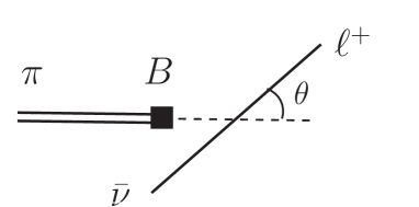
Figure 4: Sketch of semileptonic (non-radiative) decay $B\to\pi\ell^{+}\bar{\nu}$ with the definition of the lepton angle $\theta$ (and $q^{2}=(p_{\ell^{+}}+p_{\nu})^{2}$). The definition of these variables need to be revised when the photon emission is considered in addition (37).

Let us now turn to the question, phrased in point 3, whether or not these logs cancel in one of the differential variables defined in (37). It is found by explicit computation that the $\ln m_{\ell}$-terms cancel in the $(q_{0}^{2},c_{0})$- but not the $(q^{2},c_{\ell})$-variables [47].

We wish to discuss this result from a physics viewpoint. The cancellation of soft-divergences at the differential level is quite plausible since the soft photon does not make a difference to the radiative versus the non-radiative decay topology. For the (energetic) collinear photon this is not the case. The topologies of the radiative and non-radiative amplitude are rather different and a priori one would not expect cancellations. In the total rate these cancellations are non-trivial and based on unitarity as emphasised earlier. Thus it is natural to ask whether it can be understood from this viewpoint. The answer is affirmative.

• The $q_{0}^{2}$-variable is the four momentum of the total lepton-photon system and for fixed $q_{0}^{2}$ one may interpret it as a decay of a boson of mass $q_{0}^{2}$ into the two leptons and the photon, e.g. $W^{+}(q_{0})\to\ell^{+}\bar{\nu}(\gamma)$. And decay is not differential (its non-radiative part), just as the leptonic case, and thus the $\ln m_{\ell}$ terms have to cancel by virtue of the KLN-theorem.

• Alternatively one may regard $q_{0}^{2}$ as the analogue of a jet where radiative and non-radiative parts are not distinguished and the problem of discerning the lepton from the lepton with a photon emitted at an infinitesimally small angle does not pose itself. This is the pedestrian version of the IR-safety criteria which states that an observable $\Phi_{n}$ of $n$-particles is collinear-safe if (e.g. [52])

  $$\Phi_{n}(p_{1},\dots p_{i},p_{j},\dots p_{n})\to\Phi_{n-1}(p_{1},\dots p_{ij},\dots p_{n})\;,\quad p_{i}\parallel p_{j}\;,\quad p_{ij}=p_{i}+p_{j}\;,$$ (38)

  is smooth. Clearly this is the case in the $q_{0}^{2}$-variable but not the $q^{2}$-variable when differential.

Cancellation of hard-collinear logs in total rate:

It is instructive to illustrate the cancellation of the hard-collinear terms in the total rate. Applying formula (• ‣ 3.2.1) to the case where we keep the differential variable $q^{2}$ one gets

$$\frac{d\Gamma}{dq^{2}}|_{\ln\hat{m}_{\ell}}=-\frac{\alpha}{\pi}\hat{Q}^{2}_{\ell^{+}}\ln\hat{m}_{\ell}\int^{1}_{q^{2}/m_{B}^{2}}\frac{dz}{z}P_{f\to f\gamma}(z)\frac{d\Gamma^{\textrm{LO}}}{dq^{2}}(q^{2}/z)+{\cal O}(1)\;,$$ (39)

where the the factor $1/z$ is a Jacobian from the change of variable $q_{0}^{2}=q^{2}/z$ (with $z$ the energy fraction of the lepton after collinear splitting). The lower integration boundary of $z$ is the photon inclusive limit, neglecting ${\cal O}(m_{\pi,\ell})$-terms. If we perform the integration over the $q^{2}$ phase space then the $\ln\hat{m}_{\ell}$-terms have to cancel according to the KLN-theorem. This is indeed the case

$$\Gamma^{\textrm{tot}}|_{\ln\hat{m}_{\ell}}=\int_{0}^{m_{B}^{2}}dq^{2}\frac{d\Gamma}{dq^{2}}|_{\ln\hat{m}_{\ell}} \;\propto\; \int_{0}^{1}\frac{dz}{z}\int_{0}^{zm_{B}^{2}}dq^{2}P_{f\to f\gamma}(z)\frac{d\Gamma^{\textrm{LO}}}{dq^{2}}(q^{2}/z)$$

$$\;=\; \int_{0}^{1}dzP_{f\to f\gamma}(z)\int_{0}^{m_{B}^{2}}dq_{0}^{2}\frac{d\Gamma^{\textrm{LO}}}{dq^{2}}(q_{0}^{2})=0\;,$$ (40)

where in the first equation the order of integration has been exchanged and in the second equation the chance of variable $q_{0}^{2}=q^{2}/z$ was performed. This is of course the collinear-safe variable $q_{0}^{2}$ indeed. The vanishing of $\int_{0}^{1}dzP_{f\to f\gamma}(z)=0$ has been previously discussed in (32). In conclusion the hard-collinear logs vanish for the full rate independent of the specific decay rate. The assumption is of course that the splitting function reproduces all the logs. This fails if the $m_{\ell}\to 0$ limit can be taken such as in the leptonic decay of the SM (cf. Sec. 3.2.2) where the amplitude and the leading logs are ${\cal O}(m_{\ell})$ suppressed.

4 Structure-dependent QED corrections - Resolving the Hadrons

4.1 Summary on status of structure-dependent QED corrections

The field of QED corrections to hadronic decays including structure-dependent corrections (i.e. going beyond the point-like approximation) is not yet at a mature stage. The physical picture is well-motivated from the hydrogen atom where the proton and electron make up a charge neutral object but photonic interaction plays an important role. Thus it cannot be expected that a photon does not interact with a neutral $B$-meson composed of a $b$- and a $d$-valence quark. It is precisely for this meson that one can expect the largest effects as it is composed of a heavy and a light quark. There are various reasons why this is a difficult task. One of them is of course the cancellations of IR-divergences which enforces to consider real radiation. A task which goes beyond standard flavour physics and interferes with confinement at long distances.

Amongst the continuum methods there is chiral perturbation theory, light-cone approaches such as soft-collinear effective theory (SCET) and heavy quark symmetry. QED in chiral perturbation is well established [53, 54, 55], and its main challenge is the determination of the counterterms (which seem to follow the pattern of vector resonance saturation as in QCD). In SCET the leptonic FCNC decay $B_{s}\to\mu^{+}\mu^{-}$ has been investigated in [56, 57] with the main parametric uncertainty coming from the QCD $B$-meson distribution amplitude. Hadronic decays of the type $B\to K\pi$ have been investigated in [58] and the definition of the charged light-meson distribution amplitudes is non-trivial [57]. A remarkable aspect is that so far in SCET only virtual contributions have been considered. Real radiation is only incorporated via the universal soft-photon part (24). And heavy quark symmetry has been found to be constraining in $B\to D^{(*)}\ell\nu(\gamma)$ decays [59] (in the appropriate kinematic region).

Lattice QCD + QED comes with its own challenges such as containing the massless photon in a finite box (cf. [60] for a review). There are, by now, four main programs. QED_L where the spatial zero mode of the photon, which is in tension with the finite volume, is removed at the cost of locality and non-gauge invariant interpolating operators are used for the charged mesons [50]. In this approach finite volume effects to hadronic observables (hadron masses and leptonic decay rates) are power-like rather than exponentially suppressed. In the context of leptonic decays, the leading universal finite volume effects have been determined up to $O(1/L)$ in [61] and up to $O(1/L^{2})$ in Ref. [62], including structure-dependent contributions. Only virtual corrections are computed on the lattice and for the real correction the point-like approximation is proposed which is a good enough approach for $K^{+},\pi^{+}\to\ell^{+}\nu$. First lattice results have been reported in [63, 64] for these decays. A modification of this approach is QED_∞ where finite volume effects are exponentially suppressed [65]. This approach needs to be adopted case by case and has been applied to the pion mass difference [66]. Another approach is to work with a massive photon, emulating the continuum approach, which does not require to cut out the zero mode but introduces another scale into the problem [67]. First results on hadron masses have been reported in [68]. A fully gauge invariant approach to lattice QCD, building upon ideas of Dirac and others, has been proposed [69], known as $C^{*}$ boundary condition. Again results on hadron mass determination have been reported [70].

4.2 Cancellation of hard-collinear logs for structure dependent contribution

Technicalities aside, one may in particular be concerned that hard-collinear logs ${\cal O}(\alpha)\ln m_{e}/m_{b}$, originating from structure-dependent corrections, do lead to large uncertainties as currently unknown. Fortunately a rigorous result can be established forbidding those logs [47], based on gauge invariance. The basic idea of the proof is that when one considers a light particle like the electron and photon then $\ell_{e}=k+{\cal O}(m_{e}^{2})$ in the collinear region which lends itself to the use of gauge invariance. We will sketch some more detail by decomposing the radiative amplitude (${\cal A}^{(1)}\to{\cal A}$ for brevity)

$${\cal A}=\epsilon^{*}\!\cdot\!({\cal A}_{e}+({\cal A}-{\cal A}_{e}))\;,\qquad\epsilon^{*}\!\cdot\!{\cal A}_{e}\propto\hat{Q}_{e}\frac{\epsilon^{*}\cdot\ell_{1}}{k\cdot\ell_{e}}\;,$$ (41)

such that the entire eikonal term of the electron is in ${\cal A}_{e}$. Squaring this matrix element, summing over polarisation in the Feynman gauge (cf. Sec. 3.2.1) and integrating over the photon phase space one gets three terms

$$\int d\Phi_{\gamma}\,{\cal A}\!\cdot\!{\cal A}^{*}=\int d\Phi_{\gamma}(({\cal A}-{\cal A}_{e})\!\cdot\!({\cal A}-{\cal A}_{e})^{*}+2\textrm{Re}[{\cal A}_{e}\!\cdot\!{\cal A}^{*}]-{\cal A}_{e}\!\cdot\!{\cal A}^{*}_{e})\;.$$ (42)

The first is by construction finite in the collinear region of the lepton $\ell_{1}$. The second has no hard collinear logs since it is proportional to

$$\ell_{e}\cdot{\cal A}=k\cdot{\cal A}+{\cal O}(m_{e}^{2})={\cal O}(m_{e}^{2})\;,$$ (43)

in the collinear region. The third one gives raise to the collinear logs. Firstly, we learn that the $\ln m_{e}$-terms are necessarily proportional to $\hat{Q}_{e}^{2}$ (as manfiested in the splitting function approach). Second, and more importantly there cannot be any further hard collinear logs in the structure dependent part. This is the case since the addition of structure dependent term will just change ${\cal A}\to{\cal A}+\delta{\cal A}$ where $\delta{\cal A}$ is itself gauge invariant and will be finite in the first term and not change the conclusions in the second either and not be part of the third one! The result is unchanged when the spin is considered, as explicitly shown for spin-$1/2$ and argued for any spin in [47].

Hence the result is: any gauge invariant addition (to the point-like approximation) can at most lead to logs of the form ${\cal O}(\alpha)m_{e}^{2}\ln m_{e}$. These terms are not sizeable and in particular vanish in the chiral limit $m_{e}\to 0$. This result has been verified in the derivative expansion of the form factor which is a particular approach that goes beyond the point-like approximation. This is fortunate as it puts $R_{K}$, or more generally tests in the lepton universality, on much firmer grounds since Monte Carlo tools such as PHOTOS do not (yet) incorporate structure-dependence.

5 Discussions and Conclusions

QED corrections have a long history. In particular electromagnetic corrections have been the vehicle to the development of quantum mechanics and QFT. The massless photon leads to IR-effects which have a high degree of universality. The Bloch-Nordsieck cancellation mechanism from 1937, predates the solid development of QED in the 1940’s, and is a strong indication of universality in the IR-domain. The IR-effects are interlinked with the measurement process and gives rise to the largest QED corrections.

We have reviewed the very basic of IR-divergences in Sec. 2 along with the connection to the elegant coherent states formalism. How IR-effects affect predictions was the topic of Sec. 3, including three examples of increasing IR-sensitivity: the (inclusive) $e^{+}e^{-}\to hadrons$ cross section, the leptonic decay $\pi^{+}\to\ell^{+}\bar{\nu}$ and the semileptonic case $B\to\pi\ell^{+}\bar{\nu}$ in Secs. 3.1, 3.2 and 3.3 respectively. We have highlighted the peculiarity of the leading collinear logs in the leptonic decay in the Standard Model and clarified the importance of the choice of kinematic variables in the differential distribution of the semileptonic decay types. Going beyond the point-like approximation, taking into account structure dependence, is the next step in the precision physics program of weak decays and a topic in Sec. 4. Different methods and approaches have briefly been discussed in Sec. 4.1. The text ends in Sec. 4.2 with the model-independent demonstration, based on gauge invariance, that the structure dependent part does not lead to new hard-collinear logs. This is fortunate as it will considerably reduce the uncertainty in many important observables such as the precision determination of heavy-light CKM-elements and tests of lepton flavour universality. However, the implementation of these corrections in experiment will necessitate the development or extension of Monte Carlo tools. This demands a joint effort of theory and experiment.

Acknowledgement

RZ is supported by an STFC Consolidated Grant, ST/P0000630/1. I am grateful to Saad Nabeebaccus and Matt Rowe for careful reading of the notes and comments. Correspondence with Matteo Di Carlo and Adrian Signer is further acknowledged. These notes were originally prepared for the EuroPLEx Summer School 2021 which fell victim to substantial shortening due to Covid. I intend to update these notes in the future with regards to structure dependence in the foreseeable future.

Appendix A Formal Aspects

A.1 The Low-theorem; a low-energy theorem

By the physical picture of the multipole expansion of electrodynamics a soft photon should be sensitive to the charge (monopole) and dipole distribution in the next approximation. One thus expects low energy theorems. In field theory such low energy theorems are connected Ward identities. The circle of ideas closes as Ward identities derive from gauge invariance which in turn allows for the massless photon. Somewhat “amusingly” this theorem was put forward by a scientist to the name of Low and extended by others to what is known as the Low-Burnett-Kroll-Goldberger-Gell-Mann theorem [71, 72, 73, 74]. The statement is that adding a real photon to a transition $\alpha\to\beta$, the two first terms in an $E_{\gamma}$-expansion are universal

$$\langle\beta\gamma(k,\lambda)|S|\alpha\rangle=(J^{(0)}_{\lambda}+J^{(1)}_{\lambda})\langle\beta|S|\alpha\rangle+{\cal O}(E_{\gamma})\;,$$ (44)

where the monopole and dipole term of ${\cal O}(E_{\gamma}^{-1})$ and ${\cal O}(E_{\gamma}^{0})$ respectively, are given by

$$J^{(0)}_{\lambda}=\sum_{j}\hat{Q}_{j}\frac{\epsilon^{*}(k,\lambda)\cdot\hat{p}_{j}}{k\cdot\hat{p}_{j}-i0}\;,\quad J^{(1)}_{\lambda}=-i\sum_{j}\hat{Q}_{j}\frac{\epsilon_{\mu}^{*}(k,\lambda)k_{\nu}J_{j}^{\mu\nu}}{k\cdot\hat{p}_{j}-i0}\;.$$ (45)

Above $J_{j}^{\mu\nu}=i\hat{p}_{j}^{[\mu}\partial^{\nu]}_{\hat{p}_{j}}$ is the orbital angular momentum operator and square brackets denoting antisymmetrisation in indices $a^{[\alpha}b^{\beta]}=a^{\alpha}b^{\beta}-a^{\beta}b^{\alpha}$. Hatted quantities have the same meaning as described below (3.2).

The derivation is rather straightforward. Parameterising the amplitude

$$\langle\beta\gamma(k,\lambda)|S|\alpha\rangle=\epsilon^{*}_{\mu}(k){\cal A}^{\mu}(p_{i},k)\;,$$ (46)

with the additional convenient notation ${\cal A}_{\mu}(p_{i},k)\equiv{\cal A}_{\mu}(\hat{p}_{1}\dots\hat{p}_{n},k)$ which resolves the issue of in- and out-going states. Now, (44) is obtained by making an ansatz for the the Ward identity and solving it to the appropriate order. We may write the ansatz as follows

$${\cal A}_{\mu}(p_{i},k)=\sum_{j=1}^{n}\hat{Q}_{j}\frac{(p_{j})_{\mu}}{k\cdot p_{j}}A_{n}(\hat{p}_{1},\hat{p}_{j}+k,\hat{p}_{n})+R_{\mu}({p}_{i},k)\;,$$ (47)

where $R$ stands for the remainder. The QED Ward identity reads

$$0=k\cdot{\cal A}({p}_{i},k)=\sum_{j=1}^{n}\hat{Q}_{j}A_{n}(\hat{p}_{1},\hat{p}_{j}+k,\hat{p}_{n})+k\cdot R(p_{i},k)\;,$$ (48)

and the essential step is to Taylor expand, as appropriate for a low-energy theorem, in $k$

$$0=\sum_{j=1}^{n}(\hat{Q}_{j}A_{n}|_{k=0}+k\cdot\partial_{\hat{p}_{j}}A_{n}|_{k=0})+k\cdot R(p_{i},k)+{\cal O}(k^{2})\;.$$ (49)

Note that, one will not be able to make a statement about ${\cal O}(k^{2})$ as this probes the structure dependent part of the of the process. Equating terms one gets

$${\cal O}(|k|^{0}):\quad \sum_{j=1}^{n}\hat{Q}_{j}=0\;,$$

$${\cal O}(|k|^{1}):\quad \sum_{j=1}^{n}\hat{Q}_{j}k\cdot\partial_{\hat{p}_{j}}A_{n}|_{k=0}=-k\cdot R\;,$$ (50)

charge conservation at ${\cal O}(|k|^{0})$. To make the ${\cal O}(|k|^{1})$ equation useful one needs to uncontract the $k$. This is allowed since no information is lost. This can be seen as follows. Assume $k\cdot y=0$ then the only non-trivial solution appears for two external vectors with $y_{\mu}=u\cdot k\,v_{\mu}-v\cdot k\,u_{\mu}$. Hence

$$R_{\mu}=-\sum_{j=1}^{n}\hat{Q}_{j}(\partial_{\hat{p}_{j}})_{\mu}A_{n}|_{k=0}\;.$$ (51)

Now we may take this equation and insert it into (47) and Taylor expand in $k$ to finally obtain

$${\cal A}(p_{j},k)_{\mu}=\sum_{j=1}^{n}\frac{\hat{Q}_{j}}{k\cdot p_{j}}L_{j}^{\mu}A_{n}(p_{i})+{\cal O}(|k|)\;,\quad L_{j}^{\mu}=p_{j}^{\mu}-ik_{\nu}J^{\mu\nu}_{j}\;,$$ (52)

Low’s theorem (44) in the notation used here. Low’s theorem is believed to hold to all orders and even non-perturbatively. There are analogous soft-theorems for non-abelian gauge theories and gravity but they only hold at tree level. In (perturbative) non-abelian gauge theories loop corrections come with non-local terms (presumably since quarks and gluons are not physical particles) which invalidate the type of derivation followed above. However, the structure still shows some level of simplicity but is dependent case by case (e.g. [75] and pointers to the literature therein).

A.2 KLN-theorem

To what extent QED with massless matter is well-defined is a question that was asked in the mid-sixties by Kinosthita [10] and Lee & Nauenberg [11]. Their work is known as the KLN-theorem: $S$-matrix elements squared are finite if one sums over energy-degenerate initial and final states. Schematically

$$\textrm{KLN-theorem:}\quad\sum_{i,f\in[E-\delta,E+\delta]}|\langle f|S|i\rangle|^{2}=\textrm{finite}\;,$$ (53)

which relies on unitarity and its proof involves the use of time-ordered or old-fashioned perturbation theory. We refer the reader to Weinberg’s book for an alternative proof closer to the coherent state approach [19]. A few remarks might be helpful:

• If one sums over either all initial or all final states then the $S$-matrix elements squared are of course finite: $\sum_{i\textrm{ or }f}|\langle f|S|i\rangle|^{2}=\textrm{finite}$ by unitarity ($SS^{\dagger}=1$ and $\mathbf{1}=\sum_{x}|x\rangle\langle x|$ for $x=i,f$) of the $S$-matrix. It is by selecting exclusive (final) states that IR-sensitivity appears.

• For QED, it turns out, that summation over final states is sufficient for IR-finiteness, that is (53) may be simplified to $\sum_{f\in[E-\delta,E+\delta]}|\langle f|S|i\rangle|^{2}=\textrm{finite}$ when all charged particles are massive. This goes hand in hand with the beforehand, known, Bloch-Nordsieck mechanism which only demands summation over final states. QED is special in that the force carriers are not charged, unlike in QCD, and the soft photon Hilbert space can be decoupled such that only one sum is necessary cf. chapter 13.4. in [19]. To paraphrase Sterman [18]: “From the viewpoint of the KLN-theorem the Block-Nordsieck mechanism seems somewhat accidental.” Historically the first counterexample to the Bloch-Nordsieck mechanism was found in QCD for $\bar{q}q\to\mu^{+}\mu^{-}\bar{q}q$ at the 2-loop level [76].

• The requirement of the summation over degenerate energy states does invalidate some differential decay rates or cross section as IR-safe and collinear-safe observables (cf. the discussion in Sec. 3.3). For IR-divergences caused by soft photons the standard explanation that their effects are not measurable, beyond some energy resolution $\delta$, is after all rather satisfactory. Collinear divergences in QCD, $\ln m_{q}$ (for $m_{q}\to 0$), indicate a problem in the formalism (cf. discussion in cf. App. B.3 ) as quark masses are unphysical due to confinement. Collinear divergences in QED, $\ln m_{e}$ (for $m_{e}\to 0$), pose a whole different level of problems which presumably go into measurement problems and are beyond the authors’s expertise.

• The KLN-theorem is reminiscent of a theorem in CP-violation that states that if one sums over all final states that can rescatter into each other under the strong force, then the rate of particle and anti-particle process are the same ($\sum_{f\in\textrm{rescatter}}(\Gamma(i\to f)-\Gamma(\bar{i}\to\bar{f})=0$) [77]. Not only the flair of the theorem but also its method of proof, namely unitarity, is the same.

A.3 Brief synopsis of coherent states

In this brief appendix we sketch some elements of coherent states following the excellent exposition in the book on the conceptual framework of QFT [36]. Coherent states originally came from optics we refer the reader to the book on Quantum Optics [78] for a thorough introduction.

One way to introduce the coherent state is as the state maximising the number-phase uncertainty relation. One can derive an analogue of the Heisenberg uncertainty relation $\Delta x\Delta p\geq\hbar$ for the particle number and the phase. Searching for a solution with $\Delta N=\Delta\phi$ and justifiably truncating the Hilbert space, one arrives at the condition that this state is to be an eigenstate of the annihilation operator. This makes it clear that this state must be a coherent sum over the infinite series of all excitation modes.

Starting with the standard harmonic oscillator ($[a,a^{\dagger}]_{nm}=\delta_{nm}$, $a^{\dagger}|n\rangle=\sqrt{n+1}|n+1\rangle$, $a|0\rangle=0$) and imposing the eigenvalue equation $a|\omega\rangle=\omega|\omega\rangle$ for a generic ansatz, a set of recursion relation emerges which are solved to give the coherent state

$$a|\omega\rangle=\omega|\omega\rangle\;,\quad|\omega\rangle=e^{-\frac{1}{2}|\omega|^{2}}\sum_{n\geq 0}\frac{\omega^{n}}{\sqrt{n!}}|n\rangle\;.$$ (54)

Or alternatively

$$|\omega\rangle=S(\omega)|0\rangle\;,\quad S(\omega)=e^{-\frac{1}{2}|\omega|^{2}}e^{\omega a^{\dagger}}\;,$$ (55)

and the prefactor assures $\langle\omega|\omega\rangle=1$ (since $S(\omega)^{\dagger}S(\omega)=1$). This state saturates the number-phase inequality and can be regarded as a state close to a classical state. For illustration let us consider an electromagnetic field in the $z$-direction with a single wave vector $k$ (monochromatic). For its corresponding coherent state $|\omega\rangle$ with unspecified polarisation, one has schematically

$$\langle\omega|E_{z}(x)|\omega\rangle=-2e^{-\frac{1}{2}|\omega|^{2}}A\sin(k\cdot x+\theta)\;,\quad\omega=A^{i\theta}\;,$$ (56)

and this reveals the meaning of the eigenvalue $\omega$. Its radial part is the amplitude and its phase the phase shift. Of course in QFT there are infinitely many frequencies to which we turn further below. Moreover, note that $|\langle n|\omega\rangle|^{2}=e^{-|\omega|^{2}}\frac{\omega^{n}}{n!}$ follows a Poisson distribution. In the context of QED each $n$ corresponds to the emission of $n$ undetectable soft photons.

For a (scalar) QFT , the analogue of the operator $S$ is given by

$$S(f)\propto\exp(\frac{1}{2}\int d^{3}k(2\pi)^{3/2}\sqrt{2E_{k}}\tilde{f}(k)a^{\dagger}_{k})\;,$$ (57)

where $\tilde{f}$, Fourier transform of $f(x)$, is the momentum distribution defining the wave packet. The state $f$ is then given by $|f\rangle=S(f)|0\rangle$ and the omitted normalisation factor ($e^{-\frac{1}{2}|\omega|^{2}}$ in (54)) is the analogue of the virtual amplitude defined without emission of extra soft-particles created by $a^{\dagger}$. The distribution $f(x)$ has a very direct in meaning in that it describes (normal ordered) expectation values, e.g. for a real-valued field $\phi$: $\langle f|\phi^{n}(x)|f\rangle/\langle f|f\rangle=f(x)^{n}$, $\langle f|(\partial_{i}\phi)^{2}(x)|f\rangle/\langle f|f\rangle=(\partial_{i}f)^{2}(x)$ but $\langle f|\partial_{0}\phi|f\rangle=0$).

At last and crucially for this text, the coherent states used in the IR-definition of the S-matrix, corresponding to (2), is then implemented by $\tilde{f}(k)=0$ for $|\vec{k}|>\delta$. This captures all photons with energies below $\delta$ in the spirit of (2).

Appendix B Some Practical Aspects of QED in the Infrared

B.1 Infrared divergences at one-loop

We consider it worthwhile to briefly give the essence of how IR-singularities are identified in one-loop diagrams paralleling the real-emission discussion in Sec. 2.

The collinear divergences are simpler than the soft ones in the sense that one does not need to involve power counting arguments based on the dimension of spacetime. collinear divergences occur when a massless particles is emitted from another massless particle and the two momenta are collinear. If either of the particles has a (small) mass $m$ then the divergence is regulated by $\ln m$ cf. (1).

The soft-divergences are more subtle as the inverse power in the photon energy $E_{\gamma}$. The criteria is that two external momenta are to be on-shell with a photon propagating in the loop. The relevant power counting then assumes

$$\int\frac{d^{4}k}{k^{2}((k+p_{1})^{2}-m_{1}^{2})(k+p_{2})^{2}-m_{2}^{2})}(1+{\cal O}(k))\to\int\frac{dkk^{3}d\Omega}{k^{2}(2k\cdot p_{1})(2k\cdot p_{2})}\;,$$ (58)

where $p_{1,2}^{2}=m_{1,2}^{2}$ and ${\cal O}(k)$ were dropped in the second step. We see that this integral is logarithmically divergent for $d=4$ when $k\to 0$ as previously stated.

There are algorithms to extract soft and collinear divergences at one-loop [79] and two-loop [80]. An approach that works more generically is to realise that IR-singularities are associated with singularities in the complex plane which in turn can be studied in perturbation theory by the Landau equations. This involves though two further non-trivial steps. First one needs to check whether the singularity in question is on the first sheet. Second not every singularity or branch points leads to a IR-singularity. For example $(p^{2}-m^{2})\ln(p^{2}-m^{2})$ has a branch cut starting at $p^{2}=m^{2}$ but is not singular at that point itself. The second topic is discussed in detail in Sterman’s book chapter 13 [18] as well as in his lecture notes [23, 24]. The systematic development of singularities in terms of effective Lagrangians is ,the previously mentioned, soft-collinear effective theory [81] with the advantage of the systematic use of the equation of motion and a renormalisation group program.

B.2 How to handle non-analytic decay rates numerically

It seems relevant to briefly mention the practical problem of dealing with IR-divergences numerically. For the leptonic decay (in the point-like approximation) everything can be done analytically and then matters are straightforward. For the semileptonic case it is already more challenging but since there’s just one non-trivial phase space integral, namely when the photon couples to the pion and the lepton, it is still doable [82]. In the generic case, if we take all particles to be charged [47], it is maybe possible but the effort does not seem worthwhile. At higher loops in QCD this becomes totally unfeasible and people resort to so-called subtraction schemes (e.g. dipole, antenna or Catani-Seymour subtraction). The idea is simple, one decomposes

$${\cal A}^{(1)}={\cal A}^{(1)}_{A}+({\cal A}^{(1)}-{\cal A}^{(1)}_{A})\;,$$ (59)

where ${\cal A}^{(1)}_{A}$ is doable analytically and the term in bracket is free from IR-divergences. Preferably, it is also free from large logs in order to avoid numerical instabilities. It is for this reason that the evaluation of the phase space integral in (28) in the leading log approximation is valuable in practice. It is fortunate that in this approximation both integrals can be shown to be separately Lorentz invariant!

B.3 Terminology

Whereas terminology can always be a hurdle for people learning a subject, QED corrections are riddled with multiple expressions meaning the same thing and are historic or context based rather than logical. This short appendix ought to help clarifying a few of these matters.

• When hadrons are treated as point-like particles one often refers to this approach as scalar-QED presumably in the context of scalar mesons such as the pion. Of course one can also treat a baryon as point-like but it being a fermion then makes the term scalar-QED seem inappropriate. Going beyond the point-like approximation, resolving the hadrons beyond the monopole approximation, is referred to as a structure-dependent contribution which is the context of Sec. 4.

• IR-divergences are often synonymous with soft-divergences which includes soft-collinear divergences. Collinear terms, referred to as $\ln m_{f}$ in the text where $f$ stands for final states, are referred to as collinear divergences if $m_{f}\to 0$ (when computing with massless quarks in QCD) or (hard-)collinear logs (if $m_{f}\ll m_{i}$). Some authors refer to them as mass-singularities as well [20]. It should usually be clear from the context but it is useful to be aware of the potential confusion.

• The concept of IR-safety has been introduced by Sterman and Weinberg [83] and means the following. An observable computed with quark and gluons is IR-safe if the quark masses can be taken to zero without encountering singularities (i.e. avoiding hard-collinear singularities of the $\ln m_{q}$-type). As previously stated, In the context of QCD this amounts to either defining inclusive enough quantities or legitimately absorbing collinear logs into hadronic objects (jets or parton distribution functions) at the expense of introducing a factorisation scale.

• In the context of ${\cal O}(\alpha)$ computations and the use of the Bloch-Nordsieck and KLN cancellations of IR-divergences (7) one refers to $\Gamma(i\to f)$ and $\Gamma(i\to f\gamma)$ as the non-radiative and radiative rate respectively. Often the terms virtual and real are used synonymously since those correspond to the precise ${\cal O}(\alpha)$-terms.

References

- [1] S. S. Schweber, QED and the men who made it: Dyson, Feynman, Schwinger, and Tomonaga. 1994.
- [2] S. L. Glashow, “Partial Symmetries of Weak Interactions,” Nucl. Phys. 22 (1961) 579–588.
- [3] S. Weinberg, “A Model of Leptons,” Phys. Rev. Lett. 19 (1967) 1264–1266.
- [4] A. Salam, “Weak and Electromagnetic Interactions,” Conf. Proc. C 680519 (1968) 367–377.
- [5] ATLAS Collaboration, G. Aad et al., “Observation of a new particle in the search for the Standard Model Higgs boson with the ATLAS detector at the LHC,” Phys. Lett. B 716 (2012) 1–29, arXiv:1207.7214 [hep-ex].
- [6] CMS Collaboration, S. Chatrchyan et al., “Observation of a New Boson at a Mass of 125 GeV with the CMS Experiment at the LHC,” Phys. Lett. B 716 (2012) 30–61, arXiv:1207.7235 [hep-ex].
- [7] T. Aoyama et al., “The anomalous magnetic moment of the muon in the Standard Model,” Phys. Rept. 887 (2020) 1–166, arXiv:2006.04822 [hep-ph].
- [8] Muon g-2 Collaboration, B. Abi et al., “Measurement of the Positive Muon Anomalous Magnetic Moment to 0.46 ppm,” Phys. Rev. Lett. 126 no. 14, (2021) 141801, arXiv:2104.03281 [hep-ex].
- [9] F. Bloch and A. Nordsieck, “Note on the Radiation Field of the electron,” Phys. Rev. 52 (1937) 54–59.
- [10] T. Kinoshita, “Mass singularities of Feynman amplitudes,” J. Math. Phys. 3 (1962) 650–677.
- [11] T. D. Lee and M. Nauenberg, “Degenerate Systems and Mass Singularities,” Phys. Rev. 133 (1964) B1549–B1562.
- [12] N. Davidson, T. Przedzinski, and Z. Was, “PHOTOS interface in C++: Technical and Physics Documentation,” Comput. Phys. Commun. 199 (2016) 86–101, arXiv:1011.0937 [hep-ph].
- [13] M. Schonherr and F. Krauss, “Soft Photon Radiation in Particle Decays in SHERPA,” JHEP 12 (2008) 018, arXiv:0810.5071 [hep-ph].
- [14] S. Bifani, S. Descotes-Genon, A. Romero Vidal, and M.-H. Schune, “Review of Lepton Universality tests in decays,” J. Phys. G 46 no. 2, (2019) 023001, arXiv:1809.06229 [hep-ex].
- [15] LHCb Collaboration, R. Aaij et al., “Tests of lepton universality using and decays,” arXiv:2110.09501 [hep-ex].
- [16] S. Frixione et al., “Initial state QED radiation aspects for future colliders,” in 2022 Snowmass Summer Study. 3, 2022. arXiv:2203.12557 [hep-ph].
- [17] A. Fedotov, A. Ilderton, F. Karbstein, B. King, D. Seipt, H. Taya, and G. Torgrimsson, “Advances in QED with intense background fields,” arXiv:2203.00019 [hep-ph].
- [18] G. F. Sterman, An Introduction to quantum field theory. Cambridge University Press, 8, 1993.
- [19] S. Weinberg, The Quantum theory of fields. Vol. 1: Foundations. Cambridge University Press, 2005.
- [20] T. Muta, Foundations of quantum chromodynamics. Second edition, vol. 57. 1998.
- [21] A. V. Smilga, Lectures on quantum chromodynamics. WSP, Singapore, 2001.
- [22] J. Collins, Foundations of perturbative QCD, vol. 32. Cambridge University Press, 11, 2013.
- [23] G. F. Sterman, “Partons, factorization and resummation, TASI 95,” in Theoretical Advanced Study Institute in Elementary Particle Physics (TASI 95): QCD and Beyond, pp. 327–408. 6, 1995. arXiv:hep-ph/9606312.
- [24] G. F. Sterman, “QCD and jets,” in Theoretical Advanced Study Institute in Elementary Particle Physics: Physics in D 4, pp. 67–145. 12, 2004. arXiv:hep-ph/0412013.
- [25] N. Agarwal, L. Magnea, C. Signorile-Signorile, and A. Tripathi, “The Infrared Structure of Perturbative Gauge Theories,” arXiv:2112.07099 [hep-ph].
- [26] D. Gaiotto, A. Kapustin, N. Seiberg, and B. Willett, “Generalized Global Symmetries,” JHEP 02 (2015) 172, arXiv:1412.5148 [hep-th].
- [27] S. Weinberg, “Infrared photons and gravitons,” Phys. Rev. 140 (1965) B516–B524.
- [28] F. Cachazo and A. Strominger, “Evidence for a New Soft Graviton Theorem,” arXiv:1404.4091 [hep-th].
- [29] V. Chung, “Infrared Divergence in Quantum Electrodynamics,” Phys. Rev. 140 (1965) B1110–B1122.
- [30] T. W. B. Kibble, “Coherent soft-photon states and infrared divergences. ii. mass-shell singularities of green’s functions,” Phys. Rev. 173 (1968) 1527–1535.
- [31] T. W. B. Kibble, “Coherent soft-photon states and infrared divergences. iii. asymptotic states and reduction formulas,” Phys. Rev. 174 (1968) 1882–1901.
- [32] T. W. B. Kibble, “Coherent soft-photon states and infrared divergences. iv. the scattering operator,” Phys. Rev. 175 (1968) 1624–1640.
- [33] P. P. Kulish and L. D. Faddeev, “Asymptotic conditions and infrared divergences in quantum electrodynamics,” Theor. Math. Phys. 4 (1970) 745.
- [34] G. Giavarini and G. Marchesini, “IR Finite S Matrix in the QCD Coherent State Basis,” Nucl. Phys. B 296 (1988) 546–556.
- [35] R. Gonzo, T. Mc Loughlin, D. Medrano, and A. Spiering, “Asymptotic charges and coherent states in QCD,” Phys. Rev. D 104 no. 2, (2021) 025019, arXiv:1906.11763 [hep-th].
- [36] A. Duncan, The Conceptual Framework of Quantum Field Theory. Oxofrd University Press, 2012.
- [37] E. C. Poggio and H. R. Quinn, “The Infrared Behavior of Zero-Mass Green’s Functions and the Absence of Quark Confinement in Perturbation Theory,” Phys. Rev. D 14 (1976) 578.
- [38] G. F. Sterman, “Kinoshita’s Theorem in Yang-Mills Theories,” Phys. Rev. D 14 (1976) 2123–2125.
- [39] D. R. Yennie, S. C. Frautschi, and H. Suura, “The infrared divergence phenomena and high-energy processes,” Annals Phys. 13 (1961) 379–452.
- [40] B. Schroer, “Infraparticles in quantum field theory,” Fortsch. Phys. 11 (1963) 1–31.
- [41] D. Buchholz, “Gauss’ Law and the Infraparticle Problem,” Phys. Lett. B 174 (1986) 331–334.
- [42] R. Jackiw and L. Soloviev, “Low-energy-theorem approach to single-particle singularities in the presence of massless bosons,” Phys. Rev. 173 (1968) 1485–1497.
- [43] D. Kapec, M. Perry, A.-M. Raclariu, and A. Strominger, “Infrared Divergences in QED, Revisited,” Phys. Rev. D 96 no. 8, (2017) 085002, arXiv:1705.04311 [hep-th].
- [44] A. Strominger, “Lectures on the Infrared Structure of Gravity and Gauge Theory,” arXiv:1703.05448 [hep-th].
- [45] J. Mund, K.-H. Rehren, and B. Schroer, “Infraparticle quantum fields and the formation of photon clouds,” JHEP 04 (2022) 083, arXiv:2109.10342 [hep-th].
- [46] J. Gasser and G. Zarnauskas, “On the pion decay constant,” Phys. Lett. B 693 (2010) 122–128, arXiv:1008.3479 [hep-ph].
- [47] G. Isidori, S. Nabeebaccus, and R. Zwicky, “QED corrections in at the double-differential level,” JHEP 12 (2020) 104, arXiv:2009.00929 [hep-ph].
- [48] T. Kinoshita, “Radiative corrections to pi - e decay,” Phys. Rev. Lett. 2 (1959) 477.
- [49] W. J. Marciano and A. Sirlin, “Radiative corrections to pi(lepton 2) decays,” Phys. Rev. Lett. 71 (1993) 3629–3632.
- [50] N. Carrasco, V. Lubicz, G. Martinelli, C. T. Sachrajda, N. Tantalo, C. Tarantino, and M. Testa, “QED Corrections to Hadronic Processes in Lattice QCD,” Phys. Rev. D91 no. 7, (2015) 074506, arXiv:1502.00257 [hep-lat].
- [51] J. Gratrex, M. Hopfer, and R. Zwicky, “Generalised helicity formalism, higher moments and the angular distributions,” Phys. Rev. D93 no. 5, (2016) 054008, arXiv:1506.03970 [hep-ph].
- [52] H. Contopanagos, E. Laenen, and G. F. Sterman, “Sudakov factorization and resummation,” Nucl. Phys. B 484 (1997) 303–330, arXiv:hep-ph/9604313.
- [53] V. Cirigliano, M. Knecht, H. Neufeld, H. Rupertsberger, and P. Talavera, “Radiative corrections to K(l3) decays,” Eur. Phys. J. C23 (2002) 121–133, arXiv:hep-ph/0110153 [hep-ph].
- [54] V. Cirigliano, M. Giannotti, and H. Neufeld, “Electromagnetic effects in K(l3) decays,” JHEP 11 (2008) 006, arXiv:0807.4507 [hep-ph].
- [55] S. Descotes-Genon and B. Moussallam, “Radiative corrections in weak semi-leptonic processes at low energy: A Two-step matching determination,” Eur. Phys. J. C 42 (2005) 403–417, arXiv:hep-ph/0505077.
- [56] M. Beneke, C. Bobeth, and R. Szafron, “Enhanced electromagnetic correction to the rare -meson decay ,” arXiv:1708.09152 [hep-ph].
- [57] M. Beneke, C. Bobeth, and R. Szafron, “Power-enhanced leading-logarithmic QED corrections to ,” JHEP 10 (2019) 232, arXiv:1908.07011 [hep-ph].
- [58] M. Beneke, P. Böer, J.-N. Toelstede, and K. K. Vos, “QED factorization of non-leptonic decays,” JHEP 11 (2020) 081, arXiv:2008.10615 [hep-ph].
- [59] M. Papucci, T. Trickle, and M. B. Wise, “Radiative semileptonic decays,” JHEP 02 (2022) 043, arXiv:2110.13154 [hep-ph].
- [60] A. Patella, “QED Corrections to Hadronic Observables,” PoS LATTICE2016 (2017) 020, arXiv:1702.03857 [hep-lat].
- [61] V. Lubicz, G. Martinelli, C. T. Sachrajda, F. Sanfilippo, S. Simula, and N. Tantalo, “Finite-Volume QED Corrections to Decay Amplitudes in Lattice QCD,” Phys. Rev. D 95 no. 3, (2017) 034504, arXiv:1611.08497 [hep-lat].
- [62] M. Di Carlo, M. T. Hansen, A. Portelli, and N. Hermansson-Truedsson, “Relativistic, model-independent determination of electromagnetic finite-size effects beyond the pointlike approximation,” Phys. Rev. D 105 no. 7, (2022) 074509, arXiv:2109.05002 [hep-lat].
- [63] D. Giusti, V. Lubicz, G. Martinelli, C. T. Sachrajda, F. Sanfilippo, S. Simula, N. Tantalo, and C. Tarantino, “First lattice calculation of the QED corrections to leptonic decay rates,” Phys. Rev. Lett. 120 no. 7, (2018) 072001, arXiv:1711.06537 [hep-lat].
- [64] M. Di Carlo, D. Giusti, V. Lubicz, G. Martinelli, C. T. Sachrajda, F. Sanfilippo, S. Simula, and N. Tantalo, “Light-meson leptonic decay rates in lattice QCD+QED,” Phys. Rev. D 100 no. 3, (2019) 034514, arXiv:1904.08731 [hep-lat].
- [65] X. Feng and L. Jin, “QED self energies from lattice QCD without power-law finite-volume errors,” Phys. Rev. D 100 no. 9, (2019) 094509, arXiv:1812.09817 [hep-lat].
- [66] X. Feng, L. Jin, and M. J. Riberdy, “Lattice QCD Calculation of the Pion Mass Splitting,” Phys. Rev. Lett. 128 no. 5, (2022) 052003, arXiv:2108.05311 [hep-lat].
- [67] M. G. Endres, A. Shindler, B. C. Tiburzi, and A. Walker-Loud, “Massive photons: an infrared regularization scheme for lattice QCD+QED,” Phys. Rev. Lett. 117 no. 7, (2016) 072002, arXiv:1507.08916 [hep-lat].
- [68] M. A. Clark, M. Della Morte, Z. Hall, B. Hörz, A. Nicholson, A. Shindler, J. T. Tsang, A. Walker-Loud, and H. Yan, “QED with massive photons for precision physics: zero modes and first result for the hadron spectrum,” in 38th International Symposium on Lattice Field Theory. 1, 2022. arXiv:2201.03251 [hep-lat].
- [69] B. Lucini, A. Patella, A. Ramos, and N. Tantalo, “Charged hadrons in local finite-volume QED+QCD with C∗ boundary conditions,” JHEP 02 (2016) 076, arXiv:1509.01636 [hep-th].
- [70] M. Hansen, B. Lucini, A. Patella, and N. Tantalo, “Gauge invariant determination of charged hadron masses,” JHEP 05 (2018) 146, arXiv:1802.05474 [hep-lat].
- [71] F. E. Low, “Scattering of light of very low frequency by systems of spin 1/2,” Phys. Rev. 96 (1954) 1428–1432.
- [72] M. Gell-Mann and M. L. Goldberger, “Scattering of low-energy photons by particles of spin 1/2,” Phys. Rev. 96 (1954) 1433–1438.
- [73] F. E. Low, “Bremsstrahlung of very low-energy quanta in elementary particle collisions,” Phys. Rev. 110 (1958) 974–977.
- [74] T. H. Burnett and N. M. Kroll, “Extension of the low soft photon theorem,” Phys. Rev. Lett. 20 (1968) 86.
- [75] Z. Bern, S. Davies, P. Di Vecchia, and J. Nohle, “Low-Energy Behavior of Gluons and Gravitons from Gauge Invariance,” Phys. Rev. D 90 no. 8, (2014) 084035, arXiv:1406.6987 [hep-th].
- [76] R. Doria, J. Frenkel, and J. C. Taylor, “Counter Example to Nonabelian Bloch-Nordsieck Theorem,” Nucl. Phys. B 168 (1980) 93–110.
- [77] I. I. Bigi and A. I. Sanda, CP violation, vol. 9. Cambridge University Press, 9, 2009.
- [78] C. Gerry and P. Knight, Introductory Quantum Optics, pp. i–vi. Cambridge University Press, 2004.
- [79] S. Dittmaier, “Separation of soft and collinear singularities from one loop N point integrals,” Nucl. Phys. B 675 (2003) 447–466, arXiv:hep-ph/0308246.
- [80] C. Anastasiou and G. Sterman, “Removing infrared divergences from two-loop integrals,” JHEP 07 (2019) 056, arXiv:1812.03753 [hep-ph].
- [81] T. Becher, A. Broggio, and A. Ferroglia, Introduction to Soft-Collinear Effective Theory, vol. 896. Springer, 2015. arXiv:1410.1892 [hep-ph].
- [82] E. S. Ginsberg, “Radiative corrections to the k-l-3 +- dalitz plot,” Phys. Rev. 162 (1967) 1570. [Erratum: Phys. Rev.187,2280(1969)].
- [83] G. F. Sterman and S. Weinberg, “Jets from Quantum Chromodynamics,” Phys. Rev. Lett. 39 (1977) 1436.