Improved decision making with similarity based machine learning: Applications in chemistry

Abstract

Despite the fundamental progress in autonomous molecular and materials discovery, data scarcity throughout chemical compound space still severely hampers the use of modern ready-made machine learning models as they rely heavily on the paradigm, ’the bigger the data the better’. Presenting similarity based machine learning (SML), we show an approach to select data and train a model on-the-fly for specific queries, enabling decision making in data scarce scenarios in chemistry. By solely relying on query and training data proximity to choose training points, only a fraction of data is necessary to converge to competitive performance. After introducing SML for the harmonic oscillator and the Rosenbrock function, we describe applications to scarce data scenarios in chemistry which include quantum mechanics based molecular design and organic synthesis planning. Finally, we derive a relationship between the intrinsic dimensionality and volume of feature space, governing the overall model accuracy.

I Introduction

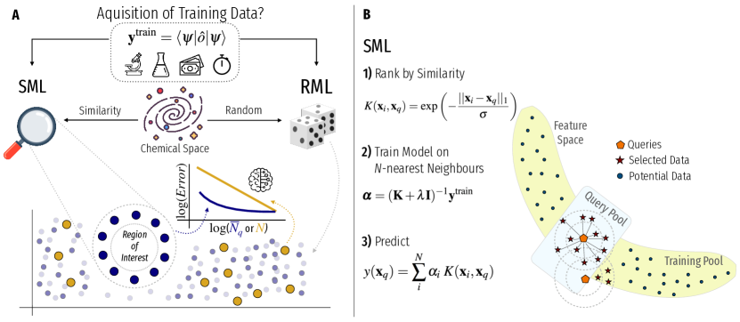
Figure 1: Schematic of similarity based machine learning (SML). (A) As a data acquisition strategy, consider similarity based vs. random selection of costly labels (y) corresponding to quantum observables and molecules (represented by wave-functions $\Psi$) from chemical space, resulting in either SML or random machine learning (RML) models, respectively. Due to SML’s exclusive focus on the region most relevant to the query improved data-efficiency is achieved, as evinced by learning curves. (B) Training procedure of SML with kernel ridge regression: Given a vast pool of potentially interesting queries (rectangle), typically only certain queries are of interest. SML selects the corresponding relevant training points ($\overline{N}_{q}$) from feature space (banana) as ranked by similarity in representation features (Step No. 1). Consequently, training SML models (Step No. 2) requires costly labels only for the $\overline{N}_{q}$ nearest neighbours (shown in circles) which do not yet overlap with any other previously selected query. Resulting query specific SML models yield similar prediction accuracy for less training data (Step No. 3).

Useful answers to experimental designfisher1936design ; chaloner1995bayesian ; pukelsheim2006optimal questions are crucial components for successful decision makingedwards1954theory ; pratt1995introduction ; berger2013statistical ; foster2021statistical ; Trommershuser2008 under finite budget and time constraints. Conventionally, optimal or near-optimal solutions are proposed by few expert scientists which severely limits humanity’s ‘experimental reach’ as high-dimensional combinatorial solution spaces pose a dramatic bottleneck. Breakthroughs in machine learning and advances in data-availability through high performance computing or high-throughput experimentation are accelerating the pace of scientific discovery and are considered by some to even represent a paradigm-shifthey2009the ; von_lilienfeld_quantum_2018 ; vonLilienfeld2020 . In particular, autonomous robotic experimentation in the chemical and biological sciences robotscientist ; automationscience ; Burger2020 ; Hse2019 ; Granda2018 ; alanbayesian revolutionizes humanity’s experimental reach through the capacity in which experiments can be executed. The synergy between machine learning, first principles simulations and experimental design facilitates data driven exploration in molecular and materials discovery through an accelerated feedback loopEAST . However, rigorous exploration algorithms are in dire need to bypass the combinatorial wall in the solution space.

With recent interests in data driven machine learning approaches surging, we have set out to investigate how to exploit modern statistical learning in order to assist with such experimental design exploration challengeNPolitis2017 ; tye2004application and decision making problemsedwards1954theory ; mldecision . A crucial success factor is the availability of accurate machine learning models, often relying on the increasingly prevalent paradigm ’the bigger the data the better’ as conveyed through large language model breakthroughs such as OpenAI’s impressive Generative Pre-trained Transformer (GPT-) 4. While GPT-4 is undoubtedly of value through its multimodal capabilities, including novel applications in chemical researchWhite2023 ; Jablonka2023 ; boiko2023emergent or few shot learning use cases, the overwhelming majority of human endeavours in research are still plagued by intense data scarcityWeinreich_2023 often with only hundreds if not only dozens of data points being available, without access to pre-trained all purpose models.

Typically, scarcity is due to high costs imposed by the acquisition of the necessary amount of data. Common examples include long simulation times in quantum chemistryheinen_machine_2020 , cost of compute to perform simulations or money and time to perform laboratory experiments. Consequently, the development of data-efficient machine learning models and training set selection schemes is crucialWen2023 ; Smith2018 ; synthtrain ; heinim3l ; zhang2019active ; zubatiuk2021development . Within the chemical sciences, a concept frequently referenced in drug discovery researchjohnson1990concepts ; OBoyle2016 ; Muratov2020 called ‘similar structure-similar property principle’ (SPP) suggests that when the query is known, machine learning models should be trained on instances similar to query, rather than on increasingly many diverse ones (Fig. 1A). Thus, within statistical learning, the training-query similarity emerges as a crucial measure of the predictive power of a model, possibly more relevant than the total quantity of data available.

Here we exploit the concept of SPP in quantum chemical machine learning through introduction of similarity based machine learning (SML) that generates tailored models for arbitrary queries, reaching meaningful prediction accuracy at only a fraction of the total training pool. Ranking prospective data based on similarity to a query, only the $\overline{N}_{q}$ nearest neighbours are chosen for training SML models (see Fig. 1B for kernel ridge regression based SML). Note that if not mentioned otherwise, $\overline{N}_{q}$ neighbours are selected by proximity rather than all $\overline{N}_{q}$ within a fixed distance radius. While conceptually similar to local learning algorithmsvapnik_local_learning such as k-nearest-neighbors or moving-least-squares, SML models achieve local neighbourhood weighting through kernel or bagged decision tree based methods. Within this work, we rely on kernel ridge regression for SML, which in combinations with a Gaussian or Laplacian kernel (Eq. 6-5) can be seen as a form of weighted nearest neighbour regression (see SI for further discussion). SML would be preferable for applications which require a) prior knowledge about the query pool, b) few queries of interest with properties that are expensive to measure, e.g. time or money, and c) that the property of interest is relatively easy to obtain for similar candidates.

In contrast to other data efficient learning schemes such as active learning, SML focuses on few queries at a time rather than training an all purpose model in an iterative fashion. Note that the smaller the number of relevant query instances, the more advantageous SML will be. However, SML can be extended to iterative active learning by using distance or density based training point selection if a multitude of queries is expected. Other data efficient learning algorithms such as transfer or few shot learning require pre-trained models, whereas SML solely relies on training points similar to a query, thereby opening the possibility of query aware few shot learning in domains with limited access to pre-trained models.

For exhaustive screening of chemical compound space, by contrast, conventionally trained random machine learning (RML) models are more appropriate. Note that within this work SML and RML are both based on kernel ridge regression, however, differ in their training data selection and applicability. As such, consider multi-objective compound design in which an RML model is used as a filter to scan vast domains of chemical spacekirkpatrick_chemical_2004 , thereby requiring a large and diverse training set in order to answer any query GmezBombarelli2016 ; Westermayr2023 . Once a candidate compound has been identified, i.e. we are aware of the query, SML can subsequently be used to provide highly accurate estimates for properties not covered by the highly general RML model.

After introducing SML in this article, we demonstrate its usefulness for two distinct applications: i) Quantum mechanics based molecular design: Statistical learning of quantum properties holds the promise to accelerate the computational materials design process via fast and accurate machine learning modelsgdml ; bartok2017 . Due to the size of chemical compound space (encompassing at least 10⁶⁰ compoundskirkpatrick_chemical_2004 ) and the computational cost of atomistic simulations (ranging from hours to monthsheinen_machine_2020 ), SML can dramatically reduce training data needs if target query compounds are known. ii) Organic synthesis planning: The bottleneck of molecular and materials discovery is amplified in experimental settings, due to large costs and the required manual labour. Additionally, compounds have to be synthesised or purchased before properties can be measured, adding to the cost-time complexity of molecular and materials design. We showcase how SML can be used to efficiently predict relevant properties for target boutique compounds without having make the expenditure necessary to acquire them.

Finally, we analyse the link between query and training data proximity, allowing to derive a relationship between the intrinsic dimensionality and volume of the feature space spanned by the training data. The results further corroborate the idea that with increasing local nearest neighbour density an decreasing fraction of the total data pool is required to converge to competitive performance.

II Results

II.1 Similarity Machine Learning

To assess the effect of the SML approach on learning, we compare learning curves for random and similarity based machine learning models applied to the analytically known harmonic oscillator and the Rosenbrock functions (Fig. 2 A and B). The SML learning curves exhibit dramatically lower offsets and faster convergence when compared to randomly selected ML (RML) models. See methods for more technical details on training and testing.

Figure 2: Left column: SML of a harmonic potential. Right column: SML of the Rosenbrock function. (A) Illustration of target functions and some random query points. (B) Learning curves showing systematic improvement with increasing training set size using RML and SML compared to k-NN baselines. Random (dashed) and grid (solid) indicate the initial training pool sampling of the function, respectively. The nullmodel corresponds to the averaged function value in training set. (C) Average number of nearest neighbours $\overline{N}_{q}$ as a function of a radius around a query for increasing total training set size $N_{max}$, drawn from respective ranges at random. (D) Intrinsic dimensionality $d_{id}$ and density of points $\rho$ for increasing $N_{max}$ (see Eq. (2)).

On average, only very few yet similar training points are necessary for SML to be competitive with the RML model trained on an order of magnitude more training points. In comparison with k-nearest neighbour (k-NN) regression, SML shows on a par performance when the training pool was grid sampled (Fig. 2 B). However, SML outperforms k-NN in randomly sampled training pool settings, suggesting robust performance even in sparsely sampled regions. As mentioned before, since SML is trained on the fly for each query, the use of SML is only advantageous if few queries are of concern. For exhaustive screening and enumeration studies, the conventional RML approach is more appropriate. We note the difference in shape of an SML curve when compared to learning curves reported in the literature. The rapid onset of convergence indicates that only a fraction of available nearest neighbours are necessary to reach the maximum predictive accuracy. Note that in the limit of maximum dataset size, the SML model’s prediction error will always converge towards the corresponding RML prediction error.

II.2 Dimensionality analysis

We have analysed the SML models throughout this paper using learning curves. The relationship between the predictive accuracy of a model and the number of training points is a fundamental concept in statistical learning. If trained properly, the learning curvecortes_learning_1994 must reflect the inverse relationship between out-of-sample prediction (test) error as a function of number of training points $N$. Note, in the case of SML based learning curves, $N$ corresponds to the number of nearest-neighbours $\overline{N}_{q}$ chosen for training. The logarithmized version of the leading error term is,

$$\log(\textrm{Error})\approx\log(a)-b~{}\log(N),$$ (1)

with the slope $b$ being related to the intrinsic dimensionality ($d_{id}$) and $a$ being related to the target similaritylearningcurve_review . For the development of data efficient machine learning models it is desirable to understand what decreases $\log(a)$ and increases $b$. Efforts in estimating and analysing the impact of $d_{id}$ have shown an inverse correlation with high model performance, implying that low $d_{id}$ data is generally easier to learndimlearning ; NEURIPS2019_cfcce062 ; DBLP:conf/iclr/PopeZAGG21 , and that compact representations suffice. In the limit of large $N$ and randomly sampled data, Eq. 1 must become linear for Gaussian Process Regressioncortes_learning_1994 as well as neural network regressorsMller1996 .

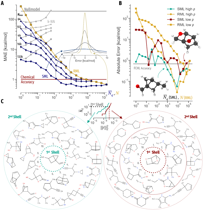
Figure 3: Training and analysis of SML models of atomization energies of QM9 ramakrishnan_quantum_2014 compounds using the FCHL19 christensen_fchl_2020 representation. (A) Learning curves for RML, SML and k-NN for increasing maximal training set sizes, drawn at random. The inset depicts the error distribution of SML models at varying training set sizes for the largest $N_{max}$. Chemical accuracy threshold shown as horizontal line. The nullmodel corresponds to the averaged function value in training set. (B) Learning curves of RML and SML models for predicting 4-methylbicyclo[2.1.0]pentane-2-carbaldehyde (https://tinyurl.com/2p9dtueh) and 3,8-dioxatricyclo[4.2.1.0^2,5]nonane (https://tinyurl.com/2p8e4d3h) with either high or low nearest neighbour density, respectively. (C) Display of the first shell (closest ten molecules) and second shell (next closest fifteen) neighbours for the two query compounds.

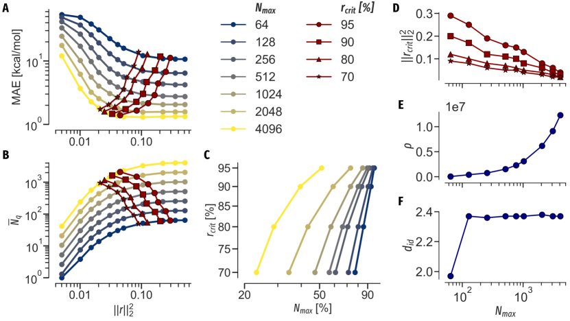
Figure 4: Distance based analysis of SML models of learning atomization energies of QM9 using FCHL19 and a Gaussian kernel. $r_{crit}$ represents the distance radius at which a certain percentage of the maximally attainable predictive accuracy is reached. (A) Systematic learning of atomization energies using only training instances within the L2-Distance specified on abscissa. (B) Averaged number of nearest neighbours around a query at different total $N_{max}$ for increasing L2-distance radius. (C) Percentage of data set size necessary to reach a certain accuracy as determined via $r_{crit}$. (D-F) $r_{crit}$, density and intrinsic dimensionality ($d_{id}$) of the QM9ramakrishnan_quantum_2014 chemical space as a function of available training points, respectively.

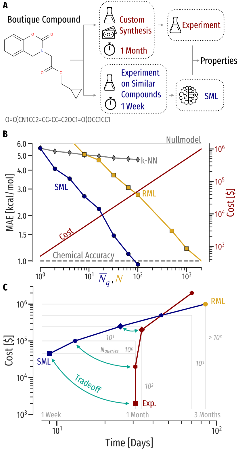
Figure 5: Example of how to use SML within a virtual custom synthesis scenario. (A) Suppose, the decision to make an investment in a certain desired boutique query compound (exemplary molecular graph and string shown as inset https://tinyurl.com/5yvxxzst) depends on a certain property. Rather than ordering a costly and time-intensive custom synthesis, one can instead simply predict the property by first ordering sufficient more easily available compounds which are similar to the query, and by subsequently measuring their properties in order to train an accurate SML model. The nullmodel corresponds to the averaged function value in training set. (B) Respective learning curves and training data acquisition cost for RML and SML models of an exemplary property (free energies of solvation) using molecules drawn at random from Enamine REAL libraries enamine_real ; enamine_realdb . Dashed horizontal line indicates chemical accuracy threshold (1 kcal/mol corresponding to experimental uncertainties in thermochemical combustion). (C) Cost vs. time associated with the generation of an SML or RML dataset ($\sim$500 US$/compound) in comparison to a ball-park synthesis cost of 2’000 US$/query for different number of queries $N_{queries}$ to be expected. The time estimate includes approximate delivery times of 5 days for SML/RML compounds and 1 month for boutique compounds, respectively, as well as an experimental throughput of 25 compounds per day.

Calculating the distances of all training points in a pool $N_{max}$ to all queries, respectively, the average amount of nearest neighbours $\overline{N}_{q}$ within a certain distance radius $r$ can be determined. Fig. 2C confirms the intuition that by increasing the total data pool $N_{max}$, the local density, i.e. the amount of neighbours within a fixed radius, grows as well. To quantify the relationship between $N_{max}$ and distance radius $r$, we use the definition of density $\rho$, i.e. $\rho=N/V=N/{r^{d_{id}}}$, with volume $V$, distance radius $r$ and intrinsic dimensionality $d_{id}$. To obtain values for $\rho$ and $d_{id}$, we transform the density equation to fit the steepest slope of $\overline{N}_{q}$ as a function of distance $r$ on a double logarithmic scale (Fig. 2C), yielding:

$$\log(N)=\log(\rho)+d_{id}~{}\log(r),$$ (2)

Fig. 2D shows the resulting density $\rho$ to increase linearly with larger pool-sizes $N_{max}$. Interestingly, our calculated $d_{id}$ effectively underestimates the respective formal dimensionality of 1D and 2D for the harmonic oscillator and Rosenbrock function (Fig. 2D). Our analysis indicates that edge artifacts introduced through the fixed function boundaries, as depicted in Fig. 2A, contribute to this effect: Queries that are close to the boundary will have less neighbours when increasing the distance radius than queries in the center, leading to an underestimated $d_{id}$ (see SI, Fig. S1). Given an infinite space and perfectly centered points, the formal $d_{id}$ can be recovered. We note that other nearest neighbour or maximum likelihood $d_{id}$ estimationsPhysRevLett.130.067401 ; Majumdar2016 ; amsaleg2015estimating ; pettis1979intrinsic are possible, but can suffer from negative bias through edge effects in higher dimensionsFacco2017 ; mle_id .

Having introduced the concept of SML and learning curves on mathematical toy functions, we will now apply SML to learning quantum properties of chemical compounds.

II.3 Quantum mechanics based virtual compound design

To illustrate a meaningful use-case of SML, consider a typical problem of computational molecular and materials design: Organic light-emitting diodes. Consider furthermore that a promising compound would have been identified through sophisticated screening of a very large set of potential candidate compounds. Suppose that the screening imposes all necessary constraints on the candidate compound, except for quantum mechanics based excited states calculations which is not only difficult to model, but is also computationally expensive for larger compoundsWestermayr2020 ; Westermayr2021 . In this scenario, it is difficult to make a rational decision due to the high computational cost and time required to perform the quantum calculation. Furthermore, given the scarcity of literature excited states data throughout chemical compound space, RML models such as state of the art neural network architecturespmlr-v139-satorras21a ; Atz2022 ; EquiformerV2 ; 2022equivariant in quantum chemistry would potentially require larger volumes of data to yield accurate estimates. By contrast, due to its data-efficiency, SML will be able to produce substantially more accurate predictions after training on substantially less data.

Obviously, this molecular design scenario is not restricted to organic electronics. As a numerical illustration, we report the application of SML to learning quantum mechanics based calculated atomization energies (rather than excited states) of organic molecules, as reported in the QM9ramakrishnan_quantum_2014 dataset, rather than for organic materials candidates. As for the harmonic oscillator and Rosenbrock function discussed above, Fig. 3A displays overwhelming numerical evidence that SML models also exhibit superior data-efficiency when it comes to molecules and their properties. More specifically, for all tested $N_{max}$, SML learning curves exhibit a much reduced offset, and converge to the accuracy of the RML learning curve at $N_{max}$ for training set sizes that are smaller by orders of magnitude. In contrast, k-NN did not improve beyond the first neighbour. Note also the robustness of SML: As the number of nearest neighbours $\overline{N}_{q}$ grows, its predictive variance decreases systematically (Fig. 3A inset). Furthermore, SML performs consistently when applied to quantum properties in chemical compound space as datasets and molecular representations are being varied (for further examples see SI and Fig. S3).

At increasingly large $N_{max}$, a shoulder becomes apparent for small training set sizes with less than $\overline{N}_{q}$=30. Moreover, the larger $N_{max}$, the more data-efficient the SML model (earlier flattening) suggesting that the increase in local neighbour density leads to faster saturation in learning (see II. B for in-depth dimensionality analysis in analogy to the harmonic oscillator and Rosenbrock function). At the largest $N_{max}$ possible within the QM9 data-set ($\sim$134k molecules for training), SML reaches the coveted chemical accuracy of on average 1 kcal/mol at only 100 training points for any given query. For RML models, this would have solved the ’QM9-IPAM-Challenge’ in quantum chemical machine learningvonLilienfeldburke2020 ; von_lilienfeld_exploring_2020 . Note that many applications in quantum mechanics based simulation of molecules and materials are rather concerned with few queries than many. This indicates, that SML might be the superior choice, than learning a general purpose property throughout chemical compound space, such as a universal force field.

To illustrate the effect of the query-specific density on the SML model, we compare two query compounds with respectively low and high density of neighbours in chemical space. More specifically, we consider the caged ether-bridged C₆H₈O₂ compound, 3,8-dioxatricyclo[4.2.1.0^2,5]nonaneSTOUT ; leruli , and the fused C₇H₁₀O aldehyde, 4-methylbicyclo[2.1.0]pentane-2-carbaldehydeSTOUT ; leruli , encoding motifs that are respectively rather rare or frequent within the chemical space spanned by QM9ramakrishnan_quantum_2014 . SML learning curves (Fig. 3B) confirm the expectation: The higher the density of neighbours the better the learning curve’s off-set and slope in the low-data limit. Note that for query specific training resulting learning curves can also increase with training set size. This is in stark contrast to the statistical learning tenet that averaged prediction errors must decay systematically cortes_learning_1994 ; Mller1996 . Visual inspection of the closest nearest neighbours in terms of FCHL based distances (Fig. 3C) shows barely any relative chemical trends of similarity. Using BoB based distances, however, the visual inspection is more straightforward: Fig. S5 reveals for example that for a high-density query a tautomer in QM9 got selected by SML, resulting in near-perfect predictions.

II.4 Dimensionality analysis of QM9

To gain a better understanding of the relation between query and training data proximity, SML models have been trained - similar as reported for the harmonic oscillator and Rosenbrock function - using an increasing distance radius as a measure to select training data. Fig. 4A indicates that with increasing $N_{max}$ the distance radius required to reach the final accuracy becomes smaller. Concurrently, the average amount of nearest neighbours $\overline{N}_{q}$ in a smaller radius also increases (Fig. 4B). We define a critical radius $r_{crit}$ to determine the distance cutoff at which 70, 80, 90, 95% of the maximum accuracy is reached at each $N_{max}$ (Fig. 4A), respectively. We observe that at increasing $N_{max}$, $r_{crit}$ becomes smaller (Fig. 4D). Calculating the average amount of neighbours $\overline{N}_{q}$ within $r_{crit}$ (Fig. 4B), a pareto front becomes apparent, confirming that at increasing $N_{max}$ a fraction of the data is sufficient (Fig. 4C). We apply Eq. 2 on Fig.4B to obtain the density $\rho$ and $d_{id}$. As expected, the density $\rho$ increases with $N_{max}$ (Fig. 4E). However, in consideration of the size of chemical compound space and ways of systematic enumeration, it is unclear how and if the density will converge and how this will influence the learning of properties in chemical compound space. The estimated $d_{id}$ converges to a value of 2.4 for $N_{max}>$ $\sim$100 using a Gaussian kernel (Fig. 4F) and 1.7 using a Laplacian kernel (see SI Fig. S11). While estimates of the $d_{id}$ for popular chemical datasets have not been rigorously reported yet, we note that the $d_{id}$ of a fixed segment of chemical compound space is bound to an upper limit of 4$N$-6 when using a roto-translational invariant representation. Reasons for potential underestimates can be finite boundaries in terms of representation or even chemical space. Points in high dimensions tend to be localized at the surface of the hypersphere. The effect of edge artifacts can further be amplified through the high dimensionality of molecular representation, which typically are vectors containing thousands of entries. However, we report that even a high dimensional representation such as BoB ($\sim$1’000 entries for QM9) shows high co-linearity compared to uniform random vectors of the same size (see SI Fig. S12).

II.5 Organic synthesis planning

A SML use-case in the context of managing synthesis planningMolga2021 ; Coley2018 ; Levin2022 ; MikulakKlucznik2020 within industrial chemistry could be as follows: Consider the problem of acquiring non-trivial molecular properties of one boutique compound through experimental measurements. Synthesis of the compound prior to measurements is also assumed to first require substantial experimental efforts resulting in very long delivery times (also known as ’lead times’)Hughes2011 . Note that this is not an unusual ’academic’ situation as the latter can nowadays be performed commercially through synthesis service companies such as Enamine Ltd. While such services have reached considerable reliability, reporting success rates of 60-80% and higher, challenging boutique target compounds, for example cyclopropylmethyl2-(2-oxo-3,4-dihydro-2H-1,3-benzoxazin-3-yl)acetateSTOUT ; leruli on display in Fig. 5A can impose substantial time delays until the compound has been made, characterized, and shipped, increasing lead times to several weeks or more. Alternatively, SML can be used to make accurate property predictions, rather than measurements, before having to wait out the lead time and measuring the target compound’s properties: First ordering and measuring the most similar compounds with much reduced lead times, for example readily deliverable (3-5 days) building blocks from the Enamine REAL libraryenamine_real ; enamine_realdb used for the synthesis of our exemplary boutique compound, would allow for rapidly making the measurements to generate the training data for subsequent SML model generation. The resulting SML models can then be used to accurately infer the property for the original boutique target compound. In comparison to the naive approach of simply waiting for the compound to be delivered, followed by measurements of the properties, this procedure would effectively enable a dramatic cut down of the time to decision while keeping the financial burden for data acquisition at a minimum.

To numerically illustrate the application of SML towards such use cases, we have relied on the aforementioned specific example product (cyclopropylmethyl2-(2-oxo-3,4-dihydro-2H-1,3-benzoxazin-3-yl)acetate), as well as 999 other boutique molecules (see data availability section for a complete list) with lead times of 3 to 4 weeks on average. As a relevant property, we have selected calculated free energy of solvation estimatesRMG ; RMG2 as a proxy to the measurement. As to be expected from our discussions in the preceding sections, resulting learning curves suggest that on average SML requires a magnitude less data than RML and, similarly, outperforms k-NN (Fig. 5B). Assuming a 500 US$/compound price level on average, estimated purchasing costs for training data-acquisition are shown, also indicating substantial potential for savings, i.e. time is money.

Given that there are multiple queries (up to 1’000), we have also assessed to which degree SML can benefit from synergies due to overlapping nearest neighbours of distinct queries. This possibility would reduce the scaling from the worst case upper bound imposed by RML, rendering SML preferable in terms of time and cost for larger numbers of target queries. To illustrate this scenario, and without loss of generality, we define the target accuracy to correspond to chemical accuracy (1 kcal/mol). Assuming up to 1’000 queries, we have applied SML to select a jointly combined training set containing the closest nearest neighbours of the selected queries. Analysis of the $N_{neighs}$ required per query to reach 1 kcal/mol (see SI), indicates that less $N_{neighs}$ are required when considering shared neighbourhood SML models, rather than single query SML. Note that with increasing $N_{queries}$, also increasingly larger SML training set is required, ultimately converging to the upper bound used within RML models. Thus, variety in the query-set also requires variety training set, whereas few queries are more efficiently predicted via SML.

Additionally, time and cost are constraints to be considered during the design process (Fig. 5C). Albeit the data-acquisition costs of machine learning approaches can be more costly than directly ordering the target compounds (we assume 2’000 US$/target compound price in Fig.5C), SML and RML can become financially advantageous for large sets of $N_{queries}$. For a modest number of expected queries, SML will be preferable, whereas for many queries RML is the method of choice. In our example, however, the cost per query has not been included as an additional constraint when selecting nearest neighbours. This could lower the total cost even further. In terms of time to decision, SML will always be preferable. Note that the specific variables cost and time strongly depend on each scenario. In conclusion, given additional constraints and a large chemical space to choose from, approximate nearest neighbour selectionann is beneficial for reducing cost and time to decision in planning the management of chemical synthesis.

II.6 Limitations

We want to note that any limitations that apply to an RML model will also apply to SML since both only differ in their training data, but not in their underlying machine learning algorithm, e.g. kernel ridge regression. Since the choice of representation and distance metric influences the choice of nearest neighbours, an improvement in both, e.g. by including more physical knowledge or metric learningFabregat2022 , will result in lower learning curve offsets (see SI Fig. S3). Conversely, low local nearest neighbour density (Fig.3B) will require more data in order to reach optimal accuracy. Additionally, the compute time for an exact nearest neighbour search grows linearly with $O(n)$. However, since the local nearest neighbour density is proportional to the size of search space (see Fig. 4), the $O(\log{}n)$ scaling of approximate nearest neighbour algorithms, commonly used with millions of data points, becomes more effective. Further strategies could encompass to use efficient low dimensional representations for approximate nearest neighbour searches while using higher quality representations for regression, resulting in a time vs. accuracy trade-off. To make the most out of SML within multi query scenarios, it is recommended to maximize the overlap of shared SML training sets as described in the supplementary information. Methods such as Auto3Dauto3d , OQMLheini_geom , Graph-To-StructureLemm2021 or generative modelspmlr-v162-hoogeboom22a ; pmlr-v202-xu23n ; jing2022torsional could further facilitate the generation of 3D input structures for quantum chemistry based models to avoid performance loss by using lower levels of theory geometries such as from force fieldsVazquezSalazar2021 . Additionally, the atoms-in-moleculeAMONS (AMONS) approach could further aid the applicability of SML by using smaller molecular building blocks to predict significantly larger query compounds.

III Discussion

We have presented numerical evidence that similarity based machine learning (SML), an approach to select data and train a model on-the-fly for specific queries, can offer substantial improvements in data efficiency for certain use-cases. Applying SML to problems in quantum mechanics and organic synthesis planning, we have found dramatically lower offsets in learning curvescortes_learning_1994 , enabling meaningful decision making at a fraction of the total training set size. Comparisons of SML with other similarity based methods indicate robust performance, even in high dimensional feature spaces. Large training set sizes and associated costs of data acquisition render the use of one-fits-all ML models unfeasible related to the size of chemical compound space. The shape of SML learning curves suggest meaningful deviations from ’the bigger the better’ paradigm indicating that learning is rather dominated by locality effects, and even saturates upon inclusion of sufficiently many nearest neighbours in training.

After introducing and demonstrating SML for harmonic oscillator and Rosenbrock functions, we have demonstrated its usefulness for quantum mechanics based molecular design where we can reach the coveted 1 kcal/mol chemical accuracy already after just 100 nearest neighbours. This kind of task requires conventional RML models to be trained on thousands of data points. More fundamentally, however, we have derived a relationship between the intrinsic dimensionality and volume of the feature space spanned by the training data which governs the overall model accuracy. In managing the planning of experimental organic synthesis projects, we have shown that SML can bypass time intensive custom synthesis by using readily available compounds similar to the boutique compounds of interest.

We believe that for certain decision problems in chemistry the paradigm of ’the bigger the data the better’ is not optimal, and that tailored, query specific SML models reach predictive power already for training set sizes that are orders of magnitude smaller than for conventional RML models. More generally, we expect SML to be advantageous for any problem with a) prior knowledge of and access to molecular features in query pool (to easily calculate similarity), b) few queries of interest with labels that are expensive to measure (e.g. long computation times or high costs) c) labels for similar candidates in pool that are less difficult to obtain. Moreover, the implicitly defined domain of applicability of the model provides an indication for the reliability of a machine learning model for unseen queries and inherently limits the usefulness outside of this domain (extrapolationextrapol_ml ). Potential applications beyond chemistry could include predictive maintenance tasks in computer aided infrastructurematerialsdegrad or aerospace engineeringaviation1 ; aviation2 . Future work will address, automated experimental design, deriving ready made models in quantum chemistry or multilevel learning, improving similarity measurements, as well as exploring fast and approximate neighbour searches (cf. turbo similarity fusion)Fabregat2022 ; Gardiner2009 ; MirandaQuintana2021-1 ; MirandaQuintana2021-2 .

IV Methods

IV.1 Kernel Ridge Regression (KRR)

We rely on kernel ridge regression (KRR)krige_statistical_1951 due to its successes in small data scenarios, however, other machine learning regressors are possible. Kernel based methods belong to the class of supervised machine learning models and are – despite their simplicity – a powerful approach for learning molecules and materials properties. In ridge regression, a mapping function is learned, relating a representation vector x to a label $y$krige_statistical_1951 ; vapnik_nature_2000 . The ’kernel trick’ renders the problem linear through the use of kernel functions that yield the inner product of high dimensional representations x. In practice, KRR is formulated as follows:

$$y(\textbf{x}_{q})=\sum^{N}_{i}\alpha_{i}\;K(\textbf{x}_{i},\textbf{x}_{q})$$ (3)

with $\alpha_{i}$ being the regression coefficient, $\textbf{x}_{i}$ being the i-th representation vector of the training set, $\textbf{x}_{q}$ being the query representation and kernel function $K$. The regression coefficients $\alpha$ are calculated through a closed-form solution:

$$\bm{\alpha}=(\textbf{K}+\lambda\textbf{I})^{-1}\textbf{y}^{\textrm{train}}$$ (4)

with the identity matrix I and a regularization coefficient $\lambda$. The latter depends on the anticipated noise in the input and labels and has to be determined through hyperparameter optimization.

IV.2 Kernel Functions

As a similarity measure, the Laplacian (Eq. 5) and Gaussian (Eq. 6) kernels are the most common choices.

$$K(\textbf{x}_{i},\textbf{x}_{q})=\exp\left(-\frac{||\textbf{x}_{i}-\textbf{x}_{q}||_{1}}{\sigma}\right)$$ (5)

$$K(\textbf{x}_{i},\textbf{x}_{q})=\exp\left(-\frac{||\textbf{x}_{i}-\textbf{x}_{q}||^{2}_{2}}{2\sigma^{2}}\right)$$ (6)

with $\sigma$ being the kernel width, an additional hyperparameter to optimize. The kernel function for local atomic representations can be rewritten as the sum of pair-wise kernels:

$$K_{iq}=\sum_{I\in i}\sum_{J\in q}\;K(\textbf{x}_{I},\textbf{x}_{J})$$ (7)

with $I$ and $J$ being atoms in the training and query, respectively. Kernels for local atomic representations of molecules are often augmented with an additional elemental screening function to compare only atoms of the same nuclear charge:

$$K(\textbf{x}_{I},\textbf{x}_{J})=\delta_{Z_{I},Z_{J}}\exp\left(-\frac{||\textbf{x}_{I}-\textbf{x}_{J}||^{2}_{2}}{2\sigma^{2}}\right)$$ (8)

with Kronecker Delta $\delta$, nuclear charges $Z$ and atomic representations x. In order to use local representations as a normalized molecular similarity measure, Eq.8 can be expressed as the sum of local atomic comparisons:

$$d_{\textrm{global}}(\textbf{x}_{i},\textbf{x}_{q})=\delta_{Z_{I},Z_{J}}\sum_{I\in i}\sum_{J\in q}\textbf{x}_{I}\cdot\textbf{x}_{J}$$ (9)

$$K(\textbf{x}_{i},\textbf{x}_{q})=\exp\left(-\frac{d(\textbf{x}_{i},\textbf{x}_{i})-2~{}d(\textbf{x}_{i},\textbf{x}_{q})+d(\textbf{x}_{q},\textbf{x}_{q}))}{2\sigma^{2}}\right)$$ (10)

IV.3 Representations

We use standard representations which have been developed, benchmarked and continuously improved over the past years for learning quantum properties. The Coulomb Matrix (CMrupp_fast_2012 ) contains a 1-body self interaction and a 2-body Coulomb repulsion term and has been one of the first representations developed for machine learning quantum properties. The bag-of-bonds (BoBhansen_machine_2015 ) representation, the direct successor of the CM, vectorizes the CM terms into fixed size bins, thus enabling the strict comparison between chemically similar environments. The spectrum of London and Axilrod–Teller–Muto (SLATMAMONS ) representation uses London dispersion contributions as the 2-body and the Axilrod–Teller–Muto potential as the 3-body term and has shown improved performance over BoB for learning quantum properties. The Faber–Christensen–Huang–Lilienfeld (FCHL19christensen_fchl_2020 ) representation describes a local atomic environment per atom, respectively, and contains 2 and 3-body terms similar to Behler & Parrinello atomic symmetry functions (ACSFbehler_atom-centered_2011 ) accounting for distance and angular information. We used the optimized FCHL19 parameters as recommended in Ref.christensen_fchl_2020 . The Smooth Overlap of Atomic Positions (SOAP)SOAP representation is, similar to FCHL19, a local atomic representation that encodes local geometries through spherical harmonics and radial basis functions. We used $n_{max}=3$ and $l_{max}=5$ with $\sigma=0.1$ and a cutoff of 3.5 $\mathrm{\SIUnitSymbolAngstrom}$ as SOAP settings. For the learning of the free energy of solvation, we used FCHL19 and the free-energy-machine-learning (FML) schemeWeinreich2021 .

IV.4 Training

We optimize the hyperparameters $\sigma$ and $\lambda$ through cross-validation on the largest training set size. Both parameters are held constant for all other training set sizes. To train an SML model, the pair-wise distances of a query to all available datapoints defined by $N_{max}$ are calculated. An overview of training/query set sizes and distance metrics for each representation and dataset can be seen in Tab. S1 in the SI. After sorting all points by distance, only the $\overline{N}_{q}$ closest neighbours are considered for training. SML learning curve are obtained by averaging across all single query runs. Similarly, k-NN baselines are calculated by averaging the labels of the closest $\overline{N}_{q}$ neighbours weighted by the distance to the query, respectively. RML models are trained choosing $N$ data points at random. The regression coefficients are obtained through Eq.4 and the query label predicted via Eq.3 (Fig. 1 B). Note, RML models are only trained once to predict the labels of all queries, whereas SML and k-NN models are trained on-the-fly for each query, respectively.

IV.5 Data

To assess SML, several quantum based datasets have been considered. The QM7 dataset totals 7’165 organic molecules up to seven heavy atoms (CONS)rupp_fast_2012 ; blum_970_2009 . Atomization energies and structures were calculated using the Perdew-Burke-Ernzerhof hybrid functional (PBE0) level of quantum chemistryrupp_fast_2012 ; blum_970_2009 . The QM9ramakrishnan_quantum_2014 dataset is a hallmark benchmark in quantum machine learning. Containing 133’885 small organic molecules up to nine heavy atoms (CONF), properties were calculated at the B3LYP/6-31G(2df,p) level of quantum chemistryramakrishnan_quantum_2014 . Additionally, a subset of 6’095 C₇O₂H₁₀ constitutional isomers has been used as a toy case.

The Enamine REAL database is the largest enumerated database of synthetically available compounds containing over 4.5 billion moleculesenamine_real ; enamine_realdb . We have chosen 1’000 random query compounds of the REAL library containing 6-21 heavy atoms. For training, we used the Enamine REAL building blocks, which encompass over 128’856 compounds that are used to synthesize the Enamine REAL dataset. We applied a SMILESweininger_smiles_1988 standardization protocol and filtered all compounds containing B, Si or Sn elements, yielding a total number of 124’440 compounds. 3D coordinates and conformers for all compounds were generated with ETKDGriniker_better_2015 . A maximum of 25 conformers were further relaxed using GFN2-xTBbannwarth_gfn2-xtbaccurate_2019 and corresponding Boltzmann weights obtained through energy rankings. As a training label, free energies of solvation were computed using the Reaction-Mechanism-GeneratorRMG ; RMG2 .

V Acknowledgement

Icons used in Figures 1,5 and S16. were created by Freepik, photo3idea_studio, Victoruler, Maxim Basinski Premium and Monkik of flaticon.com. This project has received funding from the European Research Council (ERC) under the European Union’s Horizon 2020 research and innovation programme (grant agreement No. 772834). This research is part of the University of Toronto’s Acceleration Consortium, which receives funding from the Canada First Research Excellence Fund (CFREF). Part of this research was performed while GFvR was visiting the Institute for Pure and Applied Mathematics (IPAM), which is supported by the National Science Foundation (Grant No. DMS-1925919).

VI Author Contributions

DL wrote new software used in the work, produced all figures, performed the literature search, compiled the references. DL and GvR acquired the data. DL, GvR and OAvL conceived and planned the project, analyzed and interpreted the results, and wrote the manuscript.

VII Data and Code Availability

The QM9 dataset is available at https://dx.doi.org/10.6084/m9.figshare.c.978904.v5. The QM7 dataset is available at http://quantum-machine.org/datasets/. The Enamine REAL database and building blocks can be accessed at https://enamine.net/compound-collections/real-compounds/real-database. The code to produce SML learning curves is available at https://doi.org/10.5281/zenodo.7870923.

VIII Conflict of Interest

The authors have no conflict of interest.

IX References

References

- (1) R. A. Fisher, “Design of experiments,” British Medical Journal, vol. 1, no. 3923, p. 554, 1936.
- (2) K. Chaloner and I. Verdinelli, “Bayesian experimental design: A review,” Statistical science, pp. 273–304, 1995.
- (3) F. Pukelsheim, Optimal design of experiments. SIAM, 2006.
- (4) W. Edwards, “The theory of decision making.,” Psychological bulletin, vol. 51, no. 4, p. 380, 1954.
- (5) J. W. Pratt, H. Raiffa, and R. Schlaifer, Introduction to statistical decision theory. MIT press, 1995.
- (6) J. O. Berger, Statistical decision theory and Bayesian analysis. Springer Science & Business Media, 2013.
- (7) D. J. Foster, S. M. Kakade, J. Qian, and A. Rakhlin, “The statistical complexity of interactive decision making,” arXiv preprint arXiv:2112.13487, 2021.
- (8) J. Trommershäuser, L. T. Maloney, and M. S. Landy, “Decision making, movement planning and statistical decision theory,” Trends in Cognitive Sciences, vol. 12, pp. 291–297, Aug. 2008.
- (9) T. Hey, S. Tansley, and K. Tolle, The Fourth Paradigm: Data-Intensive Scientific Discovery. Microsoft Research, October 2009.
- (10) O. A. von Lilienfeld, “Quantum Machine Learning in Chemical Compound Space,” Angewandte Chemie International Edition, vol. 57, pp. 4164–4169, Apr. 2018.
- (11) O. A. von Lilienfeld, “Introducing machine learning: Science and technology,” Machine Learning: Science and Technology, vol. 1, p. 010201, Feb. 2020.
- (12) R. D. King, K. E. Whelan, F. M. Jones, P. G. K. Reiser, C. H. Bryant, S. H. Muggleton, D. B. Kell, and S. G. Oliver, “Functional genomic hypothesis generation and experimentation by a robot scientist,” Nature, vol. 427, pp. 247–252, Jan. 2004.
- (13) R. D. King, J. Rowland, S. G. Oliver, M. Young, W. Aubrey, E. Byrne, M. Liakata, M. Markham, P. Pir, L. N. Soldatova, A. Sparkes, K. E. Whelan, and A. Clare, “The automation of science,” Science, vol. 324, pp. 85–89, Apr. 2009.
- (14) B. Burger, P. M. Maffettone, V. V. Gusev, C. M. Aitchison, Y. Bai, X. Wang, X. Li, B. M. Alston, B. Li, R. Clowes, N. Rankin, B. Harris, R. S. Sprick, and A. I. Cooper, “A mobile robotic chemist,” Nature, vol. 583, pp. 237–241, July 2020.
- (15) F. Häse, L. M. Roch, and A. Aspuru-Guzik, “Next-generation experimentation with self-driving laboratories,” Trends in Chemistry, vol. 1, pp. 282–291, June 2019.
- (16) J. M. Granda, L. Donina, V. Dragone, D.-L. Long, and L. Cronin, “Controlling an organic synthesis robot with machine learning to search for new reactivity,” Nature, vol. 559, pp. 377–381, July 2018.
- (17) R. J. Hickman, M. Aldeghi, F. Häse, and A. Aspuru-Guzik, “Bayesian optimization with known experimental and design constraints for chemistry applications,” Digital Discovery, vol. 1, pp. 732–744, 2022.
- (18) B. Huang, G. F. von Rudorff, and O. A. von Lilienfeld, “The central role of density functional theory in the AI age,” Science, vol. 381, pp. 170–175, July 2023.
- (19) S. N. Politis, P. Colombo, G. Colombo, and D. M. Rekkas, “Design of experiments (DoE) in pharmaceutical development,” Drug Development and Industrial Pharmacy, vol. 43, pp. 889–901, Feb. 2017.
- (20) H. Tye, “Application of statistical ‘design of experiments’ methods in drug discovery,” Drug discovery today, vol. 9, no. 11, pp. 485–491, 2004.
- (21) D. Haussler, “Decision theoretic generalizations of the pac model for neural net and other learning applications,” in The Mathematics of Generalization, pp. 37–116, CRC Press, 2018.
- (22) A. D. White, “The future of chemistry is language,” Nature Reviews Chemistry, vol. 7, pp. 457–458, May 2023.
- (23) K. M. Jablonka, P. Schwaller, A. Ortega-Guerrero, and B. Smit, “Is GPT-3 all you need for low-data discovery in chemistry?,” Chemrxiv, Feb. 2023.
- (24) D. A. Boiko, R. MacKnight, and G. Gomes, “Emergent autonomous scientific research capabilities of large language models,” arXiv preprint arXiv:2304.05332, 2023.
- (25) J. Weinreich, G. F. von Rudorff, and O. A. von Lilienfeld, “Encrypted machine learning of molecular quantum properties,” Machine Learning: Science and Technology, vol. 4, p. 025017, apr 2023.
- (26) S. Heinen, M. Schwilk, G. F. v. Rudorff, and O. A. v. Lilienfeld, “Machine learning the computational cost of quantum chemistry,” Machine Learning: Science and Technology, vol. 1, p. 025002, Mar. 2020. Publisher: IOP Publishing.
- (27) Y. Wen, Z. Li, Y. Xiang, and D. Reker, “Improving molecular machine learning through adaptive subsampling with active learning,” Digital Discovery, vol. 2, no. 4, pp. 1134–1142, 2023.
- (28) J. S. Smith, B. Nebgen, N. Lubbers, O. Isayev, and A. E. Roitberg, “Less is more: Sampling chemical space with active learning,” The Journal of Chemical Physics, vol. 148, May 2018.
- (29) J. L. A. Gardner, K. T. Baker, and V. L. Deringer, “Synthetic pre-training for neural-network interatomic potentials,” arXiv, 2023.
- (30) S. Heinen, D. Khan, G. F. von Rudorff, K. Karandashev, D. J. A. Arrieta, A. J. A. Price, S. Nandi, A. Bhowmik, K. Hermansson, and O. A. von Lilienfeld, “Reducing training data needs with minimal multilevel machine learning (m3l),” arXiv, 2023.
- (31) L. Zhang, D.-Y. Lin, H. Wang, R. Car, and E. Weinan, “Active learning of uniformly accurate interatomic potentials for materials simulation,” Physical Review Materials, vol. 3, no. 2, p. 023804, 2019.
- (32) T. Zubatiuk and O. Isayev, “Development of multimodal machine learning potentials: Toward a physics-aware artificial intelligence,” Accounts of Chemical Research, vol. 54, no. 7, pp. 1575–1585, 2021.
- (33) M. A. Johnson and G. M. Maggiora, Concepts and applications of molecular similarity. Wiley, 1990.
- (34) N. M. O’Boyle and R. A. Sayle, “Comparing structural fingerprints using a literature-based similarity benchmark,” Journal of Cheminformatics, vol. 8, July 2016.
- (35) E. N. Muratov, J. Bajorath, R. P. Sheridan, I. V. Tetko, D. Filimonov, V. Poroikov, T. I. Oprea, I. I. Baskin, A. Varnek, A. Roitberg, O. Isayev, S. Curtalolo, D. Fourches, Y. Cohen, A. Aspuru-Guzik, D. A. Winkler, D. Agrafiotis, A. Cherkasov, and A. Tropsha, “QSAR without borders,” Chemical Society Reviews, vol. 49, no. 11, pp. 3525–3564, 2020.
- (36) L. Bottou and V. Vapnik, “Local Learning Algorithms,” Neural Computation, vol. 4, pp. 888–900, 11 1992.
- (37) P. Kirkpatrick and C. Ellis, “Chemical space,” Nature, vol. 432, pp. 823–823, Dec. 2004. Number: 7019 Publisher: Nature Publishing Group.
- (38) R. Gómez-Bombarelli, J. Aguilera-Iparraguirre, T. D. Hirzel, D. Duvenaud, D. Maclaurin, M. A. Blood-Forsythe, H. S. Chae, M. Einzinger, D.-G. Ha, T. Wu, G. Markopoulos, S. Jeon, H. Kang, H. Miyazaki, M. Numata, S. Kim, W. Huang, S. I. Hong, M. Baldo, R. P. Adams, and A. Aspuru-Guzik, “Design of efficient molecular organic light-emitting diodes by a high-throughput virtual screening and experimental approach,” Nature Materials, vol. 15, pp. 1120–1127, Aug. 2016.
- (39) J. Westermayr, J. Gilkes, R. Barrett, and R. J. Maurer, “High-throughput property-driven generative design of functional organic molecules,” Nature Computational Science, vol. 3, pp. 139–148, Feb. 2023.
- (40) S. Chmiela, A. Tkatchenko, H. E. Sauceda, I. Poltavsky, K. T. Schütt, and K.-R. Müller, “Machine learning of accurate energy-conserving molecular force fields,” Science Advances, vol. 3, May 2017.
- (41) A. P. Bartók, S. De, C. Poelking, N. Bernstein, J. R. Kermode, G. Csányi, and M. Ceriotti, “Machine learning unifies the modeling of materials and molecules,” Science Advances, vol. 3, no. 12, p. e1701816, 2017.
- (42) C. Cortes, L. D. Jackel, S. A. Solla, V. Vapnik, and J. S. Denker, “Learning Curves: Asymptotic Values and Rate of Convergence,” in Advances in Neural Information Processing Systems 6 (J. D. Cowan, G. Tesauro, and J. Alspector, eds.), pp. 327–334, Morgan-Kaufmann, 1994.
- (43) T. Viering and M. Loog, “The shape of learning curves: a review,” 2021. arXiv:2103.10948.
- (44) P. Pope, C. Zhu, A. Abdelkader, M. Goldblum, and T. Goldstein, “The intrinsic dimension of images and its impact on learning,” 2021. arXiv:2104.08894.
- (45) A. Ansuini, A. Laio, J. H. Macke, and D. Zoccolan, “Intrinsic dimension of data representations in deep neural networks,” in Advances in Neural Information Processing Systems (H. Wallach, H. Larochelle, A. Beygelzimer, F. d'Alché-Buc, E. Fox, and R. Garnett, eds.), vol. 32, Curran Associates, Inc., 2019.
- (46) P. Pope, C. Zhu, A. Abdelkader, M. Goldblum, and T. Goldstein, “The intrinsic dimension of images and its impact on learning,” in 9th International Conference on Learning Representations, ICLR 2021, Virtual Event, Austria, May 3-7, 2021, OpenReview.net, 2021.
- (47) K.-R. Müller, M. Finke, N. Murata, K. Schulten, and S. Amari, “A numerical study on learning curves in stochastic multilayer feedforward networks,” Neural Computation, vol. 8, pp. 1085–1106, July 1996.
- (48) R. Ramakrishnan, P. O. Dral, M. Rupp, and O. A. von Lilienfeld, “Quantum chemistry structures and properties of 134 kilo molecules,” Scientific Data, vol. 1, pp. 1–7, Aug. 2014. Number: 1 Publisher: Nature Publishing Group.
- (49) A. S. Christensen, L. A. Bratholm, F. A. Faber, and O. Anatole von Lilienfeld, “FCHL revisited: Faster and more accurate quantum machine learning,” The Journal of Chemical Physics, vol. 152, p. 044107, Jan. 2020. Publisher: American Institute of Physics.
- (50) “Real compounds (enamine, 2022); https://enamine.net/compound-collections/real-compounds.”
- (51) “Real database (enamine, 2022); https://enamine.net/compound-collections/real-compounds/real-database.”
- (52) I. Macocco, A. Glielmo, J. Grilli, and A. Laio, “Intrinsic dimension estimation for discrete metrics,” Phys. Rev. Lett., vol. 130, p. 067401, Feb 2023.
- (53) S. Majumdar and S. Basak, “Exploring intrinsic dimensionality of chemical spaces for robust QSAR model development: A comparison of several statistical approaches,” Current Computer Aided-Drug Design, vol. 12, pp. 294–301, Oct. 2016.
- (54) L. Amsaleg, O. Chelly, T. Furon, S. Girard, M. E. Houle, K.-i. Kawarabayashi, and M. Nett, “Estimating local intrinsic dimensionality,” in Proceedings of the 21th ACM SIGKDD International Conference on Knowledge Discovery and Data Mining, pp. 29–38, 2015.
- (55) K. W. Pettis, T. A. Bailey, A. K. Jain, and R. C. Dubes, “An intrinsic dimensionality estimator from near-neighbor information,” IEEE Transactions on pattern analysis and machine intelligence, no. 1, pp. 25–37, 1979.
- (56) E. Facco, M. d’Errico, A. Rodriguez, and A. Laio, “Estimating the intrinsic dimension of datasets by a minimal neighborhood information,” Scientific Reports, vol. 7, Sept. 2017.
- (57) E. Levina and P. Bickel, “Maximum likelihood estimation of intrinsic dimension,” in Advances in Neural Information Processing Systems (L. Saul, Y. Weiss, and L. Bottou, eds.), vol. 17, MIT Press, 2004.
- (58) J. Westermayr, M. Gastegger, and P. Marquetand, “Combining SchNet and SHARC: The SchNarc machine learning approach for excited-state dynamics,” The Journal of Physical Chemistry Letters, vol. 11, pp. 3828–3834, Apr. 2020.
- (59) J. Westermayr and P. Marquetand, “Machine learning for electronically excited states of molecules,” Chemical Reviews, vol. 121, pp. 9873–9926, Nov. 2020.
- (60) V. G. Satorras, E. Hoogeboom, and M. Welling, “E(n) equivariant graph neural networks,” in Proceedings of the 38th International Conference on Machine Learning (M. Meila and T. Zhang, eds.), vol. 139 of Proceedings of Machine Learning Research, pp. 9323–9332, PMLR, 18–24 Jul 2021.
- (61) K. Atz, C. Isert, M. N. A. Böcker, J. Jiménez-Luna, and G. Schneider, “-quantum machine-learning for medicinal chemistry,” Physical Chemistry Chemical Physics, vol. 24, no. 18, pp. 10775–10783, 2022.
- (62) Y.-L. Liao, B. Wood, A. Das, and T. Smidt, “Equiformerv2: Improved equivariant transformer for scaling to higher-degree representations,” arXiv, 2023.
- (63) P. Thölke and G. D. Fabritiis, “Equivariant transformers for neural network based molecular potentials,” in International Conference on Learning Representations, 2022.
- (64) O. A. von Lilienfeld and K. Burke, “Retrospective on a decade of machine learning for chemical discovery,” Nature Communications, vol. 11, Sept. 2020.
- (65) O. A. von Lilienfeld, K.-R. Müller, and A. Tkatchenko, “Exploring chemical compound space with quantum-based machine learning,” Nature Reviews Chemistry, vol. 4, pp. 347–358, July 2020. Number: 7 Publisher: Nature Publishing Group.
- (66) K. Rajan, A. Zielesny, and C. Steinbeck, “STOUT: SMILES to IUPAC names using neural machine translation,” Journal of Cheminformatics, vol. 13, apr 2021.
- (67) D. Lemm, G. F. von Rudorff, and A. von Lilienfeld, “Leruli.com, online molecular property predictions in real time and for free.” www.leruli.com, 2021.
- (68) K. Molga, S. Szymkuć, and B. A. Grzybowski, “Chemist ex machina: Advanced synthesis planning by computers,” Accounts of Chemical Research, vol. 54, pp. 1094–1106, Jan. 2021.
- (69) C. W. Coley, W. H. Green, and K. F. Jensen, “Machine learning in computer-aided synthesis planning,” Accounts of Chemical Research, vol. 51, pp. 1281–1289, May 2018.
- (70) I. Levin, M. Liu, C. A. Voigt, and C. W. Coley, “Merging enzymatic and synthetic chemistry with computational synthesis planning,” Nature Communications, vol. 13, Dec. 2022.
- (71) B. Mikulak-Klucznik, P. Gołkebiowska, A. A. Bayly, O. Popik, T. Klucznik, S. Szymkuć, E. P. Gajewska, P. Dittwald, O. Staszewska-Krajewska, W. Beker, T. Badowski, K. A. Scheidt, K. Molga, J. Mlynarski, M. Mrksich, and B. A. Grzybowski, “Computational planning of the synthesis of complex natural products,” Nature, vol. 588, pp. 83–88, Oct. 2020.
- (72) J. Hughes, S. Rees, S. Kalindjian, and K. Philpott, “Principles of early drug discovery,” British Journal of Pharmacology, vol. 162, pp. 1239–1249, Feb. 2011.
- (73) Y. Chung, R. J. Gillis, and W. H. Green, “Temperature-dependent vapor–liquid equilibria and solvation free energy estimation from minimal data,” AIChE Journal, vol. 66, Apr. 2020.
- (74) Y. Chung, F. H. Vermeire, H. Wu, P. J. Walker, M. H. Abraham, and W. H. Green, “Group contribution and machine learning approaches to predict abraham solute parameters, solvation free energy, and solvation enthalpy,” Journal of Chemical Information and Modeling, vol. 62, pp. 433–446, Jan. 2022.
- (75) J. Beis and D. Lowe, “Shape indexing using approximate nearest-neighbour search in high-dimensional spaces,” in Proceedings of IEEE Computer Society Conference on Computer Vision and Pattern Recognition, pp. 1000–1006, 1997.
- (76) R. Fabregat, P. van Gerwen, M. Haeberle, F. Eisenbrand, and C. Corminboeuf, “Metric learning for kernel ridge regression: assessment of molecular similarity,” Machine Learning: Science and Technology, vol. 3, p. 035015, Sept. 2022.
- (77) Z. Liu, T. Zubatiuk, A. Roitberg, and O. Isayev, “Auto3d: Automatic generation of the low-energy 3d structures with ANI neural network potentials,” Journal of Chemical Information and Modeling, vol. 62, pp. 5373–5382, Sept. 2022.
- (78) S. Heinen, G. F. von Rudorff, and O. A. von Lilienfeld, “Transition state search and geometry relaxation throughout chemical compound space with quantum machine learning,” The Journal of Chemical Physics, vol. 157, p. 221102, 12 2022.
- (79) D. Lemm, G. F. von Rudorff, and O. A. von Lilienfeld, “Machine learning based energy-free structure predictions of molecules, transition states, and solids,” Nature Communications, vol. 12, July 2021.
- (80) E. Hoogeboom, V. G. Satorras, C. Vignac, and M. Welling, “Equivariant diffusion for molecule generation in 3D,” in Proceedings of the 39th International Conference on Machine Learning (K. Chaudhuri, S. Jegelka, L. Song, C. Szepesvari, G. Niu, and S. Sabato, eds.), vol. 162 of Proceedings of Machine Learning Research, pp. 8867–8887, PMLR, 17–23 Jul 2022.
- (81) M. Xu, A. S. Powers, R. O. Dror, S. Ermon, and J. Leskovec, “Geometric latent diffusion models for 3D molecule generation,” in Proceedings of the 40th International Conference on Machine Learning (A. Krause, E. Brunskill, K. Cho, B. Engelhardt, S. Sabato, and J. Scarlett, eds.), vol. 202 of Proceedings of Machine Learning Research, pp. 38592–38610, PMLR, 23–29 Jul 2023.
- (82) B. Jing, G. Corso, J. Chang, R. Barzilay, and T. Jaakkola, “Torsional diffusion for molecular conformer generation,” arXiv preprint arXiv:2206.01729, 2022.
- (83) L. I. Vazquez-Salazar, E. D. Boittier, O. T. Unke, and M. Meuwly, “Impact of the characteristics of quantum chemical databases on machine learning prediction of tautomerization energies,” Journal of Chemical Theory and Computation, vol. 17, pp. 4769–4785, July 2021.
- (84) B. Huang and O. A. von Lilienfeld, “Quantum machine learning using atom-in-molecule-based fragments selected on the fly,” Nature Chemistry, vol. 12, pp. 945–951, Sept. 2020.
- (85) C. Zeni, A. Anelli, A. Glielmo, and K. Rossi, “Exploring the robust extrapolation of high-dimensional machine learning potentials,” Phys. Rev. B, vol. 105, p. 165141, Apr 2022.
- (86) W. Nash, T. Drummond, and N. Birbilis, “A review of deep learning in the study of materials degradation,” npj Materials Degradation, vol. 2, Nov. 2018.
- (87) B. Fang, Z. Hongfu, and R. Shuhong, “Average life prediction for aero-engine fleet based on performance degradation data,” in 2010 Prognostics and System Health Management Conference, pp. 1–6, 2010.
- (88) M. D. Dangut, I. K. Jennions, S. King, and Z. Skaf, “A rare failure detection model for aircraft predictive maintenance using a deep hybrid learning approach,” Neural Computing and Applications, Mar. 2022.
- (89) E. J. Gardiner, V. J. Gillet, M. Haranczyk, J. Hert, J. D. Holliday, N. Malim, Y. Patel, and P. Willett, “Turbo similarity searching: Effect of fingerprint and dataset on virtual-screening performance,” Statistical Analysis and Data Mining: The ASA Data Science Journal, vol. 2, pp. 103–114, July 2009.
- (90) R. A. Miranda-Quintana, D. Bajusz, A. Rácz, and K. Héberger, “Extended similarity indices: the benefits of comparing more than two objects simultaneously. part 1: Theory and characteristics†,” Journal of Cheminformatics, vol. 13, Apr. 2021.
- (91) R. A. Miranda-Quintana, A. Rácz, D. Bajusz, and K. Héberger, “Extended similarity indices: the benefits of comparing more than two objects simultaneously. part 2: speed, consistency, diversity selection,” Journal of Cheminformatics, vol. 13, Apr. 2021.
- (92) D. G. Krige, “A statistical approach to some basic mine valuation problems on the Witwatersrand,” Journal of the Southern African Institute of Mining and Metallurgy, vol. 52, pp. 119–139, Dec. 1951. Publisher: Southern African Institute of Mining and Metallurgy.
- (93) V. N. Vapnik, The Nature of Statistical Learning Theory. New York, NY: Springer New York, 2000.
- (94) M. Rupp, A. Tkatchenko, K.-R. Müller, and O. A. von Lilienfeld, “Fast and Accurate Modeling of Molecular Atomization Energies with Machine Learning,” Physical Review Letters, vol. 108, p. 058301, Jan. 2012.
- (95) K. Hansen, F. Biegler, R. Ramakrishnan, W. Pronobis, O. A. von Lilienfeld, K.-R. Müller, and A. Tkatchenko, “Machine Learning Predictions of Molecular Properties: Accurate Many-Body Potentials and Nonlocality in Chemical Space,” The Journal of Physical Chemistry Letters, vol. 6, pp. 2326–2331, June 2015.
- (96) J. Behler, “Atom-centered symmetry functions for constructing high-dimensional neural network potentials,” The Journal of Chemical Physics, vol. 134, p. 074106, Feb. 2011. Publisher: American Institute of Physics.
- (97) A. P. Bartók, R. Kondor, and G. Csányi, “On representing chemical environments,” Physical Review B, vol. 87, May 2013.
- (98) J. Weinreich, N. J. Browning, and O. A. von Lilienfeld, “Machine learning of free energies in chemical compound space using ensemble representations: Reaching experimental uncertainty for solvation,” The Journal of Chemical Physics, vol. 154, p. 134113, Apr. 2021.
- (99) L. C. Blum and J.-L. Reymond, “970 Million Druglike Small Molecules for Virtual Screening in the Chemical Universe Database GDB-13,” Journal of the American Chemical Society, vol. 131, pp. 8732–8733, July 2009. Publisher: American Chemical Society.
- (100) D. Weininger, “SMILES, a chemical language and information system. 1. Introduction to methodology and encoding rules,” Journal of Chemical Information and Computer Sciences, vol. 28, pp. 31–36, Feb. 1988. Publisher: American Chemical Society.
- (101) S. Riniker and G. A. Landrum, “Better Informed Distance Geometry: Using What We Know To Improve Conformation Generation,” Journal of Chemical Information and Modeling, vol. 55, pp. 2562–2574, Dec. 2015. Publisher: American Chemical Society.
- (102) C. Bannwarth, S. Ehlert, and S. Grimme, “GFN2-xTB—An Accurate and Broadly Parametrized Self-Consistent Tight-Binding Quantum Chemical Method with Multipole Electrostatics and Density-Dependent Dispersion Contributions,” Journal of Chemical Theory and Computation, vol. 15, pp. 1652–1671, Mar. 2019. Publisher: American Chemical Society.