On Distributed Adaptive Optimization with Gradient Compression

Abstract

We study Comp-AMS, a distributed optimization framework based on gradient averaging and adaptive AMSGrad algorithm. Gradient compression with error feedback is applied to reduce the communication cost in the gradient transmission process. Our convergence analysis of Comp-AMS shows that such compressed gradient averaging strategy yields same convergence rate as standard AMSGrad, and also exhibits the linear speedup effect w.r.t. the number of local workers. Compared with recently proposed protocols on distributed adaptive methods, Comp-AMS is simple and convenient. Numerical experiments are conducted to justify the theoretical findings, and demonstrate that the proposed method can achieve same test accuracy as the full-gradient AMSGrad with substantial communication savings. With its simplicity and efficiency, Comp-AMS can serve as a useful distributed training framework for adaptive gradient methods.

1 Introduction

Deep neural network has achieved the state-of-the-art learning performance on numerous AI applications, e.g., computer vision and natural language processing (Graves et al., 2013; Goodfellow et al., 2014; He et al., 2016; Young et al., 2018; Zhang et al., 2018), reinforcement learning (Mnih et al., 2013; Levine et al., 2016; Silver et al., 2017), recommendation systems (Covington et al., 2016), computational advertising (Zhao et al., 2019; Xu et al., 2021; Zhao et al., 2022), etc. With the increasing size of data and growing complexity of deep neural networks, standard single-machine training procedures encounter at least two major challenges:

• Due to the limited computing power of a single-machine, processing the massive number of data samples takes a long time—training is too slow. Many real-world applications cannot afford spending days or even weeks on training.

• In many scenarios, data are stored on multiple servers, possibly at different locations, due to the storage constraints (massive user behavior data, Internet images, etc.) or privacy reasons (Chang et al., 2018). Hence, transmitting data among servers might be costly.

Distributed learning framework has been commonly used to tackle the above two issues. Consider the distributed optimization task where $n$ workers jointly solve the following optimization problem

$$\min_{\theta}f(\theta)\mathrel{\mathop{:}}=\min_{\theta}\frac{1}{n}\sum_{i=1}^{n}f_{i}(\theta)=\frac{1}{n}\sum_{i=1}^{n}\mathbb{E}_{x\sim\mathcal{X}_{i}}[F_{i}(\theta;x)],$$ (1)

where the non-convex function $f_{i}$ represents the average loss over the local data samples for worker $i\in[n]$, and $\theta\in\mathbb{R}^{d}$ the global model parameter. $\mathcal{X}_{i}$ is the data distribution on each local node. In the classical centralized distributed setting, in each iteration the central server uniformly randomly assigns the data to $n$ local workers ($\mathcal{X}_{i}$’s are the same), at which the gradients of the model are computed in parallel. Then the central server aggregates the local gradients, updates the global model (e.g., by stochastic gradient descent (SGD)), and transmits back the updated model to the local nodes for subsequent gradient computation. The scenario where $\mathcal{X}_{i}$’s are different gives rise to the recently proposed Federated Learning (FL) (McMahan et al., 2017) framework, which will not be the major focus of this work. As we can see, distributed training naturally solves aforementioned issues: 1) We use $n$ computing nodes to train the model, so the time per training epoch can be largely reduced; 2) There is no need to transmit the local data to central server. Besides, distributed training also provides stronger error tolerance since the training process could continue even one local machine breaks down. As a result of these advantages, there has been a surge of study and applications on distributed systems (Nedic & Ozdaglar, 2009; Boyd et al., 2011; Duchi et al., 2012; Goyal et al., 2017; Hong et al., 2017; Koloskova et al., 2019; Lu et al., 2019).

Gradient compression. Among many optimization strategies, SGD is still the most popular prototype in distributed training for its simplicity and effectiveness (Chilimbi et al., 2014; Agarwal et al., 2018; Mikami et al., 2018). Yet, when the deep learning model is very large, the communication between local nodes and central server could be expensive, and the burdensome gradient transmission would slow down the whole training system. Thus, reducing the communication cost in distributed SGD has become an active topic, and an important ingredient of large-scale distributed systems (e.g., Seide et al. (2014)). Solutions based on quantization, sparsification and other compression techniques of the local gradients have been proposed, e.g., Aji & Heafield (2017); Alistarh et al. (2017); Sa et al. (2017); Wen et al. (2017); Bernstein et al. (2018); Stich et al. (2018); Wangni et al. (2018); Ivkin et al. (2019); Yang et al. (2019); Haddadpour et al. (2020). However, it has been observed both theoretically and empirically (Stich et al., 2018; Ajalloeian & Stich, 2020), that directly updating with the compressed gradients usually brings non-negligible performance downgrade in terms of convergence speed and accuracy. To tackle this problem, studies (e.g., Stich et al. (2018); Karimireddy et al. (2019)) show that the technique of error feedback can to a large extent remedy the issue of such gradient compression, achieving the same convergence rate as full-gradient SGD.

Adaptive optimization. In recent years, adaptive optimization algorithms (e.g., AdaGrad (Duchi et al., 2010), Adam (Kingma & Ba, 2015) and AMSGrad (Reddi et al., 2018)) have become popular because of their superior empirical performance. These methods use different implicit learning rates for different coordinates that keep changing adaptively throughout the training process, based on the learning trajectory. In many cases, adaptive methods have been shown to converge faster than SGD, sometimes with better generalization as well. Nevertheless, the body of literature that extends adaptive methods to distributed training is still fairly limited. In particular, even the simple gradient averaging approach, though appearing standard, has not been analyzed for adaptive optimization algorithms. Given that distributed SGD with compressed gradient averaging can match the performance of standard SGD, one natural question is: is it also true for adaptive methods? In this work, we fill this gap formally, by analyzing Comp-AMS, a distributed adaptive optimization framework using the gradient averaging protocol, with communication-efficient gradient compression. Our method has been implemented in the PaddlePaddle platform (www.paddlepaddle.org.cn).

Our contributions. We study a simple algorithm design leveraging the adaptivity of AMSGrad and the computational virtue of local gradient compression:

• We propose Comp-AMS, a synchronous distributed adaptive optimization framework based on global averaging with gradient compression, which is efficient in both communication and memory as no local moment estimation is needed. We consider the BlockSign and Top-$k$ compressors, coupled with the error-feedback technique to compensate for the bias implied by the compression step for fast convergence.

• We provide the convergence analysis of distributed Comp-AMS (with $n$ workers) in smooth non-convex optimization. In the special case of $n=1$ (single machine), similar to SGD, gradient compression with error feedback in adaptive method achieves the same convergence rate $\mathcal{O}(\frac{1}{\sqrt{T}})$ as the standard full-gradient counterpart. Also, we show that with a properly chosen learning rate, Comp-AMS achieves $\mathcal{O}(\frac{1}{\sqrt{nT}})$ convergence, implying a linear speedup in terms of the number of local workers to attain a stationary point.

• Experiments are conducted on various training tasks on image classification and sentiment analysis to validate our theoretical findings on the linear speedup effect. Our results show that Comp-AMS has comparable performance with other distributed adaptive methods, and approaches the accuracy of full-precision AMSGrad with a substantially reduced communication cost. Thus, it can serve as a convenient distributed training strategy in practice.

2 Related Work

2.1 Distributed SGD with Compressed Gradients

Quantization. To reduce the expensive communication in large-scale distributed SGD training systems, extensive works have considered various compression techniques applied to the gradient transaction procedure. The first strategy is quantization. Dettmers (2016) condenses 32-bit floating numbers into 8-bits when representing the gradients. Seide et al. (2014); Bernstein et al. (2018; 2019); Karimireddy et al. (2019) use the extreme 1-bit information (sign) of the gradients, combined with tricks like momentum, majority vote and memory. Other quantization-based methods include QSGD (Alistarh et al., 2017; Zhang et al., 2017; Wu et al., 2018) and LPC-SVRG (Yu et al., 2019b), leveraging unbiased stochastic quantization. Quantization has been successfully applied to industrial-level applications, e.g., Xu et al. (2021). The saving in communication of quantization methods is moderate: for example, 8-bit quantization reduces the cost to 25% (compared with 32-bit full-precision). Even in the extreme 1-bit case, the largest compression ratio is around $1/32\approx 3.1\%$.

Sparsification. Gradient sparsification is another popular solution which may provide higher compression rate. Instead of commuting the full gradient, each local worker only passes a few coordinates to the central server and zeros out the others. Thus, we can more freely choose higher compression ratio (e.g., 1%, 0.1%), still achieving impressive performance in many applications (Lin et al., 2018). Stochastic sparsification methods, including uniform and magnitude based sampling (Wangni et al., 2018), select coordinates based on some sampling probability, yielding unbiased gradient compressors with proper scaling. Deterministic methods are simpler, e.g., Random-$k$, Top-$k$ (Stich et al., 2018; Shi et al., 2019) (selecting $k$ elements with largest magnitude), Deep Gradient Compression (Lin et al., 2018), but usually lead to biased gradient estimation. More applications and analysis of compressed distributed SGD can be found in Alistarh et al. (2018); Jiang & Agrawal (2018); Jiang et al. (2018); Shen et al. (2018); Basu et al. (2019), among others.

Error Feedback (EF). Biased gradient estimation, which is a consequence of many aforementioned methods (e.g., signSGD, Top-$k$), undermines the model training, both theoretically and empirically, with slower convergence and worse generalization (Ajalloeian & Stich, 2020; Beznosikov et al., 2020). The technique of error feedback is able to “correct for the bias” and fix the convergence issues. In this procedure, the difference between the true stochastic gradient and the compressed one is accumulated locally, which is then added back to the local gradients in later iterations. Stich et al. (2018); Karimireddy et al. (2019) prove the $\mathcal{O}(\frac{1}{T})$ and $\mathcal{O}(\frac{1}{\sqrt{T}})$ convergence rate of EF-SGD in strongly convex and non-convex setting respectively, matching the rates of vanilla SGD (Nemirovski et al., 2009; Ghadimi & Lan, 2013). More recent works on the convergence rate of SGD with error feedback include Stich & Karimireddy (2019); Zheng et al. (2019); Richtárik et al. (2021), etc.

2.2 Adaptive Optimization

Algorithm 1 AMSGrad (Reddi et al., 2018)

1:Input: parameters $\beta_{1}$, $\beta_{2}$, $\epsilon$, learning rate $\eta_{t}$

2:Initialize: $\theta_{1}\in\mathbb{R}^{d}$, $m_{0}=v_{0}=\bm{0}\in\mathbb{R}^{d}$

3:for $t=1,\ldots,T$ do

4:     Compute stochastic gradient $g_{t}$ at $\theta_{t}$

5:     $m_{t}=\beta_{1}m_{t-1}+(1-\beta_{1})g_{t}$

6:     $v_{t}=\beta_{2}v_{t-1}+(1-\beta_{2})g_{t}^{2}$

7:     $\hat{v}_{t}=\max(\hat{v}_{t-1},v_{t})$

8:     $\theta_{t+1}=\theta_{t}-\eta_{t}\frac{m_{t}}{\sqrt{\hat{v}_{t}+\epsilon}}$

9:end for

In each SGD update, all the coordinates share the same learning rate, which is either constant or decreasing through the iterations. Adaptive optimization methods cast different learning rates on each dimension. For instance, AdaGrad, developed in Duchi et al. (2010), divides the gradient elementwise by $\sqrt{\sum_{t=1}^{T}g_{t}^{2}}\in\mathbb{R}^{d}$, where $g_{t}\in\mathbb{R}^{d}$ is the gradient vector at time $t$ and $d$ is the model dimensionality. Thus, it intrinsically assigns different learning rates to different coordinates throughout the training—elements with smaller previous gradient magnitudes tend to move a larger step via larger learning rate. Other adaptive methods include AdaDelta (Zeiler, 2012) and Adam (Kingma & Ba, 2015), which introduce momentum and moving average of second moment estimation into AdaGrad hence leading to better performances. AMSGrad (Reddi et al., 2018) (Algorithm 1, which is the prototype in our paper), fixes the potential convergence issue of Adam. Wang et al. (2021) and Zhou et al. (2020) improve the convergence and generalization of AMSGrad through optimistic acceleration and differential privacy.

Adaptive optimization methods have been widely used in training deep learning models in language, computer vision and advertising applications, e.g., Choi et al. (2019); You et al. (2020); Zhang et al. (2021); Zhao et al. (2022). In distributed setting, Nazari et al. (2019); Chen et al. (2021b) study decentralized adaptive methods, but communication efficiency was not considered. Mostly relevant to our work, Chen et al. (2021a) proposes a distributed training algorithm based on Adam, which requires every local node to store a local estimation of the moments of the gradient. Thus, one has to keep extra two more tensors of the model size on each local worker, which may be less feasible in terms of memory particularly with large models. More recently, Tang et al. (2021) proposes an Adam pre-conditioned momentum SGD method. Chen et al. (2020); Karimireddy et al. (2020); Reddi et al. (2021) proposed local/global adaptive FL methods, which can be further accelerated via layer-wise adaptivity (Karimi et al., 2021).

3 Communication-Efficient Adaptive Optimization

3.1 Gradient Compressors

In this paper, we mainly consider deterministic $q$-deviate compressors defined as below.

Assumption 1.

The gradient compressor $\mathcal{C}:\mathbb{R}^{d}\mapsto\mathbb{R}^{d}$ is $q$-deviate: for $\forall x\in\mathbb{R}^{d}$, $\exists$ $0\leq q<1$ such that $\left\|\mathcal{C}(x)-x\right\|\leq q\left\|x\right\|$.

Larger $q$ indicates heavier compression, while smaller $q$ implies better approximation of the true gradient. $q=0$ implies $\mathcal{C}(x)=x$, i.e., no compression. In the following, we give two popular and efficient $q$-deviate compressors that will be adopted in this paper.

Definition 1 (Top-$k$).

For $x\in\mathbb{R}^{d}$, denote $\mathcal{S}$ as the size-$k$ set of $i\in[d]$ with largest $k$ magnitude $|x_{i}|$. The Top-$k$ compressor is defined as $\mathcal{C}(x)_{i}=x_{i}$, if $i\in\mathcal{S}$; $\mathcal{C}(x)_{i}=0$ otherwise.

Definition 2 (Block-Sign).

For $x\in\mathbb{R}^{d}$, define $M$ blocks indexed by $\mathcal{B}_{i}$, $i=1,...,M$, with $d_{i}\mathrel{\mathop{:}}=|\mathcal{B}_{i}|$. The Block-Sign compressor is defined as $\mathcal{C}(x)=[sign(x_{\mathcal{B}_{1}})\frac{\|x_{\mathcal{B}_{1}}\|_{1}}{d_{1}},...,sign(x_{\mathcal{B}_{M}})\frac{\|x_{\mathcal{B}_{M}}\|_{1}}{d_{M}}]$, where $x_{\mathcal{B}_{i}}$ is the sub-vector of $x$ at indices $\mathcal{B}_{i}$.

Remark 1.

It is well-known (Stich et al., 2018) that for Top-$k$, $q^{2}=1-\frac{k}{d}$. For Block-Sign, by Cauchy-Schwartz inequality we have $q^{2}=1-\min_{i\in[M]}\frac{1}{d_{i}}$ where $M$ and $d_{i}$ are defined in Definition 2 (Zheng et al., 2019).

The intuition behind Top-$k$ is that, it has been observed empirically that when training many deep models, most gradients are typically very small, and gradients with large magnitude contain most information. The Block-Sign compressor is a simple extension of the 1-bit SIGN compressor (Seide et al., 2014; Bernstein et al., 2018), adapted to different gradient magnitude in different blocks, which, for neural nets, are usually set as the distinct network layers. The scaling factor in Definition 2 is to preserve the (possibly very different) gradient magnitude in each layer. In principle, Top-$k$ would perform the best when the gradient is effectively sparse, while Block-Sign compressor is favorable by nature when most gradients have similar magnitude within each layer.

3.2 Comp-AMS: Distributed Adaptive Training by Gradient Aggregation

We present in Algorithm 2 the proposed communication-efficient distributed adaptive method in this paper, Comp-AMS. This framework can be regarded as an analogue to the standard synchronous distributed SGD: in each iteration, each local worker transmits to the central server the compressed stochastic gradient computed using local data. Then the central server takes the average of local gradients, and performs an AMSGrad update. In Algorithm 2, lines 7-8 depict the error feedback operation at local nodes. $e_{t,i}$ is the accumulated error from gradient compression on the $i$-th worker up to time $t-1$. This residual is added back to $g_{t,i}$ to get the “corrected” gradient. In Section 4 and Section 5, we will show that error feedback, similar to the case of SGD, also brings good convergence behavior under gradient compression in distributed AMSGrad.

Comparison with related methods. Next, we discuss the differences between Comp-AMS and two recently proposed methods also trying to solve compressed distributed adaptive optimization.

• Comparison with Chen et al. (2021a).   Chen et al. (2021a) develops a quantized variant of Adam (Kingma & Ba, 2015), called “QAdam”. In this method, each worker keeps a local copy of the moment estimates, commonly noted $m$ and $v$, and compresses and transmits the ratio $\frac{m}{v}$ as a whole to the server. Their method is hence very much like the compressed distributed SGD, with the exception that the ratio $\frac{m}{v}$ plays the role of the gradient vector $g$ communication-wise. Thus, two local moment estimators are additionally required, which have same size as the deep learning model. In our Comp-AMS, the moment estimates $m$ and $v$ are kept and updated only at the central server, thus not introducing any extra variable (tensor) on local nodes during training (except for the error accumulator). Hence, Comp-AMS is not only effective in communication reduction, but also efficient in terms of memory (space), which is feasible when training large-scale learners like BERT and CTR prediction models, e.g., Devlin et al. (2019); Xu et al. (2021), to lower the hardware consumption in practice. Additionally, the convergence rate in Chen et al. (2021a) does not improve linearly with $n$, while we prove the linear speedup effect of Comp-AMS.

• Comparison with Tang et al. (2021)   The recent work (Tang et al., 2021) proposes “1BitAdam”. They first run some warm-up training steps using standard Adam, and then store the second moment moving average $v$. Then, distributed Adam training starts with $v$ frozen. Thus, 1BitAdam is actually more like a distributed momentum SGD with some pre-conditioned coordinate-wise learning rates. The number of warm-up steps also needs to be carefully tuned, otherwise bad pre-conditioning may hurt the learning performance. Our Comp-AMS is simpler, as no pre-training is needed. Also, 1BitAdam requires extra tensors for $m$ locally, while Comp-AMS  does not need additional local memory.

Algorithm 2 Distributed Comp-AMS with error feedback (EF)

1:Input: parameters $\beta_{1}$, $\beta_{2}$, $\epsilon$, learning rate $\eta_{t}$

2:Initialize: central server parameter $\theta_{1}\in\mathbb{R}^{d}\subseteq\mathbb{R}^{d}$; $e_{1,i}=\bm{0}$ the error accumulator for each worker; $m_{0}=\bm{0}$, $v_{0}=\bm{0}$, $\hat{v}_{0}=\bm{0}$

3:for $t=1,\ldots,T$ do

4: parallel for worker $i\in[n]$ do:

5:  Receive model parameter $\theta_{t}$ from central server

6:  Compute stochastic gradient $g_{t,i}$ at $\theta_{t}$

7:  Compute the compressed gradient $\tilde{g}_{t,i}=\mathcal{C}(g_{t,i}+e_{t,i})$

8:  Update the error $e_{t+1,i}=e_{t,i}+g_{t,i}-\tilde{g}_{t,i}$

9:  Send $\tilde{g}_{t,i}$ back to central server

10: end parallel

11: Central server do:

12: $\bar{g}_{t}=\frac{1}{n}\sum_{i=1}^{n}\tilde{g}_{t,i}$

13: $m_{t}=\beta_{1}m_{t-1}+(1-\beta_{1})\bar{g}_{t}$

14: $v_{t}=\beta_{2}v_{t-1}+(1-\beta_{2})\bar{g}_{t}^{2}$

15: $\hat{v}_{t}=\max(v_{t},\hat{v}_{t-1})$

16: Update the global model $\theta_{t+1}=\theta_{t}-\eta_{t}\frac{m_{t}}{\sqrt{\hat{v}_{t}+\epsilon}}$

17:end for

4 Convergence Analysis

For the convergence analysis of Comp-AMS  we will make following additional assumptions.

Assumption 2.

(Smoothness) For $\forall i\in[n]$, $f_{i}$ is L-smooth: $\left\|\nabla f_{i}(\theta)-\nabla f_{i}(\vartheta)\right\|\leq L\left\|\theta-\vartheta\right\|$.

Assumption 3.

(Unbiased and bounded stochastic gradient) For $\forall t>0$, $\forall i\in[n]$, the stochastic gradient is unbiased and uniformly bounded: $\mathbb{E}[g_{t,i}]=\nabla f_{i}(\theta_{t})$ and $\left\|g_{t,i}\right\|\leq G$.

Assumption 4.

(Bounded variance) For $\forall t>0$, $\forall i\in[n]$: (i) the local variance of the stochastic gradient is bounded: $\mathbb{E}[\|g_{t,i}-\nabla f_{i}(\theta_{t})\|^{2}]<\sigma^{2}$; (ii) the global variance is bounded by $\frac{1}{n}\sum_{i=1}^{n}\|\nabla f_{i}(\theta_{t})-\nabla f(\theta_{t})\|^{2}\leq\sigma_{g}^{2}$.

In Assumption 3, the uniform bound on the stochastic gradient is common in the convergence analysis of adaptive methods, e.g., Reddi et al. (2018); Zhou et al. (2018); Chen et al. (2019). The global variance bound $\sigma_{g}^{2}$ in Assumption 4 characterizes the difference among local objective functions, which, is mainly caused by different local data distribution $\mathcal{X}_{i}$ in (1). In classical distributed setting where all the workers can access the same dataset and local data are assigned randomly, $\sigma_{g}^{2}\equiv 0$. While typical federated learning (FL) setting with $\sigma_{g}^{2}>0$ is not the focus of this present paper, we consider the global variance in our analysis to shed some light on the impact of non-i.i.d. data distribution in the federated setting for broader interest and future investigation.

We derive the following general convergence rate of Comp-AMS in the distributed setting. The proof is deferred to Appendix B.

Theorem 1.

Denote $C_{0}=\sqrt{\frac{4(1+q^{2})^{3}}{(1-q^{2})^{2}}G^{2}+\epsilon}$, $C_{1}=\frac{\beta_{1}}{1-\beta_{1}}+\frac{2q}{1-q^{2}}$, $\theta^{*}=\operatorname*{arg\,min}f(\theta)$ defined as (1). Under Assumptions 1 to 4, with $\eta_{t}=\eta\leq\frac{\epsilon}{3C_{0}\sqrt{2L\max\{2L,C_{1}\}}}$, Algorithm 2 satisfies

$$\frac{1}{T}\sum_{t=1}^{T}\mathbb{E}[\|\nabla f(\theta_{t})\|^{2}] \leq 2C_{0}\Big{(}\frac{\mathbb{E}[f(\theta_{1})-f(\theta^{*})]}{T\eta}+\frac{\eta L\sigma^{2}}{n\epsilon}+\frac{3\eta^{2}LC_{0}C_{1}^{2}\sigma^{2}}{n\epsilon^{2}}$$

$$\hskip 50.58878pt+\frac{12\eta^{2}q^{2}LC_{0}\sigma_{g}^{2}}{(1-q^{2})^{2}\epsilon^{2}}+\frac{(1+C_{1})G^{2}d}{T\sqrt{\epsilon}}+\frac{\eta(1+2C_{1})C_{1}LG^{2}d}{T\epsilon}\Big{)}.$$

The LHS of Theorem 1 is the expected squared norm of the gradient from a uniformly chosen iterate $t\in[T]$, which is a common convergence measure in non-convex optimization. From Theorem 1, we see that the more compression we apply to the gradient vectors (i.e., larger $q$), the larger the gradient magnitude is, i.e., the slower the algorithm converges. This is intuitive as heavier compression loses more gradient information which would slower down the learner to find a good solution.

Note that, Comp-AMS with $n=1$ naturally reduces to the single-machine (sequential) AMSGrad (Algorithm 1) with compressed gradients instead of full-precision ones. Karimireddy et al. (2019) specifically analyzed this case for SGD, showing that compressed single-machine SGD with error feedback has the same convergence rate as vanilla SGD using full gradients. In alignment with the conclusion in Karimireddy et al. (2019), for adaptive AMSGrad, we have a similar result.

Corollary 1.

When $n=1$, under Assumption 1 to Assumption 4, setting the stepsize as $\eta=\min\{\frac{\epsilon}{3C_{0}\sqrt{2L\max\{2L,C_{1}\}}},\frac{1}{\sqrt{T}}\}$, Algorithm 2 satisfies

$$\frac{1}{T}\sum_{t=1}^{T}\mathbb{E}[\|\nabla f(\theta_{t})\|^{2}]\leq\mathcal{O}(\frac{1}{\sqrt{T}}+\frac{\sigma^{2}}{\sqrt{T}}+\frac{d}{T}).$$

Corollary 1 states that with error feedback, single machine AMSGrad with biased compressed gradients can also match the convergence rate $\mathcal{O}(\frac{1}{\sqrt{T}}+\frac{d}{T})$ of standard AMSGrad (Zhou et al., 2018) in non-convex optimization. It also achieves the same rate $\mathcal{O}(\frac{1}{\sqrt{T}})$ of vanilla SGD (Karimireddy et al., 2019) when $T$ is sufficiently large. In other words, error feedback also fixes the convergence issue of using compressed gradients in AMSGrad.

Linear Speedup. In Theorem 1, the convergence rate is derived by assuming a constant learning rate. By carefully choosing a decreasing learning rate dependent on the number of workers, we have the following simplified statement.

Corollary 2.

Under the same setting as Theorem 1, set $\eta=\min\{\frac{\epsilon}{3C_{0}\sqrt{2L\max\{2L,C_{1}\}}},\frac{\sqrt{n}}{\sqrt{T}}\}$. The Comp-AMS iterates admit

$$\frac{1}{T}\sum_{t=1}^{T}\mathbb{E}[\|\nabla f(\theta_{t})\|^{2}]\leq\mathcal{O}(\frac{1}{\sqrt{nT}}+\frac{\sigma^{2}}{\sqrt{nT}}+\frac{n(\sigma^{2}+\sigma_{g}^{2})}{T}).$$ (2)

In Corollary 2, we see that the global variance $\sigma_{g}^{2}$ appears in the $\mathcal{O}(\frac{1}{T})$ term, which says that it asymptotically has no impact on the convergence. This matches the result of momentum SGD (Yu et al., 2019a). When $T\geq\mathcal{O}(n^{3})$ is sufficiently large, the third term in (2) vanishes, and the convergence rate becomes $\mathcal{O}(\frac{1}{\sqrt{nT}})$. Therefore, to reach an $\mathcal{O}(\delta)$ stationary point, one worker ($n=1$) needs $T=\mathcal{O}(\frac{1}{\delta^{2}})$ iterations, while distributed training with $n$ workers requires only $T=\mathcal{O}(\frac{1}{n\delta^{2}})$ iterations, which is $n$ times faster than single machine training. That is, Comp-AMS has a linear speedup in terms of the number of the local workers. Such acceleration effect has also been reported for compressed SGD (Jiang & Agrawal, 2018; Zheng et al., 2019) and momentum SGD (Yu et al., 2019a) with error feedback.

5 Experiments

In this section, we provide numerical results on several common datasets. Our main objective is to validate the theoretical results, and demonstrate that the proposed Comp-AMS can approach the learning performance of full-precision AMSGrad with significantly reduced communication costs.

5.1 Datasets, Models and Methods

Our experiments are conducted on various image and text datasets. The MNIST (LeCun et al., 1998) contains 60000 training samples of $28\times 18$ gray-scale hand-written digits from 10 classes, and 10000 test samples. We train MNIST with a Convolutional Neural Network (CNN), which has two convolutional layers followed by two fully connected layers with ReLu activation. Dropout is applied after the max-pooled convolutional layer with rate 0.5. The CIFAR-10 dataset (Krizhevsky & Hinton, 2009) consists of 50000 $32\times 32$ RGB natural images from 10 classes for training and 10000 images for testing, which is trained by LeNet-5 (LeCun et al., 1998). Moreover, we also implement ResNet-18 (He et al., 2016) on this dataset. The IMDB movie review (Maas et al., 2011) is a popular binary classification dataset for sentiment analysis. Each movie review is tokenized by top-2000 most frequently appeared words and transformed into integer vectors, which is of maximal length 500. We train a Long-Short Term Memory (LSTM) network with a 32-dimensional embedding layer and 64 LSTM cells, followed by two fully connected layers before output. Cross-entropy loss is used for all the tasks. Following the classical distributed training setting, in each training iteration, data samples are uniformly randomly assigned to the workers.

We compare Comp-AMS with full-precision distributed AMSGrad, QAdam (Chen et al., 2021a) and 1BitAdam (Tang et al., 2021). For Comp-AMS, Top-$k$ picks top 1% gradient coordinates (i.e., sparsity 0.01). QAdam and 1BitAdam both use 1-bit quantization to achieve high compression. For MNIST and CIFAR-10, the local batch size on each worker is set to be 32. For IMDB, the local batch size is 16. The hyper-parameters in Comp-AMS are set as default $\beta_{1}=0.9$, $\beta_{2}=0.999$ and $\epsilon=10^{-8}$, which are also used for QAdam and 1BitAdam. For 1BitAdam, the epochs for warm-up training is set to be $1/20$ of the total epochs. For all methods, we tune the initial learning rate over a fine grid (see Appendix A) and report the best results averaged over three independent runs. Our experiments are performed on a GPU cluster with NVIDIA Tesla V100 cards.

5.2 General Evaluation and Communication Efficiency

The training loss and test accuracy on MNIST + CNN, CIFAR-10 + LeNet and IMDB + LSTM are reported in Figure 1. We provide more results on larger ResNet-18 model in Appendix A. On CIFAR-10, we deploy a popular decreasing learning rate schedule, where the step size $\eta$ is divided by 10 at the 40-th and 80-th epoch, respectively. We observe:

• On MNIST, all the methods can approach the training loss and test accuracy of full-precision AMSGrad. The 1BitAdam seems slightly better, but the gap is very small. On CIFAR-10, Comp-AMS with Block-Sign performs the best and matches AMSGrad in terms of test accuracy.

• On IMDB, Comp-AMS with Top-$k$ has both the fastest convergence and best generalization compared with other compressed methods. This is because the IMDB text data is more sparse (with many padded zeros), where Top-$k$ is expected to work better than sign. The 1BitAdam converges slowly. We believe one possible reason is that 1BitAdam is quite sensitive to the quality of the warm-up training. For sparse text data, the estimation of second moment $v$ is more unstable, making the strategy of freezing $v$ by warm-up less effective.

Communication Efficiency. In Figure 2, we plot the training loss and test accuracy against the number of bits transmitted to the central server during the distributed training process, where we assume that the full-precision gradient is represented using 32 bits per floating number. As we can see, Comp-AMS-Top-$0.01$ achieves around 100x communication reduction, to attain similar accuracy as the full-precision distributed AMSGrad. The saving of Block-Sign is around 30x, but it gives slightly higher accuracy than Top-$0.01$ on MNIST and CIFAR-10. In all cases, Comp-AMS can substantially reduce the communication cost compared with full-precision distributed AMSGrad, without losing accuracy.

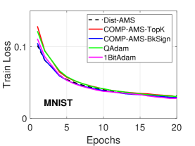
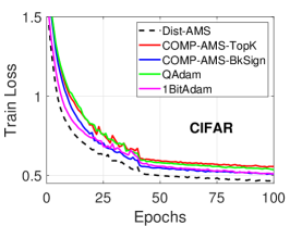
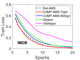
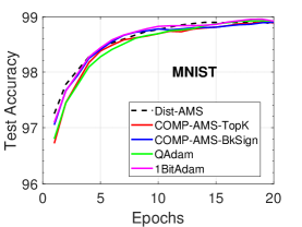
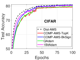
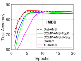
Figure 1: Training loss and test accuracy vs. epochs, on MNIST + CNN, CIFAR-10 + LeNet and IMDB + LSTM with $n=16$ local workers.

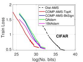
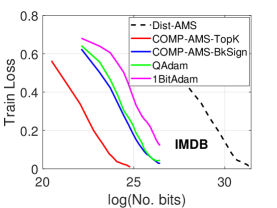
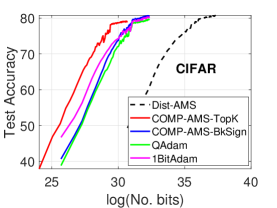
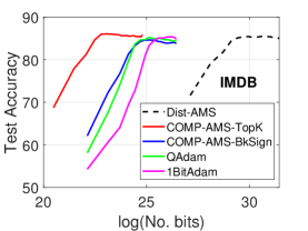
Figure 2: Train loss and Test accuracy vs. No. bits transmitted, on MNIST + CNN, CIFAR-10 + LeNet and IMDB + LSTM with $n=16$ local workers.

5.3 Linear Speedup of Comp-AMS

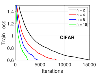
Figure 3: The linear speedup of Comp-AMS with varying $n$. Left: MNIST with Block-Sign compressor on CNN. Right: CIFAR-10 with Top-$k$-0.01 compression on LeNet.

Corollary 2 reveals the linear speedup of Comp-AMS in distributed training. In Figure 3, we present the training loss on MNIST and CIFAR-10 against the number of iterations, with varying number of workers $n$. We use Comp-AMS with Block-Sign on MNIST, and Top-$k$-0.01 on CIFAR. As suggested by the theory, we use $5\times 10^{-4}\sqrt{n}$ as the learning rate. From Figure 3, we see the number of iterations to achieve a certain loss exhibits a strong linear relationship with $n$—it (approximately) decreases by half whenever we double $n$, which justifies the linear speedup of Comp-AMS.

5.4 Discussion

We provide a brief summary of our empirical observations. The proposed Comp-AMS is able to match the learning performance of full-gradient AMSGrad in all the presented experiments. In particular, for data/model involving some sparsity structure, Comp-AMS with the Top-$k$ compressor could be more effective. Also, our results reveal that 1BitAdam might be quite sensitive to the pre-conditioning quality, while Comp-AMS can be more easily tuned and implemented in practice.

We would like to emphasize that, the primary goal of the experiments is to show that Comp-AMS is able to match the performance of full-precision AMSGrad, but not to argue that Comp-AMS is always better than the other algorithms. Since different methods use different underlying optimization algorithms (e.g., AMSGrad, Adam, momentum SGD), comparing Comp-AMS with other distributed training methods would be largely determined by the comparison among these optimization protocols, which is typically data and task dependent. Our results say that: whenever one wants to use AMSGrad to train a deep neural network, she/he can simply employ the distributed Comp-AMS scheme to gain a linear speedup in training time with learning performance as good as the full-precision training, taking little communication cost and memory consumption.

6 Conclusion

In this paper, we study the simple, convenient, yet unexplored gradient averaging strategy for distributed adaptive optimization called Comp-AMS. Top-$k$ and Block-Sign compressor are incorporated for communication efficiency, whose biases are compensated by the error feedback strategy. We develop the convergence rate of Comp-AMS, and show that same as the case of SGD, for AMSGrad, compressed gradient averaging with error feedback matches the convergence of full-gradient AMSGrad, and linear speedup can be obtained in the distributed training. Numerical experiments are conducted to justify the theoretical findings, and demonstrate that Comp-AMS provides comparable performance with other distributed adaptive methods, and achieves similar accuracy as full-precision AMSGrad with significantly reduced communication overhead. Given the simple architecture and hardware (memory) efficiency, we expect Comp-AMS shall be able to serve as a useful and convenient distributed adaptive optimization framework in practice.

Appendix A Tuning Details and More Results on ResNet-18

The search grids of the learning rate of each method can be found in Table 1. Empirically, Dist-AMS, Comp-AMS and 1BitAdam has similar optimal learning rate, while QAdam usually needs larger step size to reach its best performance.

Table 1: Search grids for learning rate tuning.

	Learning rate range
Dist-AMS	$[0.00001,0.00003,0.00005,0.0001,0.0003,0.0005,0.001,0.003,0.005,0.01]$
Comp-AMS	$[0.00001,0.00003,0.00005,0.0001,0.0003,0.0005,0.001,0.003,0.005,0.01]$
QAdam	$[0.0001,0.0003,0.0005,0.001,0.003,0.005,0.01,0.03,0.05,0.1,0.3,0.5]$
1BitAdam	$[0.00001,0.00003,0.00005,0.0001,0.0003,0.0005,0.001,0.003,0.005,0.01]$

We provide more experimental results on CIFAR-10 dataset, trained with ResNet-18 (He et al., 2016). For reference, we also present the result of distributed SGD. As we can see from Figure 4, again Comp-AMS can achieve similar accuracy as AMSGrad, and the Top-$k$ compressor gives the best accuracy, with substantial communication reduction. Note that distributed SGD converges faster than adaptive methods, but the generalization error is slightly worse. This experiment again confirms that Comp-AMS can serve as a simple and convenient distributed adaptive training framework with fast convergence, reduced communication and little performance drop.

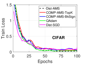
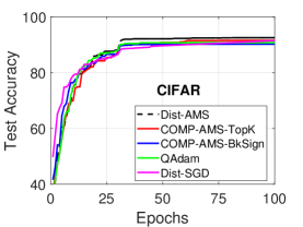
Figure 4: Training loss and test accuracy of different distributed training methods on CIFAR-10 with ResNet-18 (He et al., 2016).

Appendix B Proof of Convergence Results

In this section, we provide the proof of our main result.

B.1 Proof of Theorem 1

Theorem.

Denote $C_{0}=\sqrt{\frac{4(1+q^{2})^{3}}{(1-q^{2})^{2}}G^{2}+\epsilon}$, $C_{1}=\frac{\beta_{1}}{1-\beta_{1}}+\frac{2q}{1-q^{2}}$. Under Assumption 1 to Assumption 4, with $\eta_{t}=\eta\leq\frac{\epsilon}{3C_{0}\sqrt{2L\max\{2L,C_{2}\}}}$, for any $T>0$, Comp-AMS satisfies

$$\frac{1}{T}\sum_{t=1}^{T}\mathbb{E}[\|\nabla f(\theta_{t})\|^{2}] \leq 2C_{0}\Big{(}\frac{\mathbb{E}[f(\theta_{1})-f(\theta^{*})]}{T\eta}+\frac{\eta L\sigma^{2}}{n\epsilon}+\frac{3\eta^{2}LC_{0}C_{1}^{2}\sigma^{2}}{n\epsilon^{2}}$$

$$\hskip 50.58878pt+\frac{12\eta^{2}q^{2}LC_{0}\sigma_{g}^{2}}{(1-q^{2})^{2}\epsilon^{2}}+\frac{(1+C_{1})G^{2}d}{T\sqrt{\epsilon}}+\frac{\eta(1+2C_{1})C_{1}LG^{2}d}{T\epsilon}\Big{)}.$$

Proof.

We first clarify some notations. At time $t$, let the full-precision gradient of the $i$-th worker be $g_{t,i}$, the error accumulator be $e_{t,i}$, and the compressed gradient be $\tilde{g}_{t,i}=\mathcal{C}(g_{t,i}+e_{t,i})$. Slightly different from the notations in the algorithm, we denote $\bar{g}_{t}=\frac{1}{n}\sum_{i=1}^{n}g_{t,i}$, $\overline{\tilde{g}}_{t}=\frac{1}{n}\sum_{i=1}^{n}\tilde{g}_{t,i}$ and $\bar{e}_{t}=\frac{1}{n}\sum_{i=1}^{n}e_{t,i}$. The second moment computed by the compressed gradients is denoted as $v_{t}=\beta_{2}v_{t-1}+(1-\beta_{2})\overline{\tilde{g}}_{t}^{2}$, and $\hat{v}_{t}=\max\{\hat{v}_{t-1},v_{t}\}$. Also, the first order moving average sequence

$$m_{t}=\beta_{1}m_{t-1}+(1-\beta_{1})\overline{\tilde{g}}_{t}\quad \textrm{and}\quad m_{t}^{\prime}=\beta_{1}m_{t-1}^{\prime}+(1-\beta_{1})\bar{g}_{t},$$

where $m_{t}^{\prime}$ represents the first moment moving average sequence using the uncompressed stochastic gradients. By construction we have $m_{t}^{\prime}=(1-\beta_{1})\sum_{\tau=1}^{t}\beta_{1}^{t-\tau}\bar{g}_{\tau}$.

Our proof will use the following auxiliary sequences,

$$\mathcal{E}_{t+1}\mathrel{\mathop{:}}=(1-\beta_{1})\sum_{\tau=1}^{t+1}\beta_{1}^{t+1-\tau}\bar{e}_{\tau},$$

$$\theta_{t+1}^{\prime}:=\theta_{t+1}-\eta\frac{\mathcal{E}_{t+1}}{\sqrt{\hat{v}_{t}+\epsilon}}.$$

Then, we can write the evolution of $\theta_{t}^{\prime}$ as

$$\theta_{t+1}^{\prime} =\theta_{t+1}-\eta\frac{\mathcal{E}_{t+1}}{\sqrt{\hat{v}_{t}+\epsilon}}$$

$$=\theta_{t}-\eta\frac{(1-\beta_{1})\sum_{\tau=1}^{t}\beta_{1}^{t-\tau}\overline{\tilde{g}}_{\tau}+(1-\beta_{1})\sum_{\tau=1}^{t+1}\beta_{1}^{t+1-\tau}\bar{e}_{\tau}}{\sqrt{\hat{v}_{t}+\epsilon}}$$

$$=\theta_{t}-\eta\frac{(1-\beta_{1})\sum_{\tau=1}^{t}\beta_{1}^{t-\tau}(\overline{\tilde{g}}_{\tau}+\bar{e}_{\tau+1})+(1-\beta)\beta_{1}^{t}\bar{e}_{1}}{\sqrt{\hat{v}_{t}+\epsilon}}$$

$$=\theta_{t}-\eta\frac{(1-\beta_{1})\sum_{\tau=1}^{t}\beta_{1}^{t-\tau}\bar{e}_{\tau}}{\sqrt{\hat{v}_{t}+\epsilon}}-\eta\frac{m_{t}^{\prime}}{\sqrt{\hat{v}_{t}+\epsilon}}$$

$$=\theta_{t}-\eta\frac{\mathcal{E}_{t}}{\sqrt{\hat{v}_{t-1}+\epsilon}}-\eta\frac{m_{t}^{\prime}}{\sqrt{\hat{v}_{t}+\epsilon}}+\eta(\frac{1}{\sqrt{\hat{v}_{t-1}+\epsilon}}-\frac{1}{\sqrt{\hat{v}_{t}+\epsilon}})\mathcal{E}_{t}$$

$$\overset{(a)}{=}\theta_{t}^{\prime}-\eta\frac{m_{t}^{\prime}}{\sqrt{\hat{v}_{t}+\epsilon}}+\eta(\frac{1}{\sqrt{\hat{v}_{t-1}+\epsilon}}-\frac{1}{\sqrt{\hat{v}_{t}+\epsilon}})\mathcal{E}_{t}$$

$$\mathrel{\mathop{:}}=\theta_{t}^{\prime}-\eta\frac{m_{t}^{\prime}}{\sqrt{\hat{v}_{t}+\epsilon}}+\eta D_{t}\mathcal{E}_{t},$$

where (a) uses the fact that for every $i\in[n]$, $\tilde{g}_{t,i}+e_{{t+1,i}}=g_{t,i}+e_{t,i}$, and $e_{t,1}=0$ at initialization. Further define the virtual iterates:

$$x_{t+1}\mathrel{\mathop{:}}=\theta_{t+1}^{\prime}-\eta\frac{\beta_{1}}{1-\beta_{1}}\frac{m_{t}^{\prime}}{\sqrt{\hat{v}_{t}+\epsilon}},$$

which follows the recurrence:

$$x_{t+1} =\theta_{t+1}^{\prime}-\eta\frac{\beta_{1}}{1-\beta_{1}}\frac{m_{t}^{\prime}}{\sqrt{\hat{v}_{t}+\epsilon}}$$

$$=\theta_{t}^{\prime}-\eta\frac{m_{t}^{\prime}}{\sqrt{\hat{v}_{t}+\epsilon}}-\eta\frac{\beta_{1}}{1-\beta_{1}}\frac{m_{t}^{\prime}}{\sqrt{\hat{v}_{t}+\epsilon}}+\eta D_{t}\mathcal{E}_{t}$$

$$=\theta_{t}^{\prime}-\eta\frac{\beta_{1}m_{t-1}^{\prime}+(1-\beta_{1})\bar{g}_{t}+\frac{\beta_{1}^{2}}{1-\beta_{1}}m_{t-1}^{\prime}+\beta_{1}\bar{g}_{t}}{\sqrt{\hat{v}_{t}+\epsilon}}+\eta D_{t}\mathcal{E}_{t}$$

$$=\theta_{t}^{\prime}-\eta\frac{\beta_{1}}{1-\beta_{1}}\frac{m_{t-1}^{\prime}}{\sqrt{\hat{v}_{t}+\epsilon}}-\eta\frac{\bar{g}_{t}}{\sqrt{\hat{v}_{t}+\epsilon}}+\eta D_{t}\mathcal{E}_{t}$$

$$=x_{t}-\eta\frac{\bar{g}_{t}}{\sqrt{\hat{v}_{t}+\epsilon}}+\eta\frac{\beta_{1}}{1-\beta_{1}}D_{t}m_{t-1}^{\prime}+\eta D_{t}\mathcal{E}_{t}.$$

When summing over $t=1,...,T$, the difference sequence $D_{t}$ satisfies the bounds of Lemma 5.

By the smoothness Assumption 2, we have

$$f(x_{t+1})\leq f(x_{t})+\langle\nabla f(x_{t}),x_{t+1}-x_{t}\rangle+\frac{L}{2}\|x_{t+1}-x_{t}\|^{2}.$$

Taking expectation w.r.t. the randomness at time $t$, we obtain

$$\mathbb{E}[f(x_{t+1})]-f(x_{t})$$

$$\leq-\eta\mathbb{E}[\langle\nabla f(x_{t}),\frac{\bar{g}_{t}}{\sqrt{\hat{v}_{t}+\epsilon}}\rangle]+\eta\mathbb{E}[\langle\nabla f(x_{t}),\frac{\beta_{1}}{1-\beta_{1}}D_{t}m_{t-1}^{\prime}+D_{t}\mathcal{E}_{t}\rangle]$$

$$\hskip 144.54pt+\frac{\eta^{2}L}{2}\mathbb{E}[\|\frac{\bar{g}_{t}}{\sqrt{\hat{v}_{t}+\epsilon}}-\frac{\beta_{1}}{1-\beta_{1}}D_{t}m_{t-1}^{\prime}-D_{t}\mathcal{E}_{t}\|^{2}]$$

$$=\underbrace{-\eta\mathbb{E}[\langle\nabla f(\theta_{t}),\frac{\bar{g}_{t}}{\sqrt{\hat{v}_{t}+\epsilon}}\rangle]}_{I}+\underbrace{\eta\mathbb{E}[\langle\nabla f(x_{t}),\frac{\beta_{1}}{1-\beta_{1}}D_{t}m_{t-1}^{\prime}+D_{t}\mathcal{E}_{t}\rangle]}_{II}$$

$$\hskip 36.135pt+\underbrace{\frac{\eta^{2}L}{2}\mathbb{E}[\|\frac{\bar{g}_{t}}{\sqrt{\hat{v}_{t}+\epsilon}}-\frac{\beta_{1}}{1-\beta_{1}}D_{t}m_{t-1}^{\prime}-D_{t}\mathcal{E}_{t}\|^{2}]}_{III}+\underbrace{\eta\mathbb{E}[\langle\nabla f(\theta_{t})-\nabla f(x_{t}),\frac{\bar{g}_{t}}{\sqrt{\hat{v}_{t}+\epsilon}}\rangle]}_{IV},$$ (3)

In the following, we bound the terms separately.

Bounding term I. We have

$$I =-\eta\mathbb{E}[\langle\nabla f(\theta_{t}),\frac{\bar{g}_{t}}{\sqrt{\hat{v}_{t-1}+\epsilon}}]-\eta\mathbb{E}[\langle\nabla f(\theta_{t}),(\frac{1}{\sqrt{\hat{v}_{t}+\epsilon}}-\frac{1}{\sqrt{\hat{v}_{t-1}+\epsilon}})\bar{g}_{t}\rangle]$$

$$\leq-\eta\mathbb{E}[\langle\nabla f(\theta_{t}),\frac{\nabla f(\theta_{t})}{\sqrt{\hat{v}_{t-1}+\epsilon}}]+\eta G^{2}\mathbb{E}[\|D_{t}\|].$$

$$\leq-\frac{\eta}{\sqrt{\frac{4(1+q^{2})^{3}}{(1-q^{2})^{2}}G^{2}+\epsilon}}\mathbb{E}[\|\nabla f(\theta_{t})\|^{2}]+\eta G^{2}\mathbb{E}[\|D_{t}\|_{1}],$$ (4)

where we use Assumption 3, Lemma 4 and the fact that $l_{2}$ norm is no larger than $l_{1}$ norm.

Bounding term II. By the definition of $\mathcal{E}_{t}$, we know that $\|\mathcal{E}_{t}\|\leq(1-\beta_{1})\sum_{\tau=1}^{t}\beta_{1}^{t-\tau}\|\bar{e}_{t}\|\leq\frac{2q}{1-q^{2}}G$. Then we have

$$II \leq\eta(\mathbb{E}[\langle\nabla f(\theta_{t}),\frac{\beta_{1}}{1-\beta_{1}}D_{t}m_{t-1}^{\prime}+D_{t}\mathcal{E}_{t}\rangle]+\mathbb{E}[\langle\nabla f(x_{t})-\nabla f(\theta_{t}),\frac{\beta_{1}}{1-\beta_{1}}D_{t}m_{t-1}^{\prime}+D_{t}\mathcal{E}_{t}\rangle])$$

$$\leq\eta\mathbb{E}[\|\nabla f(\theta_{t})\|\|\frac{\beta_{1}}{1-\beta_{1}}D_{t}m_{t-1}^{\prime}+D_{t}\mathcal{E}_{t}\|]+\eta^{2}\ L\mathbb{E}[\|\frac{\frac{\beta_{1}}{1-\beta_{1}}m_{t-1}^{\prime}+\mathcal{E}_{t}}{\sqrt{\hat{v}_{t-1}+\epsilon}}\|\|\frac{\beta_{1}}{1-\beta_{1}}D_{t}m_{t-1}^{\prime}+D_{t}\mathcal{E}_{t}\|]$$

$$\leq\eta C_{1}G^{2}\mathbb{E}[\|D_{t}\|_{1}]+\frac{\eta^{2}C_{1}^{2}LG^{2}}{\sqrt{\epsilon}}\mathbb{E}[\|D_{t}\|_{1}],$$ (5)

where $C_{1}\mathrel{\mathop{:}}=\frac{\beta_{1}}{1-\beta_{1}}+\frac{2q}{1-q^{2}}$. The second inequality is because of smoothness of $f(\theta)$, and the last inequality is due to Lemma 2, Assumption 3 and the property of norms.

Bounding term III. This term can be bounded as follows:

$$III \leq\eta^{2}L\mathbb{E}[\|\frac{\bar{g}_{t}}{\sqrt{\hat{v}_{t}+\epsilon}}\|^{2}]+\eta^{2}L\mathbb{E}[\|\frac{\beta_{1}}{1-\beta_{1}}D_{t}m_{t-1}^{\prime}-D_{t}\mathcal{E}_{t}\|^{2}]]$$

$$\leq\frac{\eta^{2}L}{\epsilon}\mathbb{E}[\|\frac{1}{n}\sum_{i=1}^{n}g_{t,i}-\nabla f(\theta_{t})+\nabla f(\theta_{t})\|^{2}]+\eta^{2}L\mathbb{E}[\|D_{t}(\frac{\beta_{1}}{1-\beta_{1}}m_{t-1}^{\prime}-\mathcal{E}_{t})\|^{2}]$$

$$\overset{(a)}{\leq}\frac{\eta^{2}L}{\epsilon}\mathbb{E}[\|\nabla f(\theta_{t})\|^{2}]+\frac{\eta^{2}L\sigma^{2}}{n\epsilon}+\eta^{2}C_{1}^{2}LG^{2}\mathbb{E}[\|D_{t}\|^{2}],$$ (6)

where (a) follows from $\nabla f(\theta_{t})=\frac{1}{n}\sum_{i=1}^{n}\nabla f_{i}(\theta_{t})$ and Assumption 4 that $g_{t,i}$ is unbiased of $\nabla f_{i}(\theta_{t})$ and has bounded variance $\sigma^{2}$.

Bounding term IV. We have

$$IV =\eta\mathbb{E}[\langle\nabla f(\theta_{t})-\nabla f(x_{t}),\frac{\bar{g}_{t}}{\sqrt{\hat{v}_{t-1}+\epsilon}}\rangle]+\eta\mathbb{E}[\langle\nabla f(\theta_{t})-\nabla f(x_{t}),(\frac{1}{\sqrt{\hat{v}_{t}+\epsilon}}-\frac{1}{\sqrt{\hat{v}_{t-1}+\epsilon}})\bar{g}_{t}\rangle]$$

$$\leq\eta\mathbb{E}[\langle\nabla f(\theta_{t})-\nabla f(x_{t}),\frac{\nabla f(\theta_{t})}{\sqrt{\hat{v}_{t-1}+\epsilon}}\rangle]+\eta^{2}L\mathbb{E}[\|\frac{\frac{\beta_{1}}{1-\beta_{1}}m_{t-1}^{\prime}+\mathcal{E}_{t}}{\sqrt{\hat{v}_{t-1}+\epsilon}}\|\|D_{t}g_{t}\|]$$

$$\overset{(a)}{\leq}\frac{\eta\rho}{2\epsilon}\mathbb{E}[\|\nabla f(\theta_{t})\|^{2}]+\frac{\eta}{2\rho}\mathbb{E}[\|\nabla f(\theta_{t})-\nabla f(x_{t})\|^{2}]+\frac{\eta^{2}C_{1}LG^{2}}{\sqrt{\epsilon}}\mathbb{E}[\|D_{t}\|]$$

$$\overset{(b)}{\leq}\frac{\eta\rho}{2\epsilon}\mathbb{E}[\|\nabla f(\theta_{t})\|^{2}]+\frac{\eta^{3}L}{2\rho}\mathbb{E}[\|\frac{\frac{\beta_{1}}{1-\beta_{1}}m_{t-1}^{\prime}+\mathcal{E}_{t}}{\sqrt{\hat{v}_{t-1}+\epsilon}}\|^{2}]+\frac{\eta^{2}C_{1}LG^{2}}{\sqrt{\epsilon}}\mathbb{E}[\|D_{t}\|_{1}],$$ (7)

where (a) is due to Young’s inequality and (b) is based on Assumption 2.

Regarding the second term in (7), by Lemma 3 and Lemma 1, summing over $t=1,...,T$ we have

$$\sum_{t=1}^{T}\frac{\eta^{3}L}{2\rho}\mathbb{E}[\|\frac{\frac{\beta_{1}}{1-\beta_{1}}m_{t-1}^{\prime}+\mathcal{E}_{t}}{\sqrt{\hat{v}_{t-1}+\epsilon}}\|^{2}]$$

$$\leq\sum_{t=1}^{T}\frac{\eta^{3}L}{2\rho\epsilon}\mathbb{E}[\|\frac{\beta_{1}}{1-\beta_{1}}m_{t-1}^{\prime}+\mathcal{E}_{t}\|^{2}]$$

$$\leq\sum_{t=1}^{T}\frac{\eta^{3}L}{\rho\epsilon}\Big{[}\frac{\beta_{1}^{2}}{(1-\beta_{1})^{2}}\mathbb{E}[\|m_{t}^{\prime}\|^{2}]+\mathbb{E}[\|\mathcal{E}_{t}\|^{2}]\Big{]}$$

$$\leq\frac{T\eta^{3}\beta_{1}^{2}L\sigma^{2}}{n\rho(1-\beta_{1})^{2}\epsilon}+\frac{\eta^{3}\beta_{1}^{2}L}{\rho(1-\beta_{1})^{2}\epsilon}\sum_{t=1}^{T}\mathbb{E}[\|\nabla f(\theta_{t})\|^{2}]$$

$$\hskip 144.54pt+\frac{4T\eta^{3}q^{2}L}{\rho(1-q^{2})^{2}\epsilon}(\sigma^{2}+\sigma_{g}^{2})+\frac{4\eta^{3}q^{2}L}{\rho(1-q^{2})^{2}\epsilon}\sum_{t=1}^{T}\mathbb{E}[\|\nabla f(\theta_{t})\|^{2}]$$

$$=\frac{T\eta^{3}LC_{2}\sigma^{2}}{n\rho\epsilon}+\frac{4T\eta^{3}q^{2}L\sigma_{g}^{2}}{\rho(1-q^{2})^{2}\epsilon}+\frac{\eta^{3}LC_{2}}{\rho\epsilon}\sum_{t=1}^{T}\mathbb{E}[\|\nabla f(\theta_{t})\|^{2}],$$ (8)

with $C_{2}\mathrel{\mathop{:}}=\frac{\beta_{1}^{2}}{(1-\beta_{1})^{2}}+\frac{4q^{2}}{(1-q^{2})^{2}}$. Now integrating (4), (5), (6), (7) and (8) into (3), taking the telescoping summation over $t=1,...,T$, we obtain

$$\mathbb{E}[f(x_{T+1})-f(x_{1})]$$

$$\leq(-\frac{\eta}{C_{0}}+\frac{\eta^{2}L}{\epsilon}+\frac{\eta\rho}{2\epsilon}+\frac{\eta^{3}LC_{2}}{\rho\epsilon})\sum_{t=1}^{T}\mathbb{E}[\|\nabla f(\theta_{t})\|^{2}]+\frac{T\eta^{2}L\sigma^{2}}{n\epsilon}+\frac{T\eta^{3}LC_{2}\sigma^{2}}{n\rho\epsilon}+\frac{4T\eta^{3}q^{2}L\sigma_{g}^{2}}{\rho(1-q^{2})^{2}\epsilon}$$

$$\hskip 57.81621pt+(\eta(1+C_{1})G^{2}+\frac{\eta^{2}(1+C_{1})C_{1}LG^{2}}{\sqrt{\epsilon}})\sum_{t=1}^{T}\mathbb{E}[\|D_{t}\|_{1}]+\eta^{2}C_{1}^{2}LG^{2}\sum_{t=1}^{T}\mathbb{E}[\|D_{t}\|^{2}.$$

with $C_{0}\mathrel{\mathop{:}}=\sqrt{\frac{4(1+q^{2})^{3}}{(1-q^{2})^{2}}G^{2}+\epsilon}$. Setting $\eta\leq\frac{\epsilon}{3C_{0}\sqrt{2L\max\{2L,C_{2}\}}}$ and choosing $\rho=\frac{\epsilon}{3C_{0}}$, we further arrive at

$$\mathbb{E}[f(x_{T+1})-f(x_{1})]$$

$$\leq-\frac{\eta}{2C_{0}}\sum_{t=1}^{T}\mathbb{E}[\|\nabla f(\theta_{t})\|^{2}]+\frac{T\eta^{2}L\sigma^{2}}{n\epsilon}+\frac{3T\eta^{3}LC_{0}C_{2}\sigma^{2}}{n\epsilon^{2}}+\frac{12T\eta^{3}q^{2}LC_{0}\sigma_{g}^{2}}{(1-q^{2})^{2}\epsilon^{2}}$$

$$\hskip 158.99377pt+\frac{\eta(1+C_{1})G^{2}d}{\sqrt{\epsilon}}+\frac{\eta^{2}(1+2C_{1})C_{1}LG^{2}d}{\epsilon}.$$

where the inequality follows from Lemma 5. Re-arranging terms, we get that

$$\frac{1}{T}\sum_{t=1}^{T}\mathbb{E}[\|\nabla f(\theta_{t})\|^{2}] \leq 2C_{0}\Big{(}\frac{\mathbb{E}[f(x_{1})-f(x_{T+1})]}{T\eta}+\frac{\eta L\sigma^{2}}{n\epsilon}+\frac{3\eta^{2}LC_{0}C_{2}\sigma^{2}}{n\epsilon^{2}}$$

$$\hskip 50.58878pt+\frac{12\eta^{2}q^{2}LC_{0}\sigma_{g}^{2}}{(1-q^{2})^{2}\epsilon^{2}}+\frac{(1+C_{1})G^{2}d}{T\sqrt{\epsilon}}+\frac{\eta(1+2C_{1})C_{1}LG^{2}d}{T\epsilon}\Big{)}$$

$$\leq 2C_{0}\Big{(}\frac{\mathbb{E}[f(\theta_{1})-f(\theta^{*})]}{T\eta}+\frac{\eta L\sigma^{2}}{n\epsilon}+\frac{3\eta^{2}LC_{0}C_{1}^{2}\sigma^{2}}{n\epsilon^{2}}$$

$$\hskip 50.58878pt+\frac{12\eta^{2}q^{2}LC_{0}\sigma_{g}^{2}}{(1-q^{2})^{2}\epsilon^{2}}+\frac{(1+C_{1})G^{2}d}{T\sqrt{\epsilon}}+\frac{\eta(1+2C_{1})C_{1}LG^{2}d}{T\epsilon}\Big{)},$$

where $C_{0}=\sqrt{\frac{4(1+q^{2})^{3}}{(1-q^{2})^{2}}G^{2}+\epsilon}$, $C_{1}=\frac{\beta_{1}}{1-\beta_{1}}+\frac{2q}{1-q^{2}}$. The last inequality is because $x_{1}=\theta_{1}$, $\theta^{*}\mathrel{\mathop{:}}=\operatorname*{arg\,min}_{\theta}f(\theta)$ and the fact that $C_{2}\leq C_{1}^{2}$. This completes the proof. ∎

B.2 Intermediate Lemmata

The lemmas used in the proof of Theorem 1 are given as below.

Lemma 1.

Under Assumption 1 to Assumption 4 we have:

$$\|m_{t}^{\prime}\|\leq G,\quad\forall t,$$

$$\sum_{t=1}^{T}\mathbb{E}\|m_{t}^{\prime}\|^{2}\leq\frac{T\sigma^{2}}{n}+\sum_{t=1}^{T}\mathbb{E}[\|\nabla f(\theta_{t})\|^{2}].$$

Proof.

For the first part, it is easy to see that by Assumption 3,

$$\|m_{t}^{\prime}\| =(1-\beta_{1})\|\sum_{\tau=1}^{t}\beta_{1}^{t-\tau}\bar{g}_{t}\|\leq G.$$

For the second claim, the expected squared norm of average stochastic gradient can be bounded by

$$\mathbb{E}[\|\bar{g}_{t}^{2}\|] =\mathbb{E}[\|\frac{1}{n}\sum_{i=1}^{n}g_{t,i}-\nabla f(\theta_{t})+\nabla f(\theta_{t})\|^{2}]$$

$$=\mathbb{E}[\|\frac{1}{n}\sum_{i=1}^{n}(g_{t,i}-\nabla f_{i}(\theta_{t}))\|^{2}]+\mathbb{E}[\|\nabla f(\theta_{t})\|^{2}]$$

$$\leq\frac{\sigma^{2}}{n}+\mathbb{E}[\|\nabla f(\theta_{t})\|^{2}],$$

where we use Assumption 4 that $g_{t,i}$ is unbiased with bounded variance. Let $\bar{g}_{t,j}$ denote the $j$-th coordinate of $\bar{g}_{t}$. By the updating rule of Comp-AMS, we have

$$\mathbb{E}[\|m_{t}^{\prime}\|^{2}] =\mathbb{E}[\|(1-\beta_{1})\sum_{\tau=1}^{t}\beta_{1}^{t-\tau}\bar{g}_{\tau}\|^{2}]$$

$$\leq(1-\beta_{1})^{2}\sum_{j=1}^{d}\mathbb{E}[(\sum_{\tau=1}^{t}\beta_{1}^{t-\tau}\bar{g}_{\tau,j})^{2}]$$

$$\overset{(a)}{\leq}(1-\beta_{1})^{2}\sum_{j=1}^{d}\mathbb{E}[(\sum_{\tau=1}^{t}\beta_{1}^{t-\tau})(\sum_{\tau=1}^{t}\beta_{1}^{t-\tau}\bar{g}_{\tau,j}^{2})]$$

$$\leq(1-\beta_{1})\sum_{\tau=1}^{t}\beta_{1}^{t-\tau}\mathbb{E}[\|\bar{g}_{\tau}\|^{2}]$$

$$\leq\frac{\sigma^{2}}{n}+(1-\beta_{1})\sum_{\tau=1}^{t}\beta_{1}^{t-\tau}\mathbb{E}[\|\nabla f(\theta_{t})\|^{2}],$$

where (a) is due to Cauchy-Schwartz inequality. Summing over $t=1,...,T$, we obtain

$$\sum_{t=1}^{T}\mathbb{E}\|m_{t}^{\prime}\|^{2}\leq\frac{T\sigma^{2}}{n}+\sum_{t=1}^{T}\mathbb{E}[\|\nabla f(\theta_{t})\|^{2}].$$

This completes the proof. ∎

Lemma 2.

Under Assumption 4, we have for $\forall t$ and each local worker $\forall i\in[n]$,

$$\|e_{t,i}\|^{2}\leq\frac{4q^{2}}{(1-q^{2})^{2}}G^{2},$$

$$\mathbb{E}[\|e_{t+1,i}\|^{2}]\leq\frac{4q^{2}}{(1-q^{2})^{2}}\sigma^{2}+\frac{2q^{2}}{1-q^{2}}\sum_{\tau=1}^{t}(\frac{1+q^{2}}{2})^{t-\tau}\mathbb{E}[\|\nabla f_{i}(\theta_{\tau})\|^{2}].$$

Proof.

We start by using Assumption 1 and Young’s inequality to get

$$\|e_{t+1,i}\|^{2} =\|g_{t,i}+e_{t,i}-\mathcal{C}(g_{t,i}+e_{t,i})\|^{2}$$

$$\leq q^{2}\|g_{t,i}+e_{t,i}\|^{2}$$

$$\leq q^{2}(1+\rho)\|e_{t,i}\|^{2}+q^{2}(1+\frac{1}{\rho})\|g_{t,i}\|^{2}$$

$$\leq\frac{1+q^{2}}{2}\|e_{t,i}\|^{2}+\frac{2q^{2}}{1-q^{2}}\|g_{t,i}\|^{2},$$ (9)

where (9) is derived by choosing $\rho=\frac{1-q^{2}}{2q^{2}}$ and the fact that $q<1$. Now by recursion and the initialization $e_{1,i}=0$, we have

$$\mathbb{E}[\|e_{t+1,i}\|^{2}] \leq\frac{2q^{2}}{1-q^{2}}\sum_{\tau=1}^{t}(\frac{1+q^{2}}{2})^{t-\tau}\mathbb{E}[\|g_{\tau,i}\|^{2}]$$

$$\leq\frac{4q^{2}}{(1-q^{2})^{2}}\sigma^{2}+\frac{2q^{2}}{1-q^{2}}\sum_{\tau=1}^{t}(\frac{1+q^{2}}{2})^{t-\tau}\mathbb{E}[\|\nabla f_{i}(\theta_{\tau})\|^{2}],$$

which proves the second argument. Meanwhile, the absolute bound $\|e_{t,i}\|^{2}\leq\frac{4q^{2}}{(1-q^{2})^{2}}G^{2}$ follows directly from (9). ∎

Lemma 3.

For the moving average error sequence $\mathcal{E}_{t}$, it holds that

$$\sum_{t=1}^{T}\mathbb{E}[\|\mathcal{E}_{t}\|^{2}]\leq\frac{4Tq^{2}}{(1-q^{2})^{2}}(\sigma^{2}+\sigma_{g}^{2})+\frac{4q^{2}}{(1-q^{2})^{2}}\sum_{t=1}^{T}\mathbb{E}[\|\nabla f(\theta_{t})\|^{2}].$$

Proof.

Denote $K_{t,i}\mathrel{\mathop{:}}=\sum_{\tau=1}^{t}(\frac{1+q^{2}}{2})^{t-\tau}\mathbb{E}[\|\nabla f_{i}(\theta_{\tau})\|^{2}]$. Using the same technique as in the proof of Lemma 1, denoting $\bar{e}_{t,j}$ as the $j$-th coordinate of $\bar{e}_{t}$, it follows that

$$\mathbb{E}[\|\mathcal{E}_{t}\|^{2}] =\mathbb{E}[\|(1-\beta_{1})\sum_{\tau=1}^{t}\beta_{1}^{t-\tau}\bar{e}_{\tau}\|^{2}]$$

$$\leq(1-\beta_{1})^{2}\sum_{j=1}^{d}\mathbb{E}[(\sum_{\tau=1}^{t}\beta_{1}^{t-\tau}\bar{e}_{\tau,j})^{2}]$$

$$\overset{(a)}{\leq}(1-\beta_{1})^{2}\sum_{j=1}^{d}\mathbb{E}[(\sum_{\tau=1}^{t}\beta_{1}^{t-\tau})(\sum_{\tau=1}^{t}\beta_{1}^{t-\tau}\bar{e}_{\tau,j}^{2})]$$

$$\leq(1-\beta_{1})\sum_{\tau=1}^{t}\beta_{1}^{t-\tau}\mathbb{E}[\|\bar{e}_{\tau}\|^{2}]$$

$$\leq(1-\beta_{1})\sum_{\tau=1}^{t}\beta_{1}^{t-\tau}\mathbb{E}[\frac{1}{n}\sum_{i=1}^{n}\|e_{\tau,i}\|^{2}]$$

$$\overset{(b)}{\leq}\frac{4q^{2}}{(1-q^{2})^{2}}\sigma^{2}+\frac{2q^{2}(1-\beta_{1})}{(1-q^{2})}\sum_{\tau=1}^{t}\beta_{1}^{t-\tau}(\frac{1}{n}\sum_{i=1}^{n}K_{\tau,i}),$$

where (a) is due to Cauchy-Schwartz and (b) is a result of Lemma 2. Summing over $t=1,...,T$ and using the technique of geometric series summation leads to

$$\sum_{t=1}^{T}\mathbb{E}[\|\mathcal{E}_{t}\|^{2}] \leq\frac{4Tq^{2}}{(1-q^{2})^{2}}\sigma^{2}+\frac{2q^{2}(1-\beta_{1})}{(1-q^{2})}\sum_{t=1}^{T}\sum_{\tau=1}^{t}\beta_{1}^{t-\tau}(\frac{1}{n}\sum_{i=1}^{n}K_{\tau,i})$$

$$\leq\frac{4Tq^{2}}{(1-q^{2})^{2}}\sigma^{2}+\frac{2q^{2}}{(1-q^{2})}\sum_{t=1}^{T}\sum_{\tau=1}^{t}(\frac{1+q^{2}}{2})^{t-\tau}\mathbb{E}[\frac{1}{n}\sum_{i=1}^{n}\|\nabla f_{i}(\theta_{\tau})\|^{2}]$$

$$\leq\frac{4Tq^{2}}{(1-q^{2})^{2}}\sigma^{2}+\frac{4q^{2}}{(1-q^{2})^{2}}\sum_{t=1}^{T}\mathbb{E}[\frac{1}{n}\sum_{i=1}^{n}\|\nabla f_{i}(\theta_{t})\|^{2}]$$

$$\overset{(a)}{\leq}\frac{4Tq^{2}}{(1-q^{2})^{2}}\sigma^{2}+\frac{4q^{2}}{(1-q^{2})^{2}}\sum_{t=1}^{T}\mathbb{E}[\|\frac{1}{n}\sum_{i=1}^{n}\nabla f_{i}(\theta_{t})\|^{2}+\frac{1}{n}\sum_{i=1}^{n}\|\nabla f_{i}(\theta_{t})-\nabla f(\theta_{t})\|^{2}]$$

$$\leq\frac{4Tq^{2}}{(1-q^{2})^{2}}(\sigma^{2}+\sigma_{g}^{2})+\frac{4q^{2}}{(1-q^{2})^{2}}\sum_{t=1}^{T}\mathbb{E}[\|\nabla f(\theta_{t})\|^{2}],$$

where (a) is derived by the variance decomposition and the last inequality holds due to Assumption 4. The desired result is obtained. ∎

Lemma 4.

It holds that $\forall t\in[T]$, $\forall i\in[d]$, $\hat{v}_{t,i}\leq\frac{4(1+q^{2})^{3}}{(1-q^{2})^{2}}G^{2}$.

Proof.

For any $t$, by Lemma 2 and Assumption 3 we have

$$\|\tilde{g}_{t}\|^{2} =\|\mathcal{C}(g_{t}+e_{t})\|^{2}$$

$$\leq\|\mathcal{C}(g_{t}+e_{t})-(g_{t}+e_{t})+(g_{t}+e_{t})\|^{2}$$

$$\leq 2(q^{2}+1)\|g_{t}+e_{t}\|^{2}$$

$$\leq 4(q^{2}+1)(G^{2}+\frac{4q^{2}}{(1-q^{2})^{2}}G^{2})$$

$$=\frac{4(1+q^{2})^{3}}{(1-q^{2})^{2}}G^{2}.$$

It’s then easy to show by the updating rule of $\hat{v}_{t}$, there exists a $j\in[t]$ such that $\hat{v}_{t}=v_{j}$. Then

$$\hat{v}_{t,i}=(1-\beta_{2})\sum_{\tau=1}^{j}\beta_{2}^{j-\tau}\tilde{g}_{\tau,i}^{2}\leq\frac{4(1+q^{2})^{3}}{(1-q^{2})^{2}}G^{2},$$

which concludes the claim. ∎

Lemma 5.

Let $D_{t}\mathrel{\mathop{:}}=\frac{1}{\sqrt{\hat{v}_{t-1}+\epsilon}}-\frac{1}{\sqrt{\hat{v}_{t}+\epsilon}}$ be defined as above. Then,

$$\sum_{t=1}^{T}\|D_{t}\|_{1}\leq\frac{d}{\sqrt{\epsilon}},\quad\sum_{t=1}^{T}\|D_{t}\|^{2}\leq\frac{d}{\epsilon}.$$

Proof.

By the updating rule of Comp-AMS, $\hat{v}_{t-1}\leq\hat{v}_{t}$ for $\forall t$. Therefore, by the initialization $\hat{v}_{0}=0$, we have

$$\sum_{t=1}^{T}\|D_{t}\|_{1} =\sum_{t=1}^{T}\sum_{i=1}^{d}(\frac{1}{\sqrt{\hat{v}_{t-1,i}+\epsilon}}-\frac{1}{\sqrt{\hat{v}_{t,i}+\epsilon}})$$

$$=\sum_{i=1}^{d}(\frac{1}{\sqrt{\hat{v}_{0,i}+\epsilon}}-\frac{1}{\sqrt{\hat{v}_{T,i}+\epsilon}})$$

$$\leq\frac{d}{\sqrt{\epsilon}}.$$

For the sum of squared $l_{2}$ norm, note the fact that for $a\geq b>0$, it holds that

$$(a-b)^{2}\leq(a-b)(a+b)=a^{2}-b^{2}.$$

Thus,

$$\sum_{t=1}^{T}\|D_{t}\|^{2} =\sum_{t=1}^{T}\sum_{i=1}^{d}(\frac{1}{\sqrt{\hat{v}_{t-1,i}+\epsilon}}-\frac{1}{\sqrt{\hat{v}_{t,i}+\epsilon}})^{2}$$

$$\leq\sum_{t=1}^{T}\sum_{i=1}^{d}(\frac{1}{\hat{v}_{t-1,i}+\epsilon}-\frac{1}{\hat{v}_{t,i}+\epsilon})$$

$$\leq\frac{d}{\epsilon},$$

which gives the desired result. ∎

References

- Agarwal et al. (2018) Naman Agarwal, Ananda Theertha Suresh, Felix X. Yu, Sanjiv Kumar, and Brendan McMahan. cpSGD: Communication-efficient and differentially-private distributed SGD. In Advances in Neural Information Processing Systems (NeurIPS), pp. 7575–7586, Montréal, Canada, 2018.
- Ajalloeian & Stich (2020) Ahmad Ajalloeian and Sebastian U Stich. Analysis of SGD with biased gradient estimators. arXiv preprint arXiv:2008.00051, 2020.
- Aji & Heafield (2017) Alham Fikri Aji and Kenneth Heafield. Sparse communication for distributed gradient descent. In Proceedings of the 2017 Conference on Empirical Methods in Natural Language Processing (EMNLP), pp. 440–445, Copenhagen, Denmark, 2017.
- Alistarh et al. (2017) Dan Alistarh, Demjan Grubic, Jerry Li, Ryota Tomioka, and Milan Vojnovic. QSGD: communication-efficient SGD via gradient quantization and encoding. In Advances in Neural Information Processing Systems (NIPS), pp. 1709–1720, Long Beach, CA, 2017.
- Alistarh et al. (2018) Dan Alistarh, Torsten Hoefler, Mikael Johansson, Nikola Konstantinov, Sarit Khirirat, and Cédric Renggli. The convergence of sparsified gradient methods. In Advances in Neural Information Processing Systems (NeurIPS), pp. 5977–5987, Montréal, Canada, 2018.
- Basu et al. (2019) Debraj Basu, Deepesh Data, Can Karakus, and Suhas N. Diggavi. Qsparse-local-sgd: Distributed SGD with quantization, sparsification and local computations. In Advances in Neural Information Processing Systems (NeurIPS), pp. 14668–14679, Vancouver, Canada, 2019.
- Bernstein et al. (2018) Jeremy Bernstein, Yu-Xiang Wang, Kamyar Azizzadenesheli, and Animashree Anandkumar. SIGNSGD: compressed optimisation for non-convex problems. In Proceedings of the 35th International Conference on Machine Learning (ICML), pp. 559–568, Stockholmsmässan, Stockholm, Sweden, 2018.
- Bernstein et al. (2019) Jeremy Bernstein, Jiawei Zhao, Kamyar Azizzadenesheli, and Anima Anandkumar. signSGD with majority vote is communication efficient and fault tolerant. In Proceedings of the 7th International Conference on Learning Representations (ICLR), New Orleans, LA, 2019.
- Beznosikov et al. (2020) Aleksandr Beznosikov, Samuel Horváth, Peter Richtárik, and Mher Safaryan. On biased compression for distributed learning. arXiv preprint arXiv:2002.12410, 2020.
- Boyd et al. (2011) Stephen P. Boyd, Neal Parikh, Eric Chu, Borja Peleato, and Jonathan Eckstein. Distributed optimization and statistical learning via the alternating direction method of multipliers. Found. Trends Mach. Learn., 3(1):1–122, 2011.
- Chang et al. (2018) Ken Chang, Niranjan Balachandar, Carson K. Lam, Darvin Yi, James M. Brown, Andrew Beers, Bruce R. Rosen, Daniel L. Rubin, and Jayashree Kalpathy-Cramer. Distributed deep learning networks among institutions for medical imaging. J. Am. Medical Informatics Assoc., 25(8):945–954, 2018.
- Chen et al. (2021a) Congliang Chen, Li Shen, Hao-Zhi Huang, and Wei Liu. Quantized adam with error feedback. ACM Trans. Intell. Syst. Technol., 12(5):56:1–56:26, 2021a.
- Chen et al. (2019) Xiangyi Chen, Sijia Liu, Ruoyu Sun, and Mingyi Hong. On the convergence of A class of adam-type algorithms for non-convex optimization. In Proceedings of the 7th International Conference on Learning Representations (ICLR), New Orleans, LA, 2019.
- Chen et al. (2020) Xiangyi Chen, Xiaoyun Li, and Ping Li. Toward communication efficient adaptive gradient method. In Proceedings of the ACM-IMS Foundations of Data Science Conference (FODS), pp. 119–128, Seattle, WA, 2020.
- Chen et al. (2021b) Xiangyi Chen, Belhal Karimi, Weijie Zhao, and Ping Li. On the convergence of decentralized adaptive gradient methods. arXiv preprint arXiv:2109.03194, 2021b.
- Chilimbi et al. (2014) Trishul M. Chilimbi, Yutaka Suzue, Johnson Apacible, and Karthik Kalyanaraman. Project adam: Building an efficient and scalable deep learning training system. In Proceedings of the 11th USENIX Symposium on Operating Systems Design and Implementation (OSDI), pp. 571–582, Broomfield, CO, 2014.
- Choi et al. (2019) Dami Choi, Christopher J Shallue, Zachary Nado, Jaehoon Lee, Chris J Maddison, and George E Dahl. On empirical comparisons of optimizers for deep learning. arXiv preprint arXiv:1910.05446, 2019.
- Covington et al. (2016) Paul Covington, Jay Adams, and Emre Sargin. Deep neural networks for youtube recommendations. In Proceedings of the 10th ACM Conference on Recommender Systems, pp. 191–198, Boston, MA, 2016.
- Dettmers (2016) Tim Dettmers. 8-bit approximations for parallelism in deep learning. In Proceedings of the 4th International Conference on Learning Representations (ICLR), San Juan, Puerto Rico, 2016.
- Devlin et al. (2019) Jacob Devlin, Ming-Wei Chang, Kenton Lee, and Kristina Toutanova. BERT: pre-training of deep bidirectional transformers for language understanding. In Proceedings of the 2019 Conference of the North American Chapter of the Association for Computational Linguistics: Human Language Technologies (NAACL-HLT), pp. 4171–4186, Minneapolis, MN, 2019.
- Duchi et al. (2010) John C. Duchi, Elad Hazan, and Yoram Singer. Adaptive subgradient methods for online learning and stochastic optimization. In Proceedings of the 23rd Conference on Learning Theory (COLT), pp. 257–269, Haifa, Israel, 2010.
- Duchi et al. (2012) John C. Duchi, Alekh Agarwal, and Martin J. Wainwright. Dual averaging for distributed optimization: Convergence analysis and network scaling. IEEE Trans. Autom. Control., 57(3):592–606, 2012.
- Ghadimi & Lan (2013) Saeed Ghadimi and Guanghui Lan. Stochastic first- and zeroth-order methods for nonconvex stochastic programming. SIAM J. Optim., 23(4):2341–2368, 2013.
- Goodfellow et al. (2014) Ian J. Goodfellow, Jean Pouget-Abadie, Mehdi Mirza, Bing Xu, David Warde-Farley, Sherjil Ozair, Aaron C. Courville, and Yoshua Bengio. Generative adversarial nets. In Advances in Neural Information Processing Systems (NIPS), pp. 2672–2680, Montreal, Canada, 2014.
- Goyal et al. (2017) Priya Goyal, Piotr Dollár, Ross Girshick, Pieter Noordhuis, Lukasz Wesolowski, Aapo Kyrola, Andrew Tulloch, Yangqing Jia, and Kaiming He. Accurate, large minibatch sgd: Training imagenet in 1 hour. arXiv preprint arXiv:1706.02677, 2017.
- Graves et al. (2013) Alex Graves, Abdel-rahman Mohamed, and Geoffrey E. Hinton. Speech recognition with deep recurrent neural networks. In Proceedings of IEEE International Conference on Acoustics, Speech and Signal Processing (ICASSP), pp. 6645–6649, Vancouver, Canada, 2013.
- Haddadpour et al. (2020) Farzin Haddadpour, Belhal Karimi, Ping Li, and Xiaoyun Li. Fedsketch: Communication-efficient and private federated learning via sketching. arXiv preprint arXiv:2008.04975, 2020.
- He et al. (2016) Kaiming He, Xiangyu Zhang, Shaoqing Ren, and Jian Sun. Deep residual learning for image recognition. In Proceedings of the 2016 IEEE Conference on Computer Vision and Pattern Recognition (CVPR), pp. 770–778, Las Vegas, NV, 2016.
- Hong et al. (2017) Mingyi Hong, Davood Hajinezhad, and Ming-Min Zhao. Prox-pda: The proximal primal-dual algorithm for fast distributed nonconvex optimization and learning over networks. In Proceedings of the 34th International Conference on Machine Learning (ICML), pp. 1529–1538, Sydney, Australia, 2017.
- Ivkin et al. (2019) Nikita Ivkin, Daniel Rothchild, Enayat Ullah, Vladimir Braverman, Ion Stoica, and Raman Arora. Communication-efficient distributed SGD with sketching. In Advances in Neural Information Processing Systems (NeurIPS), pp. 13144–13154, Vancouver, Canada, 2019.
- Jiang et al. (2018) Jiawei Jiang, Fangcheng Fu, Tong Yang, and Bin Cui. Sketchml: Accelerating distributed machine learning with data sketches. In Proceedings of the 2018 ACM International Conference on Management of Data (SIGMOD), pp. 1269–1284, Houston, TX, 2018.
- Jiang & Agrawal (2018) Peng Jiang and Gagan Agrawal. A linear speedup analysis of distributed deep learning with sparse and quantized communication. In Advances in Neural Information Processing Systems (NeurIPS), pp. 2530–2541, Montréal, Canada, 2018.
- Karimi et al. (2021) Belhal Karimi, Xiaoyun Li, and Ping Li. Fed-LAMB: Layerwise and dimensionwise locally adaptive optimization algorithm. arXiv preprint arXiv:2110.00532, 2021.
- Karimireddy et al. (2019) Sai Praneeth Karimireddy, Quentin Rebjock, Sebastian U. Stich, and Martin Jaggi. Error feedback fixes signsgd and other gradient compression schemes. In Proceedings of the 36th International Conference on Machine Learning (ICML), pp. 3252–3261, Long Beach, CA, 2019.
- Karimireddy et al. (2020) Sai Praneeth Karimireddy, Martin Jaggi, Satyen Kale, Mehryar Mohri, Sashank J Reddi, Sebastian U Stich, and Ananda Theertha Suresh. Mime: Mimicking centralized stochastic algorithms in federated learning. arXiv preprint arXiv:2008.03606, 2020.
- Kingma & Ba (2015) Diederik P. Kingma and Jimmy Ba. Adam: A method for stochastic optimization. In Proceedings of the 3rd International Conference on Learning Representations (ICLR), San Diego, CA, 2015.
- Koloskova et al. (2019) Anastasia Koloskova, Sebastian U. Stich, and Martin Jaggi. Decentralized stochastic optimization and gossip algorithms with compressed communication. In Proceedings of the 36th International Conference on Machine Learning (ICML), pp. 3478–3487, Long Beach, CA, 2019.
- Krizhevsky & Hinton (2009) A. Krizhevsky and G. Hinton. Learning multiple layers of features from tiny images. Master’s thesis, Department of Computer Science, University of Toronto, 2009.
- LeCun et al. (1998) Yann LeCun, Léon Bottou, Yoshua Bengio, and Patrick Haffner. Gradient-based learning applied to document recognition. Proceedings of the IEEE, 86(11):2278–2324, 1998.
- Levine et al. (2016) Sergey Levine, Chelsea Finn, Trevor Darrell, and Pieter Abbeel. End-to-end training of deep visuomotor policies. J. Mach. Learn. Res., 17:39:1–39:40, 2016.
- Lin et al. (2018) Yujun Lin, Song Han, Huizi Mao, Yu Wang, and Bill Dally. Deep gradient compression: Reducing the communication bandwidth for distributed training. In Proceedings of the 6th International Conference on Learning Representations (ICLR), Vancouver, Canada, 2018.
- Lu et al. (2019) Songtao Lu, Xinwei Zhang, Haoran Sun, and Mingyi Hong. GNSD: a gradient-tracking based nonconvex stochastic algorithm for decentralized optimization. In Proceedings of the 2019 IEEE Data Science Workshop (DSW), pp. 315–321, 2019.
- Maas et al. (2011) Andrew L. Maas, Raymond E. Daly, Peter T. Pham, Dan Huang, Andrew Y. Ng, and Christopher Potts. Learning word vectors for sentiment analysis. In Proceedings of the 49th Annual Meeting of the Association for Computational Linguistics: Human Language Technologies (NAACL-HLT), pp. 142–150, Portland, OR, 2011.
- McMahan et al. (2017) Brendan McMahan, Eider Moore, Daniel Ramage, Seth Hampson, and Blaise Agüera y Arcas. Communication-efficient learning of deep networks from decentralized data. In Proceedings of the 20th International Conference on Artificial Intelligence and Statistics (AISTATS), pp. 1273–1282, Fort Lauderdale, FL, 2017.
- Mikami et al. (2018) Hiroaki Mikami, Hisahiro Suganuma, Yoshiki Tanaka, and Yuichi Kageyama. Massively distributed SGD: Imagenet/resnet-50 training in a flash. arXiv preprint arXiv:1811.05233, 2018.
- Mnih et al. (2013) Volodymyr Mnih, Koray Kavukcuoglu, David Silver, Alex Graves, Ioannis Antonoglou, Daan Wierstra, and Martin Riedmiller. Playing atari with deep reinforcement learning. arXiv preprint arXiv:1312.5602, 2013.
- Nazari et al. (2019) Parvin Nazari, Davoud Ataee Tarzanagh, and George Michailidis. Dadam: A consensus-based distributed adaptive gradient method for online optimization. arXiv preprint arXiv:1901.09109, 2019.
- Nedic & Ozdaglar (2009) Angelia Nedic and Asuman E. Ozdaglar. Distributed subgradient methods for multi-agent optimization. IEEE Trans. Autom. Control., 54(1):48–61, 2009.
- Nemirovski et al. (2009) Arkadi Nemirovski, Anatoli B. Juditsky, Guanghui Lan, and Alexander Shapiro. Robust stochastic approximation approach to stochastic programming. SIAM J. Optim., 19(4):1574–1609, 2009.
- Reddi et al. (2018) Sashank J. Reddi, Satyen Kale, and Sanjiv Kumar. On the convergence of adam and beyond. In Proceedings of the 6th International Conference on Learning Representations (ICLR), Vancouver, Canada, 2018.
- Reddi et al. (2021) Sashank J. Reddi, Zachary Charles, Manzil Zaheer, Zachary Garrett, Keith Rush, Jakub Konečný, Sanjiv Kumar, and Hugh Brendan McMahan. Adaptive federated optimization. In Proceedings of the 9th International Conference on Learning Representations (ICLR), Virtual Event, 2021.
- Richtárik et al. (2021) Peter Richtárik, Igor Sokolov, and Ilyas Fatkhullin. EF21: A new, simpler, theoretically better, and practically faster error feedback. In Advances in Neural Information Processing Systems (NeurIPS), virtual, 2021.
- Sa et al. (2017) Christopher De Sa, Matthew Feldman, Christopher Ré, and Kunle Olukotun. Understanding and optimizing asynchronous low-precision stochastic gradient descent. In Proceedings of the 44th Annual International Symposium on Computer Architecture (ISCA), pp. 561–574, Toronto, Canada, 2017.
- Seide et al. (2014) Frank Seide, Hao Fu, Jasha Droppo, Gang Li, and Dong Yu. 1-bit stochastic gradient descent and its application to data-parallel distributed training of speech dnns. In Proceedings of the 15th Annual Conference of the International Speech Communication Association (ISCA), pp. 1058–1062, Singapore, 2014.
- Shen et al. (2018) Zebang Shen, Aryan Mokhtari, Tengfei Zhou, Peilin Zhao, and Hui Qian. Towards more efficient stochastic decentralized learning: Faster convergence and sparse communication. In Proceedings of the 35th International Conference on Machine Learning (ICML), pp. 4631–4640, Stockholmsmässan, Stockholm, Sweden, 2018.
- Shi et al. (2019) Shaohuai Shi, Kaiyong Zhao, Qiang Wang, Zhenheng Tang, and Xiaowen Chu. A convergence analysis of distributed SGD with communication-efficient gradient sparsification. In Proceedings of the 28th International Joint Conference on Artificial Intelligence (IJCAI), pp. 3411–3417, Macao, China, 2019.
- Silver et al. (2017) David Silver, Julian Schrittwieser, Karen Simonyan, Ioannis Antonoglou, Aja Huang, Arthur Guez, Thomas Hubert, Lucas Baker, Matthew Lai, Adrian Bolton, Yutian Chen, Timothy P. Lillicrap, Fan Hui, Laurent Sifre, George van den Driessche, Thore Graepel, and Demis Hassabis. Mastering the game of go without human knowledge. Nat., 550(7676):354–359, 2017.
- Stich & Karimireddy (2019) Sebastian U Stich and Sai Praneeth Karimireddy. The error-feedback framework: Better rates for sgd with delayed gradients and compressed communication. arXiv preprint arXiv:1909.05350, 2019.
- Stich et al. (2018) Sebastian U. Stich, Jean-Baptiste Cordonnier, and Martin Jaggi. Sparsified SGD with memory. In Advances in Neural Information Processing Systems (NeurIPS), pp. 4447–4458, Montréal, Canada, 2018.
- Tang et al. (2021) Hanlin Tang, Shaoduo Gan, Ammar Ahmad Awan, Samyam Rajbhandari, Conglong Li, Xiangru Lian, Ji Liu, Ce Zhang, and Yuxiong He. 1-bit adam: Communication efficient large-scale training with adam’s convergence speed. In Proceedings of the 38th International Conference on Machine Learning (ICML), pp. 10118–10129, Virtual Event, 2021.
- Wang et al. (2021) Jun-Kun Wang, Xiaoyun Li, Belhal Karimi, and Ping Li. An optimistic acceleration of amsgrad for nonconvex optimization. In Proceedings of Asian Conference on Machine Learning (ACML), volume 157, pp. 422–437, Virtual Event, 2021.
- Wangni et al. (2018) Jianqiao Wangni, Jialei Wang, Ji Liu, and Tong Zhang. Gradient sparsification for communication-efficient distributed optimization. In Advances in Neural Information Processing Systems (NeurIPS), pp. 1299–1309, Montréal, Canada, 2018.
- Wen et al. (2017) Wei Wen, Cong Xu, Feng Yan, Chunpeng Wu, Yandan Wang, Yiran Chen, and Hai Li. Terngrad: Ternary gradients to reduce communication in distributed deep learning. In Advances in Neural Information Processing Systems (NIPS), pp. 1509–1519, Long Beach, CA, 2017.
- Wu et al. (2018) Jiaxiang Wu, Weidong Huang, Junzhou Huang, and Tong Zhang. Error compensated quantized SGD and its applications to large-scale distributed optimization. In Proceedings of the 35th International Conference on Machine Learning (ICML), pp. 5321–5329, Stockholmsmässan, Stockholm, Sweden, 2018.
- Xu et al. (2021) Zhiqiang Xu, Dong Li, Weijie Zhao, Xing Shen, Tianbo Huang, Xiaoyun Li, and Ping Li. Agile and accurate CTR prediction model training for massive-scale online advertising systems. In Proceedings of the International Conference on Management of Data (SIGMOD), pp. 2404–2409, Virtual Event, China, 2021.
- Yang et al. (2019) Guandao Yang, Tianyi Zhang, Polina Kirichenko, Junwen Bai, Andrew Gordon Wilson, and Christopher De Sa. SWALP : Stochastic weight averaging in low precision training. In Proceedings of the 36th International Conference on Machine Learning (ICML), pp. 7015–7024, Long Beach, CA, 2019.
- You et al. (2020) Yang You, Jing Li, Sashank J. Reddi, Jonathan Hseu, Sanjiv Kumar, Srinadh Bhojanapalli, Xiaodan Song, James Demmel, Kurt Keutzer, and Cho-Jui Hsieh. Large batch optimization for deep learning: Training BERT in 76 minutes. In Proceedings of the 8th International Conference on Learning Representations (ICLR), Addis Ababa, Ethiopia, 2020.
- Young et al. (2018) Tom Young, Devamanyu Hazarika, Soujanya Poria, and Erik Cambria. Recent trends in deep learning based natural language processing. IEEE Comput. Intell. Mag., 13(3):55–75, 2018.
- Yu et al. (2019a) Hao Yu, Rong Jin, and Sen Yang. On the linear speedup analysis of communication efficient momentum SGD for distributed non-convex optimization. In Proceedings of the 36th International Conference on Machine Learning (ICML), pp. 7184–7193, Long Beach, CA, 2019a.
- Yu et al. (2019b) Yue Yu, Jiaxiang Wu, and Junzhou Huang. Exploring fast and communication-efficient algorithms in large-scale distributed networks. In Proceedings of the 22nd International Conference on Artificial Intelligence and Statistics (AISTATS), pp. 674–683, Naha, Okinawa, Japan, 2019b.
- Zeiler (2012) Matthew D Zeiler. Adadelta: an adaptive learning rate method. arXiv preprint arXiv:1212.5701, 2012.
- Zhang et al. (2017) Hantian Zhang, Jerry Li, Kaan Kara, Dan Alistarh, Ji Liu, and Ce Zhang. ZipML: Training linear models with end-to-end low precision, and a little bit of deep learning. In Proceedings of the 34th International Conference on Machine Learning (ICML), pp. 4035–4043, Sydney, Australia, 2017.
- Zhang et al. (2018) Lei Zhang, Shuai Wang, and Bing Liu. Deep learning for sentiment analysis: A survey. Wiley Interdiscip. Rev. Data Min. Knowl. Discov., 8(4), 2018.
- Zhang et al. (2021) Tianyi Zhang, Felix Wu, Arzoo Katiyar, Kilian Q. Weinberger, and Yoav Artzi. Revisiting few-sample BERT fine-tuning. In Proceedings of the 9th International Conference on Learning Representations (ICLR), Virtual Event, 2021.
- Zhao et al. (2019) Weijie Zhao, Jingyuan Zhang, Deping Xie, Yulei Qian, Ronglai Jia, and Ping Li. AIBox: CTR prediction model training on a single node. In Proceedings of the 28th ACM International Conference on Information and Knowledge Management (CIKM), pp. 319–328, Beijing, China, 2019.
- Zhao et al. (2022) Weijie Zhao, Xuewu Jiao, Mingqing Hu, Xiaoyun Li, Xiangyu Zhang, and Ping Li. Communication-efficient terabyte-scale model training framework for online advertising. arXiv preprint arXiv:2201.05500, 2022.
- Zheng et al. (2019) Shuai Zheng, Ziyue Huang, and James T. Kwok. Communication-efficient distributed blockwise momentum SGD with error-feedback. In Advances in Neural Information Processing Systems (NeurIPS), pp. 11446–11456, Vancouver, Canada, 2019.
- Zhou et al. (2018) Dongruo Zhou, Jinghui Chen, Yuan Cao, Yiqi Tang, Ziyan Yang, and Quanquan Gu. On the convergence of adaptive gradient methods for nonconvex optimization. arXiv preprint arXiv:1808.05671, 2018.
- Zhou et al. (2020) Yingxue Zhou, Belhal Karimi, Jinxing Yu, Zhiqiang Xu, and Ping Li. Towards better generalization of adaptive gradient methods. In Advances in Neural Information Processing Systems (NeurIPS), virtual, 2020.