compat=1.0.0

1 Introduction

Last year’s confirmation of the 20 years old muon g-2 anomaly by Fermilab’s Muon g-2 Collaboration [1] has inspired a new wave of theoretical work discussing physics beyond the Standard Model scenarios as an explanation (for an overview see for example [2] and references therein). In this paper we revisit a model that we consider to be an economic and natural explanation of the anomaly [3]. The scenario extends the Standard Model with a vector-like charged fermion and a scalar singlet. Both types of particles arise naturally in $E_{6}$ unification [4, 5, 6], Trinification [7]-[23]. and other product group models inspired for example by type IIB string theory compactified on $AdS_{5}/Z_{n}$ [24]-[27].

In $E_{6}$ unification, the unified gauge group breaks down to the Standard Model via the symmetry breaking chain $E_{6}$ $\rightarrow SO(10)\rightarrow SU(5)\rightarrow SU(3)\times SU(2)\times U(1)$, and an $E_{6}$ family of fermions decomposes as:

$${}27\rightarrow 16+10+1\rightarrow(\bar{5}+10+1)+(5+\bar{5})+1$$

$$\rightarrow{\rm(SM~{}family)}+(3,1)+(\bar{3},1)+(1,2)+(1,\bar{2})+2(1,1).$$ (1.1)

Likewise, in Trinification models, the Standard Model is embedded in the unifying $SU(3)_{c}\times SU(3)_{L}\times SU(3)_{R}$ gauge group that is the maximal subgroup of $E_{6}$. After spontaneous symmetry breaking, a Trinification family $[(1,3,\bar{3})+(3,\bar{3},1)+(\bar{3},1,3)]$ then decomposes into

$${}[{\rm(SM~{}family)}+(3,1)+(\bar{3},1)+(1,2)+(1,\bar{2})+2(1,1)]....$$ (1.2)

Here the conjugate pair of doublets $(1,2)+(1,\bar{2})$ describes a vectorlike lepton. Combined with a scalar singlet that also arises in both schemes it induces a new contribution to the muon anomalous magnetic moment [3] that provides a natural and elegant explanation for the g-2 anomaly (that is different from the one proposed in [23] based on the gauge boson contribution).

This paper is organized as follows: In the next section, we start with an investigation of the model’s scalar potential. In section 3, we continue with the calculation of the muon anomalous magnetic moment and study its dependence on the free parameters of the model. In sections 4, 5 and 6 we discuss the model’s phenomenological implications for lepton-flavor universality, Higgs decays and charged lepton-flavor violating decays, respectively. A summary and conclusions are given in section 7.

2 The Scalar Potential

In a model with an additional pair of lepton doublets $L_{M},L_{M}^{\prime}$ and a scalar singlet $S^{0}$ [3], the $Z_{2}$-invariant scalar potential is given by

$$V =-\mu_{S}^{2}S^{2}+\lambda_{S}S^{4}-\mu_{\Phi}^{2}|\Phi|^{2}+\lambda_{\Phi}|\Phi|^{4}+2\lambda_{mix}S^{2}|\Phi|^{2}$$ (2.1)

where the expansions of $\Phi$ and $S$ around the respective vacuum expectation values (VEVs) $v,v^{\prime}$ are given by

$$\Phi=\frac{1}{\sqrt{2}}\begin{pmatrix}0\\ v+h^{0}\end{pmatrix}\,,\quad S=\frac{1}{\sqrt{2}}\left(v^{\prime}+S^{0}\right)\,.$$ (2.2)

The presence of the additional scalar $S^{0}$ results in a non-diagonal scalar mass matrix,

$$K^{2}_{s}=\begin{pmatrix}2\lambda_{\Phi}v^{2}&2\lambda_{mix}vv^{\prime}\\ 2\lambda_{mix}vv^{\prime}&2\lambda_{S}v^{\prime^{2}}\end{pmatrix}\,,$$ (2.3)

which can be diagonalized to obtain the mass eigenstates via

$$\begin{pmatrix}h^{0\prime}\\ S^{\prime}\end{pmatrix} =\begin{pmatrix}\cos\theta&\sin\theta\\ -\sin\theta&\cos\theta\end{pmatrix}\begin{pmatrix}h^{0}\\ S^{0}\end{pmatrix}$$ (2.4)

where the scalar mixing angle is given by

$$\theta =\frac{1}{2}\arctan\left(\frac{2\lambda_{mix}vv^{\prime}}{\lambda_{\Phi}v^{2}-\lambda_{S}v^{\prime^{2}}}\right)\,.$$ (2.5)

Considering the interactions of the muon-type particles with the scalars, the relevant terms in the Lagrangian are given by

$$\mathcal{L}_{\mu} =-g\overline{L_{\mu}}\Phi\mu_{R}-h\overline{L_{M}}\Phi\mu_{R}-h^{\prime}\overline{L_{\mu}}L_{M}^{\prime}S-\tilde{h}\overline{L_{M}}L_{M}^{\prime}S+\mathrm{h.c.}\,,$$ (2.6)

where

$$L_{\mu}=\begin{pmatrix}\nu_{\mu}\\ \mu\end{pmatrix}_{\!\!L}\,,\qquad L_{M}=\begin{pmatrix}\nu_{M}\\ M\end{pmatrix}_{\!\!L}\,,\qquad L_{M}^{\prime}=\begin{pmatrix}\nu_{M}\\ M\end{pmatrix}_{\!\!R}$$ (2.7)

are $SU(2)_{L}$ doublets and $\mu_{R}$ is a $SU(2)$ singlet.
The model introduces non-diagonal terms in the muon mass matrix,

$$\mathcal{L}_{mass}\propto\begin{pmatrix}\overline{(\mu_{R})^{C}}&\overline{(\mu_{L})}&\overline{(M_{R})^{C}}&\overline{(M_{L})}\end{pmatrix}\underbrace{\begin{pmatrix}0&gv&0&hv\\ gv&0&h^{\prime}v^{\prime}&0\\ 0&h^{\prime}v^{\prime}&0&\tilde{h}v^{\prime}\\ hv&0&\tilde{h}v^{\prime}&0\end{pmatrix}}_{=:K}\begin{pmatrix}\mu_{R}\\ (\mu_{L})^{C}\\ M_{R}\\ (M_{L})^{C}\end{pmatrix}\,.$$ (2.8)

Defining a Seesaw-type mass matrix $K$ as

$$K :=\begin{pmatrix}m_{\mu}&m_{mix}\\ m_{mix}^{T}&m_{M}\end{pmatrix}\,,\qquad\mu^{f}=\begin{pmatrix}\mu_{R}\\ (\mu_{L})^{C}\end{pmatrix}\,,\qquad M^{f}=\begin{pmatrix}M_{R}\\ (M_{L})^{C}\end{pmatrix}\,,$$ (2.9)

we blockdiagonalize $K$ in the limit $m_{M}\gg m_{mix}$, yielding

$$K_{1} =-\frac{m_{mix}m_{mix}^{T}}{m_{\mu}+m_{M}}\,,\qquad K_{2}=m_{\mu}+m_{M}$$ (2.10)

where

$$m_{\mu} \sim gv\,,\qquad m_{mix}\sim\sqrt{hvh^{\prime}v^{\prime}}\,,\qquad m_{M}\sim\tilde{h}v^{\prime}\,.$$ (2.11)

With an orthogonal mixing matrix $V$ that diagonalizes $K$ as

$$V^{T}KV=\text{diag}(K_{1},K_{2})$$ (2.12)

where

$$V:=\begin{pmatrix}V_{\mu\mu}&-V_{\mu M}\\ V_{\mu M}&V_{MM}\end{pmatrix}=\begin{pmatrix}\cos\alpha&-\sin\alpha\\ \sin\alpha&\cos\alpha\end{pmatrix}\,,$$ (2.13)

we find the mixing angle in the limit $m_{M}\gg m_{mix}$,

$$\tan\alpha \approx-\frac{m_{mix}^{T}}{m_{M}}\approx-\frac{m_{\mu}}{m_{mix}}\,.$$ (2.14)

We conclude that the relation

$$m_{mix}^{T}m_{mix} \approx m_{\mu}m_{M}$$ (2.15)

must hold, thus yielding

$$K_{1} \approx m_{\mu}\qquad K_{2}\approx m_{M}\,.$$ (2.16)

Moreover, the muon-type mass eigenstates are given by

$$\begin{pmatrix}\mu^{m}\\ M^{m}\end{pmatrix}=V^{T}\begin{pmatrix}\mu^{f}\\ M^{f}\end{pmatrix}\,.$$ (2.17)

We note that the couplings in (2.6) invoke channels for direct production of $M_{L}$ and $M_{R}$ via $S^{0}\to\overline{\mu_{L}}+M_{R},\,\overline{M_{L}}+M_{R}$, provided that $m_{S}>m_{M}$ and $m_{S}>2m_{M}$, respectively.
In Fig. 1, the muon mixing angle $\alpha$ is shown as a function of $m_{M}$. We observe that the mixing angle is small over the considered range of $m_{M}$ and decreases as $m_{M}$ grows. In Fig. 2, the elements of the muon mixing matrix are shown as a function of $m_{M}$. We have assumed that $m_{M}\gtrsim{\cal O}(10~{}{\rm TeV})$ as indicated by searches for vectorlike leptons [39]. It can be seen that the diagonal matrix elements are dominant while the non-diagonal matrix elements are small in the range of interesting masses $m_{M}$.

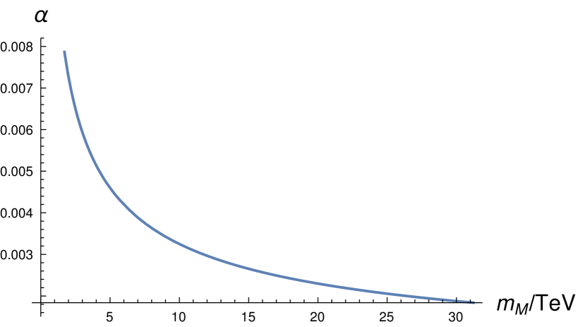
Figure 1: Muon mixing angle $\alpha$ as a function of the new muon type heavy charged lepton mass $m_{M}$.

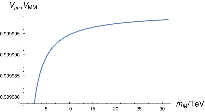
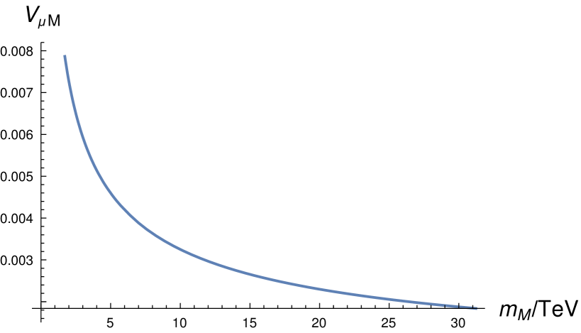
Figure 2: Diagonal (left) and non-diagonal (right) elements of the muon mixing matrix $V$ as a function of the new muon type heavy charged lepton mass $m_{M}$. Note that $V_{\mu\mu}=V_{MM}$ (see (2.13)).

3 Muon anomalous magnetic moment

The recent results from Fermilab indicate a $4.2\sigma$ deviation of the muon’s anomalous magnetic moment from its theoretical SM prediction [1],

$$\Delta a=a_{\mu}^{exp}-a_{\mu}^{SM} =451\pm 59\times 10^{-11}\,,$$ (3.1)

which improves significantly upon the result from the $g-2$ collaboration at BNL [28],

$$\Delta a_{BNL}=\left(a_{\mu}^{exp}-a_{\mu}^{SM}\right)_{BNL} =426\pm 165\times 10^{-11}\,.$$ (3.2)

In a model with an extended muon sector, a BSM contribution to $a_{\mu}$ arises [3] as

$$a_{\mu}=\frac{\xi_{\mu M}}{16\pi^{2}}\int_{0}^{1}\frac{x^{2}(1-x)+x^{2}\frac{m_{M}}{m_{\mu}}}{x(x-1)+x\frac{m_{M}^{2}}{m_{\mu}^{2}}+(1-x)\frac{m_{h^{\prime}}^{2}}{m_{\mu}^{2}}}\mathrm{d}x\,.$$ (3.3)

where

$$\xi_{\mu M}=hh^{\prime}\cos\theta\sin\theta\,.$$ (3.4)

The corresponding Feynman diagram can be found in Fig. 3. Note that we do not get a contribution from $SU(3)_{L}$ and $SU(3)_{R}$ gauge bosons as in [23] since we assume a unification scale much higher than $v^{\prime}$. In Fig. 4, the fraction $\nicefrac{{a_{\mu M}}}{{\xi_{\mu M}}}$ is shown using recent values for $\Delta a,m_{h}$ and $m_{\mu}$. We observe that the contribution to the muon anomalous magnetic moment in the considered model decreases with increasing $m_{M}$.

Figure 3: Feynman diagram contributing to $a_{\mu}$ in the model with the new muon type charged fermions.

Recalling (2.11), we obtain

$$hh^{\prime}=\frac{m^{2}_{mix}}{vv^{\prime}}\approx\frac{m_{\mu}m_{M}}{vv^{\prime}}$$ (3.5)

and therefore

$$\xi_{\mu M}(m_{M},v^{\prime},\theta) =hh^{\prime}O_{hh^{\prime}}O_{S^{0}h^{\prime}}=\frac{m_{\mu}m_{M}}{vv^{\prime}}\cos\theta\sin\theta$$ (3.6)

$$a_{\mu}(m_{M},v^{\prime},\theta) =\frac{\xi_{\mu M}(m_{M},v^{\prime},\theta)}{16\pi^{2}}\int_{0}^{1}\frac{x^{2}(1-x)+x^{2}\frac{m_{M}}{m_{\mu}}}{x(x-1)+x\frac{m_{M}^{2}}{m_{\mu}^{2}}+(1-x)\frac{m_{h^{\prime}}^{2}}{m_{\mu}^{2}}}\mathrm{d}x\,.$$ (3.7)

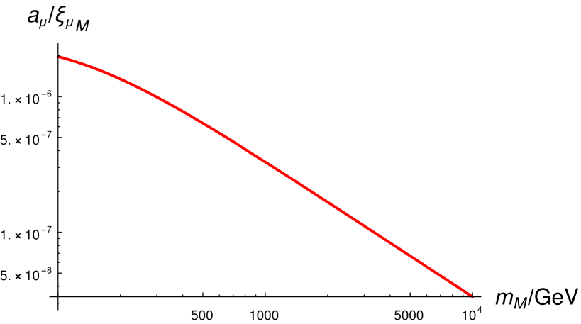
Figure 4: Muon magnetic moment $a_{\mu}$ as a function of the mass of the new muon type heavy charged lepton mass $m_{M}$ with $m_{\mu}=$105.66\text{\,}\mathrm{MeV}\text{/}$$ and $m_{H}=$125\text{\,}\mathrm{GeV}\text{/}$$.

We define

$$v^{\prime}=\eta v\,,$$ (3.8)

where $\eta$ is a proportionality constant depending on $\lambda_{mix},\lambda_{\Phi}$ and $\lambda_{S}$. For $O:=|\sin\theta\cos\theta|$, $O\in(0,0.5],$ we have

$$\xi_{\mu M}(\tilde{h},O) =O\frac{m_{\mu}\tilde{h}}{v}$$ (3.9)

$$a_{\mu}(\tilde{h},\eta,O) =\frac{\xi_{\mu M}(\tilde{h},O)}{16\pi^{2}}\int_{0}^{1}\frac{x^{2}(1-x)+x^{2}\frac{\tilde{h}\eta v}{m_{\mu}}}{x(x-1)+x\frac{(\tilde{h}\eta v)^{2}}{m_{\mu}^{2}}+(1-x)\frac{m_{h^{\prime}}^{2}}{m_{\mu}^{2}}}\mathrm{d}x\,.$$ (3.10)

In Fig. 5, the combinations of $\tilde{h}$ and $\eta$ that give a contribution to $a_{\mu}$ that fits data are shown for different values of $O$. We observe that for $\eta\gtrsim 0.1$, the coupling $\tilde{h}$ has to grow with increasing breaking scale $v^{\prime}$ in order to explain data. The effect is more pronounced for smaller mixing parameters $O$. In Fig. 6, the respective relations between $m_{M}$ and $v^{\prime}$ are shown. We observe that the larger the breaking scale $v^{\prime}$ is, the larger the required mass $m_{M}$ is in order to explain data. Conversely to the previous figure, the effect is more pronounced for larger mixing parameters $O$.

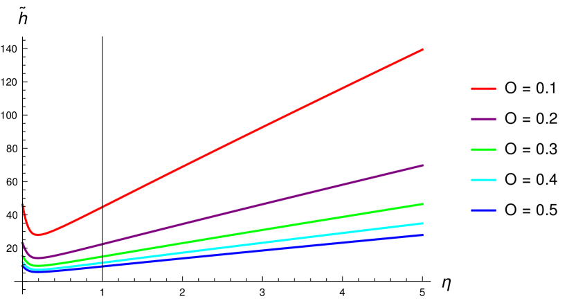
Figure 5: Yukawa coupling $\tilde{h}$ of the new muon type heavy charged leptons to the singlet scalar $S^{0}$ as a function of $\eta$ for different scalar mixing parameters $O$. The vertical line denotes where $v=v^{\prime}$.

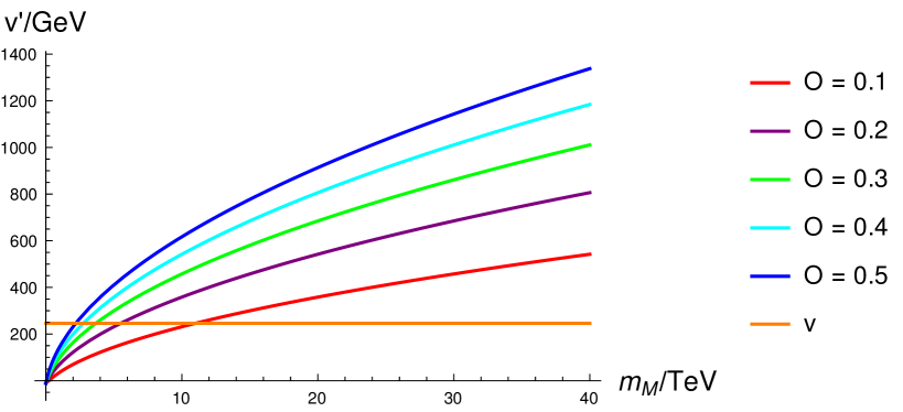
Figure 6: VEV of the singlet scalar as a function of the new muon type heavy charged lepton mass $m_{M}$ for different scalar mixing parameters $O$. The horizontal line denotes where $v=v^{\prime}$.

4 Flavor Anomalies

While lepton-flavor universality is one of the central predictions of the SM, recent experiments have observed hints for non-universality of flavor in $b\to s\ell\bar{\ell}$ and $b\to c\ell\bar{\nu}$ transitions. In the following we will discuss whether the $\mu^{f}-M^{f}$-mixing parametrized by the mixing matrix in (2.13) gives contributions to these flavor anomalies.

4.1 $R_{K^{(*)}}$

The ratios

$$R_{K^{(*)}}=\frac{\mathcal{Br}(B\to K^{(*)}\mu^{+}\mu^{-})}{\mathcal{Br}(B\to K^{(*)}e^{+}e^{-})}$$ (4.1)

test lepton flavor universality in $b$ decays via a neutral current transition (see (7)).
The SM theory prediction for $R_{K}$ is [29],[30],[31]

$$R_{K}^{SM} ={1.00\pm 0.01}\,$$ (4.2)

while the predictions for $R_{K^{*}}$ are [29], [31],[32]

$$R_{K^{*}}^{SM} =\begin{cases}0.92\pm 0.03\,,$0.045\text{\,}{\mathrm{GeV}}^{2}\text{/}$<q^{2}<$1.1\text{\,}{\mathrm{GeV}}^{2}\text{/}$\\ 1.00\pm 0.05\,,$1.1\text{\,}{\mathrm{GeV}}^{2}\text{/}$<q^{2}<$6.0\text{\,}\mathrm{GeV}\text{/}$\,.\end{cases}$$ (4.3)

The experimental results from LHCb are [33],[34]

$$R_{K}^{exp} ={0.846}^{+0.044}_{-0.041}$$ (4.4)

$$R_{K^{*}}^{exp} =\begin{cases}0.66^{+0.11}_{-0.07}\pm 0.03\,,$0.045\text{\,}{\mathrm{GeV}}^{2}\text{/}$<q^{2}<$1.1\text{\,}{\mathrm{GeV}}^{2}\text{/}$\\ 0.69^{+0.11}_{-0.07}\pm 0.05\,,$1.1\text{\,}{\mathrm{GeV}}^{2}\text{/}$<q^{2}<$6.0\text{\,}\mathrm{GeV}\text{/}$\,.\end{cases}$$ (4.5)

In the model with an extended muon sector, the terms in the Lagrangian contributing to a muonic neutral current are given by

$$\mathcal{L}_{NC}\supset\frac{e}{\sin\vartheta_{w}\cos\vartheta_{w}}Z_{\mu}\left(\overline{L}\gamma^{\mu}L(-\frac{1}{2}-\sin^{2}\vartheta_{W})+\overline{\mu_{R}}\gamma^{\mu}\mu_{R}(-\sin^{2}\vartheta_{W})\right)+eA_{\mu}Q\left(\overline{L}\gamma^{\mu}L+\overline{\mu_{R}}\gamma^{\mu}\mu_{R}\right)\,$$ (4.6)

where $L=\mu_{L},M_{L},M_{R}$. As the mixing matrix $V$ is unitary, (4.6) is already diagonal in the mass basis and thus the muon mixing does not affect $R_{K^{(*)}}$.

Figure 7: Feynman diagram for $b\to s\ell\overline{\ell}$ at 1-loop-order.

4.2 $R_{D^{(*)}}$

Deviations from lepton flavor universality in $b$ decays via a charged current transition (see (8)) are tested by the ratios

$$R_{D^{(*)}}=\frac{\mathcal{Br}(\overline{B}\to D^{(*)}\tau\overline{\nu}_{\tau})}{\mathcal{Br}(\overline{B}\to D^{(*)}\ell\overline{\nu}_{\ell})}$$ (4.7)

where $\ell=e,\mu$. The standard model expectations are [35],[36]

$$R_{D}^{SM} ={0.299\pm 0.003}$$ (4.8)

$$R_{D^{*}}^{SM} ={0.252\pm 0.003}$$ (4.9)

while the experimental results from Belle are [37]

$$R_{D}^{exp} ={0.307\pm 0.037\pm 0.013}$$ (4.10)

$$R_{D^{*}}^{exp} ={0.283\pm 0.018\pm 0.014}\,.$$ (4.11)

In the model with an extended muon sector, terms giving a contribution to the muonic charged current are given by

$$\mathcal{L}_{CC}\propto\overline{\nu_{\mu}}\not{W}^{+}\mu_{L}+\overline{\nu_{M}^{L,R}}\not{W}^{+}M_{L,R}+\overline{\mu_{L}}\not{W}^{-}\nu_{\mu}+\overline{M_{L,R}}\not{W}^{-}\nu_{M}^{L,R}$$ (4.12)

We are interested in the terms with with $\mu^{m}$ in the final state, thus

$$\mathcal{L}_{CC}\propto V_{\mu\mu}\overline{\mu^{m}}\not{W}^{-}\nu_{\mu}+V_{\mu M}\overline{\mu^{m}}\not{W}^{-}\nu_{M}^{L,R}\,,$$ (4.13)

resulting in a modified decay rate as

$$\Gamma_{M}\propto\left|V_{\mu\mu}\right|^{2}\Bigl{|}1+2\frac{V_{\mu M}}{V_{\mu\mu}}\Bigr{|}^{2}\,.$$ (4.14)

With

$$\frac{\Gamma_{b\to c\mu\overline{\nu}}(exp)}{\Gamma_{b\to c\mu\overline{\nu}}(M)}=\frac{1}{V_{\mu\mu}^{2}}\Gamma_{M}$$ (4.15)

we obtain

$$\frac{R(exp)}{R(M)}=\frac{\Gamma_{b\to c\mu\overline{\nu}}(M)}{\Gamma_{b\to c\mu\overline{\nu}}(exp)}=\frac{1}{\left|1+2\frac{V_{\mu M}}{V_{\mu\mu}}\right|^{2}}<1\,.$$ (4.16)

However, from experiments, we have

$$\frac{R(exp)}{R(\text{model})}>1\,.$$ (4.17)

Consequently, a model with an extended muon sector doesn’t give a contribution to $R_{D}^{(*)}$ that could explain the anomalies. In case that the flavor anomalies do not persist, the considered model with an extended muon sector could offer a viable explanation for $a_{\mu}$ independently of $R_{K}^{(*)}$ and $R_{D}^{(*)}$.

Figure 8: Feynman diagram for $b\to c\ell\overline{\nu}_{\ell}$ at tree level.

5 Higgs Decays

So far, we have assumed that the Higgs boson with $m_{H}\approx$126\text{\,}\mathrm{GeV}\text{/}$$ behaves just like the SM Higgs boson. However, introducing new fermions may affect the properties of the $126\text{\,}\mathrm{GeV}\text{/}$ Higgs and thereby hint at physics beyond the SM. In this section, we examine the effect of the $\mu^{f}-M^{f}$ on the decays of the Higgs boson.

5.1 Leptonic Higgs Decay

As leptonic Higgs decays to the new muon type charged lepton are kinematically forbidden, we only need to consider Higgs decays to the SM muon. The decay rate is altered due to the terms

$$\mathcal{L}\propto\underbrace{\tilde{h}(V_{\mu\mu}^{2}+V_{\mu M})}_{=:g_{hMM}}h^{0}\bar{\mu^{m}}\mu^{m}$$ (5.1)

as

$$\frac{\Gamma(h\to\mu\mu)}{\Gamma(h\to\mu\mu)_{SM}}=\Bigl{|}1+\frac{V_{\mu M}V_{\mu\mu}}{V_{\mu\mu}^{2}}\Bigr{|}^{2}\,$$ (5.2)

where $\frac{V_{\mu M}V_{\mu\mu}}{V_{\mu\mu}^{2}}\sim\mathcal{O}\left(10^{-3}\right)$. We conclude that the contribution is negligible.

5.2 $h\to\gamma\gamma$

In the SM, the main contribution to the Higgs decay to two photons comes from the diagrams with top-quarks and $W$-bosons propagating in the loop. Thus, the decay width in the SM is given by

$$\Gamma(h\to\gamma\gamma)_{SM}\propto\left|\frac{2}{v}A_{1}(\tau_{W})+\frac{2}{v}N_{c,t}Q_{t}^{2}A_{\frac{1}{2}}(\tau_{t})\right|^{2}\,,$$ (5.3)

where $A_{1}$ and $A_{\frac{1}{2}}$ are loop functions, given in A.2, $N_{c,t}=3$ is the number of color, $Q_{t}=\frac{2}{3}$ is the top quark electric charge and $\tau_{i}:=4\frac{m_{i}^{2}}{m_{h}^{2}}$.
In the model with an extended muon sector, the muon type charged lepton can propagate in the loop, thus potentially changing the Higgs to diphoton rate. Consequently, the decay rate is given by

$$\Gamma(h\to\gamma\gamma)_{M}\propto\left|\frac{2}{v}A_{1}(\tau_{W})+\frac{2}{v}N_{c,t}Q_{t}^{2}A_{\frac{1}{2}}(\tau_{t})+\frac{2g_{hM\bar{M}}}{m_{M}}Q_{M}^{2}A_{\frac{1}{2}}(\tau_{M})\right|^{2}\;.$$ (5.4)

Using

$$\frac{2g_{hM\bar{M}}}{m_{M}}=\left(V_{\mu M}^{2}+V_{\mu M}V_{MM}\right)\frac{2}{v^{\prime}}\;,$$ (5.5)

we find that the decay rate is modified as

$$\frac{\Gamma(h\to\gamma\gamma)_{M}}{\Gamma(h\to\gamma\gamma)_{SM}}=\left|1-\frac{0.2}{\eta}\left(V_{\mu M}^{2}+V_{\mu M}V_{MM}\right)\right|^{2}\,.$$ (5.6)

With $V_{\mu M}\sim 10^{-3}$, we conclude that the contribution of the muon type charged lepton to the higgs diphoton decay is negligible.

Figure 9: Feynman diagram for $h\to\gamma\gamma(Z)$ at 1-loop order.

Figure 10: Feynman diagram for $h\to\gamma\gamma(Z)$ at 1-loop order.

5.3 $h\to\gamma Z$

Finally, in a similar manner to the diphoton decay, the Higgs boson can also decay to a photon and a $Z$ boson with the main SM contribution coming from the diagrams with top-quarks and $W$-bosons propagating in the loop. The SM decay width is given by

$$\Gamma(h\to\gamma Z)_{SM}=\left|\frac{2}{v}\cot\vartheta_{W}A_{1}(\tau_{W},\lambda_{W})+N_{c,t}\frac{2}{v}\frac{2Q_{t}}{\sin\vartheta_{W}\cos\vartheta_{W}}(T_{3}^{(t)}-2Q_{t}\sin\vartheta^{2})A_{\frac{1}{2}}(\tau_{t},\lambda_{t})\right|^{2}$$ (5.7)

while the $h\to\gamma Z$-rate in our model with an extended muon sector is given by

$$\Gamma(h\to\gamma Z)_{SM}=\Big{|}\frac{2}{v}\cot\vartheta_{W}A_{1}(\tau_{W},\lambda_{W})+N_{c,t}\frac{2}{v}\frac{2Q_{t}}{\sin\vartheta_{W}\cos\vartheta_{W}}(T_{3}^{(t)}-2Q_{t}\sin\vartheta^{2})A_{\frac{1}{2}}(\tau_{t},\lambda_{t})$$

$$+\frac{2g_{hM\bar{M}}}{m_{M}}\frac{2Q_{M}}{\sin\vartheta_{W}\cos\vartheta_{W}}(2T_{3}^{(M)}-2Q_{M}\sin\vartheta^{2})A_{\frac{1}{2}}(\tau_{M},\lambda_{M})\Big{|}^{2}\,,$$ (5.8)

thus modifying the $\Gamma(h\to\gamma Z)$ as

$$\frac{\Gamma(h\to\gamma Z)_{M}}{\Gamma(h\to\gamma Z)_{SM}}=\left|1+\frac{\frac{2g_{hM\bar{M}}}{m_{M}}\frac{2Q_{M}}{\sin\vartheta_{W}\cos\vartheta_{W}}(2T_{3}^{(M)}-2Q_{M}\sin\vartheta^{2})A_{\frac{1}{2}}(\tau_{M},\lambda_{M})}{\frac{2}{v}\cot\vartheta_{W}A_{1}(\tau_{W},\lambda_{W})+N_{c,t}\frac{2}{v}\frac{2Q_{t}}{\sin\vartheta_{W}\cos\vartheta_{W}}(T_{3}^{(t)}-2Q_{t}\sin\vartheta^{2})A_{\frac{1}{2}}(\tau_{t},\lambda_{t})}\right|^{2}\,.$$ (5.9)

In the above, $T_{3}^{(i)}$ is the weak isospin of the respective lepton and $\lambda_{i}=4\frac{m_{i}^{2}}{m_{Z}^{2}}$.
Writing this expression in terms of VEVs and mixing matrix elements as previously, we obtain

$$\frac{\Gamma(h\to\gamma Z)_{M}}{\Gamma(h\to\gamma Z)_{SM}}=\left|1-\frac{0.06}{\eta}(V_{\mu M}^{2}+V_{\mu M}V_{MM})\right|^{2}\,.$$ (5.10)

As before, we conclude that the contribution is negligible.

6 Radiative Lepton Flavor Violating Decay

In general, the considered model with an extended muon sector can give contributions to radiative lepton flavor violating (LFV) decays with muons in the initial or final state (see Fig. 11). We will assume that both the SM and the model with an extended muon sector have been extended in a way that accounts for neutrino masses, with the details being irrelevant. As the flavor eigenstates of the neutrinos differ from the mass eigenstates, neutrino oscillations occur. The flavor eigenstates can be written as a sum over the neutrino mass eigenstates as

$$\ket{\nu_{\alpha}}=\sum_{k}U_{\alpha k}\ket{\nu_{k}}$$ (6.1)

where $\alpha={e,\mu,\tau}$, $k=1,2,3$ in the SM extended by neutrino masses, and $\alpha={e,\mu,\tau,M^{L},M^{R}}$, $k=1,2,3,4,5$ in the model with an extended muon sector. For simplicity, we will discuss the effects of an extended muon sector on radiative lepton flavor violating decays using the example of $\tau\to\mu\gamma$ where $\mu$ is a SM muon in its mass eigenstate. The extension to other LFV decays involving muons is straightforward. In the SM extended by neutrino masses, the LFV decay width of $\tau\to\mu\gamma$ is proportional to the PMNS matrix elements of the respective initial and final states,

$$\Gamma(\tau\to\mu\gamma)_{SM+m_{\nu}}\propto|\sum_{k=1}^{3}U_{\tau k}U^{*}_{\mu k}|^{2}$$ (6.2)

while the decay width in the model with an extended muon sector and neutrino masses is suppressed due to the additional mixing in the muon sector,

$$\Gamma(\tau\to\mu\gamma)_{SM+M+m_{\nu}}\propto|\sum_{k=1}^{5}U_{\tau k}U^{*}_{\beta k}V_{\mu\beta}|^{2}\,.$$ (6.3)

Assuming that mixing between the SM neutrinos and $\nu_{M}^{L,R}$ is small, the leading contribution of $\Gamma(\tau\to\mu\gamma)_{SM+M+m_{\nu}}$ is given by

$$\Gamma(\tau\to\mu\gamma)_{SM+M+m_{\nu}}\sim|\sum_{k=1}^{3}U_{\tau k}U^{*}_{\mu k}V_{\mu\mu}|^{2}\lessapprox\Gamma(\tau\to\mu\gamma)_{SM+m_{\nu}}\,.$$ (6.4)

We conclude that the leading contributions in both cases come from the SM lepton sector with contributions coming from the muon type lepton in the model with an extended muon sector being negligible.

Figure 11: Feynman diagram for $\ell^{\prime}\to\gamma\ell$ at 1-loop-order where $\ell^{\prime}$, $\ell$ are charged SM leptons with one of them being a muon and $\nu_{k}$ is a neutrino in its mass eigenstate.

7 Summary

In this paper we have investigated a Standard Model extension with a vectorlike lepton in the ${\cal O}(10~{}{\rm TeV})$ region and a scalar singlet that arises naturally in $E_{6}$ and Trinification models and provides an elegant and natural explanation of the recently announced measurement of the anomalous magnetic moment. We have carefully studied the model’s parameter space and checked various phenomenological implications and constraints. We find that the model cannot explain the anomalies indicating lepton flavor non-universality in the observables $R_{K(*)}$ and $R_{D(*)}$ and implies only negligible contributions to exotic Higgs decay modes. We also don’t find large contributions to charged lepton flavor violating radiative deacys such as $\mu\rightarrow e\gamma$ or $\tau\rightarrow\mu\gamma$. We conclude that it will be interesting to search for the direct production of vectorlike leptons at the LHC and at future collider experiments.

Appendix A Appendix

A.1 Higgs Decay Rates

Defining $\tau_{i}=4\frac{m_{i}^{2}}{m_{h}}^{2},i=V,f$, the diphoton decay width for a general model including spin$-1$ particles $V$ and fermions $f$ with electric charge $Q_{i}$ coupling to the Higgs is given by [38]

$$\Gamma(h\to\gamma\gamma)\propto\left|\frac{g_{hVV}}{m_{V}^{2}}Q_{V}^{2}A_{1}(\tau_{V})+\frac{2g_{hf\bar{f}}}{m_{f}}N_{c,f}Q_{f}^{2}A_{\frac{1}{2}}(\tau_{f})\right|^{2}\;.$$ (A.1)

The $h\to\gamma Z$ decay width for a general model including spin$-1$ particles $V$ and fermions $f$ coupling to the Higgs is given by [38]

$$\Gamma(h\to\gamma Z)=\left|\frac{g_{hVV}}{m_{V}^{2}}g_{ZVV}A_{1}(\tau_{V},\lambda_{V})+N_{c,f}\frac{2g_{hf\bar{f}}}{m_{f}}(2Q_{f})(g_{Zll}^{f}+g_{Zrr}^{f})A_{\frac{1}{2}}(\tau_{f},\lambda_{f})\right|^{2}$$ (A.2)

where $\lambda_{i}=4\frac{m_{i}^{2}}{m_{Z}^{2}}$ and

$$g_{Zkk}^{f}=\frac{1}{\sin\vartheta_{W}\cos\vartheta_{W}}(T_{3}^{(k,f)}-Q_{f}\sin\vartheta_{W}^{2})\,\qquad k=l,r$$ (A.3)

are the couplings of the $Z$ to left- and right-handed particles with weak isospin $T_{3}^{k,f}$, respectively.

A.2 Loop Functions

$$A_{1}(x) =-x^{2}\left(2x^{-2}+3x^{-1}+3(2x^{-1}-1)f(x^{-1})\right)$$ (A.4)

$$A_{\frac{1}{2}}(x) =2x^{2}\left(x^{-1}+\left(x^{-1}-1\right)f(x^{-1})\right)$$ (A.5)

$$A_{1}(x,y) =4(3-\tan^{2}\vartheta_{W})I_{2}(x,y)+[(1-\frac{2}{x})\tan^{2}\vartheta-(5+\frac{2}{x}]I_{1}(x,y)$$ (A.6)

$$A_{\frac{1}{2}}(x,y) =I_{1}(x,y)-I_{2}(x,y)$$ (A.7)

$$I_{1}(x,y) =\frac{xy}{2(x-y)}+\frac{x^{2}y^{2}}{2(x-y)^{2}}[f(x^{-1})-f(y^{-1})]+\frac{x^{2}y}{(x-y)^{2}}[g(x^{-1})-g(y^{-1})]$$ (A.8)

$$I_{2}(x,y) =-\frac{xy}{2(x-y)}[f(x^{-1})-f(y^{-1})]$$ (A.9)

$$f(x) =\arcsin^{2}\sqrt{x}$$ (A.10)

$$g(x) =\sqrt{x^{-1}-1}\arcsin\sqrt{x}$$ (A.11)

References

- [1] Muon Collaboration, B. Abi et al., Phys. Rev. Lett. 126, 141801 (2021).
- [2] P. Athron, C. Balázs, D. H. J. Jacob, W. Kotlarski, D. Stöckinger and H. Stöckinger-Kim, JHEP 09 (2021), 080 arXiv:2104.03691 [hep-ph].
- [3] T. W. Kephart and H. Päs, Physical Review D 65, 093014 (2002) arXiv:0102243 [hep-ph].
- [4] F. Gursey, P. Ramond, and P. Sikivie, ‘‘A Universal Gauge Theory Model Based on E6,’’ Phys. Lett. B 60 (1976) 177--180.
- [5] Q. Shafi, ‘‘E(6) as a Unifying Gauge Symmetry,’’ Phys. Lett. B 79 (1978) 301--303.
- [6] Y. Achiman and B. Stech, ‘‘Quark Lepton Symmetry and Mass Scales in an E6 Unified Gauge Model,’’ Phys. Lett. B 77 (1978) 389--393.
- [7] A. de Rujula, H. Georgi, and S. L. Glashow, ‘‘Trinification of all elementary particle forces,’’ in Fifth Workshop on Grand Unification, edited by K. Kang, H. Fried, and P. Frampton. (World Scientific, Singapore, 1984).
- [8] K. S. Babu, X.-G. He, and S. Pakvasa, ‘‘Neutrino Masses and Proton Decay Modes in SU(3) X SU(3) X SU(3) Trinification,’’ Phys. Rev. D 33 (1986) 763.
- [9] G. R. Dvali and Q. Shafi, ‘‘Gauge hierarchy, Planck scale corrections and the origin of GUT scale in supersymmetric ,’’ Phys. Lett. B 339 (1994) 241--247, arXiv:hep-ph/9404334.
- [10] G. R. Dvali and Q. Shafi, ‘‘Gauge hierarchy in and low-energy implications,’’ Phys. Lett. B 326 (1994) 258--263, arXiv:hep-ph/9401337.
- [11] T. W. Kephart and Q. Shafi, ‘‘Family unification, exotic states and magnetic monopoles,’’ Phys. Lett. B 520 (2001) 313--316, arXiv:hep-ph/0105237.
- [12] S. Willenbrock, ‘‘Triplicated trinification,’’ Phys. Lett. B 561 (2003) 130--134, arXiv:hep-ph/0302168.
- [13] J. E. Kim, ‘‘Trinification with = 3/8 and seesaw neutrino mass,’’ Phys. Lett. B 591 (2004) 119--126, arXiv:hep-ph/0403196.
- [14] J. Sayre, S. Wiesenfeldt, and S. Willenbrock, ‘‘Minimal trinification,’’ Phys. Rev. D 73 (2006) 035013, arXiv:hep-ph/0601040.
- [15] T. W. Kephart, C.-A. Lee, and Q. Shafi, ‘‘Family unification, exotic states and light magnetic monopoles,’’ JHEP 01 (2007) 088, arXiv:hep-ph/0602055.
- [16] C. Cauet, H. Päs, S. Wiesenfeldt, H. Pas, and S. Wiesenfeldt, ‘‘Trinification, the Hierarchy Problem and Inverse Seesaw Neutrino Masses,’’ Phys. Rev. D 83 (2011) 093008, arXiv:1012.4083 [hep-ph].
- [17] J. Hetzel and B. Stech, ‘‘Low-energy phenomenology of trinification: an effective left-right-symmetric model,’’ Phys. Rev. D 91 (2015) 055026, arXiv:1502.00919 [hep-ph].
- [18] J. Hetzel, Phenomenology of a left-right-symmetric model inspired by the trinification model. PhD thesis, U. Heidelberg (main), 2015. arXiv:1504.06739 [hep-ph].
- [19] G. M. Pelaggi, A. Strumia, and S. Vignali, ‘‘Totally asymptotically free trinification,’’ JHEP 08 (2015) 130, arXiv:1507.06848 [hep-ph].
- [20] K. S. Babu, B. Bajc, M. Nemevšek, and Z. Tavartkiladze, ‘‘Trinification at the TeV scale,’’ AIP Conf. Proc. 1900 no. 1, (2017) 020002.
- [21] Z.-W. Wang, A. Al Balushi, R. Mann, and H.-M. Jiang, ‘‘Safe Trinification,’’ Phys. Rev. D 99 no. 11, (2019) 115017, arXiv:1812.11085 [hep-ph].
- [22] K. S. Babu, S. Jana, and A. Thapa, ‘‘Vector Boson Dark Matter From Trinification,’’ arXiv:2112.12771 [hep-ph].
- [23] D. Raut, Q. Shafi and A. Thapa, arXiv:2201.11609 [hep-ph].
- [24] S. Kachru and E. Silverstein, Phys. Rev. Lett. 80, 4855 (1998) arXiv:9802183 [hep-th].
- [25] P. H. Frampton, Phys. Rev. D 60, 121901 (1999) arXiv:9907051[hep-th].
- [26] P. H. Frampton and T. W. Kephart, Phys. Lett. B 485, 403 (2000) arXiv:9912028[hep-th].
- [27] P. H. Frampton and T. W. Kephart, Phys. Rev. D 64, 086007 (2001) arXiv:0011186[hep-th].
- [28] H. N. Brown et al., Physical Review Letters 86, 2227–2231 (2001).
- [29] S. Descotes-Genon, L. Hofer, J. Matias, and J. Virto, Journal of High Energy Physics 2016 (2016).
- [30] C. Bobeth, G. Hiller, and G. Piranishvili, Journal of High Energy Physics 2007, 040–040 (2007).
- [31] M. Bordone, G. Isidori, and A. Pattori, The European Physical Journal C 76 (2016).
- [32] B. Capdevila, A. Crivellin, S. Descotes-Genon, J. Matias, and J. Virto, Journal of High Energy Physics 2018 (2018).
- [33] R. Aaij et al., Nature Phys. 18 (2022) no.3, 277-282 arXiv:2103.11769 [hep-ex].
- [34] R. Aaij et al., Journal of High Energy Physics 2017 (2017).
- [35] D. Bigi and P. Gambino, Physical Review D 94 (2016).
- [36] S. Fajfer, J. F. Kamenik, and I. Nišandžić, Physical Review D 85 (2012).
- [37] Belle Collaboration, G. Caria et al., Phys. Rev. Lett. 124, 161803 (2020).
- [38] M. Carena, I. Low, and C. E. M. Wagner, Journal of High Energy Physics 2012 (2012).
- [39] P. A. Zyla et al. , PTEP 2020 (2020) no.8, 083C01.