Modelling the host galaxies of binary compact object mergers with observational scaling relations
Abstract
The merger rate density evolution of binary compact objects and the properties of their host galaxies carry crucial information to understand the sources of gravitational waves. Here, we present galaxyate, a new code that estimates the merger rate density of binary compact objects and the properties of their host galaxies, based on observational scaling relations. We generate our synthetic galaxies according to the galaxy stellar mass function. We estimate the metallicity according to both the mass-metallicity relation (MZR) and the fundamental metallicity relation (FMR). Also, we take into account galaxy-galaxy mergers and the evolution of the galaxy properties from the formation to the merger of the binary compact object. We find that the merger rate density changes dramatically depending on the choice of the star-forming galaxy main sequence, especially in the case of binary black holes (BBHs) and black hole neutron star systems (BHNSs). The slope of the merger rate density of BBHs and BHNSs is steeper if we assume the MZR with respect to the FMR, because the latter predicts a shallower decrease of metallicity with redshift. In contrast, binary neutron stars (BNSs) are only mildly affected by both the galaxy main sequence and metallicity relation. Overall, BBHs and BHNSs tend to form in low-mass metal-poor galaxies and merge in high-mass metal-rich galaxies, while BNSs form and merge in massive galaxies. We predict that passive galaxies host at least %, %, and % of all BNS, BHNS and BBH mergers in the local Universe.
keywords:
gravitational waves – black hole physics – stars: neutron – galaxies: star formation – methods: numerical1 Introduction
The third gravitational wave transient catalog (GWTC-3) of the LIGO–Virgo–KAGRA collaboration (LVK) contains 90 gravitational-wave (GW) event candidates (Abbott et al., 2021a). From this growing number of detections, we can extract several astrophysical properties of binary compact objects (BCOs), such as their masses, spins and merger rates. From GWTC-3, the LVK inferred a local merger rate density Gpc-3 yr-1, Gpc-3 yr-1 and Gpc-3 yr-1 for binary black holes (BBHs), black hole-neutron star binaries (BHNSs) and binary neutron stars (BNSs), respectively (Abbott et al., 2021b). In the case of BBHs, it is even possible to reconstruct the evolution of the merger rate with redshift with . Abbott et al. (2021b) find at 99.6% credibility, indicating that the BBH merger rate density increases with redshift. Thanks to the next-generation ground-based GW detectors, Einstein Telescope (Punturo et al., 2010) and Cosmic Explorer (Reitze et al., 2019), we will be able to reconstruct the redshift evolution of the BBH merger rate up to redshift or even higher (Kalogera et al., 2019, 2021; Maggiore et al., 2020).
While the merger rate provides crucial insights about the formation of BCOs (e.g., Dominik et al., 2013; Belczynski et al., 2016; Mapelli et al., 2017, 2018a; Baibhav et al., 2019; Neijssel et al., 2019), the properties of their host galaxies (HGs) represent another fundamental piece of information (e.g., Perna & Belczynski, 2002; Belczynski et al., 2006; O’Shaughnessy et al., 2010; Lamberts et al., 2016; Schneider et al., 2017; Mapelli et al., 2018b; Artale et al., 2019, 2020a; Artale et al., 2020b). Also, the identification of the host galaxy is crucial to reduce the uncertainties on the measure of the Hubble constant from GW sources (Abbott et al., 2017b; Fishbach et al., 2019; Gray et al., 2020; Jin et al., 2021; Leandro et al., 2022), and to successfully use BCOs as tracers of large scale structures (Vijaykumar et al., 2020; Adhikari et al., 2020; Libanore et al., 2021, 2022; Mukherjee et al., 2021; Cigarrán Díaz & Mukherjee, 2022).
At present, only the HG of the BNS merger GW170817 (Abbott et al., 2017a; Abbott et al., 2017c; Goldstein et al., 2017; Savchenko et al., 2017; Margutti et al., 2017; Coulter et al., 2017; Soares-Santos et al., 2017; Chornock et al., 2017; Cowperthwaite et al., 2017; Nicholl et al., 2017; Pian et al., 2017; Alexander et al., 2017), the elliptical galaxy NGC 4993, has been identified beyond any reasonable doubt (Levan et al., 2017; Im et al., 2017; Ebrová et al., 2020; Kilpatrick et al., 2022). The main obstacle to the successful identification of the HG is represented by the sky localisation uncertainties of GW detectors, currently being of the order of several ten square degrees (Abbott et al., 2018).
Several criteria to rank the galaxies within the sky localisation region have been proposed, in order to optimize the search for electromagnetic counterparts (e.g., Kopparapu et al., 2008; Arcavi et al., 2017; Ducoin et al., 2020; Stachie et al., 2020; Artale et al., 2020b; Ashkar et al., 2021a, b; Kovlakas et al., 2021; Perna et al., 2022). Furthermore, several authors studied the properties of the HGs on a theoretical ground; most of them interface the outputs of cosmological simulations with catalogs of compact objects, either obtained through population-synthesis or phenomenological models (e.g., O’Shaughnessy et al., 2017; Schneider et al., 2017; Mapelli et al., 2017; Toffano et al., 2019; Artale et al., 2019, 2020a; Artale et al., 2020b; Adhikari et al., 2020; Mandhai et al., 2022; Chu et al., 2021; Rose et al., 2021; Perna et al., 2022; Mukherjee & Moradinezhad Dizgah, 2021). These previous works suggest that the BCO merger rate per galaxy correlates with the stellar mass and star formation rate (SFR) of the HG (e.g., Artale et al., 2020a).
Here, we present a new fast numerical tool to estimate the cosmic merger rate density and to characterize the properties of the HGs of BCO mergers. Our new code galaxyate exploits the main observational scaling relations (galaxy stellar mass function, SFR distribution, mass-metallicity relation, and fundamental-metallicity relation) to generate the distribution of galaxy masses, SFR and metallicity across cosmic time (Boco et al., 2019; Safarzadeh & Berger, 2019; Safarzadeh et al., 2019; Elbert et al., 2018; Chruslinska & Nelemans, 2019; Chruślińska et al., 2020; Chruślińska et al., 2021). We derive the properties of the BCOs, and especially their delay times111We define the delay time as the time elapsed from the formation of the progenitor binary star to the merger of the BCO. , from up-to-date binary population synthesis simulations (Santoliquido et al., 2021). galaxyate is very flexible and can read catalogs from phenomenological models of BCO mergers as well.
Unlike models based on computationally expensive cosmological simulations, galaxyate can be used to probe the parameter space of BCO mergers: a single model requires CPU hours on a single core. With respect to similar codes based on observational scaling relations (e.g., Boco et al., 2019; Safarzadeh & Berger, 2019; Safarzadeh et al., 2019; Elbert et al., 2018), we have developed a new algorithm that is able to differentiate between the galaxy in which a BCO forms [hereafter, formation galaxy (FG)], and the galaxy where the BCO merges after the delay time [hereafter, host galaxy (HG)]. In fact, the properties of the FG and those of the HG can be very different from each other, not only because galaxies merge with other galaxies across the cosmic time, but also because the same galaxy can evolve significantly during the BCO delay time, changing its mass, SFR and metallicity. Our new algorithm evaluates a conditional probability that the HG of a BCO has mass and star formation rate , given the mass of the FG (), its SFR (), the formation and the merger redshift of the BCO ( and , respectively). To calculate this probability, we use the galaxy merger tree extracted from the eagle cosmological simulation with a (100 cMpc)3 volume (Schaye et al., 2015; Qu et al., 2017), but our formalism can be easily generalized to other merger trees.
The paper is organized as follows: in Section 2.1, we present the main formalism we adopted in our population-synthesis code mobse (Giacobbo & Mapelli, 2018a); Section 2.2 describes the observational scaling relations adopted in galaxyate; Sections 2.3 and 2.4 discuss the method to evaluate the merger rate density and the conditional probability, respectively. Section 3 presents our main results. We discuss the implications of our new methodology in Section 4, and draw our main conclusions in Section 5.
2 Methods
Here, we describe our new code galaxyate, which calculates the merger rate evolution of BCOs and the properties of their host galaxies, based on population-synthesis simulations and observational scaling relations. galaxyate is an upgrade of our code cosmoate (Santoliquido et al., 2020, hereafter S20). Appendix A is a short description of the main features of cosmoate. Table 1 summarises the parameters included in galaxyate and discussed in the following sections.
2.1 Binary compact objects (BCOs)
The open-source population synthesis code mobse (Mapelli et al., 2017; Giacobbo & Mapelli, 2018b) is an upgraded and customized version of bse (Hurley et al., 2000, 2002). With respect to the original version of bse, mobse includes an up-to-date formalism for stellar winds (Giacobbo & Mapelli, 2018b), and several new models for the outcome of electron-capture (Giacobbo & Mapelli, 2019), core-collapse (Fryer et al., 2012) and pair-instability supernovae (Spera & Mapelli, 2017; Mapelli et al., 2020). Here, we assume the rapid core-collapse supernova model (Fryer et al., 2012), which enforces a mass gap between the maximum mass of a neutron star (2 M⊙) and the minimum mass of a black hole (5 M⊙). Finally, we model natal kicks of compact remnants (both neutron stars and black holes) as , where is the mass of the compact object, is the mass of the ejecta, and is a random number following a Maxwellian distribution with one-dimensional root-mean square km s-1 (Giacobbo & Mapelli, 2020), inspired from the proper motions of Galactic young pulsars (Hobbs et al., 2005). mobse itegrates the main binary evolution processes (wind mass transfer, Roche lobe overflow, common envelope, magnetic braketing, equilibrium tides and GW decay) as described in Hurley et al. (2002). We refer to Giacobbo & Mapelli (2018b) for further details on mobse.
For the runs presented in this paper, we have used three different models, with three different values of the common-envelope parameter 3 and 5 (hereafter, , and ). For each run, we have simulated 12 different metallicities: , 0.0004, 0.0008, 0.0012, 0.0016, 0.002, 0.004, 0.006, 0.008, 0.012, 0.016, and 0.02. For metallicities (), we have simulated () massive binary stars per each model.
The primary mass of each binary star follows a Kroupa initial-mass function (IMF, Kroupa, 2001) with minimum (maximum) mass (150) M⊙. We derive the mass ratio as with , the orbital period from with and the eccentricity from (Sana et al., 2012). Appendix B discusses some of the main features of these population-synthesis simulations (merger efficiency and delay time distribution).
2.2 Observational scaling relations
Hereafter, we call formation galaxy (FG) the galaxy where the stellar progenitors of the BCO form, and host galaxy (HG) the galaxy where the BCO merges via GW emission. We describe each FG with three parameters: the galaxy stellar mass (), star-formation rate (SFR) and a log-normal distribution of metallicities. This is the minimum amount of information that allows us to understand the link between galaxy properties and compact object mergers. In order to create a population of star-forming galaxies in which our compact objects form, we sample , SFR and the average galaxy metallicity from three different distributions, based on observational scaling relations.
2.2.1 Stellar mass function of star-forming galaxies
The stellar mass function of star-forming galaxies is given in its simplest form as a Schechter function (Schechter, 1976):
| (1) |
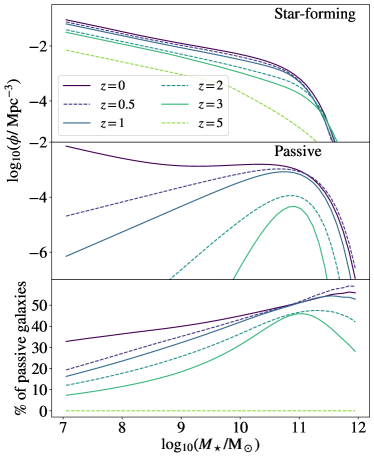
where is the normalisation, and is the stellar mass at which the Schechter function bends, changing from a single power law with slope at low masses to an exponential cut-off at high masses. We adopted the galaxy stellar-mass function (GSMF) derived in Chruslinska & Nelemans (2019), where the authors made an average of various GSMFs defined in the same redshift bin (see Table 1 of Chruslinska & Nelemans 2019). Figure 1 (upper panel) shows the resulting GSMF.
At each formation redshift, we sample a number of star-forming galaxies proportional to the galaxy number density, defined as the numerical integral of the GSMF between a minimum and a maximum stellar mass. In this way, similarly to what happens in cosmological simulations, we fixed the comoving volume . We choose this volume as a good compromise between the computational cost of our models and the statistics of high-mass galaxies in the box. In Appendix C, we discuss the impact of this choice on our results.
In the sampling procedure, we assume a maximum stellar mass M⊙. The minimum stellar mass of the GSMF is highly uncertain, especially at high redshift (Conselice et al., 2016). To this regard, we varied the minimum stellar mass M⊙ to explore the impact of this parameter on our results. In Appendix D, we show that the minimum mass has a mild impact on the merger rate density in the local Universe. For the following results, we adopted M⊙ as a fiducial value. We consider the redshift range between and 8. At higher redshift, the observations are too scanty to confidently extrapolate the GSMF.
2.2.2 Star formation rate (SFR)
Galaxies can be classified in three main groups based on their SFR. (i) The majority of galaxies belong to the so-called galaxy main sequence: they follow a tight relation between stellar mass and SFR at any redshift (Daddi et al., 2007; Speagle et al., 2014; Rodighiero et al., 2015; Schreiber et al., 2015; Pantoni et al., 2019; Lapi et al., 2020; Leja et al., 2021; Popesso et al., 2022). (ii) A second group of galaxies, the starburst galaxies, have higher SFR with respect to the main sequence (Rodighiero et al., 2011; Caputi et al., 2017). The main sequence and starburst galaxies form the population of star-forming galaxies. (iii) The third group of galaxies consists in the passive (or quenched) galaxies, which have, on average, a lower SFR with respect to the main sequence (Renzini & Peng, 2015; Bisigello et al., 2018; Santini et al., 2021). At low redshift, passive galaxies are the dominant population: they contain up to % of the total stellar mass in the local Universe (Moffett et al., 2016).
In galaxyate, we describe the star-forming galaxy distribution in SFR at fixed redshift and stellar mass with a double log-normal distribution (Daddi et al., 2007; Rodighiero et al., 2011; Sargent et al., 2012; Béthermin et al., 2012; Schreiber et al., 2015; Ilbert et al., 2015; Schreiber et al., 2015). One of the two log-normal distributions is centered on the galaxy main sequence, the other on the starburst sequence (Boco et al., 2021):
| (2) | |||
where () is the average SFR of the main sequence (starburst galaxies), () is the standard deviation of the main sequence (starburst) galaxies, and (Sargent et al., 2012). We define the starburst sequence as with dex (Sargent et al., 2012). These values are obtained expressing the SFR in M⊙ yr-1.
We compared two definitions of the galaxy main sequence : the definition given in Speagle et al. (2014, hereafter S14) and Boogaard et al. (2018, hereafter B18). The definition of galaxy main sequence by S14 is
| (3) |
where is age of the Universe in Gyr and the galaxy stellar mass in M⊙. The definition of B18 is
| (4) |
where M⊙ and . Equation 4 has been estimated considering the Chabrier IMF (Chabrier, 2003); thus, we shifted the SFR normalisation to make it consistent with our default Kroupa IMF (Kroupa 2001; see Table B1 in Chruslinska & Nelemans 2019 for more details about the conversion). The dispersion around the main sequence is another debated quantity. We assume dex for S14 (Sargent et al., 2012) and dex for B18 (Chruslinska & Nelemans, 2019).
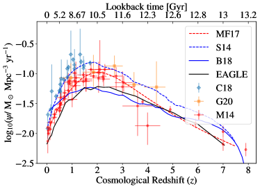
After sampling a number of galaxies from the GSMF and assigning them the SFR as described above, we can derive the total cosmic SFR density, by simply evaluating the average SFR over the population of galaxies and multiplying it by the galaxy number density at each redshift. Figure 2 shows different resulting cosmic SFR densities depending on the definition of the main sequence, and compares them to observational data. The star formation history we obtain adopting the results of S14 is in agreement with some of the most recent data points (Casey et al., 2018) and is slightly higher than the fit by Madau & Fragos (2017). In contrast, the results of B18 lie below most observational data in the redshift range , across cosmic noon. Hence, the models by S14 and B18 allow us to compare two different evolutions of the star formation history, in terms of normalisation and redshift evolution. In the same figure, we also show the cosmic SFR density from the eagle cosmological simulation with a (100 cMpc)3 volume (Furlong et al., 2015). The cosmic SFR density obtained adopting the results of B18 is close to the one evaluated with the eagle especially at high redshift ().
2.2.3 Metallicity distribution
For each galaxy, we sample an average metallicity from observational scaling relations. Two main scaling relations have been proposed between the metallicity and other galaxy properties: the mass metallicity relation (MZR, Tremonti et al., 2004; Kewley & Ellison, 2008; Maiolino et al., 2008; Mannucci et al., 2009; Magnelli et al., 2012; Zahid et al., 2014; Genzel et al., 2015; Sanders et al., 2020) and the fundamental metallicity relation (FMR, Mannucci et al., 2010, 2011; Hunt et al., 2012; Hunt et al., 2016; Curti et al., 2020; Sanders et al., 2020). The MZR is a correlation between metallicity and stellar mass, based on observations of galaxies with stellar mass in the range M⊙ and redshift (Tremonti et al., 2004; Zahid et al., 2014). In general, at fixed stellar mass the MZR predicts a steep decline in towards higher redshifts. Some earlier works (e.g., Maiolino et al., 2008; Mannucci et al., 2009; Magnelli et al., 2012) found a slow evolution of the MZR out to but a very sharp decline of about dex in between and . Extrapolating this trend at , we expect a rapid decrease of the average galaxy metallicity in the early Universe.
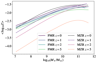
The FMR is a three-parameter relation among stellar mass, SFR and metallicity. According to the FMR, the metallicity decreases at increasing SFR, for a fixed stellar mass (Mannucci et al., 2010; Hunt et al., 2016). The FMR is thought to be almost redshift independent222Recent data from the Early Release Observations program of the James Webb Space Telescope suggest that the FMR might hold up to redshift (Curti et al., 2022)., as confirmed by observations out to (Mannucci et al., 2010). The redshift is not a parameter of the FMR, and the metallicity evolution with redshift at fixed stellar mass is entirely explained with the redshift evolution of the SFR described by the main sequence (see Section 2.2.2). This results in a shallow decline of with redshift at fixed stellar mass. Therefore, while the redshift evolution of the FMR and MZR at is similar, the evolution of the two relations becomes completely different at (Fig. 3). We refer to Section 3 of Boco et al. (2021) for a thorough discussion about the tension between the two metallicity distributions.
In the following, we will consider both MZR and FMR. To implement the MZR, we use the same definition as in Section 3.2 of Chruslinska & Nelemans (2019). For the FMR, we use the definition in Equation 2 of Mannucci et al. (2011).
Both metallicity relations are usually expressed in terms of the relative abundance of oxygen and hydrogen, . We need to convert this quantity to the total mass fraction of heavy elements , since our stellar-evolution models depend on (see Section 2.1). We assumed = 0.0153 and (Caffau et al., 2011). Other choices of the solar metallicity value result in a different normalization of the merger rate density curve (Appendix E).
Observations show that at a given stellar mass, there is an intrinsic scatter around both the MZR and FMR (Tremonti et al., 2004; Kewley & Ellison, 2008; Zahid et al., 2014; Chen et al., 2022). Thus, we assumed a log-normally distributed scatter around the mean metallicity given by both the MZR and FMR. We considered a spread dex for both relations. Furthermore, we calculate the metallicity of single stars assuming a metallicity gradient inside each galaxy, that is the metallicity of single stars is log-normally distributed around the mean metallicity of the galaxy with dex (Chruslinska & Nelemans 2019; see also Sánchez et al. 2014 and Sánchez-Menguiano et al. 2016).
Figure 3 shows the MZR and the FMR averaged over the SFR for six different redshift bins. While at the two relations give almost identical results, at the MZR yields a rapid evolution of the metallicity, resulting in much lower values than those obtained from the FMR.
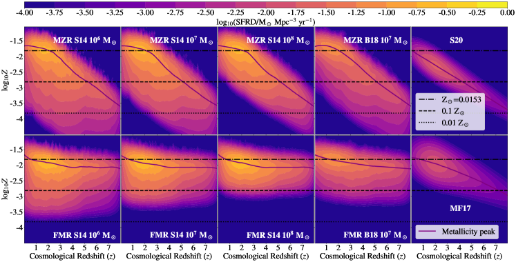
Figure 4 shows the resulting metallicity-dependent SFR density, SFRD, for each of the aforementioned models. Both the FMR and MZR produce a non-negligible fraction of metal-poor star formation (), both at high and low redshift. The fraction of metal-poor star formation increases if we assume lower values of , because smaller galaxies are also more metal poor. The metallicity associated with the highest value of the SFRD drops at high redshift if we assume the MZR or the metallicity model in Santoliquido et al. (2020), while it decreases very mildly for the FMR, in agreement with Chruślińska et al. (2021) and Boco et al. (2021).
2.2.4 Passive galaxies
In our model, we generate the mass distribution of passive galaxies from the GSMF by Ilbert et al. (2013), by adopting a double Schechter function (Pozzetti et al., 2010):
| (5) |
where the parameters and depend on redshift and are defined as in Table 2 of Ilbert et al. (2013). We linearly interpolated them between redshift bins at . Ilbert et al. (2013) show that the number density of passive galaxies rapidly drops at . Hence, in our model we assume that the number of passive galaxies is zero at .
The middle panel of Figure 1 shows the stellar mass density of passive galaxies for some redshift bins. The lower panel of the same Figure shows the percentage of passive galaxies with respect to star-forming galaxies as a function of mass for the same redshift bins. Passive galaxies represent the majority of galaxies in the local Universe at high mass ( M⊙, Moffett et al. 2016; McLeod et al. 2021). There are several ways in the literature to define passive galaxies and the resulting population can show different properties based on the chosen definition (see, e.g., Donnari et al., 2021). In our fiducial definition, we assume that passive galaxies have a value of the SFR at least one dex below the main sequence, for a given stellar mass (Donnari et al., 2019). For each passive galaxy, we extract a SFR value uniformly distributed between SFR and SFR. We assume a fixed value for SFR M⊙ yr-1, since it is unlikely that passive galaxies with M⊙ have lower SFR (Renzini & Peng, 2015). We assume , where is given by either Equation 3 (S14) or Equation 4 (B18) depending on which main sequence we assume, is the dispersion around the main sequence, and . Thus in the case of S14 (B18) (3). With this definition of , passive galaxies have maximum SFR dex below the main sequence. We estimate the average metallicity of passive galaxies either with the MZR or the FMR.
Here, we assume for simplicity that a passive galaxy cannot be the FG of the stellar progenitors of BCO mergers. This is a reasonable assumption, because the total SFR happening in passive galaxies in the local Universe is % of the total SFR. However, BCO mergers can take place in passive galaxies, because the delay time between the formation and the merger of a binary system can be several Gyr long: the FG might become a passive galaxy during and/or might merge together with a passive galaxy.
2.3 Merger rate density
To evaluate the merger rate density we proceed in a similar way as in Mapelli et al. (2017) (see also Mapelli et al. 2018a; Artale et al. 2019). At each time step , we associate to each galaxy in our sample a total mass of newly formed stars, by randomly sampling a population of stars with total zero-age main sequence mass from our population synthesis simulations. The metallicity distribution of these randomly sampled stars is the same as the metallicity distribution of the entire FG333This might overestimate the contribution of metal-poor stars, as newly born stars are generally more metal-rich than previous star formation episodes (e.g., Peeples et al., 2014). at redshift . This procedure allows us to associate the BCOs that form from this stellar population in our mobse simulations to their FG at a given formation redshift. Hereafter, we indicate with () the time (redshift) at which the progenitor stars of a BCO are associated with their FG. Each BCO merges at a time , which is estimated as . Here, both and are expressed in terms of look-back times, while is the delay time.
To evaluate the global cosmic merger rate density at a given redshift , we simply divide the total number of mergers happening at in all the considered galaxies, by the total comoving volume . For each considered galaxy, we also calculate a merger rate per galaxy , i.e. the number of compact objects merging in that galaxy per unit time.
2.4 Host galaxy (HG)
According to our definition, the HG of a BCO is the galaxy where the BCO merges. The HG can be the same as the FG, if the binary system forms and merges in the same galaxy, but it can also be different from the FG, if for example the FG has undergone galaxy-galaxy mergers by the time the two compact objects reach coalescence. Furthermore, even if the BCO forms and merges in the same galaxy, the mass, SFR and metallicity of the galaxy might change significantly after .
To reconstruct the merger history of galaxies in galaxyate we used the information from a merger tree. A merger tree encodes the entire assembly history and property evolution of each single galaxy across cosmic time (e.g., McAlpine et al., 2016; Qu et al., 2017). Here, we show the results of the merger trees taken from the eagle cosmological simulation (Schaye et al., 2015), but galaxyate can use any other possible merger trees obtained from cosmological simulations or semi-analytical models.
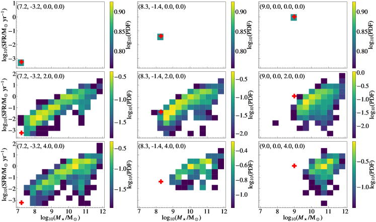
One of the main purposes of our new approach is to build a fast tool, thus we compressed the information contained in multiple merger trees, by evaluating the conditional probability , i.e. the probability that the HG of the BCO merger has mass and star formation rate , given the mass () and SFR () of the FG, and given the formation () and merger redshift () of the BCO. We evaluate the conditional probability in an empirical way, directly from the merger trees. We count the number of galaxies at a fixed that are inside each bin in the plane, by keeping fixed the condition on , and . Figure 5 shows some examples of this conditional probability, in which we compare different values of the formation redshift and different properties of the FGs. If the FG has no time to evolve between the formation and merger of the BCO (short ), the properties of the HG remain the same (upper row) as those of the FG, while if the FG has more time to evolve (long ) then the HG can be very different from the FG (lower rows).
Once we have defined the conditional probability, we sample one HG for each FG. Thereafter, we link each sampled HG from the merger trees to one and only one galaxy obtained through the observational scaling relations, considering both star-forming galaxies (Section 2.2) and passive galaxies (Section 2.2.4). Finally, to calculate the merger rate per galaxy at a given merger redshift , we sum up all the mergers of compact objects formed at any and merging at in the same galaxy.
The conditional probabilities in Figure 5 show that, in some cases, the stellar mass of the HG might be smaller than the stellar mass of the FG. This happens for two reasons. In most cases, different physical mechanisms such as strong galactic outflows or galaxy interactions producing tidal stripping can reduce the stellar mass of the galaxies (see e.g., Mac Low & Ferrara, 1999; Efstathiou, 2000; Hopkins et al., 2012). In other cases, the subfind algorithm might misclassify the star particles belonging to a given galaxy. This issue is more common at the pericenter of a subhalo orbiting a larger halo (see e.g., Muldrew et al., 2011; Knebe et al., 2011).
| Section | Parameter/Model | Value(s)/Choice(s) | Reference(s) |
| 2.1 | Core Collapse SN | Rapid | Fryer et al. (2012) |
| Natal Kicks | Giacobbo & Mapelli (2020) | ||
| Common Envelope | 1, 3 and 5 | Webbink (1984) | |
| Common Envelope | Depends on star properties | Claeys et al. (2014) | |
| Primary star IMF | Kroupa with M⊙ | Kroupa (2001) | |
| Mass ratio | Sana et al. (2012) | ||
| Orbital period | Sana et al. (2012) | ||
| Eccentricity | Sana et al. (2012) | ||
| Progenitor metallicity | Giacobbo & Mapelli (2018a) | ||
| 2.2.1 | Star-forming GSMF | Single Schechter | Chruslinska & Nelemans (2019) |
| M⊙ | Conselice et al. (2016) | ||
| constant, varying with | Chruslinska & Nelemans (2019) | ||
| 8 | Ilbert et al. (2013) | ||
| 2.2.2 | Sargent et al. (2012) | ||
| S14; B18 | Speagle et al. (2014); Boogaard et al. (2018) | ||
| , 0.3 | Sargent et al. (2012); Chruslinska & Nelemans (2019) | ||
| Sargent et al. (2012) | |||
| + | Sargent et al. (2012) | ||
| Sargent et al. (2012) | |||
| 2.2.3 | Metallicity relation | MZR; FMR | Chruslinska & Nelemans (2019); Mannucci et al. (2011) |
| 0.0153 | Caffau et al. (2011) | ||
| 0.05; 0.15; 0.30 | Boco et al. (2021) | ||
| 0.00001; 0.14; 0.30 | Chruslinska & Nelemans (2019) | ||
| Metallicity calibration | Photoionization models; based | Maiolino et al. (2008); Curti et al. (2020) | |
| 2.2.4 | Passive GSMF | Double Schechter | Ilbert et al. (2013) |
| 3 | Ilbert et al. (2013) | ||
| 1 dex below the adopted MS | Donnari et al. (2019) | ||
| M⊙ yr-1 | Renzini & Peng (2015) | ||
| 2.4 | Merger trees | eagle | Schaye et al. (2015) |
3 Results
3.1 Merger rate density
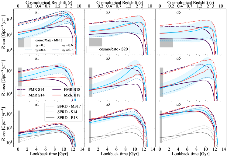
Figure 6 shows the evolution of the merger rate density for three different values of the parameter, for the two main sequence models (B18 and S14) and for the two metallicity relations (FMR and MZR). In this Figure, we also compare the results obtained with cosmoate (Appendix A) and those obtained with the new code galaxyate. For each value of the common envelope efficiency , galaxyate produces a higher local merger rate density of BBHs and BHNSs with respect to the model MF17, that we obtained with cosmoate assuming the average metallicity evolution from Madau & Fragos (2017) and a metallicity spread . This springs from the interplay of two factors. First, BBHs and BHNSs merge more efficiently if they have metal-poor progenitors in our population-synthesis models (Appendix B). Second, the SFRD distribution of galaxyate yields a longer tail of low-metallicity star formation at different redshifts with respect to cosmoate (Figure 4). The differences between the BBH merger rate density obtained with galaxyate and cosmoate (model M17) can be reconciled by assuming a larger metallicity spread in cosmoate.
The dependence of the BBH/BHNS merger rate on metallicity also appears when we vary both the main sequence definition and the metallicity relation. We have already seen that with B18 the SFR density at redshift is dex lower with respect to S14 (Figure 2). Thus, B18 quenches the formation of BBHs and BHNSs at high redshift. As a result, the merger rate density of BBHs evaluated with B18 and is times lower with respect to S14 in the local Universe.
The merger rate density of BBHs and BHNSs in the local Universe is almost the same if we adopt the MZR or the FMR. However, the two scaling relations (MZR and FMR) produce a completely different slope of the merger rate density of BBHs at . For , the merger rate density of BBHs almost decreases between , if we assume the FMR. This happens because the case with has the longest delay times (Appendix B) and the FMR yields only a mild decrease of the average metallicity with redshift (Figure 3).
In contrast, the merger rate density of BNSs does not depend on the adopted metallicity relation. Figure 6 (lower panel) shows the three cosmic SFR densities we took in account in this work. The merger rate density of BNSs approximately scales with the adopted cosmic SFR density, because in our population-synthesis models the BNSs are almost independent of metallicity and their delay times are predominantly short (e.g., Dominik et al., 2012, 2013; Klencki et al., 2018; Mapelli et al., 2018a, 2019; Neijssel et al., 2019; Santoliquido et al., 2021). In Appendix D, we also discuss the impact of the minimum galaxy stellar mass on the merger rate density.
The merger rate density of BNSs and BHNSs is within the 90% credible interval estimated by the LVK with GWTC-3 (Abbott et al., 2021b) for all considered assumptions, while the merger rate density of BBHs predicted by our models is higher than the LVK range. This discrepancy is the consequence of several factors. Firstly, here we assumed that all BBHs form via unperturbed binary evolution. Considering alternative channels might significantly affect the merger rate evolution (e.g., Mapelli et al., 2022). Furthermore, current binary evolution models might overestimate the merger rate of BBHs and its dependence on metallicity, because of the large uncertainties they are affected by (e.g., Gallegos-Garcia et al., 2021; Belczynski et al., 2022). Finally, the measurement of gas and star metallicity is affected by large uncertainties, especially at high redshift (e.g., Maiolino & Mannucci, 2019).
The merger rate density of BCOs likely extends to a redshift higher than the maximum value we considered in this work (). Here, we do not consider because we prefer to avoid to arbitrarily extrapolate the observational relationships at higher redshift. Furthermore, the merger rate density at is likely dominated by population III stars (e.g., Inayoshi et al., 2017; Liu & Bromm, 2021; Ng et al., 2021; Tanikawa et al., 2021), which are not included in our formalism. We will include them in a follow-up study.
3.2 Formation and host galaxies across cosmic time
In this Section, we look at the distribution of HG properties, namely stellar mass, SFR and metallicity. We compare them with the distribution of FGs. For the sake of brevity, we show the results only for the definition of galaxy main sequence in B18.
3.2.1 Stellar Mass
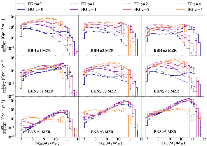
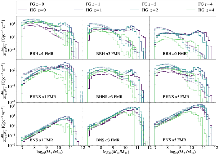
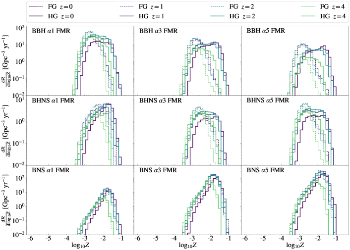
Figures 7 and 8 show the mass distribution of FGs (dashed lines) and HGs (solid lines) for the MZR and the FMR, respectively. The time elapsed between compact-object formation and merger spans from a few Myr to several Gyr (Appendix B). Hence, the HG might show significantly different properties with respect to the FG, not only because the original FG might have merged into a larger galaxy, but also because the FG might have drastically evolved (in terms of mass, SFR and metallicity) from the formation to the merger epoch of the BCO.
In the case of BNSs, the mass of the HG is always very similar to that of the FG, because BNSs merge with a short delay time and are not affected by metallicity. In contrast, the FGs of BBHs and BHNSs tend to be less massive than the HGs. This happens because many FGs merge with other galaxies by the time of the BBH/BHNS coalescence. The HGs in the local Universe are more massive than in any other previous epochs.
The fraction of high-mass HGs increases with increasing . In fact, corresponds to longer delay times on average. If the delay times are longer, the FGs have more time to merge with other galaxies and form more massive HGs. On the other hand, both Figure 7 and 8 show that a large fraction of BBH HGs are low-mass galaxies. This is more important for , which corresponds to shorter delay times. Hence, the HG mass distribution is shaped by the delay time distribution of compact objects, consistently with the result of previous authors (e.g., Mapelli et al., 2018a; Artale et al., 2019, 2020a; McCarthy et al., 2020).
The HG mass distributions of both BBHs and BHNSs depend on the adopted metallicity model. At the normalisation of the distribution is higher if we consider the MZR. This was also evident by looking at Figure 6, where at the MZR yields many more BBH mergers than the FMR.
Finally, the HGs of BNSs tend to be more massive than the HGs of both BHNSs and BBHs, at least at . The reason is that BNSs are insensitive to metallicity, while BHNSs and BBHs form predominantly in metal-poor (hence, smaller) galaxies. Both the FMR and the MZR predict that metal-poor galaxies are generally less massive than metal-rich ones.
3.2.2 Star formation rate (SFR)
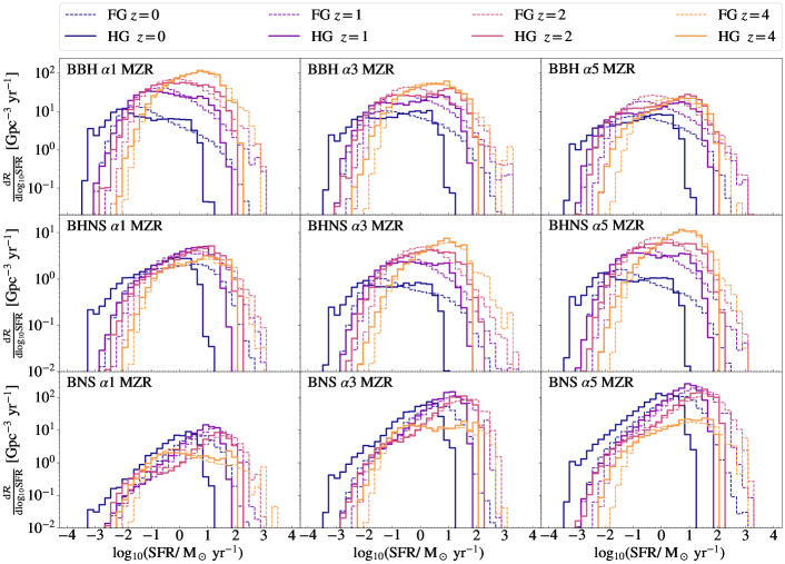
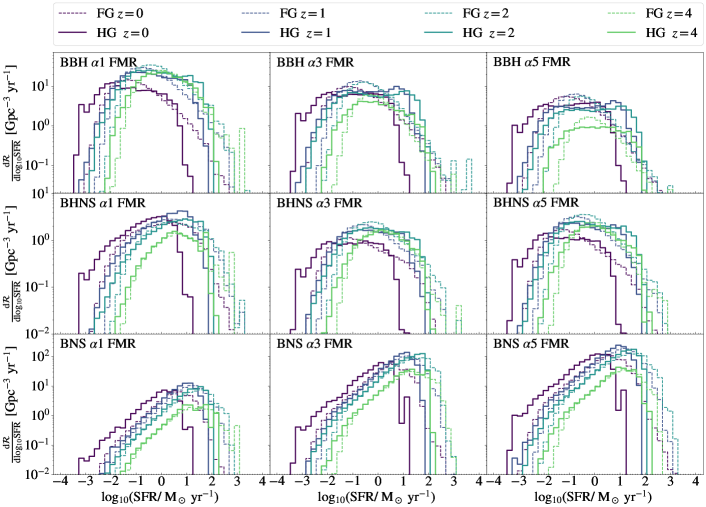
We show the SFR distribution of FGs and HGs in Figure 9 for the MZR and Figure 10 for the FMR. At lower redshifts, compact objects tend to form and merge in galaxies with lower SFR. The reason is that low-redshift galaxies have lower SFR on average, as shown in Figure 2. At higher redshift (), the SFR distribution of FGs and HGs are very similar, since the delay times are short.
At , the SFR of FGs and HGs of BBHs peaks at lower values when we assume the FMR than in the case of the MZR. The reason is that the metallicity of massive and high star-forming galaxies is high enough to quench the formation of BBHs already at high redshift, if we assume the FMR. The common envelope parameter affects only the normalisation of the distributions.
3.2.3 Metallicity
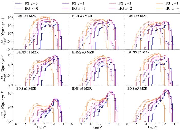
Figure 11 (Figure 12) shows the metallicity distribution of FGs and HGs we obtain if we adopt the MZR (FMR). The main difference between Figure 11 and 12 is that the distributions of both FGs and HGs extend to very low-metallicity tails in the case of the MZR, while they are truncated at in the case of the FMR.
For both the MZR (Figure 11) and FMR (Figure 12), the metallicity of the HG tends to be higher than the metallicity of the FG, because the average metallicity of the Universe increases as redshift decreases (Figure 4). The metallicity difference between HGs and FGs is particularly large for BBHs and BHNSs, which merger efficiency depends on metallicity, while it is negligible for BNSs.
Overall, BBHs tend to form in metal-poor galaxies and merge in metal-rich galaxies. This is particularly evident in the local Universe. In the case of BNSs, the peak of the metallicity distribution of FGs and HGs almost coincide.
3.3 Merger rate per galaxy
| BBH | FMR | ||||||||||
|---|---|---|---|---|---|---|---|---|---|---|---|
| MZR | |||||||||||
| A20a | |||||||||||
| BHNS | FMR | ||||||||||
| MZR | |||||||||||
| A20a | |||||||||||
| BNS | FMR | ||||||||||
| MZR | |||||||||||
| A20a | |||||||||||
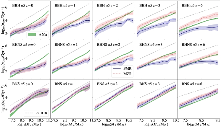
Figure 13 shows the merger rate per galaxy as function of the stellar mass. We compare our results to those of Artale et al. (2019) and Artale et al. (2020a), who adopt the eagle cosmological simulation to retrieve this information. The merger rate of BNSs strongly correlates with the stellar mass of the HG. The correlation slope (Table 2) is consistent with that obtained by Artale et al. (2020a) with cosmological simulations in the case of BNSs. To interpret this result, in Figure 13 we show the main sequence definition by B18, with an arbitrary normalisation. It is apparent that the correlation of with the stellar mass is mainly a consequence of the main sequence of star-forming galaxies.
Deviations from the main sequence are particularly evident in the case of BBHs and BHNSs. In fact, the merger rate per galaxy of BBHs and BHNSs also depends on the chosen metallicity relation. The merger rates per galaxy obtained with the MZR or FMR are almost identical in the local Universe, but become dramatically different at redshift , in terms of both slope and normalization. This happens because the differences between FMR and MZR increase with redshift (Figure 3). In fact, in the case of the FMR the formation of BBHs and BHNSs drops in galaxies with M⊙ at (Figure 8). As a result, the BBH merger rate per galaxy at has a much shallower trend with in the case of the FMR with respect to the MZR.
3.4 Role of passive galaxies
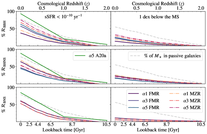
Figure 14 shows the percentage of compact object mergers in passive galaxies. Besides our definition of passive galaxies (Section 2.2.4), we also show the definition adopted by Artale et al. (2019), for comparison. According to the definition in Artale et al. (2019), passive galaxies are galaxies with specific SFR (sSFR) yr-1. Figure 14 shows that the contribution of passive galaxies to the merger rate increases as redshift decreases, for both definitions. This happens because the percentage of stellar mass stored in passive galaxies increases as we approach the local Universe.
With common envelope efficiency , which corresponds to longer delay times, the fraction of BBH mergers in passive galaxies is higher with respect to lower values of . The MZR predicts more BBH mergers in passive galaxies at fixed redshift with respect to the FMR, while the fraction of BNS mergers in passive galaxies does not depend on the chosen metallicity evolution.
4 Discussion
Here, we discuss some of the main assumptions we made in our model and their impact on our results. We will not consider the impact of binary population synthesis parameters, which we have already described in Santoliquido et al. (2021).
4.1 Constant versus variable GSMF
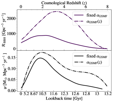
We assumed that the slope of the GSMF () is constant with redshift. Chruslinska & Nelemans (2019) pointed out that the slope of the low-mass end of the GSMF is weakly constrained. Although the low-mass galaxies are overall the most abundant, they are also the faintest and most difficult to observe, especially at high redshift. Table 1 in Chruslinska & Nelemans (2019) shows that the low-mass slope tends to steepen with redshift. In other words, in Equation 1 becomes more negative at increasing redshift (Figure 3 of Chruslinska & Nelemans 2019). Figure 15 shows the impact of the evolving low-mass slope of GSMF with redshift, , on the cosmic SFR density and on the merger rate density. For the latter, we show the case of BBHs, and MZR to maximise the impact of a higher fraction of metal-poor low-mass galaxies on the merger rate density. The cosmic SFRD varies at most by a factor of 4 at , resulting in a similar difference at in the merger rate density.
4.2 Main sequence of star forming and starburst galaxies
We assumed that the star-forming main sequence has no flattening at high masses, i.e. the linear relation is preserved at any value of stellar mass (equations 3 and 4). Chruslinska & Nelemans (2019) show that there can be two main variations with respect to this assumption. The first variation is referred to as moderate flattening. In this case the high-mass end of the main sequence is less steep than that of the low-mass end, and can also evolve with redshift becoming steeper with increasing (Speagle et al., 2014; Boogaard et al., 2018; Popesso et al., 2019). The second variation is called sharp flattening and the main sequence has an even sharper flattening at high masses (Tomczak et al., 2016). The resulting SFR is almost constant with increasing stellar mass (Figure 5 of Chruslinska & Nelemans 2019). We expect that the impact on our results of the moderate and sharp flattening of the main sequence of massive galaxies is lower with respect to changing the definition of the main sequence itself (i.e., considering both S14 and B18).
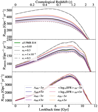
The distribution of star-forming galaxies at fixed mass (Equation 2) also relies on a number of parameters affected by observational uncertainties: , , , , and (see Table 1 and Section 2.2.2 for details). Figure 16 shows the impact of variations of these parameters on the merger rate density. The shift between starburst galaxies and main sequence (i.e., the definition of ) yields the largest differences () on the merger rate density of BBHs at . Overall, BNSs are less affected by these parameters than both BBHs and BHNSs, because they are less sensitive to metal-dependent star formation.
Recent papers (e.g. Caputi et al. 2017 and Bisigello et al. 2018) show that the percentage of starburst galaxies with respect to all star-forming galaxies might increase towards lower stellar masses and with redshift. This suggests that the contribution of starburst galaxies to the total cosmic SFR density is higher than our main assumption (Section 2.2.2). To see an example of the impact of this treatment of starburst galaxies on the SFRD, we refer to Chruślińska et al. (2021) (Figure 10). We will include the impact of this treatment of starburst galaxies in a follow-up study.
4.3 Metallicity relationships
The intrinsic scatter around both the MZR and the FMR is also uncertain, as well as the metallicity gradient within each galaxy, described by and , respectively (Section 2.2.3). We varied these parameters to assess their impact on the merger rate density, as shown in Figure 16. In the local Universe, the merger rate density of BBHs varies at most by % and % if we consider and 0.30 (0.30), respectively.
Previous works have proposed a third observational relation to describe the metallicity evolution of galaxies: the fundamental plane (Lara-López et al., 2010; Hunt et al., 2012; Hunt et al., 2016). Similarly to the FMR, the fundamental plane is independent of redshift, and relates metallicity, SFR and stellar mass. However, in the case of the fundamental plane these three quantities are linked in a two-dimensional plane. In this way, the value of the galaxy metallicity can be expressed as (Hunt et al., 2016):
| (6) |
As a result, at high mass there is no bending after the turn-over mass and thus the metallicity does not converge to an asymptotic value. At low mass instead, Equation 6 yields an even flatter trend with stellar mass at fixed SFR with respect to the FMR. Thanks to this behaviour, the fundamental plane yields a merger rate density evolution in between the FMR and the MZR.
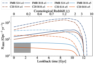
One last caveat concerns the calibration of metallicity in the adopted scaling relations. Empirical metallicity calibrations are one of the main sources of uncertainty in determining the metallicity of galaxies (Kewley & Ellison, 2008; Maiolino & Mannucci, 2019; Curti et al., 2020). In fact, different metallicity calibrations can give rise to different a normalisation (up to dex) and shape of the MZR (see, for example, Figure 4 of Chruslinska & Nelemans 2019). To assess the impact of a different metallicity calibration on our results, we evaluated the BBH merger rate density with the new definition of FMR given in Equation 5 of Curti et al. (2020, hereafter C20). The main difference between the FMR we adopted in our paper and the FMR derived by C20 is that the latter has a shallower slope for galaxies less massive than the turnover mass (); in other words, galaxies with M⊙ have higher metallicity at any SFR (lower panel of Figure 3 of C20). Figure 17 shows that the overall evolution of the BBH merger rate density with redshift is not heavily affected by this different metallicity calibration. On the other hand, the BBH merger rate density in the local Universe resulting from the FMR reported by C20 is a factor lower with respect to the FMR adopted in this work.
5 Conclusions
We developed the new code galaxyate, which estimates the merger rate density of binary compact objects (BCOs) and the properties of their host galaxies (HGs), based on observational scaling relations. With galaxyate, we can perform many realizations of the merger rate density and HG properties across the cosmic time, in order to bracket the main uncertainties springing from both BCO formation and galaxy evolution.
Here, we have adopted three BCO catalogues generated with the population-synthesis code mobse (Giacobbo & Mapelli, 2018b). In each catalogue, we vary the common-envelope efficiency parameter , 3 and 5. This parameter is one of the main sources of uncertainty among binary evolution processes (Santoliquido et al., 2021) and has a great impact on the delay time distribution of BCOs (Appendix B).
galaxyate first generates the formation galaxy (FG) of each BCO, i.e. the galaxy in which the progenitor stars of the BCO form. Each FG is described by its stellar mass, SFR and metallicity. We extract these properties from observational relations: the galaxy stellar mass function, the SFR distribution of star-forming and starburst galaxies, the mass–metallicity relation (MZR), and the fundamental metallicity relation (FMR). Given the large observational uncertainties, we explored the parameter space (Section 2.2) that mostly affects our results. For instance, we considered two galaxy main sequence definitions (S14 and B18). We also compared the metallicity evolution obtained with the MZR and FMR.
The HG (i.e., the galaxy in which the BCO merges) can be different from the FG for several reasons: the FG might have merged with other galaxies by the time the BCO reaches coalescence, or it might have evolved changing its mass, SFR and metallicity. We thus assign a HG to each BCO based on the conditional probability , i.e. the probability that the HG has mass and star formation rate , given the mass () and SFR () of the FG, and given the formation () and merger redshift () of the BCO (Section 2.4). Here, we calculate this probability in an empirical way by using the merger trees from the eagle cosmological simulation (Schaye et al., 2015; Qu et al., 2017).
We found that the merger rate density evolution with redshift changes dramatically depending on the choice of the star-forming galaxy main sequence, especially in the case of BBHs and BHNSs. The local merger rate density of BBHs and BHNSs is times higher if we assume the star-forming main sequence from S14 with respect to B18. This happens because the S14 main sequence predicts a significantly higher SFR density at high redshift with respect to B18 (Figure 2). BBHs and BHNSs are strongly affected by this difference, because their merger rate depends on metallicity and newly born stars at high redshift are preferentially metal-poor. In contrast, BNSs are marginally affected, because their merger rate does not depend on metallicity (Figure 6).
The choice of the metallicity evolution has an important effect on the slope of the merger rate density of BBHs and BHNSs. The slope of the merger rate density evolution of BBHs and BHNSs is steeper if we assume the MZR with respect to the FMR, because the latter predicts a shallower decrease of metallicity with redshift (Figure 6). In contrast, BNSs are not affected by the choice of the metallicity relation.
Also, we compared the merger rate density obtained with galaxyate (Section 2.3) with that obtained with cosmoate (Appendix A), which evaluates the merger rate density by assuming the average SFR density and metallicity evolution of the Universe, i.e. without information about the galaxies (Santoliquido et al., 2021). We found that the merger rate density evolution of BNSs obtained with cosmoate and galaxyate are in good agreement, while the BBH and BHNS merger rate densities evaluated with galaxyate are higher than those obtained with cosmoate, if we assume the fitting formulas from Madau & Fragos (2017) and a metallicity spread (Figure 6). The main reason is that the SFRD we obtain from the observational scaling relations supports a larger population of metal-poor stars with respect to the Madau & Fragos (2017) fitting formulas with . The differences between the BBH merger rate density obtained with galaxyate and cosmoate can be reconciled by assuming a larger metallicity spread in cosmoate.
The merger rate density of BNSs and BHNSs is within the 90% credible interval estimated by the LVK with GWTC-3 (Abbott et al., 2021b) for all considered assumptions, while the merger rate density of BBHs predicted by our models is higher than the LVK range. This discrepancy most likely originates from the interplay of several different sources of uncertainty. Firstly, we considered only the formation of BBHs from binary evolution, and neglected the dynamical formation channel, which is more effective for BBHs than for the other families of BCOs. Current models of binary evolution predict an extremely strong dependence of the BBH merger rate density on metallicity, while this dependence is quenched by most dynamical formation channels (e.g., Mapelli et al., 2022). It might be that the dependence of the BBH merger rate on metallicity is overestimated by current binary evolution models, or that most BBHs do not form via this channel. In a follow-up study, we will consider alternative formation channels for BBHs. Secondly, current models of binary evolution might overestimate the BBH merger rate because of our poor knowledge of several binary evolution processes, such as common envelope and the stability of Roche lobe (Marchant et al., 2021; Klencki et al., 2021; Gallegos-Garcia et al., 2021; Belczynski et al., 2022). Thirdly, the evolution of stellar metallicity across cosmic time is one of the most disputed aspects of galaxy evolution, because all the metallicity calibrations are affected by large (and sometimes systematic) uncertainties (Maiolino & Mannucci, 2019).
Overall, the HGs of BBHs and BHNSs are more massive than their FGs (both assuming the MZR and the FMR), because both BBHs and BHNSs tend to form in smaller metal-poor galaxies and to merge in larger metal-rich galaxies. In contrast, the FGs and HGs of BNSs are very similar to each other (Figures 7 and 8).
The mass distribution of HGs is affected by the delay time distribution. In our models, different values of the common-envelope efficiency result in different distributions of the delay time (Appendix B), with larger values of being associated with longer delay times. Figures 7 and 8 show that the contribution of high-mass galaxies increases with . In fact, with (longer delay times), the FG has more time to merge with other galaxies and form a more massive HG. On the other hand, for (shorter delay times), a large fraction of BBHs are hosted in low-mass galaxies.
In the high-redshift Universe () both the FGs and HGs of BCOs have a higher SFR than in the local Universe (Figures 9 and 10). Different values of have a mild impact on the shape of the SFR distribution of HGs. On the other hand, the FMR favours HGs with lower SFR with respect to the MZR in the case of BBHs at .
The FGs of BBHs and BHNSs tend to have a lower metallicity than their HGs, in the case of both MZR and FMR (Figures 11 and 12). However, the metallicity distributions of both FGs and HGs strongly depend on the choice of the metallicity relation. If we assume the MZR, the HGs and especially the FGs extend to lower metallicity at high redshift than in the local Universe. In contrast, the FMR predicts relatively high metallicities for both FGs and HGs and no significant trend with redshift.
We found a strong correlation between the BNS merger rate per galaxy () and the stellar mass of the HG (Figure 13). This correlation is less tight for BBHs and BHNSs, especially if we assume the FMR (Table 2).
Passive galaxies can host compact objects mergers (Figure 14). Their contribution increases as approaching the local Universe, regardless of the adopted passive galaxy definition. However, the percentage of mergers hosted in passive galaxies crucially depends on this definition. If all the galaxies with sSFR yr-1 are considered passive galaxies, we find that %, % and % of all BNS, BHNS and BBH mergers in the local Universe are associated with a passive galaxy, respectively. In contrast, if we define passive galaxies as those galaxies with SFR at least 1 dex below the star-forming main sequence, only %, % and % of all BNS, BHNS and BBH mergers in the local Universe are associated with a passive galaxy, respectively. Overall, BCOs have more chances to be hosted in passive galaxies if their delay time distribution is longer.
Acknowledgements
We thank Martyna Chruslinska, Irina Dvorkin, Stanislav Babak, Leslie K. Hunt, Filippo Mannucci, Giulia Rodighiero, Paolo Cassata and Francesco Sinigaglia for the insightful discussions. MM and FS acknowledge financial support from the European Research Council for the ERC Consolidator grant DEMOBLACK, under contract no. 770017. MCA acknowledges financial support from the Seal of Excellence @UNIPD 2020 programme under the ACROGAL project. FS thanks the Astroparticule et Cosmologie Laboratoire (APC) and the Institute d’Astrophysique de Paris (IAP) for hospitality during the preparation of this manuscript.
Data Availability
The data underlying this article will be shared on reasonable request to the corresponding authors. The latest public version of mobse can be downloaded from this repository. cosmoate is publicly available on GitLab at this link.
References
- Abbott et al. (2017a) Abbott R., et al., 2017a, Phys. Rev. Lett., 119, 161101
- Abbott et al. (2017b) Abbott R., et al., 2017b, Nature, 551, 85
- Abbott et al. (2017c) Abbott B. P., Abbott R., Abbott T. D., Acernese F., Ackley K., Adams C., Adams T., 2017c, ApJ, 848, L13
- Abbott et al. (2018) Abbott R., et al., 2018, Living Reviews in Relativity, 21, 3
- Abbott et al. (2021a) Abbott R., et al., 2021a, arXiv e-prints, p. arXiv:2111.03606
- Abbott et al. (2021b) Abbott R., et al., 2021b, arXiv e-prints, p. arXiv:2111.03634
- Ade et al. (2016) Ade P. A. R., et al., 2016, A&A, 594, A13
- Adhikari et al. (2020) Adhikari S., Fishbach M., Holz D. E., Wechsler R. H., Fang Z., 2020, ApJ, 905, 21
- Alexander et al. (2017) Alexander K. D., et al., 2017, ApJ, 848, L21
- Anders & Grevesse (1989) Anders E., Grevesse N., 1989, Geochimica Cosmochimica Acta, 53, 197
- Arcavi et al. (2017) Arcavi I., et al., 2017, ApJ, 848, L33
- Artale et al. (2019) Artale M. C., Mapelli M., Giacobbo N., Sabha N. B., Spera M., Santoliquido F., Bressan A., 2019, MNRAS, 487, 1675
- Artale et al. (2020a) Artale M. C., Mapelli M., Bouffanais Y., Giacobbo N., Pasquato M., Spera M., 2020a, MNRAS, 491, 3419
- Artale et al. (2020b) Artale M. C., Bouffanais Y., Mapelli M., Giacobbo N., Sabha N. B., Santoliquido F., Pasquato M., Spera M., 2020b, MNRAS, 495, 1841
- Ashkar et al. (2021a) Ashkar H., et al., 2021a, arXiv e-prints, p. arXiv:2108.04654
- Ashkar et al. (2021b) Ashkar H., et al., 2021b, J. Cosmology Astropart. Phys., 2021, 045
- Asplund et al. (2009) Asplund M., Grevesse N., Sauval A. J., Scott P., 2009, ARA&A, 47, 481
- Baibhav et al. (2019) Baibhav V., Berti E., Gerosa D., Mapelli M., Giacobbo N., Bouffanais Y., Di Carlo U. N., 2019, Phys. Rev. D, 100, 064060
- Belczynski et al. (2006) Belczynski K., Perna R., Bulik T., Kalogera V., Ivanova N., Lamb D. Q., 2006, ApJ, 648, 1110
- Belczynski et al. (2016) Belczynski K., et al., 2016, A&A, 594, A97
- Belczynski et al. (2022) Belczynski K., et al., 2022, ApJ, 925, 69
- Béthermin et al. (2012) Béthermin M., et al., 2012, ApJ, 757, L23
- Bisigello et al. (2018) Bisigello L., Caputi K. I., Grogin N., Koekemoer A., 2018, A&A, 609, A82
- Boco et al. (2019) Boco L., Lapi A., Goswami S., Perrotta F., Baccigalupi C., Danese L., 2019, ApJ, 881, 157
- Boco et al. (2021) Boco L., Lapi A., Chruslinska M., Donevski D., Sicilia A., Danese L., 2021, ApJ, 907, 110
- Boogaard et al. (2018) Boogaard L. A., et al., 2018, A&A, 619, A27
- Caffau et al. (2011) Caffau E., Ludwig H. G., Steffen M., Freytag B., Bonifacio P., 2011, Sol. Phys., 268, 255
- Caputi et al. (2017) Caputi K. I., et al., 2017, ApJ, 849, 45
- Casey et al. (2018) Casey C. M., et al., 2018, ApJ, 862, 77
- Chabrier (2003) Chabrier G., 2003, PASP, 115, 763
- Chen et al. (2022) Chen X., Wang J., Kong X., 2022, ApJ, 933, 39
- Chornock et al. (2017) Chornock R., et al., 2017, ApJ, 848, L19
- Chruslinska & Nelemans (2019) Chruslinska M., Nelemans G., 2019, MNRAS, 488, 5300
- Chruślińska et al. (2020) Chruślińska M., Jeřábková T., Nelemans G., Yan Z., 2020, A&A, 636, A10
- Chruślińska et al. (2021) Chruślińska M., Nelemans G., Boco L., Lapi A., 2021, MNRAS, 508, 4994
- Chu et al. (2021) Chu Q., Yu S., Lu Y., 2021, MNRAS,
- Cigarrán Díaz & Mukherjee (2022) Cigarrán Díaz C., Mukherjee S., 2022, MNRAS, 511, 2782
- Claeys et al. (2014) Claeys J. S. W., Pols O. R., Izzard R. G., Vink J., Verbunt F. W. M., 2014, A&A, 563, A83
- Conselice et al. (2016) Conselice C. J., Wilkinson A., Duncan K., Mortlock A., 2016, ApJ, 830, 83
- Coulter et al. (2017) Coulter D. A., et al., 2017, Science, 358, 1556
- Cowperthwaite et al. (2017) Cowperthwaite P. S., et al., 2017, ApJ, 848, L17
- Curti et al. (2020) Curti M., Mannucci F., Cresci G., Maiolino R., 2020, MNRAS, 491, 944
- Curti et al. (2022) Curti M., et al., 2022, arXiv e-prints, p. arXiv:2207.12375
- Daddi et al. (2007) Daddi E., et al., 2007, ApJ, 670, 156
- Dominik et al. (2012) Dominik M., Belczynski K., Fryer C., Holz D. E., Berti E., Bulik T., Mandel I., O’Shaughnessy R., 2012, ApJ, 759, 52
- Dominik et al. (2013) Dominik M., Belczynski K., Fryer C., Holz D. E., Berti E., Bulik T., Mandel I., O’Shaughnessy R., 2013, ApJ, 779, 72
- Donnari et al. (2019) Donnari M., et al., 2019, MNRAS, 485, 4817
- Donnari et al. (2021) Donnari M., Pillepich A., Nelson D., Marinacci F., Vogelsberger M., Hernquist L., 2021, MNRAS, 506, 4760
- Ducoin et al. (2020) Ducoin J. G., Corre D., Leroy N., Le Floch E., 2020, MNRAS, 492, 4768
- Ebrová et al. (2020) Ebrová I., Bílek M., Yıldız M. K., Eliášek J., 2020, A&A, 634, A73
- Efstathiou (2000) Efstathiou G., 2000, MNRAS, 317, 697
- Elbert et al. (2018) Elbert O. D., Bullock J. S., Kaplinghat M., 2018, MNRAS, 473, 1186
- Fishbach et al. (2019) Fishbach M., et al., 2019, ApJ, 871, L13
- Fryer et al. (2012) Fryer C. L., Belczynski K., Wiktorowicz G., Dominik M., Kalogera V., Holz D. E., 2012, ApJ, 749, 91
- Furlong et al. (2015) Furlong M., et al., 2015, MNRAS, 450, 4486
- Gallegos-Garcia et al. (2021) Gallegos-Garcia M., Berry C. P. L., Marchant P., Kalogera V., 2021, ApJ, 922, 110
- Genzel et al. (2015) Genzel R., et al., 2015, ApJ, 800, 20
- Giacobbo & Mapelli (2018a) Giacobbo N., Mapelli M., 2018a, MNRAS, 480, 2011
- Giacobbo & Mapelli (2018b) Giacobbo N., Mapelli M., 2018b, MNRAS, 480, 2011
- Giacobbo & Mapelli (2019) Giacobbo N., Mapelli M., 2019, MNRAS, 482, 2234
- Giacobbo & Mapelli (2020) Giacobbo N., Mapelli M., 2020, ApJ, 891, 141
- Goldstein et al. (2017) Goldstein A., et al., 2017, ApJ, 848, L14
- Gray et al. (2020) Gray R., et al., 2020, Phys. Rev. D, 101, 122001
- Grevesse & Sauval (1998) Grevesse N., Sauval A. J., 1998, Space Sci. Rev., 85, 161
- Gruppioni et al. (2020) Gruppioni C., et al., 2020, A&A, 643, A8
- Hobbs et al. (2005) Hobbs G., Lorimer D. R., Lyne A. G., Kramer M., 2005, MNRAS, 360, 974
- Hopkins et al. (2012) Hopkins P. F., Quataert E., Murray N., 2012, MNRAS, 421, 3522
- Hunt et al. (2012) Hunt L., et al., 2012, MNRAS, 427, 906
- Hunt et al. (2016) Hunt L., Dayal P., Magrini L., Ferrara A., 2016, MNRAS, 463, 2020
- Hurley et al. (2000) Hurley J. R., Pols O. R., Tout C. A., 2000, MNRAS, 315, 543
- Hurley et al. (2002) Hurley J. R., Tout C. A., Pols O. R., 2002, MNRAS, 329, 897
- Ilbert et al. (2013) Ilbert O., et al., 2013, A&A, 556, A55
- Ilbert et al. (2015) Ilbert O., et al., 2015, A&A, 579, A2
- Im et al. (2017) Im M., et al., 2017, ApJ, 849, L16
- Inayoshi et al. (2017) Inayoshi K., Hirai R., Kinugawa T., Hotokezaka K., 2017, MNRAS, 468, 5020
- Jin et al. (2021) Jin S.-J., Wang L.-F., Wu P.-J., Zhang J.-F., Zhang X., 2021, Phys. Rev. D, 104, 103507
- Kalogera et al. (2019) Kalogera V., et al., 2019, BAAS, 51, 242
- Kalogera et al. (2021) Kalogera V., et al., 2021, arXiv e-prints, p. arXiv:2111.06990
- Kewley & Ellison (2008) Kewley L. J., Ellison S. L., 2008, ApJ, 681, 1183
- Kilpatrick et al. (2022) Kilpatrick C. D., et al., 2022, ApJ, 926, 49
- Klencki et al. (2018) Klencki J., Moe M., Gladysz W., Chruslinska M., Holz D. E., Belczynski K., 2018, A&A, 619, A77
- Klencki et al. (2021) Klencki J., Nelemans G., Istrate A. G., Chruslinska M., 2021, A&A, 645, A54
- Knebe et al. (2011) Knebe A., et al., 2011, MNRAS, 415, 2293
- Kopparapu et al. (2008) Kopparapu R. K., Hanna C., Kalogera V., O’Shaughnessy R., González G., Brady P. R., Fairhurst S., 2008, ApJ, 675, 1459
- Kovlakas et al. (2021) Kovlakas K., et al., 2021, MNRAS, 506, 1896
- Kroupa (2001) Kroupa P., 2001, MNRAS, 322, 231
- Lamberts et al. (2016) Lamberts A., Garrison-Kimmel S., Clausen D. R., Hopkins P. F., 2016, MNRAS, 463, L31
- Lapi et al. (2020) Lapi A., Pantoni L., Boco L., Danese L., 2020, ApJ, 897, 81
- Lara-López et al. (2010) Lara-López M. A., et al., 2010, A&A, 521, L53
- Leandro et al. (2022) Leandro H., Marra V., Sturani R., 2022, Phys. Rev. D, 105, 023523
- Leja et al. (2021) Leja J., et al., 2021, arXiv e-prints, p. arXiv:2110.04314
- Levan et al. (2017) Levan A. J., et al., 2017, ApJ, 848, L28
- Libanore et al. (2021) Libanore S., et al., 2021, J. Cosmology Astropart. Phys., 2021, 035
- Libanore et al. (2022) Libanore S., Artale M. C., Karagiannis D., Liguori M., Bartolo N., Bouffanais Y., Mapelli M., Matarrese S., 2022, J. Cosmology Astropart. Phys., 2022, 003
- Liu & Bromm (2021) Liu B., Bromm V., 2021, MNRAS, 506, 5451
- Mac Low & Ferrara (1999) Mac Low M.-M., Ferrara A., 1999, ApJ, 513, 142
- Madau & Dickinson (2014) Madau P., Dickinson M., 2014, ARA&A, 52, 415
- Madau & Fragos (2017) Madau P., Fragos T., 2017, ApJ, 840, 39
- Maggiore et al. (2020) Maggiore M., et al., 2020, J. Cosmology Astropart. Phys., 2020, 050
- Magnelli et al. (2012) Magnelli B., et al., 2012, A&A, 539, A155
- Maiolino & Mannucci (2019) Maiolino R., Mannucci F., 2019, A&ARv, 27, 3
- Maiolino et al. (2008) Maiolino R., et al., 2008, A&A, 488, 463
- Mandhai et al. (2022) Mandhai S., Lamb G. P., Tanvir N. R., Bray J., Nixon C. J., Eyles-Ferris R. A. J., Levan A. J., Gompertz B. P., 2022, MNRAS, 514, 2716
- Mannucci et al. (2009) Mannucci F., et al., 2009, MNRAS, 398, 1915
- Mannucci et al. (2010) Mannucci F., Cresci G., Maiolino R., Marconi A., Gnerucci A., 2010, MNRAS, 408, 2115
- Mannucci et al. (2011) Mannucci F., Salvaterra R., Campisi M. A., 2011, MNRAS, 414, 1263
- Mapelli et al. (2017) Mapelli M., Giacobbo N., Ripamonti E., Spera M., 2017, MNRAS, 472, 2422
- Mapelli et al. (2018a) Mapelli M., Giacobbo N., Toffano M., Ripamonti E., Bressan A., Spera M., Branchesi M., 2018a, MNRAS, 481, 5324
- Mapelli et al. (2018b) Mapelli M., Giacobbo N., Toffano M., Ripamonti E., Bressan A., Spera M., Branchesi M., 2018b, MNRAS, 481, 5324
- Mapelli et al. (2019) Mapelli M., Giacobbo N., Santoliquido F., Artale M. C., 2019, MNRAS, 487, 2
- Mapelli et al. (2020) Mapelli M., Spera M., Montanari E., Limongi M., Chieffi A., Giacobbo N., Bressan A., Bouffanais Y., 2020, ApJ, 888, 76
- Mapelli et al. (2022) Mapelli M., Bouffanais Y., Santoliquido F., Arca Sedda M., Artale M. C., 2022, MNRAS, 511, 5797
- Marchant et al. (2021) Marchant P., Pappas K. M. W., Gallegos-Garcia M., Berry C. P. L., Taam R. E., Kalogera V., Podsiadlowski P., 2021, A&A, 650, A107
- Margutti et al. (2017) Margutti R., et al., 2017, ApJ, 848, L20
- McAlpine et al. (2016) McAlpine S., et al., 2016, Astronomy and Computing, 15, 72
- McCarthy et al. (2020) McCarthy K. S., Zheng Z., Ramirez-Ruiz E., 2020, MNRAS, 499, 5220
- McLeod et al. (2021) McLeod D. J., McLure R. J., Dunlop J. S., Cullen F., Carnall A. C., Duncan K., 2021, MNRAS, 503, 4413
- Moffett et al. (2016) Moffett A. J., et al., 2016, MNRAS, 457, 1308
- Mukherjee & Moradinezhad Dizgah (2021) Mukherjee S., Moradinezhad Dizgah A., 2021, arXiv e-prints, p. arXiv:2111.13166
- Mukherjee et al. (2021) Mukherjee S., Wandelt B. D., Nissanke S. M., Silvestri A., 2021, Phys. Rev. D, 103, 043520
- Muldrew et al. (2011) Muldrew S. I., Pearce F. R., Power C., 2011, MNRAS, 410, 2617
- Neijssel et al. (2019) Neijssel C. J., et al., 2019, MNRAS, 490, 3740
- Ng et al. (2021) Ng K. K. Y., Vitale S., Farr W. M., Rodriguez C. L., 2021, ApJ, 913, L5
- Nicholl et al. (2017) Nicholl M., et al., 2017, ApJ, 848, L18
- O’Shaughnessy et al. (2010) O’Shaughnessy R., Kalogera V., Belczynski K., 2010, ApJ, 716, 615
- O’Shaughnessy et al. (2017) O’Shaughnessy R., Bellovary J. M., Brooks A., Shen S., Governato F., Christensen C. R., 2017, MNRAS, 464, 2831
- Pantoni et al. (2019) Pantoni L., Lapi A., Massardi M., Goswami S., Danese L., 2019, ApJ, 880, 129
- Peeples et al. (2014) Peeples M. S., Werk J. K., Tumlinson J., Oppenheimer B. D., Prochaska J. X., Katz N., Weinberg D. H., 2014, ApJ, 786, 54
- Perna & Belczynski (2002) Perna R., Belczynski K., 2002, ApJ, 570, 252
- Perna et al. (2022) Perna R., Artale M. C., Wang Y.-H., Mapelli M., Lazzati D., Sgalletta C., Santoliquido F., 2022, MNRAS, 512, 2654
- Pian et al. (2017) Pian E., et al., 2017, Nature, 551, 67
- Popesso et al. (2019) Popesso P., et al., 2019, MNRAS, 483, 3213
- Popesso et al. (2022) Popesso P., et al., 2022, arXiv e-prints, p. arXiv:2203.10487
- Pozzetti et al. (2010) Pozzetti L., et al., 2010, A&A, 523, A13
- Punturo et al. (2010) Punturo M., et al., 2010, Classical and Quantum Gravity, 27, 194002
- Qu et al. (2017) Qu Y., et al., 2017, MNRAS, 464, 1659
- Reitze et al. (2019) Reitze D., et al., 2019, in Bulletin of the American Astronomical Society. p. 35 (arXiv:1907.04833)
- Renzini & Peng (2015) Renzini A., Peng Y.-j., 2015, ApJ, 801, L29
- Rodighiero et al. (2011) Rodighiero G., et al., 2011, ApJ, 739, L40
- Rodighiero et al. (2015) Rodighiero G., et al., 2015, ApJ, 800, L10
- Rose et al. (2021) Rose J. C., Torrey P., Lee K. H., Bartos I., 2021, ApJ, 909, 207
- Safarzadeh & Berger (2019) Safarzadeh M., Berger E., 2019, ApJ, 878, L12
- Safarzadeh et al. (2019) Safarzadeh M., Berger E., Leja J., Speagle J. S., 2019, ApJ, 878, L14
- Sana et al. (2012) Sana H., et al., 2012, Science, 337, 444
- Sánchez-Menguiano et al. (2016) Sánchez-Menguiano L., et al., 2016, A&A, 587, A70
- Sánchez et al. (2014) Sánchez S. F., et al., 2014, A&A, 563, A49
- Sanders et al. (2020) Sanders R. L., et al., 2020, MNRAS, 491, 1427
- Santini et al. (2021) Santini P., et al., 2021, A&A, 652, A30
- Santoliquido et al. (2020) Santoliquido F., Mapelli M., Bouffanais Y., Giacobbo N., Di Carlo U. N., Rastello S., Artale M. C., Ballone A., 2020, ApJ, 898, 152
- Santoliquido et al. (2021) Santoliquido F., Mapelli M., Giacobbo N., Bouffanais Y., Artale M. C., 2021, MNRAS, 502, 4877
- Sargent et al. (2012) Sargent M. T., Béthermin M., Daddi E., Elbaz D., 2012, ApJ, 747, L31
- Savchenko et al. (2017) Savchenko V., et al., 2017, ApJ, 848, L15
- Schaye et al. (2015) Schaye J., et al., 2015, MNRAS, 446, 521
- Schechter (1976) Schechter P., 1976, ApJ, 203, 297
- Schneider et al. (2017) Schneider R., Graziani L., Marassi S., Spera M., Mapelli M., Alparone M., Bennassuti M. d., 2017, MNRAS, 471, L105
- Schreiber et al. (2015) Schreiber C., et al., 2015, A&A, 575, A74
- Soares-Santos et al. (2017) Soares-Santos M., et al., 2017, ApJ, 848, L16
- Speagle et al. (2014) Speagle J. S., Steinhardt C. L., Capak P. L., Silverman J. D., 2014, ApJS, 214, 15
- Spera & Mapelli (2017) Spera M., Mapelli M., 2017, MNRAS, 470, 4739
- Spera et al. (2019) Spera M., Mapelli M., Giacobbo N., Trani A. A., Bressan A., Costa G., 2019, MNRAS, 485, 889
- Stachie et al. (2020) Stachie C., Coughlin M. W., Christensen N., Muthukrishna D., 2020, MNRAS, 497, 1320
- Tanikawa et al. (2021) Tanikawa A., Susa H., Yoshida T., Trani A. A., Kinugawa T., 2021, ApJ, 910, 30
- Toffano et al. (2019) Toffano M., Mapelli M., Giacobbo N., Artale M. C., Ghirlanda G., 2019, MNRAS, 489, 4622
- Tomczak et al. (2016) Tomczak A. R., et al., 2016, ApJ, 817, 118
- Tremonti et al. (2004) Tremonti C. A., et al., 2004, ApJ, 613, 898
- Vijaykumar et al. (2020) Vijaykumar A., Saketh M. V. S., Kumar S., Ajith P., Choudhury T. R., 2020, arXiv e-prints, p. arXiv:2005.01111
- Villante et al. (2014) Villante F. L., Serenelli A. M., Delahaye F., Pinsonneault M. H., 2014, ApJ, 787, 13
- Webbink (1984) Webbink R. F., 1984, ApJ, 277, 355
- Zahid et al. (2014) Zahid H. J., Dima G. I., Kudritzki R.-P., Kewley L. J., Geller M. J., Hwang H. S., Silverman J. D., Kashino D., 2014, ApJ, 791, 130
Appendix A cosmoate
cosmoate estimates the merger rate density based on the average SFR density and metallicity evolution of the Universe, i.e. without considering individual galaxies (Santoliquido et al., 2020; Santoliquido et al., 2021). cosmoate interfaces catalogues of simulated BCOs with an observation-based metallicity-dependent SFR density evolution of the Universe SFRD. Namely, cosmoate estimates the merger rate density as
| (7) |
where
| (8) |
In the above equation, is the Hubble constant, and are the matter and energy density, respectively. We adopt the values in Ade et al. (2016). The term is given by:
| (9) |
where is the total simulated initial stellar mass, and is the rate of BCOs forming from stars with initial metallicity at redshift and merging at , extracted from our population-synthesis catalogues. In cosmoate, is given by
| (10) |
where is the cosmic SFR density at formation redshift from Madau & Fragos (2017), and is the log-normal distribution of metallicities at fixed formation redshift , with average and spread . Here, we consider two definitions of . Equation 4 of Santoliquido et al. (2020), hereafter model S20:
| (11) |
where and ; and Equation 6 of Madau & Fragos (2017), hereafter MF17, that is:
| (12) |
For these models, we considered two different values of the dispersion: for S20 and for MF17. In Figure 6 we also explore 0.6 and 0.7 for MF17.
Appendix B Delay time distributions and merger efficiency
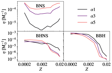
The merger efficiency and delay time distribution of BBHs strongly depend on metallicity and . Figure 18 show the merger efficiency , defined as:
| (13) |
where is the binary fraction (Sana et al., 2012), and is a correction factor taking into account that we simulated only stars with mass M⊙ with mobse. Thus, assuming a Kroupa IMF (Kroupa, 2001), .
Figure 18 shows that the merger efficiency decreases by four orders of magnitude if we vary to . This strong dependence of on has been already widely described in the literature and is common to very different population-synthesis codes (e.g. Dominik et al. 2012; Giacobbo & Mapelli 2018b; Klencki et al. 2018; Neijssel et al. 2019; Spera et al. 2019). It is a consequence of stellar winds: metal-poor stars retain larger masses during their lives and grow larger radii than metal-rich ones. This enhances their chances to undergo mass transfer with companion stars and produce tight BBHs.
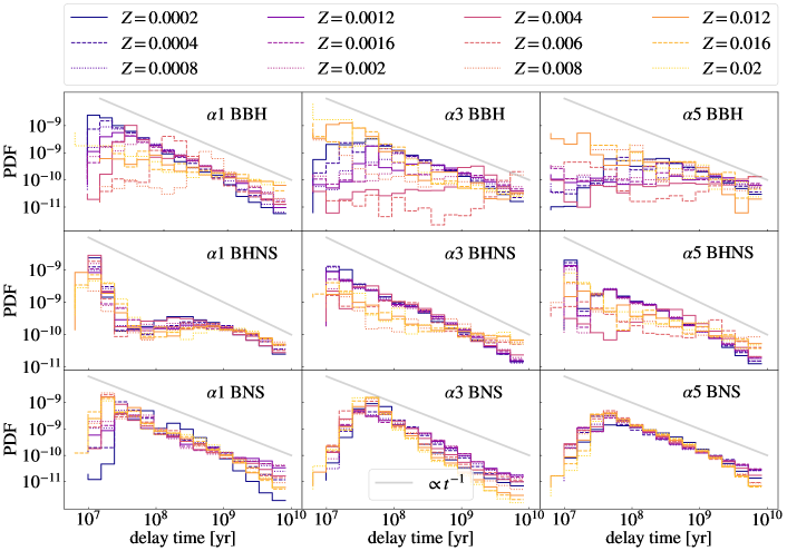
The merger efficiency of BNSs varies much less with but is heavily affected by . The parameter also shapes the distribution of delay times. Figure 19 shows that if the delay time distribution peaks at shorter delay times than for larger values of . Smaller values of correspond to shorter delay times, because a small value of implies a more effective shrinking of the progenitor binary during common envelope. Hence, binary compact objects tend to form with shorter orbital separation if we assume a lower value of . Also, Figure 19 shows that for long delay times.
Appendix C Impact of the comoving volume on the merger rate
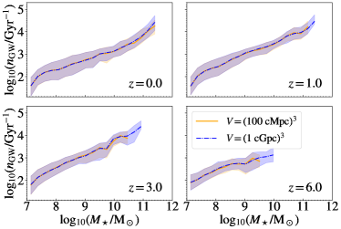
We assumed a comoving volume to obtain the results presented in the main text. This choice is a compromise between the need to sample a large volume and the computational cost: it takes and CPU hours to simulate a volume and , respectively. Figure 20 compares the case in which we assume and for one test case (with , FMR and B18). We find statistically no differences between the two volumes at redshift , while at higher redshift considering a large volume allows us to include more massive galaxies. Overall, we find no differences in the mass range we considered in this study, and our main results can be easily extrapolated to larger galaxy masses.
Appendix D Impact of the minimum galaxy mass on the merger rate
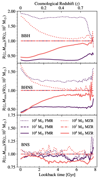
In our main text, we adopted a value M⊙ for the minimum galaxy stellar mass. In the local Universe, we see galaxies with mass lower than M⊙, but it is not clear if we can extrapolate the main scaling relations (GSMF, SFR, MZR and FMR) down to such small masses. Actually, there is a mild evidence that the lowest mass star forming galaxies deviate from the main observational scaling relations (e.g., Hunt et al., 2012).
Figure 21 shows the impact of two other choices of the minimum galaxy stellar masses, namely , and M⊙. In particular, we show the ratio of the merger rate density we obtain by varying the minimum galaxy stellar mass to the merger rate density we obtain for the fiducial value M⊙.
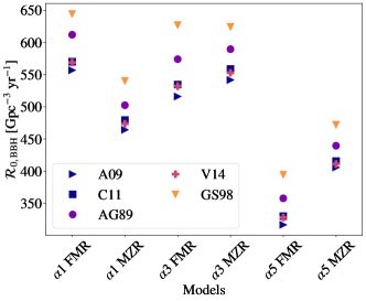
A lower (higher) value of implies a higher (lower) merger rate density for both BBHs and BHNSs, because of their dependence on the metallicity of the progenitor stars. We find a maximum difference of a factor of two between the BBH merger rate density with M⊙ and M⊙. This difference is nearly constant across redshift for the FMR, while it becomes smaller at high redshift for the MZR. In contrast, BNSs are not affected by the choice of .
Appendix E Impact of the solar metallicity on the merger rate density
| Reference | |||
|---|---|---|---|
| Asplund et al. (2009) | A09 | 0.0134 | 8.69 |
| Caffau et al. (2011) | C11 | 0.0153 | 8.76 |
| Anders & Grevesse (1989) | AG89 | 0.017 | 8.83 |
| Villante et al. (2014) | V14 | 0.019 | 8.85 |
| Grevesse & Sauval (1998) | GS98 | 0.0201 | 8.93 |
Both the MZR and FMR are expressed in terms of the relative abundance of oxygen and hydrogen . In order to convert this quantity to the mass fraction of all elements heavier than helium , we assumed, as commonly done in literature (e.g. Maiolino & Mannucci, 2019), that the latter scales linearly with the measured . In other words, we assumed that maintains the solar abundance ratio, as expressed by the following equation:
| (14) |
Figure 22 shows the impact of different definitions of the solar metallicity (Table 3) on the merger rate density of BBHs, which are the most affected by metallicity variations among BCOs. We show only the local merger rate density since changing the definition of the solar metallicity only affects the normalisation of the merger rate density.