Graph-theoretic approach to Bell experiments with low detection efficiency
Abstract
Bell inequality tests where the detection efficiency is below a certain threshold can be simulated with local hidden-variable models. Here, we introduce a method to identify Bell tests requiring low and relatively low dimension of the local quantum systems. The method has two steps. First, we show a family of bipartite Bell inequalities for which, for correlations produced by maximally entangled states, can be upper bounded by a function of some invariants of graphs, and use it to identify correlations that require small . We present examples in which, for maximally entangled states, for , for , and for . We also show evidence that the upper bound for can be lowered down to for and present a method to make the upper bound of arbitrarily small by increasing the dimension and the number of settings. All these upper bounds for are valid (as it is the case in the literature) assuming no noise. The second step is based on the observation that, using the initial state and measurement settings identified in the first step, we can construct Bell inequalities with smaller and better noise robustness. For that, we use a modified version of Gilbert’s algorithm that takes advantage of the automorphisms of the graphs used in the first step. We illustrate its power by explicitly developing an example in which is lower and the required visibility is lower than the upper bounds obtained in the first step. The tools presented here may allow for developing high-dimensional loophole-free Bell tests and loophole-free Bell nonlocality over long distances.
1 Introduction
Bell nonlocality [1, 2], that is, the violation of inequalities satisfied by any local hidden-variable (LHV) model, called Bell inequalities, is one of the most fascinating features of quantum mechanics and a crucial mean to accomplish tasks that are impossible with classical resources.
The detection efficiency in an experimental test of a Bell inequality is the ratio between the number of systems detected by one party and the number of pairs emitted by the source. depends not only on the efficiency of the detectors, but also on all the losses occurring during the distribution of the state. Pearle [3] and Wigner [4] noticed that experimental correlations in Bell inequality tests where the detection efficiency is below a certain threshold can be simulated by LHV models. Therefore, if is not high enough, the quantum advantage in many Bell inequality-based protocols (e.g., for randomness expansion [5, 6, 8, 7] and secure key distribution [9, 10, 11, 12, 13]) vanishes. Avoiding this so-called “detection loophole” requires surpassing . However, depends on the quantum correlations (i.e., the state prepared and the measurements performed) and the targeted Bell inequality.
In this work, we identify quantum correlations and Bell inequalities requiring the smallest reported, to our knowledge, in the literature for symmetric Bell tests (i.e., those in which all detectors have the same detection efficiency). The correlations are produced by maximally entangled states of experimentally accessible dimensions (e.g., ) and two-outcome measurements. In addition, we describe a method that provides arbitrarily small but requires higher dimensions.
The importance of these results lies on the fact that they pave the way to extend the groundbreaking loophole-free Bell tests performed on quantum systems of dimension (i.e., qubits) and distances between and m [17, 14, 15, 16] to quantum systems of higher dimensions and longer distances.
1.1 Structure of the paper
In Sec. 2, we collect the smallest values of reported in the literature and explain how they have been obtained. We also recall a standard form of expressing Bell functionals that will be used in several places.
Finding states, measurements, and Bell inequalities leading to small values of is difficult. One of the reasons is that, as we will see, these values occur for Bell inequalities with many settings for which computing the local bound is, in general, intractable [18]. Another reason is the difficulty of, given a Bell inequality, finding the state and measurements producing maximal quantum violations.
In Sec. 3, we introduce a method that overcomes both problems, as it connects the local bound of a family of bipartite Bell inequalities to the independence number of a graph, and quantum realizations that maximally violate the Bell inequalities to orthogonal representations of the graph. This allows us to identify examples of quantum correlations and Bell inequalities with unprecedentedly low .
In Sec. 4, we present a method based on graph theory to obtain explicit states and measurements making arbitrarily close to zero.
There are, however, two problems that make the examples obtained up to that point not useful in practice. One is that, in some cases, they require too many settings. In Sec. 5, we present a method for searching for examples with low and smaller number of settings.
The other problem is that, by construction, the quantum violations of the graph-based Bell inequalities are very sensitive to noise. In Sec. 6, we explain why and present a method to address this problem. The method applies to any of the (highly-symmetric) examples identified with the techniques in Sec. 3 and produces a Bell inequality for the same correlations (i.e., the same state and measurements) with smaller and higher resistance to noise.
Finally, in Sec. 7, we discuss how the different methods presented in this work can help us to design loophole-free Bell tests between high-dimensional quantum systems and achieve loophole-free Bell nonlocality over longer distances.
2 Previous works
2.1 Existing values of
For symmetric Bell tests and perfect visibility (as defined later), using maximally entangled states [19] for the simplest Bell inequality (the one with two dichotomic settings per party): the Clauser-Horne-Shimony-Holt (CHSH) inequality [20]. Eberhard [21] noticed that can be further reduced using nonmaximally entangled states and, in particular, that it can be lowered down to for the Clauser-Horne (CH) inequality [22].
For Bell inequalities with four settings and maximally entangled states, is not better than for CHSH (with one exception that allows a slightly lower value; ) [23, 24].
Although loophole-free Bell tests [17, 14, 15, 16] have proven that it is possible to produce correlations between local quantum systems of dimension that do not admit LHV models, the value of required in these experiments ( due to the noise) prevents real-life applications and, in particular, applications outside laboratories with well controlled losses, or involving longer distances (e.g., km). It is in this sense that the requirement of (without noise, with noise) acts as a bottleneck that blocks many real-life applications.
Massar [25] discovered that high-dimensional systems can tolerate a detection efficiency that decreases with the dimension of the local quantum system. However, he only found an improvement over the qubit case for . Vértesi, Pironio, and Brunner [26] lowered down to for maximally entangled states and to for nonmaximally entangled states using .
Márton, Bene, and Vértesi [27] have studied the case of copies of the two-qubit maximally entangled state and local Pauli measurements which act in the corresponding qubit subsystems. They obtained the following upper bounds for : for (which is equivalent to ), for (which is equivalent to ), and for (which is equivalent to ). More recently, Miklin et al. have reported a method that allows us to reduce down to for [28].
In this article, we focus on the case of two parties and symmetric detection efficiency, since we see it as the closest one for realistic applications. However, it should be mentioned that another way of obtaining low is by considering Bell experiments involving spatially separated parties [29, 30, 31]. Still, the difficulty for preparing and distributing the required states makes the resulting values unpractical for actual applications. In addition, it should also be pointed out that can be reduced for some detectors at the expense of requiring for other detectors [32, 33, 34, 35].
2.2 Calculating
Here, we summarize the different ways for calculating that can be found in the literature for the case that the propagation losses and detection inefficiencies are the same for all the detectors. For a more detailed discussion, see Ref. [36].
In an ideal Bell test, every run would end up with the two particles emitted by the source being detected, one at one party’s site and the other at the other party’s. However, in a real Bell test this may not be the case. As pointed out before, reasons for that are the existence of propagation losses and the imperfection of the detectors. Consequently, a detection at one site may not be accompanied with a detection at the other site and also, in some runs, both particles may be undetected.
In some cases, in addition to the local losses and imperfect detectors, the particles are not emitted at well-known times, then the number of emitted pairs, and thus the number of runs of the Bell test, will be unknown.
Below we summarize how can be calculated in each case.
Case I. The number of runs is known. This is the case in event-ready experiments [37, 17, 16] and in the proposals [38, 39, 40, 41] and experiments [42] with heralded detection.
Case I. Strategy I. We can associate the no-detection with a new outcome of the measurement and find a new Bell inequality with the same number of settings but one more outcome per setting than in the original Bell inequality. Then, the experiment will be free of the detection loophole as soon as the new inequality is violated. The problem is that finding this new Bell inequality may be difficult.
For example, if we add a new outcome to all the measurements in the Bell scenario (i.e., the one with parties, settings per party, and outcomes), then we end up in the Bell scenario. Then, the number of deterministic LHV assignments changes from to . Meanwhile, the dimension of the LHV assignments changes from to . To make clear the difficulties that finding such Bell inequalities involve, notice that, so far, we do not know the Bell inequalities for any Bell scenario.
Case I. Strategy II. We can associate the no-detection with one of the outcomes of each measurement and use the original Bell inequality. Then, the experiment will be loophole-free as soon as the original Bell inequality is violated.
To obtain in this case, we can act as follows. In an ideal Bell test in which we could achieve the maximum quantum value of a Bell expression whose bound for LHV models is , and in which the experimental detection efficiency is , the experimental value of would be
| (1) |
where is the value of resulting of what the parties output when Alice has detected the particle but not Bob (and similarly ), and is the value that the parties output when both Alice and Bob have not detected the particles. Usually, the outputs are chosen such that . The critical detection efficiency using this strategy is
| (2) |
This is the strategy used to obtain all the values previously reported except the ones in [21, 26]. This will also be the strategy used in this paper.
Case II. The number of runs is not known. This is the case in existing photonic Bell tests with high detection efficiency [43, 44, 45, 46, 47, 48, 49, 50, 51, 52, 53, 54].
Case II. Strategy III. This strategy works for the CH Bell inequality [22], for inequalities that can be written in terms of the CH functional [26], and for some Bell inequalities that can be rewritten similarly [55]. The CH functional has a peculiarity that makes it useful. It only contains joint and marginal probabilities of one of the outcomes. Then, there is no need to modify the bound for LHV models when is not . Instead, a lower makes that the probabilities become lower so that the value of the Bell expression decreases. The joint probabilities decrease faster than the marginal probabilities. This strategy uses the expected values of and the noise for choosing the nonmaximally entangled state that maximizes the violation [21].
2.3 Collins-Gisin parametrization
Following the idea introduced in Ref. [57], we will sometimes use a matrix to specify the functional associated to a Bell inequality (where is the bound for LHV models) as
| (3) | ||||
where the entries are coefficients for different terms that appear in , which is assumed to contain only two-outcome ( and ) measurements. As an example, indicates the coefficient that multiplies and the coefficient that multiplies .
This technique allows us to write any Bell functional (even those with measurements with more than two outcomes) as a linear combination of joint and marginal probabilities, but without including one of the outcomes of each measurement. The coefficients of the probabilities involving this outcome can be computed from the normalization and no-signalling conditions.
3 Graph-theoretic approach to Bell nonlocality with low detection efficiency
3.1 General results
Here, we first introduce a family of bipartite Bell inequalities, in which each inequality is associated to a graph , such that the number of settings of each party coincides with the number of vertices of and the number of outcomes is two. The first interesting point about this family is that the LHV bound of each inequality coincides with the independence number of . Therefore, we can take advantage of the vast literature on independence numbers of countless families of graphs to write Bell inequalities whose local bounds would be difficult to compute otherwise.
Definition 1 (Independent set).
An independent set [58] of a graph is a subset of vertices where any two vertices are nonadjacent.
Hereafter, will indicate that and are adjacent.
Definition 2 (Independence number).
The independence number [58] of a graph , denoted by , is the largest cardinality of any independent set of .
Definition 3 (Xi number).
The xi number of a graph is
| (4) |
where is the set of all subsets of vertices of , where is the independence number of , and
| (5) |
For example, for the circulant graph , i.e., the -vertex graph in which vertex is adjacent to vertices and .
Definition 4 (Circulant graph).
A graph with vertices is circulant if the cyclic permutation is a graph automorphism.
Definition 5 (Graph automorphism).
An automorphism of a graph is a permutation of the vertex set of , such that the pair of vertices is adjacent (i.e., forms an edge) if and only if the pair is adjacent.
By definition, if , then
| (6) |
This implies that, if contains no fewer than vertices, then
| (7) |
In addition, , since there is at least one edge among any set of vertices, given that is the independence number.
Theorem 1.
Given a graph with vertex set , edge set , independence number , and xi number , the following is a Bell inequality:
| (8) |
where is the probability that Alice obtains the outcome and Bob obtains the outcome when Alice measures the observable (with possible outcomes and ) and Bob measures the observable (with possible outcomes and ).
Proof.
To obtain the upper bound of for LHV models, we only need to consider deterministic probability assignments. From the definition of , it is easy to see that the bound cannot be less than . Therefore, the bound can only be obtained when the events have been assigned the value for any , where contains no fewer than vertices.
Let us assume that contains no fewer than vertices and let us call the vertex in such that
| (9) |
By changing the assignment of the event to be , the increment of is . This is because ,
| (10) |
with our current assignment, especially for or .
Therefore, in the case that contains no fewer than vertices, we can always set the assignment of one event to be , such that the value of does not decrease. This implies that the upper bound can be obtained in the case that contains exactly vertices, which implies that the upper bound can be no more than . Consequently, the upper bound for LHV models is exactly . ∎
There is a second reason why the Bell inequalities (1) are interesting for us. The reason is that they allow us to establish a one-to-one connection between a quantum value for and another graph invariant of . Moreover, this connection also gives us the initial state and the local observables that provide the quantum value for .
Definition 6 (Orthonormal representation).
An orthonormal representation in of a graph with vertex set is an assignment of a nonzero unit vector to each satisfying that for all pairs of adjacent vertices. Such an assignment does not require that different vertices are assigned different vectors, nor that nonadjacent vertices correspond to nonorthogonal vectors.
An additional unit vector , called handle, is sometimes specified together with the orthonormal representation.
Notice that in many works in graph theory the usual definition of orthonormal representation assigns orthogonal vectors to nonadjacent —instead of adjacent— vertices.
Definition 7 (Orthogonal rank).
The orthogonal rank [59] of a graph , denoted , is the smallest positive integer for which there is an orthonormal representation in of .
Quantum pure states are represented by rays. Therefore, is also the minimum dimension a quantum system must have so adjacent vertices in can be assigned orthogonal quantum states (or orthogonal rank-one projectors). However, it can be the case that the same ray is assigned to different vertices.
Definition 8 (Graph of orthogonality).
Given a set of vectors , the graph of orthogonality of is the graph in which each vector is represented by a vertex and two vertices are adjacent if and only if their corresponding vectors are mutually orthogonal.
Theorem 2.
For any graph , the maximum quantum value of , defined in Eq. (1), is
| (11) |
where is the number of vertices of and is the orthogonal rank of . The value is achieved by preparing the maximally entangled state
| (12) |
and using as local settings on Alice’s side the observables represented by the projectors , with in an orthonormal representation of dimension of , and as local settings on Bob’s side the observables represented by the projectors , where is the complex conjugate of .
Proof.
By definition of , the value , can be achieved in quantum mechanics using the maximally entangled state (12) and locally measuring the rank-one projectors corresponding to an orthonormal representation of dimension of in Alice’s side and its complex conjugate in Bob’s side. ∎
Theorems 1 and 2 allow us to link an upper bound of the critical detection efficiency for the quantum violation of the Bell inequality (1) produced with maximally entangled states with invariants of the graph that originates the Bell inequality.
Theorem 3.
For any Bell inequality of the form (1) associated to a graph , assuming that the number of runs of the Bell test is known (i.e., that we are in Case I in Sec. 2.2) and that the parties adopt Strategy II (described in Sec. 2.2), local models simulating the correlations produced by the state (12) and the measurements described after Eq. (12) are impossible if the detection efficiency is
| (13) |
where , , and are the independence number, the number of vertices, and the orthogonal rank of , respectively.
Proof.
Recall that the Collins-Gisin parametrization allows us to write any Bell expression as a linear combination of joint and marginal probabilities, without including one of the outcomes of each measurement. Then, a strategy in case of no detection is to associate the no-detection with the outcome , which is assumed to be the one that does not appear explicitly in the Bell expression. Following this strategy, the probabilities in the Bell expression transforms as follows:
| (14) | |||
| (15) | |||
| (16) |
If the Bell expression contains no marginal items, as it is the case in the Bell functional in (1), then, in Eq. (2), . If no detection is associated to the outcome , then . Consequently, the quantum value in the ideal case becomes . Then, in this case,
| (17) |
where is the upper bound of for LHV models. Then, using Theorems 1 and 2, we obtain Eq. (13). ∎
3.2 Examples of nonlocal correlations with low
Here, we use Theorem 3 to identify quantum correlations and Bell inequalities with low .
3.2.1 Definitions
Definition 9 (Pauli observables).
The set of Pauli observables for a system of qubits consists of the nontrivial quantum observables represented by -term tensor products of the Pauli matrices , , , and (the identity matrix).
The cardinality of is , since does not contain the identity matrix.
Definition 10 (Pauli states).
The set of Pauli states for a system of qubits consists of the common eigenstates of all the maximal subsets of containing only mutually compatible observables (i.e., represented by mutually commuting matrices) of maximal size.
The Pauli states are also called the “quantum states arising from the Pauli group” [64]. The eigenvectors of each subset of maximal size of containing only mutually compatible observables provide an unique orthogonal basis of vectors with vectors. There are such subsets, and is the union of the disjoint orthogonal bases. Accordingly, .
Hereafter, we denote by the subset of represented by vectors with all components in . .
Definition 11 (Newman states).
The set of Newman states for a quantum system of dimension , where , consists of the states represented by -dimensional rays with components and and such that the number of components is even.
For example, , , , . We remark that and represent the same state. As it can be seen, .
Definition 12 (Newman graphs).
The Newman graph is the graph of orthogonality of , where .
The name follows from a family of graphs studied by Newman (see Sec. 6.6 of [65]).
Definition 13 (Lovász’s number).
By the definition of , there is a quantum realization that achieves for the associated to using Eq. (1).
Definition 14 (Fractional packing number).
It will be useful that .
Definition 15 (Hadamard or orthogonality graphs Omega).
For , an orthogonality graph is the graph with vertex set and edge set . That is, each vertex is assigned a -vector of length , and two vertices are adjacent if and only if the corresponding vectors are orthogonal.
Geometrically, the vectors assigned to the vertices of the Hadamard graph correspond to the directions of the vertices of an -dimensional hypercube centered at the origin. Newman states may be seen as a subset of such hypercube directions. Therefore, a Newman graph is an induced subgraph of an orthogonality graph .
Definition 16 (Induced subgraph).
Given a graph with vertex set and edge set , and a subset of vertices , the subgraph of induced by is the graph with vertex set , and edge set consisting of all the edges such that [58].
Definition 17 (Hadamard matrix).
A Hadamard matrix of order is a real square matrix in which all its entries are either or , and whose rows are mutually orthogonal.
The order of a Hadamard matrix must be , , or a multiple of . Therefore, if is an even number, each pair of rows in a Hadamard matrix represents two mutually orthogonal -vectors in dimension . The same is true for its columns considered as -vectors. Therefore, taking any pair of rows (alternatively, columns), the number of matching entries must be equal to the number of mismatching entries, exactly .
Definition 18 (Lexicographic product of graphs).
The lexicographic product of two graphs and with respective vertex sets and is a graph such that its vertex set is the Cartesian product , and any two vertices and in are adjacent if and only if either is adjacent with in or and is adjacent with in .
The lexicographic product is associative but not commutative (a fact emphasized by the notation).
3.2.2 Pauli-4320
The graph of orthogonality of has and . Therefore, by preparing the maximally entangled state (12) of local dimension and allowing the parties to choose between the two-outcome measurements represented by , with , they produce a violation of the Bell inequality (1) which, using Theorem 3, allows us to conclude that
| (20) |
which is an unprecedentedly low upper bound for this dimension (see Sec. 2.1).
Notice that local choices are not too many for a realistic Bell test. For example, a photonic loophole-free Bell test may have trials [14], which is enough for a Bell test in which each party has to chose between settings, as it gives trials for each possible combination of settings , which is more than three times the number of trials per in the first loophole-free Bell test [17]. Recall that all measurements have two outcomes, as in the test of the Clauser-Horne-Shimony-Holt Bell inequality [20]. Therefore, only two detectors per party are necessary.
3.2.3 Pauli-36720
We conjecture that the graph of orthogonality of has . This conjecture is based on the fact that, after months of computations, is the largest value that we have found (and we have found it many times, which suggests that our search is sufficiently dense). The computation is based on a greedy-type algorithm taking into account the symmetry of the graph as well as known upper bounds for the independence number by means of spectral graph theory. Given a graph , we proceed as follows. Compute the automorphism group of and the corresponding orbits. These orbits will yield a partition of the vertex set . From each orbit we select a vertex . This vertex then has two options: It can either be part of a maximal independent vertex set or it is not, i.e., or . If , then remove and all neighbours of . This produces a tuple containing a new graph and , as we have removed a vertex from the independent set of the original graph. On the other hand, if , we can remove the whole orbit of with what yields another graph . As we have not removed a member of , we store the tuple . In total, this produces a sequence of graphs with a strictly decreasing number of vertices. Once the size of all graphs is lower than a threshold for which can be computed directly, the decomposition stops yielding a set , where denotes the choice in each step. The independence number of is given by the maximum over . However, the problem with this approach is (revealing the hardness of the problem of computing ) that the number of graphs in the decomposition grows exponentially. If one has a sufficiently high lower bound for given a priori, one only needs to collect those graphs appearing in the decomposition process whose independence number is larger than this a priori bound.
In addition, . Therefore, if the above conjecture is correct, then, by preparing the maximally entangled state (12) of local dimension and allowing the parties to choose between the two-outcome measurements represented by , with , they can produce a violation of the Bell inequality (1) which, using Theorem 3, allows us to conclude that
| (21) |
3.2.4 Newman-
As it is proven in Sec. 3.2.6, the graph of orthogonality of has and . Therefore, by preparing the maximally entangled state (12) of local dimension and allowing the parties to choose between the two-outcome measurements represented by , with , they can produce a violation of the Bell inequality (1) which, using Theorem 3, allows us to conclude that
| (22) |
Arguably, two-outcome measurements are too many for a real Bell test. The aim of this and the next example is to show that, by digging in the literature, one can find sets of vectors (or graphs), leading to gedanken Bell tests with very low .
3.2.5 Newman-
As it is proven in Sec. 3.2.6, the graph of orthogonality of has and . Therefore, by preparing the maximally entangled state (12) of local dimension and allowing the parties to choose between the two-outcome measurements represented by , with , they produce a violation of the Bell inequality (1) which, using Theorem 3, allows us to conclude that
| (23) |
3.2.6 Independence number and quantum value for the Newman graphs
The independence number of the Newman graph can be obtained by exploiting a connection [65] between and the orthogonality graphs , also known as Hadamard graphs or Deutch-Jozsa graphs. The graphs were introduced by Ito [70, 71] as a tool to provide an algebraic graph theoretic background for Hadamard matrices. Hadamard graphs appear in relation to some quantum communication protocols and some proofs of the Kochen-Specker theorem [72, 73, 74, 75, 76].
By definition, the graph is a subgraph of induced by a specific subset of its vertices.
For our purposes, the only interesting graphs are those for which . Otherwise, is empty for odd, or bipartite for [65]. Restricting ourselves to such interesting graphs , the first observation is that is the disjoint union of two isomorphic graphs,
| (24) |
where is the graph defined by the vertices corresponding to vectors with an even number of components , and is the graph defined by the vertices corresponding to vectors with an odd number of components . Therefore, the independence numbers are related as follows:
| (25) |
and the orthogonal ranks are related as follows:
| (26) |
The second step is noticing that is the lexicographic product of with the complement of the complete graph on two vertices,
| (27) |
Therefore (see Theorem 5),
| (28) |
and
| (29) |
The orthogonal rank of is [77, 78]. Therefore,
| (30) |
and the assignment of -dimensional rays with components and to the vertices such that adjacent vertices are assigned orthogonal rays yields an orthogonal representation of of minimum dimension.
On the other hand, is known for , for where is an odd prime [79], and also for for [80]. In both cases,
| (31) |
It still remains a conjecture whether Eq. (31) is valid when is another multiple of . To our knowledge, the first open case is [80]. Taking Eqs. (25), (28), and (31) into account,
| (32) |
and
| (33) |
In addition, has vertices and edges.
Let us show that, for the two considered Newman graphs, the orthogonal rank (i.e., the minimal dimension of the physical realization) equals their clique number (size of the largest clique).
In order to prove that Newman’s graphs and contain cliques of size and , respectively, note that such cliques correspond to sets of pairwise orthogonal -rays of cardinality in dimension , or cardinality in dimension , in which the number of components is an even (alternatively, odd) number. This fact allows us to rephrase this problem in a slightly different and more convenient way, using Hadamard matrices: our goal is to construct adequate Hadamard matrices of orders and . Each row in is a -vector in dimension and, by definition, the rows in constitute a set of pairwise orthogonal -vectors in dimension . In fact, these vectors are rays since no two rows can have the same entries with opposite signs, due to orthogonality. If necessary, we can transform into another equivalent Hadamard matrix by negating rows or columns, or by interchanging rows or columns, so that the number of components of the row vectors is an even (alternatively, odd) number. Notice that, in the end, the resulting set of vectors corresponds to a maximum clique of size in the Newman graph .
According to Hadamard’s conjecture, a Hadamard matrix of order exists for every positive integer . At the present time, after applying the construction methods due to Sylvester, Paley, Williamson and others, the smallest order for which no Hadamard matrix is known is . And there are many orders for which is known. This means that all Newman graphs with satisfy that .
There is a well known recursive procedure to construct Hadamard matrices of order , the so called Sylvester’s construction [81]. Applying this procedure, can be obtained. This matrix fulfills the condition that the number of entries in each row is an even number, hence providing a clique of size for the Newman graph .
Specifically, from , we arrive at the following clique of size : the set of rays of the form , where , , , and denotes tensor product.
A Hadamard matrix is more convoluted. It can be obtained through the so-called Paley’s construction (Lemma 2 in Ref. [82]). There are inequivalent matrices . Examples of them can be found in the literature. To exhibit a specific instance of a clique of size induced in we look for a matrix such that the number of entries in each row is again an even number. Such a matrix (using entries instead of ) can be found, v.g., in Fig. 1 in Ref. [83]: The set of row vectors obtained by replacing therein each entry with constitutes the desired clique.
Finally, we will prove that for Newman graphs with and , the quantum value of given by Eq. (1) can be . First, note that both and are vertex-transitive. Given that , we know that is also vertex-transitive, since the lexicographic product of two graphs is vertex-transitive if and only if both graph factors are vertex-transitive [84].
On one hand, it is known [77] that
| (34) |
Since is multiplicative in the lexicographic product (see Theorem 5), we have . Notice that , because . As a consequence,
| (35) |
On the other hand, the fractional packing number in a vertex-transitive graph satisfies , where is the number of vertices and is the clique number of . Given that and knowing that the clique number for and is and (as proved before), and by vertex-transitivity, we obtain that the quantum values of can be
| (36) |
and
| (37) |
respectively.
3.2.7 Newman- and Newman- are state-independent contextuality sets
Definition 19 (SI-C set).
A State-independent contextuality (SI-C) set [85] in dimension is a set of projectors that produces noncontextual correlations (i.e. that violate some noncontextualty inequality) for any initial quantum state of dimension .
SI-C sets play a fundamental role in our method for identifying correlations with low , as any SI-C set produces a quantum violation of a graph-based Bell inequality of the form (1). However, there are sets that are not SI-C sets and produce a quantum violation of a Bell inequality of the form (1) [85].
Theorem 4.
Newman- is a SI-C set in dimension and Newman- is a SI-C set in dimension .
In order to prove Theorem 4, we will first state and prove the following lemma, in which in a mild abuse of notation, we will use and to refer not only to the Hadamard graphs but also to the sets of vectors constituting their orthogonal representations:
Lemma 1.
For ,
| (38) |
| (39) |
where and all the vectors ’s are unnormalized.
Proof.
We prove the lemma by induction. It’s straightforward to verify that those claims hold for . Let us assume now that they also hold for . Notice that, by adding an adequate extra component to the vectors of and , we obtain orthogonal representations and , so that
| (40) | ||||
| (41) |
This implies that
| (42) |
where the last equality holds because and have same number of elements, i.e., .
On the other hand:
| (43) |
Similarly, we can prove .
Thus, our claims hold for any . ∎
Now, Theorem 4 is straightforward:
Proof.
Let be the set of rays constituting an orthonormal representation for the Newman graph . From Lemma 1, and by definition,
| (44) |
where ’s are normalized vectors, ’s are unnormalized. In the case , the set is a SI-C set. In particular, this is true for and , as claimed. It is also true for with , , , , , , , , , , , , , , , , , since these are the values for which Eq. (31) can be proven, satisfy , and are smaller than , which is the smallest value for which no Hadamard matrix is known. ∎
For these sets of Newman states, tends to zero as grows. In particular, for , .
3.2.8 Experimental realization
One way of preparing and measuring Pauli and Newman states of dimension is by using single photons (or neutrons or atoms or any type of radiation) in a Reck et al. -input -outcome multiport [66] or in its simplification by Clements et al. [67]. For state preparation, we may take further advantage from the fact that any unitary can be achieved no matter in which input the photon is injected. Therefore, we can use a specific input and remove all the elements in the paths not used. More interestingly is the possibility of simultaneously injecting several indistinguishable particles (either bosons or fermions) in different ports of a multiport interfeometer. This would allow us to achieve high using more compact setups. In this case, the problem of preparing and measuring Pauli and Newman states is still open, but can be addressed by taking advantage of the criteria for the suppression of certain output events in particular interferometers [68, 69]. For example, Newman states seem to be achievable using Sylvester interferometers [69].
4 Arbitrarily small detection efficiency
Here we show that, beyond specific examples, there are constructive methods such that, if there are no restrictions on the number of local settings or the local dimension of the quantum system, we can identify quantum correlations and a corresponding Bell inequality with respect to which the critical detection efficiency (above which no LHV model can be constructed) is as close to zero as desired.
4.1 Definitions
Definition 20 (OR product of graphs).
The OR product (aka disjunctive product or conormal product) of two graphs and with respective vertex sets and is a graph such that its vertex set is the Cartesian product , and any two vertices and in are adjacent if and only if is adjacent with in or is adjacent with in . The OR product is both associative and commutative.
Definition 21 (Spanning subgraph).
Given a graph with vertex set and edge set , a spanning subgraph of (also known as a factor of ) is a subgraph of such that [58].
4.2 General results
Theorem 5.
If is the graph obtained either by the OR product or the lexicographic product of the graphs and , then and .
That and are both multiplicative in the OR product is proven in, e.g., [86] (Sec. 21) and [87] (Lemma 2.9). The same fact with respect to the lexicographic product is proven in, e.g., [88] and [89].
Theorem 6.
For any Bell inequality of the form (1) associated to a graph , denoting the OR or lexicographic product of copies of the graph , local models are impossible if the detection efficiency is
| (45) |
where , , and are the independence number, the number of vertices, and the orthogonal rank of , respectively.
The proof follows from Theorem 3 and Theorem 5 for the case . These two theorems can be combined whenever and , but not in general.
By definition, is a spanning subgraph of . More explicitly, and . Therefore, by taking and deleting some specific edges, we obtain . This implies that using the lexicographic product is more convenient, as a smaller number of edges in the final graph means that the violation of the Bell inequality (1) is, as we will see, more resistant to noise.
4.3 Example: Pauli-
The graph of orthogonality of has and . Therefore, by preparing the maximally entangled state (12) of local dimension and allowing each of the parties to choose between the two-outcome measurements represented by , with , they can produce a violation of the Bell inequality (1) which, using Theorem 3, allows us to conclude that .
Therefore, with a system of local dimension , and locally measuring the observables associated to the vertices of the lexicographic product of with itself,
| (46) |
And with a system of local dimension ,
| (47) |
The interest of this method is that it tends faster to using smaller than in any previous method. The downside is that, at least applied to the examples provided here, it requires too many settings.
5 How to search for examples with low and a smaller number of settings
Most of the examples we have presented so far require too many settings to be tested in actual experiments. This leads to the question of whether we can achieve low using a moderate number (e.g., ) of settings. The aim of this section is showing that, arguably, the answer is affirmative. However, finding them will require some extra work.
5.1 First strategy: Vertex-transitive graphs
So far, our strategy for finding examples with low was inspired by (the graphs of orthogonality of) sets of states common in quantum mechanics and quantum information (Pauli and Newman states). Interestingly, all our examples are sets of states whose graph of orthogonality is a vertex-transitive graph. In addition, vertex transitivity will be an important property for the second part of the paper, where optimizations of the Bell inequalities will be carried out. In fact, for a large number of settings, optimization will only be feasible for vertex-transitive graphs.
Definition 22 (Vertex-transitive graph).
A graph is vertex-transitive if, for every pair of vertices, there exists an automorphism of the graph mapping one to the other.
Consequently, in searching for a systematic method to identify additional examples with low (for maximally entangled states and before any optimization), it makes sense to focus on vertex-transitive graphs.
Vertex-transitive graphs have been investigated for decades. As a fruit of these efforts (see, e.g., [84, 91, 90]), there are databases with all vertex-transitive graphs with up to vertices [92], all vertex-transitive graphs of degree (i.e., each vertex is adjacent to three others) up to vertices [93], all circulant graphs up to vertices, and all circulant graphs with degrees at most up to vertices, at most up to vertices, and at most up to vertices [94]. Therefore, we can use these databases to compute for all these graphs and their complements and then select those that are interesting.
For any graph , , where , , , and are, respectively, the clique number, the Lovász number of the complement of , the orthogonal rank, and the chromatic number [86, 95]. The clique number is a trivial lower bound for . The problem is that cannot be computed efficiently. However, in all the examples with low that we have identified, . Therefore, we can use the databases and compute, for each , the minimum of . This gives a lower bound for that can be expected (for maximally entangled states and before any optimization) for the corresponding set of graphs. The results of these computations for all vertex-transitive graphs up to vertices are presented in Table 1.
Table 1 shows that the aforementioned lower bound for decreases as the number of vertices increases. Moreover, it suggests that (for maximally entangled states and before any optimization) there are examples with and vertices.
We can use existing computational tools [96] to estimate the exact . To find a orthogonal representation in (or in ) with minimal of the promising graphs, we can write each vector in the orthogonal representation as a unit vector using (or ) real variables, and rotating the orthogonal representation into some canonical position to reduce the number of variables. Then, we take into account that the automorphisms of the graph (which can be easily computed) lead to geometric symmetries in the orthogonal representation. Then, using numerical optimization software, we run the minimization problem where the objective is to minimize the sum of squares of inner products for (or the sum of squares of absolute values of inner products for ), where the sum is taken over those pairs of vectors that are supposed to be orthogonal in the orthogonal representation. Notice that the automorphisms of the graph dramatically reduce the number of variables in the optimization problem because now we need only one vector per each orbit of a symmetry group. This works with many dozens of variables quite well. Maple and other software can run this in arbitrary precision from which one may recover analytical expressions for the solutions.
5.2 Second strategy: Nonvertex-transitive graphs
So far, we have focused on graphs that are vertex transitive. The reasons for this are that vertex-transitive graphs are relatively easy to identify and have a lot of symmetry. The latter is crucial for the optimization discussed in the second step of the method.
However, in [97], it is shown that there are other graphs leading to quantum correlations based on maximally entangled states violating a Bell inequality: Those admitting an orthonormal representation in dimension and nonnegative vertex weights such that , where is the independence number of the corresponding weighted graph. In addition, in [85], it is shown that a condition for these graphs is that the fractional chromatic number satisfies . Interestingly, this condition, which is not sufficient for the graphs to have associated SI-C sets (see Theorem 1 in [85]) is, in fact, sufficient for having quantum correlations based on maximally entangled states violating a Bell inequality.
Therefore, another strategy to find examples with low would be the following: Find graphs with . For each of them, find , such that . Then, in a similar way as for Theorem 3, we can prove for these graphs and weights,
| (48) |
Interestingly, since these weights are often natural numbers (e.g., for the Yu-Oh set [98], the weights are for of the vectors and for the other vectors [97]), one can see the weighted graphs as nonweighted graphs with an extended number of vertices (e.g., for the Yu-Oh set, would have vertices). Then, for finding candidates that may have a low , we can use databases of nonweighted graphs of or more vertices (as it is known that the graphs for which must have, at least, vertices [99]) and there identify, first, graphs with , where is the clique number, which is easier to compute than . Since , this is a necessary condition. Later on, one can use existing computational tools [96] to obtain .
6 Noise and how to obtain better Bell inequalities
Here, we first show that, in all the examples with low presented so far, the values shown for are very sensitive to noise (Theorem 8). The good news is that all the upper bounds for have been obtained with respect to a graph-based Bell inequality of the form in Eq. (1). However, for fixed correlations, we can optimize our Bell inequalities and obtain a lower value for , which can also be more robust to noise. This optimization is discussed in Sec. 6.2 and uses the high symmetry of the measurements (their graph of orthogonality is vertex-transitive) producing the correlations.
6.1 Noise and graph-based Bell inequalities
In most discussions on the critical detection efficiency (e.g., [21, 29, 30]), the effect of noise is modeled with the assumption that the effective state is of the form
| (49) |
where is the targeted state, is the visibility of the state, is the identity, and is the dimension of the local system. In this work, we will follow this practice. However, it must be pointed out that, in some cases [100], the effective state is not of the form (49) and it is important to take this into account [101].
Theorem 7.
Proof.
Notice that is the violation of (1) for the maximally mixed state. ∎
Theorem 8.
Proof.
Theorem 8 implies that, for the graph-based Bell inequalities (1), rapidly increases with the number of edges unless is very close to . Therefore, although experimental values of can be as high as for and for [102], it would be desirable to find Bell inequalities for which the same correlations (i.e., the same state and the same measurements) have a value for (and for ) that is much less sensitive to noise. This problem is addressed in the next section.
6.2 Optimized Bell inequalities based on symmetries
6.2.1 Introduction
The graph-based Bell inequality (1) only takes into account probabilities in which either or and are adjacent in the graph . However, in a Bell test Alice and Bob independently choose their measurements in such a way that the choice on one of them is spacelike separated from the recording of the measurement outcome on the other. Therefore, while every observable of Alice is compatible with every observable of Bob, inequality (1) does not use most of the joint probability distributions . All the not used distributions are thus wasted.
An interesting question is the following: What if we use the same state and measurements used in the violation of the graph-based Bell inequality (1) and consider all the joint probability distributions ? Can we then obtain a better Bell inequality?
“Better” may mean having higher resistance to noise (i.e., lower ), having lower critical detection efficiency , or both, depending on what we are interested in. For designing a loophole-free Bell test, what we need is that the experimental values for the visibility and the detection efficiency, and , respectively, are both above their respective critical values. That is, we need and .
In the next sections we show how to compute and for states of interest. Intentionally, in the first example, we focus on an instance which does not offer neither a low nor a low , but which will guide us to attack more interesting examples.
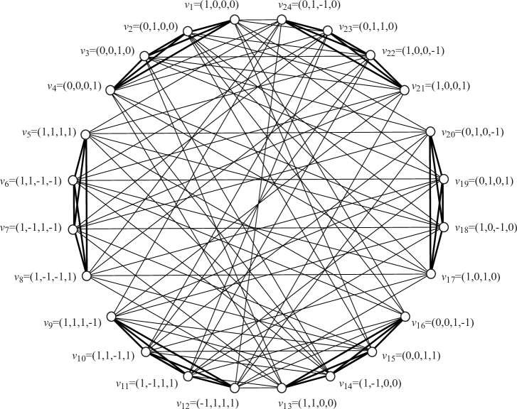
6.2.2 Pauli-
Fig. 1 shows the graph of orthogonality of the (not normalized) states in . This graph has and . Therefore, by preparing the maximally entangled state (12) of local dimension and allowing each of the parties to choose between the two-outcome measurements represented by , with , Alice and Bob can produce a violation of the Bell inequality (1) which, using Theorem 3, allows us to conclude that
| (54) |
and, using Theorem 7, allows us to conclude that
| (55) |
6.2.3 Gilbert’s algorithm
While our graph-based Bell inequalities are neither tight (i.e., facets of the local polytope) nor robust to noise, they can be further improved to offer better detection efficiency and noise robustness. This can be achieved by calculating the Bell functional in Eq. (3) using two different methods.
The first method is a linear program which optimizes over the entire local polytope to find the best Bell functional [27]. However, this technique requires enumerating and storing all the local deterministic points which are given by the vertices of the local polytope. This becomes an increasingly difficult computational task as the number of measurement settings increases. As an example, the local polytope corresponding to the Bell inequality with settings per party derived from has vertices. This number is too large to be stored on a standard computer. In this paper, we use a second method which is based on Gilbert’s distance algorithm [103] and does not require storing all the vertices of the local polytope. However, it should be noted that, for the cases we are interested in (e.g., ), the problem is still intractable using Gilbert’s original algorithm. The problem only becomes feasible when symmetries are also taken into account, as explained in Sec. 6.2.4.
Gilbert’s algorithm is a well-known numerical method to detect collisions between convex sets. It has been used for improving detection efficiencies of Bell inequalities [27], deciding whether or not a given correlation is nonlocal [104], and entanglement witnessing [105, 106]. The algorithm minimizes the distance between a local point on a facet of the local polytope and a nonlocal point specified by the user. The minimization is achieved by iteratively finding a better local point that minimizes this distance. The algorithm terminates when the difference of distances between successive iterations falls below a certain threshold value (typically taken to be extremely small). The resulting Bell functional is then identified as the separating hyperplane between the specified nonlocal point and the local point on the facet found by minimizing the distance. In the following, we will present this algorithm in more detail. The algorithm is based on an oracle which is capable of maximizing over the local polytope the inner product between a point in . Initially, one has to specify the local polytope , presented as the convex hull of vertices , and a point associated to the given quantum correlation. Then, the algorithm proceeds as follows. First, it chooses a point . Second, with the given point , it uses the oracle to compute
| (56) |
Third, given and , it calculates the convex combination of both which minimizes the distance to the quantum point , that is,
| (57) |
Since the objective function in (6.2.3) is linear and convex, the maximizer will be an extreme point of . In particular, will be a vertex of the local polytope . The optimal value for in the -th iteration, denoted by , can be computed directly and is given by
| (58) |
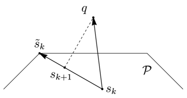
Then, it defines the new starting point to be and it proceeds with the second step. In the standard Gilbert’s algorithm, the oracle is implemented by enumerating all the vertices of the local polytope to compute the inner product in the last equality of Eq. (6.2.3). For a geometrical interpretation of the iteration of Gilbert’s algorithm, see Fig. 2.
This algorithm provides a sequence of Bell functionals, which become better with each iteration. Note that it does not necessarily provide a tight Bell inequality like the first method. Moreover, calculating the local bound of the resultant Bell functional still remains an NP hard problem, which again requires enumerating and storing all the local deterministic points at least for one party111For a given bipartite Bell functional where each measurement has only two outcomes , once we have fixed the deterministic assignment of one party, the optimal value of the Bell functional and the corresponding deterministic assignments of another party are determined. Refer to Sec. 1 in appendix C of Ref. [107] for more details.. This issue is also shared by the oracle in the standard Gilbert’s algorithm, since the evaluation of Eq. (6.2.3) is equivalent to find the local bound of one Bell functional.
6.2.4 Gilbert’s algorithm with symmetrization
The two problems mentioned at the end of the previous section can be solved simultaneously by replacing the hitherto generic oracle with an oracle that takes into account the symmetries of the problem. This provides an advantage that is crucial for improving the speed of convergence. In this respect, it is important to notice that the vertices of the local polytope (and the polytope itself) are invariant under the following invertible transformations: (i) Swapping the outcomes of a measurement setting for either Alice or Bob. (ii) Simultaneously permuting the measurement settings of Alice and Bob. (iii) Swapping the measurement settings of Alice and Bob. Here, “invariant” means that the transformations map local correlations to local correlations.
The joint probability distributions obtained by performing measurements on a quantum state are also invariant under some of these transformations. We denote by a subset of these transformations which keep the quantum joint probability distributions and the local polytope invariant simultaneously.
We consider a matrix similar to the one in Eq. (3) in which the entries are probability distributions instead of coefficients, given as,
| (63) |
The corresponding Bell inequality can then be calculated as . Under the transformations we have,
| (64) |
where is the resultant matrix after transformation . Therefore, we have
| (65) |
where
| (66) |
and is the cardinality of . Using this symmetry , it is sufficient to consider only inequalities that share this symmetry. In particular, for a symmetric inequality, the vertices of the local polytope can be partitioned into different equivalence classes with respect to that symmetry and the local bound can be computed by choosing only one representative out of each class. This drastically reduces the total number of local vertices required, allowing us to enumerate all symmetrized local points and evaluate the local bound.
For convenience, here we focus on the symmetrization applied only to Alice’s measurement settings. Each equivalence class consists of vertices which can be transformed into each other by using the aforementioned symmetry transformations, while the same is not true for vertices in different equivalence classes, i.e., the partition generates disjoint sets. This leads to a modified oracle, which is much more efficient than the original one since the number of equivalence classes could much smaller than the number of all vertices. This is indeed the case for .
Now, we describe how to obtain the reduced set of vertices on which the optimization in (6.2.3) has to run. In the first step, we have to determine the allowed symmetry transformations , which should be shared by the chosen quantum point and the local polytope . As already pointed out, is invariant under the permutation of parties, the permutation of the measurements for each party, and the permutation of the outcomes for each measurement. By construction, the chosen quantum point is also invariant under the permutation of parties. Usually, can change after the permutation of outcomes for each measurement. In general, determining the permutation symmetries of measurements in the point can be difficult when the number of measurements is large. In the cases considered here, those symmetry transformations correspond to the ones in the automorphism group of the graph associated to the SI-C sets. Therefore, the symmetry transformations used in the Gilbert’s algorithm with symmetrization are the ones in the automorphism group and the permutation of parties. It remains to explain how the vertices are partitioned into different equivalence classes.
The first important observation is that now we do not need to generate, store, and classify all vertices, since assignments with different number of ’s cannot be equivalent to each other. Hence, we can do the classification inductively. We start with the assignment that only contains ’s. Obviously, this is invariant under all possible permutations. From this, we generate all possible assignments that can be obtained by replacing one by one . Within this set, we check whether some of these assignments are equivalent under the given symmetry transformations , which are presented as permutations. Then, we only keep one representative for each class. This procedure is repeated until no is left in the assignment vector.
Selecting only a single vertex from each equivalence class (and all the vertices of Bob), we find that the total number of deterministic assignments for Alice is for the Bell inequality corresponding to (while, without symmetrization, it would be ).
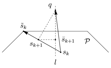
We also modify the Gilbert’s algorithm to evaluate the Bell functional according to the symmetrization procedure in Eq. (65). Specifically, we symmetrize the local point chosen in each iteration of the program after minimizing its distance from the target nonlocal point, see Fig. 3 for a simple illustration. This results in better convergence times of the algorithm since symmetrization does not increase the distance.
6.2.5 Example: Bell inequality for Pauli- that minimizes and
As an example, here we present a Bell functional for the correlations produced by the maximal entangled state (12), with , and the measurements associated to the states in which has lower detection efficiency and larger tolerance to white noise than those of to the graph-based Bell functional (1). The purpose of this example is to show that the values of and obtained in the first step of the method can, in principle, always be improved.
Applying Gilbert’s algorithm and the symmetrization technique to the correlations produced by and maximally entangled states, we have obtained the following Bell inequality:
| (67) |
where
| (68) |
with to be a matrix full of ’s, to be a vector full of ’s, and
| (69) |
where .
For the maximally entangled state (12), the quantum value is
| (70) |
In addition, for the correlations produced by and maximally entangled states,
| (71) |
which is lower than the upper bound in (55), and
| (72) |
which is lower than the upper bound in (54).
We can prove that and are the smallest possible values for the correlations produced by and maximally entangled states as follows: First, we collect all the pairs of deterministic assignments for the two parties which achieve the maximal bound for LHV models. Each of them corresponds to a matrix . After symmetrization, there are only different matrices , whose convex combination can lead to the corresponding quantum probability matrix either with or with , as one can verify with linear programming. Inequality (67) is not tight. There is a tight Bell inequality providing the same and than the ones for inequality (67), but it does not have the two blocks of ’s that we have in (69). If we want to keep the ’s, inequality (67) is the only solution.
Notice that symmetries of the initial graph are crucial for finding (69). For example, notice that there are only different parameters in the symmetric inequality for the case of . In comparison, there are parameters in the nonsymmetric inequality for . In the general case, there are parameters in the symmetric inequality for and . This makes it also possible to find a better inequality without resorting to Gilbert’s method. To be more explicit, we can choose different values for each parameter, then there are different inequalities. For each inequality, we can verify whether it separates the target quantum point and the LHV polytope or not by considering only the deterministic assignments up to symmetry. As discussed before, when , there are different deterministic assignments for Alice up to symmetry. Therefore, for a fixed inequality, this verification can be done very fast. Similarly, we can calculate and for each inequality. As we can see in Eq. (69), we can set some parameters to be for the best and . This trick can speed up the numerical calculation further.
7 Towards high-dimensional long-distance loophole-free Bell tests
We have shown how to identify quantum correlations between systems of moderate dimension () that allow for loophole-free Bell nonlocality with low detection efficiency. Our results imply that, probably, loophole-free Bell nonlocality can be achieved in carefully designed tests involving pairs of systems of these dimensions, which is interesting by itself as it goes beyond previous loophole-free Bell tests, all of them based on qubits. More interestingly, our results also imply that loophole-free Bell nonlocality can be achieved through longer distances than those of previous loophole-free Bell tests. When photons propagate thorough fibers, they experience propagation losses proportional to the propagation distance and which depend on the optical wavelength. This means that in a Bell test over long distances (and unless we add, e.g., heralded qudit amplifiers [39] or split each photon into two [41, 42] before the local measurements), the detection efficiency decreases with the distance. For example, with telecom wavelengths, in km of fiber, we may have losses of dB/km, which implies multiplying by the detection efficiency that we had before adding km of fiber. Therefore, if we have examples of loophole-free Bell nonlocality requiring , we can achieve loophole-free nonlocality over km if we have before adding the km of fiber. Such has been achieved in previous photonic loophole-free experiments [14, 15], even including ( m of) fibers and the couplings.
In this paper, we have shown how to achieve with local dimensions [see Eq. (20)] and how to obtain Bell inequalities with even lower and higher resistance to noise. Now the question is what are the values of the visibility that are experimentally achievable for the required configurations. Although some previous results are very promising [102], it is not clear to us whether similar values () can be achieved for the states and measurements described in this paper. For further progress, we need to know what pairs can be obtained for the type of states and measurements proposed here (e.g., for and Pauli-). In addition, we have introduced methods to identify further examples with low requiring smaller number of settings.
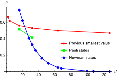
As shown in Fig. 4, the first step of our method already yields upper bounds for which are substantially smaller than the lowest values previously known for any dimension . These values indicate that there are quantum correlations which have sufficiently low for loophole-free Bell tests with higher-dimensional quantum systems and, eventually, over longer distances. We have also shown how to improve any of these values and we have described how we are trying to find more, and probably better, examples in the future.
It now remains to be seen how far we can go on the experimental side. In particular, there is one question, to which we do not have the answer: Is there a way to encode high-dimensional entanglement in photons that allows, at the same time, (i) to measure all the necessary one-dimensional projectors locally and switch quickly between them, (ii) distribute the photons over, e.g., – km achieving visibilities , (iii) using superconducting detectors to actually achieve ? Hopefully, the combination of techniques presented here and the interaction with experimental groups will help us to produce high-dimensional loophole-free Bell nonlocality over long distances in the near future.
The code supporting the results reported in this paper is available in [108].
Acknowledgments
We thank Ernesto Galvão, Junior R. Gonzales-Ureta, Petr Lisoněk, Debashis Saha, and Stefan Trandafir for discussions, and the University of Siegen for enabling our computations through the OMNI cluster. This work is supported by Universidad de Sevilla Project Qdisc (Project No. US-15097), with FEDER funds, MCINN/AEI Projet No. PID2020-113738GB-I00, QuantERA grant SECRET, by MCINN/AEI (Project No. PCI2019-111885-2), Deutsche Forschungsgemeinschaft (DFG, German Research Foundation, Project No. 447948357 and No. 440958198), the Sino-German Center for Research Promotion (Project No. M-0294), and the ERC (Consolidator Grant 683107/TempoQ). ZPX is supported by the Humboldt Foundation. JS is supported by the House of Young Talents of the University of Siegen. JRP is supported by Universidad de Sevilla Project No. US-1254251, with FEDER funds, and Junta de Andalucía Project No. P20-00592.
References
- [1] J. S. Bell, On the Einstein Podolsky Rosen paradox, Physics 1, 195 (1964).
- [2] N. Brunner, D. Cavalcanti, S. Pironio, V. Scarani, and S. Wehner, Bell nonlocality, Rev. Mod. Phys. 86, 419 (2014).
- [3] P. M. Pearle, Hidden-variable example based upon data rejection, Phys. Rev. D 2, 1418 (1970).
- [4] As explained in Ref. [3].
- [5] R. Colbeck, Quantum and Relativistic Protocols for Secure Multi-Party Computation, PhD thesis, University of Cambridge, 2006; arXiv:0911.3814.
- [6] S. Pironio, A. Acín, S. Massar, A. Boyer de la Giroday, D. N. Matsukevich, P. Maunz, S. Olmschenk, D. Hayes, L. Luo, T. A. Manning, and C. Monroe, Random numbers certified by Bell’s theorem, Nature 464, 1021 (2010).
- [7] W.-Z. Liu, M.-H. Li, S. Ragy, S.-R. Zhao, B. Bai, Y. Liu, P. J. Brown, J. Zhang, R. Colbeck, J. Fan, Q. Zhang, and J.-W. Pan, Device-independent randomness expansion against quantum side information, Nat. Phys. 17, 448 (2021).
- [8] L. K. Shalm, Y. Zhang, J. C. Bienfang, C. Schlager, M. J. Stevens, M. D. Mazurek, C. Abellán, W. Amaya, M. W. Mitchell, M. A. Alhejji, H. Fu, J. Ornstein, R. P. Mirin, S. W. Nam, and E. Knill, Device-independent randomness expansion with entangled photons, Nat. Phys. 17, 452 (2021).
- [9] A. K. Ekert, Quantum cryptography based on Bell’s theorem, Phys. Rev. Lett. 67, 661 (1991).
- [10] D. Mayers and A. Yao, Quantum cryptography with imperfect apparatus, Proceedings 39th Annual Symposium on Foundations of Computer Science (IEEE, Los Alamitos, CA, 1998), p. 503.
- [11] J. Barrett, L. Hardy, and A. Kent, No signaling and quantum key distribution, Phys. Rev. Lett. 95, 010503 (2005).
- [12] A. Acín, N. Brunner, N. Gisin, S. Massar, S. Pironio, and V. Scarani, Device-independent security of quantum cryptography against collective attacks, Phys. Rev. Lett. 98, 230501 (2007).
- [13] S. Pironio, A. Acín, N. Brunner, N. Gisin, S. Massar, and V. Scarani, Device-independent quantum key distribution secure against collective attacks, New J. Phys. 11, 045021 (2009).
- [14] M. Giustina, M. A. M. Versteegh, S. Wengerowsky, J. Handsteiner, A. Hochrainer, K. Phelan, F. Steinlechner, J. Kofler, J.-Å. Larsson, C. Abellán, W. Amaya, V. Pruneri, M. W. Mitchell, J. Beyer, T. Gerrits, A. E. Lita, L. K. Shalm, S. W. Nam, T. Scheidl, R. Ursin, B. Wittmann, and A. Zeilinger, Significant-loophole-free test of Bell’s theorem with entangled photons, Phys. Rev. Lett. 115, 250401 (2015).
- [15] L. K. Shalm, E. Meyer-Scott, B. G. Christensen, P. Bierhorst, M. A. Wayne, M. J. Stevens, T. Gerrits, S. Glancy, D. R. Hamel, M. S. Allman, K. J. Coakley, S. D. Dyer, C. Hodge, A. E. Lita, V. B. Verma, C. Lambrocco, E. Tortorici, A. L. Migdall, Y. Zhang, D. R. Kumor, W. H. Farr, F. Marsili, M. D. Shaw, J. A. Stern, C. Abellán, W. Amaya, V. Pruneri, T. Jennewein, M. W. Mitchell, P. G. Kwiat, J. C. Bienfang, R. P. Mirin, E. Knill, and S. W. Nam, Strong loophole-free test of local realism, Phys. Rev. Lett. 115, 250402 (2015).
- [16] W. Rosenfeld, D. Burchardt, R. Garthoff, K. Redeker, N. Ortegel, M. Rau, and H. Weinfurter, Event-ready Bell test using entangled atoms simultaneously closing detection and locality loopholes, Phys. Rev. Lett. 119, 010402 (2017).
- [17] B. Hensen, H. Bernien, A. E. Dréau, A. Reiserer, N. Kalb, M. S. Blok, J. Ruitenberg, R. F. L. Vermeulen, R. N. Schouten, C. Abellán, W. Amaya, V. Pruneri, M. W. Mitchell, M. Markham, D. J. Twitchen, D. Elkouss, S. Wehner, T. H. Taminiau, and R. Hanson, Loophole-free Bell inequality violation using electron spins separated by 1.3 kilometres, Nature 526, 682 (2015).
- [18] I. Pitowsky, Quantum Probability – Quantum Logic, Lecture Notes in Physics 321 (Springer, Berlin, 1989).
- [19] A. Garg and N. D. Mermin, Detector inefficiencies in the Einstein-Podolsky-Rosen experiment, Phys. Rev. D 35, 3831 (1987).
- [20] J. F. Clauser, M. A. Horne, A. Shimony, and R. A. Holt, Proposed experiment to test local hidden-variable theories, Phys. Rev. Lett. 23, 880 (1969).
- [21] P. H. Eberhard, Background level and counter efficiencies required for a loophole-free Einstein-Podolsky-Rosen experiment, Phys. Rev. A 47, R747(R) (1993).
- [22] J. F. Clauser and M. A. Horne, Experimental consequences of objective local theories, Phys. Rev. D. 10 526 (1974).
- [23] N. Brunner and N. Gisin, Partial list of bipartite Bell inequalities with four binary settings, Phys. Lett. A 372, 3162 (2008).
- [24] E. Zambrini Cruzeiro and N. Gisin, Complete list of tight Bell inequalities for two parties with four binary settings, Phys. Rev. A 99, 022104 (2019).
- [25] S. Massar, Nonlocality, closing the detection loophole, and communication complexity, Phys. Rev. A 65, 032121 (2002).
- [26] T. Vértesi, S. Pironio, and N. Brunner, Closing the detection loophole in Bell experiments using qudits, Phys. Rev. Lett. 104, 060401 (2010).
- [27] I. Márton, E. Bene, and T. Vértesi, Bounding the detection efficiency threshold in Bell tests using multiple copies of the two-qubit maximally entangled state, Phys. Rev. A 107, 022205 (2023).
- [28] N. Miklin, A. Chaturvedi, M. Bourennane, M. Pawłowski, and A. Cabello, Exponentially decreasing the critical detection efficiency for any Bell inequality, Phys. Rev. Lett. 129, 230403 (2022).
- [29] J.-Å. Larsson and J. Semitecolos, Strict detector-efficiency bounds for -site Clauser-Horne inequalities, Phys. Rev. A 63, 022117 (2001).
- [30] A. Cabello, D. Rodríguez, and I. Villanueva, Necessary and sufficient detection efficiency for the Mermin inequalities, Phys. Rev. Lett. 101, 120402 (2008).
- [31] K. F. Pál, T. Vértesi, and N. Brunner, Closing the detection loophole in multipartite Bell tests using Greenberger-Horne-Zeilinger states, Phys. Rev. A 86, 062111 (2012).
- [32] A. Cabello and J.-Å. Larsson, Minimum detection efficiency for a loophole-free atom-photon Bell experiment, Phys. Rev. Lett. 98, 220402 (2007).
- [33] N. Brunner, N. Gisin, V. Scarani, and C. Simon, Detection loophole in asymmetric Bell experiments, Phys. Rev. Lett. 98, 220403 (2007).
- [34] G. Garbarino, Minimum detection efficiencies for a loophole-free observable-asymmetric Bell-type test, Phys. Rev. A 81, 032106 (2010).
- [35] M. Araújo, M. T. Quintino, D. Cavalcanti, M. França Santos, A. Cabello, and M. Terra Cunha, Tests of Bell inequality with arbitrarily low photodetection efficiency and homodyne measurements, Phys. Rev. A 86, 030101(R) (2012).
- [36] J. Å. Larsson, Loopholes in Bell inequality tests of local realism, J. Phys. A: Math. Theor. 47, 424003 (2014).
- [37] J. Hofmann, M. Krug, N. Ortegel, L. Gérard, M. Weber, W. Rosenfeld, and H. Weinfurter, Heralded entanglement between widely separated atoms, Science 337, 72 (2012).
- [38] T. C. Ralph and A. P. Lund, Nondeterministic noiseless linear amplification of quantum systems, AIP Conference Proceedings 1110, 155 (2009).
- [39] N. Gisin, S. Pironio, and N. Sangouard, Proposal for implementing device-independent quantum key distribution based on a heralded qubit amplifier, Phys. Rev. Lett. 105, 070501 (2010).
- [40] C. Branciard, Detection loophole in Bell experiments: How postselection modifies the requirements to observe nonlocality, Phys. Rev. A 83, 032123 (2011).
- [41] A. Cabello and F. Sciarrino, Loophole-free Bell test based on local precertification of photon’s presence, Phys. Rev. X 2, 021010 (2012).
- [42] E. Meyer-Scott, D. McCloskey, K. Gołos, J. Z. Salvail, K. A. G. Fisher, D. Hamel, A. Cabello, K. J. Resch, and T. Jennewein, Certifying the presence of a photonic qubit by splitting it in two, Phys. Rev. Lett. 116, 070501 (2016).
- [43] M. Giustina, A. Mech, S. Ramelow, B. Wittmann, J. Kofler, J. Beyer, A. Lita, B. Calkins, T. Gerrits, S. W. Nam, R. Ursin, and A. Zeilinger, Bell violation using entangled photons without the fair-sampling assumption, Nature 497, 227 (2013).
- [44] B. G. Christensen, K. T. McCusker, J. B. Altepeter, B. Calkins, T. Gerrits, A. E. Lita, A. Miller, L. K. Shalm, Y. Zhang, S. W. Nam, N. Brunner, C. C. W. Lim, N. Gisin, and P. G. Kwiat, Detection-loophole-free test of quantum nonlocality, and applications, Phys. Rev. Lett. 111, 130406 (2013).
- [45] Y. Liu, X. Yuan, M. Li, W. Zhang, Q. Zhao, J. Zhong, Y. Cao, Y.-H. Li, L.-K. Chen, H. Li, T. Peng, Y.-A. Chen, C. Peng, S.-C. Shi, Z. Wang, L. You, X. Ma, J. Fan, Q. Zhang, and J.-W. Pan, High-speed device-independent quantum random number generation without a detection loophole, Phys. Rev. Lett. 120, 010503 (2018).
- [46] L. Shen, J. Lee, L. P. Thinh, J.-D. Bancal, A. Cerè, A. Lamas-Linares, A. Lita, T. Gerrits, S. W. Nam, V. Scarani, and C. Kurtsiefer, Randomness extraction from Bell violation with continuous parametric down-conversion, Phys. Rev. Lett. 121, 150402 (2018).
- [47] P. Bierhorst, E. Knill, S. Glancy, Y. Zhang, A. Mink, S. Jordan, A. Rommal, Y.-K. Liu, B. Christensen, S. W. Nam, M. J. Stevens, and L. K. Shalm, Experimentally generated randomness certified by the impossibility of superluminal signals, Nature 556, 223 (2018).
- [48] Y. Liu, Q. Zhao, M.-H. Li, J.-Y. Guan, Y. Zhang, B. Bai, W. Zhang, W.-Z. Liu, C. Wu, X. Yuan, H. Li, W. J. Munro, Z. Wang, L. You, J. Zhang, X. Ma, J. Fan, Q. Zhang, and J.-W. Pan, Device-independent quantum random-number generation, Nature 562, 548 (2018).
- [49] M.-H. Li, C. Wu, Y. Zhang, W.-Z. Liu, B. Bai, Y. Liu, W. Zhang, Q. Zhao, H. Li, Z. Wang, L. You, W. J. Munro, J. Yin, J. Zhang, C.-Z. Peng, X. Ma, Q. Zhang, J. Fan, and J.-W. Pan, Test of local realism into the past without detection and locality loopholes, Phys. Rev. Lett. 121, 080404 (2018).
- [50] Y. Zhang, L. K. Shalm, J. C. Bienfang, M. J. Stevens, M. D. Mazurek, S. W. Nam, C. Abellán, W. Amaya, M. W. Mitchell, H. Fu, C. A. Miller, A. Mink, and E. Knill, Experimental low-latency device-independent quantum randomness, Phys. Rev. Lett. 124, 010505 (2020).
- [51] L. K. Shalm, Y. Zhang, J. C. Bienfang, C. Schlager, M. J. Stevens, M. D. Mazurek, C. Abellán, W. Amaya, M. W. Mitchell, M. A. Alhejji, H. Fu, J. Ornstein, R. P. Mirin, S. W. Nam, and E. Knill, Device-independent randomness expansion with entangled photons, Nat. Phys. 17, 452 (2021).
- [52] M.-H. Li, X. Zhang, W.-Z. Liu, S.-R. Zhao, B. Bai, Y. Liu, Q. Zhao, Y. Peng, J. Zhang, Y. Zhang, W. J. Munro, X. Ma, Q. Zhang, J. Fan, and J.-W. Pan, Experimental realization of device-independent quantum randomness expansion, Phys. Rev. Lett. 126, 050503 (2021).
- [53] W.-Z. Liu, M.-H. Li, S. Ragy, S.-R. Zhao, B. Bai, Y. Liu, P. J. Brown, J. Zhang, R. Colbeck, J. Fan, Q. Zhang, and J.-W. Pan, Device-independent randomness expansion against quantum side information, Nat. Phys. 17, 448 (2021).
- [54] W.-Z. Liu, Y.-Z. Zhang, Y.-Z. Zhen, M.-H. Li, Y. Liu, J. Fan, F. Xu, Q. Zhang, and J.-W. Pan, Photonic verification of device-independent quantum key distribution against collective attacks, Phys. Rev. Lett. 129, 050502 (2022).
- [55] J.-L. Chen, A. Cabello, Z.-P. Xu, H.-Y. Su, C. Wu, and L. C. Kwek, Hardy’s paradox for high-dimensional systems, Phys. Rev. A 88, 062116 (2013).
- [56] T. K. Lo and A. Shimony, Proposed molecular test of local hidden-variables theories, Phys. Rev. A 23, 3003 (1981).
- [57] D. Collins and N. Gisin, A relevant two qubit Bell inequality inequivalent to the CHSH inequality, J. Phys. A: Math. Gen. 37, 1775 (2004).
- [58] R. Diestel, Graph Theory, Graduate Texts in Mathematics 173 (Springer, Berlin, 2017).
- [59] L. Hogben, K. F. Palmowski, D. E. Roberson, and S. Severini, Orthogonal representations, projective rank, and fractional minimum positive semidefinite rank: Connections and new directions, Electron. J. Linear Algebra 32, 98 (2017).
- [60] L. Lovász, On the Shannon capacity of a graph, IEEE Trans. Inf. Theory 25, 1 (1979).
- [61] M. Grötschel, L. Lovász, and A. Schrijver, Relaxations of vertex packings, J. Combin. Theory B 40, 330 (1986).
- [62] C. E. Shannon, The zero-error capacity of a noisy channel. IRE Trans. Inform. Theory 2, 8 (1956).
- [63] A. Cabello, S. Severini, and A. Winter, (Non-)Contextuality of physical theories as an axiom, Mittag-Leffler-2010fall Report No. 8 (2010).
- [64] M. Planat, Quantum states arising from the Pauli groups, symmetries and paradoxes, in Symmetries and Groups in Contemporary Physics. Proceedings of the XXIX International Colloquium on Group-Theoretical Methods in Physics, edited by C. Bai, J.-P. Gazeau, and M. L. Ge, Nankai Series in Pure, Applied Mathematics and Theoretical Physics 11 (World Scientific, Singapore, 2013), p. 295.
- [65] M. W. Newman, Independent Sets and Eigenspaces, Ph.D. thesis, University of Waterloo, 2004.
- [66] M. Reck, A. Zeilinger, H. J. Bernstein, and P. Bertani, Experimental realization of any discrete unitary operator, Phys. Rev. Lett. 73, 58 (1994).
- [67] W. R. Clements, P. C. Humphreys, B. J. Metcalf, W. S. Kolthammer, and I. A. Walmsley, Optimal design for universal multiport interferometers, Optica 3, 1460 (2016).
- [68] M. C. Tichy, M. Tiersch, F. de Melo, F. Mintert, and A. Buchleitner, Zero-transmission law for multiport beam splitters, Phys. Rev. Lett. 104, 220405 (2010).
- [69] A. Crespi, Suppression laws for multiparticle interference in Sylvester interferometers, Phys. Rev. A 91, 013811 (2015).
- [70] N. Ito, Hadamard graphs. I, Graphs Comb. 1, 57 (1985).
- [71] N. Ito, Hadamard graphs. II, Graphs Comb. 1, 331 (1985).
- [72] G. Brassard, R. Cleve, and A. Tapp, The cost of exactly simulating quantum entanglement with classical communication, Phys. Rev. Lett. 83, 1874 (1999).
- [73] V. Galliard, A. Tapp, and S. Wolf, Deterministic quantum non-locality and graph colorings, Theor. Comput. Sci. 486, 20 (2013).
- [74] D. Avis, A quantum protocol to win the graph colouring game on all Hadamard graphs, IEICE Trans. Fundam. Electron. Commun. Comput. Sci. 89, 1378 (2006).
- [75] P. J. Cameron, A. Montanaro, M. W. Newman, S. Severini, and A. Winter, On the quantum chromatic number of a graph, Electron. J. Comb. 14, R81 (2007).
- [76] G. Scarpa and S. Severini, Kochen-Specker sets and the rank-1 quantum chromatic number, IEEE Trans. Inf. Theory 58, 2524 (2012).
- [77] L. Mančinska and D. E. Roberson, Quantum homomorphisms, J. Combin. Theory Ser. B 118, 228 (2016).
- [78] P. Wocjan and C. Elphick, Spectral lower bounds for the orthogonal and projective ranks of a graph, Electron. J. Comb. 26, 3.45 (2019).
- [79] P. Frankl, Orthogonal vectors in the -dimensional cube and codes with missing distances, Combinatorica 6, 279 (1986).
- [80] F. Ihringer and H. Tanaka, The independence number of the orthogonality graph in dimension , Combinatorica 39, 1425 (2019).
- [81] J. J. Sylvester, Thoughts on inverse orthogonal matrices, simultaneous sign successions, and tessellated pavements in two or more colours, with applications to Newton’s rule, ornamental tile-work, and the theory of numbers, Philos. Mag. 34, 461 (1867).
- [82] R. E. A. C. Paley, On orthogonal matrices, J. Math. Phys. 4, 311 (1933).
- [83] H. Kimura, Classification of Hadamard matrices of order 28, Discrete Math. 133, 171 (1994).
- [84] B. D. McKay, Topics in Computational Graph Theory, Ph.D. thesis, University of Melburne, 1980.
- [85] A. Cabello, M. Kleinmann, and C. Budroni, Necessary and sufficient condition for quantum state-independent contextuality, Phys. Rev. Lett. 114, 250402 (2015).
- [86] D. E. Knuth, The sandwich theorem, Electron. J. Combin. 1, A1 (1994).
- [87] R. J. Nowakowski and D. F. Rall, Associative graph products and their independence, domination and coloring numbers, Discuss. Math. Graph Theory 16, 53 (1996).
- [88] D. Geller and S. Stahl, The chromatic number and other functions of the lexicographic product, J. Comb. Theory. Ser. B 19, 87 (1975).
- [89] D. E. Roberson, Conic formulations of graph homomorphisms, J. Algebr. Comb. 43, 877 (2016).
- [90] G. F. Royle, and C. E. Praeger, Constructing the vertex-transitive graphs of order 24, J. Symb. Comput. 8, 4 (1989).
- [91] B. D. McKay and G. F. Royle, The transitive graphs with at most 26 vertices, Ars Combin. 30, 161 (1990).
- [92] D. Holt and G. Royle, A census of small transitive groups and vertex-transitive graphs, J. Symb. Comput. 101, (2020).
- [93] P. Potočnik, P. Spiga, and G. Verret, Cubic vertex-transitive graphs on up to 1280 vertices, J. Symb. Comput. 50, (2013).
- [94] B. D. McKay, Graphs.
- [95] L. Lovász, Graphs and Geometry, Institute of Mathematics, Ëotvös University, Budapest, 2019.
- [96] Z.-P. Xu, X.-D. Yu, and M. Kleinmann, State-independent quantum contextuality with projectors of nonunit rank, New J. Phys. 23, 043025 (2021).
- [97] A. Cabello, Converting contextuality into nonlocality, Phys. Rev. Lett. 127, 070401 (2021).
- [98] S. Yu and C. H. Oh, State-independent proof of Kochen-Specker theorem with 13 rays, Phys. Rev. Lett. 108, 030402 (2012).
- [99] A. Cabello, M. Kleinmann, and J. R. Portillo, Quantum state-independent contextuality requires 13 rays, J. Phys. A: Math. Theor. 49, 38LT01 (2016).
- [100] A. Cabello, Á. Feito, and A. Lamas-Linares, Bell’s inequalities with realistic noise for polarization-entangled photons Phys. Rev. A 72, 052112 (2005).
- [101] F. A. Bovino, G. Castagnoli, A. Cabello, and A. Lamas-Linares, Experimental noise-resistant Bell-inequality violations for polarization-entangled photons, Phys. Rev. A 73, 062110 (2006).
- [102] N. Herrera Valencia, V. Srivastav, M. Pivoluska, M Huber, N. Friis, W. McCutcheon, and M. Malik, High-dimensional pixel entanglement: Efficient generation and certification, Quantum 4, 376 (2020).
- [103] E. G. Gilbert, An iterative procedure for computing the minimum of a quadratic form on a convex set, J. SIAM Control 4, 61 (1966).
- [104] A. Montina and S. Wolf, Discrimination of non-local correlations, Entropy 21, 104 (2019).
- [105] J. Shang and O. Gühne, Convex optimization over classes of multiparticle entanglement, Phys. Rev. Lett. 120, 050506 (2018).
- [106] P. Pandya, O. Sakarya, and M. Wieśniak, Hilbert-Schmidt distance and entanglement witnessing, Phys. Rev. A 102, 012409 (2020).
- [107] J. R. Gonzales-Ureta, A. Predojević and A. Cabello, Optimal and tight Bell inequalities for state-independent contextuality sets, arXiv:2207.08850
- [108] Z.-P. Xu, J. Steinberg, J. Singh, A. J. López-Tarrida, J. R. Portillo, and A. Cabello, Code to accompany Graph-theoretic approach to Bell experiments with low detection efficiency, https://gitlab.com/JoStei1996/symmetric_bell.
