ALLSH: Active Learning Guided by Local Sensitivity and Hardness

Abstract

Active learning, which effectively collects informative unlabeled data for annotation, reduces the demand for labeled data. In this work, we propose to retrieve unlabeled samples with a local sensitivity and hardness-aware acquisition function. The proposed method generates data copies through local perturbations and selects data points whose predictive likelihoods diverge the most from their copies. We further empower our acquisition function by injecting the select-worst case perturbation. Our method achieves consistent gains over the commonly used active learning strategies in various classification tasks. Furthermore, we observe consistent improvements over the baselines on the study of prompt selection in prompt-based few-shot learning. These experiments demonstrate that our acquisition guided by local sensitivity and hardness can be effective and beneficial for many NLP tasks.

1 Introduction

Crowdsourcing annotations Rajpurkar et al. (2016); Bowman et al. (2015) has become a common practice for developing NLP benchmark datasets. Rich prior works Pavlick and Kwiatkowski (2019); Nie et al. (2020); Ferracane et al. (2021) show that the time-consuming and expensive manual labeling in crowdsourcing annotations are not an annotation artifact but rather core linguistic phenomena. Active Learning (AL) is introduced to efficiently acquire data for annotation from a (typically large) pool of unlabeled data. Its goal is to concentrate the human labeling effort on the most informative data in hopes of maximizing the model performance while minimizing the data annotation cost.

Popular approaches to acquiring data for AL are uncertainty sampling and diversity sampling. Uncertainty sampling selects data that the model predicts with low-confidence Lewis and Gale (1994); Culotta and McCallum (2005); Settles (2009). Diversity sampling selects batches of unlabeled examples that are prototypical of the unlabeled pool to exploit heterogeneity in the feature space Xu et al. (2003); Bodó et al. (2011). Different from these two perspectives, recent works focus on the informativeness of the selected data. For example, Zhang and Plank (2021) acquire informative unlabeled data using the training dynamics based on the model predictive log likelihood. Margatina et al. (2021) construct contrastive examples in the input feature space. However, these methods either ignore the local sensitivity of the input features or take no consideration of the difficulty of the learning data. Consequently, they may ignore examples around the decision boundary, or select hard-to-train or even noisy examples. Their performance may further suffer under some practical settings, such as those with imbalanced labels and when there is a very limited annotation budget.

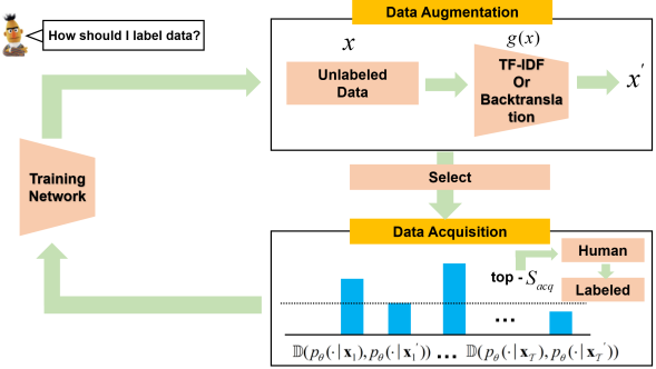
Figure 1: Overview of active learning framework guided by local sensitivity and hardness. Some notations are labeled along with corresponding components. ‘Select’ refers to the select worst-case augmentation.

In this work, we determine the informativeness by considering both the local sensitivity and learning difficulty. For local sensitivity, we take the classical definition from Chapelle et al. (2009), which is widely used in both classic machine learning problems (e.g. Blum and Chawla, 2001; Chapelle et al., 2002; Seeger, 2000; Zhu et al., 2003; Zhou et al., 2004) and recent deep learning settings (e.g. Wang et al., 2018b; Sohn et al., 2020; Xu et al., 2021). Specifying a local region $\mathcal{R}_{\textit{region}}(\boldsymbol{x})$ around an example $\boldsymbol{x}$, we assume in our prior that all examples in $\mathcal{R}_{\textit{region}}(\boldsymbol{x})$ have the same labels. If the examples in $\mathcal{R}_{\textit{region}}(\boldsymbol{x})$ give us different labels, we say the local region of $\boldsymbol{x}$ is sensitive. Data augmentation has been chosen as the way to create label-equivalent local regions in many recent works ($e.g.$, Berthelot et al., 2019b; Xie et al., 2020). We utilize data augmentation as a tool to capture the local sensitivity and hardness of inputs and present ALLSH: Active Learning guided by Local Sensitivity and Hardness. Through various designs on local perturbations, ALLSH selects unlabeled data points from the pool whose predictive likelihoods diverge the most from their augmented copies. This way, ALLSH can effectively ensure the informative and local-sensitive data to have correct human-annotated labels. Figure 1 illustrates the scheme of the proposed acquisition strategy.

We conduct a comprehensive evaluation of our approach on datasets ranging from sentiment analysis, topic classification, natural language inference, to paraphrase detection. To measure the proposed acquisition function in more realistic settings where the samples stem from a dissimilar input distribution, we (1) set up an out-of-domain test dataset and (2) leak out-of-domain data ($e.g.$, adversarial perturbations) into the selection pool.

We further expand the proposed acquisition to a more challenging setting: prompt-based few-shot learning Zhao et al. (2021), where we query a fixed pre-trained language model via a natural language prompt containing a few training examples. We focus on selecting the most valuable prompts for a given test task ($e.g.$, selecting 4 prompts for one given dataset). We adapt our acquisition function to retrieve prompts for the GPT-2 model.

Furthermore, we provide extensive ablation studies on different design choices for the acquisition function, including the designs of augmentations and divergences. Our method shows consistent gains in all settings with multiple datasets. With little modification, our data acquisition can be easily applied to other NLP tasks for a better sample selection strategy.

Our contributions are summarized as follows: (1) Present a new acquisition strategy, embracing local sensitivity and learning difficulty, such as paraphrasing the inputs through data augmentation and adversarial perturbations, into the selection procedure. (2) Verify the effectiveness and general applicability of the proposed method in more practical settings with imbalanced datasets and extremely few labeled data. (3) Provide comprehensive study and experiments of the proposed selection criteria in classification tasks (both in-domain and out-of-domain evaluations) and prompt-based few-shot learning. (4) The proposed data sampling strategy can be easily incorporated or extended to many other NLP tasks.

2 Method

In this section we present in detail our proposed method, ALLSH (Algorithm 1).

2.1 Active Learning Loop

The active learning setup consists of an unlabeled dataset $\mathcal{D}_{pool}$, the current training set $\mathcal{D}_{label}$, and a model $\mathcal{M}$ whose output probability is $p_{\theta}(\cdot\mid\boldsymbol{x})$ for input $\boldsymbol{x}$. The model $\mathcal{M}$ is generally a pre-trained model for NLP tasks Lowell et al. (2018). At each iteration, we train a model on $\mathcal{D}_{label}$ and then use the acquisition function to acquire $s_{\textit{acq}}$ sentences in a batch $\mathcal{T}$ from $\mathcal{D}_{pool}$. The acquired examples from this iteration are labeled, added to $\mathcal{D}_{label}$, and removed from $\mathcal{D}_{pool}$. Then the updated $\mathcal{D}_{label}$ serves as the training set in the next AL iteration until we exhaust the budget. Overall, the system is given a budget of $S$ queries to build a labeled training dataset of size $S$.

2.2 Acquisition Function Design

To fully capture the data informativeness and train a model with a limited amount of data, we consider two data-selection principals: local sensitivity and learning hardness.

Local Sensitivity Based on theoretical works on the margin theory for active learning, the examples lying close to the decision boundary are informative and worth labeling Ducoffe and Precioso (2018); Margatina et al. (2021). Uncertainty sampling suffers from the sampling bias problem as the model is only trained with few examples in the early phase of training. In addition, high uncertainty samples given the current model state may not be that representative to the whole unlabeled data Ru et al. (2020). For example, if an input has high confidence while its local perturbation generates low-confidence output, then it is likely that this input lies close to the model decision boundary. This information can be captured by measuring the difference between an input example and its augmentation in the output feature space. We utilize the back-translation Sennrich et al. (2016); Edunov et al. (2018); Zhang et al. (2021b) and TF-IDF Xie et al. (2020) as effective augmentation methods which can generate diverse paraphrases while preserving the semantics of the original inputs Yu et al. (2018b).

Instead of simply using augmentation, adversarial perturbation can measure the local Lipschitz and sensitivity more effectively. We therefore further exploit adversarial perturbation to more accurately measure local sensitivity. For NLP problems, generating exact adversarial perturbations in a discrete space usually requires combinatorial optimization, which often suffers from the curse of dimensionality  (Madry et al., 2017; Lei et al., 2018). Hence, we choose the hardest augmentation over $K$ random augmentations as a “lightweight” variant of adversarial input augmentation which optimizes the worst case loss over the augmented data.

Learning Hardness: From Easy to Hard Learning from easy examples or propagating labels from high-confidence examples is the key principle for curriculum learning (Bengio et al., 2009) and label propagation based semi-supervised learning algorithms (Chapelle et al., 2009). For example, FixMatch (Sohn et al., 2020), a SOTA semi-supervised method, applies an indicator function to select high confident examples at each iteration. This will facilitate the label information from high confidence examples to low-confidence ones Chapelle et al. (2009). In our selection criterion, as the model is trained with limited data, we also want to avoid the hard-to-learn examples, which in some cases frequently correspond to mislabeled or erroneous instances Swayamdipta et al. (2020); Zhang and Plank (2021). These examples may stuck the model performance at the beginning of the selection.

2.3 Acquisition with Local Sensitivity and Hardness

We come to the definition of our acquisition function. Given a model $p_{\theta}$ and an input $\boldsymbol{x}$, we compute the output distribution $p_{\theta}(\cdot\mid\boldsymbol{x})$ and a noised version $p_{\theta}(\cdot\mid\boldsymbol{x}^{\prime})$ by injecting a random transformation $\boldsymbol{x}^{\prime}=g(\boldsymbol{x})$ to the inputs. Here, $g(\cdot)$ is sampled from a family of transformations and these random transformations stand for data augmentations. This procedure can select examples that are insensitive to transformation $g(\cdot)$ and hence smoother with respect to the changes in the input space Berthelot et al. (2019b, a); Sohn et al. (2020). We calculate

$$\ell(\boldsymbol{x},\boldsymbol{x}^{\prime})=\mathbb{D}(p_{\theta}(\cdot\mid\boldsymbol{x}),p_{\theta}(\cdot\mid\boldsymbol{x^{\prime}})),\vspace{-3mm}$$ (1)

where $\mathbb{D}$ denotes a statistical distance such as the Kullback–Leibler (KL) divergence Kullback and Leibler (1951). Model $p_{\theta}$ here can be a pretrained language model such as BERT Devlin et al. (2018).

Data Paraphrasing via Augmentation

Paraphrase generation can improve language models Yu et al. (2018a) by handling language variation. TF-IDF and backtranslation can generate diverse inputs while preserving the semantic meaning Singh et al. (2019); Xie et al. (2020). For TF-IDF, we replace uninformative words with low TF-IDF scores while keeping those with high. Specifically, Suppose IDF$(w)$ is the IDF score for word $w$ computed on the whole corpus, and TF$(w)$ is the TF score for word $w$ in a sentence. We compute the TF-IDF score as TFIDF$(w)=$ TF$(w)$IDF$(w)$. For backtranslation, we use a pre-trained EN-DE and DE-EN translation models Ng et al. (2019) to perform backtranslation on each sentence. We denote $\boldsymbol{x}$ as $(x_{0},\cdots,x_{n})$. Here, $n$ denotes the original length of the input. For $\boldsymbol{x}$, we pass them through two translation models to get $\boldsymbol{x}^{\prime}=(x^{\prime}_{0},\cdots,x^{\prime}_{m})$, where $m$ denotes the length after backtranslating. More details can be found in Appendix A.

Select Worst-Case Augmentation (WCA)

In order to construct effective local sensitivity, the most direct approach is calculating the local Lipschitz constant or finding the worst case adversarial perturbation. However, estimating the Lipschitz constant for a neural network is either model dependent or computationally hard (Scaman and Virmaux, 2018; Fazlyab et al., 2019). Instead, we select worst-case augmentation over $K$ copies, which can still roughly measure the norm of the first-order gradient without a huge computation cost and is easy to implement. Given input examples $\boldsymbol{x}$, and $K$ augmentation of $\boldsymbol{x}$ as $\{\boldsymbol{x}_{i}^{\prime}\}_{i=1}^{K}$, we propose the following acquisition function to select data:

$$\ell^{\textit{max}}(\boldsymbol{x})=\max_{i\in[K]}\ell(\boldsymbol{x},\boldsymbol{x}_{i}^{\prime}).\vspace{-3mm}$$ (2)

Inspired by some simple and informal analysis in continuous space, we draw the connection between calculating $\ell^{\textit{max}}(\boldsymbol{x})$ and local sensitivity by

$$\begin{split}&\leavevmode\resizebox{357.0112pt}{}{$\ell^{\textit{max}}(\boldsymbol{x})=\ell(\boldsymbol{x},\boldsymbol{x}^{\prime})+\bigg{[}\ell^{\textit{max}}(\boldsymbol{x})-\ell(\boldsymbol{x},\boldsymbol{x}^{\prime})\bigg{]}$}\\ &\leavevmode\resizebox{422.77661pt}{}{$=\ell(\boldsymbol{x},\boldsymbol{x}^{\prime})+\left[\max_{i\in[K]}\langle\nabla_{\boldsymbol{x}}\ell(\boldsymbol{x},\boldsymbol{x}^{\prime}),\boldsymbol{x}-\boldsymbol{x}^{\prime}\rangle\right]+\mathbf{O}(\sigma^{2}).$}\end{split}\!$$ (3)

Recent works in computer vision (Gong et al., 2020; Wang et al., 2021) have provided more formal connections between local gradient norm estimation and $K$-worst perturbations.

The text sentences in NLP are in the discrete space, which lacks the definition of local Lipschitz, but finding the worst perturbation in a local discrete set can still be a better measurement of local sensitivity in the semantic space.

Choice of Divergence We use the KL divergence as the primary measure of the statistical distance between the distribution of the original examples and that over augmented examples. We also empirically provide detailed analysis of the Jensen–Shannon Distance (JSD) Endres and Schindelin (2003) and $\alpha$-divergence Minka et al. (2005) as a complementary measure in Section 5. The $\alpha$-divergence Pillutla et al. (2021) is a general divergence family, which includes the most popular KL divergence and reverse KL divergence. Different value of $\alpha$ makes the divergence trade-off between overestimation and underestimation. JSD is a metric function based on a mathematical definition which is symmetric and bounded within the range $[0,1]$. These divergences are calculated as:

$$\begin{split}&\leavevmode\resizebox{234.87749pt}{}{${\mathrm{KL}}(p\|q)=\sum\limits_{i}p_{i}(\boldsymbol{x})\log\frac{p_{i}(\boldsymbol{x})}{q_{i}(\boldsymbol{x})},$}\\ &\leavevmode\resizebox{281.85585pt}{}{${\mathrm{JSD}}(p\|q)=\sqrt{\frac{1}{2}(\mathrm{KL}(p\|m)+\mathrm{KL}(q\|m))},$}\\ &\leavevmode\resizebox{281.85585pt}{}{$\mathrm{D}_{\alpha}(p\|q)=\frac{1}{\alpha(\alpha-1)}\sum\limits_{i}[(\frac{p_{i}(\boldsymbol{x})}{q_{i}(\boldsymbol{x})})^{\alpha}-1],$}\\ \end{split}$$ (4)

where $p$ is the output probability distribution of an example, $q$ is the output probability distribution of an augmented example, and $m=\frac{1}{2}(p+q)$.

Local Sensitivity and Informativeness

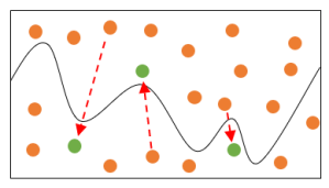
Figure 2: The solid line is model decision boundary. Orange circles refer to the unlabeled data and green circles refer to the corresponding augmentation of the orange unlabeled data.

The divergence objective exploits unlabeled data by measuring predictions across slightly-distorted versions of each unlabeled sample. The diverse and adversarial augmentations capture the local sensitivity and informativeness of inputs and project examples to the decision boundary Ducoffe and Precioso (2018). Thus, the examples and their copies with highly inconsistent model predictions lie close to the decision boundary of the model Gao et al. (2020). These examples are valuable to have human annotations because they 1) contain high-confidence region in a local perturbation and are therefore easy to train 2) are highly likely to promote the model with large-margin improvements (see example in Figure 2). Under our local sensitivity and hardness guided acquisition, we argue the selected examples would not be necessarily the examples with the highest uncertainty, which do not always benefit the training. For instance, an example may have low-confidence prediction of both original inputs and augmented inputs thus making the samples most hard to train.

2.4 More Details

Compute Distance We compute the divergence in the model predictive probabilities for the pairs of the input and its augmentations in Eqn (1). Specifically, we use a pretrained BERT in classification tasks and GPT-2 in prompt-based few-shot learning as the base model $p_{\theta}$ to obtain the output probabilities for all unlabeled data points in $\mathcal{D}_{pool}$. We then compute the divergence value with Eqn (1). Rank and Select Candidates We apply these steps to all candidate examples from $\mathcal{D}_{pool}$ and obtain the divergence value for each. Our acquisition function selects the top $s_{\textit{acq}}$ examples that have the highest divergence value from the acquired batch $\mathcal{T}$.

1:  Input: labeled data $\mathcal{D}_{label}$, unlabeled data $\mathcal{D}_{pool}$, acquisition size $s_{\textit{acq}}$, model $\mathcal{M}$ with output probability $p_{\theta}(\cdot\mid\boldsymbol{x})$.

2:  while  Select examples before reaching the budget  do

3:  for $\boldsymbol{x}$ in $\mathcal{D}_{pool}$ do

4:     Generate $K$ augmentations, $\left\{\boldsymbol{x}_{i}^{\prime}\right\}_{i=1,\cdots,K}\leftarrow g\left(\boldsymbol{x}\right)$.        //data paraphrasing via augmentation

5:     Compute $p_{\theta}(\cdot\mid\boldsymbol{x})$ and $p_{\theta}(\cdot\mid\boldsymbol{x}^{\prime}_{i})$ for $i=1,\ldots,K$.        //compute probabilities

6:     Select the worst case augmentation $\boldsymbol{x}^{\prime}$ for each input $\boldsymbol{x}$ as $\ell^{\textit{max}}(\boldsymbol{x})=\max_{i=1,\cdots,K}\ell(\boldsymbol{x},\boldsymbol{x}_{i}^{\prime})$.

7:  end for

8:  Select top $s_{\textit{acq}}$ largest examples in $\mathcal{D}_{pool}$, according to the value of $\mathbb{D}(p_{\theta}(\cdot\mid\boldsymbol{x}),p_{\theta}(\cdot\mid\boldsymbol{x^{\prime}}))$.

9:  Label these $s_{\textit{acq}}$ examples.

10:  end while

11:  Curriculum learning the model parameters with Eqn (5).

Algorithm 1 Acquisition with Local Sensitivity and Hardness

3 Experimental Settings

Table 1 shows the experimental data configuration. In classification tasks, we use five datasets, including Stanford Sentiment Treebank (SST-2; Socher et al. (2013)), Internet Movie Database (IMDB; Maas et al. (2011)), AG’s News Corpus (AG News; Zhang et al. (2015)), Quora Question Pairs (QQP; Wang et al. (2018a)), and Question NLI (QNLI; Wang et al. (2018a)). The validation and test splits are provided in Margatina et al. (2021). Following Desai and Durrett (2020), we test domain generalization and robustness on three challenging out-of-domain (OD) datasets. For sentiment analysis, SST-2 and IMDB are the source and target domains, respectively, and vice versa; for paraphrase detection, TwitterPPDB Lan et al. (2019) serves as the out-of-domain test dataset for QQP.

Dataset	Train	Val	Test	OD Dataset
SST-2	60.6K	6.7K	871	IMDB
IMDB	22.5K	2.5K	25K	SST-2
AG News	11.4K	6K	7.6K	-
QNLI	99.5K	5.2K	5.5K	-
QQP	327K	36.4K	80.8K	TwitterPPDB
SST-2	60.6K	6.7K	871	-
TREC	4.5K	500	500	-
RTE	2.5K	277	3K	-

Table 1: Dataset Configuration. The top block is for the classification tasks and the bottom block is for the prompt-based few-shot learning. OD represents out-of-domain datasets.

In the prompt-based few-shot learning, we follow Zhao et al. (2021) to use SST-2 Socher et al. (2013) for sentiment analysis, TREC Voorhees and Tice (2000) for question classification, and RTE Dagan et al. (2005) for recognizing textual entailment. See Appendix A for more details of the data.

3.1 Classification Task

We compare the proposed ALLSH  against four baseline methods. We choose these baselines as they cover a spectrum of acquisition functions (uncertainty, batch-mode, and diversity-based).

Random samples data from the pool of unlabeled data $\mathcal{D}_{pool}$ following a uniform distribution.

Entropy selects $s_{\textit{acq}}$ sentences with the highest predictive entropy Lewis and Gale (1994) measured by $-\sum\limits_{\boldsymbol{x}}p_{\theta}(\boldsymbol{x})\ln p_{\theta}(\boldsymbol{x}).$

BADGE Ash et al. (2020) acquires $s_{\textit{acq}}$ sentences based on diversity in loss gradient. The goal of BADGE is to sample a diverse and uncertain batch of points for training neural networks. It acquires data from $\mathcal{D}_{pool}$ by first passing the input through the trained model and computing the gradient embedding with respect to the parameters of the model’s last layer.

CAL Margatina et al. (2021) The acquisition function samples contrastive examples. It uses information from the feature space to create neighborhoods for unlabeled examples, and uses predictive likelihood for ranking the candidates.

3.2 Prompt-based Few-Shot Learning

Following Zhao et al. (2021), we adapt our acquisition function for state-of-the-art generation based model GPT-2 and propose to retrieve examples that are semantics and sensitivity aware to formulate its corresponding prompts. We compare ALLSH’s acquisition function with random, contextual calibrated, and uncertainty prompt. For random prompt, we randomly select in-context examples from the training set for each test sentence. For Calibrated, Zhao et al. (2021) inject calibration parameters that cause the prediction for each test input to be uniform across answers. See Zhao et al. (2021) for more details. For Uncertain, we sample the highest uncertain prompt for the test sentences. For ALLSH, we augment the in-context examples and select the prompts with the highest divergence of the predicted likelihood between the original examples and their augmentations.

3.3 Implementation Details

For classification, we use BERT-base Devlin et al. (2018) from the HuggingFace library Wolf et al. (2020). We train all models with batch size $16$, learning rate $2\times 10^{-5}$, and AdamW optimizer with epsilon $1\times 10^{-8}$. For all datasets, we set the default annotation budget as $1\%$, the maximum annotation budget as $15\%$, initial accumulated labeled data set $\mathcal{D}_{label}$ as $0.1\%$ of the whole unlabeled data, and acquisition size as $50$ instances for each active learning iterations, following prior work ($e.g.$, Gissin and Shalev-Shwartz, 2019; Dor et al., 2020; Ru et al., 2020). Curriculum Learning (CL) We further combine our acquisition function with advances in semi-supervised learning (SSL) Berthelot et al. (2019a); Sohn et al. (2020), which also integrates abundant unlabeled data into learning. A recent line of work in SSL utilizes data augmentations, such as TF-IDF and back-translation, to enforce local consistency of the model (Sajjadi et al., 2016; Miyato et al., 2018). Here SSL can further distill information from unlabeled data and gradually propagate label information from labeled examples to unlabeled one during the training stage Xie et al. (2020); Zhang et al. (2021c). We construct the overall loss function as

$$\leavevmode\resizebox{375.80542pt}{}{$\mathcal{L}=\mathcal{L}_{S}+\alpha\cdot\underbrace{\mathbb{E}_{\boldsymbol{x}\sim\mathcal{D}_{pool}}\mathbb{D}(p_{\theta}(\cdot\mid\boldsymbol{x}),p_{\theta}(\cdot\mid\boldsymbol{x}^{\prime}))}_{\mathcal{L}_{U}}$},$$ (5)

where $\mathcal{L}_{S}$ is the cross-entropy supervised learning loss over labeled samples, $\mathcal{L}_{U}$ is the consistency regularization term, and $\alpha$ is a coefficient Tarvainen and Valpola (2017); Berthelot et al. (2019b).

For prompt-based few-shot learning, we run experiments on 1.5B-parameters GPT-2 Radford et al. (2019), a Transformer Vaswani et al. (2017) based language model. It largely follows the details of the OpenAI GPT model Radford et al. (2018). We take the TF-IDF as the default augmentation method and provide a rich analysis of other augmentation methods in Section 5. More detailed experimental settings are included in Appendix A.

4 Experiments

We evaluate the performance of our acquisition and learning framework in this section. We bold the best results within Random, Entropy, BADGE, CAL, and the proposed ALLSH (Ours) in tables. Then, we bold the best result within each column block. All experimental results are obtained with five independent runs to determine the variance. See Appendix A for the full results with error bars.

4.1 In-Domain Classification Task Results

In Table 2, we evaluate the impact of our acquisition function under three different annotation budgets ($1\%$, $5\%$, and $10\%$). With a constrained annotation budget, we see substantial gains on test accuracy with our proposed acquisition: ALLSH and selecting worst-case augmentation. With this encouraging initial results, we further explore our acquisition with curriculum learning. Across all settings, ALLSH is consistently the top performing method especially in SST-2, IMDB, and AG News. With a tight budget, our proposed acquisition can successfully integrate the local sensitivity and learning difficulty to generate annotated data.

For BADGE, despite combining both uncertainty and diversity sampling, it only achieves the comparable results on QNLI, showing that gradient computing may not directly benefit data acquisitions. In addition, requiring clustering for high dimensional data, BADGE is computationally heavy as its complexity grows exponentially with the acquisition size Yuan et al. (2020). We provide rich analysis of the sampling efficiency and running time for each method in Appendix A and include the results in Table 13. Also, ALLSH  outperforms the common uncertainty sampling in most cases. Given the current model state, uncertainty sampling chooses the samples that are not representative to the whole unlabeled data, leading to ineffective sampling. CAL has an effective contrastive acquiring on QNLI. We hypothesize that due to the presence of lexical and syntactic ambiguity between a pair of sentence, the contrastive examples can be used to push away the inputs in the feature space.

	Acquired dataset size:	1%	5%	10%
SST-2	Random	84.11	86.53	88.05
	Entropy	84.53	87.82	89.45
	BADGE	84.32	87.11	88.72
	CAL	84.95	87.34	89.16
	Ours	85.97	88.61	90.05
	+ WCA	86.12	88.56	90.14
	+ CL	86.37	88.79	90.18
IMDB	Random	65.90	84.22	86.25
	Entropy	68.32	84.51	87.29
	BADGE	67.80	84.46	87.17
	CAL	73.55	84.72	87.27
	Ours:	75.23	85.82	87.91
	+ WCA	75.17	85.79	87.83
	+ CL	77.57	86.02	88.43
AG News	Random	85.43	90.05	91.93
	Entropy	86.48	92.21	92.65
	BADGE	86.81	90.72	92.41
	CAL	87.12	92.13	92.82
	Ours	88.42	92.86	93.13
	+ WCA	88.50	92.84	93.22
	+ CL	88.57	92.94	93.20
QNLI	Random	76.33	83.61	84.63
	Entropy	77.95	83.83	84.75
	BADGE	77.74	84.90	84.32
	CAL	78.53	85.14	84.99
	Ours	78.44	84.93	84.87
	+ WCA	78.47	85.12	84.91
	+ CL	78.92	85.06	84.96
QQP	Random	77.32	81.73	84.22
	Entropy	78.47	81.92	86.03
	BADGE	78.02	81.63	84.06
	CAL	78.23	82.52	84.25
	Ours	78.97	82.43	84.77
	+ WCA	78.90	82.55	84.83
	+ CL	79.32	82.91	84.95

Table 2: Results of the in-domain test accuracies for different acquired dataset size. $+$ WCA refers to Ours $+$ select worst-case augmentation. $+$ CL refers to Ours $+$ curriculum learning. We provide error bars in Table 11 in the Appendix.

4.2 Out-of-Domain Classification Task Results

We compare our proposed method with the baselines for their performance in an out-of-domain (OD) setting and summarize the results in Table 3. We test domain generalization on three datasets with two tasks, including sentiment analysis and paraphrase detection. We set the annotation budget as $15\%$ of $\mathcal{D}_{pool}$ for all OD experiments. For OD in SST-2 and IMDB, ALLSH yields better results than all baselines with a clear margin ($1.7\%$ and $2.0\%$, respectively). With curriculum learning, the results are continually improved. The performance gains on out-of-domain are often greater than the gains on in-domain, implying that ALLSH can significantly help the model to generalize across domains. On QQP, ALLSH achieves comparable results as CAL without curriculum learning while the performance can be further improved by adding curriculum learning.

ID	SST-2	IMDB	QQP
OD	IMDB	SST-2	TwitterPPDB
Random	76.31	82.01	85.57
Entropy	75.88	85.32	85.18
BADGE	75.23	85.11	85.39
CAL	78.88	84.92	86.14
Ours	80.54	86.97	86.03
+ WCA	80.72	86.99	86.07
+ CL	80.91	87.07	86.18

Table 3: Results of out-of-domain (OD) generalization. We report the out-of-domain accuracy on the target domain. ID refers to in-domain dataset. OD refers to out-of-domain dataset.

4.3 Prompt-Based Few-Shot Learning Results

We present the prompt-based few-shot learning results with GPT-2 in Table 4, in which we follow the setting (4-shot, 8-shot, and 12-shot) in Zhao et al. (2021). Few-shot learners suffer from the quality of labeled data (Sohn et al., 2020), and previous acquisition functions usually fail to boost the performance from labeling random sampled data. In Table 4, we observe that uncertain prompts performs similar to random selected prompts. A potential reason is that an under-trained model treats all examples as uncertainty examples and hard to distinguish the informativeness. However, our proposed acquisition demonstrates the strong capability in modeling the local sensitivity and learning from easy to hard. It comes to the best performance in most of the settings. These findings show the potential of using our acquisition to improve prompt-based few-shot learning and make a good in-context examples for GPT-2 model.

		4-shot	8-shot	12-shot
SST-2	Random	64.9	54.5	56.3
	Calibrated	73.8	64.6	73.0
	Uncertainty	59.7	64.5	66.8
	Ours	75.3	77.8	79.7
TREC	Random	23.1	32.7	37.5
	Calibrated	44.2	44.1	44.4
	Uncertainty	34.8	52.2	54.1
	Ours	46.4	58.7	59.8
RTE	Random	53.2	54.9	56.0
	Calibrated	57.5	57.7	58.2
	Uncertainty	57.0	57.3	57.8
	Ours	57.9	58.4	59.7

Table 4: Results across different strategies of acquiring training examples (the prompt format is fixed). The language model here is GPT-2 (1.5B).

5 Analysis

Can we use our proposed acquisition in the imbalance setting?

Extreme label imbalance is an important challenge in many non-pairwise NLP tasks Sun et al. (2009); Zhang et al. (2017); Mussmann et al. (2020b). We set up the imbalance setting by sampling a subset with class-imbalance sample rate. For binary classification, we set the positive-class data sample rate as $1.0$ and negative-class data sample rate as $0.1$. As our acquisition focuses on local sensitivity and informativeness, it tends to select examples close to the decision boundary. Once too many positive examples and few negative examples are labeled, the local perturbation around negative samples are easy to be positive, and thus ALLSH selects examples that are close to the negative examples. We conduct the experiments on SST-2, IMDB, and AG News with annotation budget as $1\%$. In Table 5, Ours indicates strong improvements. This further proves that our selection method can generalize better.

	SST-2	IMDB	AG News
Random	79.45	62.33	82.95
Entropy	81.71	65.69	82.79
CAL	83.23	72.75	83.27
Ours	85.48	74.48	84.11

Table 5: Main results of different active learning strategies on the imbalanced SST-2, IMDB, and AG News.

Would different augmentations make meaningful difference?

We test if our results are sensitive to the choice of augmentation: TF-IDF and backtranslation. For TF-IDF, we compare the random sample augmentation and worst-case augmentation (WCA). TF-IDF and Backtranslation generate diverse paraphrases while preserving the semantics of the original sentences. Select-worst case augments the inputs by incorporating the approximate adversarial perturbations. Table 6 indicates our method is insensitive to different augmentations. We also observe that WCA achieves the highest gains on two datasets. This confirms our discussion in Section 2.3 that select-worst case is capable of imposing local sensitivity.

	SST-2	IMDB	AG News
Backtranslation	86.01	75.12	88.39
TF-IDF	85.97	75.23	88.42
+ WCA	86.37	75.17	88.50

Table 6: Acquisition performance for different augmentations. We report results of our acquisition with different augmentations to get the local copies of the samples.

What is the influence of the choice of divergence?

We select different divergences in the statistical distance family and study their abilities in encoding different information. Corresponding to Section 2.3, we present the results in Table 7. We experiment on the KL divergence, JSD, and $\alpha$-divergence Minka et al. (2005) with the $\alpha$ value set as $-0.5$ or $0.5$. We notice that for our case the difference between different divergences is small. A possible reason is that the number of class categories is small and therefore the choice of divergence does not have a large influence.

Can we use the proposed acquisition with extremely few labeled data?

We have presented the results under very limited annotation budgets in Table 2. We set the annotation budget as $0.8\%$ and $0.4\%$. The key observation is that the degradation of performance in the other acquisition functions are dramatic. For example, in IMDB, the uncertainty sampling (Entropy) shows the obvious performance drop. It suffers from the sampling bias problem because of the frequent variation of the decision boundary in the early phase of training with very few labeled data available, which results in ineffective sampling. Even under this extreme case, our acquisition still aims to select the most informative examples for the model. This further verifies our empirical results in Section 4.3 on prompt-based few-shot learning where only a very few in-context prompts are provided.

6 Related Work

Active Learning

Active Learning has been widely used in many applications in NLP Lowell et al. (2018); Dor et al. (2020); Ru et al. (2020). The uncertainty-based methods Fletcher et al. (2008)

	SST-2	IMDB	AG News
KL	86.37	77.57	88.57
JSD	86.25	77.38	88.41
$\alpha=-0.5$	86.31	77.42	88.43
$\alpha=0.5$	86.39	77.53	88.61

Table 7: Ablation study on different choices of divergences. We report KL, JSD, and $\alpha$-divergence, and set $\alpha=\pm 0.5$ respectively.

	SST-2			IMDB
Dataset size	0.4%	0.8%		0.4%	0.8%
Random	64.64	61.08		60.84	73.86
Entropy	67.88	63.94		58.96	71.32
CAL	73.81	65.72		61.65	74.15
Ours	76.45	69.46		64.54	75.88

Table 8: Results on the SST-2 and IMDB datasets under limited annotation budget (0.4%, 0.8%).

have become the most common strategy. Instead of only considering uncertainty, diversity sampling has also become an alternative direction. Recent works Geifman and El-Yaniv (2017); Sener and Savarese (2017); Ash et al. (2020); Yuan et al. (2020) focus on different parts of diversity. Most recent works ($e.g.$ Zhang and Plank, 2021; Margatina et al., 2021) have been more on exploiting the model behavior and each individual instance. Our work focuses more on the local sensitivity and informativeness of data, leading to better performance under various limited annotation settings.

Annotation Budgeting

Annotation budgeting with learning has long been studied Turney (2002). Sheng et al. (2008) study the tradeoff between collecting multiple labels per example versus annotating more examples. On the other hand, different labeling strategies such as providing fine-grained rationales Dua et al. (2020), active learning Kirsch et al. (2019), and the training dynamics approach  Swayamdipta et al. (2020) are studied. Except standard classification, class-imbalance Mussmann et al. (2020a) or noisy label cases Fan et al. (2021); Chen et al. (2021) have also been explored. We utilize active learning to explore the labeling strategies and aim to select the most informative data for annotations.

7 Conclusion

Our work demonstrates the benefits of introducing local sensitivity and learning from easy to hard into the acquisition strategy. The proposed acquisition function shows noticeable gains in performance across classification tasks and prompt-based few-shot learning. In this work, we conduct the detailed study with the proposed acquisition strategy in different settings, including imbalanced and extremely limited labels. We also verify the impact of different choice of designs such as the choice of divergence and augmentations. To summarize, the proposed ALLSH is effective and general, with the potential to be incorporated into existing models for various NLP tasks.

Appendix A Experimental details

A.1 Full Results and Examples

We report the full results of out-of-domain and in-domain tasks in Tables 9 and 11, respectively. The full results of prompt-based few-shot learning are shown in Table 10 and Table 12 shows prompt examples of each task.

ID	SST-2	IMDB	QQP
OD	IMDB	SST-2	TwitterPPDB
Random	76.31$\pm$0.66	82.01$\pm$3.45	85.57$\pm$0.42
Entropy	75.88$\pm$1.82	85.32$\pm$2.36	85.18$\pm$1.79
BADGE	75.23$\pm$0.87	85.11$\pm$2.92	85.39$\pm$3.44
CAL	78.88$\pm$1.27	84.92$\pm$2.30	86.14$\pm$0.31
Ours	80.24$\pm$0.91	86.07$\pm$2.45	86.03$\pm$0.40
+ WCA	80.42$\pm$0.85	86.19$\pm$2.37	86.07$\pm$0.36
+ CL	80.51$\pm$0.67	86.24$\pm$1.98	86.18$\pm$0.29

Table 9: Results of out-of-domain (OD) generalization. We report the out-of-domain accuracy on the target domain. ID refers to in-domain dataset. OD refers to out-of-domain dataset.

		4-shot	8-shot	12-shot
SST-2	Random	64.9$\pm$8.4	54.5$\pm$4.6	56.3$\pm$2.3
	Calibrated	73.8$\pm$10.9	64.6$\pm$8.8	73.0 $\pm$5.3
	Uncertainty	59.7$\pm$7.3	64.5$\pm$5.9	66.8$\pm$4.8
	Ours	75.3$\pm$7.8	77.8$\pm$4.7	79.7$\pm$3.2
TREC	Random	23.1$\pm$5.9	32.7$\pm$7.5	37.5$\pm$7.8
	Calibrated	44.2$\pm$2.2	44.1$\pm$3.6	44.4$\pm$4.0
	Uncertainty	34.8$\pm$3.4	52.2$\pm$4.1	54.1$\pm$5.2
	Ours	46.4$\pm$2.8	58.7$\pm$3.6	59.8$\pm$4.3
RTE	Random	53.2$\pm$6.0	54.9$\pm$3.0	56.0$\pm$2.2
	Calibrated	57.5$\pm$1.8	57.7$\pm$1.3	58.2$\pm$1.1
	Uncertainty	57.0$\pm$1.5	57.3$\pm$1.4	57.8$\pm$1.1
	Ours	57.9$\pm$2.3	58.4$\pm$1.6	59.7$\pm$1.2

Table 10: Full results across different choices of the training examples (the prompt format is fixed). The language model at here is GPT-2XL (1.5B).

	Acquired dataset size:	1%	5%	10%
SST-2	Random	84.11$\pm$0.45	86.53$\pm$0.61	88.05$\pm$0.73
	Entropy	84.53$\pm$0.81	87.82$\pm$0.73	89.45$\pm$0.92
	BADGE	84.32$\pm$0.64	87.11$\pm$0.82	88.72$\pm$0.44
	CAL	84.95$\pm$0.56	87.34$\pm$0.61	89.16$\pm$0.67
	Ours	85.97$\pm$0.53	88.61$\pm$0.48	90.05$\pm$0.61
	+ WCA	86.12$\pm$0.47	88.56$\pm$0.55	90.14$\pm$0.57
	+ CL	86.37$\pm$0.43	88.79$\pm$0.46	90.18$\pm$0.48
IMDB	Random	65.96$\pm$0.66	84.22$\pm$0.52	86.25$\pm$0.54
	Entropy	68.32$\pm$0.53	84.51$\pm$0.48	87.29$\pm$0.51
	BADGE	67.80$\pm$0.44	84.46$\pm$0.50	87.17$\pm$0.41
	CAL	73.55$\pm$0.56	84.72$\pm$0.48	87.27$\pm$0.50
	Ours:	75.23$\pm$0.43	85.82$\pm$0.35	87.91$\pm$0.53
	+ WCA	75.17$\pm$0.58	85.79$\pm$0.67	87.83$\pm$0.71
	+ CL	77.57$\pm$0.64	86.02$\pm$0.62	88.43$\pm$0.57
AG News	Random	85.43$\pm$0.53	90.05$\pm$0.51	91.93$\pm$0.60
	Entropy	86.48$\pm$0.46	92.21$\pm$0.41	92.65$\pm$0.39
	BADGE	86.81$\pm$0.48	90.72$\pm$0.51	92.41$\pm$0.53
	CAL	87.12$\pm$0.31	92.13$\pm$0.38	92.82$\pm$0.35
	Ours	88.42$\pm$0.37	92.86$\pm$0.40	93.13$\pm$0.39
	+ WCA	88.50$\pm$0.35	92.84$\pm$0.37	93.22$\pm$0.42
	+ CL	88.57$\pm$0.30	92.94$\pm$0.32	93.20$\pm$0.35
QNLI	Random	76.33$\pm$0.54	83.61$\pm$0.57	84.63$\pm$0.62
	Entropy	77.95$\pm$0.50	83.83$\pm$0.61	84.75$\pm$0.55
	BADGE	77.74$\pm$0.53	84.90$\pm$0.48	84.32$\pm$0.46
	CAL	78.53$\pm$0.49	85.14$\pm$0.45	84.99$\pm$0.53
	Ours	78.44$\pm$0.41	84.93$\pm$0.32	84.87$\pm$0.39
	+ WCA	78.47$\pm$0.43	85.12$\pm$0.37	84.91$\pm$0.38
	+ CL	78.92$\pm$s0.40	85.06$\pm$0.36	84.96$\pm$0.33
QQP	Random	77.32$\pm$0.66	81.73$\pm$0.72	84.22$\pm$0.75
	Entropy	78.47$\pm$0.57	81.92$\pm$0.64	86.03$\pm$0.49
	BADGE	78.02$\pm$0.49	81.63$\pm$0.55	84.06$\pm$0.60
	CAL	78.23$\pm$0.52	82.52$\pm$0.57	84.25$\pm$0.48
	Ours	78.97$\pm$0.46	82.43$\pm$0.44	84.77$\pm$0.52
	+ WCA	78.90$\pm$0.50	82.55$\pm$0.48	84.83$\pm$0.48
	+ CL	79.32$\pm$0.53	82.91$\pm$0.51	84.95$\pm$0.58

Table 11: Full results of the in-domain test accuracies for different acquired dataset size. $+$ WCA refers to Ours $+$ select worst-case augmentation. $+$ CL refers to Ours $+$ curriculum learning.

Task	Prompt	Label Names
SST-2	Review: At times, the movie looks genuinely pretty.	Positive, Negative
	Sentiment: Positive
	Review: The movie is amateurish, but it’s a minor treat.
	Sentiment:
TREC	Question: Where can I find information on becoming a journalist?	Number, Location, Person, Description,
	Answer Type: Location	Entity, Abbreviation
	Question: What is the temperature today?
	Answer Type:
RTE	The motor industry accounts for as much as 40 percent of the 450,000 installed industrial robots	True, False
	worldwide but their use is changing and applications are expanding.
	Question: The most common use for robots is the manufacture of automobiles. True or False?
	Answer: True
	Arroyo was the favorite of investors because of her experience as a trained economist
	and government manager.
	Question: Arroyo has experience as an economist and as a government manager. True or False?
	Answer:

Table 12: The different prompts we use for SST-2, TREC, and RTE. One training example per task is presented. The language model is used to predicted the label probability as shown in the right column.

A.2 Classification Task Hyperparameters and Experimental Settings

Our implementation is based on the BERT-base Devlin et al. (2018) from HuggingFace Transformers (Wolf et al., 2020). We optimize the KL divergence as the objective with the Adam optimizer (Kingma and Ba, 2014) and batch size is set to 16 for all experiments. The curriculum learning is trained for $200$ iterations. The learning rate is $2\times 10^{-5}$. The $\alpha$ in Eqn (5) is set as $0.01$ for all experiments. With longer input texts such as IMDB, we use $256$ as the maximum sequence length. For others, we use $128$. Following Ash et al. (2020) and Margatina et al. (2021), for the initial training set $\mathcal{D}_{label}$, we begin the active learning loop by uniformly random sampling from $\mathcal{D}_{pool}$. For all experiments in the Section 5, we set the annotation budget as $1\%$ and use Ours (ours + curriculum learning) as the default methods.

TF-IDF based data augmentation Xie et al. (2020) aims to generate both diverse and valid examples. It is designed to retain keywords and replace uninformative words with other uninformative words. BERT is used as the word tokenizer. We set IDF$(w)$ is the IDF score for word $w$ computed on the whole corpus, and TF$(w)$ is the TF score for word $w$ in a sentence. Then, we compute the TF-IDF score as TFIDF$(w)=$ TF$(w)$IDF$(w)$. Suppose the maximum TF-IDF score in a sentence $\boldsymbol{x}$ is C = max_i TFIDF$(x_{i})$. We set the probability to min($p$(C - TFIDF$(x_{i})$)/Z, 1), where $p$ is a hyperparameter that controls the magnitude of the augmentation and we set $p=$0.3. Z is the average score over the inputs sentence. For backtranslation, we use a pre-trained EN-DE and DE-EN translation models Ng et al. (2019) to perform backtranslation on each sentence.

A.3 Prompt-based Few-Shot Learning Hyperparameters and Experimental Settings

We use the 1.5B parameters GPT-2 Radford et al. (2019), with a Transformer Vaswani et al. (2017) based architecture. The model largely follows the details of the OpenAI GPT model Radford et al. (2018) with a few modifications. Layer normalization Ba et al. (2016); Fan et al. (2020); Zhang et al. (2021a) is moved to the input of each sub-block and an additional layer normalization is added after the final self-attention block. Following the settings in Zhao et al. (2021), the maximum input length is 2048 tokens or 1500 words. In Table 12, we show the default prompt format for SST-2, TREC, and RTE. For datasets, Stanford Sentiment Treebank (SST-2) Socher et al. (2013) is one of benchmarks in General Language Understanding Evaluation (GLUE) Wang et al. (2018a). With fully labeled parse tress, This corpus allows a complete analysis of the compositional effects of sentiment in language. TREC Voorhees and Tice (2000) is a 6-way question classification. The target is to classify the questions based on whether their answer type is a Number, Location, Person, Description, Entity, or Abbreviation. Similarly, RTE (Recognizing Textual Entailment) Dagan et al. (2005) is also a benchmark dataset from GLUE. It is a binary classification task to determine if a given premise entails a given hypothesis.

A.4 Sampling Efficiency and Running Time

	SST-2	IMDB	AG News	AVG.
Random	0	0	0	0
Entropy	173	107	402	227
BADGE	25640	3816	1961	10303
CAL	708	273	1284	755
Ours	513	228	881	541
+ WCA	611	275	1023	636

Table 13: Running time (seconds) per sampling iteration (inference and selection) during AL acquisition for each datasets. AVG. refers the average acquisition time for all three datasets. For each acquisition, we report the running time under three adversarial attacks respectively

We mask $m$ as the number of labeled data in $\mathcal{D}_{label}$, $n$ the number of unlabeled data in $\mathcal{D}_{pool}$, $C$ the number of classes in the downstream classification task, $d$ the dimension of embeddings, $l$ the maximum sequence length, and $s_{\textit{acq}}$ the acquisition size. We set these values following Yuan et al. (2020) and Margatina et al. (2021). In Table 13, running time in seconds are summarized per sampling iteration (inference and selection) during AL acquisition for each dataset. Experiments in this part are performed on a Tesla V100 GPU. We keep $s_{\textit{acq}}=100,d=768,t=10$, and $l=128$. For IMDB, we change the maximum sequence length to $256$. As demonstrated in Table 13, BADGE requires a significantly amount of running time, since it has to cluster high-dimensional vectors and is a very computationally-heavy method. CAL also requires relative long running time as it needs to find the contrastive examples by finding nearest neighbors and computing contrastive score for unlabeled candidates. Our method achieves the second best efficiency. Even with the select worst-case augmentation, our acquisition function is still computationally productive as the augmentation and ranking candidates can be well deployed in the current computational machines. Entropy is overall the most efficient method as it only requires to rank the list of uncertainty scores, while it tends to have weaker performance.

References

- Ash et al. (2020) Jordan T. Ash, Chicheng Zhang, Akshay Krishnamurthy, John Langford, and Alekh Agarwal. 2020. Deep batch active learning by diverse, uncertain gradient lower bounds. In International Conference on Learning Representations.
- Ba et al. (2016) Jimmy Lei Ba, Jamie Ryan Kiros, and Geoffrey E Hinton. 2016. Layer normalization. arXiv preprint arXiv:1607.06450.
- Bengio et al. (2009) Yoshua Bengio, Jérôme Louradour, Ronan Collobert, and Jason Weston. 2009. Curriculum learning. In Proceedings of the 26th annual international conference on machine learning, pages 41–48.
- Berthelot et al. (2019a) David Berthelot, Nicholas Carlini, Ekin D Cubuk, Alex Kurakin, Kihyuk Sohn, Han Zhang, and Colin Raffel. 2019a. Remixmatch: Semi-supervised learning with distribution alignment and augmentation anchoring. arXiv preprint arXiv:1911.09785.
- Berthelot et al. (2019b) David Berthelot, Nicholas Carlini, Ian Goodfellow, Nicolas Papernot, Avital Oliver, and Colin Raffel. 2019b. Mixmatch: A holistic approach to semi-supervised learning. arXiv preprint arXiv:1905.02249.
- Blum and Chawla (2001) Avrim Blum and Shuchi Chawla. 2001. Learning from labeled and unlabeled data using graph mincuts.
- Bodó et al. (2011) Zalán Bodó, Zsolt Minier, and Lehel Csató. 2011. Active learning with clustering. In Active Learning and Experimental Design workshop In conjunction with AISTATS 2010, pages 127–139. JMLR Workshop and Conference Proceedings.
- Bowman et al. (2015) Samuel R. Bowman, Gabor Angeli, Christopher Potts, and Christopher D. Manning. 2015. A large annotated corpus for learning natural language inference. Proceedings of the Conference on Empirical Methods in Natural Language Processing (EMNLP), abs/1508.05326.
- Chapelle et al. (2009) Olivier Chapelle, Bernhard Scholkopf, and Alexander Zien. 2009. Semi-supervised learning (chapelle, o. et al., eds.; 2006)[book reviews]. IEEE Transactions on Neural Networks, 20(3):542–542.
- Chapelle et al. (2002) Olivier Chapelle, Jason Weston, and Bernhard Schölkopf. 2002. Cluster kernels for semi-supervised learning. In Advances in neural information processing systems. Citeseer.
- Chen et al. (2021) Derek Chen, Zhou Yu, and Samuel R Bowman. 2021. Learning with noisy labels by targeted relabeling. arXiv preprint arXiv:2110.08355.
- Culotta and McCallum (2005) Aron Culotta and Andrew McCallum. 2005. Reducing labeling effort for structured prediction tasks. In AAAI, volume 5, pages 746–751.
- Dagan et al. (2005) Ido Dagan, Oren Glickman, and Bernardo Magnini. 2005. The pascal recognising textual entailment challenge. In Machine Learning Challenges Workshop, pages 177–190. Springer.
- Desai and Durrett (2020) Shrey Desai and Greg Durrett. 2020. Calibration of pre-trained transformers. Conference on Empirical Methods in Natural Language Processing, abs/2003.07892.
- Devlin et al. (2018) Jacob Devlin, Ming-Wei Chang, Kenton Lee, and Kristina Toutanova. 2018. Bert: pre-training of deep bidirectional transformers for language understanding. arxiv. arXiv preprint arXiv:1810.04805.
- Dor et al. (2020) Liat Ein Dor, Alon Halfon, Ariel Gera, Eyal Shnarch, Lena Dankin, Leshem Choshen, Marina Danilevsky, Ranit Aharonov, Yoav Katz, and Noam Slonim. 2020. Active learning for bert: An empirical study. In Proceedings of the 2020 Conference on Empirical Methods in Natural Language Processing (EMNLP), pages 7949–7962.
- Dua et al. (2020) Dheeru Dua, Sameer Singh, and Matt Gardner. 2020. Benefits of intermediate annotations in reading comprehension. In Proceedings of the Annual Meeting of the Association for Computational Linguistics (ACL).
- Ducoffe and Precioso (2018) Melanie Ducoffe and Frederic Precioso. 2018. Adversarial active learning for deep networks: a margin based approach. arXiv preprint arXiv:1802.09841.
- Edunov et al. (2018) Sergey Edunov, Myle Ott, Michael Auli, and David Grangier. 2018. Understanding back-translation at scale. arXiv preprint arXiv:1808.09381.
- Endres and Schindelin (2003) Dominik Maria Endres and Johannes E Schindelin. 2003. A new metric for probability distributions. IEEE Transactions on Information theory, 49(7):1858–1860.
- Fan et al. (2020) Xinjie Fan, Shujian Zhang, Bo Chen, and Mingyuan Zhou. 2020. Bayesian attention modules. arXiv preprint arXiv:2010.10604.
- Fan et al. (2021) Xinjie Fan, Shujian Zhang, Korawat Tanwisuth, Xiaoning Qian, and Mingyuan Zhou. 2021. Contextual dropout: An efficient sample-dependent dropout module. arXiv preprint arXiv:2103.04181.
- Fazlyab et al. (2019) Mahyar Fazlyab, Alexander Robey, Hamed Hassani, Manfred Morari, and George J Pappas. 2019. Efficient and accurate estimation of lipschitz constants for deep neural networks. arXiv preprint arXiv:1906.04893.
- Ferracane et al. (2021) Elisa Ferracane, Greg Durrett, Junyi Jessy Li, and Katrin Erk. 2021. Did they answer? subjective acts and intents in conversational discourse. In Proceedings of the 2021 Conference of the North American Chapter of the Association for Computational Linguistics: Human Language Technologies, pages 1626–1644, Online. Association for Computational Linguistics.
- Fletcher et al. (2008) Alyson K Fletcher, Sundeep Rangan, and Vivek K Goyal. 2008. Resolution limits of sparse coding in high dimensions. In NIPS, pages 449–456.
- Gao et al. (2020) Mingfei Gao, Zizhao Zhang, Guo Yu, Sercan Ö Arık, Larry S Davis, and Tomas Pfister. 2020. Consistency-based semi-supervised active learning: Towards minimizing labeling cost. In European Conference on Computer Vision, pages 510–526. Springer.
- Geifman and El-Yaniv (2017) Yonatan Geifman and Ran El-Yaniv. 2017. Deep active learning over the long tail. arXiv preprint arXiv:1711.00941.
- Gissin and Shalev-Shwartz (2019) Daniel Gissin and Shai Shalev-Shwartz. 2019. Discriminative active learning. arXiv preprint arXiv:1907.06347.
- Gong et al. (2020) Chengyue Gong, Tongzheng Ren, Mao Ye, and Qiang Liu. 2020. Maxup: A simple way to improve generalization of neural network training. arXiv preprint arXiv:2002.09024.
- Kingma and Ba (2014) Diederik P Kingma and Jimmy Ba. 2014. Adam: A method for stochastic optimization. arXiv preprint arXiv:1412.6980.
- Kirsch et al. (2019) Andreas Kirsch, Joost Van Amersfoort, and Yarin Gal. 2019. Batchbald: Efficient and diverse batch acquisition for deep bayesian active learning. Advances in neural information processing systems, 32:7026–7037.
- Kullback and Leibler (1951) Solomon Kullback and Richard A Leibler. 1951. On information and sufficiency. The annals of mathematical statistics, 22(1):79–86.
- Lan et al. (2019) Zhenzhong Lan, Mingda Chen, Sebastian Goodman, Kevin Gimpel, Piyush Sharma, and Radu Soricut. 2019. Albert: A lite bert for self-supervised learning of language representations. arXiv preprint arXiv:1909.11942.
- Lei et al. (2018) Qi Lei, Lingfei Wu, Pin-Yu Chen, Alexandros G Dimakis, Inderjit S Dhillon, and Michael Witbrock. 2018. Discrete adversarial attacks and submodular optimization with applications to text classification. arXiv preprint arXiv:1812.00151.
- Lewis and Gale (1994) David D Lewis and William A Gale. 1994. A sequential algorithm for training text classifiers. In SIGIR’94, pages 3–12. Springer.
- Lowell et al. (2018) David Lowell, Zachary C Lipton, and Byron C Wallace. 2018. Practical obstacles to deploying active learning. arXiv preprint arXiv:1807.04801.
- Maas et al. (2011) Andrew Maas, Raymond E Daly, Peter T Pham, Dan Huang, Andrew Y Ng, and Christopher Potts. 2011. Learning word vectors for sentiment analysis. In Proceedings of the 49th annual meeting of the association for computational linguistics: Human language technologies, pages 142–150.
- Madry et al. (2017) Aleksander Madry, Aleksandar Makelov, Ludwig Schmidt, Dimitris Tsipras, and Adrian Vladu. 2017. Towards deep learning models resistant to adversarial attacks. arXiv preprint arXiv:1706.06083.
- Margatina et al. (2021) Katerina Margatina, Giorgos Vernikos, Loïc Barrault, and Nikolaos Aletras. 2021. Active learning by acquiring contrastive examples. arXiv preprint arXiv:2109.03764.
- Minka et al. (2005) Tom Minka et al. 2005. Divergence measures and message passing. Technical report, Citeseer.
- Miyato et al. (2018) Takeru Miyato, Shin-ichi Maeda, Masanori Koyama, and Shin Ishii. 2018. Virtual adversarial training: a regularization method for supervised and semi-supervised learning. IEEE transactions on pattern analysis and machine intelligence, 41(8):1979–1993.
- Mussmann et al. (2020a) Stephen Mussmann, Robin Jia, and P. Liang. 2020a. On the importance of adaptive data collection for extremely imbalanced pairwise tasks. In Conference on Empirical Methods in Natural Language Processing.
- Mussmann et al. (2020b) Stephen Mussmann, Robin Jia, and Percy Liang. 2020b. On the importance of adaptive data collection for extremely imbalanced pairwise tasks. arXiv preprint arXiv:2010.05103.
- Ng et al. (2019) Nathan Ng, Kyra Yee, Alexei Baevski, Myle Ott, Michael Auli, and Sergey Edunov. 2019. Facebook fair’s wmt19 news translation task submission. arXiv preprint arXiv:1907.06616.
- Nie et al. (2020) Yixin Nie, Xiang Zhou, and Mohit Bansal. 2020. What can we learn from collective human opinions on natural language inference data? In Proceedings of the 2020 Conference on Empirical Methods in Natural Language Processing (EMNLP), pages 9131–9143.
- Pavlick and Kwiatkowski (2019) Ellie Pavlick and Tom Kwiatkowski. 2019. Inherent disagreements in human textual inferences. Transactions of the Association for Computational Linguistics, 7:677–694.
- Pillutla et al. (2021) Krishna Pillutla, Swabha Swayamdipta, Rowan Zellers, John Thickstun, Sean Welleck, Yejin Choi, and Zaid Harchaoui. 2021. Mauve: Measuring the gap between neural text and human text using divergence frontiers. Advances in Neural Information Processing Systems, 34.
- Radford et al. (2018) Alec Radford, Karthik Narasimhan, Tim Salimans, and Ilya Sutskever. 2018. Improving language understanding by generative pre-training.
- Radford et al. (2019) Alec Radford, Jeffrey Wu, Rewon Child, David Luan, Dario Amodei, Ilya Sutskever, et al. 2019. Language models are unsupervised multitask learners. OpenAI blog, 1(8):9.
- Rajpurkar et al. (2016) Pranav Rajpurkar, Jian Zhang, Konstantin Lopyrev, and Percy Liang. 2016. Squad: 100, 000+ questions for machine comprehension of text. In Proceedings of the Conference on Empirical Methods in Natural Language Processing (EMNLP).
- Ru et al. (2020) Dongyu Ru, Jiangtao Feng, Lin Qiu, Hao Zhou, Mingxuan Wang, Weinan Zhang, Yong Yu, and Lei Li. 2020. Active sentence learning by adversarial uncertainty sampling in discrete space. arXiv preprint arXiv:2004.08046.
- Sajjadi et al. (2016) Mehdi Sajjadi, Mehran Javanmardi, and Tolga Tasdizen. 2016. Regularization with stochastic transformations and perturbations for deep semi-supervised learning. Advances in neural information processing systems, 29:1163–1171.
- Scaman and Virmaux (2018) Kevin Scaman and Aladin Virmaux. 2018. Lipschitz regularity of deep neural networks: analysis and efficient estimation. arXiv preprint arXiv:1805.10965.
- Seeger (2000) Matthias Seeger. 2000. Learning with labeled and unlabeled data.
- Sener and Savarese (2017) Ozan Sener and Silvio Savarese. 2017. Active learning for convolutional neural networks: A core-set approach. arXiv preprint arXiv:1708.00489.
- Sennrich et al. (2016) Rico Sennrich, B. Haddow, and Alexandra Birch. 2016. Improving neural machine translation models with monolingual data. ArXiv, abs/1511.06709.
- Settles (2009) Burr Settles. 2009. Active learning literature survey.
- Sheng et al. (2008) V. Sheng, F. Provost, and Panagiotis G. Ipeirotis. 2008. Get another label? improving data quality and data mining using multiple, noisy labelers.
- Singh et al. (2019) Jasdeep Singh, Bryan McCann, Nitish Shirish Keskar, Caiming Xiong, and Richard Socher. 2019. Xlda: Cross-lingual data augmentation for natural language inference and question answering. arXiv preprint arXiv:1905.11471.
- Socher et al. (2013) Richard Socher, Alex Perelygin, Jean Wu, Jason Chuang, Christopher D Manning, Andrew Y Ng, and Christopher Potts. 2013. Recursive deep models for semantic compositionality over a sentiment treebank. In Proceedings of the 2013 conference on empirical methods in natural language processing, pages 1631–1642.
- Sohn et al. (2020) Kihyuk Sohn, David Berthelot, Nicholas Carlini, Zizhao Zhang, Han Zhang, Colin A Raffel, Ekin Dogus Cubuk, Alexey Kurakin, and Chun-Liang Li. 2020. Fixmatch: Simplifying semi-supervised learning with consistency and confidence. Advances in Neural Information Processing Systems, 33.
- Sun et al. (2009) Aixin Sun, Ee-Peng Lim, and Ying Liu. 2009. On strategies for imbalanced text classification using svm: A comparative study. Decision Support Systems, 48(1):191–201.
- Swayamdipta et al. (2020) Swabha Swayamdipta, Roy Schwartz, Nicholas Lourie, Yizhong Wang, Hannaneh Hajishirzi, Noah A. Smith, and Yejin Choi. 2020. Dataset cartography: Mapping and diagnosing datasets with training dynamics. In Conference on Empirical Methods in Natural Language Processing.
- Tarvainen and Valpola (2017) Antti Tarvainen and Harri Valpola. 2017. Mean teachers are better role models: Weight-averaged consistency targets improve semi-supervised deep learning results. In Proceedings of the 31st International Conference on Neural Information Processing Systems, pages 1195–1204.
- Turney (2002) Peter D. Turney. 2002. Types of cost in inductive concept learning. ArXiv, cs.LG/0212034.
- Vaswani et al. (2017) Ashish Vaswani, Noam Shazeer, Niki Parmar, Jakob Uszkoreit, Llion Jones, Aidan N Gomez, Łukasz Kaiser, and Illia Polosukhin. 2017. Attention is all you need. In Advances in neural information processing systems, pages 5998–6008.
- Voorhees and Tice (2000) Ellen M Voorhees and Dawn M Tice. 2000. Building a question answering test collection. In Proceedings of the 23rd annual international ACM SIGIR conference on Research and development in information retrieval, pages 200–207.
- Wang et al. (2018a) Alex Wang, Amanpreet Singh, Julian Michael, Felix Hill, Omer Levy, and Samuel R Bowman. 2018a. Glue: A multi-task benchmark and analysis platform for natural language understanding. arXiv preprint arXiv:1804.07461.
- Wang et al. (2021) Haotao Wang, Chaowei Xiao, Jean Kossaifi, Zhiding Yu, Anima Anandkumar, and Zhangyang Wang. 2021. Augmax: Adversarial composition of random augmentations for robust training. In Thirty-Fifth Conference on Neural Information Processing Systems.
- Wang et al. (2018b) Huan Wang, Nitish Shirish Keskar, Caiming Xiong, and Richard Socher. 2018b. Identifying generalization properties in neural networks. arXiv preprint arXiv:1809.07402.
- Wolf et al. (2020) Thomas Wolf, Julien Chaumond, Lysandre Debut, Victor Sanh, Clement Delangue, Anthony Moi, Pierric Cistac, Morgan Funtowicz, Joe Davison, Sam Shleifer, et al. 2020. Transformers: State-of-the-art natural language processing. In Proceedings of the 2020 Conference on Empirical Methods in Natural Language Processing: System Demonstrations, pages 38–45.
- Xie et al. (2020) Qizhe Xie, Zihang Dai, E. Hovy, Minh-Thang Luong, and Quoc V. Le. 2020. Unsupervised data augmentation for consistency training. arXiv: Learning.
- Xu et al. (2003) Zhao Xu, Kai Yu, Volker Tresp, Xiaowei Xu, and Jizhi Wang. 2003. Representative sampling for text classification using support vector machines. In European conference on information retrieval, pages 393–407. Springer.
- Xu et al. (2021) Zhaozhuo Xu, Beidi Chen, Chaojian Li, Weiyang Liu, Le Song, Yingyan Lin, and Anshumali Shrivastava. 2021. Locality sensitive teaching. Advances in Neural Information Processing Systems, 34.
- Yu et al. (2018a) Adams Wei Yu, David Dohan, Minh-Thang Luong, R. Zhao, Kai Chen, Mohammad Norouzi, and Quoc V. Le. 2018a. Qanet: Combining local convolution with global self-attention for reading comprehension. volume abs/1804.09541.
- Yu et al. (2018b) Adams Wei Yu, David Dohan, Minh-Thang Luong, Rui Zhao, Kai Chen, Mohammad Norouzi, and Quoc V Le. 2018b. Qanet: Combining local convolution with global self-attention for reading comprehension. arXiv preprint arXiv:1804.09541.
- Yuan et al. (2020) Michelle Yuan, Hsuan-Tien Lin, and Jordan Boyd-Graber. 2020. Cold-start active learning through self-supervised language modeling. arXiv preprint arXiv:2010.09535.
- Zhang and Plank (2021) Mike Zhang and Barbara Plank. 2021. Cartography active learning. arXiv preprint arXiv:2109.04282.
- Zhang et al. (2021a) Shujian Zhang, Xinjie Fan, Bo Chen, and Mingyuan Zhou. 2021a. Bayesian attention belief networks. In International Conference on Machine Learning, pages 12413–12426. PMLR.
- Zhang et al. (2021b) Shujian Zhang, Chengyue Gong, and Eunsol Choi. 2021b. Knowing more about questions can help: Improving calibration in question answering. arXiv preprint arXiv:2106.01494.
- Zhang et al. (2021c) Shujian Zhang, Chengyue Gong, and Eunsol Choi. 2021c. Learning with different amounts of annotation: From zero to many labels. arXiv preprint arXiv:2109.04408.
- Zhang et al. (2015) Xiang Zhang, Junbo Zhao, and Yann LeCun. 2015. Character-level convolutional networks for text classification. Advances in neural information processing systems, 28:649–657.
- Zhang et al. (2017) Yuhao Zhang, Victor Zhong, Danqi Chen, Gabor Angeli, and Christopher D Manning. 2017. Position-aware attention and supervised data improve slot filling. In Proceedings of the 2017 Conference on Empirical Methods in Natural Language Processing, pages 35–45.
- Zhao et al. (2021) Tony Z Zhao, Eric Wallace, Shi Feng, Dan Klein, and Sameer Singh. 2021. Calibrate before use: Improving few-shot performance of language models. arXiv preprint arXiv:2102.09690.
- Zhou et al. (2004) Dengyong Zhou, Olivier Bousquet, Thomas N Lal, Jason Weston, and Bernhard Schölkopf. 2004. Learning with local and global consistency. In Advances in neural information processing systems, pages 321–328.
- Zhu et al. (2003) Xiaojin Zhu, Zoubin Ghahramani, and John D Lafferty. 2003. Semi-supervised learning using gaussian fields and harmonic functions. In Proceedings of the 20th International conference on Machine learning (ICML-03), pages 912–919.