Robustness of Polynomial Stability with Respect to Sampling

Abstract.

We provide a partially affirmative answer to the following question on robustness of polynomial stability with respect to sampling: “Suppose that a continuous-time state-feedback controller achieves the polynomial stability of the infinite-dimensional linear system. We apply an idealized sampler and a zero-order hold to a feedback loop around the controller. Then, is the sampled-data system strongly stable for all sufficiently small sampling periods? Furthermore, is the polynomial decay of the continuous-time system transferred to the sampled-data system under sufficiently fast sampling?” The generator of the open-loop system is assumed to be a Riesz-spectral operator whose eigenvalues are not on the imaginary axis but may approach it asymptotically. We provide conditions for strong stability to be preserved under fast sampling. Moreover, we estimate the decay rate of the state of the sampled-data system with a smooth initial state and a sufficiently small sampling period.

1. Introduction

We study the robustness of polynomial stability with respect to sampling. To state our problem precisely, we consider the following sampled-data system with sampling period $\tau>0$:

(1a) $$\dot{x}(t) =Ax(t)+Bu(t),\quad t\geq 0;\qquad x(0)=x^{0}\in X$$

(1b) $$u(t) =Fx(k\tau),\quad k\tau\leq t<(k+1)\tau,~{}k\in\mathbb{N}\cup\{0\},$$

where $A$ with domain $D(A)$ is the generator of a $C_{0}$-semigroup $(T(t))_{t\geq 0}$ on a Hilbert space $X$, and the control operator $B\colon\mathbb{C}\to X$ and the feedback operator $F\colon X\to\mathbb{C}$ are bounded linear operators. We assume that the $C_{0}$-semigroup $(T_{BF}(t))_{t\geq 0}$ generated by $A+BF$ is polynomially stable with parameter $\alpha>0$, which means that $\sup_{t\geq 0}\|T_{BF}(t)\|<\infty$, the spectrum of $A+BF$ is contained in the open left half-plane, and for all $x\in D(A+BF)=D(A)$, $\|T_{BF}(t)x\|=o(t^{-1/\alpha})$ as $t\to\infty$, i.e., for any $\varepsilon>0$, there exists $t_{0}>0$ such that for all $t\geq t_{0}$,

$$\|T_{BF}(t)x\|\leq\frac{\varepsilon}{t^{1/\alpha}}.$$

By density of $D(A)$ in $X$, we see that under this assumption, $(T_{BF}(t))_{t\geq 0}$ is strongly stable, that is,

$$\lim_{t\to\infty}\|T_{BF}(t)x^{0}\|=0$$

for all $x^{0}\in X$. Intuitively, as the sampling period $\tau>0$ goes to zero, the sampled-data control input (1b) becomes closer to the continuous-time control input given by $u(t)=Fx(t)$ for $t\geq 0$. Therefore, the following two questions arise:

1. Is the sampled-data system (1) with sufficiently small sampling period $\tau>0$ strongly stable in the sense that

   $$\lim_{t\to\infty}x(t)=0$$

   for every initial state $x^{0}\in X$?

2. Does the state $x$ of the sampled-data system (1) decay polynomially for $x^{0}\in D(A)$ and sufficiently small $\tau>0$ as the orbit $T_{BF}(t)x^{0}$?

We provide a partially affirmative answer to these questions in this paper. The effect of sampling on systems can be regarded as a kind of structured perturbation. In this sense, the issue in the questions above is robustness analysis of polynomial stability with respect to sampling.

For finite-dimensional linear systems, it is well known that the closed-loop stability is preserved under fast sampling. However, the robustness of stability with respect to sampling is not guaranteed for all infinite-dimensional linear systems; see [30]. It has been shown in [18, 31] that if $(T_{BF}(t))_{t\geq 0}$ is exponentially stable, that is, there exist constants $M\geq 1$ and $\omega>0$ such that $\|T_{BF}(t)\|\leq Me^{-\omega t}$ for all $t\geq 0$, then the sampled-data system also has the same property of exponential stability for a sufficiently small sampling period $\tau>0$. Exponential stability is a strong property, which can be seen from the fact that exponential stability is robust under small bounded perturbations and even some classes of unbounded perturbations as shown, e.g., in [28, 21]. Exploiting the advantages of exponential stability, the robustness analysis developed in [18, 31] allows unbounded control operators mapping the input space into a space larger than the state space, called an extrapolation space. On the other hand, the robustness of strong stability with respect to sampling has been studied in [38], where the control operator needs an extra boundedness property related to the continuous spectrum of $A$. The reason for imposing this boundedness property is that strong stability is a rather delicate property that is highly sensitive to perturbations; see [26, 27, 29] for the robustness of strong stability of $C_{0}$-semigroups (in the absence of polynomial stability).

Exponential stability leads to uniformly quantified asymptotic behaviors of semigroup orbits for all initial values from the unit ball of the state space. This is a desirable property from the viewpoint of many applications. Nevertheless, exponential stability may be unachievable in control problems, for example, involving wave equations or beam equations. Although strong stability can be achieved in some of those problems, it is a qualitative notion of stability unlike exponential stability, and we do not obtain any information on decay rates of semigroup orbits from strong stability itself. Polynomial stability is an important subclass of semi-uniform stability, which lies between the above two extreme types of semigroup stability, exponential stability and strong stability, and guarantees semi-uniform decay rates for semigroup orbits with initial values in the domain of the generator. Various results on polynomial stability, and more generally semi-uniform stability, have been obtained such as characterizations of decay rates by resolvent estimates on the imaginary axis $i\mathbb{R}$ [17, 3, 4, 6, 32] and robustness to perturbations [22, 23, 24, 25, 29]. We also refer to [7] for an overview of semi-uniform stability. A discrete version of semi-uniform stability has been investigated in the context of the quantified Katznelson-Tzafriri theorem [33, 34, 8, 20] (see also the survey article [5]) and the Cayley transform of a semigroup generator [39]. However, to the author’s knowledge, robustness analysis with respect to sampling has not been well established for polynomial stability.

To study the robustness of polynomial stability with respect to sampling, this paper continues and expands the robustness analysis developed in [38]. We assume as in [38] that $A$ is a Riesz-spactral operator given by

$$Ax=\sum_{n=1}^{\infty}\lambda_{n}\langle x,\psi_{n}\rangle\phi_{n}$$

with domain

$$D(A)=\left\{x\in X:\sum_{n=1}^{\infty}|\lambda_{n}|^{2}\,|\langle x,\psi_{n}\rangle|^{2}<\infty\right\},$$

where $(\lambda_{n})_{n\in\mathbb{N}}$ are distinct complex numbers not on $i\mathbb{R}$, $(\phi_{n})_{n\in\mathbb{N}}$ forms a Riesz basis in $X$, and $(\psi_{n})_{n\in\mathbb{N}}$ is a biorthogonal sequence to $(\phi_{n})_{n\in\mathbb{N}}$; see Section 2.2 for the details of Riesz-spactral operators. We restrict our attention to the situation where only a finite number of the eigenvalues $(\lambda_{n})_{n\in\mathbb{N}}$ are in the set

$$\Omega_{\rm a}\coloneqq\left\{\lambda\in\mathbb{C}:\mathop{\rm Re}\nolimits\lambda>-\omega\right\}\cap\left(\mathbb{C}\setminus\left\{\lambda\in\mathbb{C}\setminus\mathbb{R}:\mathop{\rm Re}\nolimits\lambda\leq\frac{-\Upsilon}{|\mathop{\rm Im}\nolimits\lambda|^{\alpha}}\right\}\right)$$

for some $\omega,\alpha,\Upsilon>0$. In contrast, it is assumed in [38] that the set

$$\Omega_{\rm b}\coloneqq\left\{\lambda\in\mathbb{C}\setminus\{0\}:\mathop{\rm Re}\nolimits\lambda>-\omega,~{}|\arg\lambda|<\pi/2+\vartheta\right\}$$

contains only finitely many eigenvalues for some $\omega>0$ and $0<\vartheta\leq\pi/2$. Figure 1 illustrates the sets $\Omega_{\rm a}$ and $\Omega_{\rm b}$. In our setting, the continuous spectrum of $A$ has empty intersection with $i\mathbb{R}$ unlike the setting of [38], but the spectrum of $A$ may approach $i\mathbb{R}$ asymptotically. In other words, the resolvent of $A$ has a singularity at zero in [38], whereas, loosely speaking, the resolvent restricted to $i\mathbb{R}$ has a singularity at infinity in this study because the resolvent grows to infinity on $i\mathbb{R}$. Therefore, the type of non-exponential stability we consider in this paper is different from that in [38]. It has been shown in [38] that only strong stability is preserved under fast sampling. Here we investigate the quantitative behavior of the state of the sampled-data system in addition to strong stability.

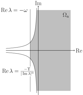
(a) Set $\Omega_{\rm a}$ considered in this paper.

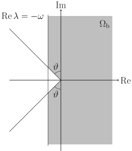
(b) Set $\Omega_{\rm b}$ considered in [38].

Figure 1. Comparison of sets that contain only finitely many eigenvalues.

Another important difference from [38] is an assumption on the control operator $B$ and the feedback operator $F$. Let $b,f\in X$ and let $B,F$ be written as $Bu=bu$ for all $u\in\mathbb{C}$ and $Fx=\langle x,f\rangle$ for all $x\in X$. In this paper, we assume that

$$b \in\mathcal{D}^{\beta}\coloneqq\left\{x\in X:\sum_{n=1}^{\infty}|\lambda_{n}|^{2\beta}\,|\langle x,\psi_{n}\rangle|^{2}<\infty\right\}$$

$$f \in\mathcal{D}^{\gamma}_{*}\coloneqq\left\{x\in X:\sum_{n=1}^{\infty}|\lambda_{n}|^{2\gamma}\,|\langle x,\phi_{n}\rangle|^{2}<\infty\right\},$$

where $\beta,\gamma\geq 0$ satisfy one of the following conditions: (i) $\beta$ and $\gamma$ are integers and $\beta+\gamma\geq\alpha$; or (ii) $\beta+\gamma>\alpha$. On the other hand, it is assumed in [38] that

$$b\in D(A^{-1})=\left\{x\in X:\sum_{n=1}^{\infty}\frac{|\langle x,\psi_{n}\rangle|^{2}}{|\lambda_{n}|^{2}}<\infty\right\}$$

and $f\in X$. Under the assumption we make in this paper, $B$ and $F$ have the parameters $\beta$ and $\gamma$ for design flexibility, which increases the applicability of the proposed robustness analysis.

The bounded linear operator $\Delta(\tau)$ on $X$ defined by

$$\Delta(\tau)\coloneqq T(\tau)+\int^{\tau}_{0}T(s)BFds$$

plays a key role in the analysis of robustness with respect to sampling. In fact, the sampled-data system (1) is strongly stable if and only if the discrete semigroup $(\Delta(\tau)^{k})_{k\in\mathbb{N}}$ is strongly stable, i.e.,

$$\lim_{k\to\infty}\|\Delta(\tau)^{k}x^{0}\|=0$$

for all $x^{0}\in X$. In [38], the sufficient condition for strong stability obtained in the Arendt-Batty-Lyubich-Vũ theorem [1, 19] is used in order to show that $(\Delta(\tau)^{k})_{k\in\mathbb{N}}$ is strongly stable. This sufficient condition requires that the intersection of the spectrum of $\Delta(\tau)$ and the unit circle be countable, but the system we consider does not have this property in general. Instead of the Arendt-Batty-Lyubich-Vũ theorem, we here employ the characterization of strong stability by an integral condition on resolvents developed in [36].

Let $0<\delta\leq\alpha/2$, where $\alpha>0$ is the constant for the set $\Omega_{\rm a}$. We give an integral condition on resolvents under which the orbit $\Delta(\tau)^{k}x^{0}$ with $x^{0}\in\mathcal{D}^{\delta}$ satisfies

$$\|\Delta(\tau)^{k}x^{0}\|=\begin{cases}o(k^{-\delta/\alpha})&\text{if $0<\delta<\alpha/2$}\vspace{5pt}\\ o\left(\sqrt{\dfrac{\log k}{k}}\right)&\text{if $\delta=\alpha/2$}\end{cases}$$

as $k\to\infty$. Using this integral condition, we show that the state $x$ of the sampled-data system (1) with sufficiently small sampling period $\tau>0$ satisfies

(2) $$\|x(t)\|=\begin{cases}o(t^{-\delta/\alpha})&\text{if $0<\delta<\alpha/2$}\vspace{5pt}\\ o\left(\sqrt{\dfrac{\log t}{t}}\right)&\text{if $\delta=\alpha/2$}\end{cases}$$

as $t\to\infty$ for every initial state $x^{0}\in\mathcal{D}^{\delta}$, provided that $\delta\leq 1$ or $\beta\geq\alpha$. Considering the open-loop case $F=0$, we see that $t^{-\delta/\alpha}$ in the estimate (2) cannot be replaced by functions with better decay rates. It is still unknown whether the logarithmic factor $\sqrt{\log t}$ in the case $\delta=\alpha/2$ may be removed.

The paper is organized as follows. Section 2 contains preliminaries on polynomial stability of $C_{0}$-semigroups and Riesz-spectral operators. In Section 3, we present the main result and introduce the discretized system for its proof. Section 4 is devoted to resolvent conditions for stability. To apply these conditions to the discretized system, we investigate the spectrum of $\Delta(\tau)$ in Section 5. Section 6 completes the proof of the main result with the help of the resolvent conditions for stability. To illustrate the theoretical result, we study a wave equation in Section 7. The conclusion is given in Section 8.

Notation and terminology

We denote by $\mathbb{N}_{0}$ the set of non-negative integers. For $\omega\in\mathbb{R}$ and $r>0$, we write

$$\mathbb{C}_{\omega} \coloneqq\{\lambda\in\mathbb{C}:\mathop{\rm Re}\nolimits\lambda>\omega\}$$

$$\mathbb{D}_{r} \coloneqq\{\lambda\in\mathbb{C}:|\lambda|<r\}$$

$$\mathbb{E}_{r} \coloneqq\{\lambda\in\mathbb{C}:|\lambda|>r\}.$$

Note that we denote the open right half-plane by $\mathbb{C}_{0}$, while $\mathbb{C}^{+}$ and $\mathbb{C}_{+}$ are commonly used in the literature. For $\alpha,\Upsilon>0$, define

$$\Omega_{\alpha,\Upsilon}\coloneqq\left\{\lambda\in\mathbb{C}\setminus\mathbb{R}:\mathop{\rm Re}\nolimits\lambda\leq\frac{-\Upsilon}{|\mathop{\rm Im}\nolimits\lambda|^{\alpha}}\right\}.$$

The closure of a subset $\Omega$ of $\mathbb{C}$ and the complex conjugate of $\lambda\in\mathbb{C}$ are denoted by $\overline{\Omega}$ and $\overline{\lambda}$, respectively. For real-valued functions $f,g$ on $J\subset\mathbb{R}$, we write

$$f(t)=O\big{(}g(t)\big{)}\qquad(t\to\infty)$$

if there exist $M>0$ and $t_{0}\in J$ such that $f(t)\leq Mg(t)$ for all $t\geq t_{0}$, and similarly,

$$f(t)=o\big{(}g(t)\big{)}\qquad(t\to\infty)$$

if for any $\varepsilon>0$, there exists $t_{0}\in J$ such that $f(t)\leq\varepsilon g(t)$ for all $t\geq t_{0}$.

Let $X$ and $Y$ be Banach spaces. For a linear operator $A\colon X\to Y$, we denote by $D(A)$ and $\mathop{\rm ran}\nolimits(A)$ the domain and the range of $A$, respectively. The space of all bounded linear operators from $X$ to $Y$ is denoted by $\mathcal{L}(X,Y)$, and we write $\mathcal{L}(X)\coloneqq\mathcal{L}(X,X)$. For a linear operator $A\colon D(A)\subset X\to X$, we denote by $\sigma(A)$ and $\rho(A)$ the spectrum and the resolvent set of $A$, respectively. We write $R(\lambda,A)\coloneqq(\lambda I-A)^{-1}$ for $\lambda\in\rho(A)$. For a subset $S$ of $X$ and a linear operator $A\colon D(A)\subset X\to Y$, we denote by $A|_{S}$ the restriction of $A$ to $S$, i.e., $A|_{S}x=Ax$ with domain $D(A|_{S})\coloneqq D(A)\cap S$.

A $C_{0}$-semigroup $(T(t))_{t\geq 0}$ on a Banach space $X$ is called uniformly bounded if $\sup_{t\geq 0}\|T(t)\|<\infty$ and strongly stable if $\lim_{t\to\infty}T(t)x=0$ for all $x\in X$. By a discrete semigroup on $X$, we mean a family $(\Delta^{k})_{k\in\mathbb{N}}$ of operators, where $\Delta\in\mathcal{L}(X)$. A discrete semigroup $(\Delta^{k})_{k\in\mathbb{N}}$ on $X$ is called power bounded if $\sup_{k\in\mathbb{N}}\|\Delta^{k}\|<\infty$ and strongly stable if $\lim_{k\to\infty}\Delta^{k}x=0$ fo all $x\in X$.

An inner product on a Hilbert space is denoted by $\langle\cdot,\cdot\rangle$. For Hilbert spaces $Z$ and $W$, let $A^{*}$ denote the Hilbert space adjoint of a densely defined linear operator $A\colon D(A)\subset Z\to W$.

2. Preliminaries

In this section, we review the definition and some important properties of polynomially stable $C_{0}$-semigroups and Riesz-spectral operators.

2.1. Polynomially stable $C_{0}$-semigroups

We start by recalling the definition of polynomially stable $C_{0}$-semigroups. In Definition 3.2 of [3], polynomial stability of $C_{0}$-semigroups does not include uniform boundedness, but here we define polynomial stability to include uniform boundedness as in Definition 1.2 of semi-uniform stability in [4].

Definition 2.1.

A $C_{0}$-semigroup $(T(t))_{t\geq 0}$ on a Banach space $X$ generated by $A$ is polynomially stable with parameter $\alpha>0$ if the following three conditions are satisfied:

1. $(T(t))_{t\geq 0}$ is uniformly bounded;

2. $i\mathbb{R}\subset\rho(A)$; and

3. $\|T(t)A^{-1}\|=O(t^{-1/\alpha})$ as $t\to\infty$.

Let $A$ be the generator of a uniformly bounded $C_{0}$-semigroup $(T(t))_{t\geq 0}$ on a Hilbert space. Then $-A$ and $-A^{*}$ are sectorial in the sense of Chapter 2 of [15]. In particular, if $(T(t))_{t\geq 0}$ is a polynomially stable $C_{0}$-semigroup on a Hilbert space, then $A$ and $A^{*}$ are invertible, and hence the fractional powers $(-A)^{\alpha}$ and $(-A^{*})^{\alpha}$ are well defined for all $\alpha\in\mathbb{R}$. We refer, e.g., to Chapter 3 of [15] and Section II.5.3 of [11] for the details of fractional powers.

We use the following characterizations for polynomial decay of a $C_{0}$-semigroup on a Hilbert space. The proof can be found in Lemma 2.3 and Theorem 2.4 of [6]. See also Lemma 2.3 of [39] for the result on the decay rate of an individual orbit.

Theorem 2.2.

Let $(T(t))_{t\geq 0}$ be a uniformly bounded $C_{0}$-semigroup on a Hilbert space $X$ with generator $A$ such that $i\mathbb{R}\subset\rho(A)$. For fixed $\alpha,\delta>0$, the following statements are equivalent:

1. $\|T(t)A^{-1}\|=O(t^{-1/\alpha})$ as $t\to\infty$.

2. $\|T(t)(-A)^{-\delta}\|=O(t^{-\delta/\alpha})$ as $t\to\infty$.

3. $\|T(t)(-A)^{-\delta}x\|=o(t^{-\delta/\alpha})$ as $t\to\infty$ for all $x\in X$.

4. $\|R(is,A)\|=O(|s|^{\alpha})$ as $|s|\to\infty$.

5. $\displaystyle\sup_{\lambda\in\overline{\mathbb{C}_{0}}}\|R(\lambda,A)(-A)^{\alpha}\|<\infty$.

The following estimate given in Lemma 4 of [25] is useful in the robustness analysis of polynomial stability.

Lemma 2.3.

Let $A$ be the generator of a polynomially stable $C_{0}$-semigroup with parameter $\alpha>0$ on a Hilbert space $X$. Let $\beta,\gamma\geq 0$ satisfy $\beta+\gamma\geq\alpha$ and let $U$ be a Banach space. There exists a constant $M\geq 1$ such that if $B\in\mathcal{L}(U,X)$ and $F\in\mathcal{L}(X,U)$ satisfy $\mathop{\rm ran}\nolimits(B)\subset D((-A)^{\beta})$ and $\mathop{\rm ran}\nolimits(F^{*})\subset D((-A^{*})^{\gamma})$, then

$$\|FR(\lambda,A)B\|\leq M\|(-A)^{\beta}B\|\,\|(-A^{*})^{\gamma}F^{*}\|$$

for all $\lambda\in\overline{\mathbb{C}_{0}}$.

2.2. Riesz-spectral operators

Next we recall the definition of Riesz-spectral operators and briefly state their most relevant properties. We refer the reader to Section 3.2 of [9], Section 2.4 of [37], and Chapter 2 of [14] for more details.

Definition 2.4 (Definition 3.2.6 of [9]).

Let $X$ be a Hilbert space and let $A\colon D(A)\subset X\to X$ be a closed linear operator with simple eigenvalues $(\lambda_{n})_{n\in\mathbb{N}}$ and corresponding eigenvectors $(\phi_{n})_{n\in\mathbb{N}}$. We say that $A$ is a Riesz-spectral operator if the following two conditions are satisfied:

1. $(\phi_{n})_{n\in\mathbb{N}}$ is a Riesz basis; and

2. The set of eigenvalues $\{\lambda_{n}:n\in\mathbb{N}\}$ has at most finitely many accumulation points.

Let $A$ be a Riesz-spectral operator on a Hilbert space $X$ with simple eigenvalues $(\lambda_{n})_{n\in\mathbb{N}}$ and corresponding eigenvectors $(\phi_{n})_{n\in\mathbb{N}}$. Let $(\psi_{n})_{n\in\mathbb{N}}$ be the eigenvectors of the adjoint $A^{*}$ corresponding to the eigenvalues $(\overline{\lambda_{n}})_{n\in\mathbb{N}}$. Then $(\psi_{n})_{n\in\mathbb{N}}$ can be suitable scaled so that $(\phi_{n})_{n\in\mathbb{N}}$ and $(\psi_{n})_{n\in\mathbb{N}}$ are biorthogonal, i.e.,

$$\langle\phi_{n},\psi_{m}\rangle=\begin{cases}1&\text{if $n=m$}\\ 0&\text{otherwise}.\end{cases}$$

A sequence biorthogonal to a Riesz basis in $X$ is unique and also forms a Riesz basis in $X$. Throughout this paper, we set the sequence $(\psi_{n})_{n\in\mathbb{N}}$ of the eigenvectors of the adjoint $A^{*}$ so that $(\psi_{n})_{n\in\mathbb{N}}$ are biorthogonal to $(\phi_{n})_{n\in\mathbb{N}}$. Every $x\in X$ can be represented uniquely by

$$x=\sum_{n=1}^{\infty}\langle x,\psi_{n}\rangle\phi_{n}=\sum_{n=1}^{\infty}\langle x,\phi_{n}\rangle\psi_{n}.$$

Moreover, there exist constants $M_{\rm a},M_{\rm b}>0$ such that for all $x\in X$,

$$M_{\rm a}\sum_{n=1}^{\infty}|\langle x,\psi_{n}\rangle|^{2}\leq\| x\|^{2}\leq M_{\rm b}\sum_{n=1}^{\infty}|\langle x,\psi_{n}\rangle|^{2}$$

$$\frac{1}{M_{\rm b}}\sum_{n=1}^{\infty}|\langle x,\phi_{n}\rangle|^{2}\leq\| x\|^{2}\leq\frac{1}{M_{\rm a}}\sum_{n=1}^{\infty}|\langle x,\phi_{n}\rangle|^{2}.$$

We shall frequently use these inequalities without comment.

The Riesz-spectral operator $A$ has the following representation:

(3) $$Ax=\sum_{n=1}^{\infty}\lambda_{n}\langle x,\psi_{n}\rangle\phi_{n},\quad x\in D(A)$$

with domain

$$D(A)=\left\{x\in X:\sum_{n=1}^{\infty}|\lambda_{n}|^{2}\,|\langle x,\psi_{n}\rangle|^{2}<\infty\right\}.$$

The spectrum of the Riesz-spectral operator $A$ is the closure of its point spectrum, that is, $\sigma(A)=\overline{\{\lambda_{n}:n\in\mathbb{N}\}}$. For $\lambda\in\rho(A)$, the resolvent $R(\lambda,A)$ is given by

(4) $$R(\lambda,A)x=\sum_{n=1}^{\infty}\frac{1}{\lambda-\lambda_{n}}\langle x,\psi_{n}\rangle\phi_{n},\quad x\in X.$$

The Riesz-spectral operator $A$ generates a $C_{0}$-semigroup on $X$ if and only if $\sup_{n\in\mathbb{N}}\mathop{\rm Re}\nolimits\lambda_{n}<\infty$, and the $C_{0}$-semigroup $(T(t))_{t\geq 0}$ generated by $A$ can be written as

$$T(t)x=\sum_{n=1}^{\infty}e^{t\lambda_{n}}\langle x,\psi_{n}\rangle\phi_{n}$$

for all $x\in X$ and $t\geq 0$.

The adjoint $A^{*}$ is also a Riesz-spectral operator and is represented as

$$A^{*}x=\sum_{n=1}^{\infty}\overline{\lambda_{n}}\langle x,\phi_{n}\rangle\psi_{n},\quad x\in D(A^{*})$$

with domain

$$D(A^{*})=\left\{x\in X:\sum_{n=1}^{\infty}\left|\lambda_{n}\right|^{2}\,\left|\langle x,\phi_{n}\rangle\right|^{2}<\infty\right\}.$$

Moreover, the $C_{0}$-semigroup generated by $A^{*}$ is given by $(T(t)^{*})_{t\geq 0}$.

To make assumptions on the ranges of the control operator $B\in\mathcal{L}(\mathbb{C},X)$ and the adjoint of the feedback operator $F\in\mathcal{L}(X,\mathbb{C})$, we use the following subsets with parameters $\beta,\gamma\geq 0$:

$$\mathcal{D}^{\beta} \coloneqq\left\{x\in X:\sum_{n=1}^{\infty}|\lambda_{n}|^{2\beta}\,|\langle x,\psi_{n}\rangle|^{2}<\infty\right\}$$

$$\mathcal{D}_{*}^{\gamma} \coloneqq\left\{x\in X:\sum_{n=1}^{\infty}|\lambda_{n}|^{2\gamma}\,|\langle x,\phi_{n}\rangle|^{2}<\infty\right\}.$$

3. Stability of sampled-data systems

In this section, we present the system under consideration and state the main result. We also introduce the discretized system as the first step of its proof.

3.1. Main result

Let $X$ be a Hilbert space, and consider the following sampled-data system with state space $X$ and input space $\mathbb{C}$:

(5a) $$\dot{x}(t) =Ax(t)+Bu(t),\quad t\geq 0;\qquad x(0)=x^{0}\in X$$

(5b) $$u(t) =Fx(k\tau),\quad k\tau\leq t<(k+1)\tau,~{}k\in\mathbb{N}_{0},$$

where $x(t)\in X$ is the state, $u(t)\in\mathbb{C}$ is the control input, $\tau>0$ is the sampling period, $A\colon D(A)\subset X\to X$ is the generator of a $C_{0}$-semigroup $(T(t))_{t\geq 0}$ on $X$, $B\in\mathcal{L}(\mathbb{C},X)$ is the control operator, and $F\in\mathcal{L}(X,\mathbb{C})$ is the feedback operator.

Definition 3.1.

The sampled-data system (5) is called strongly stable if

$$\lim_{t\to\infty}\|x(t)\|=0$$

for every initial state $x^{0}\in X$.

To state the main result, we make the following assumption on the sampled-data system (5).

Assumption 3.2.

Let $A$ be a Riesz-spectral operator on a Hilbert space $X$ with simple eigenvalues $(\lambda_{n})_{n\in\mathbb{N}}$ and corresponding eigenvectors $(\phi_{n})_{n\in\mathbb{N}}$. Let $(\psi_{n})_{n\in\mathbb{N}}$ be the eigenvectors of $A^{*}$ such that $(\phi_{n})_{n\in\mathbb{N}}$ and $(\psi_{n})_{n\in\mathbb{N}}$ are biorthogonal. Let the control operator $B\in\mathcal{L}(\mathbb{C},X)$ and the feedback operator $F\in\mathcal{L}(X,\mathbb{C})$ be represented as

(6) $$Bu=bu,\quad u\in\mathbb{C};\qquad Fx=\langle x,f\rangle,\quad x\in X$$

for some $b,f\in X$. Assume that the operators $A$, $B$, and $F$ satisfy the following conditions:

1. There exist constants $\omega,\alpha,\Upsilon>0$ such that $\mathbb{C}_{-\omega}\cap(\mathbb{C}\setminus\Omega_{\alpha,\Upsilon})$ has only finite elements of $(\lambda_{n})_{n\in\mathbb{N}}$.

2. $\{\lambda_{n}:n\in\mathbb{N}\}\cap i\mathbb{R}=\emptyset$.

3. $A+BF$ generates a polynomially stable $C_{0}$-semigroup $(T_{BF}(t))_{t\geq 0}$ with parameter $\alpha$ on $X$.

4. There exist constants $\beta,\gamma\geq 0$ such that $b\in\mathcal{D}^{\beta}$, $f\in\mathcal{D}_{*}^{\gamma}$, and one of the following conditions holds:

   1. $\beta,\gamma\in\mathbb{N}_{0}$ and $\beta+\gamma\geq\alpha$.

   2. $\beta+\gamma>\alpha$.

By (A1), the Riesz-spectral operator $A$ generates a $C_{0}$-semigroup $(T(t))_{t\geq 0}$. Since $\sigma(A)=\overline{\{\lambda_{n}:n\in\mathbb{N}\}}$, it follows that $\sigma(A)\cap i\mathbb{R}=\emptyset$ under (A1) and (A2). The eigenvalues $(\lambda_{n})_{n\in\mathbb{N}}$ may approach $i\mathbb{R}$ asymptotically, and an upper bound of the asymptotic rate is represented by the parameter $\alpha$ given in (A1). Note that when $\lim_{\ell\to\infty}\mathop{\rm Re}\nolimits\lambda_{n_{\ell}}=0$ for some subsequence $(\lambda_{n_{\ell}})_{\ell\in\mathbb{N}}$, there does not exist a feedback operator $F\in\mathcal{L}(X,\mathbb{C})$ such that the $C_{0}$-semigroup $(T_{BF}(t))_{t\geq 0}$ generated by $A+BF$ is exponentially stable; see, e.g., Theorem 8.2.3 of [9]. We assume by (A4) that $B$ and $F$ have stronger boundedness properties related to the parameter $\alpha$ than the standard boundedness properties $B\in\mathcal{L}(\mathbb{C},X)$ and $F\in\mathcal{L}(X,\mathbb{C})$. Assumptions similar to (A4) are placed to perturbation operators in the robustness analysis of polynomial stability developed in [22, 23, 24]. Note that not all of (A1)–(A4) are imposed in every result. In fact, (A2) is not used in Section 5 except for Lemma 5.2, while (A3) is not imposed in Sections 6.1 and 6.2.

The following theorem is the main result of this paper, which shows that polynomial stability is robust with respect to sampling.

Theorem 3.3.

If Assumption 3.2 is satisfied, then there exists $\tau^{*}>0$ such that the following statements hold for all $\tau\in(0,\tau^{*})$:

1. The sampled-data system (5) is strongly stable.

2. Let $0<\delta\leq\alpha/2$, and assume that $\delta\leq 1$ or $\beta\geq\alpha$. Then, for every initial state $x^{0}\in\mathcal{D}^{\delta}$, the state $x$ of the sampled-data system (5) satisfies

   (7) $$\|x(t)\|=\begin{cases}o(t^{-\delta/\alpha})&\text{if $0<\delta<\alpha/2$}\vspace{5pt}\\ o\left(\sqrt{\dfrac{\log t}{t}}\right)&\text{if $\delta=\alpha/2$}\end{cases}$$

   as $t\to\infty$.

Let $\alpha,\delta>0$ and consider the case $F=0$ and $\lambda_{n}=-1/n^{\alpha}+in$ for $n\in\mathbb{N}$. Then Assumption 3.2 holds for all $B\in\mathcal{L}(\mathbb{C},X)$, where the constants $\beta$ and $\gamma$ in (A4) are chosen such that $\beta=0$ and $\gamma>\alpha$. We also have $\|T(t)(-A)^{-\delta}\|=O(t^{-\delta/\alpha})$ as $t\to\infty$, and this decay rate is optimal in the sense that $\liminf_{t\to\infty}t^{\delta/\alpha}\|T(t)(-A)^{-\delta}\|>0$. Therefore, one cannot replace $t^{-\delta/\alpha}$ in the estimate (7) by functions with better decay rates. Whether the logarithmic correction term $\sqrt{\log t}$ for the case $\delta=\alpha/2$ may be omitted remains open.

The assumption $\delta\leq 1$ implies $D(A)\subset\mathcal{D}^{\delta}$. On the other hand, the assumption $\beta\geq\alpha$ leads to the uniform boundedness of $\|R(z,T(\tau))S(\tau)\|$ on an annulus $\{z\in\mathbb{C}:1<|z|<1+\varepsilon\}$ with some sufficiently small $\varepsilon>0$ for a fixed $\tau>0$, where $S(\tau)\in\mathcal{L}(\mathbb{C},X)$ is defined by

(8) $$S(\tau)u\coloneqq\int^{\tau}_{0}T(s)Buds,\quad u\in\mathbb{C}.$$

We will employ these assumptions in Section 6.2.

The proof of Theorem 3.3 is divided into several steps. In the next subsection, we prove the equivalence between the stability of the sampled-data system (5) and that of the discretized system. Section 4 is devoted to resolvent conditions for the stability of discrete semigroups on Hilbert spaces. To apply these resolvent conditions, in Section 5, we investigate the spectrum of the operator that represents the dynamics of the discretized system. In Section 6, we complete the proof of Theorem 3.3, by using the resolvent conditions presented in Section 4.

3.2. Discretized system

For $t\geq 0$, define $\Delta(t)\in\mathcal{L}(X)$ by

$$\Delta(t)\coloneqq T(t)+S(t)F.$$

Then the state $x$ of the sampled-data system (5) satisfies

(9) $$x\big{(}(k+1)\tau\big{)}=\Delta(\tau)x(k\tau)$$

for all $k\in\mathbb{N}_{0}$, which we call the discretized system.

To prove Theorem 3.3, it suffices by the next result to investigate the discrete semigroup $(\Delta(\tau)^{k})_{k\in\mathbb{N}}$.

Proposition 3.4.

Let $A$ be the generator of a $C_{0}$-semigroup $(T(t))_{t\geq 0}$ on a Banach space $X$. Let $B\in\mathcal{L}(\mathbb{C},X)$ and $F\in\mathcal{L}(X,\mathbb{C})$. The following statements hold for a fixed $\tau>0$:

1. The sampled-data system (5) is strongly stable if and only if the discrete semigroup $(\Delta(\tau)^{k})_{k\in\mathbb{N}}$ is strongly stable.

2. Let $g\colon(0,\infty)\to\mathbb{R}$, and suppose that there exist constants $k_{0}\in\mathbb{N}$ and $M_{1},M_{2}>0$ such that for all $k\in\mathbb{N}$ with $k\geq k_{0}$ and all $s\in[0,\tau)$,

   (10) $$M_{1}g(k\tau)\leq g(k)\leq M_{2}g(k\tau+s).$$

   Then the state $x$ of the sampled-data system (5) with initial state $x^{0}\in X$ satisfies

   (11) $$\|x(t)\|=o\big{(}g(t)\big{)}\qquad(t\to\infty)$$

   if and only if $x^{0}$ satisfies

   (12) $$\|\Delta(\tau)^{k}x^{0}\|=o\big{(}g(k)\big{)}\qquad(k\to\infty).$$

Proof.

The statement a) has been proved in Proposition 2.2 in [38], and therefore we show only the statement b). Assume that (11) holds for the state $x$ of the sampled-data system (5) with initial state $x^{0}\in X$. Take $\varepsilon>0$. There exists $t_{1}>0$ such that for all $t\geq t_{1}$,

$$\|x(t)\|\leq\frac{\varepsilon}{M_{1}}g(t).$$

Choose $k_{1}\in\mathbb{N}$ so that $k_{1}\geq k_{0}$ and $k_{1}\tau\geq t_{1}$. By (9) and (10), we have that

$$\|\Delta(\tau)^{k}x^{0}\|=\|x(k\tau)\|\leq\frac{\varepsilon}{M_{1}}g(k\tau)\leq\varepsilon g(k)$$

for all $k\geq k_{1}$. Hence, (12) holds.

Conversely, assume that $x^{0}\in X$ satisfies (12), and take $\varepsilon>0$. We have that

$$1\leq K\coloneqq\sup_{0\leq s<\tau}\|\Delta(s)\|<\infty.$$

Then $\|x(k\tau+s)\|\leq K\|x(k\tau)\|$ for all $k\in\mathbb{N}_{0}$ and $s\in[0,\tau)$. By assumption, there exists $k_{2}\in\mathbb{N}$ such that for all $k\geq k_{2}$,

$$\|\Delta(\tau)^{k}x^{0}\|\leq\frac{\varepsilon}{KM_{2}}g(k).$$

Combining this estimate and (9), we obtain

$$\|x(k\tau+s)\|\leq\frac{\varepsilon}{M_{2}}g(k)$$

for all $k\geq k_{2}$ and $s\in[0,\tau)$. It follows from (10) that

$$\|x(k\tau+s)\|\leq\varepsilon g(k\tau+s)$$

for all $k\geq\max\{k_{0},k_{2}\}$ and $s\in[0,\tau)$. Thus, we obtain (11). ∎

We immediately see that the condition (10) holds for $g(t)\coloneqq t^{-\delta}$ with $\delta>0$. The function $g$ defined by

$$g(t)\coloneqq\sqrt{\frac{\log t}{t}}$$

also satisfies the condition (10). In fact, we obtain

$$\frac{\log(k\tau)}{k\tau} =\frac{\log(k\tau)}{\tau\log k}\cdot\frac{\log k}{k}$$

$$\frac{\log k}{k} =\frac{\frac{\log k}{\log(k\tau+s)}}{\frac{k}{k\tau+s}}\cdot\frac{\log(k\tau+s)}{k\tau+s}\leq\frac{\frac{\log k}{\log(k\tau)}}{\frac{k}{(k+1)\tau}}\cdot\frac{\log(k\tau+s)}{k\tau+s}$$

for all $k\in\mathbb{N}$ with $k>\max\{1,1/\tau\}$ and all $s\in[0,\tau)$. Therefore, there exists $k_{0}\in\mathbb{N}$ such that for all $k\geq k_{0}$ and $s\in[0,\tau)$,

$$\frac{\sqrt{\tau}}{2}\sqrt{\frac{\log(k\tau)}{k\tau}}\leq\sqrt{\frac{\log k}{k}}\leq 2\sqrt{\tau}\sqrt{\frac{\log(k\tau+s)}{k\tau+s}}.$$

4. Resolvent conditions for stability of discrete semigroups

First, we review resolvent characterizations of power boundedness and strong stability of discrete semigroups on Hilbert spaces. A resolvent characterization of power bounded discrete semigroups has been obtained in Theorem II.1.12 of [10], which is an analogue of the characterization of uniformly bounded $C_{0}$-semigroups due to [13, 35]. Moreover, a resolvent characterization of strongly stable discrete semigroups has been developed in Theorem 3.11 of [36]; see also Theorem II.2.23 of [10].

Theorem 4.1.

Let $X$ be a Hilbert space and let $\Delta\in\mathcal{L}(X)$ satisfy $\mathbb{E}_{1}\subset\rho(\Delta)$. Then the following statements hold:

1. The discrete semigroup $(\Delta^{k})_{k\in\mathbb{N}}$ is power bounded if and only if

   $$\limsup_{r\downarrow 1}\,(r-1)\int^{2\pi}_{0}\|R(re^{i\theta},\Delta)x\|^{2}d\theta <\infty\quad\text{for all $x\in X$ and}$$

   $$\limsup_{r\downarrow 1}\,(r-1)\int^{2\pi}_{0}\|R(re^{i\theta},\Delta)^{*}y\|^{2}d\theta <\infty\quad\text{for all $y\in X$.}$$

2. The discrete semigroup $(\Delta^{k})_{k\in\mathbb{N}}$ is strongly stable if and only if

   $$\lim_{r\downarrow 1}\,(r-1)\int^{2\pi}_{0}\|R(re^{i\theta},\Delta)x\|^{2}d\theta =0\quad\text{for all $x\in X$ and}$$

   $$\limsup_{r\downarrow 1}\,(r-1)\int^{2\pi}_{0}\|R(re^{i\theta},\Delta)^{*}y\|^{2}d\theta <\infty\quad\text{for all $y\in X$.}$$

Next, we investigate a resolvent condition on the rate of decay for discrete semigroups on Hilbert spaces. To this end, the following equalities given in Lemma II.1.11 of [10] are useful.

Lemma 4.2.

Let $X$ be a Banach space and let $\Delta\in\mathcal{L}(X)$ with spectral radius $\mathop{\rm r}\nolimits(\Delta)$. Then

$$\Delta^{k}=\frac{r^{k+1}}{2\pi}\int^{2\pi}_{0}e^{i\theta(k+1)}R(re^{i\theta},\Delta)d\theta=\frac{r^{k+2}}{2\pi(k+1)}\int^{2\pi}_{0}e^{i\theta(k+1)}R(re^{i\theta},\Delta)^{2}d\theta$$

for all $k\in\mathbb{N}$ and $r>\mathop{\rm r}\nolimits(\Delta)$.

We state the discrete analogue of Lemma 3.2 in [39].

Proposition 4.3.

Let $(\Delta^{k})_{k\in\mathbb{N}}$ be a power bounded discrete semigroup on a Hilbert space $X$. The following statements hold for a fixed $x\in X$:

1. If $\|\Delta^{k}x\|=o(k^{-\delta})$ as $k\to\infty$ for some $0<\delta\leq 1/2$, then

   (13) $$\lim_{r\downarrow 1}\Lambda_{\delta}(r)\int^{2\pi}_{0}\|R(re^{i\theta},\Delta)x\|^{2}d\theta=0,$$

   where

   $$\Lambda_{\delta}(r)\coloneqq\begin{cases}(r-1)^{1-2\delta}&\text{if $0<\delta<1/2$}\\ |\log(r-1)|^{-1}&\text{if $\delta=1/2$.}\end{cases}$$

2. If (13) holds for some $0<\delta<1/2$, then $\|\Delta^{k}x\|=o(k^{-\delta})$ as $k\to\infty$. On the other hand, if (13) holds for $\delta=1/2$, then

   $$\|\Delta^{k}x\|=o\left(\sqrt{\frac{\log k}{k}}\right)\qquad(k\to\infty).$$

Proof.

a) Assume that $x\in X$ satisfies $\|\Delta^{k}x\|=o(k^{-\delta})$ as $k\to\infty$ for some $0<\delta\leq 1/2$. Take $\varepsilon>0$ and $1<r<2$. There exists $k_{0}\in\mathbb{N}$ such that

(14) $$\|\Delta^{k}x\|^{2}\leq\frac{\varepsilon}{k^{2\delta}}$$

for all $k\geq k_{0}$. We obtain

(15) $$\frac{1}{2\pi}\int^{2\pi}_{0}\|R(re^{i\theta},\Delta)x\|^{2}d\theta=\sum_{k=-\infty}^{\infty}\left\|\frac{1}{2\pi}\int^{2\pi}_{0}e^{ik\theta}R(re^{i\theta},\Delta)xd\theta\right\|^{2}$$

by Parseval’s equality for vector-valued functions, which can be proved by the scalar-valued Parseval’s equality as done for Plancherel’s theorem in Section 1.8 of [2]. Noting that the first equality in Lemma 4.2 is true also for $k=0$, we have for each positive integer $k$,

$$\frac{1}{2\pi}\int^{2\pi}_{0}e^{ik\theta}R(re^{i\theta},\Delta)xd\theta=\frac{\Delta^{k-1}x}{r^{k}}.$$

On the other hand, Cauchy’s integral theorem implies that for each non-positive integer $k$,

$$\int^{2\pi}_{0}e^{ik\theta}R(re^{i\theta},\Delta)xd\theta=-ir^{-k}\int_{\mathbb{T}_{1/r}}z^{-k}(I-z\Delta)^{-1}xdz=0.$$

Therefore, we have from the equality (15) that

$$\frac{1}{2\pi}\int^{2\pi}_{0}\|R(re^{i\theta},\Delta)x\|^{2}d\theta=\sum_{k=0}^{\infty}\frac{\|\Delta^{k}x\|^{2}}{r^{2(k+1)}}.$$

Since $(\Delta^{k})_{k\in\mathbb{N}}$ is power bounded, it follows that $M\coloneqq\sup_{k\in\mathbb{N}_{0}}\|\Delta^{k}\|<\infty$. Hence

$$\sum_{k=0}^{k_{0}-1}\frac{\|\Delta^{k}x\|^{2}}{r^{2(k+1)}}\leq k_{0}M^{2}\|x\|^{2}.$$

First suppose that $0<\delta<1/2$. Then the estimate (14) yields

$$\sum_{k=k_{0}}^{\infty}\frac{\|\Delta^{k}x\|^{2}}{r^{2(k+1)}}\leq\frac{\varepsilon}{r^{2}}\sum_{k=k_{0}}^{\infty}\frac{1}{k^{2\delta}r^{2k}}\leq\frac{\varepsilon}{r^{2}}\int_{0}^{\infty}\frac{1}{t^{2\delta}r^{2t}}dt.$$

We have that

$$\int_{0}^{\infty}\frac{1}{t^{2\delta}r^{2t}}dt=\int_{0}^{\infty}\frac{e^{-2t\log r}}{t^{2\delta}}dt=\frac{\Gamma(1-2\delta)}{(2\log r)^{1-2\delta}},$$

where $\Gamma$ is the Gamma function. Since

$$\frac{\log(v+1)}{v}\geq\frac{1}{2}$$

for all $0<v<1$, it follows that

$$\sum_{k=k_{0}}^{\infty}\frac{\|\Delta^{k}x\|^{2}}{r^{2(k+1)}}\leq\frac{\varepsilon\Gamma(1-2\delta)}{r^{2}(r-1)^{1-2\delta}}.$$

Hence

$$\limsup_{r\downarrow 1}\,(r-1)^{1-2\delta}\sum_{k=0}^{\infty}\frac{\|\Delta^{k}x\|^{2}}{r^{2(k+1)}}\leq\limsup_{r\downarrow 1}\,(r-1)^{1-2\delta}k_{0}M^{2}\|x\|^{2}+\limsup_{r\downarrow 1}\,\frac{\varepsilon\Gamma(1-2\delta)}{r^{2}}\leq\varepsilon\Gamma(1-2\delta).$$

Since $\varepsilon>0$ was arbitrary, the desired conclusion (13) holds for $0<\delta<1/2$.

Next we consider the case $\delta=1/2$. By the well-known formula for the first polylogarithm (see, e.g., p. 3 of [16]), we obtain

$$\sum_{k=1}^{\infty}\frac{1}{kr^{2k}}=\log\frac{r^{2}}{r^{2}-1}.$$

Moreover,

$$\log\frac{r^{2}}{r^{2}-1}=\log\frac{r}{r-1}+\log\frac{r}{r+1}\leq\log\frac{r}{r-1}=\log r+|\log(r-1)|.$$

Therefore, the estimate (14) gives

$$\sum_{k=k_{0}}^{\infty}\frac{\|\Delta^{k}x\|^{2}}{r^{2(k+1)}}\leq\frac{\varepsilon}{r^{2}}\sum_{k=k_{0}}^{\infty}\frac{1}{kr^{2k}}\leq\frac{\varepsilon}{r^{2}}(\log r+|\log(r-1)|).$$

Since $|\log(r-1)|^{-1}\to 0$ as $r\downarrow 1$, we have

$$\limsup_{r\downarrow 1}\,|\log(r-1)|^{-1}\sum_{k=0}^{\infty}\frac{\|\Delta^{k}x\|^{2}}{r^{2(k+1)}}\leq\limsup_{r\downarrow 1}\,|\log(r-1)|^{-1}\left(k_{0}M^{2}\|x\|^{2}+\frac{\varepsilon\log r}{r^{2}}\right)+\limsup_{r\downarrow 1}\,\frac{\varepsilon}{r^{2}}\leq\varepsilon.$$

This proves that (13) holds for $\delta=1/2$.

b) By Lemma 4.2 and the Cauchy-Schwartz inequality, we have that for all $x,y\in X$, $r>1$, and $k\in\mathbb{N}$,

$$|\langle\Delta^{k}x,y\rangle| \leq\frac{r^{k+2}}{2\pi(k+1)}\int^{2\pi}_{0}|\langle R(re^{i\theta},\Delta)^{2}x,y\rangle|d\theta$$

$$=\frac{r^{k+2}}{2\pi(k+1)}\int^{2\pi}_{0}|\langle R(re^{i\theta},\Delta)x,R(re^{-i\theta},\Delta^{*})y\rangle|d\theta$$

$$\leq\frac{r^{k+2}}{2\pi(k+1)}\left(\int^{2\pi}_{0}\|R(re^{i\theta},\Delta)x\|^{2}d\theta\right)^{1/2}\left(\int^{2\pi}_{0}\|R(re^{i\theta},\Delta^{*})y\|^{2}d\theta\right)^{1/2}.$$

Take $r_{1}>1$. Since $(\Delta^{k})_{k\in\mathbb{N}}$ is power bounded, Theorem 4.1.a) and the uniform boundedness principle imply that there exists a constant $M_{1}>0$ such that

$$(r-1)\int^{2\pi}_{0}\|R(re^{i\theta},\Delta^{*})y\|^{2}d\theta\leq M_{1}^{2}\|y\|^{2}$$

for all $y\in X$ and $r\in(1,r_{1})$. Hence

$$\|\Delta^{k}x\|\leq\frac{M_{1}}{2\pi}\cdot\frac{r^{k+2}}{(k+1)(r-1)}\sqrt{\frac{r-1}{\Lambda_{\delta}(r)}}\left(\Lambda_{\delta}(r)\int^{2\pi}_{0}\|R(re^{i\theta},\Delta)x\|^{2}d\theta\right)^{1/2}$$

for all $x\in X$ and $r\in(1,r_{1})$. Put $r\coloneqq 1+\frac{1}{k+1}$. Then

$$\frac{r^{k+2}}{(k+1)(r-1)}=\left(1+\frac{1}{k+1}\right)^{k+2}\to e\qquad(k\to\infty).$$

Moreover, we obtain

$$\frac{r-1}{\Lambda_{\delta}(r)} =\begin{cases}(k+1)^{-2\delta}&\text{if $0<\delta<1/2$}\vspace{5pt}\\ \dfrac{\log(k+1)}{k+1}&\text{if $\delta=1/2$}.\end{cases}$$

Hence, there exists $k_{1}\in\mathbb{N}$ such that for all $k\geq k_{1}$,

$$\frac{r^{k+2}}{(k+1)(r-1)}\sqrt{\frac{r-1}{\Lambda_{\delta}(r)}}\leq\begin{cases}2ek^{-\delta}&\text{if $0<\delta<1/2$}\vspace{5pt}\\ 2e\sqrt{\dfrac{\log k}{k}}&\text{if $\delta=1/2$}.\end{cases}$$

Combining this estimate with (13), we obtain $\|\Delta^{k}x\|=o(k^{-\delta})$ as $k\to\infty$ for $0<\delta<1/2$ and

$$\|\Delta^{k}x\|=o\left(\sqrt{\frac{\log k}{k}}\right)$$

as $k\to\infty$ for $\delta=1/2$. ∎

5. Spectrum and sampling

To apply Theorem 4.1 to the discretized system (9), we have to show that $\mathbb{E}_{1}\subset\rho(\Delta(\tau))$ is satisfied. The aim of this section is to prove the following theorem.

Theorem 5.1.

If (A1), (A3), and (A4) hold, then there exists $\tau^{*}>0$ such that $\mathbb{E}_{1}\subset\rho(\Delta(\tau))$ for all $\tau\in(0,\tau^{*})$.

First, we apply a spectral decomposition for $A$. Next, we prove the inclusion $\mathcal{D}^{\beta}\subset D((-A-BF)^{\widetilde{\beta}})$ for all $\widetilde{\beta}\in[0,\beta)$. Using this inclusion, we also show that $|1-F(\lambda I-A)^{-1}B|$ is bounded from below by a positive constant on $\rho(A)\cap\overline{\mathbb{C}_{0}}$. This estimate for the continuous-time system leads to an analogous estimate for the discretized system, i.e., a lower bound of $|1-F(zI-T(\tau))^{-1}S(\tau)|$ on $\rho(T(\tau))\cap\overline{\mathbb{E}_{1}}$. Finally, the desired inclusion $\mathbb{E}_{1}\subset\rho(\Delta(\tau))$ is proved.

5.1. Spectral decomposition

We start by applying a spectral decomposition for $A$ under (A1). A more general version of spectral decompositions for unbounded operators can be found in Lemma 2.4.7 of [9] and Proposition IV.1.16 of [11].

Since only finite elements of $(\lambda_{n})_{n\in\mathbb{N}}$ are in $\mathbb{C}_{-\omega}\cap(\mathbb{C}\setminus\Omega_{\alpha,\Upsilon})$, there exists a smooth, positively oriented, and simple closed curve $\Phi$ in $\rho(A)$ containing $\sigma(A)\cap\mathbb{C}_{0}$ in its interior and $\sigma(A)\cap(\mathbb{C}\setminus\mathbb{C}_{0})$ in its exterior. The operator

(16) $$\Pi\coloneqq\frac{1}{2\pi i}\int_{\Phi}(\lambda I-A)^{-1}d\lambda$$

is a projection on $X$ and yields the decomposition

$$X=X^{+}\oplus X^{-},$$

where

$$X^{+}\coloneqq\Pi X,\quad X^{-}\coloneqq(I-\Pi)X.$$

We have that $\dim X^{+}<\infty$. Moreover, $X^{+}$ and $X^{-}$ are $T(t)$-invariant for all $t\geq 0$. Define

$$A^{+}\coloneqq A|_{X^{+}},\quad A^{-}\coloneqq A|_{X^{-}}.$$

Then

$$\sigma(A^{+})=\sigma(A)\cap\mathbb{C}_{0},\quad\sigma(A^{-})=\sigma(A)\cap(\mathbb{C}\setminus\mathbb{C}_{0}).$$

Let $N_{\rm a},N_{\rm b}\in\mathbb{N}$ satisfy

(17) $$\{\lambda_{n}:1\leq n\leq N_{\rm a}-1\} =\{\lambda_{n}:n\in\mathbb{N}\}\cap\mathbb{C}_{0}=\sigma(A^{+})$$

(18) $$\{\lambda_{n}:1\leq n\leq N_{\rm b}-1\} =\{\lambda_{n}:n\in\mathbb{N}\}\cap\big{(}\mathbb{C}_{-\omega}\cap(\mathbb{C}\setminus\Omega_{\alpha,\Upsilon})\big{)}$$

by changing the order of $(\lambda_{n})_{n\in\mathbb{N}}$ if necessary. By construction, we obtain $N_{\rm b}\geq N_{\rm a}$. The series expansions of $A^{+}$ and $A^{-}$ are given by

$$A^{+}x^{+} =\sum_{n=1}^{N_{\rm a}-1}\lambda_{n}\langle x^{+},\psi_{n}\rangle\phi_{n}\quad\text{for all~{}}x^{+}\in D(A^{+})=X^{+}$$

$$A^{-}x^{-} =\sum_{n=N_{\rm a}}^{\infty}\lambda_{n}\langle x^{-},\psi_{n}\rangle\phi_{n}\quad\text{for all~{}}x^{-}\in D(A^{-})=\left\{x^{-}\in X^{-}:\sum_{n=N_{\rm a}}^{\infty}|\lambda_{n}|^{2}\,|\langle x^{-},\psi_{n}\rangle|^{2}<\infty\right\}.$$

For all $\lambda\in\rho(A)$, $X^{+}$ and $X^{-}$ are $(\lambda I-A)^{-1}$-invariant and

$$(\lambda I-A^{+})^{-1}=(\lambda I-A)^{-1}|_{X^{+}},\quad(\lambda I-A^{-})^{-1}=(\lambda I-A)^{-1}|_{X^{-}}.$$

For $t\geq 0$, we define

$$T^{+}(t)\coloneqq T(t)|_{X^{+}},\quad T^{-}(t)\coloneqq T(t)|_{X^{-}}.$$

Then $(T^{+}(t))_{t\geq 0}$ and $(T^{-}(t))_{t\geq 0}$ are $C_{0}$-semigroups with generators $A^{+}$ and $A^{-}$, respectively. The adjoint $\Pi^{*}$ is also a projection on $X$ and yields a spectral decomposition for $A^{*}$. We define

$$X^{+}_{*}\coloneqq\Pi^{*}X,\quad X^{-}_{*}\coloneqq(I-\Pi^{*})X.$$

The restriction $A^{-}_{*}\coloneqq A^{*}|_{X^{-}_{*}}$ of the adjoint $A^{*}$ is the generator of a $C_{0}$-semigroup $(T^{-}_{*}(t))_{t\geq 0}$, where

$$T^{-}_{*}(t)\coloneqq T(t)^{*}|_{X^{-}_{*}}$$

for $t\geq 0$. Define

$$B^{+}\coloneqq\Pi B,\quad B^{-}\coloneqq(I-\Pi)B,\quad F^{+}\coloneqq F|_{X^{+}},\quad F^{-}\coloneqq F|_{X^{-}}.$$

From (6), we have that

$$B^{+}u=b^{+}u,\quad B^{-}u=b^{-}u\quad \text{for all~{}}u\in\mathbb{C}$$

$$F^{+}x^{+}=\langle x^{+},f^{+}\rangle\quad \text{for all~{}}x^{+}\in X^{+}$$

$$F^{-}x^{-}=\langle x^{-},f^{-}\rangle\quad \text{for all~{}}x^{-}\in X^{-},$$

where $b^{+}\coloneqq\Pi b$, $b^{-}\coloneqq(I-\Pi)b$, $f^{+}\coloneqq\Pi^{*}f$, and $f^{-}\coloneqq(I-\Pi^{*})f$.

The polynomial stability of $(T^{-}(t))_{t\geq 0}$ and $(T^{-}_{*}(t))_{t\geq 0}$ under (A1) and (A2) is an immediate consequence of the equivalence between a) and c) in Theorem 2.2.

Lemma 5.2.

If (A1) and (A2) hold, then the $C_{0}$-semigroups $(T^{-}(t))_{t\geq 0}$ and $(T^{-}_{*}(t))_{t\geq 0}$ constructed as above are polynomially stable with parameter $\alpha$.

5.2. Inclusion $\mathcal{D}^{\beta}\subset D((-A-BF)^{\widetilde{\beta}})$ for $0\leq\widetilde{\beta}<\beta$

Let a Riesz-spectral operator $A$ on a Hilbert space $X$ generate a $C_{0}$-semigroup. Let $B\in\mathcal{L}(\mathbb{C},X)$ and $F\in\mathcal{L}(X,\mathbb{C})$ be such that $A+BF$ is the generator of a uniformly bounded $C_{0}$-semigroup. Then, the fractional power $(-A-BF)^{\beta}$ is well defined for every $\beta>0$. We will show that if $\mathop{\rm ran}\nolimits(B)\subset\mathcal{D}^{\beta}$ for some $\beta>0$, then $\mathcal{D}^{\beta}\subset D((-A-BF)^{\widetilde{\beta}})$ holds for all $\widetilde{\beta}\in[0,\beta)$. To this end, the following result is useful; see Lemma 5.4 of [39] for the proof.

Lemma 5.3.

Let $X$ be a Banach space and let $V\in\mathcal{L}(X)$. Suppose that $A$ and $A+V$ are the generators of exponentially stable $C_{0}$-semigroups on $X$. Then $D((-A)^{\alpha_{1}})\subset D((-A-V)^{\alpha_{2}})$ for all $\alpha_{1},\alpha_{2}\in(0,1)$ with $\alpha_{2}<\alpha_{1}$.

We investigate the relation between $D(A^{n})$ and $D((A+BF)^{n})$ for $n\in\mathbb{N}$.

Lemma 5.4.

Let $A$ be a linear operator on a Banach space $X$ and let $F\in\mathcal{L}(X,\mathbb{C})$. Define $B\in\mathcal{L}(\mathbb{C},X)$ by $Bu\coloneqq bu$ for $u\in\mathbb{C}$, where $b\in X$. Then the following assertion holds for all $n\in\mathbb{N}$: If $x\in D(A^{n})$ and $b\in D(A^{n-1})$, then $x\in D((A+BF)^{n})$ and

(19) $$(A+BF)^{n}x=A^{n}x+q_{n-1}A^{n-1}b+\cdots+q_{0}b,$$

where $q_{m}\coloneqq F(A+BF)^{n-m-1}x\in\mathbb{C}$ for $m=0,\dots,n-1$.

Proof.

We prove the assertion by induction. In the case $n=1$, $x\in D(A)$ satisfies $x\in D(A+BF)$ and $(A+BF)x=Ax+(Fx)b$. Now, assume that the assertion holds for some $n\in\mathbb{N}$. Let $x\in D(A^{n+1})$ and $b\in D(A^{n})$. Then $A^{n}x\in D(A)$ and

$$A^{m}b\in D(A)$$

for all $m=0,\dots,n-1$. This and the inductive assumption imply

$$(A+BF)^{n}x\in D(A)=D(A+BF),$$

and hence $x\in D((A+BF)^{n+1})$. Moreover,

$$(A+BF)^{n+1}x =A(A^{n}x+(Fx)A^{n-1}b+\cdots+(F(A+BF)^{n-1}x)b)+BF(A+BF)^{n}x$$

$$=A^{n+1}x+(Fx)A^{n}b+\cdots+(F(A+BF)^{n-1}x)Ab+(F(A+BF)^{n}x)b.$$

Thus, (19) holds when $n$ is replaced by $n+1$. ∎

Combining Lemmas 5.3 and 5.4, we obtain the following result.

Lemma 5.5.

Let $A$ be a Riesz-spectral operator on a Hilbert space $X$ with simple eigenvalues $(\lambda_{n})_{n\in\mathbb{N}}$ such that $\sup_{n\in\mathbb{N}}\mathop{\rm Re}\nolimits\lambda_{n}<\infty$ and $0$ is not an accumulation point of the set $\{\lambda_{n}:n\in\mathbb{N}\}$. Define $B\in\mathcal{L}(\mathbb{C},X)$ by $Bu\coloneqq bu$ for $u\in\mathbb{C}$, where $b\in\mathcal{D}^{\beta}$ for some $\beta>0$. Let $F\in\mathcal{L}(X,\mathbb{C})$ be such that $A+BF$ generates a uniformly bounded $C_{0}$-semigroup on $X$. Then for all $\widetilde{\beta}\in[0,\beta)$, one has $\mathcal{D}^{\beta}\subset D((-A-BF)^{\widetilde{\beta}})$; in particular $b\in D((-A-BF)^{\widetilde{\beta}})$.

Proof.

There exists $h>0$ such that $A_{h}\coloneqq A-hI$ generates an exponentially stable $C_{0}$-semigroup on $X$. To prove that $\mathcal{D}^{\beta}=D((-A_{h})^{\beta})$, we take $r>0$ so that $\mathbb{D}_{r}$ has a finite number of the eigenvalues $(\lambda_{n})_{n\in\mathbb{N}}$. Let $N_{r}\in\mathbb{N}$ satisfy

$$\{\lambda_{n}:1\leq n\leq N_{r}-1\}=\{\lambda_{n}:n\in\mathbb{N}\}\cap\mathbb{D}_{r}$$

by changing the order of $(\lambda_{n})_{n\in\mathbb{N}}$ if necessary. We decompose $x\in X$ into

$$x=\sum_{n=1}^{N_{r}-1}\langle x,\psi_{n}\rangle\phi_{n}+\sum_{n=N_{r}}^{\infty}\langle x,\psi_{n}\rangle\phi_{n}\eqqcolon x_{1}+x_{2}.$$

By construction, $x_{1}\in\mathcal{D}^{\beta}\cap D((-A_{h})^{\beta})$. Since $\inf_{n\geq N_{r}}|\lambda_{n}|\geq r>0$, the equivalence between $x_{2}\in\mathcal{D}^{\beta}$ and $x_{2}\in D((-A_{h})^{\beta})$ follows as in the proof of Lemma 3.2.11.c of [9]. Therefore, we obtain $\mathcal{D}^{\beta}=D((-A_{h})^{\beta})$.

Since

$$D\big{(}(-A_{h})^{\beta}\big{)}\subset D\Big{(}(-A_{h})^{\widetilde{\beta}}\Big{)},\quad D\big{(}(-A-BF)^{\beta}\big{)}\subset D\Big{(}(-A-BF)^{\widetilde{\beta}}\Big{)}$$

for every $\widetilde{\beta}\in[0,\beta)$, it suffices to consider the case where $n<\widetilde{\beta}<\beta<n+1$ for some $n\in\mathbb{N}_{0}$. Put $\beta_{0}\coloneqq\beta-n$ and $\widetilde{\beta}_{0}\coloneqq\widetilde{\beta}-n$. Take $x\in\mathcal{D}^{\beta}=D((-A_{h})^{\beta})$. We have from the first law of exponents (see, e.g., Proposition 3.1.1.c) of [15]) that

(20) $$D\big{(}(-A_{h})^{\beta}\big{)} =\left\{x\in D(A_{h}^{n}):A_{h}^{n}x\in D\big{(}(-A_{h})^{\beta_{0}}\big{)}\right\}$$

(21) $$D\Big{(}(-A_{h}-BF)^{\widetilde{\beta}}\Big{)} =\left\{x\in D\big{(}(A_{h}+BF)^{n}\big{)}:(A_{h}+BF)^{n}x\in D\Big{(}(-A_{h}-BF)^{\widetilde{\beta}_{0}}\Big{)}\right\}.$$

Since $x,b\in D(A_{h}^{n})$, Lemma 5.4 implies that $x\in D((A_{h}+BF)^{n})$ and

(22) $$(A_{h}+BF)^{n}x=A_{h}^{n}x+q_{n-1}A_{h}^{n-1}b+\cdots+q_{0}b$$

for some $q_{0},\dots,q_{n-1}\in\mathbb{C}$. By $b\in D(A_{h}^{n})$,

$$A_{h}^{m}b\in D(A_{h})\subset D\big{(}(-A_{h})^{\beta_{0}}\big{)}$$

for all $m=0,\dots,n-1$. Moreover, we have from $x\in D((-A_{h})^{\beta})$ and (20) that

$$A_{h}^{n}x\in D\big{(}(-A_{h})^{\beta_{0}}\big{)}.$$

Hence $(A_{h}+BF)^{n}x\in D((-A_{h})^{\beta_{0}})$ by (22). Lemma 5.3 yields

$$D\big{(}(-A_{h})^{\beta_{0}}\big{)}\subset D\Big{(}(-A_{h}-BF)^{\widetilde{\beta}_{0}}\Big{)},$$

and therefore

$$(A_{h}+BF)^{n}x\in D\Big{(}(-A_{h}-BF)^{\widetilde{\beta}_{0}}\Big{)}.$$

This and (21) give $x\in D((-A_{h}-BF)^{\widetilde{\beta}})$. Since $D((-A_{h}-BF)^{\widetilde{\beta}})=D((-A-BF)^{\widetilde{\beta}})$ by Proposition 3.1.9.a) of [15], we conclude that $\mathcal{D}^{\beta}\subset D((-A-BF)^{\widetilde{\beta}})$. ∎

5.3. Lower bound of $|1-FR(z,T(\tau))S(\tau)|$

In this subsection, we complete the proof of Theorem 5.1, by showing that $|1-FR(z,T(\tau))S(\tau)|$ is bounded from below by a positive constant on $\rho(T(\tau))\cap\overline{\mathbb{E}_{1}}$. First, we estimate $|FR(\lambda,A+BF)B|$ with the help of Lemma 5.5.

Lemma 5.6.

If (A1), (A3), and (A4) hold, then there exist constants $M\geq 1$, $\widetilde{\beta}\in[0,\beta]$, and $\widetilde{\gamma}\in[0,\gamma]$ such that

(23) $$b\in D\Big{(}(-A-BF)^{\widetilde{\beta}}\Big{)},\quad f\in D\Big{(}(-A^{*}-F^{*}B^{*})^{\widetilde{\gamma}}\Big{)}$$

and

(24) $$|FR(\lambda,A+BF)B|\leq M\big{\|}(-A-BF)^{\widetilde{\beta}}b\big{\|}\,\big{\|}(-A^{*}-F^{*}B^{*})^{\widetilde{\gamma}}f\big{\|}$$

for all $\lambda\in\overline{\mathbb{C}_{0}}$.

Proof.

If $\beta,\gamma\in\mathbb{N}_{0}$, then we have from Lemma 5.4 that $b\in D((A+BF)^{\beta})$ and $f\in D((A^{*}+F^{*}B^{*})^{\gamma})$. Therefore, (23) holds with $\widetilde{\beta}=\beta$ and $\widetilde{\gamma}=\gamma$. If $\beta+\gamma>\alpha$, then Lemma 5.5 implies that (23) and $\widetilde{\beta}+\widetilde{\gamma}\geq\alpha$ hold for some $\widetilde{\beta}\in[0,\beta)$ and $\widetilde{\gamma}\in[0,\gamma)$. For such $\widetilde{\beta}$ and $\widetilde{\gamma}$, the inequality (24) immediately follows from Lemma 2.3. ∎

Using Lemma 5.6, we next obtain an estimate of $|1-FR(\lambda,A)B|$.

Lemma 5.7.

If (A1), (A3), and (A4) hold, then there exists $\varepsilon>0$ such that

$$|1-FR(\lambda,A)B|>\varepsilon$$

for all $\lambda\in\rho(A)\cap\overline{\mathbb{C}_{0}}$.

Proof.

Let $\lambda\in\rho(A)$. Then

$$\lambda I-A-BF=(\lambda I-A)(I-(\lambda I-A)^{-1}BF).$$

Since $\sigma((\lambda I-A)^{-1}BF)\setminus\{0\}=\sigma(F(\lambda I-A)^{-1}B)\setminus\{0\}$ (see, e.g., (3) in Section III.2 of [12]), we obtain

$$\lambda\in\rho(A+BF)\quad\Leftrightarrow\quad 1\in\rho\big{(}(\lambda I-A)^{-1}BF\big{)}\quad\Leftrightarrow\quad 1\in\rho(F(\lambda I-A)^{-1}B).$$

Moreover, a simple calculation shows that

(25) $$\frac{1}{1-F(\lambda I-A)^{-1}B}=F(\lambda I-A-BF)^{-1}B+1$$

for all $\lambda\in\rho(A)\cap\rho(A+BF)$. Hence Lemma 5.6 implies that there exists $\varepsilon>0$ such that $|1-FR(\lambda,A)B|>\varepsilon$ for all $\lambda\in\rho(A)\cap\overline{\mathbb{C}_{0}}$. ∎

The estimate on the continuous-time system obtained in Lemma 5.7 leads to an analogous estimate on the discretized system as in the robustness analysis of exponential stability [31] and strong stability [38]. To show this, we use the series expansion of $R(z,T(\tau))S(\tau)$ under (A1), where $S(\tau)$ is defined by (8). If $0\in\rho(A)$, then $S(\tau)$ is written as

$$S(\tau)=A^{-1}(T(\tau)-I)B=\sum_{n=1}^{\infty}\frac{e^{\tau\lambda_{n}}-1}{\lambda_{n}}\langle b,\psi_{n}\rangle\phi_{n},$$

and hence the series expansion of $R(z,T(\tau))S(\tau)$ is given by

(26) $$R(z,T(\tau))S(\tau)=\sum_{n=1}^{\infty}\frac{e^{\tau\lambda_{n}}-1}{z-e^{\tau\lambda_{n}}}\cdot\frac{\langle b,\psi_{n}\rangle}{\lambda_{n}}\phi_{n}$$

for $z\in\rho(T(\tau))$. If $0\not\in\rho(A)$, then $0$ is a simple eigenvalue of $A$ under (A1). Let $n_{0}\in\mathbb{N}$ satisfy $\lambda_{n_{0}}=0$. Analogously, we obtain

(27) $$R(z,T(\tau))S(\tau)=\frac{\tau}{z-1}\langle b,\psi_{\lambda_{n_{0}}}\rangle\phi_{\lambda_{n_{0}}}+\sum_{n\not=n_{0}}\frac{e^{\tau\lambda_{n}}-1}{z-e^{\tau\lambda_{n}}}\cdot\frac{\langle b,\psi_{n}\rangle}{\lambda_{n}}\phi_{n}$$

for $z\in\rho(T(\tau))$.

Recall that $N_{\rm b}\in\mathbb{N}$ is chosen so that (18) holds. Therefore, $\lambda_{n}\not=0$ for all $n\geq N_{\rm b}$. For each $n\geq N_{\rm b}$, the $n$th term of the series expansion of $R(z,T(\tau))S(\tau)$ satisfies the following estimate, which is obtained from arguments similar to those in the proofs of Theorem 2.1 in [31] and Lemma 3.8 in [38].

Lemma 5.8.

Suppose that (A1) holds. Let $\widetilde{\alpha}\geq\alpha$ and let $N_{\rm b}\in\mathbb{N}$ be such that (18) holds. Then there exist constants $\Upsilon_{1},\Upsilon_{2}>0$ such that

(28) $$\left|\frac{1-e^{\tau\lambda_{n}}}{z-e^{\tau\lambda_{n}}}\right|\,\left|\frac{1}{\lambda_{n}}\right|\leq\max\big{\{}\Upsilon_{1},\Upsilon_{2}|\lambda_{n}|^{\widetilde{\alpha}}\big{\}}$$

for all $\tau>0$, $z\in\overline{\mathbb{E}_{1}}$, and $n\geq N_{\rm b}$.

Proof.

Take $\tau>0$ and $z\in\overline{\mathbb{E}_{1}}$. Let $N_{\rm b}\in\mathbb{N}$ be as in (18). For $n\geq N_{\rm b}$, we divide the proof into three cases: (i) $\tau\mathop{\rm Re}\nolimits\lambda_{n}\leq-1$; (ii) $\tau\mathop{\rm Re}\nolimits\lambda_{n}>-1$ and $\mathop{\rm Re}\nolimits\lambda_{n}\leq-\omega$; and (iii) $\tau\mathop{\rm Re}\nolimits\lambda_{n}>-1$ and $\lambda_{n}\in\Omega_{\alpha,\Upsilon}$. For all cases, the following inequality is useful:

(29) $$\left|\frac{1-e^{\tau\lambda_{n}}}{z-e^{\tau\lambda_{n}}}\right|\leq\frac{|1-e^{\tau\lambda_{n}}|}{1-e^{\tau\mathop{\rm Re}\nolimits\lambda_{n}}}=\frac{\frac{|1-e^{\tau\lambda_{n}}|}{\tau|\lambda_{n}|}}{\frac{1-e^{\tau\mathop{\rm Re}\nolimits\lambda_{n}}}{\tau|\mathop{\rm Re}\nolimits\lambda_{n}|}}\cdot\frac{|\lambda_{n}|}{|\mathop{\rm Re}\nolimits\lambda_{n}|}$$

for all $n\geq N_{\rm b}$.

First we consider the case (i) $\tau\mathop{\rm Re}\nolimits\lambda_{n}\leq-1$. By (18), we obtain $|\lambda_{n}|\geq\kappa$ for all $n\geq N_{\rm b}$ and some $\kappa>0$. Therefore, the estimate (29) gives

(30) $$\left|\frac{1-e^{\tau\lambda_{n}}}{z-e^{\tau\lambda_{n}}}\right|\,\left|\frac{1}{\lambda_{n}}\right|\leq\frac{|1-e^{\tau\lambda_{n}}|}{1-e^{\tau\mathop{\rm Re}\nolimits\lambda_{n}}}\left|\frac{1}{\lambda_{n}}\right|\leq\frac{2}{(1-e^{-1})\kappa}.$$

Next we examine the case (ii) $\tau\mathop{\rm Re}\nolimits\lambda_{n}>-1$ and $\mathop{\rm Re}\nolimits\lambda_{n}\leq-\omega$. The function

$$g(\lambda)\coloneqq\begin{cases}\dfrac{1-e^{\lambda}}{\lambda}&\text{if $\lambda\not=0$}\vspace{5pt}\\ -1&\text{if $\lambda=0$}\end{cases}$$

is holomorphic on $\mathbb{C}$. Therefore, there exists $M_{1}>0$ such that $|g(\lambda)|\leq M_{1}$ for all $\lambda\in\mathbb{C}$ satisfying $-1\leq\mathop{\rm Re}\nolimits\lambda\leq 0$ and $|\mathop{\rm Im}\nolimits\lambda|\leq\pi$. For all $\lambda\in\mathbb{C}$ with $|\mathop{\rm Im}\nolimits\lambda|\leq\pi$ and all $\ell\in\mathbb{N}$, we obtain

$$|g(\lambda\pm 2\ell\pi i)|=\left|\frac{1-e^{\lambda}}{\mathop{\rm Re}\nolimits\lambda+i(\mathop{\rm Im}\nolimits\lambda\pm 2\ell\pi)}\right|\leq|g(\lambda)|.$$

Hence $|g(\lambda)|\leq M_{1}$ if $-1\leq\mathop{\rm Re}\nolimits\lambda\leq 0$. This estimate on $g$ shows that

(31) $$\frac{|1-e^{\tau\lambda_{n}}|}{\tau|\lambda_{n}|}\leq M_{1}.$$

Moreover, applying the mean value theorem to the function $t\mapsto e^{t}$ on $[-1,0]$, we obtain

$$\frac{1-e^{t}}{|t|}\geq e^{-1}$$

for all $t\in[-1,0]$. This and the substitution $t=\tau\mathop{\rm Re}\nolimits\lambda_{n}$ imply

(32) $$\frac{1-e^{\tau\mathop{\rm Re}\nolimits\lambda_{n}}}{\tau|\mathop{\rm Re}\nolimits\lambda_{n}|}\geq e^{-1}.$$

From the estimates (29), (31), and (32), we have

(33) $$\left|\frac{1-e^{\tau\lambda_{n}}}{z-e^{\tau\lambda_{n}}}\right|\,\left|\frac{1}{\lambda_{n}}\right|\leq\frac{eM_{1}}{|\mathop{\rm Re}\nolimits\lambda_{n}|}\leq\frac{eM_{1}}{\omega}.$$

Finally, we study the case (iii) $\tau\mathop{\rm Re}\nolimits\lambda_{n}>-1$ and $\lambda_{n}\in\Omega_{\alpha,\Upsilon}$. It follow from $\lambda_{n}\in\Omega_{\alpha,\Upsilon}$ that

$$|\mathop{\rm Re}\nolimits\lambda_{n}|\geq\frac{\Upsilon}{|\mathop{\rm Im}\nolimits\lambda_{n}|^{\alpha}}.$$

Using the fact that $|\lambda_{n}|\geq\kappa>0$ for all $n\geq N_{\rm b}$, we have that for $\widetilde{\alpha}\geq\alpha$,

(34) $$\frac{1}{|\mathop{\rm Re}\nolimits\lambda_{n}|}\leq\frac{|\mathop{\rm Im}\nolimits\lambda_{n}|^{\alpha}}{\Upsilon}\cdot\frac{|\lambda_{n}|^{\widetilde{\alpha}}}{|\lambda_{n}|^{\widetilde{\alpha}}}\leq\frac{|\lambda_{n}|^{\widetilde{\alpha}}}{\Upsilon|\lambda_{n}|^{\widetilde{\alpha}-\alpha}}\leq\frac{|\lambda_{n}|^{\widetilde{\alpha}}}{\Upsilon\kappa^{\widetilde{\alpha}-\alpha}}.$$

The estimates (31) and (32) hold also in the case (iii). Applying the estimates (31), (32), and (34) to (29) yields

(35) $$\left|\frac{1-e^{\tau\lambda_{n}}}{z-e^{\tau\lambda_{n}}}\right|\,\left|\frac{1}{\lambda_{n}}\right|\leq\frac{eM_{1}}{\Upsilon\kappa^{\widetilde{\alpha}-\alpha}}|\lambda_{n}|^{\widetilde{\alpha}}.$$

Define the constants $\Upsilon_{1},\Upsilon_{2}>0$ by

$$\Upsilon_{1}\coloneqq\max\left\{\frac{2}{(1-e^{-1})\kappa},~{}\frac{eM_{1}}{\omega}\right\},\quad\Upsilon_{2}\coloneqq\frac{eM_{1}}{\Upsilon\kappa^{\widetilde{\alpha}-\alpha}},$$

which are independent of $\tau>0$ and $z\in\overline{\mathbb{E}_{1}}$. From the estimates (30), (33), and (35), we conclude that (28) holds for all $N\geq N_{\rm b}$. ∎

Lemma 5.9.

Suppose that (A1) holds. Let $b\in\mathcal{D}^{\beta}$ and $f\in\mathcal{D}_{*}^{\gamma}$ for some $\beta,\gamma\geq 0$ satisfying $\beta+\gamma\geq\alpha$. If there exists $\varepsilon_{\rm c}\in(0,1)$ such that

(36) $$|1-FR(\lambda,A)B|>\varepsilon_{\rm c}$$

for all $\lambda\in\rho(A)\cap\overline{\mathbb{C}_{0}}$, then, for any $\varepsilon_{\rm d}\in(0,\varepsilon_{\rm c})$, there exists $\tau^{*}>0$ such that

(37) $$\big{|}1-FR\big{(}z,T(\tau)\big{)}S(\tau)\big{|}>\varepsilon_{\rm d}$$

for all $\tau\in(0,\tau^{*})$ and $z\in\rho(T(\tau))\cap\overline{\mathbb{E}_{1}}$.

The proof of Lemma 5.9 is based on the approximation approach developed in the proof of Theorem 2.1 of [31] for the preservation of exponential stability under sampling. We decompose the transfer functions ${\mathbf{G}}(\lambda)\coloneqq F(\lambda I-A)^{-1}B$ and ${\mathbf{H}}_{\tau}(z)\coloneqq F(zI-T(\tau))^{-1}S(\tau)$ into finite-dimensional truncations and infinite-dimensional tails with approximation order $N\in\mathbb{N}$:

$${\mathbf{G}}(\lambda) =\sum_{n=1}^{N-1}\frac{\langle b,\psi_{n}\rangle\langle\phi_{n},f\rangle}{\lambda-\lambda_{n}}+\sum_{n=N}^{\infty}\frac{\langle b,\psi_{n}\rangle\langle\phi_{n},f\rangle}{\lambda-\lambda_{n}},\quad\lambda\in\rho(A)$$

$${\mathbf{H}}_{\tau}(z) =\sum_{n=1}^{N-1}\frac{e^{\tau\lambda_{n}}-1}{z-e^{\tau\lambda_{n}}}\cdot\frac{\langle b,\psi_{n}\rangle\langle\phi_{n},f\rangle}{\lambda_{n}}+\sum_{n=N}^{\infty}\frac{e^{\tau\lambda_{n}}-1}{z-e^{\tau\lambda_{n}}}\cdot\frac{\langle b,\psi_{n}\rangle\langle\phi_{n},f\rangle}{\lambda_{n}},\quad z\in\rho\big{(}T(\tau)\big{)},$$

where, for simplicity of notation, we assume that $0\not\in\{\lambda_{n}:n\in\mathbb{N}\}$. The main idea of the approximation approach in [31] is twofold. First, we prove that the infinite-dimensional tails become arbitrarily small as $N$ increases. Next, we show that if $\tau>0$ is sufficiently small, then the finite-dimensional truncations with a fixed $N\in\mathbb{N}$ are close (except near the unstable poles) under the relationship $z=e^{\tau\lambda}$ of the variable $\lambda$ in the continuous-time setting and the variable $z$ in the discrete-time setting. For the infinite-dimensional tails, a treatment different from the previous studies [31, 38] is required due to the geometric property of the eigenvalues of the generator $A$ and the conditions on the control operator $B$ and the feedback operator $F$. On the other hand, the analysis of the finite-dimensional truncations has no difficulty arising from polynomial stability. Hence, to the finite-dimensional truncations, one can apply the arguments developed in the proof of Theorem 2.1 of [31] with only minor modifications; see also the proof of Lemma 3.8 of [38].

Proof of Lemma 5.9.

Step 1: Let $N_{\rm b}\in\mathbb{N}$ be such that (18) holds. We show that for all $\varepsilon>0$, there exists $N_{0}^{\rm c}\geq N_{\rm b}$ such that

(38) $$\sup_{\lambda\in\overline{\mathbb{C}_{0}}}\left|\sum_{n=N}^{\infty}\frac{\langle b,\psi_{n}\rangle\langle\phi_{n},f\rangle}{\lambda-\lambda_{n}}\right|\leq\varepsilon$$

for all $N\geq N_{0}^{\rm c}$.

As in the spectral decomposition described in Section 5.1, there exists a smooth, positively oriented, and simple closed curve $\Phi_{\rm b}$ in $\rho(A)$ containing $\{\lambda_{n}:1\leq n\leq N_{\rm b}-1\}$ in its interior and $\sigma(A)\setminus\{\lambda_{n}:1\leq n\leq N_{\rm b}-1\}$ in its exterior. Define the projection $\Pi_{\rm b}$ on $X$ by

$$\Pi_{\rm b}\coloneqq\frac{1}{2\pi i}\int_{\Phi_{\rm b}}(\lambda I-A)^{-1}d\lambda,$$

and put $X_{\rm b}^{-}\coloneqq(I-\Pi_{\rm b})X$. For $t\geq 0$, define $T_{\rm b}^{-}(t)\coloneqq T(t)|_{X_{\rm b}^{-}}.$ As in Lemma 5.2, $(T_{\rm b}^{-}(t))_{t\geq 0}$ is a polynomially stable $C_{0}$-semigroup with parameter $\alpha$ on $X_{\rm b}^{-}$. We denote by $A^{-}_{\rm b}$ the generator of $(T_{\rm b}^{-}(t))_{t\geq 0}$.

Theorem 2.2 implies that

$$M\coloneqq\sup_{\lambda\in\overline{\mathbb{C}_{0}}}\|R(\lambda,A^{-}_{\rm b})(-A^{-}_{\rm b})^{-\alpha}\|<\infty.$$

For all $n\geq N_{\rm b}$ and $\lambda\in\overline{\mathbb{C}_{0}}$,

$$\frac{M_{\rm a}}{|\lambda-\lambda_{n}|^{2}\,|\lambda_{n}|^{2\alpha}} \leq\|R(\lambda,A^{-}_{\rm b})(-A^{-}_{\rm b})^{-\alpha}\phi_{n}\|^{2}$$

$$\leq\|R(\lambda,A^{-}_{\rm b})(-A^{-}_{\rm b})^{-\alpha}\|^{2}\,\|\phi_{n}\|^{2}$$

$$\leq M^{2}M_{\rm b}.$$

Therefore,

$$\sup_{\lambda\in\overline{\mathbb{C}_{0}}}\frac{1}{|\lambda-\lambda_{n}|\,|\lambda_{n}|^{\alpha}}\leq M\sqrt{\frac{M_{\rm b}}{M_{\rm a}}}$$

for all $n\geq N_{\rm b}$. By (18), there exists a constant $\kappa>0$ such that $|\lambda_{n}|\geq\kappa$ for all $n\geq N_{\rm b}$. The Cauchy-Schwartz inequality implies that for all $N\geq N_{\rm b}$ and $\lambda\in\overline{\mathbb{C}_{0}}$,

$$\left|\sum_{n=N}^{\infty}\frac{\langle b,\psi_{n}\rangle\langle\phi_{n},f\rangle}{\lambda-\lambda_{n}}\right| \leq\sum_{n=N}^{\infty}\frac{1}{|\lambda-\lambda_{n}|\,|\lambda_{n}|^{\alpha}}\cdot\frac{|\lambda_{n}|^{\beta+\gamma}\,|\langle b,\psi_{n}\rangle\langle\phi_{n},f\rangle|}{|\lambda_{n}|^{\beta+\gamma-\alpha}}$$

$$\leq\frac{M}{\kappa^{\beta+\gamma-\alpha}}\sqrt{\frac{M_{\rm b}}{M_{\rm a}}\left(\sum_{n=N}^{\infty}|\lambda_{n}|^{2\beta}\,|\langle b,\psi_{n}\rangle|^{2}\right)\left(\sum_{n=N}^{\infty}|\lambda_{n}|^{2\gamma}\,|\langle\phi_{n},f\rangle|^{2}\right)}.$$

Since $b\in\mathcal{D}^{\beta}$ and $f\in\mathcal{D}_{*}^{\gamma}$, we obtain

(39) $$\sum_{n=1}^{\infty}|\lambda_{n}|^{2\beta}\,|\langle b,\psi_{n}\rangle|^{2}<\infty,\qquad\sum_{n=1}^{\infty}|\lambda_{n}|^{2\gamma}\,|\langle\phi_{n},f\rangle|^{2}<\infty.$$

Hence, for all $\varepsilon>0$, there exists $N_{0}^{\rm c}\geq N_{\rm b}$ such that (38) holds.

Step 2: We shall show that for all $\varepsilon>0$, there exists $N_{0}^{\rm d}\geq N_{\rm b}$ such that

(40) $$\sup_{z\in\overline{\mathbb{E}_{1}}}\left|\sum_{n=N}^{\infty}\frac{1-e^{\tau\lambda_{n}}}{z-e^{\tau\lambda_{n}}}\cdot\frac{\langle b,\psi_{n}\rangle\langle\phi_{n},f\rangle}{\lambda_{n}}\right|\leq\varepsilon$$

for all $\tau>0$ and $N\geq N_{0}^{\rm d}$. Note that $N_{0}^{\rm d}$ is independent of $\tau$.

By Lemma 5.8 with $\widetilde{\alpha}\coloneqq\beta+\gamma$, there are constants $\Upsilon_{1},\Upsilon_{2}>0$ such that

$$\left|\frac{1-e^{\tau\lambda_{n}}}{z-e^{\tau\lambda_{n}}}\cdot\frac{\langle b,\psi_{n}\rangle\langle\phi_{n},f\rangle}{\lambda_{n}}\right|\leq\left(\Upsilon_{1}+\Upsilon_{2}|\lambda_{n}|^{\beta+\gamma}\right)|\langle b,\psi_{n}\rangle|\,|\langle\phi_{n},f\rangle|.$$

for all $\tau>0$, $z\in\overline{\mathbb{E}_{1}}$, and $n\geq N_{\rm b}$. Using the Cauchy-Schwartz inequality, we obtain

$$\sum_{n=N}^{\infty}\left|\frac{1-e^{\tau\lambda_{n}}}{z-e^{\tau\lambda_{n}}}\cdot\frac{\langle b,\psi_{n}\rangle\langle\phi_{n},f\rangle}{\lambda_{n}}\right| \leq\Upsilon_{1}\sum_{n=N}^{\infty}|\langle b,\psi_{n}\rangle|\,|\langle\phi_{n},f\rangle|+\Upsilon_{2}\sum_{n=N}^{\infty}|\lambda_{n}|^{\beta+\gamma}\,|\langle b,\psi_{n}\rangle|\,|\langle\phi_{n},f\rangle|$$

$$\leq\Upsilon_{1}\sqrt{\left(\sum_{n=N}^{\infty}|\langle b,\psi_{n}\rangle|^{2}\right)\left(\sum_{n=N}^{\infty}|\langle\phi_{n},f\rangle|^{2}\right)}$$

(41) $$\quad+\Upsilon_{2}\sqrt{\left(\sum_{n=N}^{\infty}|\lambda_{n}|^{2\beta}\,|\langle b,\psi_{n}\rangle|^{2}\right)\left(\sum_{n=N}^{\infty}|\lambda_{n}|^{2\gamma}\,|\langle\phi_{n},f\rangle|^{2}\right)}$$

for all $N\geq N_{\rm b}$. As in Step 1, it follows from (39) and

$$\sum_{n=1}^{\infty}|\langle b,\psi_{n}\rangle|^{2}<\infty,\quad\sum_{n=1}^{\infty}|\langle\phi_{n},f\rangle|^{2}<\infty$$

that for all $\varepsilon>0$, there exists $N_{0}^{\rm d}\geq N_{\rm b}$ such that (40) holds.

Step 3: Let $\varepsilon_{\rm c}\in(0,1)$ satisfy (36), and choose $\varepsilon\in(0,\varepsilon_{\rm c}/3)$ arbitrarily. We have shown in Steps 1 and 2 that there exists $N_{0}\geq N_{\rm b}$ such that for all $N\geq N_{0}$ and $\tau>0$,

(42a) $$\sup_{\lambda\in\overline{\mathbb{C}_{0}}} \left|\sum_{n=N}^{\infty}\frac{\langle b,\psi_{n}\rangle\langle\phi_{n},f\rangle}{\lambda-\lambda_{n}}\right|\leq\varepsilon\quad\text{and}$$

(42b) $$\sup_{z\in\overline{\mathbb{E}_{1}}} \left|\sum^{\infty}_{n=N}\frac{1-e^{\tau\lambda_{n}}}{z-e^{\tau\lambda_{n}}}\cdot\frac{\langle b,\psi_{n}\rangle\langle\phi_{n},f\rangle}{\lambda_{n}}\right|\leq\varepsilon.$$

Let $N\geq N_{0}$. For simplicity of notation, we assume that $\lambda_{n}$ is non-zero for all $1\leq n\leq N-1$. When $\lambda_{n}=0$ for some $1\leq n\leq N-1$, the corresponding term,

$$\frac{e^{\tau\lambda_{n}}-1}{z-e^{\tau\lambda_{n}}}\cdot\frac{\langle b,\psi_{n}\rangle\langle\phi_{n},f\rangle}{\lambda_{n}},$$

is just replaced by

$$\frac{\tau\langle b,\psi_{n}\rangle\langle\phi_{n},f\rangle}{z-1}$$

as in (27). We investigate the finite-dimensional truncation

$$\sum_{n=1}^{N-1}\frac{e^{\tau\lambda_{n}}-1}{z-e^{\tau\lambda_{n}}}\cdot\frac{\langle b,\psi_{n}\rangle\langle\phi_{n},f\rangle}{\lambda_{n}}.$$

This finite sum has no difficulty arising from polynomial stability, and hence we can apply the result on exponential stability developed in [31], which is outlined for completeness.

For $\tau,\eta,a>0$, define the sets $\Omega_{0}$, $\Omega_{1}$, $\Omega_{2}$, and $\Omega_{3}$ by

$$\Omega_{0} \coloneqq\{z=e^{\tau\lambda}:\mathop{\rm Re}\nolimits\lambda\geq 0,~{}|\tau\lambda|<\eta\}=\{z=e^{\mu}:\mathop{\rm Re}\nolimits\mu\geq 0,~{}|\mu|<\eta\}$$

$$\Omega_{1} \coloneqq\{z=e^{\tau\lambda}:|\lambda-\lambda_{n}|\geq a~{}\text{for all $1\leq n\leq N-1$}\}$$

$$\qquad\cup\{z=e^{\tau\lambda}:0<|\lambda-\lambda_{n}|<a\text{~{}and~{}}\langle b,\psi_{n}\rangle\langle\phi_{n},f\rangle=0~{}\text{for some $1\leq n\leq N-1$}\}$$

$$\Omega_{2} \coloneqq\{z=e^{\tau\lambda}:0<|\lambda-\lambda_{n}|<a\text{~{}and~{}}\langle b,\psi_{n}\rangle\langle\phi_{n},f\rangle\not=0~{}\text{for some $1\leq n\leq N-1$}\}$$

$$\Omega_{3} \coloneqq\overline{\mathbb{E}_{1}}\setminus\Omega_{0}.$$

Take $0<\eta<\pi$. Then, for each $z\in\Omega_{0}$, there uniquely exists $\lambda\in\overline{\mathbb{C}_{0}}$ such that $z=e^{\tau\lambda}$ and $|\tau\lambda|<\eta$. This $\lambda$ is the complex variable in the continuous-time setting corresponding to the complex variable $z$ in the discrete-time setting. Put $a^{*}\coloneqq\min\{|\lambda_{n}-\lambda_{m}|/2:1\leq n,m\leq N-1\}.$ Then there is no $\lambda\in\mathbb{C}$ such that one has both $|\lambda-\lambda_{n}|<a^{*}$ and $|\lambda-\lambda_{m}|<a^{*}$ for some $1\leq n,m\leq N-1$ with $n\not=m$. By Steps 3) and 4) of the proof of Theorem 2.1 in [31], there exist $\tau^{*}>0$, $\eta\in(0,\pi)$, and $a\in(0,a^{*})$ such that the following three statements hold for all $\tau\in(0,\tau^{*})$:

1. For all $1\leq n\leq N-1$, one has $e^{\tau\lambda_{n}}\in\mathbb{C}\setminus\Omega_{3}$.

2. For all $z\in\Omega_{0}\cap\Omega_{1}\eqqcolon\Omega_{4}$ and the corresponding $\lambda\in\overline{\mathbb{C}_{0}}$ satisfying $z=e^{\tau\lambda}$ and $|\tau\lambda|<\eta$,

   (43) $$\left|\sum_{n=1}^{N-1}\frac{\langle b,\psi_{n}\rangle\langle\phi_{n},f\rangle}{\lambda-\lambda_{n}}+\sum^{N-1}_{n=1}\frac{1-e^{\tau\lambda_{n}}}{z-e^{\tau\lambda_{n}}}\cdot\frac{\langle b,\psi_{n}\rangle\langle\phi_{n},f\rangle}{\lambda_{n}}\right|<\varepsilon.$$

3. For all $z\in(\Omega_{0}\cap\Omega_{2})\cup\Omega_{3}\eqqcolon\Omega_{5}$,

   (44) $$\left|1+\sum^{N-1}_{n=1}\frac{1-e^{\tau\lambda_{n}}}{z-e^{\tau\lambda_{n}}}\cdot\frac{\langle b,\psi_{n}\rangle\langle\phi_{n},f\rangle}{\lambda_{n}}\right|>\varepsilon_{\rm c}.$$

In what follows, $\tau,\eta,a>0$ are chosen so that the above statements a)–c) hold.

Suppose that $z\in\rho(T(\tau))\cap\Omega_{4}$, and let $\lambda\in\overline{\mathbb{C}_{0}}$ satisfy $z=e^{\tau\lambda}$ and $|\tau\lambda|<\eta$. Then $\lambda\in\rho(A)$. Combining the estimates (42a), (42b), and (43) with the assumption (36), i.e.,

$$|1-F(\lambda I-A)^{-1}B|=\left|1-\sum_{n=1}^{\infty}\frac{\langle b,\psi_{n}\rangle\langle\phi_{n},f\rangle}{\lambda-\lambda_{n}}\right|>\varepsilon_{\rm c},$$

we obtain

$$\left|1+\sum_{n=1}^{\infty}\frac{1-e^{\tau\lambda_{n}}}{z-e^{\tau\lambda_{n}}}\cdot\frac{\langle b,\psi_{n}\rangle\langle\phi_{n},f\rangle}{\lambda_{n}}\right| >\varepsilon_{\rm c}-3\varepsilon.$$

On the other hand, if $z\in\rho(T(\tau))\cap\Omega_{5}$, then (42b) and (44) yield

$$\left|1+\sum_{n=1}^{\infty}\frac{1-e^{\tau\lambda_{n}}}{z-e^{\tau\lambda_{n}}}\cdot\frac{\langle b,\psi_{n}\rangle\langle\phi_{n},f\rangle}{\lambda_{n}}\right| >\varepsilon_{\rm c}-\varepsilon.$$

Step 4: It remains to show that

(45) $$\big{(}\rho\big{(}T(\tau)\big{)}\cap\Omega_{4}\big{)}\cup\big{(}\rho\big{(}T(\tau)\big{)}\cap\Omega_{5}\big{)}=\rho\big{(}T(\tau)\big{)}\cap\overline{\mathbb{E}_{1}}.$$

By definition,

$$(\Omega_{0}\cap\Omega_{1})\cup(\Omega_{0}\cap\Omega_{2})=\Omega_{0}\cap(\Omega_{1}\cup\Omega_{2})=\Omega_{0}\setminus\{e^{\tau\lambda_{n}}:1\leq n\leq N-1\}.$$

Moreover, the statement a) above shows that

$$\Omega_{3}\cap\{e^{\tau\lambda_{n}}:1\leq n\leq N-1\}=\emptyset.$$

Hence

$$\Omega_{4}\cup\Omega_{5} =(\Omega_{0}\setminus\{e^{\tau\lambda_{n}}:1\leq n\leq N-1\})\cup\Omega_{3}$$

$$=(\Omega_{0}\cup\Omega_{3})\setminus\{e^{\tau\lambda_{n}}:1\leq n\leq N-1\}$$

$$=\overline{\mathbb{E}_{1}}\setminus\{e^{\tau\lambda_{n}}:1\leq n\leq N-1\}.$$

This yields

$$\big{(}\rho\big{(}T(\tau)\big{)}\cap\Omega_{4}\big{)}\cup\big{(}\rho\big{(}T(\tau)\big{)}\cap\Omega_{5}\big{)} =\rho\big{(}T(\tau)\big{)}\cap(\Omega_{4}\cup\Omega_{5})$$

$$=\rho\big{(}T(\tau)\big{)}\cap\big{(}\overline{\mathbb{E}_{1}}\setminus\{e^{\tau\lambda_{n}}:1\leq n\leq N-1\}\big{)}.$$

Since $\sigma(T(\tau))=\overline{\{e^{\tau\lambda_{n}}:n\in\mathbb{N}\}}$, we have that

$$\rho\big{(}T(\tau)\big{)}\cap\big{(}\overline{\mathbb{E}_{1}}\setminus\{e^{\tau\lambda_{n}}:1\leq n\leq N-1\}\big{)} =\rho\big{(}T(\tau)\big{)}\cap\overline{\mathbb{E}_{1}}.$$

Thus, (45) holds. ∎

The following result can be obtained by a slight modification of the proof of Lemma 4.6 in [38].

Lemma 5.10.

Let $A$ be a Riesz-spectral operator on a Hilbert space $X$ with simple eigenvalues $(\lambda_{n})_{n\in\mathbb{N}}$. Let $B\in\mathcal{L}(\mathbb{C},X)$ and $F\in\mathcal{L}(X,\mathbb{C})$ be such that $A+BF$ generates a uniformly bounded $C_{0}$-semigroup on $X$. Suppose that only finite elements of $(\lambda_{n})_{n\in\mathbb{N}}$ are contained in $\mathbb{C}_{0}$. If $\tau>0$ satisfies

1. $\tau(\lambda_{n}-\lambda_{m})\not=2\ell\pi i$ for all $\ell\in\mathbb{Z}\setminus\{0\}$ and $n,m\in\mathbb{N}$ with $\lambda_{n},\lambda_{m}\in\mathbb{C}_{0}$; and

2. $FR(z,T(\tau))S(\tau)\not=1$ for all $z\in\rho(T(\tau))\cap\mathbb{E}_{1}$,

then $\mathbb{E}_{1}\subset\rho(\Delta(\tau))$.

The desired inclusion $\mathbb{E}_{1}\subset\rho(\Delta(\tau))$ follows from Lemmas 5.7, 5.9, and 5.10.

Proof of Theorem 5.1:.

Lemmas 5.7 and 5.9, together with (A1), show that there exist $\varepsilon>0$ and $\tau^{*}>0$ such that for all $\tau\in(0,\tau^{*})$,

1. $\tau(\lambda_{n}-\lambda_{m})\not=2\ell\pi i$ for all $\ell\in\mathbb{Z}\setminus\{0\}$ and $n,m\in\mathbb{N}$ with $1\leq n,m\leq N_{\rm a}-1$; and

2. $|1-FR(z,T(\tau))S(\tau)|>\varepsilon$ for all $z\in\rho(T(\tau))\cap\overline{\mathbb{E}_{1}}$.

Hence we obtain $\mathbb{E}_{1}\subset\rho(\Delta(\tau))$ for all $\tau\in(0,\tau^{*})$ by Lemma 5.10. ∎

6. Application of resolvent conditions to discretized system

In this section, we complete the proof of the main result, Theorem 3.3. To do so, we prove that for a sufficiently small sampling period $\tau>0$, the operator $\Delta(\tau)=T(\tau)+S(\tau)F$ satisfies the integral conditions on resolvents given in Theorem 4.1 and Proposition 4.3. We divide the resolvent $R(z,\Delta(\tau))$ into two terms, by applying the well-known Sherman-Morrison-Woodbury formula presented in the next lemma. This formula can be obtained from a straightforward calculation.

Lemma 6.1.

Let $X$ and $U$ be Banach spaces and let $A\colon D(A)\subset X\to X$ be a closed linear operator. Take $B\in\mathcal{L}(U,X)$, $F\in\mathcal{L}(X,U)$, and $\lambda\in\rho(A)$. If $1\in\rho(FR(\lambda,A)B)$, then $\lambda\in\rho(A+BF)$ and

$$R(\lambda,A+BF)=R(\lambda,A)+R(\lambda,A)B(I-FR(\lambda,A)B)^{-1}FR(\lambda,A).$$

Suppose that Assumption 3.2 hold. By Lemmas 5.7 and 5.9, if the sampling period $\tau>0$ is sufficiently small, then for all $z\in\rho(T(\tau))\cap\overline{\mathbb{E}_{1}}$, one has $1\in\rho(FR(z,T(\tau))S(\tau))$. Hence the Sherman-Morrison-Woodbury formula presented in Lemma 6.1 yields

$$R(z,T(\tau)+S(\tau)F)=R\big{(}z,T(\tau)\big{)}+\frac{R\big{(}z,T(\tau)\big{)}S(\tau)FR\big{(}z,T(\tau)\big{)}}{1-FR\big{(}z,T(\tau)\big{)}S(\tau)}.$$

In what follows, we separately investigate the integrals of $\|R(z,T(\tau))\|^{2}$ and $\|R(z,T(\tau))S(\tau)FR(z,T(\tau))\|^{2}$.

6.1. Integral of $\|R(z,T(\tau))\|^{2}$

We obtain the following result on the integral of $\|R(z,T(\tau))\|^{2}$ on circles in $\mathbb{C}$.

Lemma 6.2.

If (A1) and (A2) hold, then the $C_{0}$-semigroup $(T(t))_{t\geq 0}$ satisfies the following properties for a fixed $\tau>0$:

1. One has

   (46a) $$\lim_{r\downarrow 1}~{}(r-1)\int^{2\pi}_{0}\big{\|}R\big{(}re^{i\theta},T(\tau)\big{)}x\big{\|}^{2}d\theta =0\quad\text{for all $x\in X$ and}$$

   (46b) $$\lim_{r\downarrow 1}~{}(r-1)\int^{2\pi}_{0}\big{\|}R\big{(}re^{i\theta},T(\tau)^{*}\big{)}y\big{\|}^{2}d\theta =0\quad\text{for all $y\in X$}.$$

2. Let $0<\delta\leq\alpha/2$. Then

   (47a) $$\lim_{r\downarrow 1}\Lambda_{\delta/\alpha}(r)\int^{2\pi}_{0}\big{\|}R\big{(}re^{i\theta},T(\tau)\big{)}x\big{\|}^{2}d\theta =0\quad\text{for all $x\in\mathcal{D}^{\delta}$ and}$$

   (47b) $$\lim_{r\downarrow 1}\Lambda_{\delta/\alpha}(r)\int^{2\pi}_{0}\big{\|}R\big{(}re^{i\theta},T(\tau)^{*}\big{)}y\big{\|}^{2}d\theta =0\quad\text{for all $y\in\mathcal{D}^{\delta}_{*}$},$$

   where $$\Lambda_{\delta/\alpha}$$ is defined as in Proposition 4.3.

Proof.

a) Take $\tau>0$. To obtain (46a), we apply the spectral decomposition by the projection $\Pi$ given in (16). Let $x\in X$, and define $x^{+}\coloneqq\Pi x\in X^{+}$ and $x^{-}\coloneqq(I-\Pi)x\in X^{-}$. Since $(d_{1}+d_{2})^{2}\leq 2(d_{1}^{2}+d_{2}^{2})$ for every $d_{1},d_{2}\geq 0$, it follows that in order to show (46a), it suffices to show that

$$\lim_{r\downarrow 1}~{}(r-1)\int^{2\pi}_{0}\big{\|}R\big{(}re^{i\theta},T(\tau)\big{)}x^{+}\big{\|}^{2}d\theta=0\quad\text{and}\quad\lim_{r\downarrow 1}~{}(r-1)\int^{2\pi}_{0}\big{\|}R\big{(}re^{i\theta},T(\tau)\big{)}x^{-}\big{\|}^{2}d\theta=0.$$

There exist constants $r_{0}>1$ and $c_{0}>0$ such that $|re^{i\theta}-e^{\tau\lambda_{n}}|\geq c_{0}$ for all $r\in(1,r_{0})$, $\theta\in[0,2\pi)$, and $1\leq n\leq N_{\rm a}-1$, where $N_{\rm a}\in\mathbb{N}$ satisfies (17). We have that for all $r\in(1,r_{0})$,

$$\int^{2\pi}_{0}\big{\|}R\big{(}re^{i\theta},T(\tau)\big{)}x^{+}\big{\|}^{2}d\theta \leq M_{\rm b}\sum_{n=1}^{N_{\rm a}-1}|\langle x^{+},\psi_{n}\rangle|^{2}\int^{2\pi}_{0}\frac{1}{|re^{i\theta}-e^{\tau\lambda_{n}}|^{2}}d\theta$$

(48) $$\leq\frac{2\pi M_{\rm b}}{c_{0}^{2}}\sum_{n=1}^{N_{\rm a}-1}|\langle x^{+},\psi_{n}\rangle|^{2}.$$

Therefore,

$$\lim_{r\downarrow 1}~{}(r-1)\int^{2\pi}_{0}\big{\|}R\big{(}re^{i\theta},T(\tau)\big{)}x^{+}\big{\|}^{2}d\theta=0.$$

Since the discrete semigroup $(T^{-}(\tau)^{k})_{k\in\mathbb{N}}$ is strongly stable by Lemma 5.2, we see from Theorem 4.1 that

$$\lim_{r\downarrow 1}~{}(r-1)\int^{2\pi}_{0}\big{\|}R\big{(}re^{i\theta},T^{-}(\tau)\big{)}x^{-}\big{\|}^{2}d\theta=0.$$

Hence (46a) holds. Applying the spectral decomposition for $A^{*}$ as in the case of $A$, we obtain (46b).

b) Take $x\in\mathcal{D}^{\delta}$, and define $x^{+}\coloneqq\Pi x\in X^{+}$ and $x^{-}\coloneqq(I-\Pi)x\in X^{-}$. From the estimate (48), we obtain

$$\lim_{r\downarrow 1}\Lambda_{\delta/\alpha}(r)\int^{2\pi}_{0}\big{\|}R\big{(}re^{i\theta},T(\tau)\big{)}x^{+}\big{\|}^{2}d\theta=0.$$

By Lemma 5.2, $(T^{-}(t))_{t\geq 0}$ is polynomially stable with parameter $\alpha$. Since $x^{-}\in D((-A^{-})^{\delta})$, it follows from Theorem 2.2 that

$$\|T^{-}(\tau)^{k}x^{-}\|=\|T^{-}(k\tau)x^{-}\|=o\left(\frac{1}{k^{\delta/\alpha}}\right)\qquad(k\to\infty).$$

Proposition 4.3.a) implies that

$$\lim_{r\downarrow 1}\Lambda_{\delta/\alpha}(r)\int^{2\pi}_{0}\big{\|}R\big{(}re^{i\theta},T^{-}(\tau)\big{)}x^{-}\big{\|}^{2}d\theta=0.$$

Therefore, (47a) holds. Analogously, we obtain (47b) by the spectral decomposition for $A^{*}$. ∎

6.2. Integral of $\|R(z,T(\tau))S(\tau)FR(z,T(\tau))\|^{2}$

Next, we study the integral of $\|R(z,T(\tau))S(\tau)FR(z,T(\tau))\|^{2}$ on circles in $\mathbb{C}$.

Proposition 6.3.

Suppose that (A1) and (A2) hold. Let $b\in\mathcal{D}^{\beta}$ and $f\in\mathcal{D}_{*}^{\gamma}$ for some $\beta,\gamma\geq 0$ satisfying $\beta+\gamma\geq\alpha$. Then the following statements hold for a fixed $\tau>0$:

1. One has

   (49) $$\lim_{r\downarrow 1}~{}(r-1)\int^{2\pi}_{0}\big{\|}R\big{(}re^{i\theta},T(\tau)\big{)}S(\tau)\big{\|}^{2}\,\big{\|}FR\big{(}re^{i\theta},T(\tau)\big{)}\big{\|}^{2}d\theta=0.$$

2. Let $0<\delta\leq\alpha/2$. If $\delta\leq 1$ or if $\beta\geq\alpha$, then

   (50a) $$\lim_{r\downarrow 1}\Lambda_{\delta/\alpha}(r)\int^{2\pi}_{0}\big{\|}R\big{(}re^{i\theta},T(\tau)\big{)}S(\tau)\big{\|}^{2}\,\big{\|}F^{+}R\big{(}re^{i\theta},T^{+}(\tau)\big{)}\big{\|}^{2}d\theta=0\quad\text{and}$$

   (50b) $$\lim_{r\downarrow 1}\Lambda_{\delta/\alpha}(r)\int^{2\pi}_{0}\big{\|}R\big{(}re^{i\theta},T(\tau)\big{)}S(\tau)\big{\|}^{2}\,\big{\|}F^{-}R\big{(}re^{i\theta},T^{-}(\tau)\big{)}(-A^{-})^{-\delta}\big{\|}^{2}d\theta=0,$$

   where $\Lambda_{\delta/\alpha}$ is defined as in Proposition 4.3.

To prove Proposition 6.3, we start with a simple result. Recall that $b^{+}$, $b^{-}$, $f^{+}$, and $f^{-}$ were defined as $b^{+}\coloneqq\Pi b$, $b^{-}\coloneqq(I-\Pi)b$, $f^{+}\coloneqq\Pi^{*}f$, and $f^{-}\coloneqq(I-\Pi^{*})f$ in Section 5.1.

Lemma 6.4.

Suppose that (A1) holds. Let $\tau>0$ and $z\in\rho(T(\tau))$. Under the spectral decomposition described in Section 5.1, the following inequalities hold for a fixed $\delta>0$:

1. $\|F^{+}R(z,T^{+}(\tau))\|\leq\|R(\overline{z},T(\tau)^{*})f^{+}\|$.

2. $\|F^{-}R(z,T^{-}(\tau))(-A^{-})^{-\delta}\|\leq\|R(\overline{z},T(\tau)^{*})(-A^{-}_{*})^{-\delta}f^{-}\|.$

Proof.

Let $\tau>0$ and $z\in\rho(T(\tau))$ be given. The inequality in a) follows from

$$\big{\|}F^{+}R\big{(}z,T^{+}(\tau)\big{)}\big{\|} =\sup\big{\{}\big{|}F^{+}R\big{(}z,T^{+}(\tau)\big{)}x^{+}\big{|}:x^{+}\in X^{+}\text{~{}with~{}}\|x^{+}\|=1\big{\}}$$

$$=\sup\big{\{}\big{|}\big{\langle}R\big{(}z,T(\tau)\big{)}x^{+},f^{+}\big{\rangle}\big{|}:x^{+}\in X^{+}\text{~{}with~{}}\|x^{+}\|=1\big{\}}$$

$$=\sup\big{\{}\big{|}\big{\langle}x^{+},R\big{(}\overline{z},T(\tau)^{*}\big{)}f^{+}\big{\rangle}\big{|}:x^{+}\in X^{+}\text{~{}with~{}}\|x^{+}\|=1\big{\}}$$

$$\leq\big{\|}R\big{(}\overline{z},T(\tau)^{*}\big{)}f^{+}\big{\|}.$$

In order to obtain the inequality in b), we again use

$$\big{\|}F^{-}R\big{(}z,T^{-}(\tau)\big{)}(-A^{-})^{-\delta}\big{\|} =\sup\big{\{}\big{|}\big{\langle}R\big{(}z,T(\tau)\big{)}(-A^{-})^{-\delta}x^{-},f^{-}\big{\rangle}\big{|}:x^{-}\in X^{-}\text{~{}with~{}}\|x^{-}\|=1\big{\}}.$$

A routine calculation shows that

$$\big{\langle}R\big{(}z,T(\tau)\big{)}(-A^{-})^{-\delta}x^{-},f^{-}\big{\rangle}=\sum_{n=N_{\rm a}}^{\infty}\frac{\langle x^{-},\psi_{n}\rangle\langle\phi_{n},f^{-}\rangle}{(-\lambda_{n})^{\delta}(z-e^{\lambda_{n}\tau})}=\big{\langle}x^{-},R\big{(}\overline{z},T(\tau)^{*}\big{)}(-A^{-}_{*})^{-\delta}f^{-}\big{\rangle}$$

for all $x^{-}\in X^{-}$, where $N_{\rm a}\in\mathbb{N}$ satisfies (17). Therefore,

$$\big{\|}F^{-}R\big{(}z,T^{-}(\tau)\big{)}(-A^{-})^{-\delta}\big{\|} =\sup\big{\{}\big{\langle}x^{-},R\big{(}\overline{z},T(\tau)^{*}\big{)}(-A^{-}_{*})^{-\delta}f^{-}\big{\rangle}:x^{-}\in X^{-}\text{~{}with~{}}\|x^{-}\|=1\big{\}}$$

$$\leq\big{\|}R\big{(}\overline{z},T(\tau)^{*}\big{)}(-A^{-}_{*})^{-\delta}f^{-}\big{\|}$$

is obtained. ∎

We divide the proof of (49) and (50) into three cases: (i) $\beta\geq\alpha$; (ii) $\gamma\geq\alpha$; and (iii) $\beta,\gamma<\alpha$, as in the proof of Lemma 19 in [26]. For the proof, we introduce some constants. Take $\tau>0$, and let $N_{\rm b}\in\mathbb{N}$ be such that (18) holds. Under (A2), there exist constants $r_{1}>1$ and $c_{1}>0$ such that

(51) $$|z-e^{\tau\lambda_{n}}|\geq c_{1}$$

for all $z\in\mathbb{D}_{r_{1}}\cap\mathbb{E}_{1}$ and $1\leq n\leq N_{\rm b}-1$.

6.2.1. Case $\beta\geq\alpha$

First, we consider the case $\beta\geq\alpha$.

Lemma 6.5.

Suppose that (A1) and (A2) hold. Let $b\in\mathcal{D}^{\beta}$ for some $\beta\geq\alpha$ and $f\in X$. Then (49) holds for a fixed $\tau>0$. Moreover, if $0<\delta\leq\alpha/2$, then (50) holds for a fixed $\tau>0$.

Proof.

Let $\tau>0$ be given. Since

$$\big{\|}FR\big{(}z,T(\tau)\big{)}\big{\|}=\big{\|}R\big{(}\overline{z},T(\tau)^{*}\big{)}f\big{\|},$$

for all $z\in\rho(T(\tau))$, it follows from Lemma 6.2.a) that

$$\lim_{r\downarrow 1}~{}(r-1)\int^{2\pi}_{0}\big{\|}FR\big{(}re^{i\theta},T(\tau)\big{)}\big{\|}^{2}d\theta=0.$$

In order to prove (49), it suffices to verify that

(52) $$\sup_{z\in\mathbb{D}_{r_{1}}\cap\mathbb{E}_{1}}\big{\|}R\big{(}z,T(\tau)\big{)}S(\tau)\big{\|}<\infty.$$

Take $z\in\mathbb{D}_{r_{1}}\cap\mathbb{E}_{1}$. Recalling the series expansion (26) for $R(z,T(\tau))S(\tau)$, we obtain

$$\big{\|}R\big{(}z,T(\tau)\big{)}S(\tau)\big{\|}^{2}\leq M_{\rm b}\sum_{n=1}^{\infty}\left|\frac{1-e^{\tau\lambda_{n}}}{z-e^{\tau\lambda_{n}}}\cdot\frac{\langle b,\psi_{n}\rangle}{\lambda_{n}}\right|^{2}.$$

By (A1) and (A2), there is a constant $\kappa>0$ such that $|\lambda_{n}|\geq\kappa$ for all $n\in\mathbb{N}$. By the estimate (51),

(53) $$\sum_{n=1}^{N_{\rm b}-1}\left|\frac{1-e^{\tau\lambda_{n}}}{z-e^{\tau\lambda_{n}}}\cdot\frac{\langle b,\psi_{n}\rangle}{\lambda_{n}}\right|^{2}\leq\frac{(1+e^{\tau\sup_{n\in\mathbb{N}}\mathop{\rm Re}\nolimits\lambda_{n}})^{2}}{c_{1}^{2}\kappa^{2}}\sum_{n=1}^{N_{\rm b}-1}\left|\langle b,\psi_{n}\rangle\right|^{2}.$$

Lemma 5.8 with $\widetilde{\alpha}\coloneqq\beta$ shows that

(54) $$\sum_{n=N_{\rm b}}^{\infty}\left|\frac{1-e^{\tau\lambda_{n}}}{z-e^{\tau\lambda_{n}}}\cdot\frac{\langle b,\psi_{n}\rangle}{\lambda_{n}}\right|^{2} \leq\Upsilon_{1}^{2}\sum_{n=N_{\rm b}}^{\infty}\left|\langle b,\psi_{n}\rangle\right|^{2}+\Upsilon_{2}^{2}\sum_{n=N_{\rm b}}^{\infty}|\lambda_{n}|^{2\beta}\,\left|\langle b,\psi_{n}\rangle\right|^{2}$$

for some constants $\Upsilon_{1},\Upsilon_{2}>0$ independent of $z$. Since $b\in\mathcal{D}^{\beta}$, the inequalities (53) and (54) yield (52).

Let $0<\delta\leq\alpha/2$. To show the second assertion (50), we observe from the estimate (51) that

$$\left\|R\big{(}z,T(\tau)^{*}\big{)}y^{+}\right\|^{2}\leq\frac{1}{M_{\rm a}}\sum_{n=1}^{N_{\rm a}-1}\left|\frac{\langle y^{+},\phi_{n}\rangle}{z-e^{\tau\overline{\lambda_{n}}}}\right|^{2}\leq\frac{M_{\rm b}}{M_{\rm a}}\cdot\frac{\left\|y^{+}\right\|^{2}}{c_{1}^{2}}$$

for all $y^{+}\in X^{+}_{*}$ and $z\in\mathbb{D}_{r_{1}}\cap\mathbb{E}_{1}$. By this inequality and Lemma 6.4.a),

$$\limsup_{r\downarrow 1}\,\Lambda_{\delta/\alpha}(r)\int_{0}^{2\pi}\big{\|}F^{+}R\big{(}re^{i\theta},T^{+}(\tau)\big{)}\big{\|}^{2}d\theta \leq\limsup_{r\downarrow 1}\,\Lambda_{\delta/\alpha}(r)\int^{2\pi}_{0}\big{\|}R\big{(}re^{i\theta},T(\tau)^{*}\big{)}f^{+}\big{\|}^{2}d\theta$$

$$=0.$$

Combining Lemmas 6.2.b) and 6.4.b), we also obtain

$$\limsup_{r\downarrow 1}\,\Lambda_{\delta/\alpha}(r)\int^{2\pi}_{0}\big{\|}F^{-}R\big{(}re^{i\theta},T^{-}(\tau)\big{)}(-A^{-})^{-\delta}\big{\|}^{2}d\theta$$

$$\qquad\leq\limsup_{r\downarrow 1}\,\Lambda_{\delta/\alpha}(r)\int^{2\pi}_{0}\big{\|}R\big{(}re^{i\theta},T(\tau)^{*}\big{)}(-A^{-}_{*})^{-\delta}f^{-}\big{\|}^{2}d\theta$$

$$\qquad=0.$$

The second assertion (50) then follows from the estimate (52). ∎

6.2.2. Case $\gamma\geq\alpha$

For the case $\gamma\geq\alpha$ and the case $\beta,\gamma<\alpha$, we need a preliminary lemma. Note that a constant $\Upsilon_{0}$ in the next lemma depends on the sampling period $\tau$ unlike the constants $\Upsilon_{1}$ and $\Upsilon_{2}$ in Lemma 5.8, because we consider the situation $r\downarrow 1$ for a fixed $\tau>0$ in Proposition 6.3.

Lemma 6.6.

Suppose that (A1) and (A2) hold. Fix $\tau>0$ and let $r_{1}>1$ satisfy (51) for all $z\in\mathbb{D}_{r_{1}}\cap\mathbb{E}_{1}$, $1\leq n\leq N_{\rm b}-1$ and some $c_{1}>0$. Then there exists a constant $\Upsilon_{0}>0$ such that for all $z\in\mathbb{D}_{r_{1}}\cap\mathbb{E}_{1}$ and $n\in\mathbb{N}$,

(55) $$\frac{1}{|z-e^{\tau\lambda_{n}}|\,|\lambda_{n}|^{\alpha}}\leq\Upsilon_{0}.$$

Proof.

If (A1) and (A2) hold, then we have a constant $\kappa>0$ satisfying $|\lambda_{n}|\geq\kappa$ for all $n\in\mathbb{N}$. Since $r_{1}>1$ and $c_{1}>0$ are chosen so that (51) holds, it follows that

$$\frac{1}{|z-e^{\tau\lambda_{n}}|\,|\lambda_{n}|^{\alpha}}\leq\frac{1}{c_{1}\kappa^{\alpha}}$$

for all $z\in\mathbb{D}_{r_{1}}\cap\mathbb{E}_{1}$ and $1\leq n\leq N_{\rm b}-1$. Let $n\geq N_{\rm b}$ and $z\in\mathbb{E}_{1}$. We consider the following three cases: (i) $\tau\mathop{\rm Re}\nolimits\lambda_{n}\leq-1$; (ii) $\tau\mathop{\rm Re}\nolimits\lambda_{n}>-1$ and $\mathop{\rm Re}\nolimits\lambda_{n}\leq-\omega$; and (iii) $\tau\mathop{\rm Re}\nolimits\lambda_{n}>-1$ and $\lambda_{n}\in\Omega_{\alpha,\Upsilon}$, as in the proof of Lemma 5.8. Moreover, we use the estimate

$$\frac{1}{|z-e^{\tau\lambda_{n}}|\,|\lambda_{n}|^{\alpha}}\leq\frac{1}{(1-e^{\tau\mathop{\rm Re}\nolimits\lambda_{n}})|\lambda_{n}|^{\alpha}}=\left|\frac{1}{\frac{1-e^{\tau\mathop{\rm Re}\nolimits\lambda_{n}}}{\tau\mathop{\rm Re}\nolimits\lambda_{n}}}\right|\frac{1}{\tau|\mathop{\rm Re}\nolimits\lambda_{n}|\,|\lambda_{n}|^{\alpha}}.$$

In the case (i) $\tau\mathop{\rm Re}\nolimits\lambda_{n}\leq-1$, we have that

$$\frac{1}{|1-e^{\tau\mathop{\rm Re}\nolimits\lambda_{n}}|\,|\lambda_{n}|^{\alpha}}\leq\frac{1}{(1-e^{-1})\kappa^{\alpha}}.$$

We next consider the case (ii) $\tau\mathop{\rm Re}\nolimits\lambda_{n}>-1$ and $\mathop{\rm Re}\nolimits\lambda_{n}\leq-\omega$. The mean value theorem for the function $t\mapsto e^{t}$ on $[-1,0]$ shows that

$$\frac{1-e^{t}}{|t|}\geq e^{-1}$$

for all $t\in[-1,0]$. Substituting $t=\tau\mathop{\rm Re}\nolimits\lambda_{n}$, we obtain

(56) $$\frac{1-e^{\tau\mathop{\rm Re}\nolimits\lambda_{n}}}{\tau|\mathop{\rm Re}\nolimits\lambda_{n}|}\geq e^{-1}.$$

Hence

$$\left|\frac{1}{\frac{1-e^{\tau\mathop{\rm Re}\nolimits\lambda_{n}}}{\tau\mathop{\rm Re}\nolimits\lambda_{n}}}\right|\,\frac{1}{\tau|\mathop{\rm Re}\nolimits\lambda_{n}|\,|\lambda_{n}|^{\alpha}}\leq\frac{e}{\tau\omega\kappa^{\alpha}}.$$

Finally, we study the case (iii) $\tau\mathop{\rm Re}\nolimits\lambda_{n}>-1$ and $\lambda_{n}\in\Omega_{\alpha,\Upsilon}$. Note that the estimate (56) holds also in the case (iii). Since $\lambda_{n}\in\Omega_{\alpha,\Upsilon}$ implies

$$\frac{1}{|\mathop{\rm Re}\nolimits\lambda_{n}|}\leq\frac{|\mathop{\rm Im}\nolimits\lambda_{n}|^{\alpha}}{\Upsilon},$$

we obtain

$$\left|\frac{1}{\frac{1-e^{\tau\mathop{\rm Re}\nolimits\lambda_{n}}}{\tau\mathop{\rm Re}\nolimits\lambda_{n}}}\right|\,\frac{1}{\tau|\mathop{\rm Re}\nolimits\lambda_{n}|\,|\lambda_{n}|^{\alpha}}\leq\frac{e}{\tau\Upsilon}\cdot\frac{|\mathop{\rm Im}\nolimits\lambda_{n}|^{\alpha}}{|\lambda_{n}|^{\alpha}}\leq\frac{e}{\tau\Upsilon}.$$

Define a constant $\Upsilon_{0}>0$ by

$$\Upsilon_{0}\coloneqq\max\left\{\frac{1}{c_{1}\kappa^{\alpha}},~{}\frac{1}{(1-e^{-1})\kappa^{\alpha}},~{}\frac{e}{\tau\omega\kappa^{\alpha}},~{}\frac{e}{\tau\Upsilon}\right\}.$$

Then (55) holds for all $z\in\mathbb{D}_{r_{1}}\cap\mathbb{E}_{1}$ and $n\in\mathbb{N}$. ∎

We are now in a position to examine the case $\gamma\geq\alpha$.

Lemma 6.7.

Suppose that (A1) and (A2) hold. Let $b\in X$ and $f\in\mathcal{D}_{*}^{\gamma}$ for some $\gamma\geq\alpha$. Then (49) holds for a fixed $\tau>0$. Moreover, if $0<\delta\leq\min\{1,\,\alpha/2\}$, then (50) holds for a fixed $\tau>0$.

Proof.

Take $\tau>0$ arbitrarily, and define

$$b_{0}\coloneqq\int^{\tau}_{0}T(s)bds.$$

Lemma 6.2.a) implies that

$$\lim_{r\downarrow 1}~{}(r-1)\int^{2\pi}_{0}\big{\|}R\big{(}re^{i\theta},T(\tau)\big{)}b_{0}\big{\|}^{2}d\theta=0.$$

To obtain (49), it suffices to show that

(57) $$\sup_{z\in\mathbb{D}_{r_{1}}\cap\mathbb{E}_{1}}\big{\|}FR\big{(}z,T(\tau)\big{)}\big{\|}<\infty.$$

Under (A1) and (A2), there exists a constant $\kappa>0$ such that $|\lambda_{n}|\geq\kappa$ for all $n\in\mathbb{N}$. Hence

$$\big{\|}FR\big{(}z,T(\tau)\big{)}\big{\|}^{2} =\big{\|}R\big{(}\overline{z},T(\tau)^{*}\big{)}f\big{\|}^{2}$$

$$\leq\frac{1}{M_{\rm a}}\sum_{n=1}^{\infty}\left|\frac{\langle f,\phi_{n}\rangle}{\overline{z}-e^{\tau\overline{\lambda_{n}}}}\right|^{2}$$

$$\leq\frac{1}{M_{\rm a}\kappa^{2(\gamma-\alpha)}}\sum_{n=1}^{\infty}\frac{|\lambda_{n}|^{2\gamma}\,|\langle f,\phi_{n}\rangle|^{2}}{|z-e^{\tau\lambda_{n}}|^{2}\,|\lambda_{n}|^{2\alpha}}$$

for all $z\in\mathbb{D}_{r_{1}}\cap\mathbb{E}_{1}$. By Lemma 6.6, there exists a constant $\Upsilon_{0}>0$ such that for all $z\in\mathbb{D}_{r_{1}}\cap\mathbb{E}_{1}$,

$$\sum_{n=1}^{\infty}\frac{|\lambda_{n}|^{2\gamma}\,|\langle f,\phi_{n}\rangle|^{2}}{|z-e^{\tau\lambda_{n}}|^{2}\,|\lambda_{n}|^{2\alpha}} \leq\Upsilon_{0}^{2}\sum_{n=1}^{\infty}|\lambda_{n}|^{2\gamma}\,|\langle f,\phi_{n}\rangle|^{2}.$$

Therefore, we obtain (57) from $f\in\mathcal{D}_{*}^{\gamma}$.

Let $0<\delta\leq\min\{1,\,\alpha/2\}$. Then $b_{0}\in D(A)\subset\mathcal{D}^{\delta}$. Lemma 6.2.b) shows that

$$\lim_{r\downarrow 1}\Lambda_{\delta/\alpha}(r)\int^{2\pi}_{0}\big{\|}R\big{(}re^{i\theta},T(\tau)\big{)}b_{0}\big{\|}^{2}d\theta=0.$$

Moreover, for all $z\in\rho(T(\tau))$,

$$\big{\|}F^{+}R\big{(}z,T^{+}(\tau)\big{)}\big{\|} =\Big{\|}FR\big{(}z,T(\tau)\big{)}\big{|}_{X^{+}}\Big{\|}\leq\big{\|}FR\big{(}z,T(\tau)\big{)}\big{\|}$$

and

$$\big{\|}F^{-}R\big{(}z,T^{-}(\tau)\big{)}(-A^{-})^{-\delta}\big{\|} \leq\Big{\|}FR\big{(}z,T(\tau)\big{)}\big{|}_{X^{-}}\Big{\|}\,\big{\|}(-A^{-})^{-\delta}\big{\|}\leq\big{\|}FR\big{(}z,T(\tau)\big{)}\big{\|}\,\big{\|}(-A^{-})^{-\delta}\big{\|}.$$

Combining these estimates with (57) yields (50). ∎

6.2.3. Case $\beta,\gamma<\alpha$

Finally, we consider the case $\beta,\gamma<\alpha$. For this case, we use the following simplified version of the moment inequality. We refer to Proposition 6.6.4 of [15] and Theorem II.5.34 of [11] for the proof of the moment inequality.

Proposition 6.8.

Let $A$ be the generator of a uniformly bounded $C_{0}$-semigroup on a Banach space $X$ such that $0\in\rho(A)$. Let $0<\beta<\alpha$. Then there exists a constant $\varsigma>0$ such that

$$\|(-A)^{-\beta}x\|\leq\varsigma\|x\|^{1-\beta/\alpha}\,\|(-A)^{-\alpha}x\|^{\beta/\alpha}$$

for all $x\in X$.

In the case $\beta,\gamma<\alpha$, we prove (49) and (50) separately.

Lemma 6.9.

Suppose that (A1) and (A2) hold. Let $0\leq\beta,\gamma<\alpha$ and $\beta+\gamma\geq\alpha$. If $b\in\mathcal{D}^{\beta}$ and $f\in\mathcal{D}_{*}^{\gamma}$, then (49) holds for a fixed $\tau>0$.

Proof.

By assumption, we obtain $\beta,\gamma>0$. There exist $0<\beta_{1}\leq\beta$ and $0<\gamma_{1}\leq\gamma$ such that $\beta_{1}+\gamma_{1}=\alpha$. Since $b\in\mathcal{D}^{\beta}$ and $f\in\mathcal{D}_{*}^{\gamma}$, we obtain $b^{-}\in D((-A^{-})^{\beta_{1}})$ and $f^{-}\in D((-A_{*}^{-})^{\gamma_{1}})$.

Take $\tau>0$ and $z\in\mathbb{D}_{r_{1}}\cap\mathbb{E}_{1}\subset\rho(T(\tau))$, where $r_{1}>1$ is chosen so that (51) holds for some $c_{1}>0$. Define

(58) $$b_{1}\coloneqq\int^{\tau}_{0}T(s)(-A^{-})^{\beta_{1}}b^{-}ds\in X^{-}.$$

Since the resolvent $R(z,T^{-}(\tau))$ and the operator on $X^{-}$

$$x^{-}\mapsto\int^{\tau}_{0}T^{-}(s)x^{-}ds$$

commute with $(-A^{-})^{\beta_{1}}$ by Proposition 3.1.1.f) of [15], it follows that

(59) $$(-A^{-})^{\beta_{1}}R\big{(}z,T^{-}(\tau)\big{)}\int^{\tau}_{0}T^{-}(s)b^{-}ds=R\big{(}z,T^{-}(\tau)\big{)}b_{1}.$$

By the moment inequality given in Proposition 6.8, there exists $\varsigma_{1}>0$ such that

$$\|(-A^{-})^{-\beta_{1}}x^{-}\|\leq\varsigma_{1}\|x^{-}\|^{1-\beta_{1}/\alpha}\,\|(-A^{-})^{-\alpha}x^{-}\|^{\beta_{1}/\alpha}$$

for all $x^{-}\in X^{-}$. Applying this inequality to $x^{-}=R(z,T^{-}(\tau))b_{1}$, we have from (59) that

$$\left\|R\big{(}z,T(\tau)\big{)}\int^{\tau}_{0}T(s)b^{-}ds\right\| =\left\|(-A^{-})^{-\beta_{1}}R\big{(}z,T^{-}(\tau)\big{)}b_{1}\right\|$$

$$\leq\varsigma_{1}\left\|R\big{(}z,T(\tau)\big{)}b_{1}\right\|^{1-\beta_{1}/\alpha}\,\left\|(-A^{-})^{-\alpha}R\big{(}z,T^{-}(\tau)\big{)}b_{1}\right\|^{\beta_{1}/\alpha}.$$

Hence

$$\big{\|}R\big{(}z,T(\tau)\big{)}S(\tau)\big{\|} \leq\left\|R\big{(}z,T(\tau)\big{)}\int^{\tau}_{0}T(s)b^{+}ds\right\|+\left\|R\big{(}z,T(\tau)\big{)}\int^{\tau}_{0}T(s)b^{-}ds\right\|$$

(60) $$\leq\left\|R\big{(}z,T(\tau)\big{)}\int^{\tau}_{0}T(s)b^{+}ds\right\|+\varsigma_{1}\left\|R\big{(}z,T(\tau)\big{)}b_{1}\right\|^{1-\beta_{1}/\alpha}\,\left\|(-A^{-})^{-\alpha}R\big{(}z,T^{-}(\tau)\big{)}b_{1}\right\|^{\beta_{1}/\alpha}.$$

Using Lemma 6.6, we obtain

$$\left\|(-A^{-})^{-\alpha}R\big{(}z,T^{-}(\tau)\big{)}b_{1}\right\|^{2} \leq M_{\rm b}\sum_{n=N_{\rm a}}^{\infty}\frac{|\langle b_{1},\psi_{n}\rangle|^{2}}{|z-e^{\tau\lambda_{n}}|^{2}\,|\lambda_{n}|^{2\alpha}}$$

$$\leq\frac{M_{\rm b}}{M_{\rm a}}\Upsilon_{0}^{2}\|b_{1}\|^{2}$$

for some $\Upsilon_{0}>0$. Therefore,

(61) $$\left\|(-A^{-})^{-\alpha}R\big{(}z,T^{-}(\tau)\big{)}b_{1}\right\|^{\beta_{1}/\alpha}\leq\left(\sqrt{\frac{M_{\rm b}}{M_{\rm a}}}\Upsilon_{0}\|b_{1}\|\right)^{\beta_{1}/\alpha}\eqqcolon\varpi_{1}.$$

Combining the estimates (60) and (61), we obtain

(62) $$\big{\|}R\big{(}z,T(\tau)\big{)}S(\tau)\big{\|}\leq\left\|R\big{(}z,T(\tau)\big{)}\int^{\tau}_{0}T(s)b^{+}ds\right\|+\varsigma_{1}\varpi_{1}\left\|R\big{(}z,T(\tau)\big{)}b_{1}\right\|^{1-\beta_{1}/\alpha}.$$

Define $f_{1}\coloneqq(-A^{-}_{*})^{\gamma_{1}}f^{-}\in X^{-}_{*}$. Then

$$R\big{(}\overline{z},T(\tau)^{*}\big{)}f^{-}=(-A^{-}_{*})^{-\gamma_{1}}R\big{(}\overline{z},T_{*}^{-}(\tau)\big{)}f_{1}.$$

By the moment inequality given in Proposition 6.8, there exists $\varsigma_{2}>0$ such that

$$\left\|R\big{(}\overline{z},T(\tau)^{*}\big{)}f^{-}\right\|\\ \leq\varsigma_{2}\left\|R\big{(}\overline{z},T(\tau)^{*}\big{)}f_{1}\right\|^{1-\gamma_{1}/\alpha}\,\big{\|}(-A^{-}_{*})^{-\alpha}R\big{(}\overline{z},T^{-}_{*}(\tau)\big{)}f_{1}\big{\|}^{\gamma_{1}/\alpha}.$$

Then

$$\big{\|}FR\big{(}z,T(\tau)\big{)}\big{\|} \leq\left\|R\big{(}\overline{z},T(\tau)^{*}\big{)}f^{+}\right\|+\left\|R\big{(}\overline{z},T(\tau)^{*}\big{)}f^{-}\right\|$$

$$\leq\left\|R\big{(}\overline{z},T(\tau)^{*}\big{)}f^{+}\right\|+\varsigma_{2}\left\|R\big{(}\overline{z},T(\tau)^{*}\big{)}f_{1}\right\|^{1-\gamma_{1}/\alpha}\,\big{\|}(-A^{-}_{*})^{-\alpha}R\big{(}\overline{z},T^{-}_{*}(\tau)\big{)}f_{1}\big{\|}^{\gamma_{1}/\alpha}.$$

As in (61), we obtain

$$\big{\|}(-A^{-}_{*})^{-\alpha}R\big{(}\overline{z},T^{-}_{*}(\tau)\big{)}f_{1}\big{\|}^{\gamma_{1}/\alpha}\leq\left(\sqrt{\frac{M_{\rm b}}{M_{\rm a}}}\Upsilon_{0}\|f_{1}\|\right)^{\gamma_{1}/\alpha}\eqqcolon\varpi_{2}.$$

Hence

(63) $$\big{\|}FR\big{(}z,T(\tau)\big{)}\big{\|}\leq\left\|R\big{(}\overline{z},T(\tau)^{*}\big{)}f^{+}\right\|+\varsigma_{2}\varpi_{2}\left\|R\big{(}\overline{z},T(\tau)^{*}\big{)}f_{1}\right\|^{1-\gamma_{1}/\alpha}.$$

Define

$$p\coloneqq\frac{1}{1-\frac{\beta_{1}}{\alpha}},\quad q\coloneqq\frac{1}{1-\frac{\gamma_{1}}{\alpha}}.$$

Then we have from $\beta_{1}+\gamma_{1}=\alpha$ that $1/p+1/q=1$. Since $(d_{1}+d_{2})^{2}\leq 2(d_{1}^{2}+d_{2}^{2})$ for all $d_{1},d_{2}\geq 0$, it follows from the estimates (62) and (63) that

$$\big{\|}R\big{(}z,T(\tau)\big{)}S(\tau)\big{\|}^{2}\,\big{\|}FR\big{(}z,T(\tau)\big{)}\big{\|}^{2} \leq 4\left(\left\|R\big{(}z,T(\tau)\big{)}\int^{\tau}_{0}T(s)b^{+}ds\right\|^{2}+(\varsigma_{1}\varpi_{1})^{2}\left\|R\big{(}z,T(\tau)\big{)}b_{1}\right\|^{2/p}\right)$$

$$\qquad\qquad\times\left(\left\|R\big{(}\overline{z},T(\tau)^{*}\big{)}f^{+}\right\|^{2}+(\varsigma_{2}\varpi_{2})^{2}\left\|R\big{(}\overline{z},T(\tau)^{*}\big{)}f_{1}\right\|^{2/q}\right).$$

By Hölder’s inequality and Lemma 6.2.a),

$$\limsup_{r\downarrow 1}\,(r-1)\int^{2\pi}_{0}\left\|R\big{(}re^{i\theta},T(\tau)\big{)}b_{1}\right\|^{2/p}\,\left\|R\big{(}re^{-i\theta},T(\tau)^{*}\big{)}f_{1}\right\|^{2/q}d\theta$$

$$\quad\leq\limsup_{r\downarrow 1}\,\left((r-1)\int^{2\pi}_{0}\left\|R\big{(}re^{i\theta},T(\tau)\big{)}b_{1}\right\|^{2}d\theta\right)^{1/p}\cdot\limsup_{r\downarrow 1}\,\left((r-1)\int^{2\pi}_{0}\left\|R\big{(}re^{i\theta},T(\tau)^{*}\big{)}f_{1}\right\|^{2}d\theta\right)^{1/q}$$

$$\quad=0.$$

Since the estimate (51) yields

(64) $$\left\|R\big{(}z,T(\tau)\big{)}x^{+}\right\|^{2}\leq M_{\rm b}\sum_{n=1}^{N_{\rm a}-1}\frac{|\langle x^{+},\psi_{n}\rangle|^{2}}{|z-e^{\tau\lambda_{n}}|^{2}}\leq\frac{M_{\rm b}}{M_{\rm a}}\cdot\frac{\left\|x^{+}\right\|^{2}}{c_{1}^{2}}$$

for all $x^{+}\in X^{+}$, it follows that

$$\limsup_{r\downarrow 1}\,(r-1)\int^{2\pi}_{0}\left\|R\big{(}re^{i\theta},T(\tau)\big{)}\int^{\tau}_{0}T(s)b^{+}ds\right\|^{2p}d\theta=0.$$

Using Hölder’s inequality and Lemma 6.2.a) again, we obtain

$$\limsup_{r\downarrow 1}\,(r-1)\int^{2\pi}_{0}\left\|R\big{(}re^{i\theta},T(\tau)\big{)}\int^{\tau}_{0}T(s)b^{+}ds\right\|^{2}\,\big{\|}R\big{(}re^{-i\theta},T(\tau)^{*}\big{)}f_{1}\big{\|}^{2/q}d\theta$$

$$\quad\leq\limsup_{r\downarrow 1}\,\left((r-1)\int^{2\pi}_{0}\left\|R\big{(}re^{i\theta},T(\tau)\big{)}\int^{\tau}_{0}T(s)b^{+}ds\right\|^{2p}d\theta\right)^{1/p}$$

$$\qquad\times\limsup_{r\downarrow 1}\,\left((r-1)\int^{2\pi}_{0}\big{\|}R\big{(}re^{i\theta},T(\tau)^{*}\big{)}f_{1}\big{\|}^{2}d\theta\right)^{1/q}$$

$$\quad=0.$$

Similarly,

$$\limsup_{r\downarrow 1}\,(r-1)\int^{2\pi}_{0}\left\|R\big{(}re^{i\theta},T(\tau)\big{)}b_{1}\right\|^{2/p}\,\big{\|}R\big{(}re^{-i\theta},T(\tau)^{*}\big{)}f^{+}\big{\|}^{2}d\theta=0$$

and

$$\limsup_{r\downarrow 1}\,(r-1)\int^{2\pi}_{0}\left\|R\big{(}re^{i\theta},T(\tau)\big{)}\int^{\tau}_{0}T(s)b^{+}ds\right\|^{2}\,\big{\|}R\big{(}re^{-i\theta},T(\tau)^{*}\big{)}f^{+}\big{\|}^{2}d\theta=0.$$

Thus, the desired conclusion (49) is obtained. ∎

Lemma 6.10.

Suppose that (A1) and (A2) hold. Let $b\in\mathcal{D}^{\beta}$ and $f\in\mathcal{D}_{*}^{\gamma}$ for some $0\leq\beta,\gamma<\alpha$ satisfying $\beta+\gamma\geq\alpha$. If $0<\delta\leq\min\{1,\,\alpha/2\}$, then (50) holds for a fixed $\tau>0$.

Proof.

Let $\beta_{1},\gamma_{1}>0$ be as in the proof of Lemma 6.9. If $0<\delta\leq\min\{1,\,\alpha/2\}$, then $b_{1}$ defined by (58) satisfies $b_{1}\in D(A^{-})\subset D((-A^{-})^{\delta}).$ By $f^{-}\in D((-A^{-}_{*})^{\gamma_{1}})$, we obtain

$$f_{2}\coloneqq(-A^{-}_{*})^{-\delta}(-A^{-}_{*})^{\gamma_{1}}f^{-}\in D\big{(}(-A^{-}_{*})^{\delta}\big{)}.$$

Take $\tau>0$ arbitrarily. Since $(-A^{-}_{*})^{-\delta}f^{-}=(-A^{-}_{*})^{-\gamma_{1}}f_{2}$, it follows that for all $z\in\rho(T(\tau))$,

$$\big{\|}R\big{(}\overline{z},T(\tau)^{*}\big{)}(-A^{-}_{*})^{-\delta}f^{-}\big{\|}=\big{\|}R\big{(}\overline{z},T(\tau)^{*}\big{)}(-A^{-}_{*})^{-\gamma_{1}}f_{2}\big{\|}.$$

Lemma 6.4 yields

$$\big{\|}F^{+}R\big{(}z,T^{+}(\tau)\big{)}\big{\|} \leq\|R\big{(}\overline{z},T(\tau)^{*}\big{)}f^{+}\|$$

and

$$\big{\|}F^{-}R\big{(}z,T^{-}(\tau)\big{)}(-A^{-})^{-\delta}\big{\|} \leq\big{\|}R\big{(}\overline{z},T(\tau)^{*}\big{)}(-A^{-}_{*})^{-\gamma_{1}}f_{2}\big{\|}.$$

for all $z\in\rho(T(\tau))$. Therefore, we obtain (50) by arguments similar to those proving (49), i.e., a combination of the moment inequality, the Hölder’s inequality, and Lemma 6.2.b). ∎

Proof of Proposition 6.3.

The assertion follows immediately from Lemmas 6.5, 6.7, 6.9, and 6.10. ∎

6.3. Proof of Theorem 3.3

Now we are able to prove the main result.

Proof of Theorem 3.3.

By Theorem 5.1 and the combination of Lemmas 5.7 and 5.9, there exist $M_{0}>0$ and $\tau^{*}>0$ such that for all $\tau\in(0,\tau^{*})$, we obtain $\mathbb{E}_{1}\subset\rho(\Delta(\tau))$ and

$$\left|\frac{1}{1-FR\big{(}z,T(\tau)\big{)}S(\tau)}\right|\leq M_{0}$$

for all $z\in\rho(T(\tau))\cap\overline{\mathbb{E}_{1}}$. Take $\tau\in(0,\tau^{*})$. By (A1), there exists $r_{0}>1$ such that $re^{i\theta}\in\rho(T(\tau))$ for all $r\in(1,r_{0})$ and $\theta\in[0,2\pi)$. By the Sherman-Morrison-Woodbury formula given in Lemma 6.1, we obtain

(65) $$R(re^{i\theta},T(\tau)+S(\tau)F)x=R\big{(}re^{i\theta},T(\tau)\big{)}x+\frac{R\big{(}re^{i\theta},T(\tau)\big{)}S(\tau)FR\big{(}re^{i\theta},T(\tau)\big{)}x}{1-FR\big{(}re^{i\theta},T(\tau)\big{)}S(\tau)}$$

for all $x\in X$, $r\in(1,r_{0})$, and $\theta\in[0,2\pi)$.

a) If we show that

(66a) $$\lim_{r\downarrow 1}~{}(r-1)\int^{2\pi}_{0}\big{\|}R\big{(}re^{i\theta},\Delta(\tau)\big{)}x\big{\|}^{2}d\theta=0\quad x\in X$$ for all and

(66b) $$\limsup_{r\downarrow 1}\,(r-1)\int^{2\pi}_{0}\big{\|}R\big{(}re^{i\theta},\Delta(\tau)^{*}\big{)}y\big{\|}^{2}d\theta<\infty\quad \text{for all $y\in X$},$$

then the discrete semigroup $(\Delta(\tau)^{k})_{k\in\mathbb{N}}$ is strongly stable by Theorem 4.1, and therefore Proposition 3.4.a) implies that the sampled-data system (5) is strongly stable.

Since $(d_{1}+d_{2})^{2}\leq 2(d_{1}^{2}+d_{2}^{2})$ for all $d_{1},d_{2}\geq 0$, the Sherman-Morrison-Woodbury formula (65) yields

$$\int^{2\pi}_{0}\|R(re^{i\theta},T(\tau)+S(\tau)F)x\|^{2}d\theta \leq 2\int^{2\pi}_{0}\big{\|}R\big{(}re^{i\theta},T(\tau)\big{)}x\big{\|}^{2}d\theta$$

$$\qquad+2M_{0}^{2}\|x\|^{2}\int^{2\pi}_{0}\big{\|}R\big{(}re^{i\theta},T(\tau)\big{)}S(\tau)\big{\|}^{2}\,\big{\|}FR\big{(}re^{i\theta},T(\tau)\big{)}\big{\|}^{2}d\theta$$

for all $x\in X$ and $r\in(1,r_{0})$. By applying Lemma 6.2.a) and Proposition 6.3.a) to the first and second terms on the right-hand side of this inequality, respectively, we obtain (66a) for all $x\in X$. A similar calculation shows that (66b) holds for all $y\in Y$. In fact, a stronger result than (66b),

$$\lim_{r\downarrow 1}~{}(r-1)\int^{2\pi}_{0}\big{\|}R\big{(}re^{i\theta},\Delta(\tau)^{*}\big{)}y\big{\|}^{2}d\theta=0,\qquad y\in X,$$

is obtained from the following estimate:

$$\int^{2\pi}_{0}\|R(re^{i\theta},T(\tau)+S(\tau)F)^{*}y\|^{2}d\theta =\int^{2\pi}_{0}\left\|R\big{(}re^{i\theta},T(\tau)\big{)}^{*}y+\left[\frac{R\big{(}re^{i\theta},T(\tau)\big{)}S(\tau)FR\big{(}re^{i\theta},T(\tau)\big{)}}{1-FR\big{(}re^{i\theta},T(\tau)\big{)}S(\tau)}\right]^{*}y\right\|^{2}d\theta$$

$$\quad\leq 2\int^{2\pi}_{0}\big{\|}R\big{(}re^{i\theta},T(\tau)^{*}\big{)}y\big{\|}^{2}d\theta$$

$$\qquad+2M_{0}^{2}\|y\|^{2}\int^{2\pi}_{0}\big{\|}R\big{(}re^{i\theta},T(\tau)\big{)}S(\tau)\big{\|}^{2}\,\big{\|}FR\big{(}re^{i\theta},T(\tau)\big{)}\big{\|}^{2}d\theta$$

for all $y\in X$ and $r\in(1,r_{0})$.

b) Let $0<\delta\leq\alpha/2$, and assume that $\delta\leq 1$ or $\beta\geq\alpha$. Let $x\in\mathcal{D}^{\delta}$ and define $x^{+}\coloneqq\Pi x$ and $x^{-}\coloneqq(I-\Pi)x$, where $\Pi$ is the projection operator given in (16). Then $x^{-}\in D((-A^{-})^{\delta})$, and hence $x^{-}=(-A^{-})^{-\delta}\xi^{-}$ for some $\xi^{-}\in X^{-}$. For all $z\in\rho(T(\tau))$,

$$FR\big{(}z,T(\tau)\big{)}x =F^{+}R\big{(}z,T^{+}(\tau)\big{)}x^{+}+F^{-}R\big{(}z,T^{-}(\tau)\big{)}(-A^{-})^{-\delta}\xi^{-}.$$

Since $(d_{1}+d_{2}+d_{3})^{2}\leq 3(d_{1}^{2}+d_{2}^{2}+d_{3}^{2})$ for all $d_{1},d_{2},d_{3}\geq 0$, the Sherman-Morrison-Woodbury formula (65) yields

$$\int^{2\pi}_{0}\|R(re^{i\theta},T(\tau)+S(\tau)F)x\|^{2}d\theta$$

$$\qquad\leq 3\int^{2\pi}_{0}\big{\|}R\big{(}re^{i\theta},T(\tau)\big{)}x\big{\|}^{2}d\theta+3M_{0}^{2}\|x^{+}\|^{2}\int^{2\pi}_{0}\big{\|}R\big{(}re^{i\theta},T(\tau)\big{)}S(\tau)\big{\|}^{2}\,\big{\|}F^{+}R\big{(}re^{i\theta},T^{+}(\tau)\big{)}\big{\|}^{2}d\theta$$

$$\qquad\qquad+3M_{0}^{2}\|\xi^{-}\|^{2}\int^{2\pi}_{0}\big{\|}R\big{(}re^{i\theta},T(\tau)\big{)}S(\tau)\big{\|}^{2}\,\big{\|}F^{-}R\big{(}re^{i\theta},T^{-}(\tau)\big{)}(-A^{-})^{-\delta}\big{\|}^{2}d\theta.$$

We apply Lemma 6.2.b) to the first term on the right-hand side and Proposition 6.3.b) to the second and third terms. Then we obtain

$$\lim_{r\downarrow 1}~{}\Lambda_{\delta/\alpha}(r)\int^{2\pi}_{0}\big{\|}R\big{(}re^{i\theta},\Delta(\tau)\big{)}x\big{\|}^{2}d\theta=0.$$

We have shown in the proof of a) that the discrete semigroup $(\Delta(\tau)^{k})_{k\in\mathbb{N}}$ is strongly stable. Therefore, it is power bounded. Proposition 4.3.b) implies that for all $x\in\mathcal{D}^{\delta}$,

$$\|\Delta(\tau)^{k}x\|=\begin{cases}o(k^{-\delta/\alpha})&\text{if $0<\delta<\alpha/2$}\vspace{5pt}\\ o\left(\sqrt{\dfrac{\log k}{k}}\right)&\text{if $\delta=\alpha/2$}\end{cases}$$

as $k\to\infty$. By Proposition 3.4.b) and the subsequent discussion, we conclude that for every initial state $x^{0}\in\mathcal{D}^{\delta}$, the state $x$ of the sampled-data system (5) satisfies

$$\|x(t)\|=\begin{cases}o(t^{-\delta/\alpha})&\text{if $0<\delta<\alpha/2$}\vspace{5pt}\\ o\left(\sqrt{\dfrac{\log t}{t}}\right)&\text{if $\delta=\alpha/2$}\end{cases}$$

as $t\to\infty$. ∎

7. Example

Consider the controlled wave equation with Dirichlet boundary conditions

(67) $$\left\{\begin{aligned} \frac{\partial^{2}w}{\partial t^{2}}(\xi,t)&=\frac{\partial^{2}w}{\partial\xi^{2}}(\xi,t)+b_{0}(\xi)u(t),\quad 0\leq\xi\leq 1,~{}t\geq 0\\ w(0,t)&=w(1,t)=0,\quad t\geq 0\\ w(\xi,0)&=w_{0}(\xi),~{}\frac{\partial w}{\partial t}(\xi,0)=w_{1}(\xi),\quad 0\leq\xi\leq 1,\end{aligned}\right.$$

where $b_{0}\colon[0,1]\to\mathbb{R}$ is a shaping function around the control point and $u(t)\in\mathbb{R}$ is the control input at time $t\geq 0$. First, we write the equation (67) as an abstract evolution equation; see Example 3.2.16 in [9] and Example VI.8.3 in [11] for details. Define the operator $A_{0}\colon D(A_{0})\subset L^{2}(0,1)\to L^{2}(0,1)$ by

$$A_{0}w\coloneqq\frac{d^{2}w}{d\xi^{2}}$$

with domain $D(A_{0})\coloneqq H^{2}(0,1)\cap H^{1}_{0}(0,1)=\{w\in H^{2}(0,1):w(0)=w(1)=0\}$. The operator $-A_{0}$ is self-adjoint and positive definite on $L^{2}(0,1)$. Hence there exists a unique positive definite square root $(-A_{0})^{1/2}$ with domain $D((-A_{0})^{1/2})=H^{1}_{0}(0,1)=\{w\in H^{1}(0,1):w(0)=w(1)=0\}.$ Define the Hilbert space $X\coloneqq D((-A_{0})^{1/2})\times L^{2}(0,1)$ endowed with the inner product

$$\langle x,y\rangle\coloneqq\Big{\langle}(-A_{0})^{1/2}x_{1},(-A_{0})^{1/2}y_{1}\Big{\rangle}_{L^{2}}+\langle x_{2},y_{2}\rangle_{L^{2}},\quad x=\begin{bmatrix}x_{1}\\ x_{2}\end{bmatrix}\in X,~{}y=\begin{bmatrix}y_{1}\\ y_{2}\end{bmatrix}\in X.$$

Let $b_{0}\in L^{2}(0,1)$, and put

$$b\coloneqq\begin{bmatrix}0\\ b_{0}\end{bmatrix}\in X.$$

Define

$$A_{1}\coloneqq\begin{bmatrix}0&I\\ A_{0}&0\end{bmatrix}$$

with domain $D(A_{1})\coloneqq D(A_{0})\times D((-A_{0})^{1/2})$ and

$$Bu\coloneqq bu,\quad u\in\mathbb{C}.$$

Then the controlled wave equation (67) can be written in the form $\dot{x}=A_{1}x+Bu$, where

$$x(t)\coloneqq\begin{bmatrix}w(\cdot,t)\vspace{6pt}\\ \dfrac{\partial w}{\partial t}(\cdot,t)\vspace{4pt}\end{bmatrix},\quad t\geq 0.$$

We denote by $H^{-1}(0,1)$ the dual of $H^{1}_{0}(0,1)$ with respect to the pivot space $L^{2}(0,1)$. The duality pairing between $H^{1}_{0}(0,1)$ and $H^{-1}(0,1)$ is denoted by $\langle g,\nu\rangle_{H^{1}_{0},H^{-1}}$ for $g\in H^{1}_{0}(0,1)$ and $\nu\in H^{-1}(0,1)$. Then $A_{0}$ has a unique extension such that $A_{0}\in\mathcal{L}(H^{1}_{0}(0,1),H^{-1}(0,1))$, and this extension is unitary; see Corollary 3.4.6 and Proposition 3.5.1 of [37]. Let $\zeta_{1}\in H^{-1}(0,1)$ and $\zeta_{2},\eta_{0}\in L^{2}(0,1)$. We now consider the perturbed wave equation

(68) $$\left\{\begin{aligned} \frac{\partial^{2}w}{\partial t^{2}}(\xi,t)&=\frac{\partial^{2}w}{\partial\xi^{2}}(\xi,t)+b_{0}(\xi)u(t)+\left(\langle w,\zeta_{1}\rangle_{H^{1}_{0},H^{-1}}+\left\langle\frac{\partial w}{\partial t},\zeta_{2}\right\rangle_{L^{2}}\right)\eta_{0}(\xi),\quad 0\leq\xi\leq 1,~{}t\geq 0\\ w(0,t)&=w(1,t)=0,\quad t\geq 0\\ w(\xi,0)&=w_{0}(\xi),~{}\frac{\partial w}{\partial t}(\xi,0)=w_{1}(\xi),\quad 0\leq\xi\leq 1.\end{aligned}\right.$$

Put

$$\zeta\coloneqq\begin{bmatrix}-A_{0}^{-1}\zeta_{1}\\ \zeta_{2}\end{bmatrix}\in X,\quad\eta\coloneqq\begin{bmatrix}0\\ \eta_{0}\end{bmatrix}\in X,$$

and define $V\in\mathcal{L}(X)$ by

$$Vx\coloneqq\langle x,\zeta\rangle\eta=\begin{bmatrix}0\\ \big{(}\langle x_{1},\zeta_{1}\rangle_{H^{1}_{0},H^{-1}}+\left\langle x_{2},\zeta_{2}\right\rangle_{L^{2}}\big{)}\eta_{0}\end{bmatrix},\quad x=\begin{bmatrix}x_{1}\\ x_{2}\end{bmatrix}\in X,$$

which is in the form of one-rank perturbations. The perturbed wave equation (68) is transformed into the abstract evolution equation $\dot{x}=Ax+Bu$, where $A\coloneqq A_{1}+V$ with domain $D(A)=D(A_{1})$. Assume that the perturbations $\zeta_{1}$, $\zeta_{2}$, and $\eta_{0}$ are chosen so that $A$ is a Riesz-spectral operator of the form (3) and has the spectral properties (A1) and (A2). Such perturbations $\zeta_{1}$, $\zeta_{2}$, and $\eta_{0}$ can be constructed with minor modifications of the proof of Theorem 13 in [22]; see also Theorem 1 in [40].

We apply the spectral decomposition by the projection $\Pi$ given in (16). Let $N_{\rm a}\in\mathbb{N}$ satisfy (17), and assume that $\langle b,\psi_{n}\rangle\not=0$ for all $n=1,\dots,N_{\rm a}-1$. This condition on $b$ is satisfied if and only if there exists $f_{1}\in X^{+}_{*}=\Pi^{*}X$ such that the matrix

(69) $$\begin{bmatrix}\lambda_{1}&&0\\ &\ddots&\\ 0&&\lambda_{N_{\rm a}-1}\end{bmatrix}+\begin{bmatrix}\langle b,\psi_{1}\rangle\\ \vdots\\ \langle b,\psi_{N_{\rm a}-1}\rangle\end{bmatrix}\begin{bmatrix}\langle\phi_{1},f_{1}\rangle&\cdots&\langle\phi_{N_{\rm a}-1},f_{1}\rangle\end{bmatrix}$$

is Hurwitz; see, e.g., Theorem 8.2.3 of [9]. Choose $f_{1}\in X^{+}_{*}$ such that the matrix given in (69) is Hurwitz, and define $F_{1}\in\mathcal{L}(X,\mathbb{C})$ by

$$F_{1}x\coloneqq\langle x,f_{1}\rangle,\quad x\in X.$$

Since $(T^{-}(t))_{t\geq 0}$ is polynomially stable with parameter $\alpha$, the $C_{0}$-semigroup $(T_{BF_{1}}(t))_{t\geq 0}$ generated by $A+BF_{1}$ has the same stability property by Theorem 9 of [25].

Let $\beta,\gamma\geq 0$ satisfy $\beta+\gamma>\alpha$. Assume that $b\in\mathcal{D}^{\beta}$, and take $f_{2}\in\mathcal{D}_{*}^{\gamma}$. We choose $\widetilde{\beta}\in[0,\beta)$ and $\widetilde{\gamma}\in[0,\gamma)$ such that $\widetilde{\beta}+\widetilde{\gamma}\geq\alpha$. Since $b\in\mathcal{D}^{\beta}$ and $f_{1}\in\mathcal{D}_{*}^{\gamma}$, Lemma 5.5 implies that

$$b\in D\Big{(}(-A-BF_{1})^{\widetilde{\beta}}\Big{)},\quad f_{2}\in D\Big{(}(-A^{*}-F_{1}^{*}B^{*})^{\widetilde{\gamma}}\Big{)}.$$

Define the feedback operator $F\in\mathcal{L}(X,\mathbb{C})$ by $Fx\coloneqq\langle x,f_{1}+f_{2}\rangle$ for $x\in X$. By Theorem 6 of [26], there exists $c>0$ such that $A+BF$ also generates a polynomially stable $C_{0}$-semigroup with parameter $\alpha$ whenever

(70) $$\big{\|}(-A^{*}-F_{1}^{*}B^{*})^{\widetilde{\gamma}}f_{2}\big{\|}<c.$$

Hence, if $f_{1}\in X^{+}_{*}$ and $f_{2}\in\mathcal{D}^{\gamma}_{*}$ are chosen so that the matrix given in (69) is Hurwitz and the norm condition (70) holds, then Assumption 3.2 is satisfied, and by Theorem 3.3, the sampled-data system (5) is strongly stable for all sufficiently small sampling periods. Moreover, let $\alpha=2$. Then $\mathcal{D}^{\alpha/2}=D(A)=D(A_{1})$, and therefore the state $x$ of the sampled-data system (5) satisfies

$$\|x(t)\|=o\left(\sqrt{\frac{\log t}{t}}\right)\qquad(t\to\infty)$$

for every initial state $x^{0}\in D(A_{1})=(H^{2}(0,1)\cap H^{1}_{0}(0,1))\times H^{1}_{0}(0,1)$.

8. Conclusion

We have studied the robustness of polynomial stability with respect to sampling. The generator we consider is a Riesz-spectral operator whose eigenvalues may approach the imaginary axis asymptotically. We have presented conditions for the preservation of strong stability under fast sampling. Moreover, an estimate for the rate of decay of the state has been provided for the sampled-data system with a smooth initial state and a sufficiently small sampling period. Future work will focus on relaxing the assumption on the generator and addressing systems with multi- and infinite-dimensional input spaces.

References

- [1] W. Arendt and C. J. K. Batty. Tauberian theorems and stability of one-parameter semigroups. Trans. Amer. Math. Soc., 309:837–852, 1988.
- [2] W. Arendt, C. J. K. Batty, M. Hieber, and F. Neubrander. Vector-valued Laplace Transforms and Cauchy Problems. Basel: Birkhäuser, 2001.
- [3] A. Bátkai, K.-J. Engel, J. Prüss, and R. Schnaubelt. Polynomial stability of operator semigroups. Math. Nachr., 279:1425–1440, 2006.
- [4] C. J. K. Batty and T. Duyckaerts. Non-uniform stability for bounded semi-groups on Banach spaces. J. Evol. Equations, 8:765–780, 2008.
- [5] C. J. K. Batty and D. Seifert. Some developments around the Katznelson-Tzafriri theorem. Acta Sci. Math. (Szeged), 88:53–84, 2022.
- [6] A. Borichev and Yu. Tomilov. Optimal polynomial decay of functions and operator semigroups. Math. Ann., 347:455–478, 2010.
- [7] R. Chill, D. Seifert, and Yu. Tomilov. Semi-uniform stability of operator semigroups and energy decay of damped waves. Philos. Trans. Roy. Soc. A, 378:20190614, 2020.
- [8] G. Cohen and M. Lin. Remarks on rates of convergence of powers of contractions. J. Math. Anal. Appl., 436:1196–1213, 2016.
- [9] R. F. Curtain and H. J. Zwart. An Introduction to Infinite-Dimensional Systems: A State Space Approach. New York: Springer, 2020.
- [10] T. Eisner. Stability of Operators and Operator Semigroups. Basel: Birkhäuser, 2010.
- [11] K.-J. Engel and R. Nagel. One-Parameter Semigroups for Linear Evolution Equations. New York: Springer, 2000.
- [12] I. Gohberg, S. Goldberg, and M. A. Kaashoek. Classes of Linear Operators, Vol. I. Basel: Birkhäuser, 1990.
- [13] A. M Gomilko. Conditions on the generator of a uniformly bounded -semigroup. Funct. Anal. Appl., 33:294–296, 1999.
- [14] B.-Z. Guo and J.-M. Wang. Control of Wave and Beam PDEs: The Riesz Basis Approach. Cham: Springer, 2019.
- [15] M. Haase. The Functional Calculus for Sectorial Operators. Basel: Birkhäuser, 2006.
- [16] R. M. Hain. Classical polylogarithms. In Motives (Seattle, WA, 1991), Proc. Sympos. Pure Math., volume 55, part 2, pages 3–42, 1994.
- [17] Z. Liu and B. Rao. Characterization of polynomial decay rate for the solution of linear evolution equation. Angew. Math. Phys., 56:630–644, 2005.
- [18] H. Logemann, R. Rebarber, and S. Townley. Stability of infinite-dimensional sampled-data systems. Trans. Amer. Math. Soc., 355:3301–3328, 2003.
- [19] Y. I. Lyubich and V. Q. Phông. Asymptotic stability of linear differential equations in Banach spaces. Studia Math., 88:37–42, 1988.
- [20] A. C. S. Ng and D. Seifert. Optimal rates of decay in the Katznelson-Tzafriri theorem for operators on Hilbert spaces. J. Funct. Anal., 279:Art. no. 108799, 2020.
- [21] L. Pandolfi and H. Zwart. Stability of perturbed linear distributed parameter systems. Systems Control Lett., 17:257–264, 1991.
- [22] L. Paunonen. Perturbation of strongly and polynomially stable Riesz-spectral operators. Systems Control Lett., 60:234–248, 2011.
- [23] L. Paunonen. Robustness of strongly and polynomially stable semigroups. J. Funct. Anal., 263:2555–2583, 2012.
- [24] L. Paunonen. Robustness of polynomial stability with respect to unbounded perturbations. Systems Control Lett., 62:331–337, 2013.
- [25] L. Paunonen. Polynomial stability of semigroups generated by operator matrices. J. Evol. Equations, 14:885–911, 2014.
- [26] L. Paunonen. Robustness of strong stability of semigroups. J. Differential Equations, 257:4403–4436, 2014.
- [27] L. Paunonen. On robustness of strongly stable semigroups with spectrum on . In Semigroups of Operators -Theory and Applications, pages 105–121. Cham: Springer, 2015.
- [28] A. J. Pritchard and S. Townley. Robustness of linear systems. J. Differential Equations, 77:254–286, 1989.
- [29] S. Rastogi and S. Srivastava. Strong and polynomial stability for delay semigroups. J. Evol. Equations, 21:441–472, 2021.
- [30] R. Rebarber and S. Townley. Nonrobustness of closed-loop stability for infinite-dimensional systems under sample and hold. IEEE Trans. Automat. Control, 47:1381–1385, 2002.
- [31] R. Rebarber and S. Townley. Robustness with respect to sampling for stabilization of Riesz spectral systems. IEEE Trans. Automat. Control, 51:1519–1522, 2006.
- [32] J. Rozendaal, D. Seifert, and R. Stahn. Optimal rates of decay for operator semigroups on Hilbert spaces. Adv. Math., 346:359–388, 2019.
- [33] D. Seifert. A quantified Tauberian theorem for sequences. Stud. Math., 227:183–192, 2015.
- [34] D. Seifert. Rates of decay in the classical Katznelson-Tzafriri theorem. J. Anal. Math., 130:329–354, 2016.
- [35] D.-H. Shi and D.-X. Feng. Characteristic conditions of the generation of semigroups in a Hilbert space. J. Math. Anal. Appl., 247:356–376, 2000.
- [36] Yu. Tomilov. A resolvent approach to stability of operator semigroups. J. Operator Theory, 46:63–98, 2001.
- [37] M. Tucsnak and G. Weiss. Observation and Control of Operator Semigroups. Basel: Birkhäuser, 2009.
- [38] M. Wakaiki. Strong stability of sampled-data Riesz-spectral systems. SIAM J. Control Optim., 59:3498–3523, 2021.
- [39] M. Wakaiki. The Cayley transform of the generator of a polynomially stable -semigroup. J. Evol. Equations, 21:4575–4597, 2021.
- [40] C.-Z. Xu and G. Sallet. On spectrum and Riesz basis assignment of infinite-dimensional linear systems by bounded linear feedbacks. SIAM J. Control Optim., 34:521–541, 1996.