Wiener filters on graphs and distributed polynomial approximation algorithms

Abstract

In this paper, we consider Wiener filters to reconstruct deterministic and (wide-band) stationary graph signals from their observations corrupted by random noises, and we propose distributed algorithms to implement Wiener filters and inverse filters on networks in which agents are equipped with a data processing subsystem for limited data storage and computation power, and with a one-hop communication subsystem for direct data exchange only with their adjacent agents. The proposed distributed polynomial approximation algorithm is an exponential convergent quasi-Newton method based on Jacobi polynomial approximation and Chebyshev interpolation polynomial approximation to analytic functions on a cube. Our numerical simulations show that Wiener filtering procedure performs better on denoising (wide-band) stationary signals than the Tikhonov regularization approach does, and that the proposed polynomial approximation algorithms converge faster than the Chebyshev polynomial approximation algorithm and gradient decent algorithm do in the implementation of an inverse filtering procedure associated with a polynomial filter of commutative graph shifts.

Keywords: Wiener filter, inverse filter, polynomial filter, stationary graph signals, distributed algorithm, quasi-Newton method, gradient descent algorithm

1 Introduction

Massive data sets on networks are collected in numerous applications, such as (wireless) sensor networks, smart grids and social networks [1]-[7]. Graph signal processing provides an innovative framework to extract knowledge from (noisy) data sets residing on networks [8]-[15]. Graphs ${\mathcal{G}}=(V,E)$ are widely used to model the complicated topological structure of networks in engineering applications, where a vertex in $V$ may represent an agent of the network and an edge in $E$ between vertices could indicate that the corresponding agents have a peer-to-peer communication link between them and/or they are within certain range in the spatial space. In this paper, we consider distributed implementation of Wiener filtering procedure and inverse filtering procedure on simple graphs (i.e., unweighted undirected graphs containing no loops or multiple edges) of large order $N\geq 1$.

Many data sets on a network can be considered as signals ${\bf x}=(x_{i})_{i\in V}$ residing on the graph ${\mathcal{G}}$, where $x_{i}$ represents the real/complex/vector-valued data at the vertex/agent $i\in V$. In this paper, the data $x_{i}$ at each vertex $i\in V$ is assumed to be real-valued. The filtering procedure for signals on a network is a linear transformation

$${\bf x}\longmapsto{\bf y}={\bf H}{\bf x},$$ (1.1)

which maps a graph signal ${\bf x}$ to another graph signal ${\bf y}={\bf H}{\bf x}$, and ${\bf H}=(H(i,j))_{i,j\in V}$ is known as a graph filter. In this paper, we assume that graph filters are real-valued.

We say that a matrix ${\bf S}=(S(i,j))_{i,j\in V}$ on the graph ${\mathcal{G}}=(V,E)$ is a graph shift if $S(i,j)\neq 0$ only if either $j=i$ or $(i,j)\in E$. Graph shift is a basic concept in graph signal processing, and illustrative examples are the adjacency matrix ${\bf A}$, Laplacian matrix ${\bf L}={\bf D}-{\bf A}$, and symmetrically normalized Laplacian ${\bf L}^{\rm sym}:={\bf D}^{-1/2}{\bf L}{\bf D}^{-1/2}$, where ${\bf D}$ is the degree matrix of the graph [8], [15]-[18]. In [15], the notion of multiple commutative graph shifts ${\bf S}_{1},\dots,{\bf S}_{d}$ are introduced,

$${\bf S}_{k}{\bf S}_{k^{\prime}}={\bf S}_{k^{\prime}}{\bf S}_{k},\ 1\leq k,k^{\prime}\leq d,$$ (1.2)

and some multiple commutative graph shifts on circulant/Cayley graphs and on Cartesian product graphs are constructed with physical interpretation. An important property for commutative graph shifts ${\mathbf{S}}_{1},\ldots,{\mathbf{S}}_{d}$ is that they can be upper-triangularized simultaneously,

$$\widehat{\bf S}_{k}={\bf U}^{\rm H}{\bf S}_{k}{\bf U},\ 1\leq k\leq d,$$ (1.3)

where ${\bf U}$ is a unitary matrix, ${\bf U}^{\rm H}$ is the Hermitian of the matrix ${\bf U}$, and $\widehat{\bf S}_{k}=(\widehat{S}_{k}(i,j))_{1\leq i,j\leq N},1\leq k\leq d$, are upper triangular matrices [19, Theorem 2.3.3]. As $\widehat{S}_{k}(i,i),1\leq i\leq N$, are eigenvalues of ${\bf S}_{k},1\leq k\leq d$, we call the set

$$\Lambda=\big{\{}\boldsymbol{\lambda}_{i}=\big{(}\widehat{S}_{1}(i,i),...,\widehat{S}_{d}(i,i)\big{)},1\leq i\leq N\big{\}}$$ (1.4)

as the joint spectrum of ${\bf S}_{1},\ldots,{\bf S}_{d}$ [15]. For the case that graph shifts ${\bf S}_{1},\ldots,{\bf S}_{d}$ are symmetric, one may verify that their joint spectrum are contained in some cube,

$$\Lambda\subset[{\boldsymbol{\mu}},{\boldsymbol{\nu}}]:=[\mu_{1},\nu_{1}]\times\cdots\times[\mu_{d},\nu_{d}]\subset{\mathbb{R}}^{d}.$$ (1.5)

A popular family of graph filters contains polynomial graph filters of commutative graph shifts ${\bf S}_{1},\dots,{\bf S}_{d}$,

$${\bf H}=h({\bf S}_{1},\ldots,{\bf S}_{d})=\sum_{l_{1}=0}^{L_{1}}\cdots\sum_{l_{d}=0}^{L_{d}}h_{l_{1},\dots,l_{d}}{\bf S}_{1}^{l_{1}}\cdots{\bf S}_{d}^{l_{d}},$$ (1.6)

where $h$ is a multivariate polynomial in variables $t_{1},\cdots,t_{d}$,

$$h(t_{1},\ldots,t_{d})=\sum_{l_{1}=0}^{L_{1}}\cdots\sum_{l_{d}=0}^{L_{d}}h_{l_{1},\dots,l_{d}}t_{1}^{l_{1}}\ldots t_{d}^{l_{d}}$$

[15, 16], [20]-[26]. Commutative graph shifts ${\bf S}_{1},\dots,{\bf S}_{d}$ are building blocks for polynomial graph filters and they play similar roles in graph signal processing as the one-order delay $z_{1}^{-1},\ldots,z_{d}^{-1}$ in multi-dimensional digital signal processing [15]. For polynomial graph filters in (1.6), a significant advantage is that the corresponding filtering procedure (1.1) can be implemented at the vertex level in which each vertex is equipped with a one-hop communication subsystem, i.e., each agent has direct data exchange only with its adjacent agents, see [15, Algorithms 1 and 2].

Inverse filtering procedure associated with a polynomial filter has been widely used in denoising, non-subsampled filter banks and signal reconstruction, graph semi-supervised learning and many other applications [18, 20, 22]-[25], [27]-[31]. In Sections 4 and 5, we consider the scenario that the filtering procedure (1.1) is associated with a polynomial filter, its inputs ${\bf x}$ are either (wide-band) stationary signals or deterministic signals with finite energy, and its outputs ${\bf y}$ are corrupted by some random noises which have mean zero and their covariance matrix being a polynomial filter of graph shifts [32]-[36]. We show that the corresponding stochastic/worst-case Wiener filters are essentially the product of a polynomial filter and inverse of another polynomial filter, see Theorems 4.1, 4.4 and 5.1. Numerical demonstrations in Sections 6-B and 6-C indicate that the Wiener filtering procedure has better performance on denoising (wide-band) stationary signals than the conventional Tikhonov regularization approach does [15, 28].

Given a polynomial filter ${\bf H}$ of graph shifts, one of the main challenges in the corresponding inverse filtering procedure

$${\bf y}\longmapsto{\bf x}={\bf H}^{-1}{\bf y}$$ (1.7)

is on its distributed implementation, as the inverse filter ${\bf H}^{-1}$ is usually not a polynomial filter of small degree even if ${\bf H}$ is. The last two authors of this paper proposed the following exponentially convergent quasi-Newton method

$${\bf e}^{(m)}={\bf H}{\bf x}^{(m-1)}-{\bf y}\ {\rm and}\ {\bf x}^{(m)}={\bf x}^{(m-1)}-{\bf G}{\bf e}^{(m)},\ m\geq 1,$$ (1.8)

with arbitrary initial ${\bf x}^{(0)}$ to fulfill the inverse filtering procedure, where the polynomial approximation filter ${\bf G}$ to the inverse ${\bf H}^{-1}$ is so chosen that the spectral radius of ${\bf I}-{\bf G}{\bf H}$ is strictly less than $1$ [15, 25, 31]. More importantly, each iteration in (1.8) includes mainly two filtering procedures associated with polynomial filters ${\bf H}$ and ${\bf G}$. In this paper, the quasi-Newton method (1.8) is used to implement the Wiener filtering procedure and inverse filtering procedure associated with a polynomial filter on networks whose agents are equipped with a one-hop communication subsystem, see (3.2) and Algorithms 4.1 and 5.1.

An important problem not discussed yet is how to select the polynomial approximation filter ${\bf G}$ appropriately for the fast convergence of the quasi-Newton method (1.8). The above problem has been well studied when ${\bf H}$ is a polynomial filter of the graph Laplacian (and a single graph shift in general) [20, 25, 28, 29, 37, 38]. For a polynomial filter ${\bf H}$ of multiple graph shifts, optimal/Chebyshev polynomial approximation filters are introduced in [15]. The construction of Chebyshev polynomial approximation filters is based on the exponential approximation property of Chebyshev polynomials to the reciprocal of a multivariate polynomial on the cube containing the joint spectrum of multiple graph shifts. Chebyshev polynomials form a special family of Jacobi polynomials. In Section 3, based on the exponential approximation property of Jacobi polynomials and Chebyshev interpolation polynomials to analytic functions on a cube, we introduce Jacobi polynomial filters and Chebyshev interpolation polynomial filters to approximate the inverse filter ${\bf H}^{-1}$, and we use the corresponding quasi-Newton method algorithm (3.2) to implement the inverse filtering procedure (1.7). Numerical experiments in Section 6-A indicate that the proposed Jacobi polynomial approach with appropriate selection of parameters and Chebyshev interpolation polynomial approach have better performance than Chebyshev polynomial approach and gradient descent method with optimal step size do [15, 18, 20, 21, 28, 29, 37, 38].

Notation: Let ${\mathbb{Z}}_{+}$ be the set of all nonnegative integers and set $\mathbb{Z}_{+}^{d}=\{(n_{1},\ldots,n_{d}),\ n_{k}\in{\mathbb{Z}}_{+},1\leq k\leq d\}$. Define $\|{\bf x}\|_{2}=(\sum_{i\in V}|x_{i}|^{2})^{1/2}$ for a graph signal ${\bf x}=(x_{i})_{i\in V}$ and $\|{\bf A}\|=\sup_{\|{\bf x}\|_{2}=1}\|{\bf A}{\bf x}\|_{2}$ for a graph filter ${\bf A}$. Denote the transpose of a matrix ${\bf A}$ by ${\bf A}^{T}$ and the trace of a square matrix ${\bf A}$ by ${\rm tr}({\bf A})$. As usual, we use ${\bf O},{\bf I},{\bf 0},{\bf 1}$ to denote the zero matrix, identity matrix, zero vector and vector of all $1$s of appropriate sizes respectively.

2 Preliminaries on Jacobi polynomials and Chebyshev interpolating polynomials

Let $\alpha,\beta>-1$, $[{\boldsymbol{\mu}},{\boldsymbol{\nu}}]=[\mu_{1},\nu_{1}]\times\cdots\times[\mu_{d},\nu_{d}]$ be a cube in ${\mathbb{R}}^{d}$ with its volume denoted by $|[{\boldsymbol{\mu}},{\boldsymbol{\nu}}]|$, and let $h$ be a multivariate polynomial satisfying

$$h({\bf t})\neq 0\ \text{ for all }\ {\bf t}\in[{\boldsymbol{\mu}},{\boldsymbol{\nu}}].$$ (2.1)

In this section, we recall the definitions of multivariate Jacobi polynomials and interpolation polynomials at Chebyshev nodes, and their exponential approximation property to the reciprocal of the polynomial $h$ on the cube $[{\boldsymbol{\mu}},{\boldsymbol{\nu}}]$ [39]-[43]. Our numerical simulations indicate that Jacobi polynomials with appropriate selection of parameters $\alpha$ and $\beta$ and interpolation polynomials at Chebyshev points provide better approximation to the reciprocal of a polynomial on a cube than Chebyshev polynomials do [15], see Figure 1 and Table I.

Define standard univariate Jacobi polynomials $P_{n}^{(\alpha,\beta)}(t),n=0,1$ on $[-1,1]$ by

$$P_{0}^{(\alpha,\beta)}(t)=1,\ P_{1}^{(\alpha,\beta)}(t)=\frac{\alpha+\beta+2}{2}t+\frac{\alpha-\beta}{2},$$

and $P_{n}^{(\alpha,\beta)}(t),n\geq 2$, by the following three-term recurrence relation,

$$P_{n}^{(\alpha,\beta)}(t)=\big{(}a_{n,1}^{(\alpha,\beta)}t-a_{n,2}^{(\alpha,\beta)}\big{)}P_{n-1}^{(\alpha,\beta)}(t)-a_{n,3}^{(\alpha,\beta)}P_{n-2}^{(\alpha,\beta)}(t),$$

where

$$a_{n,1}^{(\alpha,\beta)} =\frac{(2n+\alpha+\beta-1)(2n+\alpha+\beta)}{2n(n+\alpha+\beta)},$$

$$a_{n,2}^{(\alpha,\beta)} =\frac{(\beta^{2}-\alpha^{2})(2n+\alpha+\beta-1)}{2n(n+\alpha+\beta)(2n+\alpha+\beta-2)},$$

$$a_{n,3}^{(\alpha,\beta)} =\frac{(n+\alpha-1)(n+\beta-1)(2n+\alpha+\beta)}{n(n+\alpha+\beta)(2n+\alpha+\beta-2)}.$$

The Jacobi polynomials $P_{n}^{(\alpha,\beta)},n\geq 0$, with $\alpha=\beta$ are also known as Gegenbauer polynomials or ultraspherical polynomials. The Legendre polynomials $P_{n}$, Chebyshev polynomials $T_{n}$ and Chebyshev polynomial of the second kind $U_{n},n\geq 0$, are Jacobi polynomials with $\alpha=\beta=0,-1/2,1/2$ respectively [39, 40].

In order to construct polynomial filters to approximate the inverse of a polynomial filter of multiple graph shifts, we next define multivariate Jacobi polynomials $P_{{\bf n};{\boldsymbol{\mu}},{\boldsymbol{\nu}}}^{(\alpha,\beta)},{\bf n}\in\mathbb{Z}_{+}^{d}$, and Jacobi weights $w^{(\alpha,\beta)}_{{\boldsymbol{\mu}},{\boldsymbol{\nu}}}$ on the cube $[{\boldsymbol{\mu}},{\boldsymbol{\nu}}]$ by

$$P_{{\bf n};{\boldsymbol{\mu}},{\bf v}}^{(\alpha,\beta)}({\bf t})=\prod_{i=1}^{d}P_{n_{i}}^{(\alpha,\beta)}\left(\frac{2t_{i}-\mu_{i}-\nu_{i}}{\nu_{i}-\mu_{i}}\right)$$

and

$$w^{(\alpha,\beta)}_{{\boldsymbol{\mu}},{\boldsymbol{\nu}}}({\bf t})=\prod_{i=1}^{d}w^{(\alpha,\beta)}\left(\frac{2t_{i}-\mu_{i}-\nu_{i}}{\nu_{i}-\mu_{i}}\right),$$

where ${\bf t}=(t_{1},\ldots,t_{d})\in[{\boldsymbol{\mu}},{\boldsymbol{\nu}}]$, ${\bf n}=(n_{1},\cdots,n_{d})\in{\mathbb{Z}}_{+}^{d}$, and $w^{(\alpha,\beta)}(t):=(1-t)^{\alpha}(1+t)^{\beta},\ -1<t<1$.

Let $L^{2}(w^{(\alpha,\beta)}_{{\boldsymbol{\mu}},{\boldsymbol{\nu}}})$ be the Hilbert space of all square-integrable functions with respect to the Jacobi weight $w^{(\alpha,\beta)}_{{\boldsymbol{\mu}},{\boldsymbol{\nu}}}$ on $[{\boldsymbol{\mu}},{\boldsymbol{\nu}}]$ and denote its norm by $\|\cdot\|_{2,w^{(\alpha,\beta)}_{{\boldsymbol{\mu}},{\boldsymbol{\nu}}}}$. Following the argument in [39, 40, 41] for univariate Jacobi polynomials, we can show that multivariate Jacobi polynomials $P_{{\bf n};{\boldsymbol{\mu}},{\boldsymbol{\nu}}}^{(\alpha,\beta)},{\bf n}\in\mathbb{Z}_{+}^{d}$, form a complete orthogonal system in $L^{2}(w^{(\alpha,\beta)}_{{\boldsymbol{\mu}},{\boldsymbol{\nu}}})$ with

$$\big{\|}P_{{\bf n};{\boldsymbol{\mu}},{\bf v}}^{(\alpha,\beta)}\big{\|}_{2,w^{(\alpha,\beta)}_{{\boldsymbol{\mu}},{\boldsymbol{\nu}}}}^{2}=2^{-d}|[{\boldsymbol{\mu}},{\boldsymbol{\nu}}]|\gamma_{\bf n}^{(\alpha,\beta)},$$

where $\Gamma(s)=\int_{0}^{\infty}t^{s-1}e^{-t}dt,s>0$, is the Gamma function, and for ${\bf n}=(n_{1},\cdots,n_{d})\in\mathbb{Z}_{+}^{d}$,

$$\gamma_{\bf n}^{(\alpha,\beta)}=\prod_{i=1}^{d}\frac{2^{\alpha+\beta}}{2n_{i}+\alpha+\beta+1}\frac{\Gamma(n_{i}+\alpha+1)\Gamma(n_{i}+\beta+1)}{\Gamma(n_{i}+\alpha+\beta+1)\Gamma(n_{i}+1)}.$$

For ${\bf n}=(n_{1},\cdots,n_{d})\in{\mathbb{Z}}^{d}_{+}$, we set $\|{\bf n}\|_{\infty}=\sup_{1\leq i\leq d}|n_{i}|$ and define

$$c_{\bf n}=\frac{2^{d}}{|[{\boldsymbol{\mu}},{\boldsymbol{\nu}}]|\gamma_{\bf n}^{(\alpha,\beta)}}\int_{[{\boldsymbol{\mu}},{\boldsymbol{\nu}}]}\frac{P_{{\bf n};{\boldsymbol{\mu}},{\boldsymbol{\nu}}}^{(\alpha,\beta)}({\bf t})}{h({\bf t})}w^{(\alpha,\beta)}_{{\boldsymbol{\mu}},{\boldsymbol{\nu}}}({\bf t})d{\bf t}.$$ (2.2)

As $1/h$ is an analytic function on the cube $[{\boldsymbol{\mu}},{\boldsymbol{\nu}}]$ by (2.1), following the argument in [43, Theorem 2.2] we can show that the partial summation

$$g_{M}^{(\alpha,\beta)}({\bf t})=\sum_{\|{\bf n}\|_{\infty}\leq M}c_{\bf n}P_{{\bf n};{\boldsymbol{\mu}},{\boldsymbol{\nu}}}^{(\alpha,\beta)}({\bf t}),\ M\geq 0$$ (2.3)

of its Fourier expansion converges to $1/h$ exponentially in the uniform norm, see [41, Theorem 8.2] for Chebyshev polynomial approximation and [42, Theorem 2.5] for Legendre polynomial approximation. This together with the boundedness of the polynomial $h$ on the cube $[{\boldsymbol{\mu}},{\boldsymbol{\nu}}]$ implies that the existence of positive constants $D_{0}\in(0,\infty)$ and $r_{0}\in(0,1)$ such that

$$b_{M}^{(\alpha,\beta)}:=\sup_{{\bf t}\in[{\boldsymbol{\mu}},{\boldsymbol{\nu}}]}|1-g_{M}^{(\alpha,\beta)}({\bf t})h({\bf t})|\leq D_{0}r_{0}^{M},\ M\geq 0.$$ (2.4)

Shown in Figure 1, except the figure on the bottom right, are the approximation error $1-h_{1}(t)g_{M}^{(\alpha,\beta)}(t),0\leq t\leq 2$, where $g_{M}^{(\alpha,\beta)},0\leq M\leq 4$, are the partial summation in (2.3) to approximate the reciprocal $1/h_{1}$ of the univariate polynomial

$$h_{1}(t)=(9/4-t)(3+t),\ t\in[0,2]$$ (2.5)

in [15, Eqn. (5.4)]. Presented in Table I, except the last row, are the maximal approximation errors measured by $b_{M}^{(\alpha,\beta)},0\leq M\leq 4$. This demonstrates that Jacobi polynomials have exponential approximation property (2.4) and also that with appropriate selection of parameters $\alpha,\beta>-1$, they have better approximation property than Chebyshev polynomials (the Jacobi polynomials with $\alpha=\beta=-1/2$) do, see the figure plotted on the top left of Figure 1 and the maximal approximation errors listed in the first row of Table I, and also the numerical simulations in Section 6-A.

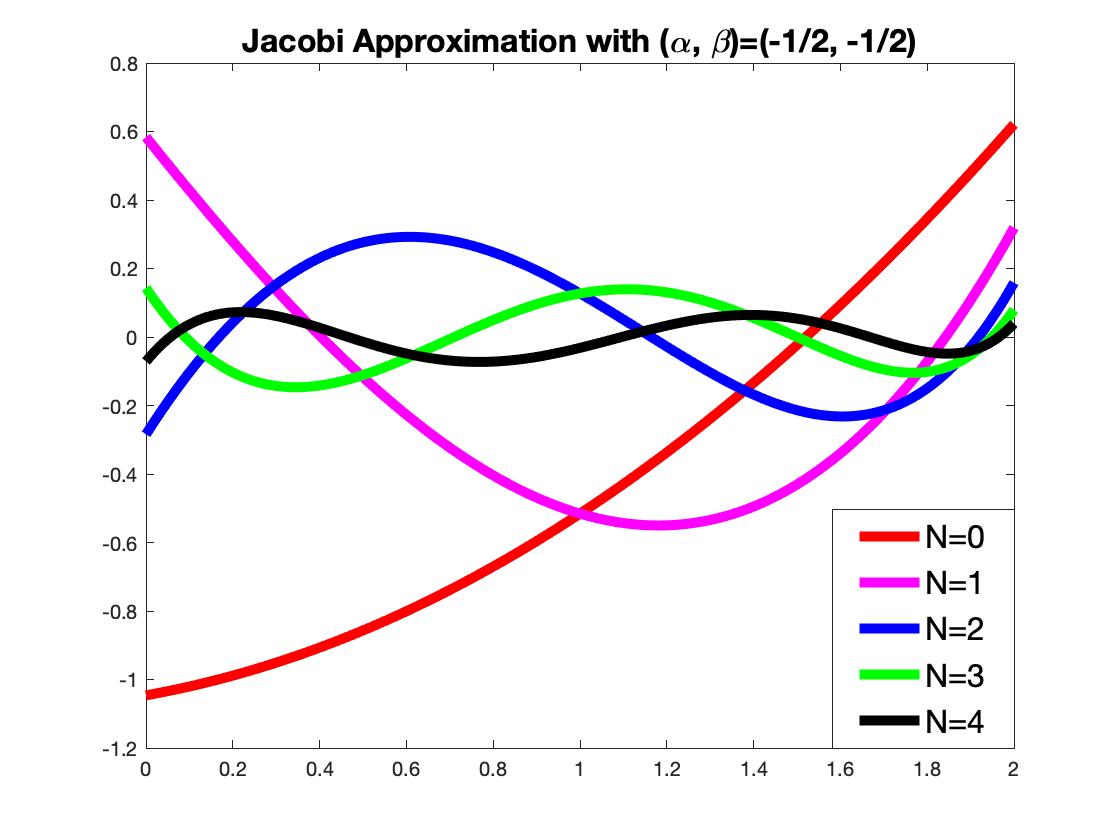
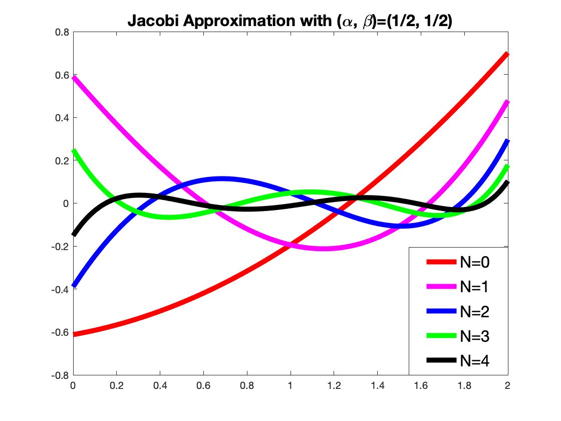
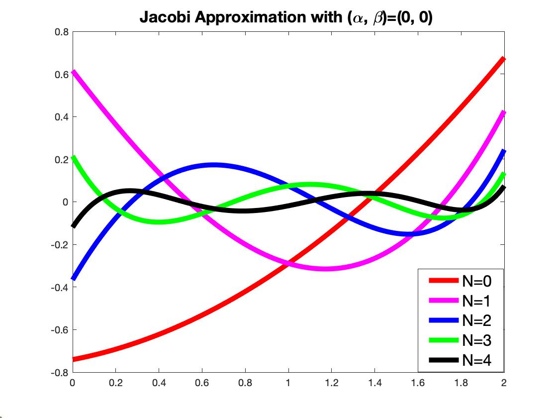
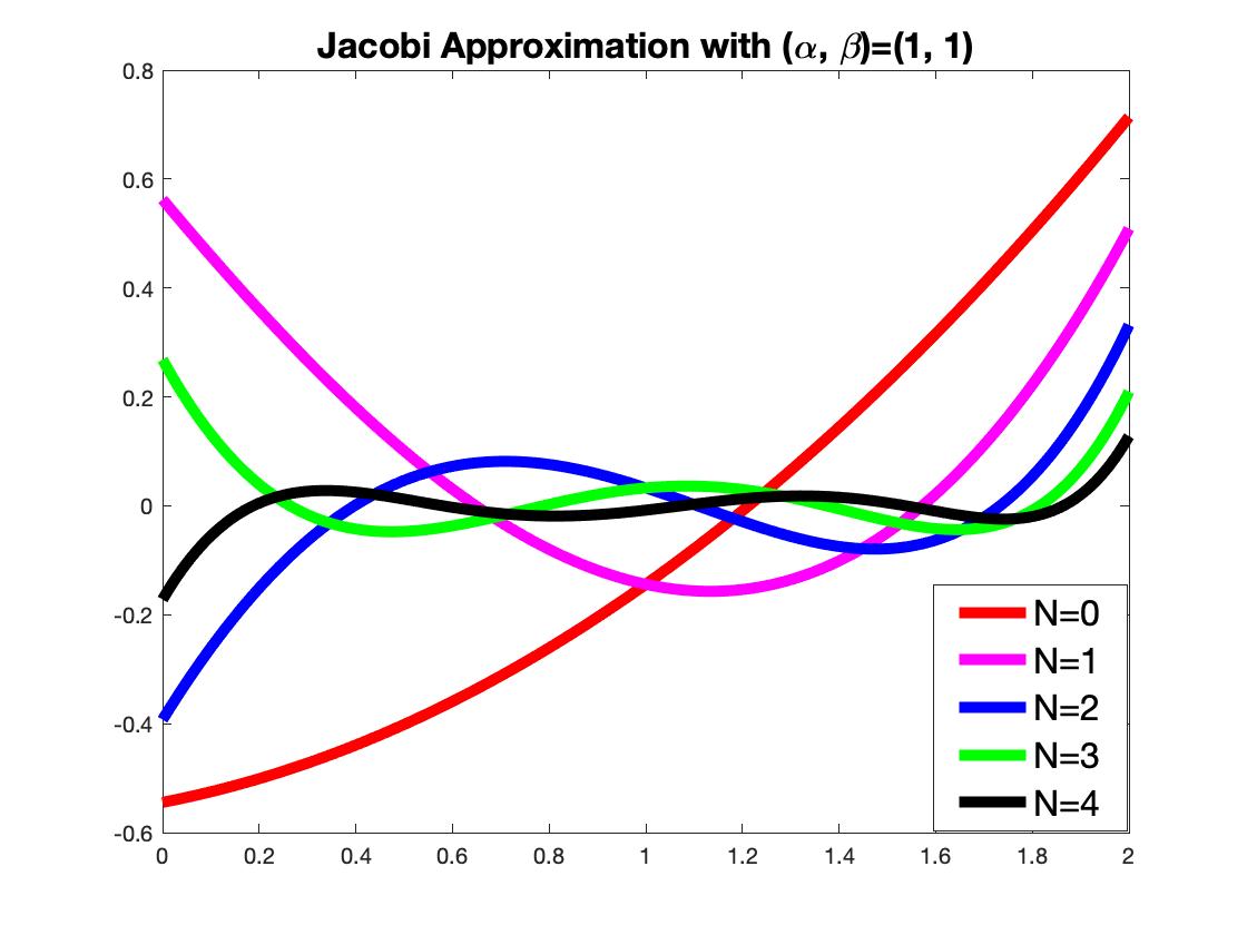
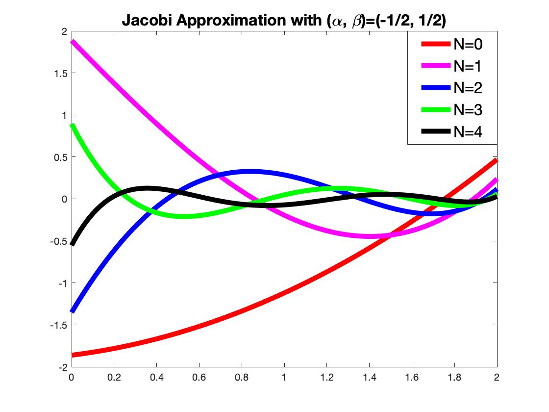
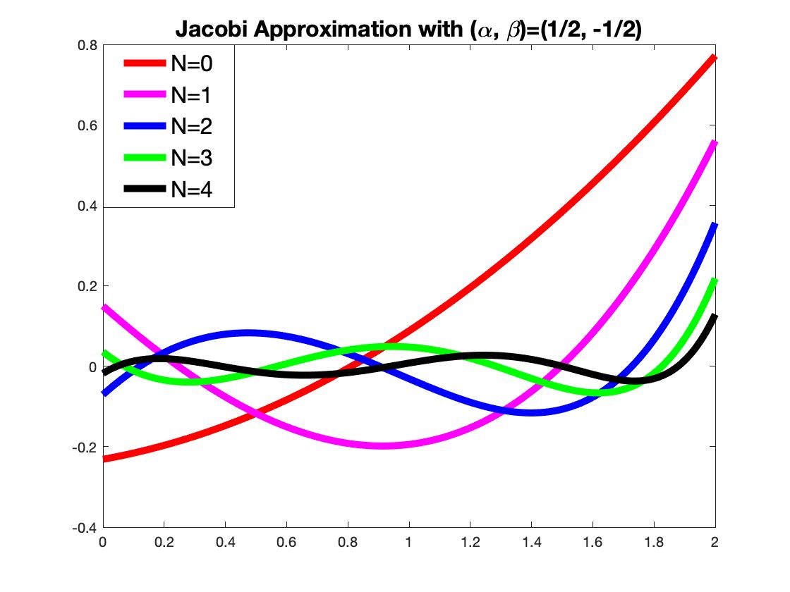
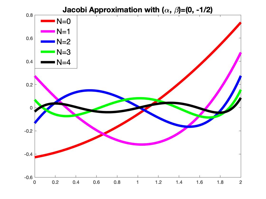
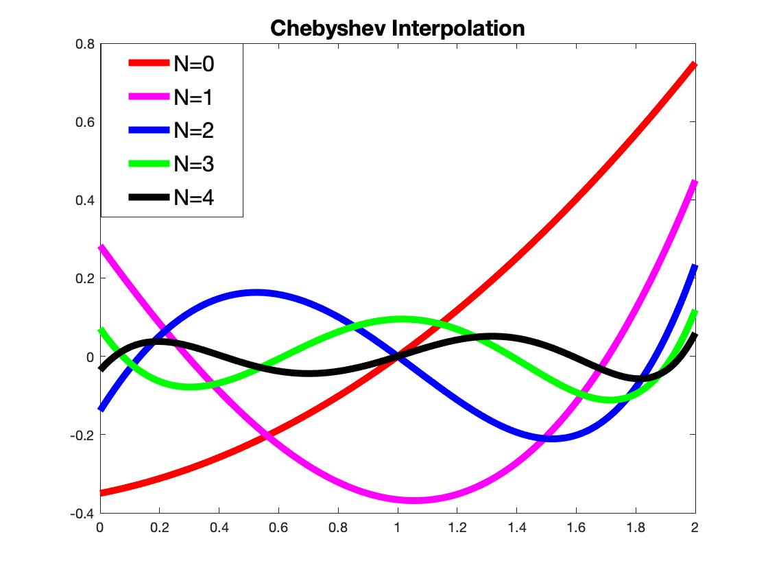
Figure 1: Plotted on the top three rows and the left of bottom row are the approximation error functions $1-h_{1}(t)g_{M}^{(\alpha,\beta)}(t),t\in[0,2],0\leq M\leq 4$ for pairs $(\alpha,\beta)=(-1/2,-1/2)$ (top row left), $(1/2,1/2)$ (top row right), $(0,0)$ (second row left), $(1,1)$ (second row right), $(-1/2,1/2)$ (third row left), $(1/2,-1/2)$ (third row right) and $(0,-1/2)$ (bottom row left). On the bottom row right is the approximation error function $1-h_{1}(t)C_{M}(t),t\in[0,2],0\leq M\leq 4$, between the Chebyshev interpolation polynomial $C_{M}(t)$ and the reciprocal of the polynomial $h_{1}(t)$.

TABLE I: Shown in the first seven rows are the maximal approximation error $b_{M}^{(\alpha,\beta)},0\leq M\leq 4$, of Jacobi polynomial approximations to $1/h_{1}$ on $[0,2]$, while in the last row is the maximal approximation error $\tilde{b}_{M},0\leq M\leq 4$, of Chebyshev interpolation approximation to $1/h_{1}$ on $[0,2]$.

	0	1	2	3	4
(-.5, -.5)	1.0463	0.5837	0.2924	0.1467	0.0728
(.5 .5)	0.7014	0.5904	0.3897	0.2505	0.1517
(0, 0)	0.7409	0.6153	0.3667	0.2146	0.1202
(1, 1)	0.7140	0.5626	0.3927	0.2686	0.1720
(-.5, .5)	1.8612	1.8855	1.3522	0.8937	0.5534
(.5, -.5)	0.7720	0.5603	0.3563	0.2184	0.1289
(0, -.5)	0.7356	0.4760	0.2749	0.1548	0.0850
ChebyInt	0.7500	0.4497	0.2342	0.1186	0.0595

Another excellent method of approximating the reciprocal of the polynomial $h$ on the cube $[{\boldsymbol{\mu}},{\bf\boldsymbol{\nu}}]$ is polynomial interpolation

$$C_{M}({\bf t})=\sum_{\|{\bf n}\|_{\infty}\leq M}d_{\bf n}{\bf t}^{\bf n}$$ (2.6)

at rescaled Chebyshev points ${\bf t}_{{\bf j};{\boldsymbol{\mu}},{\boldsymbol{\nu}}}=({t}_{j_{1},M},\ldots,{t}_{j_{d},M})$, i.e.,

$$C_{M}({\bf t}_{{\bf j};{\boldsymbol{\mu}},{\boldsymbol{\nu}}})=1/h({\bf t}_{{\bf j};{\boldsymbol{\mu}},{\boldsymbol{\nu}}}),$$ (2.7)

where

$${t}_{j_{k},M}=\frac{\nu_{k}+\mu_{k}}{2}+\frac{\nu_{k}-\mu_{k}}{2}\cos\frac{(j_{k}-1/2)\pi}{M+1}$$

for $1\leq j_{k}\leq M+1,1\leq k\leq d$. Recall that the Lebesgue constant for the above polynomial interpolation at rescaled Chebyshev points is of the order $(\ln(M+2))^{d}$. This together with the exponential convergence of Chebyshev polynomial approximation, see [41, Theorem 8.2] and [43, Theorem 2.2], implies that

$$\tilde{b}_{M}:=\sup_{{\bf t}\in[{\boldsymbol{\mu}},{\boldsymbol{\nu}}]}|1-h({\bf t})C_{M}({\bf t})|\leq D_{1}r_{1}^{M},\ M\geq 0,$$ (2.8)

for some positive constants $D_{1}\in(0,\infty)$ and $r_{1}\in(0,1)$. Shown in the bottom right of Figure 1 is our numerical demonstration to the above approximation property of the Chebyshev interpolation polynomial $C_{M}$, ChebyInt for abbreviation, to the function $1/h_{1}$, see bottom row of Table I for the maximal approximation error $\tilde{b}_{M},0\leq M\leq 4$, in (2.8) and also the numerical simulations in Section 6-A.

3 Polynomial approximation algorithm for inverse filtering

Let ${\mathbf{S}}_{1},\ldots,{\bf S}_{d}$ be commutative graph shifts whose joint spectrum $\Lambda$ in (1.4) is contained in a cube $[{\boldsymbol{\mu}},{\boldsymbol{\nu}}]$, i.e., (1.5) holds. The joint spectrum $\Lambda$ of commutative graph shifts ${\bf S}_{1},\ldots,{\bf S}_{d}$ plays a critical role in [15] to construct optimal/Chebyshev polynomial approximation to the inverse of a polynomial filter. In this section, based on the exponential approximation property of Jacobi polynomials and Chebyshev interpolation polynomials to the reciprocal of a nonvanishing multivariate polynomial, we propose an iterative Jacobi polynomial approximation algorithm and Chebyshev interpolation approximation algorithm to implement the inverse filtering procedure associated with a polynomial graph filter at the vertex level with one-hop communication.

Let $\alpha,\beta>-1$, $h$ be a multivariate polynomial satisfying (2.1), and let $g_{M}^{(\alpha,\beta)}$ and $C_{M},M\geq 0$, be the Jacobi polynomial approximation and Chebyshev interpolation polynomial approximation to $1/h$ in (2.3) and (2.7) respectively. Set ${\bf H}=h({\bf S}_{1},\ldots,{\bf S}_{d})$, ${\bf G}_{M}^{(\alpha,\beta)}=g_{M}^{(\alpha,\beta)}({\bf S}_{1},\ldots,{\bf S}_{d})$ and ${\bf C}_{M}=C_{M}({\bf S}_{1},\ldots,{\bf S}_{d}),M\geq 0$. By the spectral assumption (1.5), the spectral radii of ${\bf I}-{\bf G}_{M}^{(\alpha,\beta)}{\bf H}$ and ${\bf I}-{\bf C}_{M}{\bf H}$ are bounded by $b_{M}^{(\alpha,\beta)}$ in (2.4) and $\tilde{b}_{M}$ in (2.8) respectively, i.e.,

$$\rho({\bf I}-{\bf G}_{M}^{(\alpha,\beta)}{\bf H})\leq b^{(\alpha,\beta)}_{M}\ {\rm and}\ \rho({\bf I}-{\bf C}_{M}{\bf H})\leq\tilde{b}_{M},\ M\geq 0.$$ (3.1)

Therefore with appropriate selection of the polynomial degree $M$, applying the arguments used in [15, Theorem 3.1], we obtain the exponential convergence of the following iterative algorithm for inverse filtering,

$$\left\{\begin{array}[]{l}{\bf e}^{(m)}={\bf H}{\bf x}^{(m-1)}-{\bf y}\\ {\bf x}^{(m)}={\bf x}^{(m-1)}-{\bf G}_{M}{\bf e}^{(m)},\ m\geq 1\end{array}\right.$$ (3.2)

with arbitrary initials ${\bf x}^{(0)}$, where ${\bf G}_{M}$ is either ${\bf G}_{M}^{(\alpha,\beta)}$ or ${\bf C}_{M}$, and the input ${\bf y}$ of the inverse filtering procedure is obtained via the filtering procedure (1.1).

Theorem 3.1.

Let ${\mathbf{S}}_{1},\ldots,{\bf S}_{d}$ be commutative graph shifts satisfying (1.5), $h$ be a multivariate polynomial satisfying (2.1), and let $b_{M}^{(\alpha,\beta)}$ and $\tilde{b}_{M}$ be given in (2.4) and (2.8) respectively. If

$$b_{M}^{(\alpha,\beta)}<1\ \ ({\rm resp.}\ \tilde{b}_{M}<1),$$ (3.3)

then for any input ${\bf y}$, the sequence ${\bf x}^{(m)},m\geq 0$, in the iterative algorithm (3.2) with ${\bf G}_{M}={\bf G}_{M}^{(\alpha,\beta)}$ (resp. ${\bf G}_{M}={\bf C}_{M}$) converges to the output ${\bf H}^{-1}{\bf y}$ of the inverse filtering procedure (1.7) exponentially. In particular, there exist constants $C\in(0,\infty)$ and $r\in(\rho({\bf I}-{\bf G}_{M}^{(\alpha,\beta)}{\bf H}),1)$ (resp. $r\in(\rho({\bf I}-{\bf C}_{M}{\bf H}),1)$) such that

$$\|{\bf x}^{(m)}-{\bf H}^{-1}{\bf y}\|_{2}\leq C\|{\bf y}\|_{2}r^{m},\ m\geq 0.$$ (3.4)

We call the algorithm (3.2) with ${\bf G}_{M}={\bf G}_{M}^{(\alpha,\beta)}$ as Jacobi polynomial approximation algorithm, JPA$(\alpha,\beta)$ for abbreviation, and the iterative algorithm (3.2) with ${\bf G}_{M}={\bf C}_{M}$ as Chebyshev interpolation polynomial approximation algorithm, CIPA for abbreviation. By Theorem 3.1, the exponential convergence rates of the JPA$(\alpha,\beta)$ and CIPA are $\rho({\bf I}-{\bf G}_{M}^{(\alpha,\beta)}{\bf H})$ and $\rho({\bf I}-{\bf C}_{M}{\bf H})$ respectively. In addition to the exponential convergence, each iteration in the JPA$(\alpha,\beta)$ and CIPA contains essentially two filtering procedures associated with polynomial filters ${\bf G}_{M}$ and ${\bf H}$, and hence it can be implemented at the vertex level with one-hop communication, see [15, Algorithm 4]. Therefore the JPA$(\alpha,\beta)$ and CIPA algorithms can be implemented on a network with each agent equipped with limited storage and data processing ability, and one-hop communication subsystem. More importantly, the memory, computational cost and communication expense for each agent of the network are independent on the size of the whole network.

Remark 3.2.

We remark that the JPA$(\alpha,\beta)$ with $\alpha=\beta=-1/2$ was introduced in [15] as iterative Chebyshev polynomial approximation algorithm. For a positive definite polynomial filter ${\bf H}$, replacing the approximation filter ${\bf G}_{M}$ in the quasi-Newton algorithm (3.2) by $\gamma_{\rm opt}{\bf I}$, we obtain the traditional gradient descent method

$${\bf x}^{(m)}={\bf x}^{(m-1)}-\gamma_{\rm opt}({\bf H}{\bf x}^{(m-1)}-{\bf y}),\ m\geq 1$$ (3.5)

with the optimal step size $\gamma_{\rm opt}={2}/{(\lambda_{\min}({\bf H})+\lambda_{\rm max}({\bf H})})$, where $\lambda_{\max}({\bf H})$ and $\lambda_{\min}({\bf H})$ are the maximal and minimal eigenvalue of the matrix ${\bf H}$ respectively [18, 20, 21, 28, 29, 37, 38]. Numerical comparisons with the JPA$(\alpha,\beta)$ and CIPA algorithms to implement inverse filtering on circulant graphs will be given in Section 6-A.

4 Wiener filters for stationary graph signals

Let ${\mathbf{S}}_{1},\ldots,{\mathbf{S}}_{d}$ be real commutative symmetric graph shifts on a simple graph ${\mathcal{G}}=(V,E)$ of order $N\geq 1$ and assume that their joint spectrum is contained in some cube $[{\boldsymbol{\mu}},{\boldsymbol{\nu}}]$, i.e., (1.5) holds. In this section, we consider the scenario that the filtering procedure (1.1) has the filter

$${\bf H}=h({\mathbf{S}}_{1},\ldots,{\bf S}_{d})$$ (4.1a)

being a polynomial filter of $${\bf S}_{1},\ldots,{\bf S}_{d} {\bf x}$$, the inputs are stationary signals with the correlation matrix

$${\bf R}=r({\mathbf{S}}_{1},\ldots,{\mathbf{S}}_{d})$$ (4.1b)

being a polynomial of graph shifts $${\bf S}_{1},\ldots,{\mathbf{S}}_{d}$$ ([34, 35, 36]), and the outputs

$${\bf y}={\bf H}{\bf x}+{\boldsymbol{\epsilon}}$$ (4.1c)

are corrupted by some random noise $${\boldsymbol{\epsilon}} {\bf x} {\bf G} {\bf S}_{1},\ldots,{\mathbf{S}}_{d}$$ being independent with the input signal , and having zero mean and covariance matrix to be a polynomial of graph shifts , i.e.,

$${\mathbb{E}}{\boldsymbol{\epsilon}}={\bf 0},\ {\mathbb{E}}{\boldsymbol{\epsilon}}{\bf x}^{T}={\bf 0}\ {\rm and}\ {\bf G}=g({\bf S}_{1},\ldots,{\bf S}_{d})$$ (4.1d)

for some multivariate polynomial $g$. In this section, we find the optimal reconstruction filter ${\bf W}_{\rm mse}$ with respect to the stochastic mean squared error $F_{{\rm mse},P,{\bf K}}$ in (4.3), and we propose a distributed algorithm to implement the stochastic Wiener filtering procedure ${\bf y}\longmapsto{\bf W}_{\rm mse}{\bf y}$ at the vertex level with one-hop communication. In this section, we also consider optimal unbiased reconstruction filters for the scenario that the input signals ${\bf x}$ are wide-band stationary, i.e.,

$${\mathbb{E}}{\bf x}=c{\bf 1}\ \ {\rm and}\ \ {\mathbb{E}}({\bf x}-{\mathbb{E}}{\bf x})({\bf x}-{\mathbb{E}}({\bf x}))^{T}=\widetilde{\bf R}=\tilde{r}({\bf S}_{1},\ldots,{\bf S}_{d}),$$ (4.2)

for some $0\neq c\in{\mathbb{R}}$ and some multivariate polynomial $\tilde{r}$, The concept of (wide-band) stationary signals was introduced in [34, Definition 3] in which the graph Laplacian is used as the graph shift.

For a probability measure $P=(p(i))_{i\in V}$ on the graph ${\mathcal{G}}$ and a regularization matrix ${\bf K}$, we define the stochastic mean squared error of a reconstruction filter ${\bf W}$ by

$$F_{{\rm mse},P,{\bf K}}({\bf W})={\mathbb{E}}({\bf W}{\bf y}-{\bf x})^{T}{\bf P}({\bf W}{\bf y}-{\bf x})+{\bf y}^{T}{\bf W}^{T}{\bf K}{\bf W}{\bf y},$$ (4.3)

where ${\bf P}$ is the diagonal matrix with diagonal entries $p(i),i\in V$. The stochastic mean squared error $F_{{\rm mse},P,{\bf K}}({\bf W})$ in (4.3) contains the regularization term ${\mathbb{E}}{\bf y}^{T}{\bf W}^{T}{\bf K}{\bf W}{\bf y}$ and the fidelity term ${\mathbb{E}}({\bf W}{\bf y}-{\bf x})^{T}{\bf P}({\bf W}{\bf y}-{\bf x})=\sum_{i\in V}p(i){\mathbb{E}}|({\bf W}{\bf y})(i)-{x}(i)|^{2}$. It is discussed in [34] for the case that the filter ${\bf H}$, the covariance ${\bf G}$ of noises and the regularizer ${\bf K}$ are polynomials of the graph Laplacian ${\bf L}$, and that the probability measure $P$ is the uniform probability measure $P_{U}$, i.e., $p_{U}(i)=1/N,i\in V$. In the following theorem, we provide an explicit solution to the minimization $\min_{\bf W}F_{{\rm mse},P,{\bf K}}({\bf W})$, see Appendix A for the proof.

Theorem 4.1.

Let the filter ${\bf H}$, the input signal ${\bf x}$, the noisy output signal ${\bf y}$ and additive noise ${\boldsymbol{\epsilon}}$ be as in (4.1), and let the stochastic mean squared error $F_{{\rm mes},P,{\bf K}}$ be as in (4.3). Assume that ${\bf H}{\bf R}{\bf H}^{T}+{\bf G}$ and ${\bf P}+{\bf K}$ are strictly positive definite, and define

$${\bf W}_{{\rm mse}}=({\bf P}+{\bf K})^{-1}{\bf P}{\bf R}{\bf H}^{T}\big{(}{\bf H}{\bf R}{\bf H}^{T}+{\bf G})^{-1}.$$ (4.4)

Then ${\bf W}_{{\rm mse}}$ is the unique minimizer of the minimization problem

$${\bf W}_{{\rm mse}}=\arg\min_{\bf W}F_{{\rm mse},P,{\bf K}}({\bf W}),$$ (4.5)

and

$$F_{{\rm mse},P,{\bf K}}({\bf W}_{\rm mse})={\rm tr}\big{(}{\bf P}({\bf I}-{\bf W}_{\rm mse}{\bf H}\big{)}{\bf R}\big{)}.$$ (4.6)

We call the optimal reconstruction filter ${\bf W}_{\rm mse}$ in (4.4) as the stochastic Wiener filter. For the case that the stochastic mean squared error does not take the regularization term into account, i.e., ${\bf K}={\bf 0}$, we obtain from (4.4) that the corresponding stochastic Wiener filter ${\bf W}_{\rm mse}$ becomes

$${\bf W}_{\rm mse}^{0}={\bf R}{\bf H}^{T}\big{(}{\bf H}{\bf R}{\bf H}^{T}+{\bf G})^{-1},$$ (4.7)

which is independent of the probability measure $P=(p(i))_{i\in V}$ on the graph ${\mathcal{G}}$. If we further assume that the probability measure $P$ is the uniform probability measure $P_{U}$ and the input signals ${\bf x}$ are i.i.d with mean zero and variance $\delta_{1}$, the stochastic Wiener filter becomes

$${\bf W}_{\rm mse}^{0}=\delta_{1}^{2}{\bf H}^{T}(\delta_{1}^{2}{\bf H}{\bf H}^{T}+{\bf G})^{-1}$$

and the corresponding stochastic mean squared error is given by

$$F_{{\rm mes},P_{U}}({\bf W}_{\rm mse}^{0})=\frac{\delta_{1}^{2}}{N}{\rm tr}\left((\delta_{1}^{2}{\bf H}{\bf H}^{T}+{\bf G})^{-1}{\bf G}\right),$$ (4.8)

cf. (5.7) and (5.8), and [34, Eqn. 16].

Denote the reconstructed signal via the stochastic Wiener filter ${\bf W}_{\rm mse}$ by

$${\bf x}_{\rm mse}={\bf W}_{\rm mse}{\bf y},$$ (4.9)

where ${\bf y}$ is given in (4.1c). The above estimator via stochastic Wiener filter ${\bf W}_{\rm mse}$ is biased in general. For the case that ${\bf G},{\bf H},{\bf K}$ and ${\bf R}$ are polynomials of commutative symmetric graph shifts ${\mathbf{S}}_{1},\ldots,{\mathbf{S}}_{d}$, one may verify that matrices ${\bf H}^{T},{\bf H},{\bf G},{\bf R},{\bf K}$ are commutative, and

$${\mathbb{E}}({\bf x}-{\bf x}_{\rm mse}) \hskip-5.78172pt= \hskip-5.78172pt({\bf P}+{\bf K})^{-1}\big{(}{\bf H}{\bf R}{\bf H}^{T}+{\bf G})^{-1}{\bf R}{\bf H}^{T}{\bf H}{\bf K}{\mathbb{E}}{\bf x}$$ (4.10)

$$\hskip-5.78172pt+\big{(}{\bf H}{\bf R}{\bf H}^{T}+{\bf G})^{-1}{\bf G}{\mathbb{E}}{\bf x}.$$

Therefore the estimator (4.9) is unbiased if

$${\mathbf{K}}{\mathbb{E}}{\bf x}={\mathbf{G}}{\mathbb{E}}{\bf x}={\bf 0}.$$ (4.11)

Remark 4.2.

By (4.4) and (4.7), the reconstructed signal ${\bf x}_{\rm mse}$ in (4.9) can be obtained in two steps,

$${\bf w}={\bf W}_{\rm mse}^{0}{\bf y}={\bf R}{\bf H}^{T}\big{(}{\bf H}{\bf R}{\bf H}^{T}+{\bf G}\big{)}^{-1}{\bf y},$$ (4.12a)

and

$${\bf x}_{\rm mse}={\bf P}^{-1/2}\big{(}{\bf I}+{\bf P}^{-1/2}{\bf K}{\bf P}^{-1/2})^{-1}{\bf P}^{1/2}{\bf w},$$ (4.12b)

where the first step (4.12a) is the Wiener filtering procedure without the regularization term taken into account, and the second step (4.12b) is the solution of the following Tikhonov regularization problem,

$${\bf x}_{\rm mse}=\arg\min_{\bf x}\ ({\bf x}-{\bf w})^{T}{\bf P}({\bf x}-{\bf w})+{\bf x}^{T}{\bf K}{\bf x}.$$ (4.13)

By symmetry and commutativity assumptions on the graph shifts ${\mathbf{S}}_{1},\ldots,{\mathbf{S}}_{d}$, and the polynomial assumptions (4.1a), (4.1b) and (4.1d), the Wiener filter ${\bf W}_{\rm mse}^{0}$ in (4.7) is the product of a polynomial filter ${\bf R}{\bf H}^{T}=(hr)({\mathbf{S}}_{1},\ldots,{\mathbf{S}}_{d})$ and the inverse of another polynomial filter ${\bf H}{\bf R}{\bf H}^{T}+{\bf G}=(h^{2}r+g)({\mathbf{S}}_{1},\ldots,{\bf S}_{d})$. Set ${\bf z}_{1}=({\bf H}{\bf R}{\bf H}^{T}+{\bf G})^{-1}{\bf y}$. Therefore using [15, Algorithms 1 and 2], the filtering procedure ${\bf w}={\bf R}{\bf H}^{T}{\bf z}_{1}$ can be implemented at the vertex level with one-hop communication. Also we observe that the Jacobi polynomial approximation algorithm and Chebyshev interpolation polynomial approximation algorithm in Section 3 can be applied to the inverse filtering procedure ${\bf y}\longmapsto{\bf z}_{1}$, when

$$h^{2}({\bf t})r({\bf t})+g({\bf t})>0\ {\rm for\ all}\ {\bf t}\in[{\boldsymbol{\mu}},{\boldsymbol{\nu}}],$$ (4.14)

see Part I of Algorithm 4.1 for the implementation of the Wiener filtering procedure (4.12a) without regularization at the vertex level.

Set ${\bf z}_{2}={\bf P}^{1/2}{\bf w}$ and ${\bf z}_{3}=\big{(}{\bf I}+{\bf P}^{-1/2}{\bf K}{\bf P}^{-1/2})^{-1}{\bf z}_{2}$. As ${\bf P}$ is a diagonal matrix, the rescaling procedure ${\bf z}_{2}={\bf P}^{1/2}{\bf w}$ and ${\bf x}_{\rm mse}={\bf P}^{-1/2}{\bf z}_{3}$ can be implemented at the vertex level. Then it remains to find a distributed algorithm to implement the inverse filtering procedure

$${\bf z}_{3}=\big{(}{\bf I}+{\bf P}^{-1/2}{\bf K}{\bf P}^{-1/2})^{-1}{\bf z}_{2}$$ (4.15)

at the vertex level. As ${\bf P}^{-1/2}$ may not commutate with the graph shifts ${\bf S}_{1},\ldots,{\bf S}_{d}$, the filter ${\bf I}+{\bf P}^{-1/2}{\bf K}{\bf P}^{-1/2}$ is not necessarily a polynomial filter of some commutative graph shifts even if ${\bf K}=k({\bf S}_{1},\ldots,{\bf S}_{d})$ is, hence the polynomial approximation algorithm proposed in Section 3 does not apply to the above inverse filtering procedure directly.

Next we propose a novel exponentially convergent algorithm to implement the inverse filtering procedure (4.15) at the vertex level when the positive semidefinite regularization matrix ${\bf K}=k({\bf S}_{1},\ldots,{\bf S}_{d})$ is a polynomial of graph shifts ${\bf S}_{1},\ldots,{\bf S}_{d}$. Set

$$K=\sup_{{\bf t}\in[{\boldsymbol{\mu}},{\boldsymbol{\nu}}]}k({\bf t})\ {\rm and}\ p_{\min}=\min_{i\in V}p(i).$$

Then one may verify that

$${\bf I}\preceq{\bf I}+{\bf P}^{-1/2}{\bf K}{\bf P}^{-1/2}\preceq\frac{K+p_{\min}}{p_{\min}}{\bf I},$$ (4.16)

where for symmetric matrices ${\bf A}$ and ${\bf B}$, we use ${\bf A}\preceq{\bf B}$ to denote the positive semidefiniteness of ${\bf B}-{\bf A}$. Applying Neumann series expansion $(1-t)^{-1}=\sum_{n=0}^{\infty}t^{n}$ with $t$ replaced by ${\bf I}-\frac{p_{\min}}{K+p_{\min}}({\bf I}+{\bf P}^{-1/2}{\bf K}{\bf P}^{-1/2})$, we obtain

$$\hskip-5.78172pt\big{(}{\bf I}+{\bf P}^{-1/2}{\bf K}{\bf P}^{-1/2})^{-1}$$

$$\hskip-5.78172pt= \hskip-5.78172pt\frac{p_{\min}}{K+p_{\min}}\sum_{n=0}^{\infty}\left(\frac{K{\bf I}-p_{\min}{\bf P}^{-1/2}{\bf K}{\bf P}^{-1/2}}{K+p_{\min}}\right)^{n}.\qquad$$

Therefore the sequence ${\bf w}_{m},m\geq 0$, defined by

$${\bf w}_{m+1} \hskip-5.78172pt= \hskip-5.78172pt\frac{p_{\min}}{K+p_{\min}}{\bf w}_{0}+\frac{K}{K+p_{\min}}{\bf w}_{m}$$ (4.17)

$$\hskip-5.78172pt-\frac{p_{\min}}{K+p_{\min}}{\bf P}^{-1/2}{\bf K}{\bf P}^{-1/2}{\bf w}_{m},\ m\geq 0\quad$$

with initial ${\bf w}_{0}={\bf z}_{2}$ converges to ${\bf z}_{3}$ exponentially, since

$$\hskip-5.78172pt\|{\bf w}_{m}-{\bf z}_{3}\|_{2}$$

$$\hskip-5.78172pt= \hskip-5.78172pt\frac{p_{\min}}{K+p_{\min}}\left\|\sum_{n=m+1}^{\infty}\left(\frac{K{\bf I}-p_{\min}{\bf P}^{-1/2}{\bf K}{\bf P}^{-1/2}}{K+p_{\min}}\right)^{n}{\bf z}_{2}\right\|_{2}$$

$$\hskip-5.78172pt\leq \hskip-5.78172pt\frac{p_{\min}\|{\bf z}_{2}\|_{2}}{K+p_{\min}}\sum_{n=m+1}^{\infty}\left\|\frac{K{\bf I}-p_{\min}{\bf P}^{-1/2}{\bf K}{\bf P}^{-1/2}}{K+p_{\min}}\right\|^{n}$$

$$\hskip-5.78172pt\leq \hskip-5.78172pt\frac{p_{\min}\|{\bf z}_{2}\|_{2}}{K+p_{\min}}\sum_{n=m+1}^{\infty}\left(\frac{K}{K+p_{\min}}\right)^{n}$$

$$\hskip-5.78172pt= \hskip-5.78172pt\left(\frac{K}{K+p_{\min}}\right)^{m+1}\|{\bf z}_{2}\|_{2},\ m\geq 1,$$

where the last inequality follows from (4.16). More importantly, each iteration in the algorithm to implement the inverse filtering procedure (4.15) contains mainly two rescaling procedure and a filter procedure associated with the polynomial filter ${\bf K}$ which can be implemented by [15, Algorithms 1 and 2]. Hence the regularization procedure (4.12b) can be implemented at the vertex level with one-hop communication, see Part 2 of Algorithm 4.1.

Algorithm 4.1 Polynomial approximation algorithm to implement the Wiener filtering procedure ${\bf x}_{\rm mse}={\bf W}_{\rm mse}{\bf y}$ at a vertex $i\in V$.

  Inputs: Polynomial coefficients of polynomial filters ${\bf H},{\bf G},{\bf K},{\bf R}$ and ${\bf G}_{M}$ (either Jacobi polynomial approximation filter ${\bf G}_{M}^{(\alpha,\beta)}$ or Chebyshev interpolation approximation filter ${\bf C}_{M}$ to the inverse filter $({\bf H}^{2}{\bf R}+{\bf G})^{-1}$), entries $S_{k}(i,j),j\in{\mathcal{N}}_{i}$ in the $i$-th row of the shifts ${\bf S}_{k},1\leq k\leq d$, the value $y(i)$ of the input signal ${\bf y}=(y(i))_{i\in V}$ at the vertex $i$, the probability $p(i)$ at the vertex $i$, and numbers $L_{1}$ and $L_{2}$ of the first and second iteration.

  Part I:  Implementation of the Wiener filtering procedure (4.12a) at the vertex $i$

  Pre-processing:  Find the polynomial coefficients of polynomial filters ${\bf H}^{2}{\bf R}+{\bf G}$ and ${\bf R}{\bf H}$.

  Initialization:  $n=0$ and zero initial $x^{(0)}(i)=0$.

  Iteration:  Use [15, Algorithms 1 and 2] to implement the filtering procedures ${\bf e}^{(m)}=({\bf H}{\bf R}{\bf H}^{T}+{\bf G}){\bf x}^{(m-1)}-{\bf y}$ and ${\bf x}^{(m)}={\bf x}^{(m-1)}-{\bf G}_{M}{\bf e}^{(m)},0\leq m\leq L_{1}$ at the vertex $i$.

  Output of the iteration:  Denote the output of the $L_{1}$-th iteration by $z_{1}^{(L_{1})}(i)$, which is the approximate value of the output data of the inverse filtering procedure ${\bf z}_{1}=({\bf H}^{2}{\bf R}+{\bf G})^{-1}{\bf y}$ at the vertex $i$.

  Post-processing after the iteration: Use [15, Algorithms 1 and 2] to implement the filtering procedure ${\bf w}={\bf R}{\bf H}{\bf z}_{1}={\bf W}_{\rm mse}^{0}{\bf y}$ at the vertex $i$, where the input is $z_{1}^{(L_{1})}(i)$ and the output denoted by $w^{(L_{1})}(i)$, is the approximate value of the output data of the above filtering procedure.

  Part II:  Implementation of the regularization procedure (4.12b) at the vertex $i$

  Pre-processing:  Rescaling $z_{2}^{(L_{1})}(i)=p(i)^{1/2}w^{(L_{1})}(i)$, the approximate value of the output data of the rescaling procedure ${\bf z}_{2}={\bf P}^{1/2}{\bf w}$.

  Iteration:  Start from ${\bf w}_{0}(i)=z_{2}^{(L_{1})}(i)$, and use [15, Algorithms 1 and 2] and rescaling ${\bf P}^{-1/2}$ to implement the procedure (4.17) for $0\leq m\leq L_{2}$, with the output, denoted by $z_{3}^{(L_{1},L_{2})}(i)$, being the approximation value of the output data of the inverse filtering procedure ${\bf z}_{3}=\big{(}{\bf I}+{\bf P}^{-1/2}{\bf K}{\bf P}^{-1/2})^{-1}{\bf z}_{2}$ at the vertex $i$

  Post-processing: ${x}_{\rm mse}^{(L_{1},L_{2})}(i)=p(i)^{-1/2}z_{3}^{(L_{1},L_{2})}(i)$.

  Output: $x_{\rm mse}(i)\approx{x}_{\rm mse}^{(L_{1},L_{2})}(i)$, the approximate value of the output data of the Wiener filtering procedure ${\bf x}_{\rm mse}=({\bf P}+{\bf K})^{-1}{\bf P}{\bf w}={\bf W}_{\rm mse}{\bf y}$ at the vertex $i$.

Remark 4.3.

We remark that for the case that the probability measure $P$ is uniform [34], ${\bf I}+{\bf P}^{-1/2}{\bf K}{\bf P}^{-1/2}={\bf I}+N{\bf K}$ is a polynomial filter of ${\bf S}_{1},\ldots,{\bf S}_{d}$ if ${\bf K}=k({\bf S}_{1},\ldots,{\bf S}_{d})$ is, and hence JPA$(\alpha,\beta)$ and CIPA algorithms proposed in Section 3 can be applied to the inverse filtering procedure ${\bf z}_{3}=\big{(}{\bf I}+{\bf P}^{-1/2}{\bf K}{\bf P}^{-1/2})^{-1}{\bf z}_{2}$ if $1+Nk({\bf t})>0\ {\rm for\ all}\ {\bf t}\in[{\boldsymbol{\mu}},{\boldsymbol{\nu}}]$.

We finish this section with optimal unbiased Wiener filters for the scenario that the input signals ${\bf x}$ are wide-stationary, i.e., ${\bf x}$ satisfies (4.2), the filtering procedure satisfies (4.1a) and

$${\bf H}{\bf 1}=\tau{\bf 1}$$ (4.18)

for some $\tau\neq 0$, the output ${\bf y}$ in (4.1c) are corrupted by some noise ${\boldsymbol{\epsilon}}$ satisfying (4.1d), and the covariance matrix ${\bf G}$ of the noise and the regularization matrix ${\bf K}$ satisfy

$${\bf G}{\bf 1}={\bf K}{\bf 1}={\bf 0}.$$ (4.19)

In the above setting, the random variable $\tilde{\bf x}={\bf x}-{\mathbb{E}}{\bf x}={\bf x}-c{\bf 1}$ satisfies

$${\mathbb{E}}\tilde{\bf x}={\bf 0},{\mathbb{E}}{\tilde{\bf x}}{\boldsymbol{\epsilon}}^{T}={\bf 0}\ {\rm and}\ {\mathbb{E}}\tilde{\bf x}\tilde{\bf x}^{T}=\widetilde{\bf R}=\tilde{r}({\mathbf{S}}_{1},\ldots,{\mathbf{S}}_{d}).$$ (4.20)

For any unbiased reconstruction filter ${\bf W}$, we have

$${\bf W}{\bf H}{\bf 1}={\bf 1}.$$

This together with (4.19) implies that

$${\bf W}{\bf y}-{\bf x} \hskip-5.78172pt= \hskip-5.78172ptc({\bf W}{\bf H}{\bf 1}-{\bf 1})+({\bf W}{\bf H}-{\bf I})\tilde{\bf x}+{\bf W}{\boldsymbol{\epsilon}}$$

$$\hskip-5.78172pt= \hskip-5.78172pt({\bf W}{\bf H}-{\bf I})\tilde{\bf x}+{\bf W}{\boldsymbol{\epsilon}}$$

and

$${\bf y}^{T}{\bf W}^{T}{\bf K}{\bf W}{\bf y} \hskip-5.78172pt= \hskip-5.78172pt({\bf H}\tilde{\bf x}+{\boldsymbol{\epsilon}})^{T}{\bf W}^{T}{\bf K}{\bf W}({\bf H}\tilde{\bf x}+{\boldsymbol{\epsilon}})+{\bf 1}^{T}{\bf K}{\bf 1}$$

$$\hskip-5.78172pt+{\bf 1}^{T}{\bf K}{\bf W}({\bf H}\tilde{\bf x}+{\boldsymbol{\epsilon}})+({\bf H}\tilde{\bf x}+{\boldsymbol{\epsilon}})^{T}{\bf W}^{T}{\bf K}{\bf 1}$$

$$\hskip-5.78172pt= \hskip-5.78172pt({\bf H}\tilde{\bf x}+{\boldsymbol{\epsilon}})^{T}{\bf W}^{T}{\bf K}{\bf W}({\bf H}\tilde{\bf x}+{\boldsymbol{\epsilon}}).$$

Therefore following the argument used in the proof of Theorem 4.1 with the signal ${\bf x}$ and polynomial $r$ replaced by $\tilde{\bf x}$ and $\tilde{r}$ respectively, and applying (4.11), (4.18) and (4.20), we can show that the stochastic Wiener filter $\widetilde{\bf W}_{\rm mse}$ in (4.22) is an optimal unbiased filter to reconstruct wide-band stationary signals.

Theorem 4.4.

Let the input signal ${\bf x}$, the noisy output signal ${\bf y}$ and the additive noise ${\boldsymbol{\epsilon}}$ be in (4.2), (4.1c), (4.1d), the covariance matrix ${\bf G}$ of the noise and the regularization matrix ${\bf K}$ satisfy (4.19), and let the filtering procedure associated with the filter ${\bf H}$ satisfy (4.1a) and (4.18). Assume that ${\bf H}\widetilde{\bf R}{\bf H}^{T}+{\bf G}$ and ${\bf P}+{\bf K}$ are strictly positive definite. Then

$$F_{{\rm mse},P,{\bf K}}({\bf W})\geq F_{{\rm mse},P,{\bf K}}(\widetilde{\bf W}_{\rm mse})$$ (4.21)

hold for all unbiased reconstructing filters ${\bf W}$, where $F_{{\rm mse},P,{\bf K}}({\bf W})$ is the stochastic mean squared error in (4.3) and

$$\widetilde{\bf W}_{\rm mse}=({\bf P}+{\bf K})^{-1}{\bf P}\widetilde{\bf R}{\bf H}^{T}({\bf H}\widetilde{\bf R}{\bf H}^{T}+{\bf G})^{-1}.$$ (4.22)

Moreover, $\tilde{\bf x}_{\rm mse}=\widetilde{\bf W}_{\rm mse}{\bf y}$ is an unbiased estimator to the wide-band stationary signal ${\bf x}$.

Following the distributed algorithm used to implement the stochastic Wiener filtering procedure, the unbiased estimation $\tilde{\bf x}_{\rm mse}=\widetilde{\bf W}_{\rm mse}{\bf y}$ can be implemented at the vertex level with one-hop communication when

$$h^{2}({\bf t})\tilde{r}({\bf t})+g({\bf t})>0\ {\rm for\ all}\ {\bf t}\in[{\boldsymbol{\mu}},{\boldsymbol{\nu}}].$$

Numerical demonstrations to denoise wide-band stationary signals are presented in Section 6-C.

5 Wiener filters for deterministic graph signals

Let ${\mathbf{S}}_{1},\ldots,{\mathbf{S}}_{d}$ be real commutative symmetric graph shifts on a simple graph ${\mathcal{G}}=(V,E)$ and their joint spectrum be contained in some cube $[{\boldsymbol{\mu}},{\boldsymbol{\nu}}]$, i.e., (1.5) holds. In this section, we consider the scenario that the filtering procedure (1.1) has the filter ${\bf H}$ given in (4.1a), its inputs ${\bf x}=(x(i))_{i\in V}$ are deterministic signals with their energy bounded by some $\delta_{0}>0$,

$$\|{\bf x}\|_{2}\leq\delta_{0},$$ (5.1)

and its outputs

$${\bf y}={\bf H}{\bf x}+{\boldsymbol{\epsilon}}$$ (5.2)

are corrupted by some random noise ${\boldsymbol{\epsilon}}$ which has mean zero and covariance matrix ${\bf G}={\rm cov}({\boldsymbol{\epsilon}})$ being a polynomial of graph shifts ${\bf S}_{1},\ldots,{\mathbf{S}}_{d}$,

$${\mathbb{E}}{\boldsymbol{\epsilon}}={\bf 0}\ \ {\rm and}\ {\bf G}=g({\bf S}_{1},\ldots,{\bf S}_{d})$$ (5.3)

for some multivariate polynomial $g$. For the above setting of the filtering procedure, we introduce the worst-case mean squared error of a reconstruction filter ${\bf W}$ by

$$F_{{\rm wmse},P}({\bf W})=\sum_{i\in V}p(i)\max_{\|{\bf x}\|_{2}\leq\delta_{0}}{\mathbb{E}}|({\bf W}{\bf y})(i)-{x}(i)|^{2},$$ (5.4)

where $P=(p(i))_{i\in V}$ is a probability measure on the graph ${\mathcal{G}}$ [32, 44]. In this section, we discuss the optimal reconstruction filter ${\bf W}_{\rm wmse}$ with respect to the worst-case mean squared error $F_{{\rm wmse},P}$ in (5.4), and we propose a distributed algorithm to implement the worst-case Wiener filtering procedure at the vertex level with one-hop communication.

First, we provide a universal solution to the minimization problem

$$\min_{\bf W}F_{{\rm wmse},P}({\bf W}),$$ (5.5)

which is independent of the probability measure $P$, see Appendix B for the proof.

Theorem 5.1.

Let the filter ${\bf H}$, the input ${\bf x}$, the noisy output ${\bf y}$, the noise $\boldsymbol{\epsilon}$, and the worst-case mean squared error $F_{{\rm wmse},P}$ be as in (4.1a), (5.1), (5.2), (5.3) and (5.4) respectively. Assume that $\delta_{0}^{2}{\bf H}{\bf H}^{T}+{\bf G}$ is strictly positive definite. Then

$$F_{{\rm wmse},P}({\bf W}) \hskip-5.78172pt\geq \hskip-5.78172ptF_{{\rm wmse},P}({\bf W}_{\rm wmse})$$ (5.6)

$$\hskip-5.78172pt= \hskip-5.78172pt\delta_{0}^{2}-\delta_{0}^{4}{\rm tr}((\delta_{0}^{2}{\bf H}{\bf H}^{T}+{\bf G})^{-1}{\bf H}{\bf P}{\bf H}^{T}\big{)}\qquad$$

hold for all reconstructing filters ${\bf W}$, where ${\bf P}$ is the diagonal matrix with diagonal entries $p(i),i\in V$, and

$${\bf W}_{{\rm wmse}}=\delta_{0}^{2}{\bf H}^{T}\big{(}\delta_{0}^{2}{\bf H}{\bf H}^{T}+{\bf G})^{-1}.$$ (5.7)

Moreover, the reconstruction filter ${\bf W}_{\rm wmse}$ is the unique solution of the minimization problem (5.5) if ${\bf P}$ is invertible, i.e., the probability $p(i)$ at every vertex $i\in V$ is positive.

We call the optimal reconstruction error ${\bf W}_{\rm wmse}$ in (5.7) as the worst-case Wiener filter. Denote the order of the graph ${\mathcal{G}}$ by $N$. For the case that the probability measure $P$ is the uniform probability measure $P_{U}$, we can simplify the estimate (5.6) as follows:

$$F_{{\rm wmse},P_{U}}({\bf W}_{\rm wmse})=\frac{\delta_{0}^{2}}{N}{\rm tr}\big{(}(\delta_{0}^{2}{\bf H}{\bf H}^{T}+{\bf G})^{-1}{\bf G}\big{)},$$ (5.8)

c.f. (4.8). If the random noises ${\boldsymbol{\epsilon}}$ are further assumed to be i.i.d and have mean zero and variance $\sigma$, we can use singular values $\mu_{i}({\bf H}),1\leq i\leq N$, of the filter ${\bf H}$ to estimate the worst-case mean squared error for the worst-case Wiener filter ${\bf W}_{\rm wmse}$,

$$F_{{\rm wmse},P_{U}}({\bf W}_{\rm wmse})=\frac{\delta_{0}^{2}\sigma^{2}}{N}\sum_{i=1}^{N}\frac{1}{\delta_{0}^{2}\mu_{i}({\bf H})^{2}+\sigma^{2}}.$$ (5.9)

Denote the reconstructed signal via the worst-case Wiener filter ${\bf W}_{\rm wmse}$ by

$${\bf x}_{\rm wmse}={\bf W}_{\rm wmse}{\bf y},$$ (5.10)

where ${\bf y}$ is given in (5.2). By (5.7), the reconstructed signal ${\bf x}_{\rm wmse}$ can be obtained by the combination of an inverse filtering procedure

$${\bf z}=\big{(}\delta_{0}^{2}{\bf H}{\bf H}^{T}+{\bf G}\big{)}^{-1}{\bf y}$$ (5.11a)

and a filtering procedure

$${\bf x}_{\rm wmse}=\delta_{0}^{2}{\bf H}^{T}{\bf z},$$ (5.11b)

where the noisy observation ${\bf y}$ is the input and $\delta_{0}^{2}{\bf H}{\bf H}^{T}+{\bf G}$ is a polynomial filter. As the graph shifts ${\mathbf{S}}_{1},\ldots,{\mathbf{S}}_{d}$ are symmetric and commutative, $\bf H$ is a polynomial graph filter in (4.1a) and (5.3) holds, we have that ${\bf H}^{T}={\bf H}=h({\mathbf{S}}_{1},\ldots,{\mathbf{S}}_{d})$ and $\delta_{0}^{2}{\bf H}{\bf H}^{T}+{\bf G}=\delta_{0}^{2}{\bf H}^{2}+{\bf G}=(\delta_{0}^{2}h^{2}+g)({\mathbf{S}}_{1},\ldots,{\bf S}_{d})$ are polynomial filters of ${\bf S}_{1},\ldots,{\bf S}_{d}$. Therefore using [15, Algorithms 1 and 2], the filtering procedure (5.11b) can be implemented at the vertex level with one-hop communication. By Theorem 3.1, the polynomial approximation algorithm (3.2) proposed in the last section can be applied to the inverse filtering procedure (5.11a) if the following requirement is met,

$$\delta_{0}^{2}h^{2}({\bf t})+g({\bf t})>0\ {\rm for\ all}\ {\bf t}\in[{\boldsymbol{\mu}},{\boldsymbol{\nu}}].$$

Hence the worst-case Wiener filtering procedure (5.11) can be implemented at the vertex level with one-hop communication, see Algorithm 5.1 for the implementation at a vertex.

Algorithm 5.1 Polynomial approximation algorithm to implement the worst-case Wiener filtering procedure ${\bf x}_{\rm wmse}={\bf W}_{\rm wmse}{\bf y}$ at a vertex $i\in V$.

  Inputs: Polynomial coefficients of polynomial filters ${\bf H},{\bf G}$ and ${\bf G}_{M}$ (either Jacobi polynomial approximation filter ${\bf G}_{M}^{(\alpha,\beta)}$ or Chebyshev interpolation approximation filter ${\bf C}_{M}$), entries $S_{k}(i,j),j\in{\mathcal{N}}_{i}$ in the $i$-th row of the shifts ${\bf S}_{k},1\leq k\leq d$, the value $y(i)$ of the input signal ${\bf y}=(y(i))_{i\in V}$ at the vertex $i$, and number $L$ of iteration.

  Pre-iteration: Find the polynomial coefficients of polynomial filter $\delta_{0}^{2}{\bf H}^{2}+{\bf G}$.

  Initialization: $n=0$ and zero initial $x^{(0)}(i)=0$.

  Iteration: Use [15, Algorithms 1 and 2] to implement the filtering procedures ${\bf e}^{(m)}=(\delta_{0}^{2}{\bf H}^{2}+{\bf G}){\bf x}^{(m-1)}-{\bf y}$ and ${\bf x}^{(m)}={\bf x}^{(m-1)}-{\bf G}_{M}{\bf e}^{(m)}$ at the vertex $i$, with the output of the $L$-th iteration denoted by $x^{(L)}(i)$.

  Post-iteration: Use [15, Algorithms 1 and 2] to implement the filtering procedure ${\bf x}_{\rm wmse}=\delta_{0}^{2}{\bf H}{\bf x}^{(L)}$ at the vertex $i$, with the output denoted by $x_{\rm wmse}^{(L)}(i)$.

  Output: $x_{\rm wmse}(i)\approx x^{(L)}_{\rm wmse}(i)$, the approximate value of the output data of the Wiener filtering procedure ${\bf x}_{\rm wmse}={\bf W}_{\rm wmse}{\bf y}$ at the vertex $i$.

For a probability measure $P=(p(i))_{i\in V}$ on the graph ${\mathcal{G}}$ and a reconstruction filter ${\bf W}$,

$$\widetilde{F}_{{\rm wmse},P}({\bf W})=\max_{\|{\bf x}\|_{2}\leq\delta_{0}}\sum_{i\in V}p(i){\mathbb{E}}|({\bf W}{\bf y})(i)-{\bf x}(i)|^{2}$$ (5.12)

is another natural worst-case mean squared error measurement, c.f. (5.4). By (5.2) and (5.3), we obtain

$$\hskip-5.78172pt\widetilde{F}_{{\rm wmse},P}({\bf W})$$

$$\hskip-5.78172pt= \hskip-5.78172pt\sup_{\|{\bf x}\|_{2}\leq\delta_{0}}{\bf x}^{T}({\bf H}^{T}{\bf W}^{T}-{\bf I}){\bf P}({\bf W}{\bf H}-{\bf I}){\bf x}$$

$$+{\rm tr}\big{(}{\bf P}{\bf W}({\mathbb{E}}({\boldsymbol{\epsilon}}{\boldsymbol{\epsilon}}^{T}){\bf W}^{T}\big{)}$$

$$\hskip-5.78172pt= \hskip-5.78172pt\delta_{0}^{2}\lambda_{\max}\left(({\bf H}^{T}{\bf W}^{T}-{\bf I}){\bf P}({\bf W}{\bf H}-{\bf I})\right)+{\rm tr}({\bf P}{\bf W}{\bf G}{\bf W}^{T})$$

$$\hskip-5.78172pt\leq \hskip-5.78172pt\delta_{0}^{2}{\rm tr}\left(({\bf H}^{T}{\bf W}^{T}-{\bf I}){\bf P}({\bf W}{\bf H}-{\bf I})\right)+{\rm tr}({\bf P}{\bf W}{\bf G}{\bf W}^{T})$$

$$\hskip-5.78172pt= \hskip-5.78172pt{\rm tr}\left({\bf P}\big{(}\delta_{0}^{2}({\bf W}{\bf H}-{\bf I})({\bf H}^{T}{\bf W}^{T}-{\bf I})+{\bf W}{\bf G}{\bf W}^{T}\big{)}\right)$$

$$\hskip-5.78172pt= \hskip-5.78172ptF_{{\rm wmse},P}({\bf W}),$$

where the inequality holds as the matrix $({\bf H}^{T}{\bf W}^{T}-{\bf I}){\bf P}({\bf W}{\bf H}-{\bf I})$ is positive semidefinite. Similarly, we have the following lower bound estimate,

$$\hskip-13.00806pt\widetilde{F}_{{\rm wmse},P}({\bf W}) \hskip-5.78172pt\geq \hskip-5.78172pt\frac{\delta_{0}^{2}}{N}{\rm tr}\big{(}({\bf H}^{T}{\bf W}^{T}-{\bf I}){\bf P}({\bf W}{\bf H}-{\bf I})\big{)}$$

$$\hskip-5.78172pt+{\rm tr}({\bf P}{\bf W}{\bf G}{\bf W}^{T})\geq\frac{F_{{\rm wmse},P}({\bf W})}{N}.$$

For the case that the probability measure is uniform and the random noise vector $\boldsymbol{\epsilon}$ is i.i.d. with mean zero and variance $\sigma^{2}$, we get

$$\widetilde{F}_{{\rm wmse},P_{U}}({\bf W}_{\rm wmse}) \hskip-5.78172pt= \hskip-5.78172pt\frac{\delta_{0}^{2}\sigma^{2}}{N}\max_{1\leq i\leq N}\frac{\sigma^{2}}{(\delta_{0}^{2}\mu_{i}({\bf H})^{2}+\sigma^{2})^{2}}$$

$$\hskip-5.78172pt+\frac{\delta_{0}^{2}\sigma^{2}}{N}\sum_{i=1}^{N}\frac{\delta_{0}^{2}\mu_{i}({\bf H})^{2}}{(\delta_{0}^{2}\mu_{i}({\bf H})^{2}+\sigma^{2})^{2}},\qquad\quad$$

where $\mu_{i}({\bf H}),1\leq i\leq N$, are singular values of the filter ${\bf H}$, cf. (5.9) for the estimate for $F_{{\rm wmse},P_{U}}({\bf W}_{\rm wmse})$.

6 Simulations

Let $N\geq 1$ and we say that $a=b\ {\rm mod}\ N$ if $(a-b)/N$ is an integer. The circulant graph ${\mathcal{C}}(N,Q)$ generated by $Q=\{q_{1},\ldots,q_{L}\}$ is a simple graph with the vertex set $V_{N}=\{0,1,\ldots,N-1\}$ and the edge set $E_{N}(Q)=\{(i,i\pm q\ {\rm mod}\ N),\ i\in V_{N},q\in Q\}$, where $q_{l},1\leq l\leq L$, are integers contained in $[1,N/2)$ [15, 45]-[48]. In Section 6-A, we demonstrate the theoretical result in Theorem 3.1 on the exponential convergence of the Jacobi polynomial approximation algorithm (JPA($\alpha,\beta$)) and Chebyshev interpolation polynomial algorithm (CIPA) on the implementation of inverse filtering procedures on circulant graphs. Our numerical results show that the CIPA and JPA($\alpha,\beta$) with appropriate selection of parameters $\alpha$ and $\beta$ have superior performance to implement the inverse procedure than the Chebyshev polynomial approximation algorithm in [15] and the gradient descent method in [28] do.

Let ${\mathcal{G}}_{N}=(V_{N},E_{N}),N\geq 2$, be random geometric graphs with vertices randomly deployed on $[0,1]^{2}$ and an undirected edge between two vertices if their physical distance is not larger than $\sqrt{2/N}$ [15, 18, 49]. In Sections 6-B and 6-C, we consider denoising (wide-band) stationary signals via the Wiener procedures with/without regularization taken into account, and we compare the performance of denoising via the Tikhonov regularization method (6.1). It is observed that the Wiener filtering procedures with/without regularization taken into account have better performance on denoising (wide-band) stationary signals than the conventional Tikhonov regularization approach does.

6-A Polynomial approximation algorithms on circulant graphs

In simulations of this subsection, we take circulant graphs ${\mathcal{C}}(N,Q_{0})$, polynomial filters ${\bf H}_{1}$, input signals ${\bf x}$ of the filtering procedure ${\bf x}\longmapsto{\bf H}_{1}{\bf x}$, and input signals ${\bf y}$ of the inverse filtering procedure ${\bf y}\longmapsto{\bf H}_{1}^{-1}{\bf y}$ as in [15], that is, the circulant graphs ${\mathcal{C}}(N,Q_{0})$ are generated by $Q_{0}=\{1,2,5\}$, ${\bf H}_{1}=h_{1}({\bf L}_{C(N,Q_{0})}^{\rm sym})$ is a polynomial filter of the symmetric normalized Laplacian ${\bf L}_{C(N,Q_{0})}^{\rm sym}$ on the circulant graph ${\mathcal{C}}(N,Q_{0})$ with $h_{1}(t)=(9/4-t)(3+t)$ given in (2.5), the input signal ${\bf x}$ has i.i.d. entries randomly selected in $[-1,1]$, and the input signal ${\bf y}={\bf H}_{1}{\bf x}$ of the inverse filtering procedure is the output of the filtering procedure. Shown in Table II are averages of the relative iteration error

$${\rm E}(m)=\frac{\|{\bf x}^{(m)}-{\bf x}\|_{2}}{\|{\bf x}\|_{2}},\ m\geq 1,$$

over 1000 trials to implement the inverse filtering procedure ${\bf y}\longmapsto{\bf H}_{1}^{-1}{\bf y}$ via the JPA($\alpha,\beta$) and CIPA with zero initial ${\bf x}^{(0)}={\bf 0}$, where ${\bf x}^{(m)},m\geq 1$, are the output of the polynomial approximation algorithm (3.2) at $m$-th iteration and $M$ is the degree of polynomials in the Jacobi (Chebyshev interpolation) polynomial approximation.

The JPA($\alpha,\beta$) with $\alpha=\beta=-1/2$ is the Chebyshev polynomial approximation algorithm, ICPA for abbreviation, introduced in [15] and the relative iteration error presented in Table II for the JPA($-1/2,-1/2$) is copied from [15, Table 1]. We observe that CIPA and JPA($\alpha,\beta$) with appropriate selection of parameters $\alpha$ and $\beta$ have better performance on the implementation of inverse filtering procedure than the ICPA in [15] does, and they have much better performance if we select approximation polynomials with higher order $M$.

As the filter ${\bf H}_{1}$ is a positive definite matrix, the inverse filtering procedure ${\bf y}\longmapsto{\bf H}_{1}^{-1}{\bf y}$ can also be implemented by the gradient descent method with optimal step size (3.5), GD0 for abbreviation [28]. Shown in the sixth row of Table II, which is copied from [15, Table 1], is the relative iteration error to implement the inverse filtering ${\bf y}\longmapsto{\bf H}_{1}^{-1}{\bf y}$. It indicates that the CIPA and JPA($\alpha,\beta$) with appropriate selection of parameters $\alpha$ and $\beta$ have superior performance to implement the inverse procedure than the gradient descent method does.

TABLE II: Average relative iteration errors $E(m)$ to implement the inverse filtering ${\bf y}\longmapsto{\bf H}_{1}^{-1}{\bf y}$ on the circulant graph ${\mathcal{C}}(1000,Q_{0})$ via polynomial approximation algorithms and the gradient descent method with zero initial.

	1	2	3	4	5
$M=0$
JPA(-${1}/{2}$, -${1}/{2}$)	0.5686	0.4318	0.3752	0.3521	0.3441
JPA(${1}/{2}$, ${1}/{2}$)	0.3007	0.1307	0.0677	0.0379	0.0219
JPA(${1}/{2}$,-${1}/{2}$)	0.2298	0.0955	0.0452	0.0223	0.0113
JPA(0,-${1}/{2}$)	0.2296	0.0833	0.0337	0.0141	0.0060
CIPA	0.2189	0.0822	0.0347	0.0154	0.0070
GD0	0.2350	0.0856	0.0349	0.0147	0.0063
$M=1$
JPA(-${1}/{2}$, -${1}/{2}$)	0.4494	0.2191	0.1103	0.0566	0.0295
JPA(${1}/{2}$, ${1}/{2}$)	0.2056	0.0769	0.0390	0.0213	0.0119
JPA(${1}/{2}$, -${1}/{2}$)	0.1624	0.0297	0.0056	0.0011	0.0002
JPA(0, -${1}/{2}$)	0.2580	0.0754	0.0225	0.0068	0.0021
CIPA	0.2994	0.1010	0.0349	0.0122	0.0043
$M=2$
JPA(-${1}/{2}$, -${1}/{2}$)	0.1860	0.0412	0.0098	0.0024	0.0006
JPA($\frac{1}{2}$, $\frac{1}{2}$)	0.1079	0.0271	0.0093	0.0034	0.0012
JPA($\frac{1}{2}$, -$\frac{1}{2}$)	0.0603	0.0056	0.0006	0.0001	0.0000
JPA(0, -$\frac{1}{2}$)	0.0964	0.0123	0.0017	0.0003	0.0000
CIPA	0.1173	0.0193	0.0035	0.0007	0.0001
$M=3$
JPA(-${1}/{2}$, -${1}/{2}$)	0.0979	0.0113	0.0014	0.0002	0.0000
JPA(${1}/{2}$, ${1}/{2}$)	0.0581	0.0096	0.0022	0.0005	0.0001
JPA(${1}/{2}$, -${1}/{2}$)	0.0424	0.0021	0.0001	0.0000	0.0000
JPA(0, -${1}/{2}$)	0.0636	0.0046	0.0003	0.0000	0.0000
CIPA	0.0761	0.0067	0.0006	0.0001	0.0000

6-B Denoising stationary signals on random geometric graphs

Let ${\bf L}^{\rm sym}$ be the normalized Laplacian on the random geometric graph ${\mathcal{G}}_{N}$ with $N=256$. In simulations of this subsection, we consider stationary signals ${\bf x}$ on the random geometric graph ${\mathcal{G}}_{256}$ with correlation matrix ${\mathbb{E}}{\bf x}{\bf x}^{T}={\bf I}+{\bf L}^{\rm sym}/2$, and noisy observations ${\bf y}={\bf x}+\boldsymbol{\epsilon}$ being the inputs ${\bf x}$ corrupted by some additive noises $\boldsymbol{\epsilon}$ which is independent of the input signal ${\bf x}$ and whose entries are i.i.d. random variables with normal distribution ${\mathcal{N}}(0,\varepsilon)$ for some $\varepsilon>0$, and we select the uniform probability measure $\bf P$ in the stochastic mean squared error (4.3). In other words, we consider the Wiener filtering procedure (4.9) in the scenario that

$${\bf H}={\bf I},{\bf R}={\bf I}+{\bf L}^{\rm sym}/2,{\bf P}=N^{-1}{\bf I}\ {\rm and}\ {\bf G}=\varepsilon^{2}{\bf I}.$$

For input signals ${\bf x}$ in our simulations, one may verify ${\mathbb{E}}\|{\bf x}\|_{2}^{2}={\rm tr}({\mathbb{E}}({\bf x}{\bf x}^{T}))=3N/2$, ${\mathbb{E}}\|{\boldsymbol{\epsilon}}\|_{2}^{2}=N\varepsilon^{2}$, and

$${\mathbb{E}}{\bf x}^{T}{\bf L}^{\rm sym}{\bf x} \hskip-5.78172pt= \hskip-5.78172pt{\rm tr}\big{(}{\bf L}^{\rm sym}({\bf I}+{\bf L}^{\rm sym}/2)\big{)}\in(3N/2,2N].$$

Based on the above observations, we use ${\bf K}=\varepsilon^{2}{\bf L}^{\rm sym}/(4N)$ as the regularization matrix to balance the fidelity and regularization terms in (4.3). Therefore

$${\bf x}_{\rm W0} \hskip-5.78172pt:= \hskip-5.78172pt{\bf W}_{\rm mse}^{0}{\bf y}={\bf R}\big{(}{\bf R}+{\bf G}\big{)}^{-1}{\bf y}$$

$$\hskip-5.78172pt= \hskip-5.78172pt({\bf I}+{\bf L}^{\rm sym}/2)\big{(}(1+\varepsilon^{2}){\bf I}+{\bf L}^{\rm sym}/2\big{)}^{-1}{\bf y}$$

and

$${\bf x}_{\rm W} \hskip-5.78172pt:= \hskip-5.78172pt{\bf W}_{\rm mse}{\bf y}=({\bf P}+{\bf K})^{-1}{\bf P}{\bf R}\big{(}{\bf R}+{\bf G}\big{)}^{-1}{\bf y}$$

$$\hskip-5.78172pt= \hskip-5.78172pt({\bf I}+\varepsilon^{2}{\bf L}^{\rm sym}/4)^{-1}{\bf x}_{\rm W0}$$

are signals reconstructed from the noisy observation ${\bf y}$ via the Wiener procedures (4.12a) and (4.4) without/with regularization taken into account respectively.

Define the input signal-to-noise ratio (ISNR) and the output signal-to-noise ratio (SNR) by

$${\rm ISNR}=-20\log_{10}\frac{\|{\boldsymbol{\epsilon}}\|_{2}}{\|{\bf x}\|_{2}}\ {\rm and}\ {\rm SNR}=-20\log_{10}\frac{\|\widehat{\bf x}-{\bf x}\|_{2}}{\|{\bf x}\|_{2}}$$

respectively, where $\widehat{\bf x}$ are either the reconstructed signal ${\bf x}_{\rm W0}$ via the Wiener procedure (4.12a) without regularization, or the reconstructed signal ${\bf x}_{\rm W}$ via the Wiener procedure (4.4) with regularization, or the reconstructed signal

$${\bf x}_{\rm Tik} \hskip-5.78172pt= \hskip-5.78172pt({\bf P}+{\bf K})^{-1}{\bf P}{\bf y}=({\bf I}+\varepsilon^{2}{\bf L}^{\rm sym}/2)^{-1}{\bf y}$$ (6.1)

$$\hskip-5.78172pt= \hskip-5.78172pt\arg\min_{\bf x}\ ({\bf x}-{\bf y})^{T}{\bf P}({\bf x}-{\bf y})+{\bf x}^{T}{\bf K}{\bf x}$$

via the Tikhonov regularization approach. It is observed from Figure 2 that the Wiener procedure without regularization has the best performance on denoising stationary signals.

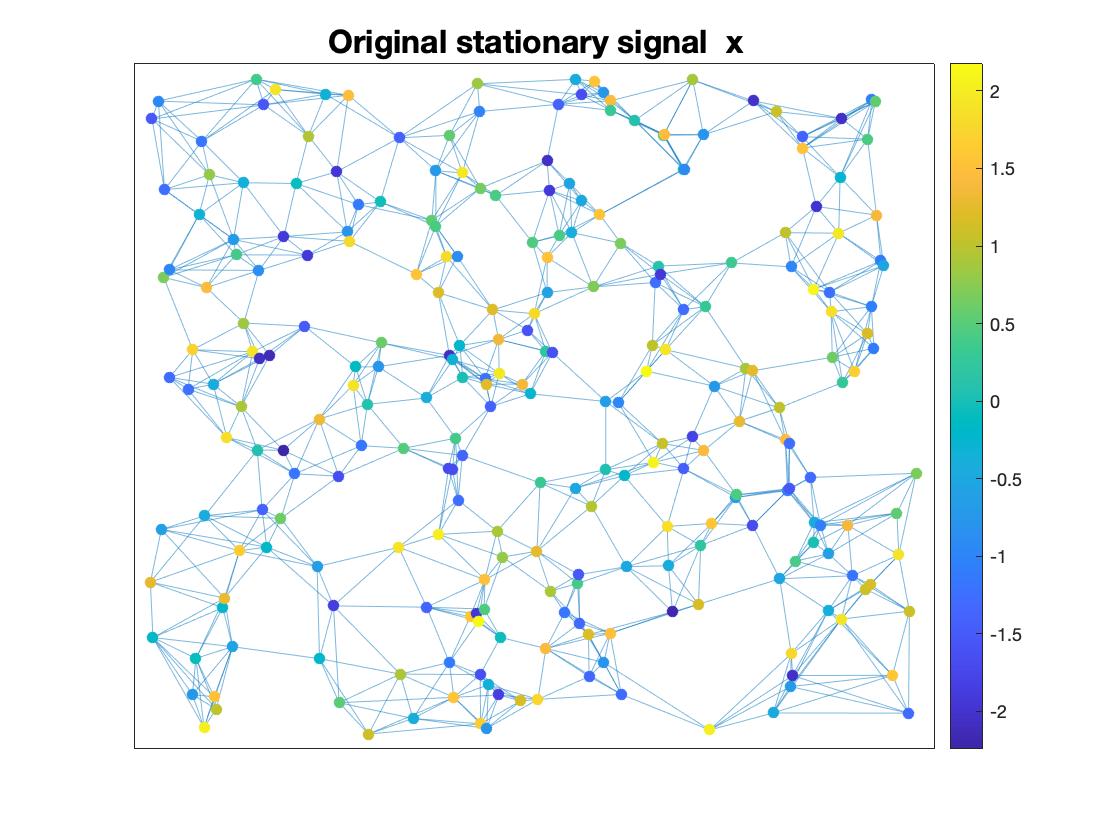
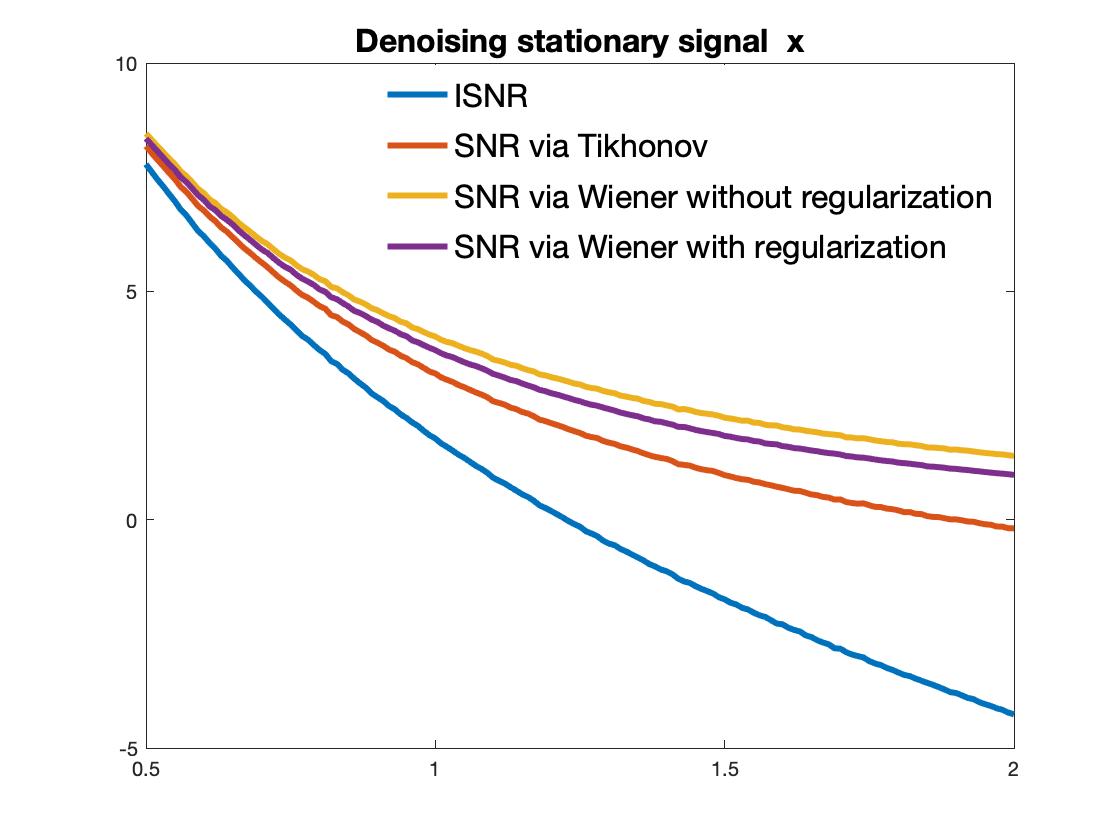
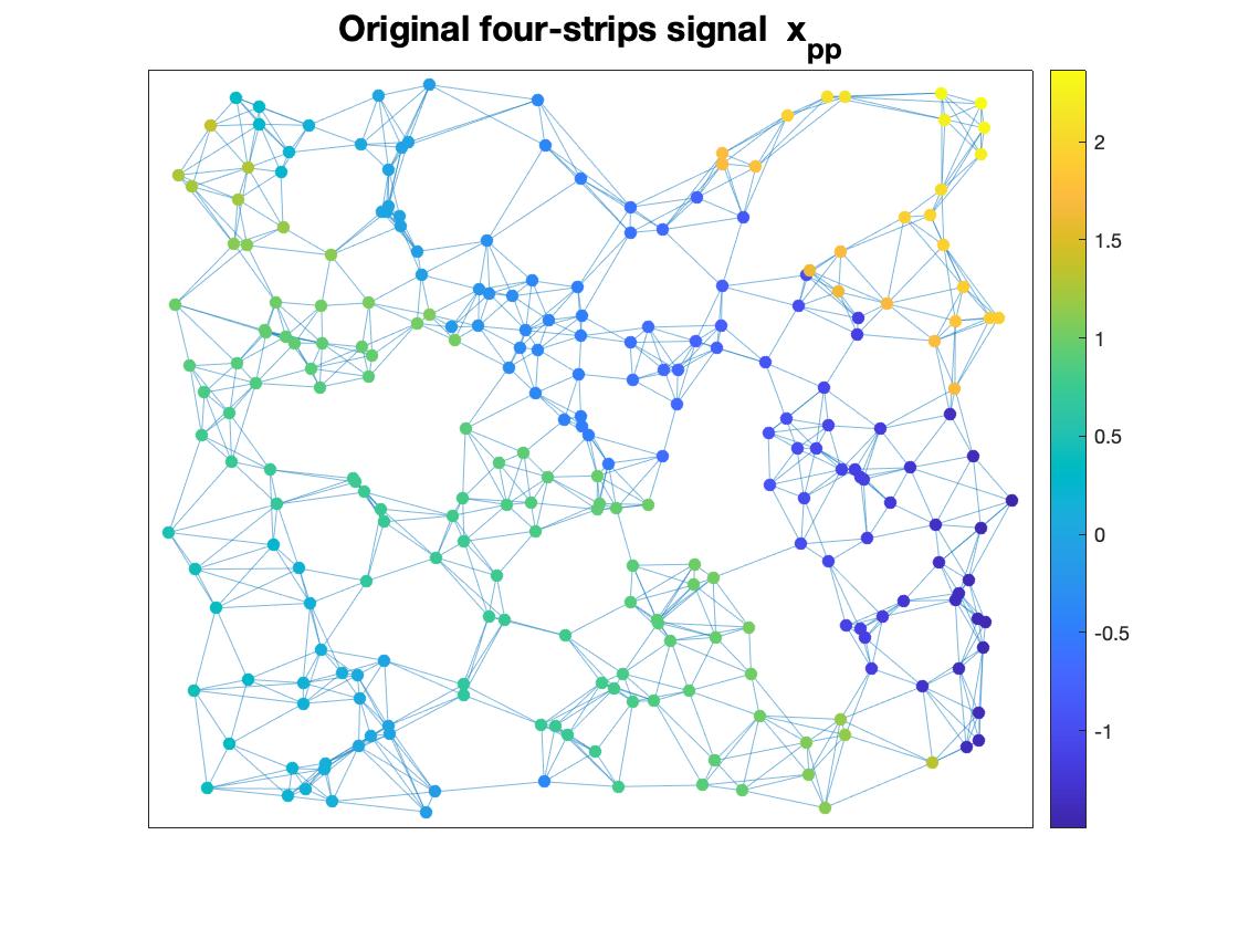
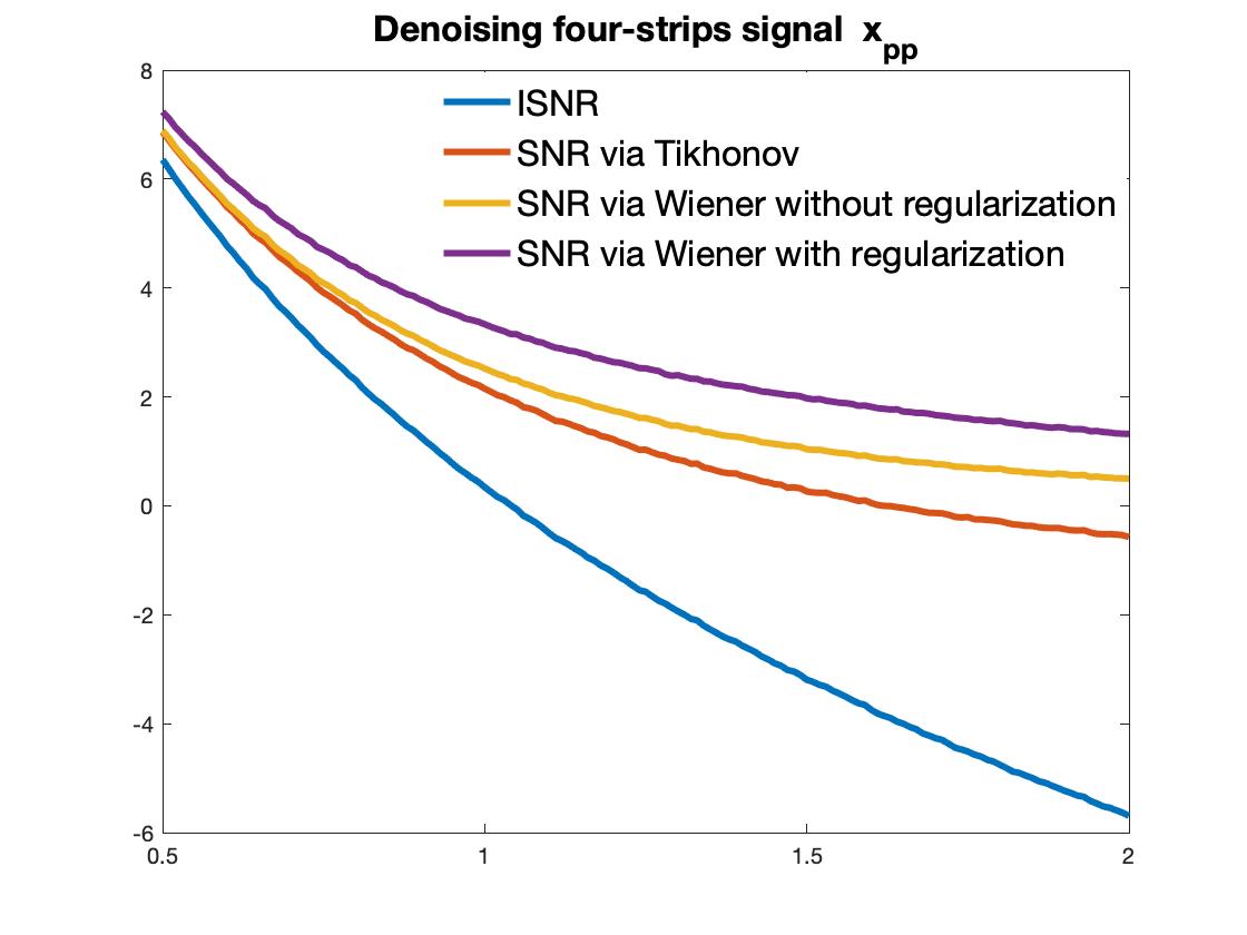
Figure 2: Plotted are the stationary signal ${\bf x}$ with correlation matrix ${\bf I}+{\bf L}^{\rm sym}/2$ (top left), the four-strip signal ${\bf x}_{\rm pp}$ in [18] (bottom left), and the averages of the input signal-to-noise ratio ${\rm ISNR}$ and output signal-to-noise ratio ${\rm SNR}$ of denoising stationary signals ${\bf x}$ (top right) and the four-strip signal ${\bf x}_{\rm pp}$ (bottom right) via the Wiener procedures without/with regularization and Tikhonov regularization approach over 1000 trials for different noise levels $0.5\leq\varepsilon\leq 2$.

Graph signals ${\bf x}$ in many applications exhibit some smoothness, which is widely measured by the ratio ${\bf x}^{T}{\bf L}^{\rm sym}{\bf x}/\|{\bf x}\|_{2}^{2}$. Observe that stationary signals ${\bf x}$ in the above simulations does not have good regularity as ${\mathbb{E}}{\bf x}^{T}{\bf L}^{\rm sym}{\bf x}/{\mathbb{E}}\|{\bf x}\|_{2}^{2}\in[1,4/3]$. We believe that it could be the reason that Wiener procedure with regularization has slightly poor performance on denoising than the Wiener procedure without regularization does.

Let ${\bf x}_{\rm pp}$ be the four-strip signal on the random geometric graph that impose the polynomial $0.5-2c_{x}$ on the first and third diagonal strips and $0.5+c_{x}^{2}+c_{y}^{2}$ on the second and fourth strips respectively, where $(c_{x},c_{y})$ are the coordinates of vertices [18, Fig. 2]. We do simulations on denoising the four-strip signal ${\bf x}_{\rm pp}$, i.e., we apply the same Tikhonov regularization and Wiener procedures with/without regularization except that stationary signals ${\bf x}$ is replaced by ${\bf x}_{\rm pp}$, see Figure 2. This indicates that Wiener procedure with regularization may have the best performance on denoising signals with certain regularity.

6-C Denoising wide-band stationary signals on random geometric graphs

In this subsection, we consider denoising wide-band stationary signals ${\bf x}$ in (4.2) on a random geometric graph ${\cal G}_{256}$ with

$${\mathbb{E}}{\bf x}=c{\bf 1}\ \ {\rm and}\ \ {\mathbb{E}}({\bf x}-{\mathbb{E}}{\bf x})({\bf x}-{\mathbb{E}}{\bf x})^{T}={\bf I}+{\bf L}^{\rm sym}/2,$$

where $c\neq 0$ is not necessarily to be given in advance. The observations ${\bf y}={\bf x}+\boldsymbol{\epsilon}$ are the inputs ${\bf x}$ corrupted by some additive noises $\boldsymbol{\epsilon}$ which is independent of the input signal ${\bf x}$ and whose covariance matrix is ${\bf G}=\varepsilon^{2}{\bf L}^{\rm sym}$ for some $\varepsilon>0$, and we select the uniform probability measure $\bf P$ in the stochastic mean squared error. In other words, we consider the Wiener filtering procedure (4.9) in the scenario that

$${\bf H}={\bf I},\widetilde{\bf R}={\bf I}+{\bf L}^{\rm sym}/2,{\bf P}=N^{-1}{\bf I}\ {\rm and}\ {\bf G}=\varepsilon^{2}{\bf L}^{\rm sym}.$$

Similar to the simulations in Section 6-B, we test the performance of the Wiener procedures with/without regularization and Tikhonov regularization on denoising wide-band stationary signals. From the simulation results presented in Figure 3, we see that the Wiener procedure with regularization has slightly poor performance on denoising than the Wiener procedure without regularization does, but they both perform better than Tikhonov regularization approach does.

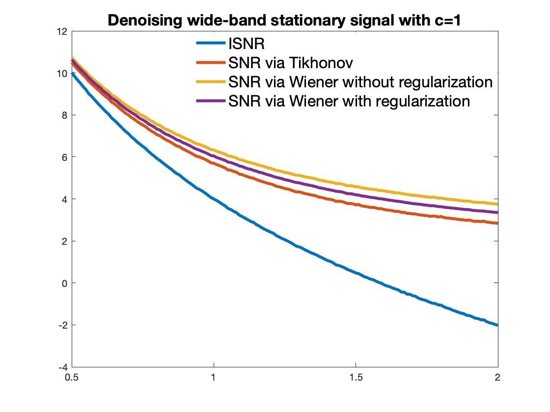
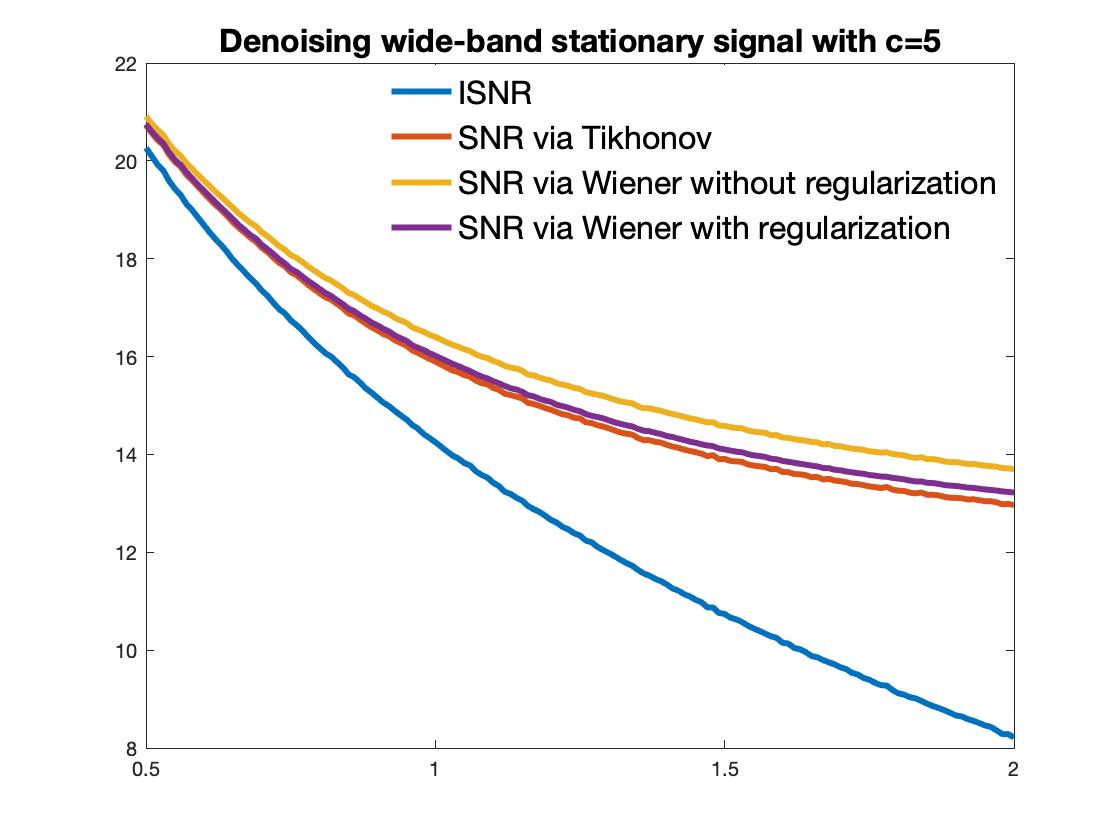
Figure 3: Plotted are the averages of the input signal-to-noise ratio ${\rm ISNR}$ and output signal-to-noise ratio ${\rm SNR}$ obtained by the Wiener procedures without/with regularization and Tikhonov regularization approach over 1000 trials for different noise levels $0.5\leq\varepsilon\leq 2$, in which the original signal is wide-band stationary with $c=1$ (left) and $c=5$ (right) on the random geometric graph ${\cal G}_{256}$.

Appendix A Proof of Theorem 4.1

By (4.1b), (4.1c) and (4.1d), we have

$${\mathbb{E}}{\bf y}{\bf y}^{T}={\bf H}{\bf R}{\bf H}^{T}+{\bf G}\ \ {\rm and}\ \ {\mathbb{E}}{\bf y}{\bf x}^{T}={\bf H}{\bf R}.$$ (A.1)

By (4.1b), (4.3) and (A.1), we obtain

$$\hskip-5.78172ptF_{{\rm mse},P,{\bf K}}({\bf W})$$ (A.2)

$$\hskip-5.78172pt= \hskip-5.78172pt{\rm tr}\left({\bf P}{\mathbb{E}}(({\bf W}{\bf y}-{\bf x})({\bf W}{\bf y}-{\bf x})^{T}\right)+{\rm tr}{\bf W}^{T}{\bf K}{\bf W}{\mathbb{E}}({\bf y}{\bf y}^{T})$$

$$\hskip-5.78172pt= \hskip-5.78172pt{\rm tr}\big{(}{\bf W}^{T}({\bf P}+{\bf K}){\bf W}({\bf H}{\bf R}{\bf H}^{T}+{\bf G})\big{)}+{\rm tr}({\bf P}{\bf R})$$

$$\hskip-5.78172pt-{\rm tr}({\bf H}{\bf R}{\bf P}{\bf W})-{\rm tr}({\bf W}^{T}{\bf P}{\bf R}{\bf H}^{T}).$$

Substituting ${\bf W}$ in (A.2) by ${\bf W}_{\rm mse}$ proves (4.6).

By (4.4) and (A.2), we obtain

$$F_{{\rm mse},P,{\bf K}}({\bf W})$$ (A.3)

$$\hskip-5.78172pt= \hskip-5.78172ptF_{{\rm mse},P,{\bf K}}({\bf W}_{\rm mse})+{\rm tr}\big{(}{\bf V}^{T}({\bf P}+{\bf K}){\bf V}({\bf H}{\bf R}{\bf H}^{T}+{\bf G})\big{)}$$

$$+{\rm tr}\big{(}{\bf V}^{T}({\bf P}+{\bf K}){\bf W}_{\rm mse}({\bf H}{\bf R}{\bf H}^{T}+{\bf G})-{\bf V}^{T}{\bf P}{\bf R}{\bf H}^{T}\big{)}$$

$$+{\rm tr}\big{(}{\bf W}_{\rm mse}^{T}({\bf P}+{\bf K}){\bf V}({\bf H}{\bf R}{\bf H}^{T}+{\bf G})-{\bf H}{\bf R}{\bf P}{\bf V}\big{)}$$

$$\hskip-5.78172pt= \hskip-5.78172ptF_{{\rm mse},P,{\bf K}}({\bf W}_{\rm mse})+{\rm tr}\big{(}({\bf H}{\bf R}{\bf H}^{T}+{\bf G})^{1/2}$$

$$\qquad\qquad\times{\bf V}^{T}({\bf P}+{\bf K}){\bf V}({\bf H}{\bf R}{\bf H}^{T}+{\bf G})^{1/2}\big{)}$$

$$\hskip-5.78172pt\geq \hskip-5.78172ptF_{{\rm mse},P,{\bf K}}({\bf W}_{\rm mse}),$$

where ${\bf V}={\bf W}-{\bf W}_{\rm mse}$, the first and second equality follows from (A.2) and (4.4) respectively, and the inequality holds as $({\bf H}{\bf R}{\bf H}^{T}+{\bf G})^{1/2}{\bf V}^{T}({\bf P}+{\bf K}){\bf V}({\bf H}{\bf R}{\bf H}^{T}+{\bf G})^{1/2}$ are positive semidefinite for all matrices ${\bf V}$. This proves that ${\bf W}_{\rm mse}$ is a minimizer to the minimization problem $\min_{\bf W}F_{{\rm mse},P,{\bf K}}({\bf W})$.

The conclusion that ${\bf W}_{\rm mse}$ is a unique minimizer to the minimization problem $\min_{\bf W}F_{{\rm mse},P,{\bf K}}({\bf W})$ follows from (A.3) and the assumptions that ${\bf P}+{\bf K}$ and ${\bf H}{\bf R}{\bf H}^{T}+{\bf G}$ are strictly positive definite.

Appendix B Proof of Theorem 5.1

Define the worst-case mean squared error of a reconstruction vector ${\bf w}$ with respect to a given unit vector ${\bf u}$ by

$$f_{{\rm wmse},{\bf u}}({\bf w})=\max_{\|{\bf x}\|_{2}\leq\delta_{0}}{\mathbb{E}}|{\bf w}^{T}{\bf y}-{\bf u}^{T}{\bf x}|^{2}$$ (B.1)

and set

$${\bf w}_{{\rm wmse},{\bf u}}={\bf W}_{{\rm wmse}}^{T}{\bf u}.$$ (B.2)

By direct computation, we have

$$F_{{\rm wmse},P}({\bf W})=\sum_{i\in V}p(i)f_{{\rm wmse},{\bf e}_{i}}({\bf W}^{T}{\bf e}_{i}),$$ (B.3)

where ${\bf e}_{i},i\in V$, are delta signals taking value one at vertex $i$ and zero at all other vertices. Then it suffices to show that ${\bf w}_{{\rm wmse},{\bf u}}$ is the optimal reconstructing vector with respect to the measurement $f_{{\rm wmse},{\bf u}}({\bf w})$, i.e.,

$${\bf w}_{{\rm wmse},{\bf u}}=\arg\min_{\bf w}f_{{\rm wmse},{\bf u}}({\bf w}).$$ (B.4)

By (5.2), (5.3) and the assumption $\|{\bf u}\|_{2}=1$, we have

$$\hskip-13.00806ptf_{{\rm wmse},{\bf u}}({\bf w}) \hskip-5.78172pt= \hskip-5.78172pt\max_{\|{\bf x}\|_{2}\leq\delta_{0}}{\mathbb{E}}|({\bf w}^{T}{\bf H}-{\bf u}^{T}){\bf x}+{\bf w}^{T}{\boldsymbol{\epsilon}}|^{2}$$

$$\hskip-5.78172pt= \hskip-5.78172pt\max_{\|{\bf x}\|_{2}\leq\delta_{0}}\big{|}({\bf w}^{T}{\bf H}-{\bf u}^{T}){\bf x}\big{|}^{2}+{\mathbb{E}}|{\bf w}^{T}{\boldsymbol{\epsilon}}|^{2}$$

$$\hskip-5.78172pt= \hskip-5.78172pt\delta_{0}^{2}({\bf w}^{T}{\bf H}-{\bf u}^{T})({\bf H}^{T}{\bf w}-{\bf u})+{\bf w}^{T}{\bf G}{\bf w}$$

$$\hskip-5.78172pt= \hskip-5.78172pt{\bf w}^{T}\big{(}\delta_{0}^{2}{\bf H}{\bf H}^{T}+{\bf G}){\bf w}-2\delta_{0}^{2}{\bf w}^{T}{\bf H}{\bf u}+\delta_{0}^{2}.$$

Therefore

$$\hskip-13.00806ptf_{{\rm wmse},{\bf u}}({\bf w}) \hskip-5.78172pt= \hskip-5.78172ptf_{{\rm wmse},{\bf u}}({\bf w}_{{\rm wmse},{\bf u}})+{\bf v}^{T}\big{(}\delta_{0}^{2}{\bf H}{\bf H}^{T}+{\bf G}){\bf v}$$ (B.5)

$$+2{\bf v}^{T}\Big{(}\big{(}\delta_{0}^{2}{\bf H}{\bf H}^{T}+{\bf G}\big{)}{\bf w}_{{\rm wmse},{\bf u}}-\delta_{0}^{2}{\bf H}{\bf u}\Big{)}$$

$$\hskip-5.78172pt= \hskip-5.78172ptf_{{\rm wmse},{\bf u}}({\bf w}_{{\rm wmse},{\bf u}})+{\bf v}^{T}\big{(}\delta_{0}^{2}{\bf H}{\bf H}^{T}+{\bf G}){\bf v}$$

$$\hskip-5.78172pt\geq \hskip-5.78172ptf_{{\rm wmse},{\bf u}}({\bf w}_{{\rm wmse},{\bf u}}),$$

where ${\bf v}={\bf w}-{\bf w}_{{\rm wmse},{\bf u}}$ and the last inequality holds as $\delta_{0}^{2}{\bf H}{\bf H}^{T}+{\bf G}$ is strictly positive definite. This proves (B.4) and hence that ${\bf W}_{\rm wmse}$ is a minimizer of the minimization problem (5.5), i.e., the inequality in (5.6) holds.

By (B.2), (B.3) and (B.4), we have

$$\hskip-5.78172ptF_{{\rm wmse},P}({\bf W}_{\rm wmse})=\sum_{i\in V}p(i)f_{i}({\bf w}_{{\rm wmse},{\bf e}_{i}})$$

$$\hskip-5.78172pt= \hskip-5.78172pt\sum_{i\in V}p(i)\big{(}-\delta_{0}^{4}{\bf e}_{i}^{T}{\bf H}^{T}(\delta_{0}^{2}{\bf H}{\bf H}^{T}+{\bf G})^{-1}{\bf H}{\bf e}_{i}+\delta_{0}^{2}\big{)}$$

$$\hskip-5.78172pt= \hskip-5.78172pt\delta_{0}^{2}-\delta_{0}^{4}{\rm tr}({\bf P}{\bf H}^{T}(\delta_{0}^{2}{\bf H}{\bf H}^{T}+{\bf G})^{-1}{\bf H}\big{)}$$

$$\hskip-5.78172pt= \hskip-5.78172pt\delta_{0}^{2}-\delta_{0}^{4}{\rm tr}((\delta_{0}^{2}{\bf H}{\bf H}^{T}+{\bf G})^{-1}{\bf H}{\bf P}{\bf H}^{T}\big{)}.$$

This proves the equality in (5.6) and hence completes the proof of the conclusion (5.6).

The uniqueness of the minimization problem (5.5) follows from (B.3) and (B.5), and the strictly positive definiteness of the matrices $\bf P$ and $\delta_{0}^{2}{\bf H}{\bf H}^{T}+{\bf G}$.

Acknowledgement  The authors would like to thank Professors Xin Li, Zuhair Nashed, Paul Nevai and Yuan Xu, and Dr. Nazar Emirov for their help during the preparation of this manuscript.

References

- [1] S. Wasserman and K. Faust, Social Network Analysis: Methods and Applications, Cambridge University Press, 1994.
- [2] C. Chong and S. Kumar, “Sensor networks: evolution, opportunities, and challenges,” Proc. IEEE, vol. 91, pp. 1247-1256, Aug. 2003.
- [3] G. Mao, B. Fidan, and B. D. O. Anderson, “Wireless sensor network localization techniques,” Comput. Netw., vol. 51, no. 10, pp. 2529-2553, July 2007.
- [4] J. Yick, B. Mukherjee, and D. Ghosal, “Wireless sensor network survey,” Comput. Netw., vol. 52, no. 12, pp. 2292-2330, Aug. 2008.
- [5] N. Motee and Q. Sun, “Sparsity and spatial localization measures for spatially distributed systems,” SIAM J. Control Optim., vol. 55, no. 1, pp. 200-235, Jan. 2017.
- [6] R. Hebner, “The power grid in 2030,” IEEE Spectrum, vol. 54, no. 4, pp. 50-55, Apr. 2017.
- [7] C. Cheng, Y. Jiang, and Q. Sun, “Spatially distributed sampling and reconstruction,” Appl. Comput. Harmon. Anal., vol. 47, no. 1, pp. 109-148, July 2019.
- [8] A. Sandryhaila and J. M. F. Moura, “Discrete signal processing on graphs,” IEEE Trans. Signal Process., vol. 61, no. 7, pp. 1644-1656, Apr. 2013.
- [9] D. I. Shuman, S. K. Narang, P. Frossard, A. Ortega, and P. Vandergheynst, “The emerging field of signal processing on graphs: Extending high-dimensional data analysis to networks and other irregular domains,” IEEE Signal Process. Mag., vol. 30, no. 3, pp. 83-98, May 2013.
- [10] A. Sandryhaila and J. M. F. Moura, “Discrete signal processing on graphs: Frequency analysis,” IEEE Trans. Signal Process., vol. 62, no. 12, pp. 3042-3054, June 2014.
- [11] M. M. Bronstein, J. Bruna, Y. LeCun, A. Szlam, and P. Vandergheynst, “Geometric deep learning: Going beyond Euclidean data,” IEEE Signal Process. Mag., vol. 34, no. 4, pp. 18-42, 2017.
- [12] A. Ortega, P. Frossard, J. Kovačević, J. M. F. Moura, and P. Vandergheynst, “Graph signal processing: Overview, challenges, and applications,” Proc. IEEE, vol. 106, no. 5, pp. 808-828, May 2018.
- [13] L. Stanković, M. Daković, and E. Sejdić, “Introduction to graph signal processing,” In Vertex-Frequency Analysis of Graph Signals, Springer, pp. 3-108, 2019.
- [14] X. Dong, D. Thanou, L. Toni, M. Bronstein, and P. Frossard, “Graph signal processing for machine learning: A review and new perspectives,” IEEE Signal Process. Mag., vol. 37, no. 6, pp. 117-127, 2020.
- [15] N. Emirov, C. Cheng, J. Jiang, and Q. Sun, “Polynomial graph filter of multiple shifts and distributed implementation of inverse filtering,” Sampl. Theory Signal Process. Data Anal., vol. 20, Article No. 2, 2022.
- [16] S. Segarra, A. G. Marques, and A. Ribeiro, “Optimal graph-filter design and applications to distributed linear network operators,” IEEE Trans. Signal Process., vol. 65, no. 15, pp. 4117-4131, Aug. 2017.
- [17] A. Gavili and X. Zhang, “On the shift operator, graph frequency, and optimal filtering in graph signal processing,” IEEE Trans. Signal Process., vol. 65, no. 23, pp. 6303-6318, Dec. 2017.
- [18] J. Jiang, C. Cheng, and Q. Sun, “Nonsubsampled graph filter banks: Theory and distributed algorithms,” IEEE Trans. Signal Process., vol. 67, no. 15, pp. 3938-3953, Aug. 2019.
- [19] R. A. Horn and C. R. Johnson. Matrix Analysis, Cambridge University Press, 2012.
- [20] E. Isufi, A. Loukas, A. Simonetto, and G. Leus, “Autoregressive moving average graph filtering,” IEEE Trans. Signal Process., vol. 65, no. 2, pp. 274-288, Jan. 2017.
- [21] W. Waheed and D. B. H. Tay, “Graph polynomial filter for signal denoising,” IET Signal Process., vol. 12, no. 3, pp. 301-309, Apr. 2018.
- [22] K. Lu, A. Ortega, D. Mukherjee, and Y. Chen, “Efficient rate-distortion approximation and transform type selection using Laplacian operators,” in 2018 Picture Coding Symposium (PCS), San Francisco, CA, June 2018, pp. 76-80.
- [23] D. I. Shuman, P. Vandergheynst, D. Kressner, and P. Frossard, “Distributed signal processing via Chebyshev polynomial approximation,” IEEE Trans. Signal Inf. Process. Netw., vol. 4, no. 4, pp. 736-751, Dec. 2018.
- [24] M. Coutino, E. Isufi, and G. Leus, “Advances in distributed graph filtering,” IEEE Trans. Signal Process., vol. 67, no. 9, pp. 2320-2333, May 2019.
- [25] C. Cheng, J. Jiang, N. Emirov, and Q. Sun, “Iterative Chebyshev polynomial algorithm for signal denoising on graphs,” in Proceeding 13th Int. Conf. on SampTA, Bordeaux, France, Jul. 2019, pp. 1-5.
- [26] J. Jiang, D. B. Tay, Q. Sun, and S. Ouyang, “Design of nonsubsampled graph filter banks via lifting schemes,” IEEE Signal Process. Lett., vol. 27, pp. 441-445, Feb. 2020.
- [27] S. Chen, A. Sandryhaila, and J. Kovačević, “Distributed algorithm for graph signal inpainting,” in 2015 IEEE International Conference on Acoustics, Speech and Signal Processing (ICASSP), Brisbane, QLD, Apr. 2015, pp. 3731-3735.
- [28] X. Shi, H. Feng, M. Zhai, T. Yang, and B. Hu, “Infinite impulse response graph filters in wireless sensor networks,” IEEE Signal Process. Lett., vol. 22, no. 8, pp. 1113-1117, Aug. 2015.
- [29] S. Chen, A. Sandryhaila, J. M. F. Moura, and J. Kovačević, “Signal recovery on graphs: variation minimization,” IEEE Trans. Signal Process., vol. 63, no. 17, pp. 4609-4624, Sept. 2015.
- [30] M. Onuki, S. Ono, M. Yamagishi, and Y. Tanaka, “Graph signal denoising via trilateral filter on graph spectral domain,” IEEE Trans. Signal Inf. Process. Netw., vol. 2, no. 2, pp. 137-148, June 2016.
- [31] C. Cheng, N. Emirov, and Q. Sun, “Preconditioned gradient descent algorithm for inverse filtering on spatially distributed networks,” IEEE Signal Process. Lett., vol. 27, pp. 1834-1838, Oct. 2020.
- [32] N. Bi, M. Z. Nashed, and Q. Sun, “Reconstructing signals with finite rate of innovation from noisy samples,” Acta Appl. Math., vol. 107, no. 1, pp. 339-372, July 2009.
- [33] B. Girault, “Stationary graph signals using an isometric graph translation,” in Proc. 23rd Eur. Signal Process. Conf., 2015, pp. 1516-1520.
- [34] N. Perraudin and P. Vandergheynst, “Stationary signal processing on graphs”, IEEE. Trans. Signal Process., vol. 65, no. 13, pp. 3462-3477, July 2017.
- [35] S. Segarrat, A. G. Marques, G. Leus, and A. Ribeiro, “Stationary graph processes: parametric power spectal estimation,” in 2017 IEEE International Conference on Acoustics, Speech and Signal Processing (ICASSP), New Orleans, LA, USA, pp. 4099-4103, Mar. 2017.
- [36] A. C. Yagan and M. T. Ozgen, “Spectral graph based vertex-frequency Wiener filtering for image and graph signal denoising,” IEEE Trans. Signal Inf. Process., vol. 6, pp. 226-240, Feb. 2020.
- [37] D. I. Shuman, P. Vandergheynst, D. Kressner, and P. Frossard, “Distributed signal processing via Chebyshev polynomial approximation,” IEEE Trans. Signal Inf. Process. Netw., vol. 4, no. 4, pp. 736-751, Dec. 2018.
- [38] E. Isufi, A. Loukas, N. Perraudin, and G. Leus, “Forecasting time series with VARMA recursions on graphs,” IEEE Trans. Signal Process., vol. 67, no. 18, pp. 4870-4885, Sept. 2019.
- [39] M. E. H. Ismail, Classical and Quantum Orthogonal Polynomials in One Variable, Cambridge University Press, Aug. 2009.
- [40] J. Shen, T. Tang, and L.-L. Wang, Spectral Methods: Algorithms, Analysis and Applications, Springer, Aug. 2011.
- [41] L. N. Trefethen, Approximation Theory and Approximation Practice, Society for Industrial and Applied Mathematics (SIAM), Philadelphia, PA, 2013.
- [42] H. Wang and S. Xiang, “On the convergence rates of Legendre approximation,” Math. Comput., vol. 81, no. 278, pp. 861-877, Apr. 2011
- [43] S. Wang, “On Error bounds for orthogonal polynomial expansions and Gauss-type quadrature,” SIAM J. Numer. Anal., vol. 50, no. 3, pp. 1240-1263, 2012.
- [44] Y. Eldar and M. Unser, “Nonideal sampling and interpolation from noisy observations in shift-invariant spaces,” IEEE Trans. Signal Process., vol. 54, no. 7, pp. 2636-2651, June 2006.
- [45] V. N. Ekambaram, G. C. Fanti, B. Ayazifar, and K. Ramchandran, “Circulant structures and graph signal processing,” in Proc. IEEE Int. Conf. Image Process., 2013, pp. 834-838.
- [46] V. N. Ekambaram, G. C. Fanti, B. Ayazifar, and K. Ramchandran, “Multiresolution graph signal processing via circulant structures,” in Proc. IEEE Digital Signal Process./Signal Process. Educ. Meeting (DSP/SPE), 2013, pp. 112-117.
- [47] M. S. Kotzagiannidis and P. L. Dragotti, “Splines and wavelets on circulant graphs,” Appl. Comput. Harmon. Anal., vol. 47, no. 2, pp. 481-515, Sept. 2019.
- [48] M. S. Kotzagiannidis and P. L. Dragotti, “Sampling and reconstruction of sparse signals on circulant graphs – an introduction to graph-FRI,” Appl. Comput. Harmon. Anal., vol. 47, no. 3, pp. 539-565, Nov. 2019.
- [49] P. Nathanael, J. Paratte, D. Shuman, L. Martin, V. Kalofolias, P. Vandergheynst, and D. K. Hammond, “GSPBOX: A toolbox for signal processing on graphs,” arXiv:1408.5781, Aug. 2014.