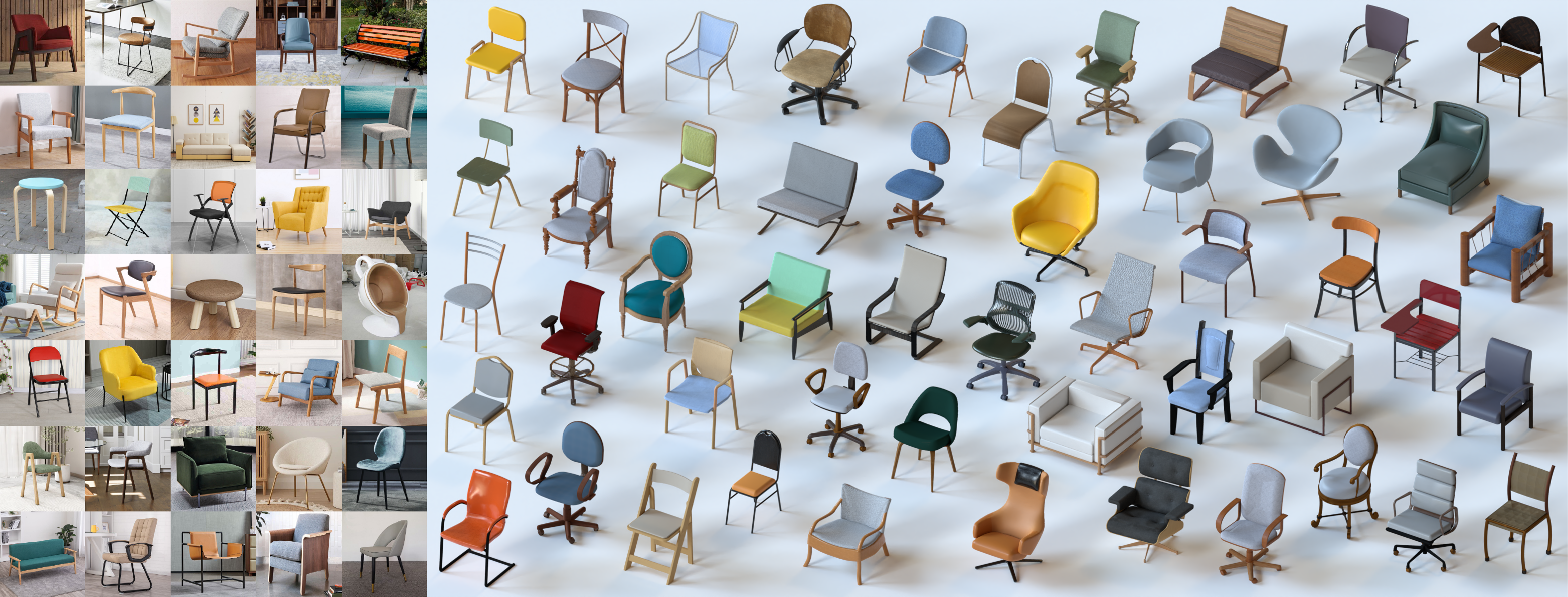
Figure 1. A sample of PhotoShapes (shapes with realistic relightable materials) created with our material assignment method by transferring materials from photo exemplars to 3D shapes with diverse structures, where the input exemplars are the photos in-the-wild on the left.

Photo-to-Shape Material Transfer for Diverse Structures

Abstract.

We introduce a method for assigning photorealistic relightable materials to 3D shapes in an automatic manner. Our method takes as input a photo exemplar of a real object and a 3D object with segmentation, and uses the exemplar to guide the assignment of materials to the parts of the shape, so that the appearance of the resulting shape is as similar as possible to the exemplar. To accomplish this goal, our method combines an image translation neural network with a material assignment neural network. The image translation network translates the color from the exemplar to a projection of the 3D shape and the part segmentation from the projection to the exemplar. Then, the material prediction network assigns materials from a collection of realistic materials to the projected parts, based on the translated images and perceptual similarity of the materials.

One key idea of our method is to use the translation network to establish a correspondence between the exemplar and shape projection, which allows us to transfer materials between objects with diverse structures. Another key idea of our method is to use the two pairs of (color, segmentation) images provided by the image translation to guide the material assignment, which enables us to ensure the consistency in the assignment. We demonstrate that our method allows us to assign materials to shapes so that their appearances better resemble the input exemplars, improving the quality of the results over the state-of-the-art method, and allowing us to automatically create thousands of shapes with high-quality photorealistic materials. Code and data for this paper are available at https://github.com/XiangyuSu611/TMT.

1. Introduction

Most applications of computer graphics require 3D shapes with materials, since the geometry of 3D shapes alone does not fully convey the appearance of an object to a human. Shapes with materials are important for rendering realistic 3D scenes, which are relevant in simulations, games, and AR/MR/VR. Materials can include colors and textures, but high-quality realistic materials that can be relit are usually represented as reflectance functions such as BRDFs or SVBRDFs. Moreover, manually assigning realistic materials to 3D meshes can be quite difficult, since the task involves experimentally selecting material parameters for patches of a 3D model according to a desired design, possibly also requiring the definition of texture coordinates. Thus, more automated ways of assigning materials to 3D shapes are necessary for mass content creation and customization.

One option to circumvent the problem of material assignment to shapes altogether is the reuse of existing shapes. However, the shapes in many datasets such as ShapeNet and PartNet only contain basic textures but no realistic materials. In addition, shape repositories are not guaranteed to contain the shapes that the user requires; the user may need to apply materials to a specific 3D model. On the other hand, recently there have been great advances in shape reconstruction with the use of deep learning. Methods have been introduced to reconstruct shapes from different input types such as point clouds (Park et al., 2019; Chibane et al., 2020), photographs (Ji et al., 2017; Han et al., 2021), and sketches (Wu et al., 2017; Delanoy et al., 2018). Thus, this is a promising direction for the automated creation of shapes. However, in the majority of these methods, materials are not accounted for in the learning and reconstruction, and thus the generated shapes possess only their geometry.

In this paper, we introduce a method for automatically assigning realistic materials to 3D shapes to alleviate this gap in the automated creation of 3D shapes. Our setting is similar to that of previous work (Park et al., 2018), where our method uses photos of real objects as exemplars that guide the assignment of materials to 3D shapes, generating collections of PhotoShapes (Figure 1). Note that, PhotoShapes, as defined by Park et al. (2018), are not simply textured shapes, but shapes with realistic materials that can be relit, given that they are represented as reflectance functions possibly with additional texture information. As a consequence, the creation of PhotoShapes is also a different problem than simply transferring the texture of a reference photo to a 3D shape  (Wang et al., 2016).

The creation of PhotoShapes has several challenges of its own. First, in texture transfer, the texture of the input exemplar can be directly transferred to the 3D model after the removal of illumination shading and projection distortions. On the other hand, the assignment of realistic materials requires a mapping from the material in the photograph to a database of reflectance functions, since the photograph itself does not contain such information. The material database needs to be sufficiently diverse. Moreover, the extraction of material information from the exemplar and transfer to the 3D model requires a mapping from the geometry and structure of the object in the 2D exemplar to the geometry and structure of the 3D shape, which can be a difficult matching problem.

Previous work has studied these problems and introduced methods for shape material assignment and shape reconstruction with materials. As representative examples of recent work in this area, Wang et al.  (2016) transfer the texture from an exemplar image to a collection of shapes with an alignment method. The notable work of Park et al. (2018) uses collections of shapes, materials, and photos to create thousands of PhotoShapes, where their method uses a CNN to predict material properties for shape segments. Oechsle et al. (2019) learn a spatial function that represents texture information and can be used to assign textures to 3D models. However, most of these methods either do not assign realistic materials or assume that a good alignment exists between the object in the exemplar and the 3D shape, and thus use local correspondence approaches to compute the part mapping. Specifically, Park et al. (2018) rely heavily on a reliable matching between photos and shapes, which is usually hard to obtain by searching example photos for a given 3D shape.

In our paper, given a 3D shape with part segmentation and a photo exemplar of a shape from the same object category, we address these limitations so that the shape and object in the photo can have very different geometric structure. One key idea of our method is that we use a state-of-the-art image translation network to establish a mapping between the parts of the two objects, which provides a more robust correspondence between the objects for material transfer. Specifically, the translation network transfers the color from the exemplar to a projection of the 3D shape, and the part segmentation from the projection to the exemplar (Figure 2). The correspondence is then used by a material assignment network to assign materials to the parts of the 3D object, so that the materials are similar to those in the corresponding parts of the exemplar. Another innovation over previous work is that our material assignment network accomplishes this step by considering the perceptual similarity of the materials. In addition, since the image translation results in two (color, segmentation) pairs, we use the two image pairs to further ensure the consistency of the material assignment.

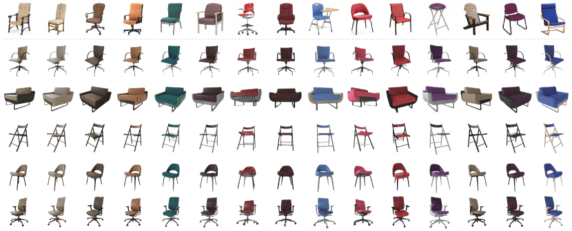
Figure 6. Results of our method for transferring materials from exemplars to 3D shapes. We show results generated from different combinations of photo exemplars (given in the top row) and shapes (given in the remaining rows). Note the realism of the assigned materials, the resemblance of the results to the exemplars, and the diversity of structures in the shapes and exemplars.

Given these contributions, we are able to create a variety of PhotoShapes (Figure 6). The generated PhotoShapes have materials closer in appearance to the exemplars when compared to the results of previous work. We demonstrate this improvement with visual and quantitative evaluations of our method, involving a comparison to baselines and the state-of-the-art method. We also show the effect of the different components of our method in the results.

In summary, our contributions include the introduction of:

• An image translation network for establishing correspondences between diverse structures in shapes and photographs, and transferring color and segmentation information;

• A material prediction network that assigns photorealistic materials to shape parts based on the result of image translation and a learned feature space of material perceptual similarity;

• A material transfer method combining the image translation and material prediction networks with a material assignment consistency criterion.

2. Related Work

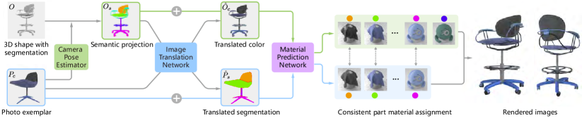
Figure 2. Overview of our method for assigning photorealistic relightable materials to 3D shapes based on photo exemplars. Given a 3D shape with segmentation and photo exemplar as input, we first project the 3D shape from a similar view as the exemplar. Next, an image translation network translates the color from the exemplar to the projection and the part segmentation from the projection to the exemplar. Then, a material prediction network assigns materials to the projected parts based on the translated images. Note that the joint translation of segmentation and color enables us to better ensure the consistency in the material assignment step. The result of the method is a 3D shape that can be rendered from different viewpoints with realistic materials.

Appearance modeling, especially material capture and representation (Guarnera et al., 2016), has received much attention in computer graphics and vision. Related problems include the development of models for establishing material similarity (Lagunas et al., 2019a) or for editing materials (Serrano et al., 2016; Schmidt et al., 2016), and the introduction of large datasets of materials extracted from photographs (Bell et al., 2013, 2015). Since our goal is to produce realistic textured materials for 3D shapes, we focus our discussion of previous work on methods related to appearance transfer onto 3D shapes. We also discuss research on image translation which is related to our solution approach.

Appearance transfer onto 3D shapes. The line of research most related to our work aims to transfer a combination of color, material properties, or textures from a source such as a material database, a single image, or a collection of images, to target 3D models. Jain et al. (2012) introduced a method to automatically assign materials to 3D objects based on correlations learned from a dataset of 3D shapes with materials. Although the user can select different material suggestions provided by the system, the user cannot directly specify the desired materials, e.g., with an exemplar. Nguyen et al. (2012) introduced the first method to transfer material from an image or video to 3D geometry. However, the method focuses on transfer to 3D scenes composed of multiple objects, and uses a global optimization without 2D-3D alignment.

Moreover, Wang et al. (2016) transfer the texture from an exemplar input image to a collection of 3D shapes. The method rectifies the texture in the input image and then transfers the texture to a 3D shape that is geometrically similar to the object in the input image, further applying the texture to other models in the collection. Rematas et al. (2016) align a target 3D shape to a reference 2D photo and extract per-segment materials. Liu et al. (2017) color a 3D model based on an example photograph by establishing point correspondences between the image and 3D model, which are then used to transfer color information from the image to the model. Moreover, Zhu et al. (2018) colorize 3D furniture models and indoor scenes according to an image exemplar, based on transferring color information across image segmentations. Huang et al. (2018b) facilitate the transfer of a detailed texture from a photograph to a 3D model by aligning a simple proxy to the object in the photograph, which allows the method to extract the geometric detail of the object and a reflectance texture from the photograph. The extracted information can then be applied to new models.

With the advent of deep learning, Park et al. (2018) use shape collections, material collections, and photo collections to assign materials to 3D shapes with a CNN that predicts material properties for shape segments. Differently from most related work, their method assigns materials represented as SVBRDFs, producing photorealistic relightable 3D shapes (PhotoShapes), rather than models with only color or texture information. Raj et al. (2019) also use collections of 3D models and images to generate textured models. However, they perform the transfer in the image domain by rendering a model from a set of viewpoints and assigning textures to the resulting images, which are then fused together into a textured 3D model. Mir et al. (2020) specialize this type of method to transfer textures from images of clothing to 3D garment models.

Since we need to establish a correspondence between the exemplar image and 3D shape before appearance transfer, the material transfer pipeline can be naturally decomposed into two subtasks: 2D-3D alignment and information transfer. Thus, methods that address the general problem of 2D-3D alignment are also relevant to our work. Specifically, Rematas et al. (2016) align renderings of segmented shapes to images through a coarse-to-fine refinement method. Su et al. (2014) introduce a method that extracts silhouettes from renderings and an input image to establish a 2D-3D correspondence. Huang et al. (2015) use a method based on matching of patches to establish a 2D-3D correspondence.

Departing from the idea of an information transfer pipeline as introduced by the works discussed above, Oechsle et al. (2019) propose to represent texture information as a function in 3D space, similar to an implicit occupancy or signed distance function for representing a 3D shape (Park et al., 2019; Chen and Zhang, 2019). The function, coined a “texture field”, is learned with a set of neural networks, where the generation of the texture color for a 3D point is conditioned on an image and a shape. On the other hand, Hu et al. (2021) reconstruct a textured 3D point cloud from an input image, since points clouds are a more lightweight representation than volumes, meshes, or implicit functions. However, the resulting model and texture produced by the method are fixed by the input.

Discussion. The work of Park et al. (2018) is the most related to our work. Similarly to their work, our goal is to produce realistic PhotoShapes. However, differently from their solution, our method does not require an existing match between photos and shapes in the database. Instead, our method is able to transfer information from a photo exemplar with a significantly different geometric structure from the given 3D shape by relying on a matching of part segments obtained by image translation. This is more robust than the local alignment method of Park et al. (2018) that requires matching points to be sufficiently close, as it applies a projection followed by SIFT flow. Moreover, as discussed above, other works assign mainly colors or texture information to the 3D models rather than a complete material specification, and also have similar assumptions of geometric similarity of the photo’s object to the input 3D model or proxy shape. Furthermore, the texture field method, although interesting as an alternative to direct material transfer, requires the input model to be retrained for each input exemplar and does not assign 2D texture coordinates to the input 3D shape, resulting in textures that have mainly uniform colors.

Image translation. Exemplar-based image translation can be characterized as a form of conditional image synthesis where an input structure (segmentation mask, edge map, or set of pose keypoints) is converted into an image with the style of an input exemplar (Isola et al., 2017; Chen and Koltun, 2017; Huang et al., 2018a). This form of image translation requires to map the input structure to the exemplar image, establishing a cross-domain correspondence. In our work, we use image translation to map the texture of an input exemplar into the segmentation of a rendered image, and vice-versa, which serves as the first step of our material assignment pipeline. Specifically, we use the method of Zhang et al. (2020), where image translation and cross-domain correspondence are learned together with two jointly-trained neural networks, so that the solution of each task facilitates the other.

3. Overview

Figure 2 shows an overview of our method. The input to our method is a 3D shape with part segmentation and a photo exemplar of an object from the same category, which may have a totally different geometric structure than the given shape. We assume that the 3D shape is given with the part segmentation. However, note that such segmentation can be obtained automatically with existing methods (Kalogerakis et al., 2017; Mo et al., 2019; Pham et al., 2019). Our method starts by estimating the camera pose of the photo exemplar. Then, we project the 3D shape based on the camera pose and transfer the part segmentation from the 3D shape to the 2D projection, resulting in a labeled image that we call a semantic projection.

Next, our image translation network takes the photo exemplar and the semantic projection as input, and outputs two translated images. One image translates the color from the exemplar to the projection, and the other image translates the part segmentation from the projection to the exemplar. Note that we use the term translation in a similar manner as the related literature (Zhang et al., 2020), i.e., a transfer of color or structure information from one image to another, not to be confused with the spatial transformation. As a result, we get two (color, segmentation) image pairs. For each pair, we use our material prediction network to obtain a material assignment to the object parts, while at the same time we use the two image pairs to further ensure the consistency in the material assignment. Note that the use of two pairs of images is a key component of our method to ensure the assignment consistency and thus improve the quality of the result. The final part material assignment can then be used to render realistic images of the 3D shape with similar material as the photo exemplar.

Datasets.

Since our method is based on learning, we use collections of shapes, photographs, and materials for training our neural networks and evaluating our results. Note that shape and photograph collections are category-specific, while we use the same material collection for the different object categories tested. We extend the material collection provided by Park et al. (2018) by adding new, more distinctive materials, which results in a set of 600 materials in total. We group the materials into five categories: leathers, fabrics, woods, metals, and plastics. Since the collections do not directly provide samples of translated images and shapes, we use the collections to create synthetic data for training our networks, as in the work of Park et al. (2018). We describe more details about the collections and data generation in the supplementary material.

4. Material transfer method

In this section, we first explain the details of the two key components of our method: the networks for image translation and material prediction. Then, we explain how we combine the two networks together to perform the material transfer.

4.1. Image translation

Given the image exemplar, we first estimate the camera pose of the image and use it to generate the semantic projection (2D projection with part segmentation) of the given 3D shape. To obtain the camera pose, we adopt the camera pose estimation network proposed by Xu et al. (2019). Then, we project the 3D shape based on the camera pose and transfer the part segmentation from the 3D shape to the 2D projection to create the semantic projection.

Moreover, given the photo exemplar and the semantic projection, the goal of image translation is to generate both the part segmentation for the photo exemplar and the colored image for the semantic projection so that the colored image and semantic projection are in correspondence with each other. The two pairs of images are then used for part material prediction in the next step. However, the key challenge here is that such images with translated color do not naturally exist in the wild and thus we need to learn to establish a cross-domain correspondence between the exemplar and projection. To tackle this problem, we use the method of Zhang et al. (2020), where image translation and cross-domain correspondence are learned together with two jointly-trained neural networks.

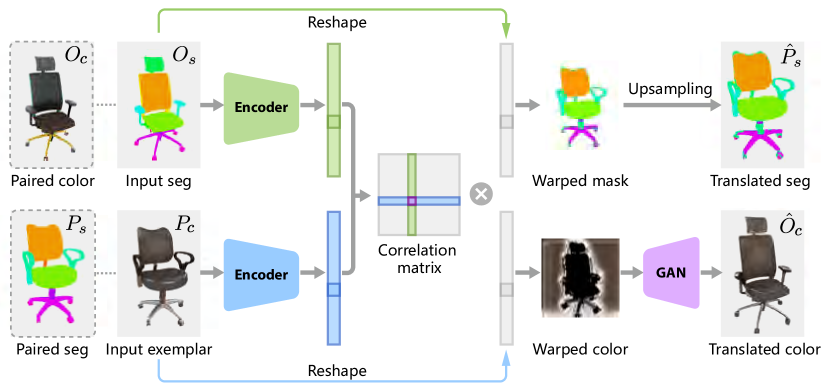
Figure 3. Image translation method used in our work, where the core components are based on the method of Zhang et al. (2020). Given the input semantic projection $O_{s}$ of a 3D object and the photo exemplar $P_{c}$, we establish a correspondence between the images, which is then used for image warping and information transfer, resulting in translated segmentation $\hat{P}_{s}$ and translated color $\hat{O}_{c}$ . Note that the paired color $O_{c}$ and segmentation mask $P_{s}$ are only used for training. Please refer to the text in Section 4.1 for more details.

Figure 3 shows a simplified diagram of the image translation method (Zhang et al., 2020). Given the semantic projection of the input object $O_{s}$ and the photo exemplar with color $P_{c}$, a first network embeds the two images into a common domain where it is possible to build a dense correspondence with a correspondence layer (Zhang et al., 2019). The correspondence is represented by a correlation matrix. Then, the input images are warped according to the correspondence, resulting in the translation of segmentation and color. After that, we upsample the translated segmentation to the same resolution as the input exemplar to obtain the translated segmentation $\hat{P}_{s}$, and apply an image synthesis GAN to the translated color to ensure that the generated image $\hat{O}_{c}$ looks more natural. Note that, in our notation, $s$ and $c$ refer to the two different translation domains (segmentation vs. color), and $O$ and $P$ refer to the different image contents (projection of 3D object vs. photo exemplar).

The main challenge of this cross-domain image translation problem is to learn the correspondence without direct supervision, since we do not have a ground truth $\hat{O}_{c}$ for the final output. Creating such ground truth is a difficult problem. Therefore, we instead make use of images that are easier to create, including the colored image $O_{c}$ corresponding to the input semantic projection $O_{s}$ and the segmentation image $P_{s}$ corresponding to the input colored exemplar $P_{c}$. This data is illustrated in the dashed boxes on the left of Figure 3. Thus, during the training of the translation method, quadruples $({\color[rgb]{0,0,0}\textbf{}O_{c}},O_{s},{\color[rgb]{0,0,0}\textbf{}P_{c}},P_{s})$ composed of two (color, segmentation) pairs are used to guide the training.

The loss function that guides the training the image translation network is defined as:

(1) $$L_{t}={\color[rgb]{0,0,0}\textbf{}L_{\text{col}}}+L_{\text{seg}}+L_{\text{reg}},$$

where $L_{\text{col}}$ is the color loss, $L_{\text{seg}}$ is the segmentation loss, and $L_{\text{reg}}$ is the regularization loss. The first two terms ensure that the translated color and segmentation are similar to the corresponding ground truth data and look natural, while the last term regularizes the correspondence between the input pairs from two different domains.

4.1.1. Color loss.

The loss $L_{\text{col}}$ is mainly used to constrain the translated color $\hat{O}_{c}$, and is defined as:

(2) $$L_{\text{col}}=\psi_{1}{\color[rgb]{0,0,0}\textbf{}L_{\text{context}}^{\text{col}}}+\psi_{2}L_{\text{perc}}+\psi_{3}L_{\text{feat}}+\psi_{4}L_{\text{adv}},$$

where 1) $L_{\text{context}}^{\text{col}}$ is the context loss to minimize the low-level feature distance between $\hat{O}_{c}$ and $P_{c}$ for any given exemplar $P_{c}$ as the color is translated from $P_{c}$; 2) $L_{\text{perc}}$ is the perceptual loss to minimize the high-level feature distance between $\hat{O}_{c}$ and $O_{c}$ for any given exemplar $P_{c}$, as it shares the same structure with $O_{c}$; 3) $L_{\text{feat}}$ is the feature matching loss to minimize the feature distance between $\hat{O}_{c}$ and $O_{c}$ when the input is a pseudo-exemplar pair $(O_{s},{\color[rgb]{0,0,0}\textbf{}{O}^{{}^{\prime}}_{c}})$, with ${O}^{{}^{\prime}}_{c}$ obtained by applying random geometric distortion to $O_{c}$, as the color is kept the same during the distortion; 4) $L_{\text{adv}}$ is the adversarial loss to ensure that the synthesized images $\hat{O}_{c}$ look indistinguishable from real ones.

4.1.2. Segmentation loss

The loss $L_{\text{seg}}$ is mainly used to constrain the translated segmentation $\hat{P}_{s}$, and is defined as:

(3) $$L_{\text{seg}}=\psi_{5}L_{\text{pred}}+\psi_{6}L_{\text{context}}^{\text{seg}},$$

where $L_{\text{pred}}$ is the prediction loss to minimize the distance between $\hat{P}_{s}$ and $P_{s}$ for any given semantic segmentation mask $O_{s}$, and $L_{\text{context}}^{\text{seg}}$ is the perceptual loss to minimize the low-level feature distance between $\hat{P}_{s}$ and $P_{s}$ for a given semantic segmentation mask $O_{s}$.

4.1.3. Regularization loss

The loss $L_{\text{reg}}$ is used to regularize the embedding in the shared domain of both inputs, and is defined as:

(4) $$L_{\text{reg}}=\psi_{7}L_{\text{align}}+\psi_{8}L_{\text{cycle}},$$

where $L_{\text{align}}$ is the domain alignment loss to minimize the feature distance between $O_{s}$ and $O_{c}$ after embedding in the shared feature space, and $L_{\text{cycle}}$ is the correspondence regularization to ensure that the final output after a cycle process is similar to the input exemplar $P_{c}$.

For more details about the network architecture and loss definition, please refer to the supplementary material.

4.2. Material prediction

Given a pair composed of a colored image and its corresponding part segmentation image, the goal of the material prediction network is to obtain an optimal part material assignment for the input, similar to the method of Park et al. (2018). However, differently from their method, which treats the material prediction problem purely as a classification problem, we take the perceptual similarity between materials into consideration to assign materials that maximize the visual similarity between the material predicted for each segment and its corresponding patch in the colored image. The motivation for using the perceptual similarity is that then the network can perform a suitable material assignment even if the material label is incorrect. Thus, this step requires to learn the perceptual similarity between predicted materials and patches in the colored image.

To learn the perceptual similarity, we first prepare material images that will be used in the learning. We render an image for each material in our dataset with the specific scene and perspective settings proposed by Havran et al. (2016), which optimize the coverage of the BRDF in the image. Then, we compute the L2-lab distance between the images (Sun et al., 2017). The reason for choosing the L2-lab distance as the perceptually-based metric is that this distance is closer to human perception than other metrics, according to a recent comparison (Lagunas et al., 2019b). Given a material dataset with $n$ different materials, we compute the L2-lab distance between each pair of materials to form the pairwise distance matrix $D\in\mathbb{R}^{n\times n}$. Given this material perceptual information, we train a neural network to assign materials that minimize the perceptual difference between the predicted and ground truth materials, where the classification task is combined with metric learning.

Figure 4 shows the architecture of our material prediction network. We use a Resnet-34 (He et al., 2016) pretrained on ImageNet (Deng et al., 2009) as our backbone network, but remove the last layer and add a FC layer instead to embed the input images into a $128$-D feature space. We also add two FC layers after that to predict the material category and label, respectively. Inspired by the work of Lagunas et al. (2019b), we use a triplet network (Hoffer and Ailon, 2015) to embed the input images into a perception-aware feature space where the material similarity can be established and then the material labels can be assigned. For training the network and learning the feature space, we input three pairs composed of a color image and a part mask indicating the selected part. Once the network is trained, we input only one pair and obtain the material category and labels for the selected part.

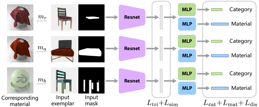
Figure 4. Material prediction network used in our work. During training, we use a triplet network composed of ResNets with shared weights (middle) to learn to embed the input images into a feature space that reflects the perceptual similarity of the materials in the images (left), and then we further learn two classifiers based on the feature space to predict the overall material category and material label (right). After training, the network can be used to predict the material category and label for a single input exemplar and selected part. The diagram also indicates the terms of the loss function used for training each part of the network.

The loss function for training our material prediction network is defined as follows:

(5) $$L_{p}=L_{\text{metric}}+L_{\text{class}},$$

where $L_{\text{metric}}$ is the metric learning loss to ensure the embedded features reflect the perceptual distance, and $L_{\text{class}}$ is the loss defined on the final material assignment to make sure it is similar to the ground truth.

4.2.1. Metric learning loss.

The metric learning loss $L_{\text{metric}}$ is adapted from the work of Lagunas et al. (2019b), and composed of two losses defined on material triplets, where each triplet given to the network consists of a reference image $r$ with material $m_{r}$, one positive example $a$ with material $m_{a}$, and one negative example $b$ with material $m_{b}$. The metric learning loss is defined as:

(6) $$L_{\text{metric}}=\alpha_{1}L_{\text{tri}}+\alpha_{2}L_{\text{sim}},$$

where $L_{\text{tri}}$ is the triplet loss that seeks to bring similar materials $r$ and $a$ closer together in the feature space and repel dissimilar materials $b$, and $L_{\text{sim}}$ is the similarity loss that further maximizes the log-likelihood of the model choosing $a$ to be closer to $r$ than $b$.

The triplet loss is defined as follows (Lagunas et al., 2019b):

(7) $$L_{\text{tri}}(r,a,b)=\frac{1}{|B^{A}|}\sum_{(r,a,b)\in B^{A}}\left[\lVert f_{r}-f_{a}\rVert_{2}^{2}-\lVert f_{r}-f_{b}\rVert_{2}^{2}+\mu\right]_{+},$$

where $[x]_{+}=\max(0,x)$, $f_{x}$ is the feature vector of $x$, $\mu$ is the margin which specifies how much we would like to separate the samples in the feature space, and $B^{A}$ is the set of triplets that take part in the training.

The similarity loss is defined as follows (Lagunas et al., 2019b):

(8) $$L_{\text{sim}}=-\frac{1}{|B^{A}|}\sum_{(r,a,b)\in B^{A}}\log\frac{s_{ra}}{s_{ra}+s_{rb}},$$

where $s_{ra}=\dfrac{1}{1+\lVert f_{r}-f_{a}\rVert_{2}^{2}}$ and $s_{rb}=\dfrac{1}{1+\lVert f_{r}-f_{b}\rVert_{2}^{2}}$.

To construct the training triplets $B^{A}$, we first generate a set of pre-sampled material triplets $A^{M}$. To generate $A^{M}$, we randomly sample a reference material $m_{r}$, a random sampled positive material $m_{a}$ which is of the same category as $m_{r}$, and a negative material $m_{b}$ which is of a different category than $m_{r}$. The material $m_{b}$ is sampled so that it has a larger perceptual distance to $m_{r}$ than $m_{a}$, i.e., $D(m_{r},m_{b})>D(m_{r},m_{a})$, but also has a distance smaller than the distances to all other materials of all different categories, i.e., $D(m_{r},m_{b})<D(m_{r},m_{x})$, where $m_{x}$ is any material of a category other than the category of $m_{r}$. Then $B^{A}$ is defined as:

(9) $$B^{A}=\left\{(r,a,b)\mid(m_{r},m_{a},m_{b})\in A^{M}\wedge(r,a,b)\in B\right\},$$

where $B$ is the current training batch. Thus, $B^{A}$ is the set of all triplets of images in $B$ whose corresponding material labels appear as triplets in $A^{M}$.

4.2.2. Classification loss.

The classification loss $L_{\text{class}}$ for training our material prediction network is defined as follows:

(10) $$L_{\text{class}}=\alpha_{3}{\color[rgb]{0,0,0}\textbf{}L_{\text{cat}}}+\alpha_{4}L_{\text{mat}}+\alpha_{5}L_{\text{dis}},$$

where $L_{\text{cat}}$ and $L_{\text{mat}}$ are the cross entropy losses defined by Park et al. (2018) for material category and label classification, and $L_{\text{dis}}$ is the distance loss to minimize the perceptual distance between the predicted material and the ground truth material:

(11) $$L_{\text{dis}}(m_{p},m_{gt})=m_{p}^{T}D_{\text{idx}(m_{gt})},$$

where $m_{p}$ and $m_{gt}$ are the predicted and ground truth material labels, represented as $n$-dimensional column vectors where $n$ is the size of the material dataset. Specifically, these vectors are one-hot vectors for the ground truth labels, and probability vectors for predicted labels. $D_{i}$ represents the $i$-th column of the matrix $D$, $\text{idx}(m_{gt})$ is the index of the ground truth material and thus $D_{\text{idx}(m_{gt})}$ encodes the perceptual distance of $m_{gt}$ to all other materials.

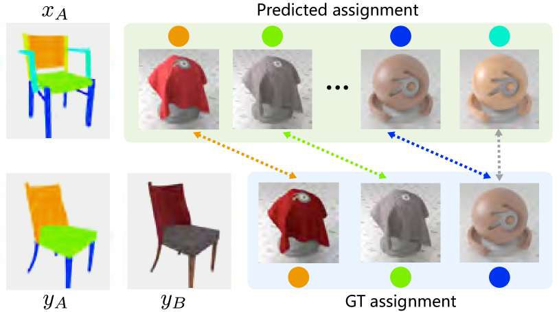
Figure 5. Method for constructing the ground truth part material assignment for (color, segmentation) pairs generated by the image translation network. This ground truth is used for computing the loss of the material prediction network. When defining the ground truth of $O_{s}$, for corresponding parts that exist in $P_{s}$, the ground truth assignment is the corresponding part material indicated by the colored arrows. For parts that do not exist in $P_{s}$ (cyan material on the top-right), the ground truth assignment is the part material in the ground truth assignment with minimal perceptual distance to the predicted material, indicated by the gray arrow.

4.3. Material transfer

As illustrated in Figure 2, the entire pipeline for material transfer from the given photo exemplar to the 3D shape consists of two key steps, i.e., image translation and material prediction. We first pre-train the image translation and material prediction networks separately, and then fine-tune the material prediction network to provide consistent part material assignments for two (color, segmentation) image pairs, i.e., (${\color[rgb]{0,0,0}\textbf{}P_{c}},\hat{P}_{s}$) and (${\color[rgb]{0,0,0}\textbf{}\hat{O}_{c}},O_{s}$). Note that the two (color, segmentation) image pairs have different input features, since the translated color $\hat{O}_{c}$ may be noisy and the translated segmentation $\hat{P}_{s}$ can be inaccurate. Thus, we fine-tune two versions of the material prediction network for each of the two pairs separately, and then use a consistency loss to enforce a consistent part assignment.

Moreover, when training the material prediction network alone, the required training data with ground truth can be easily generated given the dataset we collected. However, it is challenging to create ground truth data for training the entire pipeline together, since we require corresponding translated (color, segmentation) image pairs, but these are difficult to create due to the existence of missaligned structures in the images and unmatched semantic parts. We use different methods to determine the ground truth for the two different types of translated (color, segmentation) image pairs.

4.3.1. Fine-tuning with translated color.

The synthetic exemplar $P_{c}$ has the corresponding ground truth semantic mask $P_{s}$ and part material assignment $\{s_{P}^{i},m_{P}^{i}\}_{i=1}^{n_{P}}$, where $s_{P}^{i}$ is a part with a specific semantic label. For the given projection $O_{s}$ with semantic parts $\{s_{O}^{j}\}_{j=1}^{n_{O}}$, since the paired colored image $\hat{O}_{c}$ is translated from $P_{c}$ and the goal is to transfer the part material based on the semantic mapping between $P_{s}$ and $O_{s}$, we set the ground truth part material assignment for $\hat{O}_{c}$ to be $\{p_{O}^{j},m_{O}^{j}\}_{j=1}^{n_{O}}$, where $m_{O}^{j}=m_{P}^{i}$ if there exists some $i$ such that $s_{O}^{j}=s_{P}^{i}$, and use only the set of parts with corresponding material assignment to fine-tune the material prediction network. Otherwise, we set the ground truth as the material from the set $\{m_{y}^{i}\}$ with minimal perceptual distance to the predicted material. Figure 5 illustrates this method.

4.3.2. Fine-tuning with translated segmentation.

For (${\color[rgb]{0,0,0}\textbf{}P_{c}},\hat{P}_{s}$) pairs, as the generated segmentation $\hat{P}_{s}$ is translated from $O_{s}$, when $P_{c}$ has parts that do not exist in $O_{s}$, the translated $\hat{P}_{s}$ may become under-segmented, where some semantic parts could cover regions with multiple different materials and thus cannot be assigned with a single material label as ground truth. To overcome this problem, we oversegment the exemplar $P_{c}$ and use its intersection with the translated segmentation $\hat{P}_{s}$ as the part masks. More specifically, each semantic part $s_{\hat{P}}^{i}$ of $\hat{P}_{s}$ is subdivided into a set of smaller regions $\{s_{\hat{P}}^{\{i,t\}}\}_{t=1}^{n_{i}}$, and each over-segment $s_{\hat{P}}$ is paired with the corresponding colored region in $P_{c}$ to be the input to the material prediction network. The dominant material of the paired color region is taken as the ground truth. We find that, with the over-segmentation, the part materials become more consistent, and the training data obtained is more reliable for fine-tuning the material prediction network.

4.3.3. Fine-tuning with consistency loss.

To ensure that the material assignments predicted from the two image pairs obtained by the image translation are consistent during the fine-tuning, we add a consistency loss $L_{c}$. Note that for (${\color[rgb]{0,0,0}\textbf{}P_{c}},\hat{P}_{s}$) pairs, each semantic part $s_{\hat{P}}^{i}$ may be subdivided into multiple regions $\{s_{\hat{P}}^{\{i,t\}}\}_{t=1}^{n_{i}}$ for material prediction, as explained above, and thus there may exist a one-to-many mapping between semantic parts from (${\color[rgb]{0,0,0}\textbf{}\hat{O}_{c}},O_{s}$) and (${\color[rgb]{0,0,0}\textbf{}P_{c}},\hat{P}_{s}$). Our goal is to minimize the weighted average perceptual distance for the material predicted for the parts from the two different pairs but with the same semantics. More specifically, the consistency loss is defined as:

(12) $$L_{c}=\sum_{i_{k},j_{k}}\left(\sum_{t=1}^{n_{j_{k}}}\omega_{t}L_{\text{dis}}(m_{O}^{i_{k}},m_{P}^{\{j_{k},t\}})\right),$$

where $\{i_{k},j_{k}\}$ is the set of matched part indices between two pairs, $n_{j_{k}}$ is the number of sub-regions of semantic parts $s_{\hat{P}}^{j_{k}}$ of $\hat{P}_{s}$ after over-segmentation, $m_{O}^{i_{k}}$ and $m_{P}^{\{j_{k},t\}}$ are the material prediction results for the corresponding parts of pair (${\color[rgb]{0,0,0}\textbf{}\hat{O}_{c}},O_{s}$) and pair (${\color[rgb]{0,0,0}\textbf{}P_{c}},\hat{P}_{s}$), respectively, $L_{\text{dis}}$ is the perceptual distance loss defined in Eq. 11, and $\omega_{t}$ is the normalized weight over part $s_{\hat{P}}^{j_{k}}$ based on the area of subdivided regions.

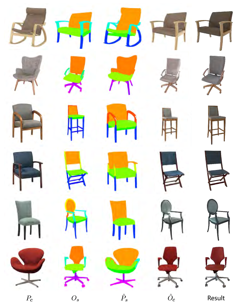
Figure 7. Sample of results showing the steps of our method: Input exemplar and segmentation (left), segmentation and color translation (middle), and material transfer result (right). Rows 1-2: shapes with similar number of parts but with different structure; Rows 3-4: target shapes with fewer parts; Rows 5-6: target shapes with more parts.

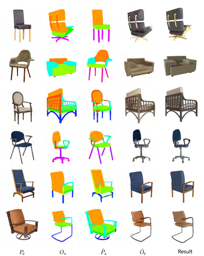
Figure 8. Our material transfer method is robust and generates high-quality results even in cases of incorrect camera pose estimation. The figure shows the input exemplar and segmentation (left two columns), segmentation and color translation (middle two columns), and the material transfer result (right column).

5. Results and Evaluation

In this section, we first present qualitative results and comparisons of our method. Then, we perform a set of experiments to evaluate the results and different components of our method in a quantitative manner, showing the importance of each component. The set up for training our method can be found in the supplementary material.

5.1. Qualitative results

Figure 1 shows a gallery of results generated with our method, to illustrate that our material transfer method can be used to generate collections with a variety of PhotoShapes. All these results were generated from in-the-wild photos with foreground extracted using automatic segmentation. Specifically, we used the Kaleido background removal plugin from Photoshop (version 2.0.6).

Figure 7 shows a sample of results obtained with our method, where we show the input exemplar and segmentation on the left, translated segmentation and color images in the middle, and final material transfer result on the right. When inspecting these results, we see that the method is able to handle chairs with different structure and geometry. For example, the method successfully transfers the materials from a square to a round back (row 5), exchanges materials between legs with different topologies (rows 2 and 3), armrests with different topologies (row 2), and backs with different topologies (row 4). The presence of extra parts such as armrests or leg supports does not affect the transfer results (rows 3 and 6). In addition, the method is also successful in assigning materials to chairs with arm rests even though the exemplars do not have this part (rows 5 and 6). In these cases, the method is able to infer the material from the semantic labels of the parts. Note that previous methods that assume sufficient similarity between the shape and exemplar would fail in most of these difficult cases.

Figure 8 shows results obtained with incorrect camera pose estimation, where the most common error in the camera pose estimation step is a type of symmetric reflection of the correct pose. We find that our method still generates high-quality results despite incorrect camera pose estimation and imperfect translated segmentation $\hat{P}_{s}$. Since our goal is to estimate the material for each semantic part in $O_{s}$, as long as enough parts are visible in the selected pose, the image translation method is able to predict proper materials for the target parts.

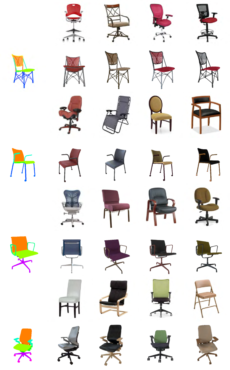
Figure 9. Example results where the material of different exemplars (columns) is transferred to the same shape (rows). For better comparison, we rotate the 3D shape to the same view as the exemplar.

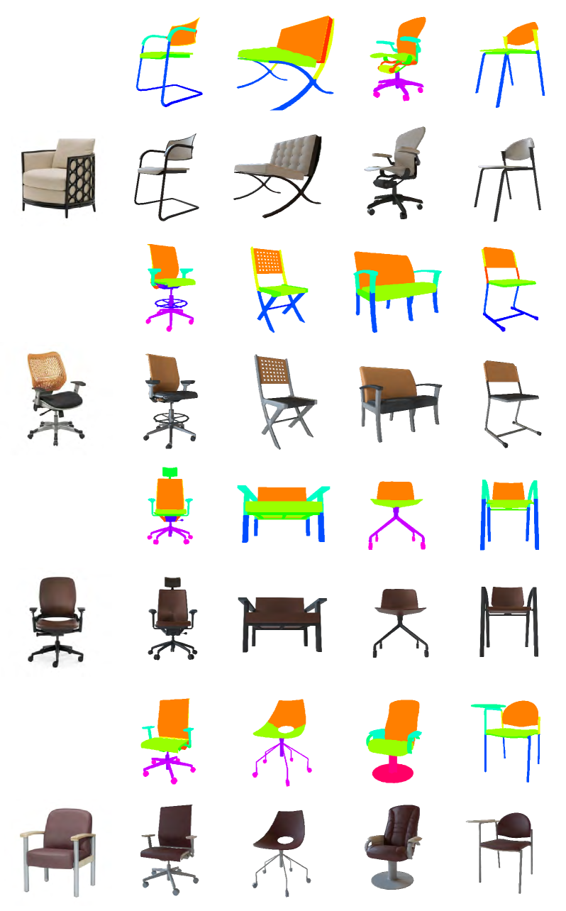
Figure 10. Example results where the material of the same exemplar (rows) is transferred to different shapes (columns). For better comparison, we rotate the 3D shapes to the same view as the exemplar.

Moreover, Figure 9 shows examples of results where we fix a 3D shape and transfer the materials from different exemplars to the same shape. We see that the method can transfer materials from different categories to the same shape, such as woods, metals, and leathers. Figure 10 shows the complementary scenario where we fix an exemplar and transfer it to different 3D shapes. With these two comparisons, we see again that the structure and geometry of the exemplar does not need to perfectly match those of the 3D shape, where both the shape and exemplar can have additional parts that do not appear in the other object. The method is robust to these shape differences and thus can be applied to a great variety of objects. In addition, we see from these two comparisons that the user can choose a specific exemplar and 3D shape for the material assignment. Previous methods are able to transfer materials only when the exemplar and shape are sufficiently similar, implying that the user has less control over the input.

5.2. Qualitative evaluation

As there is no ground truth for the material transfer results due to the difficulty involved in its creation, we conduct a user study to evaluate the quality of the results generated by our method comparing to the results of baseline methods.

Baseline methods.

We compare our method to two different baselines that solve the same problem as our method with different strategies.

The first baseline is the PhotoShape method of Park et al. (2018), which is the previous work most related to our method. We run PhotoShape using the authors’ code for shape-image alignment, but our network for material prediction, since we show in Section 5.3 that the material prediction accuracy of our method is higher.

The second baseline, denoted as PhotoShape+, is a simplified version of our method, which incorporates a segmentation network with the shape-image alignment proposed in PhotoShape (Park et al., 2018). More specifically, instead of using a translation network, we train an image segmentation network to first get the semantic segmentation of the photo exemplar. Then, we provide the photo exemplar and each of its predicted semantic parts as input to our material prediction network to obtain the part material labels. We use DeepLabv3+ (Chen et al., 2018) as the segmentation network. Note that for this baseline, we can only assign materials to shape parts that have corresponding parts in the photo exemplar. It may be possible to use heuristics for assigning materials to unmatched parts, for example, by renormalizing the predicted distribution using the semantic labels that exist in the 3D shape, or assigning the semantic labels based on similarities to missing parts. However, we found that renormalization does not lead to meaningful results for most of the cases, and thus it is difficult to justify using handcrafted equivalence rules for different parts. Thus, for any unmatched part, we deform $O_{s}$ to align it with the photo exemplar $P_{c}$ using the shape-image alignment method proposed by Park et al. (2018), and then assign the material of the corresponding region in the photo exemplar to the part to get a complete material assignment for the given shape.

User study.

Before starting the user study, we explain the goal of material transfer to the users. The specific wording used in the instructions and in the questions is provided in the supplementary material. Then, we ask the users multiple questions where we show the result of one of the baselines and our method, in random order, and ask the user to select which result they think is better. The user can select either one of the two results or a “not sure” option.

To conduct the user study, we collected 300 sets of results by sampling exemplar images and 3D shapes from our dataset, and provided these as input to the different methods to obtain three different transfer results. After that, we compare our method to each baseline separately, which results in 600 questions. We asked 12 participants to do the user study, all of whom are graduate students in computer science. We collected 150 answers from each participant and thus 1,800 answers in total, with each of the 600 questions having answers from three different participants. For each question, we take the answer selected by the majority of the participants as the final answer, and consider the answer to be “not sure” if there is no agreement among the answers when we get three different answers.

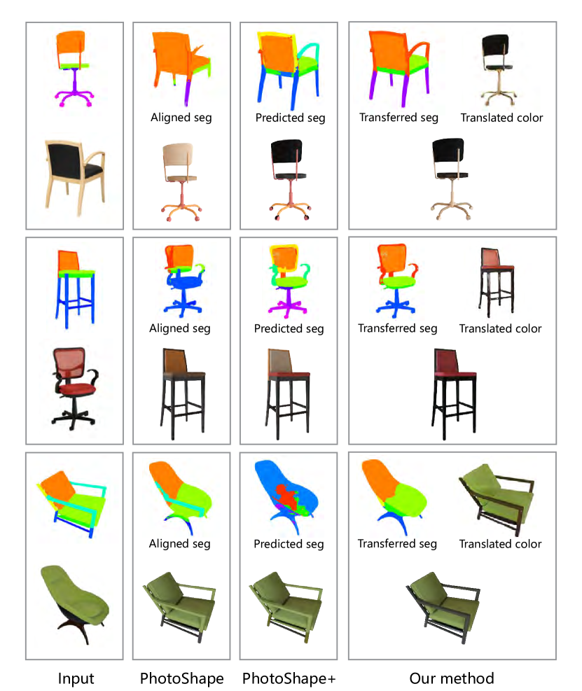
Figure 11. Comparison of our method to two baselines. Note how the intermediate results of our method build a better correspondence between the input segmentation and exemplar, and how the final results of our method better resemble the exemplar.

Results.

When comparing to PhotoShape, the vote percentages for the options “PhotoShape/ours/not sure” are $19.3\%/70.7\%/10\%$, and when comparing to PhotoShape+, the vote percentages for the options “PhotoShape+/ours/not sure” are $21.3\%/62.7\%/16\%$. We see that our method was selected much more frequently than other methods as having the best result, and we can also conclude that there must be a noticeable improvement in our results compared to other methods, given that the number of “not sure” votes is small. To evaluate in a quantitative manner how well the final results obtained by different methods resemble the input photo exemplars, we also compute the Fréchet Inception Distance (FID) (Heusel et al., 2017) between the images rendered from the predicted camera views and the input photo exemplars, as in the work of Oechsle et al. (2019). The FIDs for “PhotoShape/PhotoShape+/ours” are $58.66/58.16/57.33$, which are consistent with the human judgment.

In Figure 11, we present a visual comparison of our method to the two baselines on a few examples to provide more insight on the user study results. For each example, we show the intermediate results of all the methods for more detailed comparison. More specifically, we show the aligned segmentation for PhotoShape, additional predicted segmentation for PhotoShape+, and both translated segmentation and color for our method.

For example, when analyzing the results shown in the first row of the figure, we see that since the structures of the input 3D shape and the shape in the exemplar photo are quite different, especially with many thin parts, the segmentation obtained by the shape-image alignment method in PhotoShape is noisy, which results in image regions consisting of several different materials that correspond to a single semantic part. Thus, this segmentation leads to unreliable material prediction for parts like the back and seat of the chair. Since PhotoShape+ relies on a more accurate semantic segmentation predicted by the segmentation network, PhotoShape+ builds a correct, clean correspondence between the semantic parts and the corresponding regions in the exemplar photo, and transfers the correct material to the seat and back of the chair. However, since the legs of the swivel chair have thin parts that do not exist in the exemplar shape, the material assignment is unsatisfactory, since the corresponding materials are assigned based on the alignment results obtained in PhotoShape, which are combined together to provide the final result for PhotoShape+. Comparing to these two baselines, our method translates the segmentation from the input shape to the exemplar smoothly and in turn provides much better material assignments in the final results. Similar results can be found for the example shown in the second row.

For the result shown in the last row, when the exemplar has a smaller number of semantic parts than the 3D shape, the shape-image alignment method in PhotoShape assigns materials predicted for parts with different semantics, which leads to unrealistic results, e.g., the green armrest. Moreover, as the chair in this exemplar photo has an irregular shape, the segmentation network used in PhotoShape+ outputs highly incorrect results which lead to incorrect material assignments for parts like legs. In contrast, our method benefits from the image translation to obtain a more accurate segmentation, and synthesizes a realistic color image for material prediction for unmatched parts, i.e., the armrest, which together leads to the result that better resembles the exemplar.

Overall, our results better conform to the materials seen in the input exemplar, both in category and albedo. We see significant improvement especially when the matching parts have large geometric differences, or with missing parts.

5.3. Quantitative evaluation

In this section, we conduct a quantitative evaluation of the material prediction network with synthetic image pairs, which provide ground truth material and category labels that we can use for computing accuracy measures.

We evaluate the quality of the material labeling compared to the ground truth with three measures: 1 and 2. Material and category accuracies (Mat-acc, Cat-acc, respectively), computed as the classification accuracy (number of correctly assigned labels / total number of parts), where the goal is to maximize the accuracy; 3. Material perceptual distance (Mat-dis), computed with the L2-lab distance (Sun et al., 2017), where the goal is to minimize the distance between the ground truth and assigned materials.

To prepare the synthetic (color, segmentation) pairs, we first create (color, segmentation) tuples by rendering the 3D shapes in our dataset from different views and extracting the corresponding semantic projections for each view based on the part segmentation of the shapes. Then, for each rendered image, we use the camera pose prediction network to predict the camera parameters of the image. To generate a second (color, segmentation) tuple corresponding to the rendered image, we arbitrarily select another shape from the dataset and generate its rendering and semantic projection from the predicted view. This procedure provides us with translated (color, segmentation) image pairs. We divided the image pairs into training and test sets. The details about the ground truth material assignment, synthetic image generation, and exact data division for training and testing can be found in the supplementary material.

Note that the material prediction network is first trained using synthetic (color, segmentation) image pairs, which are obtained by directly rendering the 3D shapes in our dataset with assigned materials from different views, and then fine-tuned with translated (color, segmentation) image pairs obtained with our image translation method by taking an exemplar color image and a 3D shape as input. We have ground truth material labels for all the synthetic image pairs, but only partial ground truth for translated images pairs, which is derived from the semantic correspondence between the input exemplar and 3D shape as discussed in Section 4.3. Thus, we perform two ablation studies to evaluate these two fine-tuning steps separately to demonstrate the importance of considering the perceptual similarity for material prediction and the importance of ensuring the consistency between the prediction results of two translated image pairs for material transfer.

Table 1. Comparison of the material prediction network trained with different losses (Settings 1–3 in the text). Note the better performance of the full loss $L_{\text{class}}+L_{\text{metric}}$, where $L_{\text{class}}={\color[rgb]{0,0,0}\textbf{}L_{\text{cat}}}+L_{\text{mat}}+L_{\text{dist}}$ is the classification loss and $L_{\text{metric}}$ is the metric learning loss.

Loss	Mat-acc ($\uparrow$)	Sub-acc($\uparrow$)	Mat-dis ($\downarrow$)
${\color[rgb]{0,0,0}\textbf{}L_{\text{cat}}}+L_{\text{mat}}$	57.53%	81.89%	7.69
${\color[rgb]{0,0,0}\textbf{}L_{\text{cat}}}+L_{\text{mat}}+L_{\text{dist}}$	61.56%	84.30%	6.38
$L_{\text{class}}+L_{\text{metric}}$	71.62%	86.49%	4.66

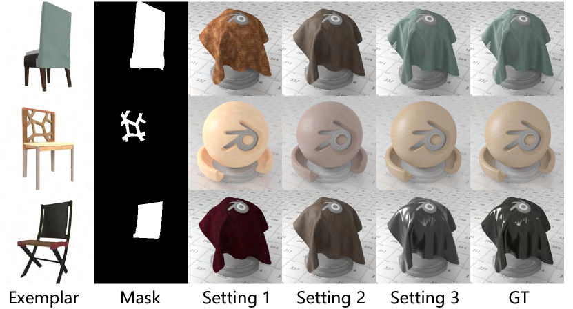
Figure 12. Examples comparing the material prediction network learned with different settings of the loss function. We use Setting 3.

Importance of considering perceptual similarity. We first use synthesized (color, segmentation) image pairs to compare the material prediction network learned with and without the perceptual similarity, and also evaluate the learning of the perceptual similarity with different forms of the loss function. We evaluate the following settings:
$\bullet$ Setting 1: the prediction network trained without the perceptual distance loss (the same setting as Park et al. (2018)). This corresponds to training the network with the loss ${\color[rgb]{0,0,0}\textbf{}L_{\text{cat}}}+L_{\text{mat}}$;
$\bullet$ Setting 2: directly adding the perceptual distance loss to the classification loss, i.e., using ${\color[rgb]{0,0,0}\textbf{}L_{\text{cat}}}+L_{\text{mat}}+L_{\text{dis}}$;
$\bullet$ Setting 3: using the perceptual distance measure in a softer way to learn a perception-aware feature space first, i.e., using the distance matrix to sample triplets to perform metric learning, and then fine-tuning the network to perform the classification with the same loss as Setting 2. Thus, Setting 3 uses all the terms of the loss function, i.e., $L_{\text{metric}}+L_{\text{class}}$, and corresponds to the setting used in our method.

The comparison is shown in Table 1, while a visual comparison is shown in Figure 12. With this study, we confirm that the use of the perceptual loss and the full loss function provide the best material assignments, where the accuracy increases with the addition of each term of the loss function. In Figure 12, we see the same gradual improvement with the addition of more terms of the loss.

Importance of fine-tuning with consistency loss. For the two (color, segmentation) image pairs generated by the image translation step, i.e., (${\color[rgb]{0,0,0}\textbf{}P_{c}},\hat{P}_{s}$) and (${\color[rgb]{0,0,0}\textbf{}\hat{O}_{c}},O_{s}$), we show the necessity of the fine-tuning process described in Section 4.3, which fine-tunes two separate networks and also uses a consistency loss. We compare the material prediction accuracy before and after fine-tuning for both pairs in Table 2. Figure 13 shows a visual comparison of results.

Table 2. Comparison of the prediction accuracy for the translated image pairs before and after fine-tuning. Note the better performance with fine-tuning for both (${\color[rgb]{0,0,0}\textbf{}P_{c}},\hat{P}_{s}$) and (${\color[rgb]{0,0,0}\textbf{}\hat{O}_{c}},O_{s}$).

Data	Fine-tune	Mat-acc ($\uparrow$)	Sub-acc($\uparrow$)	Mat-dis ($\downarrow$)
(${\color[rgb]{0,0,0}\textbf{}P_{c}},\hat{P}_{s}$)	N	64.87%	85.26%	8.31
	Y	79.17%	90.41%	5.24
(${\color[rgb]{0,0,0}\textbf{}\hat{O}_{c}},O_{s}$)	N	10.26%	43.83%	16.88
	Y	24.18%	59.71%	12.10
	Y + $L_{c}$	26.95%	62.32%	11.17

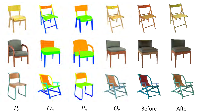
Figure 13. Comparison of results before and after fine-tuning. Note how the results better resemble the exemplars $P_{t}$ when fine-tuning is used.

When comparing the results from two different image pairs, we see that the prediction accuracy of the (${\color[rgb]{0,0,0}\textbf{}\hat{O}_{c}},O_{s}$) pairs is much lower than that of (${\color[rgb]{0,0,0}\textbf{}P_{c}},\hat{P}_{s}$) pairs. The reason is that the material prediction network takes a color image and a mask as input, and the prediction results are highly determined by the quality of the color image, while the material prediction network is trained on rendered data, which is quite different from the translated colored $\hat{O}_{c}$. However, note that for parts that can be found in $\hat{P}_{s}$, we use the prediction result for the (${\color[rgb]{0,0,0}\textbf{}P_{c}},\hat{P}_{s}$) pair, and the prediction results for (${\color[rgb]{0,0,0}\textbf{}\hat{O}_{c}},O_{s}$) are only used for unmatched semantic parts. We can see that by adding the consistency loss $L_{c}$ to ensure consistent prediction results for the corresponding two image pairs, the results are improved. Our current setting shown in the last row obtains the best results on all the three metrics.

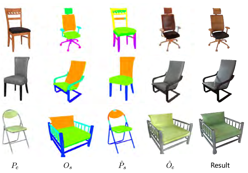
Figure 14. Representative failure cases of our method: semantic mismatch between exemplar and shape (Row 1), incorrect material inference (Row 2), and insufficient variety of the material dataset (Row 3).

5.4. Failure cases

Figure 14 shows example results that represent the main failure modes of our method. We identify three main failures cases: 1) The image translation and material assignment are correct. However, the result does not make sense due to a semantic mismatch between the exemplar and the shape. For example, in the first row of the figure, a wooden material is assigned to the back of a swivel chair. Such type of category assignment is rarely found in real-world designs. 2) The material prediction network predicts a visually similar but incorrect material category, such as the seat of the chair shown in the second row, where a metal material is assigned instead of a fabric material. Note that the material predicted for the back is more accurate even though the materials presented in the exemplar photo are the same for the seat and the back. This incorrect material prediction is caused by different reflectance effects on different parts. Inconsistent prediction results for related parts are due to the independent per-part material prediction of our method. 3) The material assignment does not match perfectly with the exemplar, due to insufficient variety of materials in the dataset. In the third row of the figure, the green materials have a slightly different hue.

5.5. Application to other categories of shapes

To demonstrate that our method is general and can also be applied to categories other than chairs, which have been the sole focus of some of the previous work (Park et al., 2018), we also show results for other categories of shapes in Figure 15. To obtain these results, we retrain the image translation network as different categories have different semantics. However, the network is trained with the same set of hyperparameters. Moreover, we use exactly the same material predictor network that was trained on the chairs.

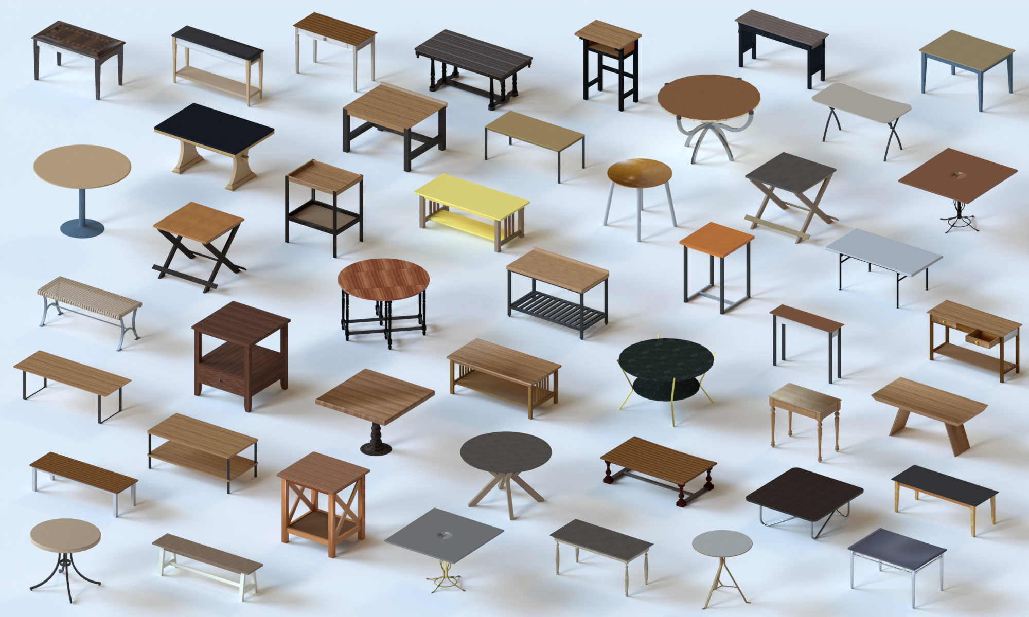
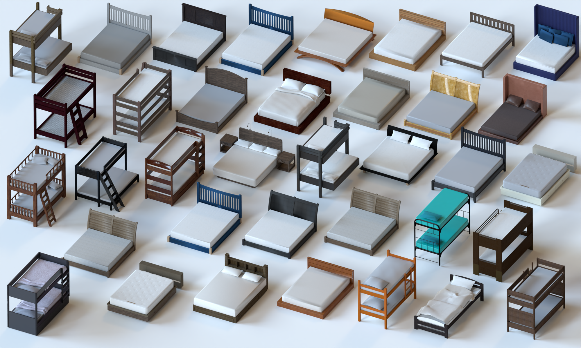
Figure 15. Results for other categories of shapes to demonstrate the generality of our method.

6. Discussion and Future Work

We presented a method for material transfer from photo exemplars to 3D shapes, based on a combination of image translation and material assignment according to perceptual similarity. We showed with qualitative and quantitative evaluations that, compared to other baseline methods, our method is more robust in handling objects with diverse structures and provides shapes with materials that are closer in appearance to the provided exemplars. As a consequence, given large collections of 3D shapes and exemplars, our method can automatically create a corresponding large collection of shapes with realistic materials. In addition, given a specific 3D shape and exemplar, our method is more likely to succeed in transferring the material from the exemplar to the shape than previous works, given the improvements that we introduced with our method.

Limitations.

Our method has certain limitations, such as the ones that cause the failure cases discussed in Figure 14. For example, our method assigns materials from a database to best match the exemplar. Thus, there could still be some discrepancies between the exemplar and the appearance of the resulting 3D shape. Moreover, all the synthetic training images are rendered using the same illumination settings. Thus, our method may incorrectly predict a material if the photo exemplar is taken under quite different lighting. Also, currently our material prediction method is applied on each semantic part separately without considering the global consistency of the materials combined together in a single shape, which may lead to unrealistic rendering results.

Future work.

One direction for future work is to address the limitations summarized in Figure 14. Training the networks with more images rendered under different illumination settings may improve the robustness of the method. However, the additional data may also conflict with our losses that use the perceptual similarity, since it is unclear whether perception changes are caused solely by the material itself or also by the lighting. Thus, it would be interesting to explore ways to disentangle the effects of lighting from the material prediction and assignment. Moreover, we believe that designing a network that predicts the materials for all the parts at once while ensuring their consistency is worth exploring.

Our image translation network is currently class specific. Thus, one direction for future work would be to experiment with a class-independent translation network. Finally, it would be interesting to combine our material assignment method with large collections of high-quality textures or texture generation methods, in order to handle exemplars with more complex textures, such as geometric patterns. The use of recent inverse texture modeling approaches would be a promising approach for exploring this research direction (Hu et al., 2019).

7. ACKNOWLEDGEMENTS

We thank the anonymous reviewers for their valuable comments. This work was supported in parts by NSFC (61872250, U2001206, U21B2023, 62161146005), GD Talent Plan (2019JC05X328), GD Natural Science Foundation (2021B1515020085), DEGP Key Project (2018KZDXM058, 2020SFKC059), Shenzhen Science and Technology Program (RCYX20210609103121030, RCJC20200714114435012, JCYJ20210324120213036), the Natural Sciences and Engineering Research Council of Canada (NSERC), and Guangdong Laboratory of Artificial Intelligence and Digital Economy (SZ).

References

- (1)
- Bell et al. (2013) Sean Bell, Paul Upchurch, Noah Snavely, and Kavita Bala. 2013. OpenSurfaces: A Richly Annotated Catalog of Surface Appearance. ACM Trans. on Graphics (Proc. SIGGRAPH) 32, 4 (2013), 111:1–17.
- Bell et al. (2015) Sean Bell, Paul Upchurch, Noah Snavely, and Kavita Bala. 2015. Material Recognition in the Wild With the Materials in Context Database. In Proc. IEEE Conf. on Computer Vision & Pattern Recognition.
- Chen et al. (2018) Liang-Chieh Chen, Yukun Zhu, George Papandreou, Florian Schroff, and Hartwig Adam. 2018. Encoder-decoder with atrous separable convolution for semantic image segmentation. In Proceedings of the European conference on computer vision (ECCV). 801–818.
- Chen and Koltun (2017) Qifeng Chen and Vladlen Koltun. 2017. Photographic Image Synthesis With Cascaded Refinement Networks. In Proc. Int. Conf. on Computer Vision.
- Chen and Zhang (2019) Zhiqin Chen and Hao Zhang. 2019. Learning Implicit Fields for Generative Shape Modeling. In Proc. IEEE Conf. on Computer Vision & Pattern Recognition. 5939–5948.
- Chibane et al. (2020) Julian Chibane, Aymen Mir, and Gerard Pons-Moll. 2020. Neural Unsigned Distance Fields for Implicit Function Learning. In Advances in Neural Information Processing Systems (NeurIPS).
- Delanoy et al. (2018) Johanna Delanoy, Mathieu Aubry, Phillip Isola, Alexei A. Efros, and Adrien Bousseau. 2018. 3D Sketching Using Multi-View Deep Volumetric Prediction. In Proc. ACM Comput. Graph. Interact. Tech. 21:1–15.
- Deng et al. (2009) Jia Deng, Wei Dong, Richard Socher, Li-Jia Li, Kai Li, and Li Fei-Fei. 2009. Imagenet: A large-scale hierarchical image database. In 2009 IEEE conference on computer vision and pattern recognition. Ieee, 248–255.
- Guarnera et al. (2016) D. Guarnera, G. C. Guarnera, A. Ghosh, C. Denk, and M. Glencross. 2016. BRDF Representation and Acquisition. In Proc. Eurographics State of the Art Reports. Eurographics Association, 625–650.
- Han et al. (2021) Xian-Feng Han, Hamid Laga, and Mohammed Bennamoun. 2021. Image-Based 3D Object Reconstruction: State-of-the-Art and Trends in the Deep Learning Era. IEEE Trans. Pattern Analysis & Machine Intelligence 43, 5 (2021), 1578–1604.
- Havran et al. (2016) Vlastimil Havran, Jiri Filip, and Karol Myszkowski. 2016. Perceptually motivated BRDF comparison using single image. In Computer graphics forum, Vol. 35. Wiley Online Library, 1–12.
- He et al. (2016) Kaiming He, Xiangyu Zhang, Shaoqing Ren, and Jian Sun. 2016. Deep residual learning for image recognition. In Proceedings of the IEEE conference on computer vision and pattern recognition. 770–778.
- Heusel et al. (2017) Martin Heusel, Hubert Ramsauer, Thomas Unterthiner, Bernhard Nessler, and Sepp Hochreiter. 2017. Gans trained by a two time-scale update rule converge to a local nash equilibrium. Advances in neural information processing systems 30 (2017).
- Hoffer and Ailon (2015) Elad Hoffer and Nir Ailon. 2015. Deep metric learning using triplet network. In International workshop on similarity-based pattern recognition. Springer, 84–92.
- Hu et al. (2021) Tao Hu, Geng Lin, Zhizhong Han, and Matthias Zwicker. 2021. Learning to Generate Dense Point Clouds With Textures on Multiple Categories. In Proc. IEEE/CVF Winter Conference on Applications of Computer Vision (WACV). 2170–2179.
- Hu et al. (2019) Yiwei Hu, Julie Dorsey, and Holly Rushmeier. 2019. A Novel Framework for Inverse Procedural Texture Modeling. ACM Trans. on Graphics (Proc. SIGGRAPH Asia) 38, 6 (2019), 186:1–14.
- Huang et al. (2018b) Hui Huang, Ke Xie, Lin Ma, Dani Lischinski, Minglun Gong, Xin Tong, and Daniel Cohen-Or. 2018b. Appearance Modeling via Proxy-to-Image Alignment. ACM Trans. on Graphics 37, 1 (2018), 10:1–15.
- Huang et al. (2015) Qixing Huang, Hai Wang, and Vladlen Koltun. 2015. Single-view reconstruction via joint analysis of image and shape collections. ACM Transactions on Graphics (TOG) 34, 4 (2015), 1–10.
- Huang et al. (2018a) Xun Huang, Ming-Yu Liu, Serge Belongie, and Jan Kautz. 2018a. Multimodal Unsupervised Image-to-image Translation. In Proc. Euro. Conf. on Computer Vision.
- Isola et al. (2017) Phillip Isola, Jun-Yan Zhu, Tinghui Zhou, and Alexei A. Efros. 2017. Image-To-Image Translation With Conditional Adversarial Networks. In Proc. IEEE Conf. on Computer Vision & Pattern Recognition.
- Jain et al. (2012) Arjun Jain, Thorsten Thormählen, Tobias Ritschel, and Hans-Peter Seidel. 2012. Material memex: Automatic material suggestions for 3d objects. ACM Transactions on Graphics (TOG) 31, 6 (2012), 1–8.
- Ji et al. (2017) Mengqi Ji, Juergen Gall, Haitian Zheng, Yebin Liu, and Lu Fang. 2017. SurfaceNet: An End-To-End 3D Neural Network for Multiview Stereopsis. In Proc. Int. Conf. on Computer Vision. 2307–2315.
- Kalogerakis et al. (2017) Evangelos Kalogerakis, Melinos Averkiou, Subhransu Maji, and Siddhartha Chaudhuri. 2017. 3D Shape Segmentation with Projective Convolutional Networks. In Proc. IEEE Conf. on Computer Vision & Pattern Recognition.
- Lagunas et al. (2019a) Manuel Lagunas, Sandra Malpica, Ana Serrano, Elena Garces, Diego Gutierrez, and Belen Masia. 2019a. A Similarity Measure for Material Appearance. ACM Trans. on Graphics (Proc. SIGGRAPH) 38, 4 (2019), 135:1–12.
- Lagunas et al. (2019b) Manuel Lagunas, Sandra Malpica, Ana Serrano, Elena Garces, Diego Gutierrez, and Belen Masia. 2019b. A similarity measure for material appearance. ACM Transactions on Graphics (TOG) 38, 4 (2019), 1–12.
- Liu et al. (2017) Juncheng Liu, Zhouhui Lian, and Jianguo Xiao. 2017. Auto-Colorization of 3D Models from Images. In SIGGRAPH Asia 2017 Technical Briefs. 15:1–4.
- Mir et al. (2020) Aymen Mir, Thiemo Alldieck, and Gerard Pons-Moll. 2020. Learning to Transfer Texture from Clothing Images to 3D Humans. In Proc. IEEE Conf. on Computer Vision & Pattern Recognition. IEEE.
- Mo et al. (2019) Kaichun Mo, Shilin Zhu, Angel X Chang, Li Yi, Subarna Tripathi, Leonidas J Guibas, and Hao Su. 2019. Partnet: A large-scale benchmark for fine-grained and hierarchical part-level 3d object understanding. In Proceedings of the IEEE/CVF Conference on Computer Vision and Pattern Recognition. 909–918.
- Nguyen et al. (2012) Chuong H Nguyen, Tobias Ritschel, Karol Myszkowski, Elmar Eisemann, and Hans-Peter Seidel. 2012. 3D material style transfer. In Computer Graphics Forum, Vol. 31. Wiley Online Library, 431–438.
- Oechsle et al. (2019) Michael Oechsle, Lars Mescheder, Michael Niemeyer, Thilo Strauss, and Andreas Geiger. 2019. Texture fields: Learning texture representations in function space. In Proceedings of the IEEE/CVF International Conference on Computer Vision. 4531–4540.
- Park et al. (2019) Jeong Joon Park, Peter Florence, Julian Straub, Richard Newcombe, and Steven Lovegrove. 2019. DeepSDF: Learning Continuous Signed Distance Functions for Shape Representation. In Proc. IEEE Conf. on Computer Vision & Pattern Recognition. 165–174.
- Park et al. (2018) Keunhong Park, Konstantinos Rematas, Ali Farhadi, and Steven M Seitz. 2018. PhotoShape: photorealistic materials for large-scale shape collections. ACM Trans. on Graphics (Proc. SIGGRAPH Asia) 37, 6 (2018), 1–12.
- Pham et al. (2019) Quang-Hieu Pham, Thanh Nguyen, Binh-Son Hua, Gemma Roig, and Sai-Kit Yeung. 2019. JSIS3D: Joint Semantic-Instance Segmentation of 3D Point Clouds With Multi-Task Pointwise Networks and Multi-Value Conditional Random Fields. In Proc. IEEE Conf. on Computer Vision & Pattern Recognition.
- Raj et al. (2019) Amit Raj, Cusuh Ham, Connelly Barnes, Vladimir Kim, Jingwan Lu, and James Hays. 2019. Learning to Generate Textures on 3D Meshes. In Proc. IEEE Conf. on Computer Vision & Pattern Recognition.
- Rematas et al. (2016) Konstantinos Rematas, Chuong H Nguyen, Tobias Ritschel, Mario Fritz, and Tinne Tuytelaars. 2016. Novel views of objects from a single image. IEEE transactions on pattern analysis and machine intelligence 39, 8 (2016), 1576–1590.
- Schmidt et al. (2016) Thorsten-Walther Schmidt, Fabio Pellacini, Derek Nowrouzezahrai, Wojciech Jarosz, and Carsten Dachsbacher. 2016. State of the Art in Artistic Editing of Appearance, Lighting and Material. Computer Graphics Forum 35, 1 (2016), 216–233.
- Serrano et al. (2016) Ana Serrano, Diego Gutierrez, Karol Myszkowski, Hans-Peter Seidel, and Belen Masia. 2016. An Intuitive Control Space for Material Appearance. ACM Trans. on Graphics (Proc. SIGGRAPH Asia) 35, 6 (2016), 186:1–12.
- Su et al. (2014) Hao Su, Qixing Huang, Niloy J Mitra, Yangyan Li, and Leonidas Guibas. 2014. Estimating image depth using shape collections. ACM Transactions on Graphics (TOG) 33, 4 (2014), 1–11.
- Sun et al. (2017) Tiancheng Sun, Ana Serrano, Diego Gutierrez, and Belen Masia. 2017. Attribute-preserving gamut mapping of measured BRDFs. In Computer graphics forum, Vol. 36. Wiley Online Library, 47–54.
- Wang et al. (2016) Tuanfeng Y Wang, Hao Su, Qixing Huang, Jingwei Huang, Leonidas J Guibas, and Niloy J Mitra. 2016. Unsupervised texture transfer from images to model collections. ACM Trans. on Graphics (Proc. SIGGRAPH Asia) 35, 6 (2016), 177–1.
- Wu et al. (2017) Jiajun Wu, Yifan Wang, Tianfan Xue, Xingyuan Sun, William T Freeman, and Joshua B Tenenbaum. 2017. MarrNet: 3D Shape Reconstruction via 2.5D Sketches. In Proc. Conf. on Neural Information Processing Systems.
- Xu et al. (2019) Qiangeng Xu, Weiyue Wang, Duygu Ceylan, Radomir Mech, and Ulrich Neumann. 2019. Disn: Deep implicit surface network for high-quality single-view 3d reconstruction. arXiv preprint arXiv:1905.10711 (2019).
- Zhang et al. (2019) Bo Zhang, Mingming He, Jing Liao, Pedro V Sander, Lu Yuan, Amine Bermak, and Dong Chen. 2019. Deep exemplar-based video colorization. In Proc. IEEE Conf. on Computer Vision & Pattern Recognition. 8052–8061.
- Zhang et al. (2020) Pan Zhang, Bo Zhang, Dong Chen, Lu Yuan, and Fang Wen. 2020. Cross-Domain Correspondence Learning for Exemplar-Based Image Translation. In Proc. IEEE Conf. on Computer Vision & Pattern Recognition. IEEE.
- Zhu et al. (2018) Jie Zhu, Yanwen Guo, and Han Ma. 2018. A Data-Driven Approach for Furniture and Indoor Scene Colorization. IEEE Trans. Visualization & Computer Graphics 24, 9 (2018), 2473–2486.