Cherenkov Wakefield Radiation from an Open End of a Three-Layer Dielectric Capillary

Abstract

Modern trends in beam-driven radiation sources involve interaction of Cherenkov wakefields with open-ended circular waveguide structures having complicated dielectric lining, with a three-layer dielectric capillary recently offered for reducing the radiation divergency being a representative example Jiang et al. (2020). This paper presents rigorous approach allowing analytical description of electromagnetic processes occuring when the described structure is excited by single waveguide mode. In other words, corresponding canonical waveguide diffraction problem is considered in rigorous formulation. This is continuation of our recent paper Galyamin and Vorobev (2022) where a simpler case of a two-layer dielectric filling has been considered. Here we use the same analytical approach based on Wiener-Hopf-Fock technique and deal with more complicated case of a three-layer dielectric lining.

I Introduction

Dielectric-lined open-ended waveguide structures are considered nowadays as extremely promising for a variety of applications based on Cherenkov effect. In the context of the present paper, one can mention certain success in both dielectric wakefield acceleration Nanni et al. (2015); D. O’Shea et al. (2016); Wang et al. (2017); Jing et al. (2018); Hibberd et al. (2020); Tang et al. (2021)and development of high-power narrow-band radiation sources including those for Terahertz (THz) frequencies Galyamin et al. (2014); Ivanyan et al. (2014); Wang et al. (2018); Zhao et al. (2020). Typical structure for mentioned application is a dielectric capillary – a circular waveguide with a dielectric layer and axial channel for bunch passage. Recently, a promising three-layer modification of mentioned capillary has been offered which essentially reduces the width of the main radiation lobe and therefore enhances considerably the radiated power Jiang et al. (2020).

For further development of the discussed topics a rigorous approach allowing analytical investigation of both radiation from such open-ended capillary and its excitation by external source (bunch or electromagnetic pulse) would be extremely useful. In our recent papers Galyamin et al. (2021); Galyamin and Vorobev (2022), we have presented an efficient rigorous method for solving circular open-ended waveguide diffraction problems and illustrated this method using the case of uniform dielectric filling and a two-layer lining of the waveguide. Here we deal with more complicated geometry offered in Jiang et al. (2020) and internal excitation by single waveguide mode. The presented technique can be directly applied to the radiation of CR wakefield generated behind the moving charge in the form of a slow waveguide mode. Moreover, presented rigorous solution can be potentially extended to a beam-driven case (similar to how it has been done for “embedded” structures Galyamin et al. (2019)).

Despite the aforementioned practical importance, the present paper also contributes to the development of rigorous diffraction theory since it deals with a canonical problem, i.e. relatively simple geometric structure (so called “canonical structure”) excited by simple free or guided wave. A series of related problems connected with an open end discontinuity Weinstein (1969); Mittra and Lee (1971); Williams and Lighthill (1956); Voskresenskii and Zhurav (1978); Johnson and Moffatt (1980); Kobayashi (1991); Kobayashi and Sawai (1992); Koshikawa and Kobayashi (1997); Gupta et al. (1997); Kuryliak et al. (2000, 2004); Hameş and Tayyar (2004, 2005); Cicchetti and Faraone (2008); Galyamin et al. (2017); Buyukaksoy et al. (2007, 2008); Hacivelioglu et al. (2009); Tayyar and Buyukaksoy (2011) or a cross-section discontinuity Zaki and Atia (1983); Zaki et al. (1988) in waveguides and resonators can be mentioned. However, the diffraction problem with a canonical structure discussed in this paper has not been investigated rigorously up to now.

II Problem formulation and general solution

We consider an open-ended semi-infinite cylindrical waveguide with radius $d$ lined with a dielectric $\varepsilon>1$ of thickness $a-b$ and having a layer of thickness $d-a$ made of dielectric $\epsilon>1$ near the waveguide wall, see Fig. 1 (cylindrical frame $\rho,\varphi,z$ is used). Both the region outside the waveguide ($z>0$ and $z<0$, $\rho>d$) and the inner channel ($z<0$, $\rho<b$) are filled with vacuum. Waveguide walls have an ideal electric conductivity (PEC). The method used for solution is the same as in Galyamin et al. (2021); Galyamin and Vorobev (2022).

A $\varphi$-symmetric TM problem is considered in the harmonic regime with time dependence in the form

$$H_{\varphi}(\rho,z,t)=H_{\omega\varphi}(\rho,z)\exp(-i\omega t).$$ (1)

This problem is formulated for the magnitude $H_{\omega\varphi}$, other nonzero field components can be derived as follows:

$$E_{\omega\rho}=\frac{1}{ik_{0}\tilde{\varepsilon}}\frac{\partial H_{\omega\varphi}}{\partial z},\quad E_{\omega z}=\frac{i}{k_{0}\varepsilon}\left(\frac{H_{\omega\varphi}}{\rho}+\frac{\partial H_{\omega\varphi}}{\partial\rho}\right),$$ (2)

where $\tilde{\varepsilon}=1$, $\varepsilon$ or $\epsilon$ depending on the region. In particular, we have $E_{\omega z}=0$ for $\rho=d$, $z<0$.

We suppose that single symmetrical $T{{M}_{0l}}$ waveguide mode is incident on the orthogonal open end:

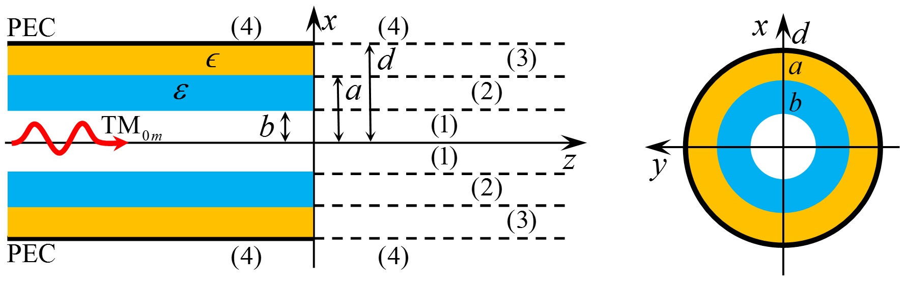
Figure 1: Geometry of the problem and main notations.

$$H_{\omega\varphi}^{(i)}=M^{(i)}e^{ik_{zl}z}\left\{\begin{aligned} &\left.J_{1}(\rho\sigma_{l})\right/\sigma_{l}\quad\text{for }\rho<b,\\ &\frac{J_{1}(b\sigma_{l})}{\sigma_{l}}\frac{\psi_{l}(\rho)}{\psi_{l}(b)}\,\,\,\text{for }b<\rho<a,\\ &\frac{J_{1}(b\sigma_{l})}{\sigma_{l}}\frac{\psi_{l}(a)}{\psi_{l}(b)}\frac{\psi_{0l}(\rho)}{\psi_{0l}(a)}\,\,\,\,\text{for }a<\rho<d,\end{aligned}\right.$$ (3)

where $M^{(i)}$ is an arbitrary amplitude constant,

$$\psi_{0m}(\xi) =J_{1}(\xi\chi_{m})Y_{0}(d\chi_{m})-N_{1}(\xi\chi_{m})J_{0}(d\chi_{m}),$$ (4)

$$\psi_{m}(\xi) =J_{1}(\xi s_{m})\varphi_{2m}-N_{1}(\xi s_{m})\varphi_{1m},$$

$$\varphi_{1m} =\sigma_{m}J_{0}(b\sigma_{m})J_{1}(bs_{m})-s_{m}\varepsilon^{-1}J_{1}(b\sigma_{m})J_{0}(bs_{m}),$$

$$\varphi_{2m} =\sigma_{m}J_{0}(b\sigma_{m})Y_{1}(bs_{m})-s_{m}\varepsilon^{-1}J_{1}(b\sigma_{m})Y_{0}(bs_{m}),$$

$J_{\nu}$ and $Y_{\nu}$ are Bessel and Neumann functions of $\nu$-th order, correspondingly, transverse wave numbers $\sigma_{m}$, $s_{m}$ and $\chi_{m}$ are determined by the following dispersion equation

$$\mathrm{det}\hat{M}=0,$$ (5)

$$\hat{M}{=}\left(\begin{array}[]{cccc}\varphi_{1m}&\varphi_{2m}&0&0\\ J_{1}(as_{m})&Y_{1}(as_{m})&-J_{1}(a\chi_{m})&-Y_{1}(a\chi_{m})\\ \frac{s_{m}J_{0}(as_{m})}{\varepsilon}&\frac{s_{m}Y_{0}(as_{m})}{\varepsilon}&\frac{-\chi_{m}J_{0}(a\chi_{m})}{\epsilon}&\frac{-\chi_{m}Y_{0}(a\chi_{m})}{\epsilon}\\ 0&0&J_{0}(d\chi_{m})&Y_{0}(d\chi_{m})\end{array}\right),$$ (6)

longitudinal wave number $k_{z}$ is connected with $\sigma_{m}$, $s_{m}$ and $\chi_{m}$ as follows:

$$k_{zm} =\sqrt{k_{0}^{2}-\sigma_{m}^{2}}=\sqrt{k_{0}^{2}\varepsilon-s_{m}^{2}}=$$ (7)

$$=\sqrt{k_{0}^{2}\epsilon-\chi_{m}^{2}},\quad\mathrm{Im}k_{zm}>0,$$

$k_{0}=\omega/c+i\delta$ ($\delta\to 0$, which is equivalent to infinitely small dissipation an all areas), $c$ is the light speed in vacuum. From (7) one can express both $s_{m}$ and $\chi_{m}$ through $\sigma_{m}$ and obtain the dispersion relation with respect to a single variable $\sigma_{m}$. Note that Eq. (3) transforms to the corresponding mode of a two-layer waveguide Galyamin and Vorobev (2022) for $\epsilon\to\varepsilon$.

The reflected field in the area inside the waveguide ($z<0$, $\rho<a$) is decomposed into a series of TM modes propagating in the opposite direction:

$$H_{\omega\varphi}^{(r)}=\sum\limits_{m=0}^{\infty}M_{m}e^{-ik_{zm}z}\left\{\begin{aligned} &\left.J_{1}(\rho\sigma_{m})\right/\sigma_{m}\quad\text{for }\rho<b,\\ &\frac{J_{1}(b\sigma_{m})}{\sigma_{m}}\frac{\psi_{m}(\rho)}{\psi_{m}(b)}\,\,\,\text{for }b<\rho<a,\\ &\frac{J_{1}(b\sigma_{m})}{\sigma_{m}}\frac{\psi_{m}(a)}{\psi_{m}(b)}\frac{\psi_{0m}(\rho)}{\psi_{0m}(a)}\\ &\quad\quad\quad\quad\quad\text{for }a<\rho<d,\end{aligned}\right.$$ (8)

where $\{M_{m}\}$ are unknown “reflection coefficients” that should be determined. Note that since both the structure and the excitation (3) are uniform in $\varphi$ then only symmetric TM modes are taken into account in the reflected field.

The area outside the waveguide is divided into three subareas “1”, “2”, “3” and “4” (see Fig. 1), where the field is described by Helmholtz equation:

$$\left[\frac{\partial^{2}}{\partial z^{2}}+\frac{\partial^{2}}{\partial\rho^{2}}+\frac{1}{\rho}\frac{\partial}{\partial\rho}+\left(k_{0}^{2}-\frac{1}{\rho^{2}}\right)\right]H_{\omega\varphi}^{(1,2,3,4)}=0.$$ (9)

We introduce functions ${{\Psi}_{\pm}}(\rho,\alpha)$ (hereafter subscripts $\pm$ mean that function is holomorphic and free of poles and zeros in areas $\operatorname{Im}\alpha>-\delta$ and $\operatorname{Im}\alpha<\delta$, correspondingly):

$$\Psi_{+}^{(1,2,3,4)}(\rho,\alpha)={{(2\pi)}^{-1}}\int_{0}^{\infty}{dzH_{\omega\varphi}^{(1,2,3,4)}(\rho,z){{e}^{i\alpha z}}},$$ (10)

$$\Psi_{-}^{(4)}(\rho,\alpha)={{(2\pi)}^{-1}}\int_{-\infty}^{0}{dzH_{\omega\varphi}^{(4)}(\rho,z){{e}^{i\alpha z}}},$$ (11)

and similar transforms of $E_{\omega z}^{(1,2,3,4)}$, for example,

$$\Phi_{+}^{(1,2,3,4)}(\rho,\alpha)={{(2\pi)}^{-1}}\int_{0}^{\infty}{dz\frac{k_{0}}{i}E_{\omega z}^{(1,2,3,4)}(\rho,z){{e}^{i\alpha z}}}.$$ (12)

From (12) and (2) we have the following relation between $\Phi$ and $\Psi$:

$$\Phi_{+}^{(1,2,3,4)}(\rho,\alpha)=\frac{\Psi_{+}^{(1,2,3,4)}(\rho,\alpha)}{\rho}+\frac{\partial\Psi_{+}^{(1,2,3,4)}(\rho,\alpha)}{\partial\rho},$$ (13)

and the same relation between $\Phi_{-}^{(4)}(\rho,\alpha)$ and $\Psi_{-}^{(4)}(\rho,\alpha)$.

From (9) we obtain

$$\left(\frac{{{\partial}^{2}}}{\partial{{\rho}^{2}}}{+}\frac{1}{\rho}\frac{\partial}{\partial\rho}{+}{{\kappa}^{2}}{-}\frac{1}{\rho^{2}}\right)\left\{\begin{matrix}\Psi_{+}^{(1,2,3)}\\ \Psi_{-}^{(4)}{+}\Psi_{+}^{(4)}\\ \end{matrix}\right\}{=}\left\{\begin{matrix}{{F}^{(1,2,3)}}\\ 0\\ \end{matrix}\right\},$$ (14)

$$2\pi F^{(1,2,3)}={\left.{\partial H_{\omega\varphi}^{(1,2,3)}}/{\partial z}\right|}_{z=0_{+}}-{\left.i\alpha H_{\omega\varphi}^{(1,2,3)}\right|}_{z=0_{+}},$$ (15)

where

$$\kappa=\sqrt{k_{0}^{2}-{{\alpha}^{2}}},\quad\operatorname{Im}\kappa>0.$$ (16)

Equation (14) is obtained in a similar way as Eq. (9) in Galyamin et al. (2021).

Functions ${{F}^{(1,2,3)}}$ are determined using continuity of $E_{\omega\rho}$ and $H_{\omega\varphi}$ for $z=0$, $\rho<d$ (see Galyamin et al. (2021) for details), therefore

$$2\pi{{F}^{(1)}} =i\left[\vphantom{\sum\nolimits_{m=1}^{\infty}}\left(k_{zl}-\alpha\right)M^{(i)}\left.J_{1}(\rho\sigma_{l})\right/\sigma_{l}\right.$$ (17)

$$\left.-\sum\nolimits_{m=1}^{\infty}\left(k_{zm}+\alpha\right)M_{m}\left.J_{1}(\rho\sigma_{m})\right/\sigma_{m}\right],$$

$$2\pi F^{(2)} =i\left[M^{(i)}\left(\frac{k_{zl}}{\varepsilon}-\alpha\right)\frac{J_{1}(b\sigma_{l})}{\sigma_{l}}\frac{\psi_{l}(\rho)}{\psi_{l}(b)}\right.$$ (18)

$$-\sum\limits_{m=1}^{\infty}M_{m}\left(\frac{k_{zm}}{\varepsilon}+\alpha\right)\frac{J_{1}(b\sigma_{m})}{\sigma_{m}}\frac{\psi_{m}(\rho)}{\psi_{m}(b)}\left.\vphantom{\left(\frac{k_{zl}}{\varepsilon}-\alpha\right)}\right],$$

$$2\pi F^{(3)} =i\left[M^{(i)}\left(\frac{k_{zl}}{\epsilon}-\alpha\right)\frac{J_{1}(b\sigma_{l})}{\sigma_{l}}\frac{\psi_{l}(a)}{\psi_{l}(b)}\frac{\psi_{0l}(\rho)}{\psi_{0l}(a)}\right.$$ (19)

$$-\sum\limits_{m=1}^{\infty}M_{m}\left(\frac{k_{zm}}{\epsilon}+\alpha\right)\frac{J_{1}(b\sigma_{m})}{\sigma_{m}}\frac{\psi_{m}(a)}{\psi_{m}(b)}\frac{\psi_{0m}(\rho)}{\psi_{0m}(a)}\left.\vphantom{\left(\frac{k_{zl}}{\varepsilon}-\alpha\right)}\right].$$

General solution of Eq. (14) has the form (see Galyamin et al. (2021) for details):

$$\Psi_{+}^{(1)}(\rho,\alpha) =C^{(1)}J_{1}(\rho\kappa)+\Psi_{p}^{(1)}(\rho,\alpha),$$ (20)

$$\Psi_{+}^{(2)}(\rho,\alpha) =C^{(2)}_{1}J_{1}(\rho\kappa)$$

$$+C^{(2)}_{2}Y_{1}(\rho\kappa)+\Psi_{p}^{(2)}(\rho,\alpha),$$ (21)

$$\Psi_{+}^{(3)}(\rho,\alpha) =C^{(3)}_{1}J_{1}(\rho\kappa)$$

$$+C^{(3)}_{2}Y_{1}(\rho\kappa)+\Psi_{p}^{(3)}(\rho,\alpha),$$ (22)

$$\Psi_{-}^{(4)}(\rho,\alpha) +\Psi_{+}^{(4)}(\rho,\alpha)=C^{(4)}H_{1}^{(1)}(\rho\kappa),$$ (23)

where $H^{(1)}_{\nu}$ is a Hankel function of the first kind of $\nu$-th order, $C^{(1,4)}$ and $C^{(2,3)}_{1,2}$ are unknown coefficients.

Particular solutions of the inhomogeneous equations $\Psi_{p}^{(1,2,3)}$ have the form (see Galyamin et al. (2021) for details)

$$\Psi_{p}^{(1)}(\rho,\alpha)=\frac{iM^{(i)}}{2\pi\sigma_{l}}\frac{J_{1}\left(\rho\sigma_{l}\right)}{k_{zl}+\alpha}-\sum\limits_{m=1}^{\infty}\frac{iM_{m}}{2\pi\sigma_{m}}\frac{J_{1}\left(\rho\sigma_{m}\right)}{k_{zm}-\alpha},$$ (24)

$$\Psi_{p}^{(2)}(\rho,\alpha)=\frac{iM^{(i)}}{2\pi}\frac{\frac{k_{zl}}{\varepsilon}-\alpha}{\kappa^{2}-s_{l}^{2}}\frac{J_{1}(b\sigma_{l})}{\sigma_{l}}\frac{\psi_{l}(\rho)}{\psi_{l}(b)}$$ (25)

$$-\sum\limits_{m=1}^{\infty}\frac{iM_{m}}{2\pi}\frac{\frac{k_{zm}}{\varepsilon}+\alpha}{\kappa^{2}-s_{m}^{2}}\frac{J_{1}(b\sigma_{m})}{\sigma_{m}}\frac{\psi_{m}(\rho)}{\psi_{m}(b)},$$

$$\Psi_{p}^{(3)}(\rho,\alpha)=\frac{iM^{(i)}}{2\pi}\frac{\frac{k_{zl}}{\epsilon}-\alpha}{\kappa^{2}-\chi_{l}^{2}}\frac{J_{1}(b\sigma_{l})}{\sigma_{l}}\frac{\psi_{l}(a)}{\psi_{l}(b)}\frac{\psi_{0l}(\rho)}{\psi_{0l}(a)}$$ (26)

$$-\sum\limits_{m=1}^{\infty}\frac{iM_{m}}{2\pi}\frac{\frac{k_{zm}}{\epsilon}+\alpha}{\kappa^{2}-\chi_{m}^{2}}\frac{J_{1}(b\sigma_{m})}{\sigma_{m}}\frac{\psi_{m}(a)}{\psi_{m}(b)}\frac{\psi_{0m}(\rho)}{\psi_{0m}(a)}.$$

From Eq. (13) one obtains corresponding form of general solution for $\Phi$:

$$\Phi_{+}^{(1)}(\rho,\alpha) =ik_{0}^{-1}C^{(1)}\kappa J_{0}(\rho\kappa)+\Phi_{p}^{(1)}(\rho,\alpha),$$ (27)

$$\Phi_{+}^{(2)}(\rho,\alpha) =ik_{0}^{-1}C^{(2)}_{1}\kappa J_{0}(\rho\kappa)$$

$$+ik_{0}^{-1}C^{(2)}_{2}\kappa J_{0}(\rho\kappa)+\Phi_{p}^{(2)}(\rho,\alpha),$$ (28)

$$\Phi_{+}^{(3)}(\rho,\alpha) =ik_{0}^{-1}C^{(3)}_{1}\kappa J_{0}(\rho\kappa)$$

$$+ik_{0}^{-1}C^{(3)}_{2}\kappa J_{0}(\rho\kappa)+\Phi_{p}^{(3)}(\rho,\alpha),$$ (29)

$$\Phi_{-}^{(4)}(\rho,\alpha) +\Phi_{+}^{(4)}(\rho,\alpha)=ik_{0}^{-1}C^{(4)}\kappa H_{0}^{(1)}(\rho\kappa),$$ (30)

where

$$\Phi_{p}^{(1)}(\rho,\alpha)=\frac{-M^{(i)}}{2\pi k_{0}}\frac{J_{0}(\rho\sigma_{l})}{k_{zl}+\alpha}+\sum\limits_{m=1}^{\infty}\frac{M_{m}}{2\pi k_{0}}\frac{J_{0}\left(\rho\sigma_{m}\right)}{k_{zm}-\alpha},$$ (31)

$$\Phi_{p}^{(2)}(\rho,\alpha)=\frac{-M^{(i)}}{2\pi k_{0}}\frac{\frac{k_{zl}}{\varepsilon}-\alpha}{\kappa^{2}-s_{l}^{2}}\frac{s_{l}J_{1}(b\sigma_{l})}{\sigma_{l}}\frac{\phi_{l}(\rho)}{\phi_{l}(b)}$$ (32)

$$+\sum\limits_{m=1}^{\infty}\frac{M_{m}}{2\pi k_{0}}\frac{\frac{k_{zm}}{\varepsilon}+\alpha}{\kappa^{2}-s_{m}^{2}}\frac{s_{m}J_{1}(b\sigma_{m})}{\sigma_{m}}\frac{\phi_{m}(\rho)}{\phi_{m}(b)},$$

$$\Phi_{p}^{(3)}(\rho,\alpha)=\frac{-M^{(i)}}{2\pi k_{0}}\frac{\frac{k_{zl}}{\epsilon}-\alpha}{\kappa^{2}-\chi_{l}^{2}}\frac{J_{1}(b\sigma_{l})}{\sigma_{l}}\frac{\psi_{l}(a)}{\psi_{l}(b)}\frac{\chi_{l}\phi_{0l}(\rho)}{\phi_{0l}(a)}$$ (33)

$$+\sum\limits_{m=1}^{\infty}\frac{M_{m}}{2\pi k_{0}}\frac{\frac{k_{zm}}{\varepsilon}+\alpha}{\kappa^{2}-\chi_{m}^{2}}\frac{J_{1}(b\sigma_{m})}{\sigma_{m}}\frac{\psi_{m}(a)}{\psi_{m}(b)}\frac{\chi_{m}\phi_{0m}(\rho)}{\phi_{0m}(a)},$$

where

$$\phi_{0m}(\rho) =J_{0}(\rho\chi_{m})Y_{0}(d\chi_{m})-N_{0}(\rho\chi_{m})J_{0}(d\chi_{m}),$$ (34)

$$\phi_{m}(\rho) =J_{0}(\rho s_{m})\varphi_{2m}-N_{0}(\rho s_{m})\varphi_{1m},$$

and $\Phi_{p}^{(3)}(d,\alpha)=0$ since $\phi_{0m}(d)=0$.

Boundary condition $E_{\omega z}=0$ for $\rho=d$, $z<0$ results in $\Phi_{-}^{(4)}(d,\alpha)=0$, and we obtain from (30):

$$C^{(4)}=\frac{k_{0}\Phi_{+}^{(4)}(d,\alpha)}{i\kappa H_{1}^{(1)}(d\kappa)},$$ (35)

therefore from Eq. (23)

$$\Psi_{+}^{(4)}(d,\alpha)+\Psi_{-}^{(4)}(d,\alpha)=\frac{k_{0}\Phi_{+}^{(4)}(a,\alpha)H_{1}^{(1)}(d\kappa)}{i\kappa H_{1}^{(1)}(d\kappa)}.$$ (36)

To obtain Wiener-Hopf-Fock equation one should express the term $\Psi_{+}^{(4)}(d,\alpha)$ in Eq. (36) through the $\Phi_{+}^{(4)}(d,\alpha)$. This can be done using the continuity conditions for $\rho=b,a,d$, $z>0$ (see Galyamin and Vorobev (2022) for details):

$$\Psi_{+}^{(4)}(d,\alpha) =\frac{k_{0}\Phi_{+}^{(4)}(d,\alpha)J_{1}(d\kappa)}{i\kappa J_{0}(d\kappa)}+\Psi_{p}^{(3)}(d,\alpha)$$ (37)

$$-\frac{k_{0}}{i\kappa dJ_{0}(d\kappa)} \left[bJ_{1}(b\kappa)\left(\Phi_{p}^{(1)}(b,\alpha)-\Phi_{p}^{(2)}(b,\alpha)\right)\right.$$

$$+aJ_{1}(a\kappa)\left(\Phi_{p}^{(2)}(a,\alpha)-\Phi_{p}^{(1)}(a,\alpha)\right)$$

$$-\frac{ib\kappa J_{0}(b\kappa)}{k_{0}}\left(\Psi_{p}^{(1)}(b,\alpha)-\Psi_{p}^{(2)}(b,\alpha)\right)$$

$$-\left.\frac{ia\kappa J_{0}(a\kappa)}{k_{0}}\left(\Psi_{p}^{(2)}(a,\alpha)-\Psi_{p}^{(3)}(a,\alpha)\right)\right].$$

Similar to Galyamin et al. (2021); Galyamin and Vorobev (2022), the right-hand side of (37) formally possesses pole singularity for $\alpha=\alpha_{m}$:

$$\alpha_{m}=\sqrt{k_{0}^{2}-j_{0m}^{2}d^{-2}},\quad\mathrm{Im}\alpha_{m}>0,$$ (38)

where $j_{0m}$ is the $m$-th zero of Bessel function $J_{0}$ ($\alpha_{m}$ are longitudinal wavenumbers of vacuum waveguide of radius $d$). However, the function determined by Eq. (37) should be regular in the area $\mathrm{Im}\alpha>-\delta$. Therefore, this pole singularity at the right-hand side should be eliminated and we obtain the following requirement:

$$\Phi_{+}^{(4)}(d,\alpha_{p})J_{1}(j_{0p})=\frac{1}{d}\left\{\vphantom{\left[\Phi_{p}^{(1)}(b,\alpha_{p})-\Phi_{p}^{(2)}(b,\alpha_{p})\right]}bJ_{1}(bj_{0p}/d)\right.$$ (39)

$$\times\left[\Phi_{p}^{(1)}(b,\alpha_{p})-\Phi_{p}^{(2)}(b,\alpha_{p})\right]$$ (40)

$$+aJ_{1}(aj_{0p}/d)\left[\Phi_{p}^{(2)}(a,\alpha_{p})-\Phi_{p}^{(1)}(a,\alpha_{p})\right]$$ (41)

$$-\frac{ibj_{0p}J_{0}(bj_{0p}/d)}{dk_{0}}\left[\Psi_{p}^{(1)}(b,\alpha_{p})-\Psi_{p}^{(2)}(b,\alpha_{p})\right]$$ (42)

$$-\left.\frac{iaj_{0p}J_{0}(aj_{0p}/d)}{dk_{0}}\left[\Psi_{p}^{(2)}(a,\alpha_{p})-\Psi_{p}^{(3)}(a,\alpha_{p})\right]\right\}.$$ (43)

Substituting Eq. (37) into Eq. (36) and combining the terms proportional to $\Phi_{+}^{(4)}(d,\alpha)$ we obtain the following Wiener-Hopf-Fock equation:

$$\frac{2k_{0}\Phi_{+}^{(4)}(d,\alpha)}{\kappa G(\alpha)}+\Psi_{-}^{(4)}(d,\alpha)+\frac{1}{dJ_{0}(d\kappa)}\frac{i}{2\pi}\Pi(\alpha)=0,$$ (44)

where

$$G(\alpha)=\pi a\kappa J_{0}(a\kappa)H_{0}^{(1)}(a\kappa),$$ (45)

$$\Pi(\alpha)=b\frac{M^{(i)}\zeta_{1l}(\alpha)}{k_{zl}+\alpha}-\sum\limits_{m=0}^{infty}b\frac{M_{m}\zeta_{1m}(\alpha)}{k_{zm}-\alpha}$$ (46)

$$+M^{(i)}\frac{\frac{k_{zl}}{\varepsilon}-\alpha}{\kappa^{2}-s_{l}^{2}}\frac{s_{l}J_{1}(b\sigma_{l})}{\sigma_{l}\psi_{l}(b)}\eta_{1l}(\alpha)$$

$$-\sum\limits_{m=0}^{\infty}M_{m}\frac{\frac{k_{zm}}{\varepsilon}+\alpha}{\kappa^{2}-s_{m}^{2}}\frac{s_{m}J_{1}(b\sigma_{m})}{\sigma_{m}\psi_{m}(b)}\eta_{1m}(\alpha)$$

$$+aM^{(i)}\frac{\frac{k_{zl}}{\epsilon}-\alpha}{\kappa^{2}-\chi_{l}^{2}}\frac{J_{1}(b\sigma_{l})}{\sigma_{l}}\frac{\psi_{l}(a)}{\psi_{l}(b)\psi_{0l}(a)}\eta_{2l}(\alpha)$$

$$-\sum\limits_{m=0}^{\infty}aM_{m}^{(i)}\frac{\frac{k_{zm}}{\epsilon}+\alpha}{\kappa^{2}-\chi_{m}^{2}}\frac{J_{1}(b\sigma_{m})}{\sigma_{m}}\frac{\psi_{m}(a)}{\psi_{m}(b)\psi_{0m}(a)}\eta_{2m}(\alpha),$$

$$\eta_{1m}(\alpha)=b\phi_{2m}\mu_{bm}(\alpha)-a\phi_{2m}\mu_{am}(\alpha)$$ (47)

$$-b\phi_{1m}\nu_{bm}(\alpha)+a\phi_{1m}\nu_{am}(\alpha),$$

$$\mu_{bm}(\alpha)=J_{0}(b\kappa)J_{1}(bs_{m})/s_{m}-J_{0}(bs_{m})J_{1}(b\kappa)/\kappa,$$

$$\nu_{bm}(\alpha)=J_{0}(b\kappa)Y_{1}(bs_{m})/s_{m}-Y_{0}(bs_{m})J_{1}(b\kappa)/\kappa,$$

$$\mu_{am}(\alpha)=J_{0}(a\kappa)J_{1}(as_{m})/s_{m}-J_{0}(as_{m})J_{1}(a\kappa)/\kappa,$$

$$\nu_{am}(\alpha)=J_{0}(a\kappa)Y_{1}(as_{m})/s_{m}-Y_{0}(as_{m})J_{1}(a\kappa)/\kappa,$$

$$\eta_{2m}(\alpha)=\chi_{m}Y_{0}(d\chi_{m})\zeta_{2m}$$

$$+J_{0}(d\chi_{m})\left(\chi_{m}J_{1}(a\kappa)Y_{0}(a\chi_{m})/\kappa-J_{0}(a\kappa)Y_{1}(a\chi_{m})\right)$$

$$-2J_{0}(d\kappa)(\pi a\chi_{m})^{-1},$$

$$\zeta_{1m}(\alpha)=J_{0}(b\sigma_{m})J_{1}(b\kappa)/\kappa-J_{0}(b\kappa)J_{1}(b\sigma_{m})/\sigma_{m}.$$

Equation (44) is solved in a common way (see Mittra and Lee (1971); Galyamin et al. (2021); Galyamin and Vorobev (2022) for details). Omitting standard factorizations and estimations, we obtain:

$$\Phi_{+}^{(4)}(d,\alpha)=\frac{1}{4\pi ik_{0}d}\kappa_{+}(\alpha)G_{+}(\alpha)$$ (48)

$$\times\sum\limits_{q=1}^{\infty}\Pi(-\alpha_{q})\frac{\kappa_{+}(\alpha_{q})G_{+}(\alpha_{q})j_{0q}}{d^{2}\alpha_{q}J_{1}(j_{0q})(\alpha+\alpha_{q})}.$$

To find $\{M_{m}\}$, one should substitute (48) into (39). After transformations we obtain an infinite linear system of the form

$$\sum\nolimits_{m=1}^{\infty}W_{pm}M_{m}=M^{(i)}w_{p},\quad p=1,2,\ldots,$$ (49)

which is convergent and can be solved numerically using the reducing technique (see, for example, Galyamin et al. (2021); Galyamin and Vorobev (2022) for details).

III EM field derivation

When the set of coefficients $\{M_{m}\}$ is determined, the electromagnetic field can be calculated via the inverse transform over $\alpha$, in accordance with Eqs. (10) and (11):

$$H_{\omega\varphi}^{(1,2,3)}(\rho,z>0) =\int\nolimits_{-\infty}^{+\infty}\Psi^{(1,2,3)}_{+}(\rho,\alpha)e^{-i\alpha z}\,d\alpha,$$ (50)

$$H_{\omega\varphi}^{(4)}(\rho,z) =\int\nolimits_{-\infty}^{+\infty}\Psi^{(4)}(\rho,\alpha)e^{-i\alpha z}\,d\alpha.$$ (51)

performing calculations similar to those done in Galyamin and Vorobev (2022), one obtains that the field in the region $z>0$ is described by the unified formula:

$$H_{\omega\varphi}^{(1,2,3)}(\rho,z>0)=\sum\limits_{q=1}^{\infty}\Pi(-\alpha_{q})\frac{\kappa_{+}(\alpha_{q})G_{+}(\alpha_{q})j_{0q}}{d^{2}\alpha_{q}J_{1}(j_{0q})}\frac{L_{q}^{+}(\rho,z)}{2},$$ (52)

where $L_{q}^{+}$ is given by Eq. (47) in Galyamin et al. (2021).

For the domain “4” one can also obtain the representation convenient for investigation of the far-field:

$$H_{\omega\varphi}^{(4)}(\rho,z)=\frac{1}{d}\sum\limits_{q=1}^{\infty}\Pi(-\alpha_{q})\frac{\kappa_{+}(\alpha_{q})G_{+}(\alpha_{q})j_{0q}}{d^{2}\alpha_{q}J_{1}(j_{0q})}\frac{I_{q}^{(4)}}{4\pi},$$ (53)

where integral

$$I_{q}^{(4)}(\rho,z)=\int\limits_{-\infty}^{+\infty}\!\!\frac{\kappa_{+}(\alpha)G_{+}(\alpha)H_{1}^{(1)}(\rho\kappa)}{\kappa(\alpha)H_{0}^{(1)}(a\kappa)(\alpha_{q}+\alpha)}e^{-i\alpha z}\,d\alpha$$ (54)

has been investigated previously (see Eq. (41) in Galyamin et al. (2021)). In particular, integral (54) can be easily calculated asymptotically (see Eq. (51) in Galyamin et al. (2021)) and substituted into (53) to obtain far-field in the region “4”.

IV Conclusion

We have presented convenient rigorous analytical approach for calculation of various diffraction processes at the open end (with orthogonal cut) of a circular waveguide with three-layer dielectric lining. This approach can be effectively used for investigation of radiation of Cherenkov wakefield from the open-ended capillary (see Ref. Jiang et al. (2020)) which is a promising structure for realization of beam-driven THz source with small divergence and high efficiency. Moreover, this approach can be extended to more complicated problems. For example, excitation by a charged particle bunch (in full formulation including both wakefield radiation and transition radiation) can be incorporated into the solution.

V Acknowledgements

Author is grateful to A.M. Altmark for fruitful discussions. This work is supported by the Russian Science Foundation (grant No. 18-72-10137).