GOCPT: Generalized Online Canonical Polyadic Tensor Factorization
and Completion

Abstract

Low-rank tensor factorization or completion is well-studied and applied in various online settings, such as online tensor factorization (where the temporal mode grows) and online tensor completion (where incomplete slices arrive gradually). However, in many real-world settings, tensors may have more complex evolving patterns: (i) one or more modes can grow; (ii) missing entries may be filled; (iii) existing tensor elements can change. Existing methods cannot support such complex scenarios. To fill the gap, this paper proposes a Generalized Online Canonical Polyadic (CP) Tensor factorization and completion framework (named GOCPT) for this general setting, where we maintain the CP structure of such dynamic tensors during the evolution. We show that existing online tensor factorization and completion setups can be unified under the GOCPT framework. Furthermore, we propose a variant, named $\mbox{{GOCPT}}_{\mathrm{E}}$, to deal with cases where historical tensor elements are unavailable (e.g., privacy protection), which achieves similar fitness as GOCPT but with much less computational cost. Experimental results demonstrate that our GOCPT can improve fitness by up to $2.8\%$ on the JHU Covid data and $9.2\%$ on a proprietary patient claim dataset over baselines. Our variant $\mbox{{GOCPT}}_{\mathrm{E}}$ shows up to $1.2\%$ and $5.5\%$ fitness improvement on two datasets with about $20\%$ speedup compared to the best model.

1 Introduction

Streaming tensor data becomes increasingly popular in areas such as spatio-temporal outlier detection Najafi et al. (2019), social media Song et al. (2017), sensor monitoring Mardani et al. (2015), video analysis Kasai (2019) and hyper-order time series Cai et al. (2015). The factorization/decomposition of such multidimensional structural data is challenging since they are usually sparse, delayed, and sometimes incomplete. There is an increasing need to maintain the low-rank Tucker Sun et al. (2006); Xiao et al. (2018); Nimishakavi et al. (2018); Fang et al. (2021); Gilman and Balzano (2020) or CP Du et al. (2018); Phipps et al. (2021) structure of the evolving tensors in such dynamics, considering model efficiency and scalability.

Several online (we also use “streaming” interchangeably) settings have been discussed before. The most popular two are online tensor decomposition Zhou et al. (2016); Song et al. (2017) and online tensor completion Kasai (2019), where the temporal mode grows with new incoming slices. Some pioneer works have been proposed for these two particular settings. For the factorization problem, Nion and Sidiropoulos (2009) incrementally tracked the singular value decomposition (SVD) of the unfolded third-order tensors to maintain the CP factorization results. Accelerated methods have been proposed for the evolving dense Zhou et al. (2016) or sparse Zhou et al. (2018) tensors by reusing intermediate quantities, e.g., matricized tensor times Khatri-Rao product (MTTKRP). For the completion problem, recursive least squares Kasai (2016) and stochastic gradient descent (SGD) Mardani et al. (2015) were studied to track the evolving subspace of incomplete data.

However, most existing methods are designed for the growing patterns. They cannot support other possible patterns (e.g., missing entries in the previous tensor can be refilled or existing values can be updated) or more complex scenarios where the tensors evolve with a combination of patterns.

Motivating application: Let us consider a public health surveillance application where data is modeled as a fourth-order tensor indexed by location (e.g., zip code), disease (e.g., diagnosis code), data generation date (GD) (i.e., the date when the clinical events actually occur) and data loading date (LD) (i.e., the time when the events are reported in the database) and each tensor element stands for the count of medical claims with particular location-disease-date tuples. The tensor grows over time by adding new locations, diseases, GD’s, or LD’s. For every new LD, missing entries before that date may be filled in, and existing entries can be revised for data correction purposes Qian et al. (2021). Dealing with such a dynamic tensor is challenging, and very few works have studied this online tensor factorization/completion problem. The most recent work in Qian et al. (2021) can only handle a special case with the GD dimension growing but not with data correction or two more dimensions growing simultaneously.

To fill the gap, we propose GOCPT – a general framework that deals with the above-mentioned online tensor updating scenarios. The major contributions of the paper are summarized as follows:

• We propose a unified framework GOCPT for online tensor factorization/completion with complex evolving patterns such as mode growth, missing filling, and value update, while previous models cannot handle such general settings.

• We propose $\mbox{{GOCPT}}_{\mathrm{E}}$, i.e., a more memory and computational efficient version of GOCPT, to deal with cases where historical tensor elements are unavailable due to limited storage or privacy-related issues.

• We experimentally show that both GOCPT and $\mbox{{GOCPT}}_{\mathrm{E}}$ work well under a combination of online tensor challenges. The GOCPT improves the fitness by up to $2.8\%$ and $9.2\%$ on real-world Covid and medical claim datasets, respectively. In comparison, $\mbox{{GOCPT}}_{\mathrm{E}}$ provides comparable fitness scores as GOCPT with $20\%+$ complexity reduction compared to the baseline methods.

The first version of GOCPT package has been released in PyPI and open-sourced in GitHub. Supplementary of this paper can be found in the same GitHub repository.

2 Problem Formulation

Notations.

We use plain letters for scalars, e.g., $x$ or $X$, boldface uppercase letters for matrices, e.g., $\mathbf{X}$, boldface lowercase letters for vectors, e.g., $\mathbf{x}$, and Euler script letters for tensors or sets, e.g., $\mathcal{X}$. Tensors are multidimensional arrays indexed by three or more modes. For example, an $N_{th}$-order tensor $\mathcal{X}$ is an $N$-dimensional array of size $I_{1}\times I_{2}\times\cdots\times I_{N}$, where $x_{i_{1}i_{2}\cdots i_{N}}$ is the element at the $(i_{1},i_{2},\cdots,i_{N})$ location. For a matrix $\mathbf{X}$, the $r$-th row is denoted by $\mathbf{x}_{r}$. We use $\stackMath\mathbin{\stackinset{c}{0ex}{c}{0ex}{\ast}{\ocircle}}$ for Hadamard product (element-wise product), $\odot$ for Khatri-Rao product, and $\llbracket\cdot\rrbracket$ for Kruskal product (which inputs matrices and outputs a tensor).

For an incomplete observation of tensor $\mathcal{X}$, we use a mask tensor $\Omega$ to indicate the observed entries: if $x_{i_{1}i_{2}\cdots i_{N}}$ is observed, then $\Omega_{i_{1}i_{2}\cdots i_{N}}=1$, otherwise $0$. Thus, $\mathcal{X}\stackMath\mathbin{\stackinset{c}{0ex}{c}{0ex}{\ast}{\ocircle}}\Omega$ is the actual observed data. In this paper, $\Omega$ can also be viewed as an index set of the observed entries. We define $\|(\cdot)_{\Omega}\|_{F}^{2}$ as the sum of element-wise squares restricted on $\Omega$, e.g.,

$$\left\|(\mathcal{X}-\mathcal{Y})_{\Omega}\right\|_{F}^{2}\equiv\sum_{(i_{1},\cdots,i_{N})\in\Omega}(x_{i_{1}\cdots i_{N}}-y_{i_{1}\cdots i_{N}})^{2},$$

where $\mathcal{X}$ and $\mathcal{Y}$ may not necessarily be of the same size, but $\Omega$ must index within the bounds of both tensors. We describe basic matrix/tensor algebra in appendix A, where we also list a table to summarize all the notations used in the paper.

2.1 Problem Definition

Modeling Streaming Tensors.

Real-world streaming data comes with indexing features and quantities, for example, we may receive a set of disease count tuples on a daily basis, e.g., (location, disease, date; count), where the first three features can be used to locate in a third-order tensor and the counts can be viewed as tensor elements.

Formally, a streaming of index-element tuples, e.g., represented by $(i_{1},\cdots,i_{N};~{}x_{i_{1}\cdots i_{N}})$, can be modeled as an evolving tensor structure. This paper considers three typical types of evolution, shown in Fig. 1.

• (i) Mode growth. New (incomplete) slices are added along one or more modes. Refer to the blue parts.

• (ii) Missing filling. Some missing values in the old tensor is received. Refer to the green entries in the figure.

• (iii) Value update. Previously observed entries may change due to new information. Refer to yellow entries.

To track the evolution process, this paper proposes a general framework for solving the following problem on the fly.

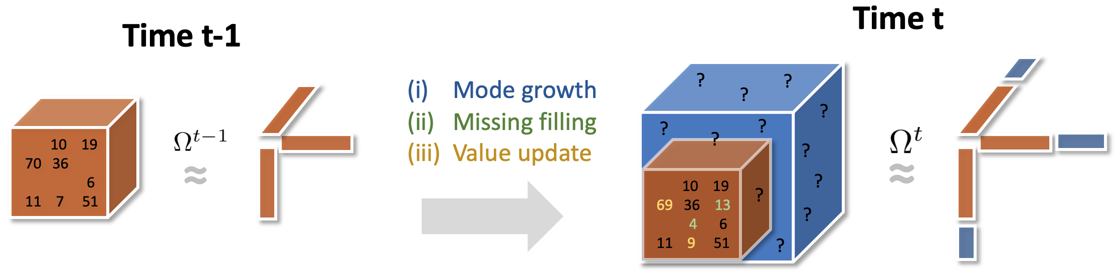
Figure 1: Illustration of Online Tensor Evolution

Problem 1 (Online Tensor Factorization and Completion).

Suppose tensor $\mathcal{X}^{t-1}\in\mathbb{R}^{I_{1}^{t-1}\times\cdots\times I_{N}^{t-1}}$ admits a low-rank approximation $\mathcal{Y}^{t-1}$ at time $(t-1)$, parametrized by rank-$R$ factors $\{\mathbf{A}^{n,t-1}\in\mathbb{R}^{I_{n}^{t-1}\times R}\}_{n=1}^{N}$, i.e., $\mathcal{Y}^{t-1}=\llbracket\mathbf{A}^{1,t-1},\cdots,\mathbf{A}^{N,t-1}\rrbracket$. Given the mask $\Omega^{t-1}$, it satisfies

$$\Omega^{t-1}\stackMath\mathbin{\stackinset{c}{0ex}{c}{0ex}{\ast}{\ocircle}}\mathcal{X}^{t-1}\approx\Omega^{t-1}\stackMath\mathbin{\stackinset{c}{0ex}{c}{0ex}{\ast}{\ocircle}}\mathcal{Y}^{t-1}.$$ (1)

Following the evolution patterns, given the new underlying tensor $\mathcal{X}^{t}\in\mathbb{R}^{I_{1}^{t}\times\cdots\times I_{N}^{t}}$ and the mask $\Omega^{t}$ at time $t$, our target is to find $N$ new factor matrices $\mathbf{A}^{n,t}\in\mathbb{R}^{I_{n}^{t}\times R}$, $I_{n}^{t}\geq I_{n}^{t-1},~{}\forall n$ and define $\mathcal{Y}^{t}=\llbracket\mathbf{A}^{1,t},\cdots,\mathbf{A}^{N,t}\rrbracket$, so as to minimize,

$$\mathcal{L}_{\Omega^{t}}(\mathcal{X}^{t};\mathcal{Y}^{t})\equiv \sum_{(i_{1},\cdots,i_{N})\in\Omega^{t}}l({x}^{t}_{i_{1}\cdots i_{N}};{y}^{t}_{i_{1}\cdots i_{N}}),$$ (2)

where $l(\cdot)$ is an element-wise loss function and the data and parameters are separated by semicolon.

2.2 Regularization and Approximation

This section expands the objective defined in Eqn. (2) with two regularization objectives.

• Regularization on Individual Factors. We add a generic term $\mathcal{L}_{reg}(\{\mathbf{A}^{n,t}\})$ to Eqn. (2), and it can be later customized based on application background.

• Regularization on the Reconstruction. Usually, from time $(t-1)$ to $t$, the historical part of the tensor will not change much, and thus we assume that the new reconstruction $\mathcal{Y}^{t}$, restricted on the bound of previous tensor, will not change significantly from the previous $\mathcal{Y}^{t-1}$.

  $$\mathcal{L}_{\mathrm{rec}}(\mathcal{Y}^{t-1};\mathcal{Y}^{t})=\sum_{1\leq i_{n}\leq I_{n}^{t-1},\forall n}l(y^{t-1}_{i_{1}\cdots i_{N}};y^{t}_{i_{1}\cdots i_{N}}).$$

Considering these two regularizations, the generalized objective can be written as,

$$\mathcal{L}=\mathcal{L}_{\Omega^{t}}(\mathcal{X}^{t};\mathcal{Y}^{t})+\alpha\mathcal{L}_{\mathrm{rec}}(\mathcal{Y}^{t-1};\mathcal{Y}^{t})+\beta\mathcal{L}_{reg}(\{\mathbf{A}^{n,t}\}),$$ (3)

where $\alpha,\beta$ are (time-varying) hyperparameters.

Approximation.

In Eqn. (2), the current tensor data masked by $\Omega^{t}$ consists of two parts: (i) old unchanged data (indicating dark elements in Fig. 1), we denote it by $\Omega^{t,\mathrm{old}}$, which is a subset of $\Omega^{t-1}$; (ii) newly added data (blue part, green and yellow entries in Fig. 1), denoted by set subtraction $\tilde{\Omega}^{t}=\Omega^{t}\setminus\Omega^{t,\mathrm{old}}$.

The old unchanged data can be in large size. Sometime, this part of data may not be entirely preserved due to (i) limited memory footprint or (ii) privacy related issues. By replacing the old tensor with its reconstruction Song et al. (2017), we can avoid the access to the old data. Thus, we consider an approximation for the first term of Eqn. (3),

$$\mathcal{L}_{\Omega^{t}}(\mathcal{X}^{t};\mathcal{Y}^{t})={} \mathcal{L}_{\tilde{\Omega}^{t}}(\mathcal{X}^{t};\mathcal{Y}^{t})+\mathcal{L}_{\Omega^{t,\mathrm{old}}}(\mathcal{X}^{t};\mathcal{Y}^{t})$$ (4)

$$={} \mathcal{L}_{\tilde{\Omega}^{t}}(\mathcal{X}^{t};\mathcal{Y}^{t})+\mathcal{L}_{\Omega^{t,\mathrm{old}}}(\mathcal{X}^{t-1};\mathcal{Y}^{t})$$

$$\approx{} \mathcal{L}_{\tilde{\Omega}^{t}}(\mathcal{X}^{t};\mathcal{Y}^{t})+\mathcal{L}_{\Omega^{t,\mathrm{old}}}(\mathcal{Y}^{t-1};\mathcal{Y}^{t})$$

$$={} \mathcal{L}_{\tilde{\Omega}^{t}}(\mathcal{X}^{t};\mathcal{Y}^{t})+\sum_{\Omega^{t,\mathrm{old}}}l({y}^{t-1}_{i_{1}\cdots i_{N}};{y}^{t}_{i_{1}\cdots i_{N}}).$$

In the above derivation, the rationale of the approximation is the result in Eqn. (1). In Eqn. (4), we find that the term $\sum_{\Omega^{t,\mathrm{old}}}l({y}^{t-1}_{i_{1}\cdots i_{N}};{y}^{t}_{i_{1}\cdots i_{N}})$ is part of the reconstruction regularization $\mathcal{L}_{\mathrm{rec}}(\mathcal{Y}^{t-1};\mathcal{Y}^{t})$ and thus can be absorbed. Therefore, we can use $\mathcal{L}_{\tilde{\Omega}^{t}}(\mathcal{X}^{t};\mathcal{Y}^{t})$ to replace the full quantity $\mathcal{L}_{\Omega^{t}}(\mathcal{X}^{t};\mathcal{Y}^{t})$ in Eqn. (3), which results in a more efficient objective for streaming data processing,

$$\mathcal{L}_{\mathrm{E}}=\mathcal{L}_{\tilde{\Omega}^{t}}(\mathcal{X}^{t};\mathcal{Y}^{t})+\alpha\mathcal{L}_{\mathrm{rec}}(\mathcal{Y}^{t-1};\mathcal{Y}^{t})+\beta\mathcal{L}_{reg}(\{\mathbf{A}^{n,t}\}).$$ (5)

For this new objective, the unchanged part $\Omega^{t,\mathrm{old}}$ is not counted in the first term (only the new elements $\tilde{\Omega}^{t}$ counted), however, it is captured implicitly in the second term.

In sum, $\mathcal{L}$ and $\mathcal{L}_{\mathrm{E}}$ are two objectives in our framework. They have a similar expression but with different access to the tensor data (i.e., the former with mask $\Omega^{t}$ and the latter with $\tilde{\Omega}^{t}$). Generally, $\mathcal{L}$ is more accurate while $\mathcal{L}_{\mathrm{E}}$ is more efficient and can be applied to more challenging scenarios.

2.3 Generalized Optimization Algorithm

Structure of Parameters.

For two general objectives defined in Eqn. (3) and (5), the parameters $\{\mathbf{A}^{n,t}\in\mathbb{R}^{I_{n}^{t}\times R}\}$ are constructed by the upper blocks $\{\mathbf{U}^{n,t}\in\mathbb{R}^{I_{n}^{t-1}\times R}\}$ and the lower blocks $\{\mathbf{L}^{n,t}\in\mathbb{R}^{(I_{n}^{t}-I_{n}^{t-1})\times R}\}$, i.e.,

$$\small\mathbf{A}^{n,t}=\begin{bmatrix}\mathbf{U}^{n,t}\\ \mathbf{L}^{n,t}\end{bmatrix},~{}\forall~{}n,$$

where $\mathbf{U}^{n,t}$ corresponds to the old dimensions along tensor mode-$n$ and $\mathbf{L}^{n,t}$ is for the newly added dimensions of mode-$n$ due to mode growth. To reduce clutter, we use “factors” to refer to $\mathbf{A}^{n,t}$, and “blocks” for $\mathbf{U}^{n,t},\mathbf{L}^{n,t}$.

Parameter Initialization.

We use the previous factors at time $(t-1)$ to initialize the upper blocks, i.e.,

$$\hat{\mathbf{U}}^{n,t}~{}\stackrel{{\scriptstyle\mathrm{init}}}{{\leftarrow}}~{}\mathbf{A}^{n,t-1},~{}\forall~{}n.$$ (6)

Note that, we use hat $~{}\hat{}~{}$ to denote the initialized block/factor.

Each lower block is initialized by solving the following objective, individually, $\forall~{}n$,

$$\small\hat{\mathbf{L}}^{n,t}~{}\stackrel{{\scriptstyle\mathrm{init}}}{{\leftarrow}}~{}\arg\min_{\mathbf{L}^{n,t}}\sum_{\begin{subarray}{c}(i_{1},\cdots,i_{N})\in\Omega^{t}\\ 1\leq i_{k}\leq I^{t-1}_{k},~{}k\neq n\\ I^{t-1}_{k}<i_{k}\leq I^{t}_{k},~{}k=n\end{subarray}}l({x}^{t}_{i_{1}\cdots i_{N}};{y}^{t}_{i_{1}\cdots i_{N}}).$$ (7)

Here, $\mathcal{Y}^{t}$ is constructed from the parameters $\{\mathbf{A}^{n,t}\}$, and $i_{k}$ is the row index of the mode-$k$ factor $\mathbf{A}^{k,t}$. The summation is over the indices bounded by the intersection of $\Omega^{t}$ and an $N$-dim cube, where other $N-1$ modes use the old dimensions and mode-$n$ uses the new dimensions. Thus, this objective essentially uses $\{\hat{\mathbf{U}}^{k,t}\}_{k\neq n}$ to initialize $\mathbf{L}^{n,t}$.

Parameter Updating.

Generally, for any differentiable loss $l(\cdot)$, e.g, Frobenius norm Yang et al. (2021) or KL divergence Hong et al. (2020), we can apply gradient based methods, to update the factor matrices. The choices of loss function, regularization term, optimization method can be customized based on the applications.

3 GOCPT Framework

3.1 GOCPT Objectives

To instantiate a specific instance from the general algorithm formulation, we present GOCPT with

• Squared residual loss: $l(x;y)=(x-y)^{2}$;

• L2 regularization: $\mathcal{L}_{reg}(\{\mathbf{A}^{n,t}\})=\sum_{n=1}^{N}\left\|\mathbf{A}^{n,t}\right\|_{F}^{2}$;

• Alternating least squares optimizer (ALS): updating factor matrices in a sequence by fixing other factors.

Then, the general objectives in Eqn. (3) (5) becomes

$$\mathcal{L}_{\mathrm{E}}=\left\|(\mathcal{X}^{t}-\llbracket\mathbf{A}^{1,t},\cdots,\mathbf{A}^{N,t}\rrbracket)_{\tilde{\Omega}^{t}}\right\|_{F}^{2}$$ (8)

$$\quad+\alpha\left\|\mathcal{Y}^{t-1}-\llbracket\mathbf{U}^{1,t},\cdots,\mathbf{U}^{N,t}\rrbracket\right\|_{F}^{2}+\beta\sum_{n=1}^{N}\left\|\mathbf{A}^{n,t}\right\|_{F}^{2},$$

while the form of $\mathcal{L}$ is identical but with a different mask $\Omega^{t}$. Here, $\mathcal{L}_{\mathrm{E}}$ has only access to the new data $\{{x}^{t}_{i_{1}\cdots i_{N}}\}_{\tilde{\Omega}^{t}}$ but $\mathcal{L}$ has full access to the entire tensor $\{{x}^{t}_{i_{1}\cdots i_{N}}\}_{\Omega^{t}}$ up to time $t$.

In this objective, the second term (regularization on the reconstruction defined in Sec. 2.2) is restricted on $\{(i_{1},\cdots,i_{N}):1\leq i_{n}\leq I_{n}^{t-1},\forall n\}$, so only the upper blocks $\mathbf{U}^{n,t}\in\mathbb{R}^{I_{n}^{t-1}\times R}$ of factors $\mathbf{A}^{n,t}\in\mathbb{R}^{I_{n}^{t}\times R},~{}\forall n$, are involved. Note that, $\mathcal{L}$ and $\mathcal{L}_{\mathrm{E}}$ are optimized following the same procedures.

3.2 GOCPT Optimization Algorithm

For our objectives in Eqn. (8), we outline the optimization flow: we first initialize the factor blocks; next, we update the upper or lower blocks (by fixing other blocks) following this order: $\mathbf{U}^{1,t},\mathbf{L}^{1,t},\cdots,\mathbf{U}^{N,t},\mathbf{L}^{N,t}$.

Factor Initialization.

As mentioned before, the upper blocks, $\{\mathbf{U}^{n,t}\}_{n=1}^{N}$, are initialized in Eqn. (6). In this specific framework, the minimization problem for initializing lower blocks $\{\mathbf{L}^{n,t}\}_{n=1}^{N}$ (in Eqn. (7)) can be reformed as

$$\small\arg\min_{\mathbf{L}^{n,t}}\left\|(\mathcal{X}^{t}-\llbracket\cdots,\hat{\mathbf{U}}^{n-1,t},\mathbf{L}^{n,t},\hat{\mathbf{U}}^{n+1,t},\cdots\rrbracket)_{\Omega^{n,t}}\right\|_{F}^{2},$$ (9)

where $\Omega^{n,t}$ denotes the intersection space in Eqn. (7). The initialization problem in Eqn. (9) and the targeted objectives in Eqn. (8) can be consistently handled by the following.

Factor Updating Strategies.

Our optimization strategy depends on the density of tensor mask, e.g., $\tilde{\Omega}^{t}$ in Eqn. (8). For an evolving tensor with sparse new updates (for example, covid disease count tensor, where the whole tensor is sparse and new disease data or value correction comes irregularly at random locations), we operate only on the new elements by sparse strategy, while for tensors with dense updates (for example, multiangle imagery tensors are collected real-time and update slice-by-slice while each slice may have some missing or distortion values), we first impute the tensor to a full tensor, then apply dense operations by our dense strategy. For example, we solve Eqn. (8) as follows:

• Sparse strategy. If the $\tilde{\Omega}^{t}$ (the index set of newly added data at time $t$) is sparse, then we extend the CP completion alternating least squares (CPC-ALS) Karlsson et al. (2016) and solve for each row of the factor.

  Let us focus on $\mathbf{a}_{i_{n}}^{n,t}\in\mathbb{R}^{1\times R}$, which is the $i_{n}$-th row of factor $\mathbf{A}^{n,t}$. To calculate its derivative, we define the intermediate variables,

  $$\mathbf{P}^{n,t}_{i_{n}}=\sum_{(i_{1},\cdots,i_{n-1},i_{n+1},\cdots,i_{N})\in\tilde{\Omega}^{t,i_{n}}}\!\!\!\!\!\!\!\!\!\!\!\!(\odot_{k\neq n}\mathbf{a}_{i_{k}}^{k,t})^{\top}(\odot_{k\neq n}\mathbf{a}_{i_{k}}^{k,t})$$

  $$\quad+~{}\alpha\left(\stackMath\mathbin{\stackinset{c}{0ex}{c}{0ex}{\ast}{\ocircle}}_{k\neq n}{\mathbf{U}^{k,t}}^{\top}\mathbf{U}^{k,t}\right)+\beta\mathbf{I},~{}~{}~{}\forall n,~{}\forall i_{n},$$

  $$\mathbf{q}^{n,t}_{i_{n}}=\sum_{(i_{1},\cdots,i_{n-1},i_{n+1},\cdots,i_{N})\in\tilde{\Omega}^{t,i_{n}}}x^{t}_{i_{1},\cdots,i_{N}}(\odot_{k\neq n}\mathbf{a}_{i_{k}}^{k,t})$$

  $$\quad+~{}\alpha\mathbf{a}^{n,t-1}_{i_{n}}\left(\stackMath\mathbin{\stackinset{c}{0ex}{c}{0ex}{\ast}{\ocircle}}_{k\neq n}{\mathbf{A}^{k,t-1}}^{\top}\mathbf{U}^{k,t}\right),~{}~{}~{}\forall n,~{}\forall i_{n}.$$

  Here, $\tilde{\Omega}^{t,i_{n}}$ (we slightly abuse the notation) indicates the $i_{n}$-th slice of mask $\tilde{\Omega}^{t}$ along the $n$-th mode, and

  $$\odot_{k\neq n}\mathbf{a}_{i_{k}}^{k,t}\equiv\mathbf{a}_{i_{1}}^{1,t}\odot\cdots\odot\mathbf{a}_{i_{n-1}}^{n-1,t}\odot\mathbf{a}_{i_{n+1}}^{n+1,t}\odot\cdots\odot\mathbf{a}_{i_{N}}^{N,t}.$$

  The same convention works for $\stackMath\mathbin{\stackinset{c}{0ex}{c}{0ex}{\ast}{\ocircle}}$. Here, $\mathbf{P}^{n,t}_{i_{n}}\in\mathbb{R}^{R\times R}$ is a positive definite matrix and $\mathbf{q}^{n,t}_{i_{n}}\in\mathbb{R}^{1\times R}$.

  Then, the derivative w.r.t. each row can be expressed as,

  $$\frac{\partial\mathcal{L}_{\mathrm{E}}}{\partial\mathbf{a}^{n,t}_{i_{n}}}=~{}2\mathbf{a}^{n,t}_{i_{n}}\mathbf{P}^{n,t}_{i_{n}}-2\mathbf{q}^{n,t}_{i_{n}},~{}\forall n,~{}\forall i_{n}\in[1,\cdots,I_{n}^{t-1}],$$

  and it applies to $\forall~{}i_{n}\in[I_{n}^{t-1}+1,\cdots,I_{n}^{t}]$ with $\alpha=0$.

  Next, given that the objective is a quadratic function w.r.t. $\mathbf{a}^{n,t}_{i_{n}}$, we set the above derivative to zero and use the global minimizer to update each row,

  $$\mathbf{a}^{n,t}_{i_{n}}~{}~{}\stackrel{{\scriptstyle\mathrm{update}}}{{\leftarrow}}~{}~{}\mathbf{q}^{n,t}_{i_{n}}(\mathbf{P}^{n,t}_{i_{n}})^{-1},~{}~{}~{}\forall n,~{}\forall i_{n}.$$ (10)

  Note that, this row-wise updating can apply in parallel. If $\tilde{\Omega}^{t,i_{n}}$ is empty, then we do not update $\mathbf{a}^{n,t}_{i_{n}}$.

• Dense strategy. If $\tilde{\Omega}^{t}$ is dense, then we extend the EM-ALS Acar et al. (2011) method, which applies standard ALS algorithm on the imputed tensor. To be more specific, we first impute the full tensor by interpolating/estimating the unobserved elements,

  $$\hat{\mathcal{X}}^{t}=\tilde{\Omega}^{t}\stackMath\mathbin{\stackinset{c}{0ex}{c}{0ex}{\ast}{\ocircle}}\mathcal{X}^{t}+(1-\tilde{\Omega}^{t})\stackMath\mathbin{\stackinset{c}{0ex}{c}{0ex}{\ast}{\ocircle}}\llbracket\hat{\mathbf{A}}^{1,t},\cdots,\hat{\mathbf{A}}^{N,t}\rrbracket,$$

  where we use $\hat{\mathcal{X}}^{t}$ to denote the estimated full tensor, and $\{\hat{\mathbf{A}}^{n,t}\}_{n=1}^{N}$ are the initialized factors. Then, the first term of the objective in Eqn. (8) is approximated by a quadratic form w.r.t. each factor/block,

  $$\left\|\hat{\mathcal{X}}^{t}-\llbracket\mathbf{A}^{1,t},\cdots,\mathbf{A}^{N,t}\rrbracket\right\|_{F}^{2}.$$

  To calculate the derivative, let us define

  $$\mathbf{P}_{\mathbf{U}}^{n,t}= \left(\stackMath\mathbin{\stackinset{c}{0ex}{c}{0ex}{\ast}{\ocircle}}_{k\neq n}{\mathbf{A}^{k,t}}^{\top}\mathbf{A}^{k,t}\right)+\alpha\left(\stackMath\mathbin{\stackinset{c}{0ex}{c}{0ex}{\ast}{\ocircle}}_{k\neq n}{\mathbf{U}^{k,t}}^{\top}\mathbf{U}^{k,t}\right)+\beta\mathbf{I},$$

  $$\mathbf{Q}_{\mathbf{U}}^{n,t}= (\hat{\mathbf{X}}_{n}^{t})_{\mathbf{U}}\left(\odot_{k\neq n}\mathbf{A}^{k,t}\right)+\alpha\mathbf{A}^{n,t-1}\left(\stackMath\mathbin{\stackinset{c}{0ex}{c}{0ex}{\ast}{\ocircle}}_{k\neq n}{\mathbf{A}^{k,t-1}}^{\top}\mathbf{U}^{k,t}\right),$$

  $$\mathbf{P}_{\mathbf{L}}^{n,t}= \left(\stackMath\mathbin{\stackinset{c}{0ex}{c}{0ex}{\ast}{\ocircle}}_{k\neq n}{\mathbf{A}^{k,t}}^{\top}\mathbf{A}^{k,t}\right)+\beta\mathbf{I},$$

  $$\mathbf{Q}_{\mathbf{L}}^{n,t}= (\hat{\mathbf{X}}_{n}^{t})_{\mathbf{L}}\left(\odot_{k\neq n}\mathbf{A}^{k,t}\right),$$

  where $\hat{\mathbf{X}}_{n}^{t}$ is the mode-$n$ unfolding of $\hat{\mathcal{X}}^{t}$, and $(\hat{\mathbf{X}}_{n}^{t})_{\mathbf{U}}\in\mathbb{R}^{I_{n}^{t-1}\times\prod_{n\neq k}I_{n}^{k,t}}$ is the first $I_{n}^{t-1}$ rows of $\hat{\mathbf{X}}_{n}^{t}$, while $(\hat{\mathbf{X}}_{n}^{t})_{\mathbf{L}}\in\mathbb{R}^{(I_{n}^{t}-I_{n}^{t-1})\times\prod_{n\neq k}I_{n}^{k,t}}$ is the the remaining $(I_{n}^{t}-I_{n}^{t-1})$ rows of $\hat{\mathbf{X}}_{n}^{t}$. Here, $\mathbf{P}_{\mathbf{U}}^{n,t},\mathbf{P}_{\mathbf{L}}^{n,t}\in\mathbb{R}^{R\times R}$ are positive definite, $\mathbf{Q}_{\mathbf{U}}^{n,t}\in\mathbb{R}^{I_{n}^{t-1}\times R}$ and $\mathbf{Q}_{\mathbf{L}}^{n,t}\in\mathbb{R}^{(I_{n}^{t}-I_{n}^{t-1})\times R}$.

  We express the derivative of the upper and lower blocks by the intermediate variables defined above,

  $$\frac{\partial\mathcal{L}_{\mathrm{E}}}{\partial\mathbf{U}^{n,t}} =~{}2\mathbf{U}^{n,t}\mathbf{P}^{n,t}_{\mathbf{U}}-2\mathbf{Q}^{n,t}_{\mathbf{U}},~{}~{}~{}\forall n,$$

  $$\frac{\partial\mathcal{L}_{\mathrm{E}}}{\partial\mathbf{L}^{n,t}} =~{}2\mathbf{L}^{n,t}\mathbf{P}^{n,t}_{\mathbf{L}}-2\mathbf{Q}^{n,t}_{\mathbf{L}},~{}~{}~{}\forall n.$$

  Here, the overall objective $\mathcal{L}_{\mathrm{E}}$ is a quadratic function w.r.t. $\mathbf{U}^{n,t}$ or $\mathbf{L}^{n,t}$. By setting the derivative to zero, we can obtain the global minimizer for updating,

  $$\mathbf{U}^{n,t}{}{} \stackrel{{\scriptstyle\mathrm{update}}}{{\leftarrow}}~{}~{}\mathbf{Q}^{n,t}_{\mathbf{U}}(\mathbf{P}^{n,t}_{\mathbf{U}})^{-1},~{}~{}~{}\forall n,$$ (11)

  $$\mathbf{L}^{n,t}{}{} \stackrel{{\scriptstyle\mathrm{update}}}{{\leftarrow}}~{}~{}\mathbf{Q}^{n,t}_{\mathbf{L}}(\mathbf{P}^{n,t}_{\mathbf{L}})^{-1},~{}~{}~{}\forall n.$$

To sum up, the optimization flow for $\mathcal{L}_{\mathrm{E}}$ is summarized in Algorithm 1. For optimizing $\mathcal{L}$, we simply modify the algorithm by replacing the input $\{{x}^{t}_{i_{1}\cdots i_{N}}\}_{\tilde{\Omega}^{t}}$ with $\{{x}^{t}_{i_{1}\cdots i_{N}}\}_{\Omega^{t}}$. We analyze the complexity of our GOCPT in appendix B.

1Input: $\{\mathbf{A}^{n,t-1}\}_{n=1}^{N},\{{x}^{t}_{i_{1}\cdots i_{N}}\}_{\tilde{\Omega}^{t}},\alpha,\beta$;;

2

3Parameters: $\{\mathbf{U}^{n,t}\}_{n=1}^{N},~{}\{\mathbf{L}^{n,t}\}_{n=1}^{N}$;;

4

5Initialize parameters by Eqn. (6) and (9);;

6

7for $n\in[1,\cdots,N]$ do

8       update $\mathbf{U}^{n,t}$ using Eqn. (10) or (11);;

9      

10      update $\mathbf{L}^{n,t}$ using Eqn. (10) or (11);;

11 end for

Output: new factors $\left\{\mathbf{A}^{n,t}=\begin{bmatrix}\mathbf{U}^{n,t}\\ \mathbf{L}^{n,t}\end{bmatrix}\right\}_{n=1}^{N}$.

Algorithm 1 Factor Updates for $\mathcal{L}_{\mathrm{E}}$ at time $t$

4 Unifying Previous Online Settings

Several popular online tensor factorization/completion special cases can be unified in our framework. Among them, we focus on the online tensor factorization and online tensor completion. We show that those objectives in literature can be achieved by GOCPT. Our experiments confirm GOCPT can obtain comparable or better performance over previous methods in those special cases.

4.1 Online Tensor Factorization

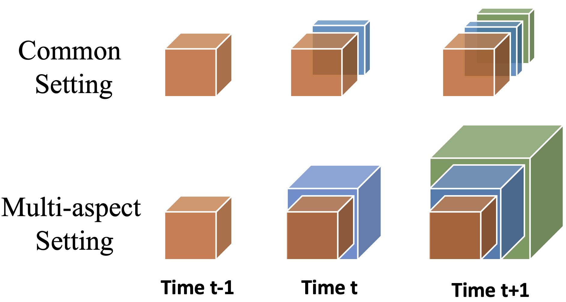
Figure 2: Online Tensor Factorization

Online tensor factorization tries to maintain the factorization results (e.g., CP factors) while the tensor is growing, shown in Fig. 2. Zhou et al. Zhou et al. (2016) proposed an accelerated algorithm for the common setting where only the temporal mode grows. Song et al. (2017) considered the multi-aspect setting where multiple mode grows simultaneously. We discuss the multi-aspect setting below.

Problem 2 (Multi-aspect Online Tensor Factorization).

Suppose tensor $\mathcal{X}^{t-1}\in\mathbb{R}^{I^{t-1}_{1}\times I^{t-1}_{2}\times I^{t-1}_{3}}$ at time $(t-1)$ admits a low-rank approximation, induced by $\mathbf{U}^{t-1}\in\mathbb{R}^{I_{1}^{t-1}\times R}$, $\mathbf{V}^{t-1}\in\mathbb{R}^{I_{2}^{t-1}\times R}$, $\mathbf{W}^{t-1}\in\mathbb{R}^{I_{3}^{t-1}\times R}$, such that

$$\mathcal{X}^{t-1}\approx\llbracket\mathbf{U}^{t-1},\mathbf{V}^{t-1},\mathbf{W}^{t-1}\rrbracket.$$

At time $t$, we want to learn a new set of factors, $\mathbf{U}^{t}\in\mathbb{R}^{I_{1}^{t}\times R},\mathbf{V}^{t}\in\mathbb{R}^{I_{2}^{t}\times R},\mathbf{W}^{t}\in\mathbb{R}^{I_{3}^{t}\times R}$ to approximate the growing new tensor $\mathcal{X}^{t}\in\mathbb{R}^{I^{t}_{1}\times I^{t}_{2}\times I^{t}_{3}}$, which satisfies,

$$x_{i_{1}i_{2}i_{3}}^{t}=x_{i_{1}i_{2}i_{3}}^{t-1},~{}\forall i_{n}\in[1,\cdots,I_{n}^{t-1}],~{}\forall n\in[1,2,3].$$

Unification.

To achieve the existing objective in the literature, we simply reduce our $\mathcal{L}_{\mathrm{E}}$ by changing the L2 regularization into nuclear norm (i.e., the sum of singular values),

$$\mathcal{L}_{\mathrm{reg}}=\gamma_{1}\left\|\mathbf{U}^{t}\right\|_{*}+\gamma_{2}\left\|\mathbf{V}^{t}\right\|_{*}+\gamma_{3}\left\|\mathbf{W}^{t}\right\|_{*},$$

where $\gamma_{n},~{}\forall~{}n\in[1,2,3]$ are the hyperparameters and they sum up to one. This regularization is the convex relaxation of CP rank Song et al. (2017). Then, the objective becomes

$$\mathcal{L}_{\mathrm{E}}= \left\|(\mathcal{X}^{t}-\llbracket\mathbf{U}^{t},\mathbf{V}^{t},\mathbf{W}^{t}\rrbracket)_{\tilde{\Omega}^{t}}\right\|_{F}^{2}$$

$$+\alpha\left\|(\mathcal{Y}^{t-1}-\llbracket\mathbf{U}^{t},\mathbf{V}^{t},\mathbf{W}^{t}\rrbracket)_{\Omega^{t-1}}\right\|_{F}^{2}$$

$$+\beta\left(\gamma_{1}\left\|\mathbf{U}^{t}\right\|_{*}+\gamma_{2}\left\|\mathbf{V}^{t}\right\|_{*}+\gamma_{3}\left\|\mathbf{W}^{t}\right\|_{*}\right),$$

where $\Omega^{t}$ and $\Omega^{t-1}$ are the bounds of the new and previous tensors and $\tilde{\Omega}^{t}=\Omega^{t}\setminus\Omega^{t-1}$ (in this case, $\Omega^{t,\mathrm{old}}=\Omega^{t-1}$) indicates the newly added elements at time $t$. This form is identical to the objective proposed in Song et al. (2017).

In experiment Sec. 5.3, we evaluate on the temporal mode growth setting. Our methods use the L2 regularization as listed in Sec. 3 and follow Algorithm 1.

4.2 Online Tensor Completion

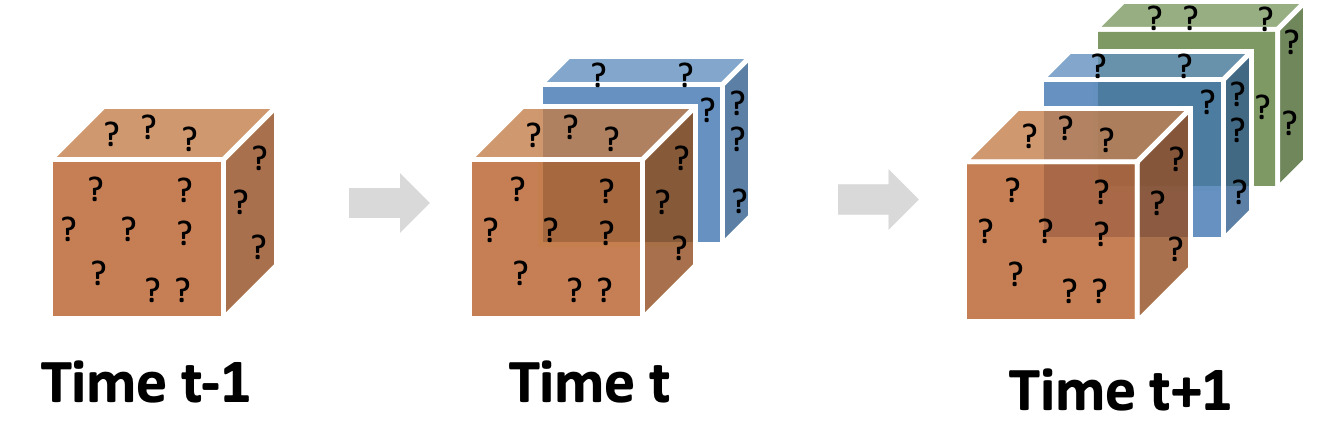
Figure 3: Online Tensor Completion

Online tensor completion studies incomplete tensors, where new incomplete slices will add to the temporal mode. The goal is to effectively compute a new tensor completion result (i.e., CP factors) for the augmented tensor. This problem is studied in Mardani et al. (2015); Kasai (2016, 2019). We show the formulation below.

Problem 3 (Online Tensor Completion).

Suppose $\mathcal{X}^{t-1}$ is the underlying tensor at time $(t-1)$, which admits a low-rank approximation, $\mathbf{U}^{t-1}\in\mathbb{R}^{I_{1}\times R}$, $\mathbf{V}^{t-1}\in\mathbb{R}^{I_{2}\times R}$, $\mathbf{W}^{t-1}\in\mathbb{R}^{I^{t-1}_{3}\times R}$, such that given the mask $\Omega^{t-1}$,

$$\Omega^{t-1}\stackMath\mathbin{\stackinset{c}{0ex}{c}{0ex}{\ast}{\ocircle}}\mathcal{X}^{t-1}\approx\Omega^{t-1}\stackMath\mathbin{\stackinset{c}{0ex}{c}{0ex}{\ast}{\ocircle}}\llbracket\mathbf{U}^{t-1},\mathbf{V}^{t-1},\mathbf{W}^{t-1}\rrbracket.$$

At the time $t$, given a new slice with incomplete entries, i.e., $\Omega_{\Delta}^{t}\stackMath\mathbin{\stackinset{c}{0ex}{c}{0ex}{\ast}{\ocircle}}\mathbf{X}_{\Delta}^{t}\in\mathbb{R}^{I_{1}\times I_{2}}$, the new data is concatenated along the temporal mode (the third-mode) by $\Omega^{t}=[\Omega^{t-1};\Omega^{t}_{\Delta}]$ and $\mathcal{X}^{t}=[\mathcal{X}^{t-1};\mathbf{X}_{\Delta}^{t}]$. We want to update the approximation with $\mathbf{U}^{t}\in\mathbb{R}^{I_{1}\times R}$, $\mathbf{V}^{t}\in\mathbb{R}^{I_{2}\times R}$, $\mathbf{W}^{t}\in\mathbb{R}^{I_{3}^{t}\times R}$, where $I^{t}_{3}=I_{3}^{t-1}+1$, such that

$$\Omega^{t}\stackMath\mathbin{\stackinset{c}{0ex}{c}{0ex}{\ast}{\ocircle}}\mathcal{X}^{t}\approx\Omega^{t}\stackMath\mathbin{\stackinset{c}{0ex}{c}{0ex}{\ast}{\ocircle}}\llbracket\mathbf{U}^{t},\mathbf{V}^{t},\mathbf{W}^{t}\rrbracket.$$

Unification.

To handle this setting, we remove the reconstruction regularizer (second term) from our $\mathcal{L}$ and the reduced version can be transformed into,

$$\mathcal{L}= \sum_{k=1}^{I_{3}^{t}}\left[\alpha\left\|\left(\mathbf{X}^{t,k}-\mathbf{U}^{t}\mathrm{diag}(\mathbf{w}^{t}_{k})\mathbf{V}^{t\top}\right)_{\Omega^{t,k}}\right\|_{F}^{2}+\beta\|\mathbf{w}_{k}^{t}\|_{F}^{2}\right]$$ (12)

$$+\beta\left(\|\mathbf{U}^{t}\|_{F}^{2}+\|\mathbf{V}^{t}\|_{F}^{2}\right),$$

where $\Omega^{t,k}$ and $\mathbf{X}^{t,k}$ indicate the $k$-th slices of the tensor along the temporal mode, and $\mathbf{w}^{t}_{k}$ is the $k$-th row of $\mathbf{W}^{t}$. From Eqn. (12), we could make $\alpha$ exponential decaying w.r.t. time steps (i.e., $\alpha_{k}=\gamma^{I_{3}^{t}-k}$), the $\beta$ within summation be time-variant (i.e., $\beta_{k}=\lambda_{k}\times\gamma^{I_{3}^{t}-k}$) and the $\beta$ outside be $\lambda_{I_{3}^{t}}$, where $\gamma,\{\lambda_{k}\}$ are hyperparameters. We then obtain the identical objective as proposed in Mardani et al. (2015). The experiments are shown in Sec. 5.4.

5 Experiments

In the experiment, we evaluate our model on various settings. Our models are named GOCPT (with the objective $\mathcal{L}$) and $\mbox{{GOCPT}}_{\mathrm{E}}$ (with objective $\mathcal{L}_{\mathrm{E}}$). Dataset statistics are listed in Table 1. More details can be found in appendix C.

Dataset	Format	Setting
JHU Covid	$51\times 3\times 8\times 209$	General (Sec. 5.2)
Patient Claim	$56\times 22\times 10\times 104$	General (Sec. 5.2)
FACE-3D	$112\times 99\times 400$	Factorization (Sec. 5.3)
GCSS	$50\times 422\times 362$	Factorization (Sec. 5.3)
Indian Pines	$145\times 145\times 200$	Completion (Sec. 5.4)
CovidHT	$420\times 189\times 128$	Completion (Sec. 5.4)

Table 1: Data Statistics

5.1 Experimental Setups

Metrics.

The main metric is percentage of fitness (PoF) Acar et al. (2011), which is defined for the factorization or completion problem respectively by (the higher, the better)

$$1-\frac{\|\mathcal{X}-\llbracket\mathbf{A}_{1}\dots\mathbf{A}_{N}\rrbracket\|_{F}}{\|\mathcal{X}\|_{F}}~{}~{}~{}\mbox{or}~{}~{}~{}1-\frac{\|(1-\Omega)\stackMath\mathbin{\stackinset{c}{0ex}{c}{0ex}{\ast}{\ocircle}}(\mathcal{X}-\llbracket\mathbf{A}_{1}\dots\mathbf{A}_{N}\rrbracket)\|_{F}}{\|(1-\Omega)\stackMath\mathbin{\stackinset{c}{0ex}{c}{0ex}{\ast}{\ocircle}}\mathcal{X}\|_{F}},$$

where $\Omega$ and $\mathcal{X}$ are the mask and underlying tensor, $\{\mathbf{A}_{1},\cdots,\mathbf{A}_{N}\}$ are the low-rank CP factors. We also report the total time consumption as an efficiency indicator.

Baselines.

We simulate three different practical scenarios for performance comparison. Since not all existing methods can deal with the three cases, we select representative state-of-the-art algorithms in each scenario for comparison:

• For the general case in Sec. 5.2, most previous models cannot support this setting. We adopt EM-ALS Acar et al. (2011); Walczak and Massart (2001) and CPC-ALS Karlsson et al. (2016) as the compared methods, which follow the similar initialization procedure in Sec. 3.2.

• For the online tensor factorization in Sec. 5.3, we employ OnlineCPD Zhou et al. (2016); MAST Song et al. (2017) and CPStream Smith et al. (2018), which use ADMM and require multiple iterations; RLST Nion and Sidiropoulos (2009), which is designed only for third-order tensors.

• For the online tensor completion in Sec. 5.4, we implement EM-ALS and its variant, called EM-ALS (decay), which assigns exponential decaying weights for historical slices; OnlineSGD Mardani et al. (2015); OLSTEC Kasai (2016, 2019) for comparison.

We compare the space and time complexity of each model in appendix B. All experiments are conduct with 5 random seeds. The mean and standard deviations are reported.

5.2 General Case with Three Evolving Patterns

Datasets and Settings.

We use (i) JHU Covid data Dong et al. (2020) and (ii) proprietary Patient Claim data to conduct the evaluation. The JHU Covid data was collected from Apr. 6, 2020, to Oct. 31, 2020 and the Patient Claim dataset collected weekly data from 2018 to 2019. To mimic tensor value updates on two datasets, we later add random perturbation to randomly selected $2\%$ existing data with value changes uniformly of $[-5\%,5\%]$ at each time step. The leading $50\%$ slices are used as preparation data to obtain the initial factors with rank $R=5$. The results are in Table 2.

Model	JHU Covid Data		Perturbed JHU Covid Data
	Total Time (s)	Avg. PoF	Total Time (s)	Avg. PoF
EM-ALS	1.68 $\pm$ 0.001	0.6805 $\pm$ 0.024	2.13 $\pm$ 0.049	0.6622 $\pm$ 0.047
CPC-ALS	2.14 $\pm$ 0.002	0.6813 $\pm$ 0.028	2.50 $\pm$ 0.013	0.6634 $\pm$ 0.021
$\mbox{{GOCPT}}_{\mathrm{E}}$	1.32 $\pm$ 0.004	0.6897 $\pm$ 0.016	1.72 $\pm$ 0.034	0.6694 $\pm$ 0.045
GOCPT	2.68 $\pm$ 0.002	0.6920 $\pm$ 0.022	3.17 $\pm$ 0.041	0.6827 $\pm$ 0.024
Model	Patient Claim		Perturbed Patient Claim
	Total Time (s)	Avg. PoF	Total Time (s)	Avg. PoF
EM-ALS	4.37 $\pm$ 0.056	0.4458 $\pm$ 0.023	5.35 $\pm$ 0.066	0.4626 $\pm$ 0.021
CPC-ALS	4.74 $\pm$ 0.036	0.5022 $\pm$ 0.021	5.58 $\pm$ 0.009	0.5169 $\pm$ 0.019
$\mbox{{GOCPT}}_{\mathrm{E}}$	2.71 $\pm$ 0.033	0.5299 $\pm$ 0.019	3.27 $\pm$ 0.024	0.5454 $\pm$ 0.017
GOCPT	5.10 $\pm$ 0.037	0.5485 $\pm$ 0.022	5.91 $\pm$ 0.042	0.5577 $\pm$ 0.021

Table 2: Results on General Case

Result Analysis.

Overall, our models show the top fitness performance compared to the baselines, and the variant $\texttt{GOCPT}_{\mathrm{E}}$ shows $20\%$ efficiency improvement over the best model with comparable fitness on both datasets. CPC-ALS and EM-ALS performs similarly on Covid tensor and CPC-ALS works better on the Patient Claim data, while they are inferior to our models in both fitness and efficiency.

5.3 Special Case: Online Tensor Factorization

Dataset and Setups.

We present the evaluation on low-rank synthetic data. In particular, we generate three CP factors from uniform $[0,1]$ distribution and then construct a low-rank tensor $(I_{1},I_{2},I_{3},R)=(50,50,500,5)$. We use the leading $10\%$ slices along the (third) temporal mode as preparation; then, we add one slice at each time step to simulate mode growth. We report the mean values in Figure 4.

Also, we show that our GOCPT can provide better fitness than all baselines and $\mbox{{GOCPT}}_{\mathrm{E}}$ outputs comparable fitness with state of the art efficiency on two real-world datasets: (i) ORL Database of Faces (FACE-3D) and (ii) Google Covid Search Symptom data (GCSS). The result tables are moved to appendix C.3 due to space limitation.

5.4 Special Case: Online Tensor Completion

Datasets and Setups.

Using the same synthetic data described in Sec. 5.3, we randomly mask out $98\%$ of the entries and follow the same data preparation and mode growth settings. The results of mean curves are shown in Fig. 4.

We also evaluate on two real-world datasets: (i) Indian Pines hyperspectral image dataset and (ii) a proprietary Covid disease counts data: location by disease by date, we call it the health tensor (CovidHT), and the results (refer to appendix C.4) show that GOCPT has the better fitness and $\mbox{{GOCPT}}_{\mathrm{E}}$ has decent fitness with good efficiency.

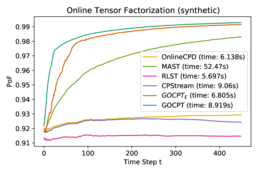
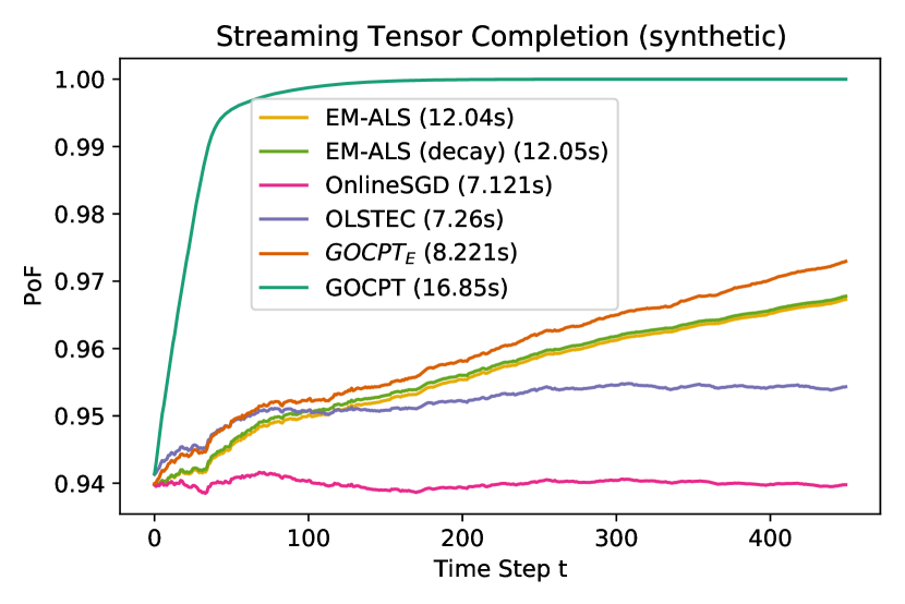
Figure 4: Performance Comparison on Special Cases

6 Conclusion

This paper proposes a generalized online tensor factorization and completion framework, called GOCPT, which can support various tensor evolving patterns and unifies existing online tensor formulations. Experiments confirmed that our GOCPT can show good performance on the general setting, where most previous methods cannot support. Also, our GOCPT provides comparable or better performance in each special setting. The GOCPT package is currently open-sourced.

Appendix A Matrix and Tensor Algebra, Notations

Table 3: Notations used in GOCPT

Symbols	Descriptions
$\odot$	tensor Khatri-Rao product
$\stackMath\mathbin{\stackinset{c}{0ex}{c}{0ex}{\ast}{\ocircle}}$	tensor Hadamard product
$\llbracket\cdot\rrbracket$	tensor Kruskal product
$R$	tensor CP rank
$\Omega^{t}\in\mathbb{R}^{I_{1}^{t}\times\cdots I_{N}^{t}}$	tensor (observation) mask
$\tilde{\Omega}^{t},\tilde{\Omega}^{t,old}$	mask for new data and old data
	where we have $\tilde{\Omega}^{t}\bigcup\tilde{\Omega}^{t,old}=\Omega^{t}$
$\mathcal{X}^{t}\in\mathbb{R}^{I_{1}^{t}\times\cdots I_{N}^{t}}$	the underlying tensor
$\mathcal{Y}^{t}\in\mathbb{R}^{I_{1}^{t}\times\cdots I_{N}^{t}}$	low-rank approximation of $\mathcal{X}^{t}$
$\mathbf{A}^{n,t}\in\mathbb{R}^{I_{n}^{t}\times R},~{}\forall n$	the factor matrices
$\mathbf{a}_{i_{n}}^{n,t}\in\mathbb{R}^{1\times R},~{}\forall n,i_{n}$	the $i_{n}$-th row of the factor matrices
$\mathbf{U}^{n,t}\in\mathbb{R}^{I_{n}^{t-1}\times R},~{}\forall n$	the upper block matrices
$\mathbf{L}^{n,t}\in\mathbb{R}^{(I_{n}^{t}-I_{n}^{t-1})\times R},~{}\forall n$	the lower block matrices
$\mathbf{P}_{i_{n}}^{n,t}\in\mathbb{R}^{R\times R},\mathbf{q}_{i_{n}}^{n,t}\in\mathbb{R}^{1\times R}$	auxiliary variables
$\mathbf{P}_{\mathbf{U}}^{n,t}\in\mathbb{R}^{R\times R},\mathbf{Q}_{\mathbf{U}}^{n,t}\in\mathbb{R}^{I_{n}^{t-1}\times R}$	auxiliary variables for $\mathbf{U}^{n,t}$
$\mathbf{P}_{\mathbf{L}}^{n,t}\in\mathbb{R}^{R\times R},\mathbf{Q}_{\mathbf{L}}^{n,t}\in\mathbb{R}^{(I_{n}^{t}-I_{n}^{t-1})\times R}$	auxiliary variables for $\mathbf{L}^{n,t}$

Note that (i) notation with superscript ^t means at time $t$; (ii) notations with $\hat{}$ means the initialized value or the estimated value.

Kronecker Product.

One important operation for matrices is the Kronecker product. For $\mathbf{A}\in\mathbb{R}^{I\times J}$ and $\mathbf{B}\in\mathbb{R}^{K\times L}$, their Kronecker product is defined by (each block is a scalar times matrix)

$$\small\mathbf{A}\otimes\mathbf{B}=\begin{bmatrix}a_{11}\mathbf{B}&a_{12}\mathbf{B}&\cdots&a_{1J}\mathbf{B}\\ a_{21}\mathbf{B}&a_{22}\mathbf{B}&\cdots&a_{2J}\mathbf{B}\\ \vdots&\vdots&\cdots&\vdots\\ a_{I1}\mathbf{B}&a_{I2}\mathbf{B}&\cdots&a_{IJ}\mathbf{B}\end{bmatrix}\in\mathbb{R}^{IK\times JL}.$$

Khatri–Rao Product.

Khatri-Rao product is another important product for matrices, specifically, for matrices with same number of columns. The Khatri-Rao product of $\mathbf{A}\in\mathbb{R}^{I\times J}$ and $\mathbf{B}\in\mathbb{R}^{K\times J}$ can be viewed as column-wise Kroncker product,

$$\mathbf{A}\odot\mathbf{B}=\begin{bmatrix}\mathbf{a}^{(1)}\otimes\mathbf{b}^{(1)},\mathbf{a}^{(2)}\otimes\mathbf{b}^{(2)},\cdots,\mathbf{a}^{(L)}\otimes\mathbf{b}^{(L)}\end{bmatrix},$$

where $\mathbf{a}^{(k)}$ and $\mathbf{b}^{(k)}$ are the $k$-th column of $\mathbf{A}$ and $\mathbf{B}$, and $\mathbf{A}\odot\mathbf{B}\in\mathbb{R}^{IK\times L}$.

Tensor Unfolding.

This operation is to matricize a tensor along one mode. For tensor $\mathcal{X}\in\mathbb{R}^{I_{1}\times I_{2}\times I_{3}}$, we could unfold it along the first mode into a matrix $\mathbf{X}_{1}\in\mathbb{R}^{I_{1}\times I_{2}I_{3}}$. Specifically, each row of $\mathbf{X}_{1}$ is a vectorization of a slice in the original tensor; we have

$$\mathbf{X}_{1}(i,j\times I_{3}+k)=\mathcal{X}(i,j,k),~{}\forall i,j,k.$$

Here, to reduce clutter, we use Matlab-style notation to index the value. Similarly, for the unfolding operation along the second or third mode, we have

$$\mathbf{X}_{2}(j,i\times I_{3}+k) =\mathcal{X}(i,j,k)\in\mathbb{R}^{I_{2}\times I_{1}I_{3}},~{}\forall i,j,k,$$

$$\mathbf{X}_{3}(k,i\times I_{2}+j) =\mathcal{X}(i,j,k)\in\mathbb{R}^{I_{3}\times I_{1}I_{2}},~{}\forall i,j,k.$$

Hadamard Product.

The Hadamard product is the element-wise product for tensors of the same size. For example, the Hadamard product of two $3$-mode tensors $\mathcal{X},\mathcal{Y}\in\mathbb{R}^{I_{1}\times I_{2}\times I_{3}}$ is

$$\mathcal{Z}=\mathcal{X}\stackMath\mathbin{\stackinset{c}{0ex}{c}{0ex}{\ast}{\ocircle}}\mathcal{Y}\in\mathbb{R}^{I_{1}\times I_{2}\times I_{3}}.$$

Canonical Polyadic (CP) Factorization.

One of the common compression methods for tensors is CP factorization Hitchcock [1927]; Carroll and Chang [1970], also called CANDECOMP/PARAFAC (CP) factorization, which represents a tensor by multiple rank-one components. For example, let $\mathcal{X}\in\mathbb{R}^{I_{1}\times I_{2}\times I_{3}}$ be an arbitrary $3$-order tensor of CP-rank $R$, then it can be expressed exactly by factor matrices $\mathbf{U}\in\mathbb{R}^{I_{1}\times R},\mathbf{V}\in\mathbb{R}^{I_{2}\times R},\mathbf{W}\in\mathbb{R}^{I_{3}\times R}$ as

$$\mathcal{X}=\sum_{r=1}^{R}\mathbf{u}^{(r)}\circ\mathbf{v}^{(r)}\circ\mathbf{w}^{(r)}=\llbracket\mathbf{U},\mathbf{V},\mathbf{W}\rrbracket,$$

where $\circ$ is vector outer product, $\mathbf{u}^{(r)},\mathbf{v}^{(r)},\mathbf{w}^{(r)}$ are the $r$-th column vectors.

Appendix B Complexity Analysis

Follow the notations in Section 2 of main paper, we analyze the space and time complexity of the optimization algorithm. Assume the CP-rank $R$ satisfies: $I_{n}^{t}\gg R,~{}\forall t,~{}\forall n$. Let $S^{t}=\sum_{n=1}^{N}I_{n}^{t}$, $P^{t}=\prod_{n=1}^{N}I_{n}^{t}$, and $nnz(\cdot)$ indicates the number of non-zero entries.

Space Complexity.

The space complexity records the storage needed for input at time $t$. For objective $\mathcal{L}$, we need the previous factors, $S^{t-1}R$, and the current data, $nnz(\Omega^{t})$ (note that, nonzero entries of the mask indicates the observed data). In total, $S^{t-1}R+nnz(\Omega^{t})$ is the input size; for the efficient version $\mathcal{L}_{\mathrm{E}}$, the old unchanged data is not needed. Therefore, the input size is $S^{t-1}R+nnz(\tilde{\Omega}^{t})$.

Time Complexity.

For time complexity, the analysis is under the sparse or dense strategies in Sec 3.2 of the main paper.

• Sparse strategy. In Eqn. (10), the overall cost of computing $\mathbf{P}^{n,t}_{i_{n}}$ is $\mathcal{O}(nnz(\Omega^{t})NR(N+R))$; In Eqn. (11), the overall cost of computing $\mathbf{q}^{n,t}_{i_{n}}$ is $\mathcal{O}(nnz(\Omega^{t})N^{2}R)$; the cost of matrix inverse for all $\mathbf{P}^{n,t}_{i_{n}}$ is $\mathcal{O}(S^{t}R^{3})$ by Cholesky decomposition (which could be omitted since $nnz(\Omega^{t})\gg S^{t}$). Overall, the time complexity for $\mathcal{L}$ is $\mathcal{O}(nnz(\Omega^{t})NR(N+R))$. The time complexity for $\mathcal{L}_{\mathrm{E}}$ is $\mathcal{O}(nnz(\tilde{\Omega}^{t})NR(N+R))$.

• Dense strategy. First, the cost of imputing the tensor is $\mathcal{O}(P^{t}R)$. Then, in Eqn. (13), the overall cost of MTTKRP ($\mathbf{Q}^{n,t}_{\mathbf{U}}$ and $\mathbf{Q}^{n,t}_{\mathbf{L}}$) is $\mathcal{O}(NP^{t}R)$; the cost of computing $\mathbf{P}^{n,t}_{\mathbf{U}}$ and $\mathbf{P}^{n,t}_{\mathbf{L}}$ is $\mathcal{O}(S^{t}R^{2})$ and the cost of calculating their inverse is $\mathcal{O}(NR^{3})$ (these two quantity could be omitted since $P^{t}\gg S^{t},P^{t}\gg R^{2}$). The dominant complexity are imputation and MTTKRP, which sum up to $\mathcal{O}(NP^{t}R)$ for $\mathcal{L}$. The cost of $\mathcal{L}_{\mathrm{E}}$ is $\mathcal{O}(NP^{t}R/I_{n}^{t})$ with only mode growth (one new slice at a time), but it can be up to $\mathcal{O}(NP^{t}R)$ in more complex scenarios.

For a comprehensive comparison, we listed the space and time complexity of all baselines in Table 4, while for different settings, the baselines are different.

Model	Space Complexity	Time Complexity
For Sec. 5.2 (the general setting) and Sec. 5.4 (the completion setting):
EM-ALS	$nnz(\Omega^{t})+(\bar{S}+I_{N})R$	$\mathcal{O}(NR\bar{P}I_{N})$
CPC-ALS	$nnz(\Omega^{t})+(\bar{S}+I_{N})R$	$\mathcal{O}(nnz(\Omega^{t})NR(N+R))$
OnlineSGD	$nnz(\tilde{\Omega}^{t})+(\bar{S}+I_{N})R$	$\mathcal{O}(nnz(\tilde{\Omega}^{t})NR(N+R))$
OLSTEC	$nnz(\tilde{\Omega}^{t})+(\bar{S}R+2\bar{S}+I_{N})R$	$\mathcal{O}(nnz(\tilde{\Omega}^{t})NR(N+R))$
$\mbox{{GOCPT}}_{\mathrm{E}}$	$nnz(\tilde{\Omega}^{t})+(\bar{S}+I_{N})R$	$\mathcal{O}(nnz(\tilde{\Omega}^{t})NR(N+R))$
GOCPT	$nnz(\Omega^{t})+(\bar{S}+I_{N})R$	$\mathcal{O}(nnz(\Omega^{t})NR(N+R))$
For Sec. 5.3 (the factorization setting):
OnlineCPD	$\bar{P}+(2\bar{S}+I_{N})R+(N-1)R^{2}$	$\mathcal{O}(NR\bar{P})$
MAST	$\bar{P}+3(\bar{S}+I_{N})R$	$\mathcal{O}(NR\bar{P})$
RLST	$\bar{P}+(\bar{S}+2\bar{P}+I_{N})R+2R^{2}$	$\mathcal{O}(R^{2}\bar{P})$
CPStream	$\bar{P}+(\bar{S}+I_{N}+R)R$	$\mathcal{O}(NR\bar{P})$
$\mbox{{GOCPT}}_{\mathrm{E}}$	$\bar{P}+(\bar{S}+I_{N})R$	$\mathcal{O}(NR\bar{P})$
GOCPT	$\bar{P}I_{N}+(\bar{S}+I_{N})R$	$\mathcal{O}(NR\bar{P}I_{N})$

Table 4: Complexity per iteration at Time $t$, where $\bar{P}=P/I_{N},\bar{S}=S-I_{N}$ (refer to Sec. B) and we remove the superscript ^t whenever there is no ambiguity.

Appendix C Additions for Experiments

All experiments use $R=5$ and are implemented by Python 3.8.5, Numpy 1.19.1 and the experiments are conducted on a Linux workstation with 256 GB memory, 32 core CPUs (3.70 GHz, 128 MB cache) In our experiments of the main text, we use the sparse strategy for the general case and the tensor completion case and use dense strategy for the factorization case.

Average PoF (Avg. PoF). Note that, in section 5.2 of the main paper, the Avg. PoF is calculated by averaging the PoF scores over the time steps (remember that we calculate a PoF score per time step), and the mean and standard deviation values are calculated on five runs with different random seeds.

C.1 Datasets Description

• JHU Covid Dataset. As mentioned in the main text, this dataset Dong et al. [2020] was collected from Apr. 6, 2020 to Oct. 31, 2020. We model the data as a fourth-order tensor and treat 3 categories: new cases, deaths, and hospitalization as the feature dimension. The collected data covers 51 states across the US. This data contains 209 generation dates (GD) and 8 loading dates (LD) for each data point. The leading $50\%$ slices (before Jul. 16) are used as preparation data to obtain the initial factors. The reflection of three evolving patterns: at each timestamp, the GD will increase by 1 and the LD dimension will be filled accord to how previous data is received. Later, we add random perturbations to randomly selected $2\%$ eisting data with value changes uniformly of $[-5\%,5\%]$ at each time step.

• Patient Claim Data. This dataset can also be modeled as a fourth-order tensor, which contains 56 states, 22 disease categories, 10 LD’s (for the delayed updates), and 104 GD’s (104 weeks over the year 2018 and 2019, there is one generated service data point for each week). The leading $50\%$ slices (data of year 2018) are used as preparation data to obtain the initial factors. The reflection of three evolving patterns: at each timestamp, the GD will increase by 1 and the LD dimension will be filled accordingly. Later, at each time step, we add random perturbations to randomly selected $2\%$ eisting data with value changes uniformly of $[-5\%,5\%]$.

  For the above two datasets, the GD mode is the growing mode (referring to change type (i)), and the LD (delayed updates) causes the incompleteness of previous tensor slices, while the incomplete slices will be filled in later dates (referring to change type (ii)). By fixing the first and the second modes, we show a diagram (figure below) of how the GD and LD evolve. At each time step, a new GD is generated while the LDs for the previous GD’s can be filled (assuming that all GD’s have the same number of LDs in total). A special setting is discussed in a recent paper Qian et al. [2021].

  

  Additionally, to simulate change type (iii) on these two datasets, we add random perturbations to the existing tensor elements in the experiments.

• FACE-3D. ORL Database of Faces contains 400 shots of face images with size 112 pixels by 99 pixels. To construct a third-order tensor, we treat each shot as a slice and concatenate them together. The first $10\%$ leading shots are used as preparation data.

• GCSS. This is a public dataset containing google covid-19 symptom search results during the complete year 2020. The data can be viewed as a third-order tensor: 50 states, 422 keywords, and 362 days. The first $10\%$ leading dates are used as preparation data.

• Indian Pines. This is also an open dataset containing 200 shots of hyperspectral images with size 145 pixels by 145 pixels. The data is also modeled as a third-order tensor. We manually mask out $98\%$ of the tensor elements for the online tensor completion problem. Later, the masked out entries are used as ground truth to evaluate our completion results. The first $10\%$ leading images are used as preparation data.

• CovidHT. This is a proprietary covid-19 related disease tensor with 420 zip codes, 189 disease categories, and 128 dates. We model it as a third-order tensor. Similar to the Indian Pines datasets, we manually mask out $98\%$ of the tensor elements for later evaluation, and the first $10\%$ leading shots are used as preparation data.

C.2 Hyperparameter settings

Our framework has two hyperparameters, the first one is $\beta$, which is the weight for L2 regularization. We set $\beta=10^{-5}$ for all experiments and it does not change w.r.t. time step $t$. Another hyperparameter is $\alpha$, controlling the importance of historical reconstruction. Let us set $I^{t}$ to be the dimension of the growing mode. We listed the $\alpha$ used in the experiments in Table 5. There are several advices on choosing the hyperparameters: (i) for any settings included with real-world datasets, the $\alpha$ can be chosen based on the simulation results of the synthetic data; (ii) we keep a larger $\alpha$ for the real-world data (in factorization case), since the real data is usually not smooth and the statistics from old slices to new slices could change. A larger $\alpha$ would make transition from time $(t-1)$ to time $t$ more smooth, which makes the final results more stable; (iii) compared to GOCPT, our $\mbox{{GOCPT}}_{\mathrm{E}}$ does not keep the historical data, so it relies on the historical reconstruction more, then we set a larger $\alpha$, which is 100 times the $\alpha$ for GOCPT. The details for different settings can refer to: the general case (Sec. 5.2 of main text), factorization case (Sec. 5.3 of main text), completion cases (Sec. 5.4 of main text).

Settings	GOCPT	$\mbox{{GOCPT}}_{\mathrm{E}}$
general case	$\alpha=0.02/I^{t}$	$\alpha=2/I^{t}$
factorization case	$\alpha=0.02/I^{t}$ for synthetic data	$\alpha=2/I^{t}$ for synthetic data
	$\alpha=2/I^{t}$ for real data	$\alpha=min(1,200/I^{t})$ for real data
completion case	$\alpha=0.005/I^{t}$	$\alpha=0.5/I^{t}$

Table 5: Hyperparameter $\alpha$ Settings for All Experiments

C.3 Exp. for Online Tensor Factorization

The setting is discussed in the main paper, however, we move the result table here due to space limitation.

Note that the contribution of our model is to (a) provide a unified framework and can handle both online tensor factorization and completion (previous models are designed only for either); (b) show that our model can provide comparable or better performance over all baselines in all settings. Here, section C.3 and C.4 are to empirically show (b).

Model	FACE-3D		GCSS
	Total Time (s)	Avg. PoF	Total Time (s)	Avg. PoF
OnlineCPD	13.61 $\pm$ 0.040	0.7447 $\pm$ 1.129e-3	26.38 $\pm$ 0.035	0.9258 $\pm$ 3.053e-4
MAST	98.52 $\pm$ 0.012	0.7464 $\pm$ 1.405e-3	159.21 $\pm$ 0.192	0.9278 $\pm$ 2.437e-4
RLST	13.33 $\pm$ 0.033	0.7216 $\pm$ 2.342e-3	26.64 $\pm$ 0.004	0.6725 $\pm$ 3.653e-2
CPStream	18.35 $\pm$ 0.005	0.7446 $\pm$ 1.281e-3	43.61 $\pm$ 0.112	0.9256 $\pm$ 5.192e-4
$\mbox{{GOCPT}}_{\mathrm{E}}$	13.77 $\pm$ 0.165	0.7452 $\pm$ 1.208e-3	26.75 $\pm$ 0.094	0.9270 $\pm$ 1.022e-4
GOCPT	17.14 $\pm$ 0.071	0.7473 $\pm$ 1.315e-3	34.17 $\pm$ 0.338	0.9297 $\pm$ 3.203e-4

Table 6: Results for Online Tensor Factorization

Result Analysis.

On the real data, OnlineCPD and our $\mbox{{GOCPT}}_{\mathrm{E}}$ show great fitness and the best efficiency. Though GOCPT presents the best fitness score, it is relatively slower than the best model. The baselines MAST and CPStream are expensive since they use ADMM to iteratively update the factors within each time step, which is time-consuming.

C.4 Exp. for Online Tensor Completion

Due to space limitation, we move the experimental results here and give result summary in the main text.

Model	Indian Pines		CovidHT
	Total Time (s)	Avg. PoF	Total Time (s)	Avg. PoF
EM-ALS	17.15 $\pm$ 0.022	0.8839 $\pm$ 5.696e-4	25.71 $\pm$ 0.148	0.5432 $\pm$ 2.317e-2
EM-ALS (decay)	17.05 $\pm$ 0.014	0.8845 $\pm$ 5.452e-4	25.69 $\pm$ 0.115	0.5463 $\pm$ 2.314e-2
OnlineSGD	11.33 $\pm$ 0.025	0.8576 $\pm$ 3.502e-4	15.99 $\pm$ 0.061	0.4422 $\pm$ 1.185e-2
OLSTEC	11.32 $\pm$ 0.014	0.8864 $\pm$ 7.447e-5	16.05 $\pm$ 0.141	0.6503 $\pm$ 7.041e-3
$\mbox{{GOCPT}}_{\mathrm{E}}$	11.82 $\pm$ 0.031	0.8923 $\pm$ 5.083e-4	16.44 $\pm$ 0.039	0.6612 $\pm$ 1.321e-2
GOCPT	19.89 $\pm$ 0.545	0.8970 $\pm$ 1.281e-3	27.92 $\pm$ 0.091	0.6792 $\pm$ 2.602e-2

Table 7: Results for Online Tensor Completion

Result Analysis.

On the real-world data, baseline OLSTEC and our $\mbox{{GOCPT}}_{\mathrm{E}}$ show decent performance, and they both outperform other baseline methods in terms of both fitness and speed, though GOCPT has the best fitness score consistently.

C.5 Discussion on Different Evolving Patterns

Here, we summarize some intuitions and conclusions for the evolving patterns.

• Mode growth may lead to better or poor PoF based on data quality in new dimensions. With more filled missing values, PoF will intuitively increase. These two patterns will increase the running time because the data size (or dimension size) increases.

• According to Table 2 of the main paper, with the additional value update pattern (perturbed version), the running time of all models increases slightly while the final PoF may be improved or not (based on how good the updated value is).

C.6 Ablation Study on Mask Density

This section evaluates the performance of sparse and dense strategies in Sec. 3.2. We experiment on Indian Pines dataset with the full tensors and generate random masks with six density levels. Both strategies run for 25 iterations. We plot the running time versus PoF metric in Fig. 5.

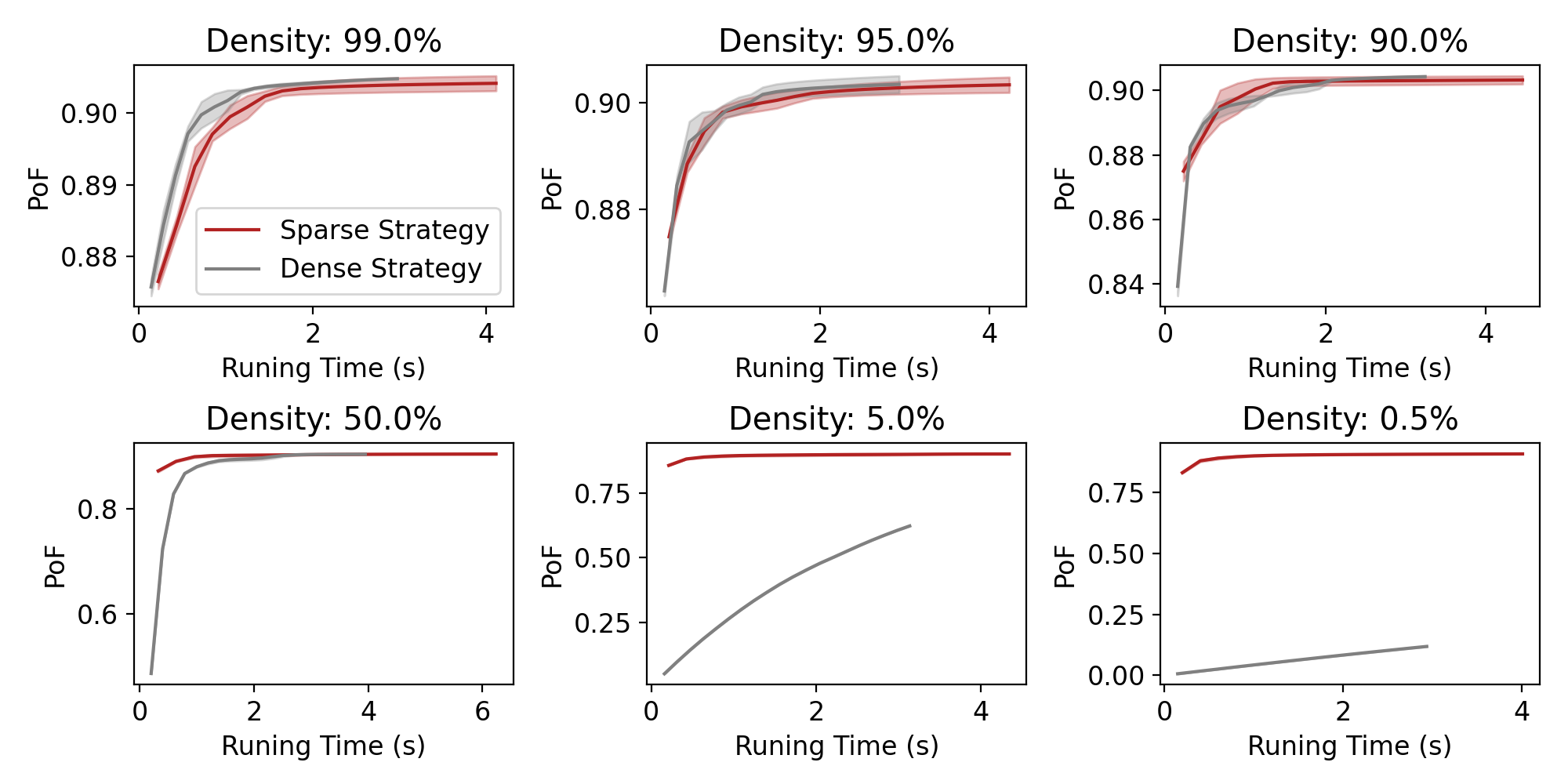
Figure 5: Comparison with Different Density on Mask

Result Analysis.

We observe that dense strategy works well and more efficiently on masks with high density while the sparse strategy is more advantageous when the density is low. Thus, we use the sparse strategy for the general case in Sec. 5.2 and completion case in Sec. 5.4, and use the dense strategy (without the imputation step) for common factorization setting in Sec. 5.3. Note that, our models run either strategy for one iteration per time step.

References

- Acar et al. [2011] Evrim Acar, Daniel M Dunlavy, Tamara G Kolda, and Morten Mørup. Scalable tensor factorizations for incomplete data. Chemometrics and Intelligent Laboratory Systems, 106(1):41–56, 2011.
- Cai et al. [2015] Yongjie Cai, Hanghang Tong, Wei Fan, Ping Ji, and Qing He. Facets: Fast comprehensive mining of coevolving high-order time series. In Proceedings of the 21th ACM SIGKDD International Conference on Knowledge Discovery and Data Mining, pages 79–88, 2015.
- Carroll and Chang [1970] J Douglas Carroll and Jih-Jie Chang. Analysis of individual differences in multidimensional scaling via an n-way generalization of “eckart-young” decomposition. Psychometrika, 1970.
- Dong et al. [2020] Ensheng Dong, Hongru Du, and Lauren Gardner. An interactive web-based dashboard to track covid-19 in real time. The Lancet infectious diseases, 20(5):533–534, 2020.
- Du et al. [2018] Yishuai Du, Yimin Zheng, Kuang-chih Lee, and Shandian Zhe. Probabilistic streaming tensor decomposition. In 2018 IEEE International Conference on Data Mining (ICDM), pages 99–108. IEEE, 2018.
- Fang et al. [2021] Shikai Fang, Robert M Kirby, and Shandian Zhe. Bayesian streaming sparse tucker decomposition. In Proceedings of the 37th Conference on Uncertainty in Artificial Intelligence (UAI), 2021.
- Gilman and Balzano [2020] Kyle Gilman and Laura Balzano. Grassmannian optimization for online tensor completion and tracking with the t-svd. arXiv preprint arXiv:2001.11419, 2020.
- Hitchcock [1927] Frank L Hitchcock. The expression of a tensor or a polyadic as a sum of products. Journal of Mathematics and Physics, 6(1-4):164–189, 1927.
- Hong et al. [2020] David Hong, Tamara G Kolda, and Jed A Duersch. Generalized canonical polyadic tensor decomposition. SIAM Review, 62(1):133–163, 2020.
- Karlsson et al. [2016] Lars Karlsson, Daniel Kressner, and André Uschmajew. Parallel algorithms for tensor completion in the cp format. Parallel Comput., 57(C), 2016.
- Kasai [2016] Hiroyuki Kasai. Online low-rank tensor subspace tracking from incomplete data by cp decomposition using recursive least squares. In 2016 IEEE International Conference on Acoustics, Speech and Signal Processing (ICASSP), pages 2519–2523. IEEE, 2016.
- Kasai [2019] Hiroyuki Kasai. Fast online low-rank tensor subspace tracking by cp decomposition using recursive least squares from incomplete observations. Neurocomputing, 347:177–190, 2019.
- Mardani et al. [2015] Morteza Mardani, Gonzalo Mateos, and Georgios B Giannakis. Subspace learning and imputation for streaming big data matrices and tensors. IEEE TSP, 63(10):2663–2677, 2015.
- Najafi et al. [2019] Mehrnaz Najafi, Lifang He, and S Yu Philip. Outlier-robust multi-aspect streaming tensor completion and factorization. In IJCAI, 2019.
- Nimishakavi et al. [2018] Madhav Nimishakavi, Bamdev Mishra, Manish Gupta, and Partha Talukdar. Inductive framework for multi-aspect streaming tensor completion with side information. In Proceedings of the 27th ACM International Conference on Information and Knowledge Management, pages 307–316, 2018.
- Nion and Sidiropoulos [2009] Dimitri Nion and Nicholas D Sidiropoulos. Adaptive algorithms to track the parafac decomposition of a third-order tensor. IEEE Transactions on Signal Processing, 57(6):2299–2310, 2009.
- Phipps et al. [2021] Eric Phipps, Nick Johnson, and Tamara G Kolda. Streaming generalized canonical polyadic tensor decompositions. arXiv preprint arXiv:2110.14514, 2021.
- Qian et al. [2021] Cheng Qian, Nikos Kargas, Cao Xiao, Lucas Glass, Nicholas Sidiropoulos, and Jimeng Sun. Multi-version tensor completion for time-delayed spatio-temporal data. IJCAI, 2021.
- Smith et al. [2018] Shaden Smith, Kejun Huang, Nicholas D Sidiropoulos, and George Karypis. Streaming tensor factorization for infinite data sources. In Proceedings of the 2018 SIAM International Conference on Data Mining, pages 81–89. SIAM, 2018.
- Song et al. [2017] Qingquan Song, Xiao Huang, Hancheng Ge, James Caverlee, and Xia Hu. Multi-aspect streaming tensor completion. In Proceedings of the 23rd ACM SIGKDD International Conference on Knowledge Discovery and Data Mining, pages 435–443, 2017.
- Sun et al. [2006] Jimeng Sun, Dacheng Tao, and Christos Faloutsos. Beyond streams and graphs: dynamic tensor analysis. In Proceedings of the 12th ACM SIGKDD international conference on Knowledge discovery and data mining, pages 374–383, 2006.
- Walczak and Massart [2001] Beata Walczak and DL Massart. Dealing with missing data: Part i. Chemometrics and Intelligent Laboratory Systems, 58(1):15–27, 2001.
- Xiao et al. [2018] Houping Xiao, Fei Wang, Fenglong Ma, and Jing Gao. eotd: An efficient online tucker decomposition for higher order tensors. In 2018 IEEE International Conference on Data Mining (ICDM). IEEE, 2018.
- Yang et al. [2021] Chaoqi Yang, Navjot Singh, Cao Xiao, Cheng Qian, Edgar Solomonik, and Jimeng Sun. Mtc: Multiresolution tensor completion from partial and coarse observations. KDD, 2021.
- Zhou et al. [2016] Shuo Zhou, Nguyen Xuan Vinh, James Bailey, Yunzhe Jia, and Ian Davidson. Accelerating online cp decompositions for higher order tensors. In In SIGKDD, pages 1375–1384, 2016.
- Zhou et al. [2018] Shuo Zhou, Sarah Erfani, and James Bailey. Online cp decomposition for sparse tensors. In 2018 IEEE ICDM. IEEE, 2018.