shapes \usetikzlibrarysnakes \usetikzlibraryshapes.geometric
Computing solution space properties of combinatorial optimization problems via generic tensor networks
Abstract
We introduce a unified framework to compute the solution space properties of a broad class of combinatorial optimization problems. These properties include finding one of the optimum solutions, counting the number of solutions of a given size, and enumeration and sampling of solutions of a given size. Using the independent set problem as an example, we show how all these solution space properties can be computed in the unified approach of generic tensor networks. We demonstrate the versatility of this computational tool by applying it to several examples, including computing the entropy constant for hardcore lattice gases, studying the overlap gap properties, and analyzing the performance of quantum and classical algorithms for finding maximum independent sets.
keywords:
solution space property, tensor networks, maximum independent set, independence polynomial, generic programming, combinatorial optimization15A69, 05C31, 14N10
1 Introduction
An important class of problems in graph theory and combinatorial optimization can be formulated as satisfiability problems involving constraints specified over a vertex and its neighborhood. These problems include, for example, the independent set problem, the cutting problem, dominating set, set packing, set covering, vertex coloring, K-SAT, the clique problem, and the vertex cover problem [47]. These problems have a wide range of applications in scheduling, logistics, wireless networks and telecommunication, and computer vision, among others [13, 59]. Finding an optimum solution for these problems is typically NP-hard in the worst case [36].
In this Article, we introduce a unified framework to compute a broad class of properties associated with the solutions of these problems, beyond just finding an optimum solution. We call them solution space properties. In practice, these can be much harder to compute (corresponding e.g. to #P-complete class [47]). However, these properties can be crucial for understanding detailed properties of hard combinatorial optimization problems. For example, for the independent set problem, these solution space properties can include not only the maximum or minimum independent set size but also the number of sets at a given size, enumeration of all sets at a given size, and direct sampling of such sets when they are too large to be fit into memory. They can be used to understand the hardness of finding an optimum solution for a given problem instance and the performance of a specific solver. For example, the number of configurations at different sizes can inform how likely a simulated annealing algorithm will be trapped in local minima at certain sizes [60]. The pair-wise Hamming distance distribution of configurations at a given size can indicate the presence or absence of the overlap gap property [28, 27], which can be used to bound the performance of local optimization algorithms. In a recent experiment based on a Rydberg atom array quantum computer, the counting and the configuration space connectivity information was used to find maximum independent set (MIS) problem instances that are hard for simulated annealing and to evaluate the corresponding quantum algorithm performance [19]. The need to understand these important aspects of combinatorial optimization motivates us to find methodologies to compute these solution space properties.
To this end, we show how to obtain all of these seemingly unrelated properties in a unified approach using generic tensor networks. Tensor networks are a computational model widely used in condensed matter physics [48], quantum computing [46], big data [15], mathematics [49] and combinatorial optimization [9, 8, 40]. They are also known as the sum-product networks in probabilistic modeling [10] or einsum in linear algebra libraries such as NumPy [34]. Recent progress in simulating quantum circuits with tensor networks [33, 50, 38] makes it possible to contract a randomly structured sparse tensor network with up to thousands of tensors in a reasonable time. In previous studies, the data types of the tensor elements are typically restricted to standard number types such as real numbers and complex numbers. Here, we extend to generic tensor networks by generalizing the tensor element data types to any type that has the algebraic structure of a commutative semiring. In what follows, for clarity of presentation, we focus on the independent set problem in the main text, and show how to compute the solution space properties for other combinatorial optimization problems in Appendix B. The latter includes cutting, matching, vertex coloring, satisfiability, dominating set, set packing, set covering, and the clique problem.
The paper is organized as follows. We first introduce the basic concepts of tensor networks and generic programming in Section 2 and Section 3. Then we show how to reduce the independent set problem to a tensor network contraction problem in Section 4. Subsequently, we explain how to engineer the element types to compute various solution space properties in Section 6, Section 7, and Section 8. Lastly, we provide three example applications in Section 9 to demonstrate the versatility of our tool. A benchmark to demonstrate the performance of our algorithms can be found in both the Appendix F and the code repository [1].
2 Tensor networks
A tensor network is a multi-linear map from a collection of labelled tensors to an output tensor. It is formally defined as follows.
Definition 2.1 (Tensor Network [16, 48]).
A tensor network is a multi-linear map specified by a triple of , where is a set of symbols (or labels), is a set of tensors as the inputs, and is a string of symbols labelling the output tensor. Each is labelled by a string , where is the rank of . The multi-linear map or the contraction on this triple is
| (1) |
where the summation runs over all possible configurations over the set of symbols absent in the output tensor.
For example, the matrix multiplication can be specified as a tensor network
| (2) |
where and are input matrices (two-dimensional tensors), and are labels associated to the output. The contraction is defined as , where the subscripts are for tensor indexing, and the tensor dimensions with the same label must have the same size. The graphical representation of a tensor network is an open hypergraph that having open hyperedges, where an input tensor is mapped to a vertex and a label is mapped to a hyperedge that can connect an arbitrary number of vertices, while the labels appearing in the output tensor are mapped to open hyperedges. Our notation is a minor generalization of the standard tensor network notation used in physics as we do not restrict the number of times a label can appear in the tensors to two. While this generalized form is equivalent in representation power, it can have smaller contraction complexity as will be illustrated in Appendix G.
Example 2.2.
| (3) |
is a tensor network that can be evaluated as . Its hypergraph representation is shown below, where we use different colors to represent different hyperedges.
{tikzpicture}[ dot/.style = circle, fill, minimum size=#1, inner sep=0pt, outer sep=0pt, dot/.default = 6pt ] ; \node[color=white,fill=black,dot=0.5cm] at (0+0,0) (a) A; \node[color=white,fill=black,dot=0.5cm] at (1+0,1) (b) B; \node[color=white,fill=black,dot=0.5cm] at (1+0,-1) (v) V; \node[color=transparent,draw=transparent,dot=0] at (0-1,1) (o1) ; \node[color=transparent,draw=transparent,dot=0] at (0-1.5,0) (o2) ; \node[color=transparent,draw=transparent,dot=0] at (0-1,-1) (o3) ; \nodeat (0-0.8,0) (k) k; \nodeat (1+0.4,0) (m) m; \nodeat (0,-1) (j) j; \nodeat (1+1,1) (l) l; \nodeat (1-1,1) (i) i; \draw[color=blue,thick] (i) – (b); \draw[color=blue,thick] (i) – (o1); \draw[color=cyan,thick] (l) – (b); \draw[color=violet,thick] (k) – (a); \draw[color=violet,thick] (k) – (o2); \draw[color=black,thick] (b) – (m); \draw[color=black,thick] (m) – (a); \draw[color=black,thick] (m) – (v); \draw[color=red,thick] (a) – (j); \draw[color=red,thick] (v) – (j); \draw[color=red,thick] (o3) – (j);
3 Generic programming tensor contractions
In previous works relating tensor networks and combinatorial optimization problems [40, 8], the element types in the tensor networks are limited to standard number types such as floating-point numbers and integers. We propose to use more general element types with a certain algebraic property. With different data types, we can solve different problems within the same unified framework. This idea of using the same program for different purposes is also called generic programming in computer science:
Definition 3.1 (Generic programming [57]).
Generic programming is an approach to programming that focuses on designing algorithms and data structures so that they work in the most general setting without loss of efficiency.
This definition of generic programming covers two major aspects: ‘‘work in the most general setting’’ and ‘‘without loss of efficiency’’. By the most general setting, we mean that a single program should work correctly for the most general input data types. For example, suppose we want to write a function that raises an element to a power, . One can easily write a function for standard number types that computes the power of in steps using the multiply and square trick. Generic programming does not require to be a standard number type; instead, it treats as an element with an associative multiplication operation and a multiplicative identity . Then, when the program takes a matrix as an input instead of a standard number type, it computes the matrix power correctly without rewriting the program. The second aspect is about efficiency. For dynamically typed languages such as Python, the type information is not available for type-specific optimizations at the compilation stage. Therefore, one can easily write code that works for general input types, but the efficiency is not guaranteed; for example, the speed of computing the matrix multiplication between two NumPy arrays with Python objects as elements is much slower than statically typed (i.e. the type information can be accessed at the compilation stage) languages such as C++ and Julia [7]. C++ uses templates for generic programming while Julia takes advantage of just-in-time compilation and multiple dispatches. When these languages ‘‘see’’ a new input type, the compiler recompiles the generic program for the new type to generate an efficient binary. A myriad of optimizations can be done during the compilation. For example, the compiler can optimize the memory layout of immutable elements with fixed sizes in an array to speed up array indexing. In Julia, if a type is immutable and contains no references to other values, an array of that type can even be compiled to graphics processing units (GPU) for faster computation [6].
This motivates us to identify the most general tensor element type allowed in a tensor network contraction program. We find that as long as the tensor elements are members of a commutative semiring, the tensor network contraction will be well defined and the result will be independent of the contraction order. In contrast with a field, a commutative semiring does not need not to have an additive inverse and a multiplicative inverse. Giving up these nice properties of fields has significant implications for tensor computation: tensor network compression algorithms might not be applicable because matrix factorization is NP-hard for commutative semirings [56] and matrix multiplication faster than does not exist for an algebra without an additive inverse [39]. Here, we only use the commutative properties of an algebra for optimizing the tensor network contraction order. To define a commutative semiring with the addition operation 111We use the operator throughout this paper to denote the generic addition, which is not the logical XOR operation, in which the symbol typically represents in computer science. and the multiplication operation on a set , the following relations must hold for any arbitrary three elements .
| commutative monoid with identity | |||
| commutative monoid with identity | |||
| left and right distributive | |||
In the following sections, we will show how to compute solution space properties of independent sets using the same tensor network contraction algorithm by engineering tensor element algebra. The Venn diagram in Figure 1 shows the different types of algebra we will introduce in the main text and their relation, and Table 1 summarizes which solution space properties can be computed by which tensor element types.
{tikzpicture}[] \node[draw,fill=lime!80,fill opacity=1, text opacity=1.0,ellipse,minimum width=2cm, minimum height=1cm,inner sep=0pt] at (0, 2.5) (R) ; ; \node[draw,fill=teal!50,fill opacity=1, text opacity=1.0,ellipse,minimum width=5cm, minimum height=3cm,inner sep=0pt] at (-3, 0.15) (PN) Polynomial; \node[draw,fill=brown!75,fill opacity=1, text opacity=1.0,ellipse,minimum width=3.5cm, minimum height=1.0cm,inner sep=0pt] at (-3, 0.7) (P1) Largest order; \node[draw,fill=brown!40,fill opacity=1, text opacity=1.0,ellipse,minimum width=3.5cm, minimum height=1.0cm,inner sep=0pt] at (-3, -0.4) (P2) Largest 2 orders; \node[draw,fill=brown,fill opacity=1, text opacity=1.0,ellipse,minimum width=0.8cm, minimum height=0.3cm,inner sep=0pt] at (-3, 1.0) (T) ; \node[draw,fill=brown!50,fill opacity=1, text opacity=1.0,ellipse,minimum width=0.8cm, minimum height=0.3cm,inner sep=0pt] at (-3, -0.1) (T2) ; \nodeat (-3, -1.2) ; \node[above = 1cm] at (T) (textT) Tropical; \node[below = 2cm, left=4cm] (textT2) Extended Tropical; \draw[black,-latex] (textT) -- (T); \draw[black,-latex] (textT2) -- (T2); \node[draw,fill=yellow,fill opacity=0.5, text opacity=1.0,ellipse,minimum width=5cm, minimum height=3cm,inner sep=0pt] at (0, 0) (SN) ; \node[below of=1] at (SN) Set; \node[draw,fill=red!70,fill opacity=0.5, text opacity=1.0,ellipse,minimum width=4cm, minimum height=1.5cm,inner sep=0pt] at (-0.5, 0) (S1) Bit string;
| Element type | Solution space property |
| Counting of all independent sets | |
| Polynomial (Equation 10: PN) | Independence polynomial |
| Tropical (Equation 16: T) | Maximum independent set size |
| Extended tropical of order (Equation 27: T) | Largest independent set sizes |
| Polynomial truncated to -th order (Equation 15: P1 and Equation 18: P2) | largest independent sizes and their degeneracy |
| Set (Equation 19: SN) | Enumeration of independent sets |
| Sum-Product expression tree (Equation 25: EXPR) | Sampling of independent sets |
| Polynomial truncated to largest order combined with bit string (Equation 23: S1) | Maximum independent set size and one of such configurations |
| Polynomial truncated to -th order combined with set (Equation 21: P1+SN) | largest independent set sizes and their enumeration |
4 Tensor network representation of independent sets
This section describes the reduction of the independent set problem to a tensor network contraction problem. An alternative interpretation, perhaps more accessible to physicists, can be found in Appendix A, where we introduce the reduction from the energy model of hardcore lattice gases [18, 22]. Let be an undirected graph with each vertex being associated with a integer weight . An independent set is a set of vertices that for any vertex pair , we have ; we refer to this constraint as the independence constraint. The independent set problem on can be encoded as a tensor network
| (4) |
where for each vertex , we define a parameterized rank-one tensor associated with it as
| (5) |
and for each edge , we define a matrix as
| (6) |
We map each vertex to a label , where we use or to denote a vertex is absent or present in , respectively. These labels can be used as subscripts of tensors to index tensor elements, e.g. is the first element associated with and is the second element associated with , where is an element of some commutative semiring (e.g., listed in Table 1) associated with vertex and its power with an integer is defined by repeated multiplication. The labels associated to the output tensor is an empty string , meaning this tensor has rank , i.e. the output is a scalar. The independence constraint is encoded in the edge tensors, where we use to denote two vertices connected by an edge cannot be both in the independent set. The contraction of this tensor network is
| (7) |
where the summation runs over all vertex configurations and accumulates the product of tensor elements to the output . A vertex tensor element contributes a multiplicative factor whenever is in the set.
Example 4.1.
Here, we show a minimum example of mapping the independent problem of a 2-vertex complete graph K2 (left) to a tensor network (right).
{tikzpicture}[ dot/.style = circle, fill, minimum size=#1, inner sep=0pt, outer sep=0pt, dot/.default = 6pt ] ; \node[dot=0.5cm, fill=black] at (0,0) (a) a; \node[dot=0.5cm, fill=black] at (2.5+0,0) (b) b; \draw[black,thick] (a) – (b); ; \foreach\x/\y/\ein 1.25/0/ab \node[color=black,fill=black,dot=2.5*0.25cm] at (\x+5,\y) (\e) ; \foreach\x/\y/in 0.3/0/a, 2.2/0/b \node[color=black] at (\x+5,\y) (s) ; \foreach\x/\y/in -0.5/0/a, 3.0/0.0/b \node[dot=0.25cm, color=black] at (\x+5,\y) (w) ; \nodeat (\x+5,\y+0.5) () ; \draw[cyan,thick] (wa) – (sa); \draw[cyan,thick] (sa) – (ab); \draw[red,thick] (wb) – (sb); \draw[red,thick] (sb) – (ab);
In the graphical representation of the tensor network on the right panel, we use a circle to represent a tensor, a cyan-colored hyperedge to represent the degree of freedom , and a hyperedge in red to represent the degree of freedom . Tensors sharing the same degree of freedom are connected by the same hyperedge. The contraction of this tensor network has the following form:
| (8) |
The resulting polynomial represents 3 different independent sets , , and with weights , , and , respectively.
For a general graph, it is computationally inefficient to evaluate Equation 7 by directly summing up the products. A better approach to evaluate a tensor network is: to find a good pair-wise tensor contraction order as a binary tree and then contract two tensors at a time by this order.
Theorem 4.2.
The tensor network in Equation 4 for the independent set problem on graph can be contracted in number of additions and multiplications.
Proof 4.3.
Let us denote the line graph, a graph obtained by mapping an edge in the original graph to a vertex and connect two vertices if and only if their associated edges in the original graph share a common vertex, of the hypergraph representation of a tensor network as . A contraction order of corresponds to a tree decomposition of and the largest intermediate tensor has a rank equal to the width of its tree decomposition [46]. Therefore, an optimal (in terms of space complexity) contraction order corresponds to the tree decomposition of with the smallest width (or the treewidth ). The contraction complexity is , where is the number of tensors in [46]. For the independent set problem on graph , the line graph of the hypergraph representation of the tensor network in Equation 4 is isomorphic to the graph up to some isolated vertices, hence the contraction complexity of this tensor network with an optimal contraction order is .
In practice, it is difficult to find an optimal contraction order for large tensor networks because finding the treewidth is a well-known NP-hard problem. However, it is easy to find a close-to-optimal contraction order within typically a few minutes using a heuristic algorithm [40, 38]. For large-scale applications, it is also possible to slice over certain degrees of freedom to reduce the space complexity, i.e. loop over possible combinations of certain degrees of freedom so that one can have a smaller tensor network inside the loop since these degrees of freedoms are fixed.
Example 4.4.
In this example, we map a 5-vertex graph (left) to a tensor network (right) and show how optimizing the contraction order reduces the time and space complexities.
{tikzpicture}[ dot/.style = circle, fill, minimum size=#1, inner sep=0pt, outer sep=0pt, dot/.default = 6pt ] ; \filldraw[fill=black] (0,0) circle [radius=0.25cm]; \filldraw[fill=black] (0,1.5) circle [radius=0.25cm]; \filldraw[fill=black] (1.5+0,0) circle [radius=0.25cm]; \filldraw[fill=black] (1.5+0,1.5) circle [radius=0.25cm]; \filldraw[fill=black] (2.5+0,2.5) circle [radius=0.25cm]; \draw[black,thick] (0,0) – (0,1.5); \draw[black,thick] (0,0) – (1.5+0,0); \draw[black,thick] (0,1.5) – (1.5+0,1.5); \draw[black,thick] (1.5+0,0) – (1.5+0,1.5); \draw[black,thick] (1.5+0,0) – (0,1.5); \draw[black,thick] (2.5+0,2.5) – (1.5+0,1.5); \node[color=white] at (0,0) a; \node[color=white] at (0,1.5) b; \node[color=white] at (1.5+0,0) c; \node[color=white] at (1.5+0,1.5) d; \node[color=white] at (2.5+0,2.5) e; ; \foreach\x/\y//̆in 0.75/0/a/c, 0/0.75/a/b, 1.5/0.75/c/d, 0.75/1.5/b/d, 0.75/0.75/b/c, 2/2/d/e \node[color=white,fill=black,dot=2.5*0.25cm] at (\x+5,\y) (m̆issing) ; \foreach\x/\y/in 0/0/a, 0/1.5/b, 1.5/0/c, 1.5/1.5/d, 2.5/2.5/e \node[color=black] at (\x+5,\y) () ; \foreach\x/\y/in -0.5/-0.5/a, -0.5/2.0/b, 2.0/-0.5/c, 2.0/1.0/d, 3.0/2.0/e \node[color=white,fill=black,dot=0.25cm] at (\x+5,\y) () ; \foreach\x/\y/in -0.5/-0.5/a, -0.5/2.0/b, 2.0/-0.5/c, 2.0/1.0/d, 3.0/2.0/e \node[color=black] at (\x+5+0.6,\y) ; \draw[cyan,thick] (a) – (aa); \draw[cyan,thick] (a) – (ab); \draw[cyan,thick] (a) – (ac); \draw[blue,thick] (b) – (bb); \draw[blue,thick] (b) – (ab); \draw[blue,thick] (b) – (bc); \draw[blue,thick] (b) – (bd); \draw[red,thick] (c) – (cc); \draw[red,thick] (c) – (ac); \draw[red,thick] (c) – (bc); \draw[red,thick] (c) – (cd); \draw[green,thick] (d) – (dd); \draw[green,thick] (d) – (bd); \draw[green,thick] (d) – (de); \draw[green,thick] (d) – (cd); \draw[orange,thick] (e) – (ee); \draw[orange,thick] (e) – (de);
One can represent a possible pair-wise contraction of tensors as a binary tree structure:
{tikzpicture}[] ; ; ; ; ; ; ; \node[] at (0+5*1.0, 0+5*1) (R1) ; \node[] at (0+3*1.0, 0+4*1) (S1) ; \node[] at (0+2*1.0, 0+3*1) (Q1) ; \node[] at (0+8.5*1.0, 0+3*1) (Q2) ; \node[] at (0+1.0, 0+2*1) (P1) ; \node[] at (0+9*1.0, 0+2*1) (P2) ; \node[] at (0+0.5*1, 0+1) (M1) ; \node[] at (0+3.5*1, 0+1) (M2) ; \node[] at (0+5.5*1, 0+1) (M3) ; \node[] at (0+9.5*1, 0+1) (M4) ; \node[] at (0, 0) (Bde) ; \node[] at (0+1, 0) (We) ; \node[] at (0+2*1, 0) (Wd) ; \node[] at (0+3*1, 0) (Bbd) ; \node[] at (0+4*1, 0) (Wb) ; \node[] at (0+5*1, 0) (Bcd) ; \node[] at (0+6*1, 0) (Wc) ; \node[] at (0+7*1, 0) (Bbc) ; \node[] at (0+8*1, 0) (Bab) ; \node[] at (0+9*1, 0) (Bac) ; \node[] at (0+10*1, 0) (Wa) ; \draw[] (Bde) – (M1); \draw[] (We) – (M1); \draw[] (Bbd) – (M2); \draw[] (Wb) – (M2); \draw[] (Bcd) – (M3); \draw[] (Wc) – (M3); \draw[] (Bac) – (M4); \draw[] (Wa) – (M4); \draw[] (M1) – (P1); \draw[] (Wd) – (P1); \draw[] (Bab) – (P2); \draw[] (M4) – (P2); \draw[] (P1) – (Q1); \draw[] (M2) – (Q1); \draw[] (Bbc) – (Q2); \draw[] (P2) – (Q2); \draw[] (Bbc) – (Q2); \draw[] (P2) – (Q2); \draw[] (Q1) – (S1); \draw[] (M3) – (S1); \draw[] (S1) – (R1); \draw[] (Q2) – (R1);
The contraction process goes from bottom to top, where the root node stores the contraction result, the leaves are input tensors, and the rest of the nodes are all intermediate contraction results. Tensor subscripts are indices so that the number of subscripts indicates the space complexity to store this tensor. The contraction complexity to generate a tensor is annotated in the square brackets, where is the dimension of the degree of freedoms, which is in a tensor network mapped from an independent set problem. One can easily check the largest tensor in contraction has a space complexity and this is the smallest among all possible contraction trees, i.e. the treewidth of the original -vertex graph is . The time complexity is , which is much smaller than that of direct evaluation .
5 Independence polynomial
Let and , Equation 7 corresponds to the independence polynomial:
| (9) |
where is the number of independent sets of size , is the size of a maximum independent set and it is also called the independence number. An independence polynomial is a useful graph characteristic related to, for example, the partition functions [41, 61] and Euler characteristics of the independence complex [11, 42]. By assigning a real number to , one can evaluate this independence polynomial for this specific value directly using tensor network contraction. For example, the total number of independent sets can be evaluated as . However, instead of evaluating this polynomial for a certain value, we are more interested in knowing the coefficients of this polynomial, because this quantity tells us the counting of independent sets at different sizes. To this end, let us create a polynomial number data type by representing a polynomial as a coefficient vector , e.g. is represented as . Then we can define an algebra among coefficient vectors, including a redefinition of additive identity and multiplicative identity. To avoid potential confusion, let us denote the additive identity as , and the multiplicative identity is . The algebra between the polynomials number of order and of order is specified as
| (10: PN) |
where and are the standard polynomial addition and multiplication operations.
Proof 5.2.
By doing the following replacement of tensor elements from the standard number type to the polynomial number type
| (11) |
the tensors and , which are introduced in the previous section (Section 4), can thus be written as
| (12) |
By contracting the tensor network with this polynomial type, we have the exact representation of the independence polynomial. In Equation 10: PN, the addition can be computed in time , where , and the multiplication can be evaluated in time using the convolution theorem [55]. Since is upper bounded by the maximum independent set size , the time complexity of element-wise addition and multiplication operation is upper bounded by . Combining with Theorem 4.2, the overall time complexity is .
In practice, using the polynomial type suffers a space overhead proportional to because each polynomial requires a vector of such size to store the coefficients. One may argue that one can first evaluate this polynomial at different being a real number, and then apply the Gaussian elimination procedure to fit the coefficients of this polynomial. However, in practice this seemingly more time and space-efficient approach suffers from precision issues. The data ranges of standard integer types are too small to cover many practical use cases, while the floating-point numbers may have round-off errors that are much larger than the value itself. These are because the number of independent sets at different sizes may vary by tens or even hundreds of orders of magnitude. For practical methods to evaluate these coefficients, we refer readers to Appendix D, where we provide an accurate and memory-efficient method to find the polynomial by contracting and fitting on finite field algebra. For simplicity, we use this less efficient polynomial algebra for the discussion in the main text.
6 Maximum independent sets and its counting
6.1 The number of independent sets
Theorem 6.1.
Let be a graph. The total number independent sets of can be computed in time .
Proof 6.2.
Let be a real constant number; the independence polynomial in the previous section becomes
| (13) |
which corresponds to the total number of independent sets. Since the real number addition and multiplication can be computed in time, thus proving the theorem by Theorem 4.2.
6.2 Tropical algebra for finding the MIS size and counting MISs
Let , the independence polynomial in the previous section becomes
| (14) |
where all terms except the one with the largest order vanish. We can thus replace the polynomial type with a new type that has two fields: the largest exponent and its coefficient . From this, we can define a new algebra as
| (15: P1) |
Here, we have generalized the previous polynomial to the Laurent polynomial to define the zero-element properly. To implement this algebra programmatically, we create a data type with two fields to store the MIS size and its counting, and define the above operations and constants correspondingly. If one is only interested in finding the MIS size, one can drop the counting field. The algebra of the exponents becomes the max-plus tropical algebra [44, 47]:
| (16: T) |
Algebra Equation 16: T and Equation 15: P1 are the same as those used in Liu et al. [43] to compute the spin glass ground state energy and its degeneracy.
Theorem 6.3.
Let be a graph. Its maximum independent set size can be computed in time .
Proof 6.4.
By replacing the tensor elements from the standard number type to the tropical numbers in Equation 16: T, the vertex and edge tensors transforms to
| (17) |
The maximum independent set can be obtained by contracting a tensor network with the above vertex tensors and edge tensors. Since the element-wise addition and multiplication can be computed in time, the complexity of contracting this tensor network is by Theorem 4.2.
6.3 Truncated polynomial algebra for counting independent sets of large size
Instead of counting just the MISs, one may also be interested in counting the independent sets with the largest several sizes. For example, if one is interested in counting only and , we can define a truncated polynomial algebra by keeping only the largest two coefficients in the polynomial in Equation 10: PN as:
| (18: P2) |
In the program, we thus need a data structure that contains three fields, the largest order , and the coefficients for the two largest orders and . This approach can clearly be extended to calculate more independence polynomial coefficients and is more efficient than calculating the entire independence polynomial. Similarly, one can also truncate the polynomial and keep only its smallest several orders. It can be used, for example, to count the maximal independent sets with the smallest cardinality, where a maximal independent set is an independent set that cannot be made larger by adding a new vertex into it without violating the independence constraint. As will be shown below, this algebra can also be extended to enumerate those large-size independent sets.
Theorem 6.5.
The number of the largest independent sets of a graph can be computed in time .
The proof is similar to the proof of Theorem 5.1, except only largest coefficients are involved in the addition and multiplication.
7 Enumerating and sampling independent sets
7.1 Set algebra for configuration enumeration
The configuration enumeration of independent sets include, for example, the enumeration of all independent sets, the enumeration of all MISs, and the enumeration of independent sets with the largest several sizes. Recall that in the definition of a vertex tensor in Equation 5, variables carry labels, so that one can read out all independent sets directly from the output polynomials. The multiplication between labelled variables is commutative while the summation of labelled variables forms a set. Intuitively, one can use a bit string as the representation of a labelled variable and use the bit-wise or as the multiplication operation. For example, in a 5-vertex graph, and can be represented as and respectively and their multiplication can be represented as . To enumerate all independent sets, we designed an algebra on sets of bit strings:
| (19: SN) |
where and are each a set of -bit strings.
Example 7.1.
For elements that are bit strings of length , we have the following set algebra
Lemma 7.2.
The independent sets of a graph can be enumerated in time , where is the number of independent sets.
Proof 7.3.
To enumerate over , we initialize the variable in the vertex tensor to , where is a basis bit string of size that has only one non-zero value at location . The vertex and edge tensors are thus
| (20) |
The contraction of this tensor network is a set with its elements being all independent set configurations. The time complexity of element-wise addition and multiplication is upper bounded by , where comes from the linear cost of representing a -vertex configuration. Combining with Theorem 4.2, the overall time complexity is . In practice, the huge multiplicative factor only appear in the last step of tensor contraction. This complexity only serves as an upper bound for the actual performance of the algorithm.
This set algebra can serve as the coefficients in Equation 10: PN to enumerate independent sets of all different sizes, Equation 15: P1 to enumerate all MISs, or Equation 18: P2 to enumerate all independent sets of sizes and . As long as the coefficients in a truncated polynomial are members of a commutative semiring, the polynomial itself is a commutative semiring.
For example, to enumerate only the MISs, we can define a combined element type , where the coefficients follow the algebra in Equation 19: SN and the exponents follow the max-plus tropical algebra. The combined operations become:
| (21: P1+SN) |
Lemma 7.4.
Let be a graph and be the set of all maximum independent sets of . can be computed in time .
Proof 7.5.
By replacing the tensor elements in Section 4 with the number type defined in Equation 21: P1+SN and with variable , the vertex tensor and edge tensor become
| (22) |
The enumeration of all MIS configurations corresponds to the contraction of this tensor network. The time complexity of element-wise addition and multiplication is upper bounded by the number of maximum independent sets . Combining with Theorem 4.2, the overall time complexity is .
However, direct contraction might have significant space overheads for keeping too many intermediate states irrelevant to the final maximum independent sets. We introduce the bounding technique in Appendix C to avoid this issue. One may also be interested in the more studied maximal independent sets [12, 20, 37] enumeration. We discuss this in Section B.1 since it requires using a different tensor network structure.
Lemma 7.6.
Let be a graph and be the set of independent sets with size . The independent sets with size of can be computed in time .
Proof 7.7.
This can be proved by combining the set algebra Equation 19: SN with the polynomial number truncated to largest orders (Equation 18: P2). The number of bitstring operations in the addition and multiplication of the joint algebra is upper bounded by the elements in the sets . Combining with Theorem 4.2, the overall time complexity of contracting this tensor network is .
If one is interested in obtaining only one MIS configuration, they can just keep one configuration in each tensor element to save the computational effort. By replacing the sets of bit strings in Equation 19: SN with a single bit string, we have the following algebra
| (23: S1) |
The select function picks one of and by some criteria. It can be picking the one smaller in the lexicographical order such that the addition operation is commutative and associative. In most cases, it is completely fine for the select function to pick a random one (not commutative and associative anymore) to generate a random MIS.
Proposition 7.8.
Let be a graph. One of its maximum independent set can be computed in time .
The proof is similar to Lemma 7.4, except the set algebra is replace by the one in Equation 23: S1, and the time complexity of element-wise addition and multiplication no longer depends on . The linear dependency of in the time complexity can be remove using the back propagation technique, at the cost of additional space.
Theorem 7.9.
Let be a graph. One of its maximum independent set can be computed in time .
Proof 7.10.
Let be the maximum independent set size. The optimal configuration can be obtained by differentiating over vertex tensors as
| (24) |
It can be numerically computed by differentiating over the process of the tropical tensor network contraction, where the backward rules can be found in Appendix C. The time overhead of computing a single optimal solution is constant compared to only computing the contraction. Thus, the computing time complexity should be the same as in Theorem 6.3.
7.2 Sampling from the extremely large configuration space
When the problem size becomes larger, a set of all bitstrings might be impossible to fit into any type of storage. To get something meaningful out of the configuration space, we use a binary sum-product expression tree as a compact representation of a set of configurations, i.e. instead of directly computing a set using the algebra in Equation 19: SN, we store the process of computing it. Each node in this tree is a quadruple , where is one of LEAF, ZERO, SUM and PROD, is a bit string as the content in a LEAF node, and and are left and right operands of a SUM or PROD node.
| (25: EXPR) |
This algebra is a commutative semiring because we define the equivalence of two sum-product expression trees by comparing their expanded (using Equation 19: SN) forms rather than their storage. Except using the sum-product expression tree directly as tensor elements, one can also let it be the coefficients of a (truncated) polynomial to compute such trees for independent sets with the largest several sizes.
Theorem 7.11.
The independent sets of a graph can be enumerated in time .
Proof 7.12.
By replacing the tensor elements with the number type in Equation 25: EXPR with mapped to , the vertex tensor and edge tensor become
| (26) |
The contraction result of this tensor network corresponds to a sum-product expression tree for the set of independent sets. Unlike in Lemma 7.2, the contraction complexity is independent of the set size, i.e. the time complexity is by Theorem 4.2. The time complexity to evaluating this expression tree is , where comes from the number of bits to represent a configuration. Proving the theorem by adding two computing times.
Similarly, we have the following corollary by combining the sum-product expression tree algebra with the truncated polynomial.
Corollary 7.13.
Let be a graph and be the number of independent sets with size . The independent sets with size can be computed in time .
Again, the theorem can be proven by relating it with its set algebra version in Lemma 7.6. Because it is unlikely that one can collect all configurations represented by a sum-product expression tree into a set due to its space complexity, one can also use this construction to produce unbiased samples of the sum-product tree.
Theorem 7.14.
Let be a graph. Its independent sets with size can be unbiasedly sampled in time , where is the number of samples.
Proof 7.15.
Similar to the proof of Theorem 7.11, we first obtain a sum-product tree representation of the configurations in time . Then we generate a sample using the following procedure with cost . The sampling program starts from the root node and descends this tree recursively to the left and right siblings. If a node has type SUM, the program draws samples from the left and right siblings with a probability decided by the size of each sub-tree and returns the union of samples. Otherwise, if a node has type PROD, the program draws two sets of samples of equal sizes from its left and right siblings and returns the element-wise multiplication () of them. The recursion stops at a LEAF node having size or a ZERO node having size . In a sum-product expression tree, the number of configurations of sub-trees can be determined easily as we will show in the following example.
Example 7.16.
Let us consider the following sum-product expression tree
where sub-trees and can be any of the four types of nodes. This sum-product expression tree can be represented diagrammatically as the following:
{tikzpicture}[] ; ; ; ; ; \node[] at (0, 0) (P1) ; \node[] at (0+1.0, -1.0) (P2) ; \node[] at (0-1.0, -1.0) (M1) ; \node[] at (0-1.0-0.5, -1.0+-0.8) (A) ; \node[] at (0-1.0+0.5, -1.0+-0.8) (B) ; \node[] at (0+1.0+0.5, -1.0+-0.8) (C) ; \node[] at (0+1.0-0.5, -1.0+-0.8) (D) ; \draw[] (P1) – (M1); \draw[] (P1) – (P2); \draw[] (P2) – (C); \draw[] (P2) – (D); \draw[] (M1) – (A); \draw[] (M1) – (B);
The left and right siblings of the root node have sizes and respectively, while the root node size can be computed as . The sizes of , and can be computed recursively until the program meets either a LEAF node or a ZERO node, which has a known size of or .
Since the depth of the expression tree is and the cost of each arithmetic operation is , the overall time complexity to generate a sample is , hence proving the theorem.
Similarly, if one is only interested in obtaining independent sets with largest sizes, we have the following corollary.
Corollary 7.17.
Let be a graph. Its independent sets with size can be unbiasedly sampled in time , where is the number of samples.
8 Weighted graphs
All the solution space properties and the corresponding algebra on unweighted graphs still hold for integer-weighted graphs, while for general weighted graphs, the independence polynomial is not well defined anymore. For general weighted graphs, it is more useful to know the maximum weighted sets and their sizes. They can be computed by the extended tropical algebra, which is a natural generalization of the max-plus tropical algebra:
| (27: T) |
where means truncating the set by only keeping its largest values.
Theorem 8.1.
Let be a weighted graph. Its largest independent set sizes can be computed in time .
Proof 8.2.
The largest independent sets can be computed by contracting a tensor network with extended tropical numbers. The vertex tensor and edge tensor are
| (28) |
where we have used .
The computation of is a maximum sum combination problem that can be done in time using the algorithm in Appendix I. Hence, the overall time complexity of contracting the tensor network is .
Corollary 8.3.
Let be a weighted graph. Its largest independent sets can be computed in time .
To find solutions corresponding to the largest sizes, one can combine the extended tropical algebra with the bit-string algebra (Equation 23: S1). Since the operation of the configuration sampler is not used in the combined algebra, the resulting configurations are deterministic and complete.
9 Example applications
9.1 Number of independent sets and entropy constant for hardcore lattice gases
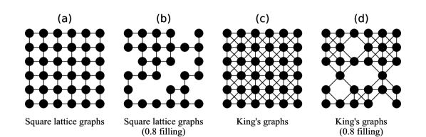
We compute the counting of all independent sets for graphs shown in Figure 2, where vertices are all placed on square lattices of dimensions . The types of graphs include: the square lattice graphs (Figure 2(a)), the square lattice graphs with a filling factor , which means sites are occupied with vertices (Figure 2(b)), the King’s graphs (Figure 2(c)), the King’s graphs with a filling factor (Figure 2(d)), which is the ensemble of graphs used in Ref. [19] to benchmark quantum algorithms on a Rydberg atom array quantum computer.
The number of independent sets for square lattice graphs of size form a well-known integer sequence (OEIS A006506), which is thought as a two-dimensional generalization of the Fibonacci numbers. We computed the integer sequence for and , which is, to the best of our knowledge, not known before. In the computation, we used finite-field algebra for contracting integer tensor networks with arbitrarily high precision.
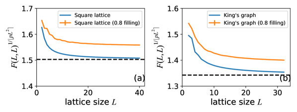
A theoretically interesting number that can be computed using the number of independent sets is the entropy constant, which can describe the thermodynamic properties of hard-core lattice gases at the high-temperature limit. For the square lattice graphs, this number is called the hard square entropy constant (OEIS A085850), which is defined as , where is the number of independent sets of a given lattice dimensions . This quantity arises in statistical mechanics of hard-square lattice gases [5, 51] and is used to understand phase transitions for these systems. This entropy constant is not known to have an exact representation, but it is accurately known in many digits. Similarly, we can define entropy constants for other lattice gases. In Figure 3, we look at how scales as a function of the grid size for all types of graphs shown in Figure 2. Our results match the known results for the non-disordered square lattice and King’s graphs. For disordered square lattice and King’s graphs with a filling factor , we randomly sample 1000 graph instances. To our knowledge, the entropy constants for these disordered graphs have not been studied before. They may be used to study phase transitions for disordered lattices, which are typically much harder to understand. Interestingly, the variations due to different random instances are negligible for this quantity.
9.2 The overlap gap property
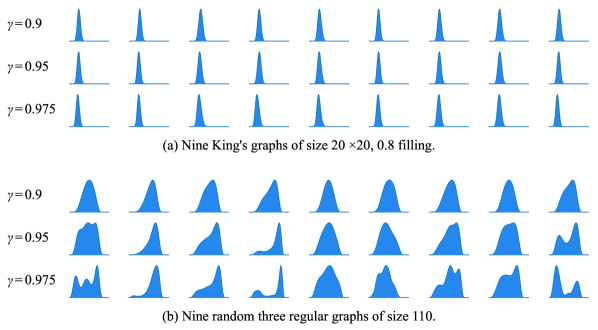
With this tool to enumerate or sample configurations, one can understand the structure of the independent set configuration space, such as the optimization landscape for finding the MISs. One of the known barriers to finding the MIS is the so-called overlap gap property [28, 27]. If the overlap gap property is present, it means every two large independent sets either have a significant intersection or a very small intersection; it implies that large independent sets are clustered together. This clustering property has been used to rigorously prove upper bounds on the performance of local search algorithms [28, 27]. To investigate the overlap gap property, we compute pair-wise Hamming distance distributions of large independent sets as they are good indicators of the presence or absence of overlap gap properties. We inspect two types of graphs that are particularly interesting, the King’s graphs with defects and -regular graphs. It is known that the MIS problem on a general graph can be mapped to the King’s graph with defects [29, 19]. However, it is not clear whether the MIS problem defined on a randomly generated King’s graph with defects can have the overlap gap property. It is known that finding MISs of a -regular graphs has the overlap gap property [53, 26] when both and the graph sizes are large, but, it is not known whether, for small , e.g. for -regular graphs, this statement remains true. We randomly generated instances for each category of King’s graph at filling with dimensions ( vertices) and -regular graphs with vertices. At this problem size, there are too many independent sets to fit into any storage, hence we combine the truncated polynomial and sum-product expression tree to directly sample from the target configuration space. For each instance , we sample pairs of configurations from the independent sets of sizes and show the pair-wise Hamming distance distribution in Figure 4. We observe a clear single peak structure at a fixed distance normalized by the MIS size for the King’s graphs, indicating the absence of the overlap gap property in a random King’s graph at filling. Since the MIS problem on an arbitrary graph can be mapped to a King’s graph at a certain filling, this result is highly nontrivial. It likely implies that the King’s graphs with defects mapped from hard MIS instances have a very small measure in the total defected King’s graph space. In contrast, very different pair-wise Hamming distributions are obtained in Figure 4(b), where we observed the multiple peak structure when the control parameter is big enough. It indicates the existence of disconnected clusters in the configuration space of the MIS problem on -regular graphs. We expect this numerical tool can be used to understand this phenomenon better and to further investigate the graph properties and the geometry of the configuration spaces for a variety of graph instances.
9.3 Analyzing quantum and classical algorithms for Maximum Independent Set
In a recent work, the ability to enumerate configurations and compute independence polynomials was critical in understanding the performance of quantum optimization algorithms for the MIS problem on a Rydberg atom quantum computer [19]. This work focused on exploring King’s graphs with filling. The hardest instances for classical simulated annealing could be accurately predicted from the independence polynomial, which gave information about the density of local minima at different independent set sizes. On the hardest graph instances for simulated annealing studied in the experiment, a high density of local minima were found at independent set sizes of which the algorithm became trapped in instead of finding the optimal solution of size . By enumerating the configurations using techniques described in the present work, we found that simulated annealing randomly explores the independent sets of size until an optimum solution is found. Therefore, the large ratio of local to global minima prevents simulated annealing from efficiently finding an MIS.
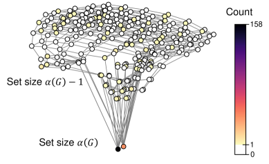
Although the performance of the quantum algorithm is more challenging to understand due to the inherent difficulty in studying quantum systems, the present methods allow one to gain significant insights by visualizing the experimental outputs of a quantum algorithm over the solution space, as shown in Figure 5 for instances with nodes [19]. Here, the structure of the solution space is shown on a graph where each vertex represents a large independent set. Each edge represents a pair of independent sets that differ by a swap operation or a vertex addition to the set, which are the operations naturally present in the effective dynamics at the end of the quantum algorithm. The solution space graph is well-connected by local changes to the spin configurations, has a small diameter, and the degree of each node appears to concentrate. This visualization makes it clear that the quantum algorithm does not appear to return solely local minima with a large Hamming distance from the MISs as suggested for adiabatic algorithms e.g. by Ref. [4] which would appear as a long path on the solution space graph from the sampled local minima to the MIS. Instead, the quantum algorithm samples from local minima across the solution space graph with a wide range of Hamming distances from the MISs. In the case where a large superposition state of local minima is created during the coherent evolution, the quantum algorithm achieves a quadratic speedup over simulated annealing [19]. Looking forward, we expect these tools can be applied to understanding the performance of quantum and classical algorithms on a wide class of NP-hard combinatorial optimization problems.
10 Discussion and conclusion
In this work, we introduced a framework that uses generic tensor networks to compute different solution space properties of a certain class of NP-hard combinatorial optimization problems. Each solution space property is computed using the same tensor network with different tensor element algebra. The different data types introduced in the main text to compute these properties are summarized in the diagram in Figure 1. The class of problems solvable by a tensor network includes but is not limited to maximum independent sets and a variety of other combinatorial problems such as the matching problem, the k-coloring problem, the max-cut problem, the set packing problem, and the set covering problem, as detailed in Appendix B.
Looking ahead, it could be possible to generalize the idea of generic programming to other algorithms that have certain algebraic structures such as those using the inclusion-exclusion principle or subset convolution [25] and explore what new properties can be computed. To this end, dynamic programming [17, 25] approaches could be considered. Dynamic programming is closely related to a tropical tensor network [43]; for example, the Viterbi algorithm for finding the most probable configuration in a hidden Markov model can be interpreted as a matrix product state featured with tropical algebra, and the tropical tensor network in the main text is potentially equivalent to dynamic programming in finding an optimum solution. Since dynamic programming has much broader applications, it would be interesting to extend the ideas from this paper to provide an algebraic interpretation for dynamic programming so that it can be used to compute other solution space properties beyond just finding an optimum solution. It is also possible to extend this idea to other algebras. For example, generic semiring algebra has been used in computational linguistics to compute interesting quantities of a given grammar and string [32].
The source code in the Julia language for this paper can be found in the Github repository [1]. There is a short introduction to this repository as well a gist to show how it works in Appendix J as well. We expect our tool can be used to understand and study many interesting applications of independent sets and beyond. We also hope the toolkit we built, including tensor network contraction order optimization and efficient tropical matrix multiplication, can be helpful to the development of other scientific software.
Acknowledgments
We would like to thank Pan Zhang for sharing his python code for optimizing contraction orders of a tensor network. We acknowledge Sepehr Ebadi and Leo Zhou for coming up with many interesting questions about independent sets and their questions strongly motivated the development of this project. We thank Benjamin Schiffer for providing helpful feedback on the writing of this manuscript. We thank Chris Elord for helping us write the fastest matrix multiplication library for tropical numbers, TropicalGEMM.jl. We thank Jacob Miller for helpful discussions. We would also like to thank a number of open-source software developers, including Roger Luo, Time Besard, Edward Scheinerman, and Katharine Hyatt for actively maintaining their packages and resolving related issues voluntarily. We acknowledge financial support from the DARPA ONISQ program (grant no. W911NF2010021), the Center for Ultracold Atoms, the National Science Foundation, the Vannevar Bush Faculty Fellowship, the U.S. Department of Energy (DE-SC0021013 and DOE Quantum Systems Accelerator Center (contract no. 7568717), the Army Research Office MURI. We acknowledge the computation credits provided by Amazon Web Services for running the benchmarks and case studies. Jinguo Liu acknowledges funding support provided by QuEra Computing Inc. through a sponsored research program.
References
- [1] https://github.com/QuEraComputing/GenericTensorNetworks.jl.
- [2] https://github.com/TensorBFS/TropicalGEMM.jl.
- [3] S. Alikhani and Y. hock Peng, Introduction to domination polynomial of a graph, 2009, https://arxiv.org/abs/0905.2251.
- [4] B. Altshuler, H. Krovi, and J. Roland, Anderson localization makes adiabatic quantum optimization fail, Proceedings of the National Academy of Sciences, 107 (2010), pp. 12446–12450, https://doi.org/10.1073/pnas.1002116107.
- [5] R. J. Baxter, I. G. Enting, and S. K. Tsang, Hard-square lattice gas, Journal of Statistical Physics, 22 (1980), pp. 465–489, https://doi.org/10.1007/BF01012867.
- [6] T. Besard, C. Foket, and B. De Sutter, Effective extensible programming: unleashing julia on gpus, IEEE Transactions on Parallel and Distributed Systems, 30 (2018), pp. 827–841, 10.1109/TPDS.2018.2872064.
- [7] J. Bezanson, S. Karpinski, V. B. Shah, and A. Edelman, Julia: A fast dynamic language for technical computing, 2012, https://arxiv.org/abs/1209.5145.
- [8] J. Biamonte and V. Bergholm, Tensor networks in a nutshell, 2017, https://arxiv.org/abs/1708.00006.
- [9] J. D. Biamonte, J. Morton, and J. Turner, Tensor network contractions for #SAT, Journal of Statistical Physics, 160 (2015), pp. 1389–1404, https://doi.org/10.1007/s10955-015-1276-z, https://doi.org/10.1007%2Fs10955-015-1276-z.
- [10] C. M. Bishop, Pattern Recognition and Machine Learning, Springer, 2006, https://link.springer.com/gp/book/9780387310732.
- [11] M. Bousquet-Mélou, S. Linusson, and E. Nevo, On the independence complex of square grids, Journal of Algebraic combinatorics, 27 (2008), pp. 423–450, https://doi.org/10.1007/s10801-007-0096-x.
- [12] C. Bron and J. Kerbosch, Algorithm 457: finding all cliques of an undirected graph, Communications of the ACM, 16 (1973), pp. 575–577, https://doi.org/10.1145/362342.362367.
- [13] S. Butenko and P. M. Pardalos, Maximum Independent Set and Related Problems, with Applications, PhD thesis, USA, 2003, https://ufdc.ufl.edu/UFE0001011/00001.
- [14] P. Butera and M. Pernici, Sums of permanental minors using grassmann algebra, 2014, https://arxiv.org/abs/1406.5337.
- [15] A. Cichocki, Era of big data processing: A new approach via tensor networks and tensor decompositions, 2014, https://doi.org/10.48550/ARXIV.1403.2048.
- [16] J. I. Cirac, D. Pé rez-García, N. Schuch, and F. Verstraete, Matrix product states and projected entangled pair states: Concepts, symmetries, theorems, Reviews of Modern Physics, 93 (2021), https://doi.org/10.1103/revmodphys.93.045003.
- [17] B. Courcelle, The monadic second-order logic of graphs. i. recognizable sets of finite graphs, Information and computation, 85 (1990), pp. 12–75, https://doi.org/10.1016/0890-5401(90)90043-H.
- [18] J. C. Dyre, Simple liquids’ quasiuniversality and the hard-sphere paradigm, Journal of Physics: Condensed Matter, 28 (2016), p. 323001, https://doi.org/10.1088/0953-8984/28/32/323001.
- [19] S. Ebadi, A. Keesling, M. Cain, T. T. Wang, H. Levine, D. Bluvstein, G. Semeghini, A. Omran, J.-G. Liu, R. Samajdar, X.-Z. Luo, B. Nash, X. Gao, B. Barak, E. Farhi, S. Sachdev, N. Gemelke, L. Zhou, S. Choi, H. Pichler, S.-T. Wang, M. Greiner, V. Vuletić, and M. D. Lukin, Quantum optimization of maximum independent set using rydberg atom arrays, Science, 376 (2022), pp. 1209–1215, https://doi.org/10.1126/science.abo6587, https://www.science.org/doi/abs/10.1126/science.abo6587, https://arxiv.org/abs/https://www.science.org/doi/pdf/10.1126/science.abo6587.
- [20] D. Eppstein, M. Löffler, and D. Strash, Listing all maximal cliques in sparse graphs in near-optimal time, in Algorithms and Computation, O. Cheong, K.-Y. Chwa, and K. Park, eds., Berlin, Heidelberg, 2010, Springer Berlin Heidelberg, pp. 403–414, https://doi.org/10.1007/978-3-642-17517-6_36.
- [21] J. Fairbanks, M. Besanȩon, S. Simon, J. Hoffiman, N. Eubank, and S. Karpinski, Juliagraphs/graphs.jl: an optimized graphs package for the julia programming language, 2021, https://github.com/JuliaGraphs/Graphs.jl/.
- [22] H. C. M. Fernandes, J. J. Arenzon, and Y. Levin, Monte carlo simulations of two-dimensional hard core lattice gases, The Journal of Chemical Physics, 126 (2007), p. 114508, https://doi.org/10.1063/1.2539141.
- [23] G. M. Ferrin, Independence polynomials, (2014), https://scholarcommons.sc.edu/etd/2609/.
- [24] F. V. Fomin and K. Høie, Pathwidth of cubic graphs and exact algorithms, Information Processing Letters, 97 (2006), pp. 191–196, https://doi.org/10.1016/j.ipl.2005.10.012.
- [25] F. V. Fomin and P. Kaski, Exact exponential algorithms, Communications of the ACM, 56 (2013), pp. 80–88, https://doi.org/10.1145/2428556.2428575.
- [26] D. Gamarnik, The overlap gap property: A topological barrier to optimizing over random structures, Proceedings of the National Academy of Sciences, 118 (2021), https://doi.org/10.1073/pnas.2108492118.
- [27] D. Gamarnik and A. Jagannath, The overlap gap property and approximate message passing algorithms for -spin models, 2019, https://arxiv.org/abs/1911.06943.
- [28] D. Gamarnik and M. Sudan, Limits of local algorithms over sparse random graphs, 2013, https://arxiv.org/abs/1304.1831.
- [29] M. R. Garey and D. S. Johnson, The Rectilinear Steiner Tree Problem is -Complete, SIAM Journal on Applied Mathematics, 32 (1977), pp. 826–834, https://doi.org/10.1137/0132071.
- [30] S. Gaspers, D. Kratsch, and M. Liedloff, On independent sets and bicliques in graphs, Algorithmica, 62 (2012), pp. 637–658, https://doi.org/10.1007/s00453-010-9474-1.
- [31] G. H. Golub and C. F. Van Loan, Matrix computations, vol. 3, JHU press, 2013, https://doi.org/10.2307/3621013.
- [32] J. Goodman, Semiring parsing, Computational Linguistics, 25 (1999), pp. 573–606, https://aclanthology.org/J99-4004.pdf.
- [33] J. Gray and S. Kourtis, Hyper-optimized tensor network contraction, Quantum, 5 (2021), p. 410, https://doi.org/10.22331/q-2021-03-15-410.
- [34] C. R. Harris, K. J. Millman, S. J. van der Walt, R. Gommers, P. Virtanen, D. Cournapeau, E. Wieser, J. Taylor, S. Berg, N. J. Smith, R. Kern, M. Picus, S. Hoyer, M. H. van Kerkwijk, M. Brett, A. Haldane, J. Fernández del Río, M. Wiebe, P. Peterson, P. Gérard-Marchant, K. Sheppard, T. Reddy, W. Weckesser, H. Abbasi, C. Gohlke, and T. E. Oliphant, Array programming with NumPy, Nature, 585 (2020), p. 357–362, https://doi.org/10.1038/s41586-020-2649-2.
- [35] N. J. Harvey, P. Srivastava, and J. Vondrák, Computing the independence polynomial: from the tree threshold down to the roots, in Proceedings of the Twenty-Ninth Annual ACM-SIAM Symposium on Discrete Algorithms, SIAM, 2018, pp. 1557–1576, https://doi.org/10.1137/1.9781611975031.102.
- [36] J. Hastad, Clique is hard to approximate within , in Proceedings of 37th Conference on Foundations of Computer Science, IEEE, 1996, pp. 627–636, https://doi.org/10.1007/BF02392825.
- [37] D. S. Johnson, M. Yannakakis, and C. H. Papadimitriou, On generating all maximal independent sets, Information Processing Letters, 27 (1988), pp. 119–123, https://doi.org/10.1016/0020-0190(88)90065-8.
- [38] G. Kalachev, P. Panteleev, and M.-H. Yung, Multi-tensor contraction for xeb verification of quantum circuits, 2021, https://arxiv.org/abs/2108.05665.
- [39] L. R. Kerr, The effect of algebraic structure on the computational complexity of matrix multiplication, tech. report, Cornell University, 1970, https://ecommons.cornell.edu/handle/1813/5934.
- [40] S. Kourtis, C. Chamon, E. Mucciolo, and A. Ruckenstein, Fast counting with tensor networks, SciPost Physics, 7 (2019), https://doi.org/10.21468/scipostphys.7.5.060.
- [41] T.-D. Lee and C.-N. Yang, Statistical theory of equations of state and phase transitions. ii. lattice gas and ising model, Physical Review, 87 (1952), p. 410, https://doi.org/10.1103/PhysRev.87.410.
- [42] V. E. Levit and E. Mandrescu, The independence polynomial of a graph at -1, 2009, https://arxiv.org/abs/0904.4819.
- [43] J.-G. Liu, L. Wang, and P. Zhang, Tropical tensor network for ground states of spin glasses, Physical Review Letters, 126 (2021), https://doi.org/10.1103/physrevlett.126.090506.
- [44] D. Maclagan and B. Sturmfels, Introduction to tropical geometry, vol. 161, American Mathematical Soc., 2015, http://www.cs.technion.ac.il/~janos/COURSES/238900-13/Tropical/MaclaganSturmfels.pdf.
- [45] F. Manne and S. Sharmin, Efficient counting of maximal independent sets in sparse graphs, in International Symposium on Experimental Algorithms, Springer, 2013, pp. 103–114, https://doi.org/10.1007/978-3-642-38527-8_11.
- [46] I. L. Markov and Y. Shi, Simulating quantum computation by contracting tensor networks, SIAM Journal on Computing, 38 (2008), p. 963–981, https://doi.org/10.1137/050644756.
- [47] C. Moore and S. Mertens, The nature of computation, OUP Oxford, 2011, https://doi.org/10.1093/acprof:oso/9780199233212.001.0001.
- [48] R. Orús, A practical introduction to tensor networks: Matrix product states and projected entangled pair states, Annals of Physics, 349 (2014), pp. 117–158, https://doi.org/10.1016/j.aop.2014.06.013.
- [49] I. V. Oseledets, Tensor-train decomposition, SIAM Journal on Scientific Computing, 33 (2011), pp. 2295–2317, https://doi.org/10.1137/090752286.
- [50] F. Pan and P. Zhang, Simulating the sycamore quantum supremacy circuits, 2021, https://arxiv.org/abs/2103.03074.
- [51] P. A. Pearce and K. A. Seaton, A classical theory of hard squares, Journal of Statistical Physics, 53 (1988), pp. 1061–1072, https://doi.org/10.1007/BF01023857.
- [52] H. Pichler, S.-T. Wang, L. Zhou, S. Choi, and M. D. Lukin, Quantum optimization for maximum independent set using rydberg atom arrays, 2018, https://doi.org/10.48550/ARXIV.1808.10816, https://arxiv.org/abs/1808.10816.
- [53] M. Rahman and B. Virág, Local algorithms for independent sets are half-optimal, The Annals of Probability, 45 (2017), https://doi.org/10.1214/16-aop1094.
- [54] J. M. Robson, Algorithms for maximum independent sets, Journal of Algorithms, 7 (1986), pp. 425–440, https://doi.org/10.1016/0196-6774(86)90032-5.
- [55] A. Schönhage and V. Strassen, Schnelle multiplikation grosser zahlen, Computing, 7 (1971), pp. 281–292, https://doi.org/10.1007/BF02242355.
- [56] Y. Shitov, The complexity of tropical matrix factorization, Advances in Mathematics, 254 (2014), pp. 138–156, https://doi.org/10.1016/j.aim.2013.12.013.
- [57] A. A. Stepanov and D. E. Rose, From mathematics to generic programming, Pearson Education, 2014, https://www.fm2gp.com/.
- [58] R. E. Tarjan and A. E. Trojanowski, Finding a maximum independent set, SIAM Journal on Computing, 6 (1977), pp. 537–546, https://doi.org/10.1137/0206038.
- [59] Q. Wu and J.-K. Hao, A review on algorithms for maximum clique problems, European Journal of Operational Research, 242 (2015), pp. 693–709, https://doi.org/10.1016/j.ejor.2014.09.064.
- [60] Y.-Z. Xu, C. H. Yeung, H.-J. Zhou, and D. Saad, Entropy inflection and invisible low-energy states: Defensive alliance example, Physical Review Letters, 121 (2018), https://doi.org/10.1103/physrevlett.121.210602.
- [61] C.-N. Yang and T.-D. Lee, Statistical theory of equations of state and phase transitions. i. theory of condensation, Physical Review, 87 (1952), p. 404, https://doi.org/10.1103/PhysRev.87.404.
Appendix A An alternative way to construct the tensor network
Let us characterize the independent set problem on graph as an energy model with two parts
| (29) |
where is a spin on vertex and is an onsite energy term associated with it. The first part corresponds to the negative independent set size and the second part describes the independence constraint, which corresponds to the Rydberg blockade [52, 19] in cold atom arrays or the repulsive force in hardcore lattice models [18, 22]. The partition function is defined as
| (30) |
where is the set of independent sets of graph , is the absolute value of the minimum energy (maximum independent set size), is the number of spin configurations with energy (independent sets of size ). The partition function can be expressed as a tensor network by placing a vertex tensor on each spin
| (31) |
and an edge tensor on each bond
| (32) |
where the in the edge tensor comes from in the second term of Equation 29, which is the independence constraint. By letting , we get the tensor network for computing the independence polynomial as described by Equation 5 and Equation 6. If we further let , the second line of Equation 30 is equivalent to the independence polynomial.
Appendix B Hard problems and tensor networks
B.1 Maximal independent sets and maximal cliques
In this section, we focus the discussion on the maximal independent sets problem since finding maximal cliques of a graph is equivalent to finding the maximal independent sets of its complement. Let be a graph; we denote the neighborhood of a vertex as . A maximal independent set is an independent set such that no satisfies , i.e. an independent set that cannot become a larger one by adding a new vertex. The corresponding tensor network can be specified as
| (33) |
where we defined a tensor for each and its neighborhood as
| (34) |
Here, is the th vertex in and is the degree of vertex . If , then none of its neighbours can be a member of by the independence constraint, contributing a factor . If , then at least on of its neighbors must be in by the maximal constraint, contributing a unit factor. For a degree 2 vertex , the tensor has the following form
| (35) |
Theorem B.1.
The tensor network representation of a maximal independent set problem on a graph (Equation 33) can be contracted in number of additions and multiplications, where is the maximum degree of vertices in .
Proof B.2.
The prefactor comes from the number of tensors, while the contraction complexity of pair-wise tensor contraction is closely related to the treewidth of the line graph of its hypergraph representation . In the following, we will show this quantity is upper bounded by times the treewidth of . In the line graph , a tensor corresponds to a clique over . In the following, we will show given an optimal tree decomposition of , it is always possible to include all cliques into the bags by increasing the bag size by a factor . Let be a vertex and be its neighborhood; we first arbitrarily pick an edge , then by the definition of tree decomposition, we can find a bag containing this edge, and lastly we include all into this bag. Hence the maximum tensor rank during contraction is upper bounded by , proving the theorem.
Let us consider the graph in Example 4.4. The corresponding tensor network structure for computing the maximal independent polynomial has the following hypergraph representation.
{tikzpicture}[ dot/.style = circle, fill, minimum size=#1, inner sep=0pt, outer sep=0pt, dot/.default = 6pt ] ; \foreach\x/\y/in 0/0/a, 1/0/b, 2/0/c, 3/0/d, 4/0/e \node[color=black] at (\x*1.0+0,\y) () ; \foreach\x//i͡n 0/A/, 1/B/, 2/C/, 3/D/, 4/E/ \node[color=white,fill=black,dot=0.4cm] at (\x*1.0+0,1.5) () -; \draw[cyan,thick] (a) – (A); \draw[cyan,thick] (a) – (B); \draw[cyan,thick] (a) – (C); \draw[blue,thick] (b) – (B); \draw[blue,thick] (b) – (A); \draw[blue,thick] (b) – (C); \draw[blue,thick] (b) – (D); \draw[red,thick] (c) – (C); \draw[red,thick] (c) – (A); \draw[red,thick] (c) – (B); \draw[red,thick] (c) – (D); \draw[green,thick] (d) – (D); \draw[green,thick] (d) – (B); \draw[green,thick] (d) – (C); \draw[green,thick] (d) – (E); \draw[orange,thick] (e) – (E); \draw[orange,thick] (e) – (D);
By contracting this tensor network with generic element types, we can compute the maximal independent set properties such as the maximal independence polynomial and the enumeration of maximal independent sets. The maximal independence polynomial is defined as
| (36) |
where is the number of maximal independent sets of size . Comparing with the independence polynomial in Equation 9, we have and . counts the total number of maximal independent sets [30, 45]; to our knowledge, the best algorithm has a time complexity [30].
The benchmark of computing the maximal independent set properties on -regular graphs is shown in Appendix F.
B.2 Matching problem
A -matching in a graph is a set of edges that no two of which have a vertex in common. We map an edge to a degree of freedom in a tensor network, where means an edge is in the set and otherwise. The tensor network representation for the matching problem can be specified as
| (37) |
where for each , we define a vertex tensor over its neighborhood as
| (38) |
and for each bond , we define a rank one tensor as
| (39) |
Here, is the th vertex in and is the degree of vertex ; a label is equivalent to . tensor specifies the constraint that a vertex cannot be shared by two edges in the edge set, and an edge tensor carries the weights.
Theorem B.3.
The tensor network representation of a matching problem on graph (Equation 37) can be contracted in number of additions and multiplications, where is the line graph of .
Proof B.4.
To contract the tensor network, we first absorb edges tensors into the vertex tensors, which does not increase computational complexity. After this, the resulting tensor network is isomorphic to . Hence the contraction complexity is .
Let ; the tensor network contraction corresponds to the matching polynomial
| (40) |
where is the size of an edge set, and a coefficient is the number of -matchings.
B.3 Vertex coloring
Let be a graph. A vertex coloring is an assignment of colors to each vertex such that no edge connects two identically colored vertices. In a -coloring problem, the number of colors is limited to less or equal to . Let us use the 3-coloring problem as an example to show how to reduce it to tensor contractions. We first map a vertex to a degree of freedom . The tensor network for the vertex coloring problem can be specified as
| (41) |
where for each vertex , we define a tensor labelled by
| (42) |
and for each edge , we define a tensor labelled by as
| (43) |
where subscripts , and are for labeling the color configurations. tensors are for specifying the coloring constraints and tensors are for labeling the solutions.
Theorem B.5.
The tensor network representation of a K-coloring problem on a graph (Equation 41) can be contracted in number of additions and multiplications.
The proof is similar to that for Theorem 4.2 except the dimension of each degree of freedom is . Let and ; we then have a graph polynomial, in which the -th coefficient is the number of coloring that bonds satisfy constraints. If a graph is colorable, the maximum order of this polynomial should be equal to the number of edges in this graph. Similarly, one can define an edge coloring problem by defining the tensor network on the line graph of .
B.4 Cutting problem
In graph theory, a cut is a partition of the vertices of a graph into two disjoint subsets, which is also known as the spin-glass problem in statistical physics. Let be a graph. We associate a weight to each . To reduce the cutting problem on to the contraction of a tensor network, we first define a Boolean degree of freedom for each vertex . The tensor network representation for the cutting problem can be specified as
| (44) |
where for each edge , we define an edge matrix labelled by as
| (45) |
Here, variables and are for a cut on this edge or a domain wall in a spin glass problem.
Theorem B.6.
The tensor network representation of a cuting problem on a graph (Equation 44) can be contracted in number of additions and multiplications.
The proof is similar to that for Theorem 4.2. Let ; we have a graph polynomial similar to the previous ones, in which the th coefficient is two times the number of cut configurations that have size (i.e. cutting edges).
B.5 Dominating Set
In graph theory, a dominating set for a graph is a subset such that every vertex not in is adjacent to at least one member of . To reduce this problem to the contraction of a tensor network, we first map a vertex to a Boolean degree of freedom . The tensor network for the dominating set problem can be specified as
| (46) |
where for each vertex , we define a tensor on its closed neighborhood as
| (47) |
Here, is the weight associated with the vertex , is the th vertex in and is the degree of vertex . This tensor implies a configuration having a closed neighborhood of not in () cannot be a dominating set. Otherwise, if is in , this tensor contributes a multiplicative factor to the output.
Theorem B.7.
The tensor network representation of a dominating set problem on a graph (Equation 46) can be contracted in number of additions and multiplications.
The proof is similar to that for Theorem B.1. The graph polynomial for the dominating set problem is known as the domination polynomial [3]
| (48) |
where is the number of dominating sets of size .
B.6 Boolean satisfiability Problem
The Boolean satisfiability problem is the problem of determining if there exists an assignment that satisfies a given Boolean formula. One can specify a satisfiable problem in the conjunctive normal form (CNF), i.e. a conjunction of clauses (or disjunctions of Boolean literals). Given the alphabet of Boolean variables and its negation , a CNF can be formally defined as
| (49) |
where is the number of clauses, is the th clause and is the th literal in it. The standard tensor network can be used to study the counting version of the satisfiability problem [9], while in the following, we will show a generic reduction from the problem of solving a CNF to a tensor network contraction for solving more solution space properties. We first map each Boolean literal to a Boolean degree of freedom . stands for variable having value false while stands for having value true. The tensor network can be specified as
| (50) |
where a tensor defined on literal is
| (51) |
and a tensor defined on the clause is
| (52) |
where is the th literal in with its negation sign removed and is the number of boolean variables in it; is the weight associated with clause .
Theorem B.8.
The tensor network representation of a CNF (Equation 50) can be contracted in number of additions and multiplications, where is the number of clauses, is a hypergraph constructed by mapping a variable to a vertex and the th clause to a hyperedge connecting .
This can be proved by showing the hypergraph is the line graph of . Let and ; one can get a polynomial, in which the -th coefficient gives the number of assignments that clauses are satisfied.
B.7 Set packing
Suppose one has a finite set and a list of subsets of , denoted as . Then, the set packing problem asks if some subsets in are pairwise disjoint. It is the hypergraph generalization of the independent set problem, where a set corresponds to a vertex and an element corresponds to a hyperedge. The generic tensor network for the set packing problem also has a similar form as that for the independent set problem
| (53) |
where for each , we have the constraints over sets, , that containing it as
| (54) |
and the vertex tensor for each
| (55) |
where is the th element in and is the number of elements in .
Theorem B.9.
The tensor network representation of a set packing problem (Equation 53) can be contracted in number of additions and multiplications, where is the number of sets, is a hypergraph constructed by mapping a set to a vertex and element to a hyperedge connecting sets, , that containing it.
This can be proved by showing the hypergraph is the line graph of .
B.8 Set covering
Suppose one has a finite set and a list of subsets of , denoted as . The set covering problem aims to find the minimum number of sets in that incorporate (cover) all of elements in . To get the generic tensor network representation, we first map a set to a Boolean degree of freedom . Then the tensor network representation for the set covering problem can be specified as
| (56) |
where for each , we define a parameterized rank-one tensor indexed by it as
| (57) |
where is a generic typed variable associated with and is a positive integer as the weight. For each element , we can define a constraint over all containing this element, i.e. , as
| (58) |
where is the th element in and is the number of elements in . If a subset of does not include any sets containing element , then the corresponding entry is zero.
Theorem B.10.
The tensor network representation of a set covering problem (Equation 56) can be contracted in number of additions and multiplications, where is the number of sets, is a hypergraph constructed by mapping a set to a vertex and element to a hyperedge connecting sets , that containing it.
This can be proved by showing the hypergraph is the line graph of .
Appendix C Bounding the MIS enumeration space
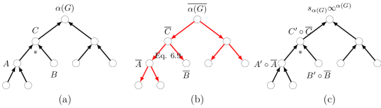
When using the algebra in Equation 21: P1+SN to enumerate all MISs, the program often stores significantly more intermediate configurations than necessary. To reduce the space overhead, we will show how to bound the searching space using the MIS size . The bounded contraction consists of three stages as shown in Figure 6. (a) We first compute the value of with tropical algebra and cache all intermediate tensors. (b) Then, we compute a Boolean mask for each cached tensor, where we use a Boolean true to represent a tensor element having a contribution to the MIS and Boolean false otherwise. (c) Finally, we perform masked tensor network contraction (i.e. discarding elements masked false) using the element type with the algebra in Equation 21: P1+SN to obtain all MIS configurations. The crucial part is computing the masks in step (b). Note that these masks correspond to tensor elements with non-zero gradients to the MIS size; we can compute these masks by back-propagating the gradients. To derive the back-propagation rule for tropical tensor contraction, we first reduce the problem to finding the back-propagation rule of a tropical matrix multiplication . Since with tropical algebra, we have the following inequality
| (59) |
Here on tropical numbers are the same as the real-number algebra. The equality holds for some , which means and have contributions to . Intuitively, one can use this relation to identify elements with nonzero gradients in and , but if doing this directly, one loses the advantage of using BLAS libraries [2] for high performance. Since , one can move to the right hand side of the inequality:
| (60) |
where ∘-1 is the element-wise multiplicative inverse on tropical algebra (which is the additive inverse on real numbers). The inequality still holds if we take the minimum over :
| (61) |
On the right-hand side, we transform the operation into a tropical matrix multiplication so that we can utilize the fast tropical BLAS routines [2]. Again, the equality holds if and only if the element has a contribution to (i.e. having a non-zero gradient). Let the gradient mask for be ; the back-propagation rule for gradient masks reads
| (62) |
where is the Dirac delta function that returns one if two arguments have the same value and zero otherwise, is the element-wise product, Boolean false is treated as the tropical number , and Boolean true is treated as the tropical number . This rule defined on matrix multiplication can be easily generalized to tensor contraction by replacing the matrix multiplication between and by a tensor contraction. With the above method, one can significantly reduce the space needed to store the intermediate configurations by setting the tensor elements masked false to zero during contraction.
Appendix D The fitting approach to computing the independence polynomial
In this section, we propose to find the independence polynomial by fitting random pairs of and . One can then compute the independence polynomial coefficients by solving the linear equation:
| (63) |
Unlike using the polynomial numbers in Equation 10: PN, the fitting approach does not have the linear overhead in space. However, since the independence polynomial coefficients can have a huge order-of-magnitude range, the round-off errors can be larger than the value itself when using floating-point numbers in computation. To avoid using the arbitrary precision number that can be very slow and is incompatible with GPU devices, we introduce the following finite-field algebra approach:
| (64: GF) |
Regarding the finite-field algebra, we have the following observations:
-
1.
One can use Gaussian elimination [31] to solve the linear equation Equation 63 since it is a generic algorithm that works for any elements with field algebra. The multiplicative inverse of a finite-field algebra can be computed with the extended Euclidean algorithm.
-
2.
Given the remainders of a larger unknown integer over a set of co-prime integers , can be computed using the Chinese remainder theorem. With this, one can infer big integers from small integers.
With these observations, we develop Algorithm 1 to compute the independence polynomial exactly without introducing space overheads. The algorithm iterates over a sequence of large prime numbers until convergence. In each iteration, we choose a large prime number , and contract the tensor networks to evaluate the polynomial for each variable on and denote the outputs as . Then we solve Equation 63 using Gaussian elimination on to find the coefficient modulo , . As the last step of each iteration, we apply the Chinese remainder theorem to update to , where is a product of all prime numbers chosen in previous iterations. If this number does not change compared with the previous iteration, it indicates the convergence of the result and the program terminates. All computations are done with integers of fixed-width except the last step of applying the Chinese remainder theorem, where we use arbitrary precision integers to represent the counting.
Alternatively, one can use a faster but less accurate Fourier transformation based method to fit this polynomial, which is detailed and benchmarked in Appendix F.
Appendix E Integer sequence formed by the number of independent sets
We computed the number of independent sets on square lattices and King’s graphs with our generic tensor network contraction algorithm on GPUs. The tensor element type is the finite-field algebra so that we can reach an arbitrary precision. We also computed the independence polynomial for these lattices up to size in our GitHub repository.
| square lattice graphs | |
| 616 412 251 028 728 207 385 738 562 656 236 093 713 609 747 387 533 907 560 081 990 229 746 115 948 572 583 817 557 035 128 726 922 565 913 748 716 778 414 190 432 479 964 245 067 083 441 583 742 870 993 696 157 129 887 194 203 643 048 435 362 875 885 498 554 979 326 352 127 528 330 481 118 313 702 375 541 902 300 956 879 563 063 343 972 979 | |
| 29 855 612 447 544 274 159 031 389 813 027 239 335 497 014 990 491 494 036 487 199 167 155 042 005 286 230 480 609 472 592 158 583 920 411 213 748 368 073 011 775 053 878 033 685 239 323 444 700 725 664 632 236 525 923 258 394 737 964 155 747 730 125 966 370 906 864 022 395 459 136 352 378 231 301 643 917 282 836 792 261 715 266 731 741 625 623 207 330 411 607 |
Appendix F Performance benchmarks
We run a single thread benchmark on central processing units (CPU) Intel(R) Xeon(R) CPU E5-2686 v4 @ 2.30GHz, and its CUDA version on a GPU Tesla V100-SXM2 16G. The results are summarized in Figure 7. The graphs in all benchmarks are random three-regular graphs, which have treewidth that is asymptotically smaller than [24]. In this benchmark, we do not include traditional algorithms for finding the MIS sizes such as branching [58, 54] or dynamic programming [17, 25]. To the best of our knowledge, these algorithms are not suitable for computing most of the solution space properties mentioned in this paper. The main goal of this section is to show the relative computation time for calculating different solution space properties.
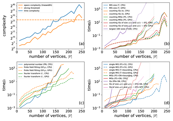
Figure 7(a) shows the time and space complexity of tensor network contraction for different graph sizes. The contraction order is obtained using the local search algorithm in Ref. [38]. If we assume our contraction-order finding program has found the optimal treewidth, which is very likely to be true, the space complexity is the same as the treewidth of the problem graph. Slicing technique [38] has been used for graphs with space complexity greater than (above the yellow dashed line) to fit the computation into a 16GB memory. One can see that all the computation times in Figure 7 (b), (c), and (d) have a strong correlation with the predicted time and space complexity. While in panel (d), the computation time of configuration enumeration and sum-product expression tree generation also strongly correlates with other factors such as the configuration space size. Among these benchmarks, computational tasks with data types real numbers, complex numbers, or tropical numbers (CPU only) can utilize fast basic linear algebra subprograms (BLAS) functions. These tasks usually compute much faster than ones with other element types in the same category. Immutable data types with no reference to other values can be compiled to GPU devices that run much faster than CPUs in all cases when the problem scale is big enough. These data types do not include those defined in Equation 10: PN, Equation 19: SN, Equation 27: T and Equation 25: EXPR or a data type containing them as a part. In Figure 7(c), one can see the Fourier transformation-based method is the fastest in computing the independence polynomial, but it may suffer from round-off errors (Appendix H). The finite field (GF) approach is the only method that does not have round-off errors and can be run on a GPU. In Figure 7(d), one can see the technique to bound the enumeration space in Appendix C improves the performance for more than one order of magnitude in enumerating the MISs. The bounding technique can also reduce the memory usage significantly, without which the largest computable graph size is only on a device with 32GB main memory.
We show the benchmark of computing the maximal independent set properties on -regular graphs in Figure 8, including a comparison to the Bron-Kerbosch algorithm from Julia package Graphs [21]. Figure 8(a) shows the space and time complexities of tensor contraction, which are typically larger than those for the independent set problem. In Figure 8(b), one can see counting maximal independent sets are much more efficient than enumerating them, while our generic tensor network approach runs slightly faster than the Bron-Kerbosch approach in enumerating all maximal independent sets.
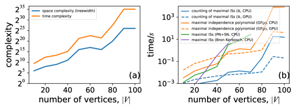
Appendix G An example of increased contraction complexity for the standard tensor network notation
In the standard Einstein’s notation for tensor networks in physics, each index appears precisely twice: either both are in input tensors (which will be summed over) or one is in an input tensor and another in the output tensor. Hence a tensor network can be represented as an open simple graph, where an input tensor is mapped to a vertex, a label shared by two input tensors is mapped to an edge and a label that appears in the output tensor is mapped to an open edge. A standard tensor network notation is equivalent to the generalized tensor network in representation power. A generalized tensor network can be converted to a standard one by adding a tensors at each hyperedge, where a tensor of rank is defined as
| (65) |
In the following example, we will show this conversion might increase the contraction complexity of a tensor network.
Let us consider the following King’s graph.
{tikzpicture} \foreach\xin 1,…,5 \foreach\yin 1,…,5 \filldraw[fill=black] (\x,\y) circle [radius=0.2]; \foreach\xin 1,…,5 \foreach\yin 1,…,4 \draw[black,thick] (\x,\y) – (\x,\y+1); \draw[black,thick] (\y,\x) – (\y+1,\x); \foreach\xin 1,…,4 \foreach\yin 1,…,4 \draw[black,thick] (\x,\y) – (\x+1,\y+1); \draw[black,thick] (\y+1,\x) – (\y,\x+1);
The generalized tensor network for solving the MIS problem on this graph has the following hypergraph representation, where we use different colors to distinguish different hyperedges.
{tikzpicture} \pgfmathsetseed2 \foreach[evaluate= =0.1+0.5*Mod(\x,2)] \xin 1,…,5 \foreach[evaluate=\cg=0.1+0.3*Mod(\y,2); \cy=0.5-0.5*Mod(\y,2)] \yin 1,…,5
Vertex tensors are not shown here because they can be absorbed into an edge tensor and hence do not change the contraction complexity. If we contract this tensor network in the column-wise order, the maximum intermediate tensor has rank , which can be seen by counting the number of colors at the cut.
By adding tensors to hyperedges, we have the standard tensor network represented as the following simple graph.
{tikzpicture} \foreach\xin 1,…,5 \foreach\yin 1,…,5 \filldraw[fill=black] (\x,\y) circle [radius=0.08]; \foreach\xin 1,…,5 \foreach\yin 1,…,4 \filldraw[fill=black] (\x,\y+0.5) circle [radius=0.08]; \filldraw[fill=black] (\y+0.5,\x) circle [radius=0.08]; \draw[black,thick] (\x,\y) – (\x,\y+1); \draw[black,thick] (\y,\x) – (\y+1,\x); \foreach\xin 1,…,4 \foreach\yin 1,…,4 \filldraw[fill=black] (\x+0.3,\y+0.3) circle [radius=0.08]; \filldraw[fill=black] (\y+0.3,\x+0.7) circle [radius=0.08]; \draw[black,thick] (\x,\y) – (\x+1,\y+1); \draw[black,thick] (\y+1,\x) – (\y,\x+1); \tikzsetdecoration=snake,amplitude=.4mm,segment length=2mm, post length=0mm,pre length=0mm \draw[decorate] (2.7, 0.5) – (2.7, 5.5);
In this diagram, the additional tensors can have ranks up to . If we still contract this tensor network in a column-wise order, the maximum intermediate tensor has rank , i.e. the space complexity is , which has a larger complexity than using the generalized tensor network notation.
Appendix H The discrete Fourier transform approach to computing the independence polynomial
In Appendix D in the main text, we show that the independence polynomial can be obtained by solving the linear equation Equation 63 using the finite field algebra. One drawback of using finite field algebra is that its matrix multiplication is less computationally efficient compared with floating-point matrix multiplication. Here, we show an alternative method with standard number types but with controllable round-off errors. Instead of choosing as random numbers, we can choose them such that they form a geometric sequence in the complex domain , where and . The linear equation thus becomes
| (66) |
Let us rearrange the coefficients to , the matrix on the left side becomes the discrete Fourier transform matrix. Thus, we can obtain the coefficients by inverse Fourier transform , where . By choosing different , one can obtain better precision for small by choosing or large by choosing .
Appendix I Computing maximum sum combination
Given two sets and of the same size . It is known that the maximum sum combination of and can be computed in time . The standard approach to solve the sum combination problem requires storing the variables in a heap — a highly dynamic binary tree structure that can be much slower to manipulate than arrays. In the following, we show an algorithm with roughly the same complexity but does not need a heap. This algorithm first sorts both and and then uses the bisection to find the -th largest value in the sum combination. The key point is we can count the number of entries greater than a specific value in the sum combination of and in linear time. As long as the data range is not exponentially large, the bisection can be done in steps, giving the time complexity . We summarize the algorithm as in Algorithm 2.
In this algorithm, function collect_geq is similar the count_geq except the counting is replace by collecting the items to a set. Inside the function count_geq, variable monotoneously increase while monotoneously decrease in each iteration and the total number of iterations is upper bounded by . Here for simplicity, we do not handle the special element in and and the potential degeneracy in the sums. It is nevertheless important to handle them properly in a practical implementation.
Appendix J Technical guides
This appendix covers some technical guides for efficiency, including an introduction to an open-source package GenericTensorNetworks [1] implementing the algorithms in this paper and the gist about how this package is implemented. One can install GenericTensorNetworks in a Julia REPL, by first typing ] to enter the pkg> mode and then typing
followed by an <ENTER> key. To use it for solving solution space properties, just go back to the normal mode (type <BACKSPACE>) and type
Here the main function solve takes three inputs: the problem instance of type IndependentSet, the property instance of type GraphPolynomial and an optional key word argument usecuda to decide to use GPU or not. If one wants to use GPU to accelerate the computation, “using CUDA” must be uncommented. The problem instance takes four arguments to initialize: the only positional argument is the graph instance one wants to solve, the keyword argument optimizer is for specifying the tensor network optimization algorithm, the keyword argument weights is for specifying the weights of vertices as either a vector or NoWeight(), and the keyword argument openvertices is for specifying the degrees of freedom not summed over. Here, we use the TreeSA method as the tensor network optimizer, and leave weights and openvertices as default values. The TreeSA algorithm, which was invented in Ref. [38], performs the best in most of our applications. The first execution of this function will be a bit slow due to Julia’s just-in-time compilation. After that, the subsequent runs will be faster. The following diagram lists possible combinations of input arguments, where functions in the Graph are mainly defined in the package Graphs, and the rest can be found in GenericTensorNetworks.
![[Uncaptioned image]](/html/2205.03718/assets/x8.png)
The code we will show below is a gist of how the above package was implemented, which is mainly for pedagogical purpose. It covers most of the topics in the paper without caring much about performance. It is worth mentioning that this project depends on multiple open source packages in the Julia ecosystem:
- OMEinsum and OMEinsumContractionOrders
- TropicalNumbers and TropicalGEMM
-
are packages providing tropical number and efficient tropical matrix multiplication.
- Graphs
-
is a foundational package for graph manipulation in the Julia community.
- Polynomials
-
is a package providing polynomial algebra and polynomial fitting.
- Mods and the Primes
-
package providing finite field algebra and prime number manipulation.
They can be installed in a similar way to GenericTensorNetworks. After installing the required packages, one can open a Julia REPL, and copy-paste the following code snippet into it.