High-Resolution Quantum Cascade Laser Dual-Comb Spectroscopy in the Mid-Infrared with Absolute Frequency Referencing

I Abstract

Quantum cascade laser (QCL) frequency combs Hugi et al. (2012) have revolutionized mid-infrared (MIR) spectroscopy by their high brightness and fast temporal resolution Klocke et al. (2018), and are a promising technology for fully-integrated and cost-effective sensors Schwarz et al. (2014). As for other integrated comb sources such as micro-combs Kippenberg et al. (2018) and interband cascade laser Bagheri et al. (2018), QCLs have a comb spacing of several GHz, which is adequate for measurements of wide absorbing structures, typically found in liquid or solid samples Klocke et al. (2018). However, high-resolution gas-phase spectra require spectral interleaving and frequency calibration Kuse et al. (2021); Gianella et al. (2022); Lepère et al. (2022). We developed a frequency calibration scheme for fast interleaved measurements with combs featuring multi-GHz spacing. We then demonstrate dual-comb spectroscopy with 600 kHz accuracy in single-shot 54-ms measurements over 40 cm^-1 using two QCLs at 7.8 $\mathrm{\mu}$m. This work is an important contribution towards fast fingerprinting of complex molecular mixtures in the MIR Gianella et al. (2020). Moreover, the calibration scheme could be used with micro-combs for spectroscopy and ranging, both in comb-swept Kuse et al. (2021); Riemensberger et al. (2020) and comb-calibrated setups Del’Haye et al. (2009).

II Main

Over the last two decades, dual-comb spectroscopy Coddington et al. (2016) has developed into a powerful tool for applications requiring fast temporal resolution, high spectral accuracy, and broad spectral coverage. It has enabled difficult or previously impossible measurements, such as multi-species trace gas detection in open-path Giorgetta et al. (2021), monitoring of irreversible processes with micro-second resolution Klocke et al. (2018), hyperspectral 3D imaging Vicentini et al. (2021), and fast determination of isotope ratios of multiple species Parriaux et al. (2022). Moreover, photonic chip integrated comb sources such as micro-combs Kippenberg et al. (2018), quantum cascade lasers (QCL) Hugi et al. (2012), and interband cascade lasers Bagheri et al. (2018), are potential game-changers, by enabling mass-producible integrated gas sensors for demanding fields, such as health, security, environment, and industrial process monitoring.

However, these integrated comb sources, due to their small size, have large (compared to fiber mode-locked lasers) repetition rates, $f_{\mathrm{rep}}$, on the order of 10 GHz or higher. The large $f_{\mathrm{rep}}$, while allowing a high temporal resolution, leads to a sparse spectrum, where narrow molecular absorption are potentially lost between the comb teeth.

This limitation is not unique to dual-comb spectroscopy or to integrated comb sources, and has been addressed by interleaving many (up to many thousands) offset spectra, where $f_{\mathrm{rep}}$ and/or the offset frequency, $f_{\mathrm{o}}$, are tuned in steps Villares et al. (2014); Muraviev et al. (2020); Luo (2020); Hjältén et al. (2021); Lepère et al. (2022) or continuously Gianella et al. (2020); Kuse et al. (2021).

Step-tuning of referenced combs typically consists in stepping the repetition rate by 10s of Hz with dwell times on the order of seconds or more adapted to the measurement. Thus, the full interleaved spectrum is acquired in 10s or 100s of seconds and the frequency accuracy is that of the static comb Muraviev et al. (2020); Hjältén et al. (2021). We note that step-tuning was also used with free running mid-infrared (MIR) QCLs, where a full spectrum was obtained in 1200 s with an accuracy better than 12 MHz Lepère et al. (2022). Continuous sweeps yield faster measurements with higher spectral point density. However, they require an adapted frequency calibration scheme. The endless frequency comb was proposed by Benkler et al. Benkler et al. (2013), but it is not convenient in the MIR as it requires electro-optic components and pulsed emission. Alternatively, the use of an unbalanced Mach-Zehnder interferometer provided frequency scales with 10-MHz level precision for NIR micro-combs Kuse et al. (2021) and MIR QCLs Gianella et al. (2022), with sweep times of 50 $\mathrm{\mu s}$ and 30 ms respectively.

In this work, we present a method to calibrate fast continuous sweeps of multi-GHz frequency combs with sub-MHz accuracy, which can be applied independently of the wavelength range. We thus demonstrate a QCL-based MIR dual comb spectrometer with a unique combination of fast acquisition, high frequency accuracy, and high spectral point density.

As a proof of concept, we measure 43 transitions of the $\nu_{1}$ ro-vibrational band of $\mathrm{N_{2}O}$ and 64 transitions belonging to the $\nu_{4}$ band of $\mathrm{CH_{4}}$. With the former measurement, we characterize the accuracy of the computed frequency scale and assess the precision of the measurement at varying scanning speeds. The latter measurement serves to improve the literature accuracy of the transition frequencies of $\mathrm{CH_{4}}$, independently of two recent works Lepère et al. (2022); Germann et al. (2022).

Rapid scanning and high accuracy are critical features for fingerprinting of complex molecular mixtures and parallel frequency modulated lidar Riemensberger et al. (2020). Accordingly, we trust that our enhanced method for frequency axis calibration is a highly valuable asset for ranging and MIR sensing.

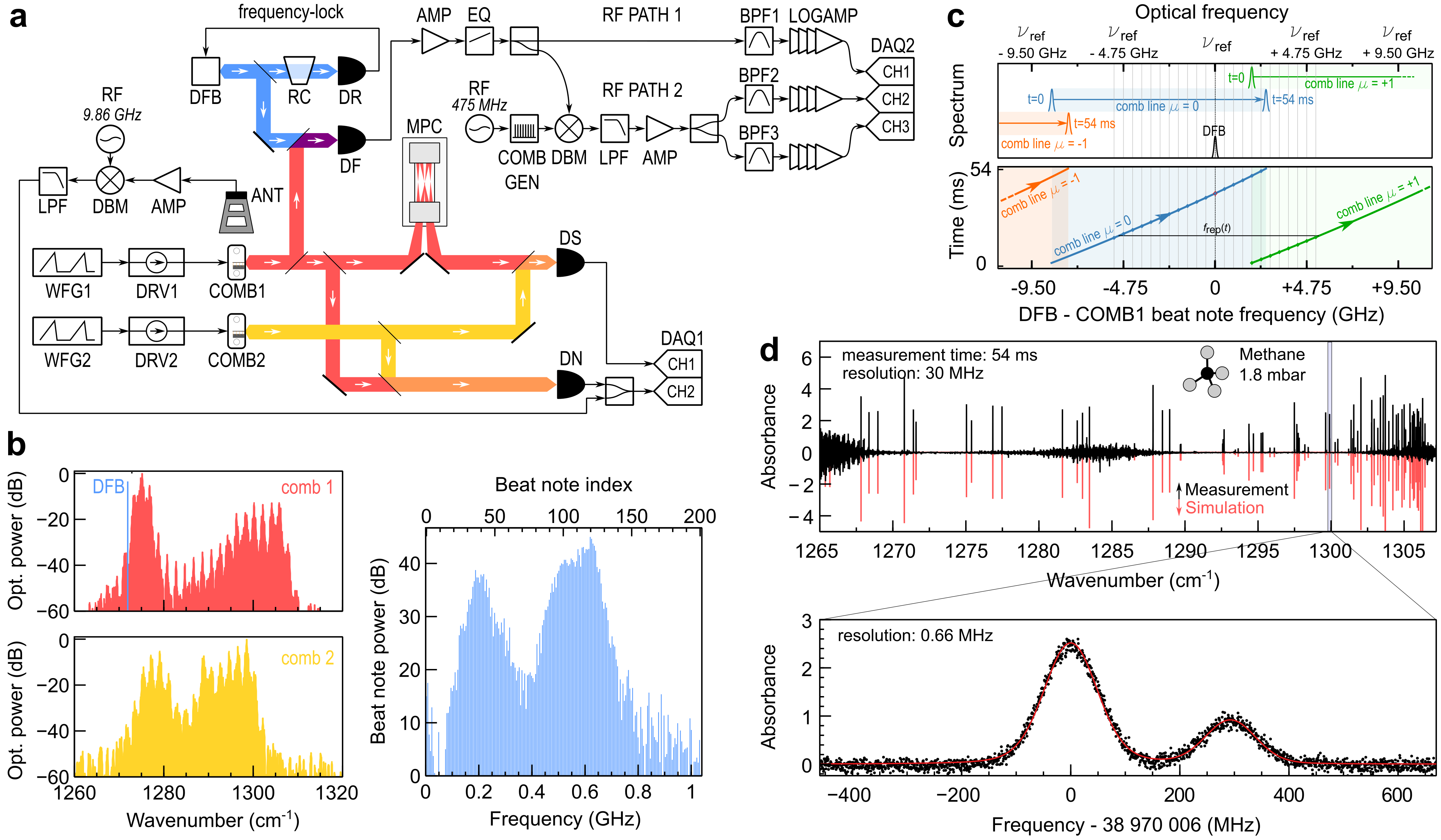
Figure 1: Experimental setup and schematic for accurate frequency scale. (a) Experimental setup featuring the distributed feedback (DFB) laser serving as frequency reference, the gapless dual comb spectrometer, and the setups to measure the repetition rate and the optical frequency during an acquisition. MPC: multi-pass cell, AMP: amplifier, BPF, LPF: band-pass (low-pass) filter, DBM: double-balanced mixer, LOGAMP: logarithmic amplifier, EQ: equalizer, COMB GEN: comb generator, WFG: waveform generator, DAQ: data acquisition unit, DS, DN, DR, DF: photodetector (see main text). (b) Optical spectra of COMB1, COMB2, the position of the reference DFB laser, and the multi-heterodyne beat spectrum. (c) Schematic of the referencing scheme of the optical frequencies of COMB1 while they are tuned across more than one free-spectral range ($f_{\mathrm{rep}}$), relying on the use of a synthetic comb. (d) Absorption spectrum of low pressure methane acquired in $54\,\mathrm{ms}$ by our spectrometer. The top panel is digitally filtered for visibility while the lower panel features two absorption lines at the original resolution of $660\,\mathrm{kHz}$.

Our dual-comb spectrometer is composed of two QCL frequency combs Gianella et al. (2020) (COMB1 and COMB2) is schematized in Fig. 1(a). COMB1 is the interrogating comb which probes the sample contained in a multi-pass cell, and COMB2 is the local oscillator. The repetition frequency of the combs, $f_{\mathrm{rep}}\approx 9.88\,\mathrm{GHz}$, is too large to sample Doppler-broadened gas-phase spectra of small molecules. Therefore, we tune the driving current to scan the comb lines across $f_{\mathrm{rep}}$ and interleave spectra to reduce the spectral point spacing by 4 orders of magnitude. The local oscillator comb is tuned synchronously to keep the multi-heterodyne spectrum within the detection bandwidth of the system [see Fig. 1(b)]. The interferograms measured on the photodetectors DS and DN are divided into slices of length $\tau=13.1\,\mathrm{\mu s}$, which are sufficiently long to resolve the beat notes (beat note spacing, $\Delta f_{\mathrm{rep}}\approx 4.5\,\mathrm{MHz}$). A lower limit for the spectral resolution, $\delta\nu=\dot{\nu}\cdot(\tau/3.77)$, can be estimated from the slice length, $\tau$, and the tuning rate, $\dot{\nu}$. The factor $3.77$ stems from the employed flattop apodization. For the tuning rates (scan duration) $\dot{\nu}=380\,\mathrm{GHz/s}$ $(27\,\mathrm{ms})$, $190\,\mathrm{GHz/s}$ $(54\,\mathrm{ms})$, $95\,\mathrm{GHz/s}$ $(107\,\mathrm{ms})$, and $47\,\mathrm{GHz/s}$ $(215\,\mathrm{ms})$ (see below) we find, respectively, $\delta\nu=1.3\,\mathrm{MHz},\,660\,\mathrm{kHz},\,330\,\mathrm{kHz},\,160\,\mathrm{kHz}$. For example, the spectrometer can acquire spectra spanning $40\,\mathrm{cm^{-1}}$ in $54\,\mathrm{ms}$ at a point spacing and resolution of $0.66\,\mathrm{MHz}$, allowing measurement of low-pressure methane [see Fig. 1(d)]. The noise-equivalent absorbance and noise-equivalent absorption coefficient depend on the signal-to-noise ratio (SNR) of the corresponding beat note [see Fig. 1(b)]. For strong beat notes, they are of the order of $3\times 10^{-4}\,\mathrm{Hz^{-1/2}}$ and $8\times 10^{-8}\,\mathrm{cm^{-1}Hz^{-1/2}}$, respectively, given the absorption path length of $36\,\mathrm{m}$ in the multi-pass cell.

The distributed feedback QCL (DFB) is locked to a molecular transition ($\mathrm{N_{2}O}$, fundamental $\nu_{1}$ band, P(14)) and acts as optical frequency reference with frequency $\nu_{\mathrm{ref}}$ Komagata et al. (2022). The beat frequency, $f_{b}$, between the reference laser and COMB1 is detected on a $1.2\,\mathrm{GHz}-$bandwidth detector (DF). The frequency, $\nu_{\mu}(t)$, of all lines, $\mu=0,\pm 1,\pm 2,...$, of the interrogating comb over the time of the scan is computed from the measured repetition rate, $f_{\mathrm{rep}}(t)$, and beat frequency, $f_{b}(t)$, at each instant of the sweep, and is given by

$$\nu_{\mu}(t)=\nu_{\mathrm{ref}}+f_{b}(t)+\mu\cdot f_{\mathrm{rep}}(t).$$ (1)

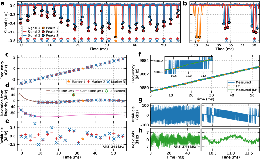
Figure 2: Assessment of $f_{b}$ and $f_{\mathrm{rep}}$ over a gapless measurement (sweep range $\geq f_{\mathrm{rep}}$). (a) Filtered marker signal as a function of time (solid lines) and peaks localized by the algorithm (filled circles). The mean position of two peaks gives the marker position shown by a star, plus or x. (b) Zoom over 3 pairs of peaks. (c) Frequency of the markers as a function of time. (d) Frequency of the markers minus the linear trend and polynomial fitting of the comb line frequency. The first 4 pairs of marker originate from the beat with another comb line ($\mu=1$ instead of $\mu=0$). (e) Residuals from the fit from (d). (f) Measured $f_{\mathrm{rep}}$ using two methods as a function of time and fit. The inset shows the a zoom over a smaller time interval. (g,h) Residuals of $f_{\mathrm{rep}}$ measured through the fast processor (g), which is limited by the integration time, or measured with high resolution (H.R.) (h). The right plot shows a zoom over a smaller interval. The fit using the processor data is accurate for the H.R. data within 2.4 kHz.

The measurement of $f_{b}(t)$ is based on the open-loop solution proposed in 2009 by Del’Haye et al. Del’Haye et al. (2009) with a few notable changes. Here, the reference laser is fixed while the comb is swept by approximately $f_{\mathrm{rep}}$. Therefore, a single pair of peaks is detected through RF path 1 [see Fig. 1(a)]. These are observed at the instants when the band-pass filter BPF1 transmits the beat to the rectifying logarithmic amplifier (LOGAMP). The recorded signal on channel 1 of DAQ2 is shown in Fig. 2(a,b) as Signal 1.

We implement a second RF path [RF path 2, see Fig. 1(a)], where we mix the beat with a $f_{\mathrm{RF}}=475\,\mathrm{MHz}$-spaced harmonic RF comb. The RF comb provides a synthetic grid of frequencies centered on the reference laser frequency, $\nu_{\mathrm{ref}}$, and having a spacing of $f_{\mathrm{RF}}$ [see Fig. 1(c)], whereby the time of passage of $\nu_{0}$ across each grid line is measured. Hence, the determination of $f_{b}(t)$ (or $\nu_{0}(t)$) is based on the measurement of the times at which $f_{b}$ equals multiples of $f_{\mathrm{RF}}$. These markers allow to map the frequency of $f_{b}(t)$ (or $\nu_{0}(t)$) versus time, as shown in Fig. 2(c). The marker on channel 1 allows identification of $\nu_{0}(t_{0})$ modulo $f_{\mathrm{rep}}$.

The $5\,\mathrm{GHz}$ RF bandwidth required to measure $f_{b}$ throughout the sweep, corresponding to $f_{\mathrm{rep}}/2$, poses a challenge, as the specified bandwidth of the photodetector is only $1.2\,\mathrm{GHz}$. We thus used logarithmic amplifiers to increase the marker detection dynamic range and gain equalizers (EQ) to reduce signal strength imbalances. Moreover, in order to further balance the signal strength and optimize the RF mixers, the signals were split below and above $3.8\,\mathrm{GHz}$ [not shown in Fig. 1(c)]. Further information can be found in Methods and Supplementary Note 1.

We plot the markers after removal of the linear trend in Fig. 2(d). The first 4 sets of markers originate from the beating with a higher comb line $\mu=1$ [see Fig. 1(c)], which was unavoidable to accommodate a sweep about 10 % larger than $f_{\mathrm{rep}}$. We fit the markers with a 10th order polynomial using a two comb line model separated by $f_{\mathrm{rep}}(t)$. The algorithm is robust against spurious peaks, which produce markers that can be discarded if they don’t fit within a certain tolerance region. The residuals of the fit are shown in Fig. 2(e). The standard deviation of the fit residuals is found to be $241\,\mathrm{kHz}$.

The repetition rate, detected by the horn antenna, is down-mixed to $\sim 20\,\mathrm{MHz}$, digitized on DAQ1, channel 2, and processed together with the interferogram [see Fig. 1(a)]. The resolution is limited to $76\,\mathrm{kHz}$ due to the finite length ($\tau=13.1\,\mathrm{\mu s}$) of the slices [see Fig. 2(f)]. We fit these data using a 10th order polynomial. The residuals are limited by the resolution as shown in Fig. 2(g,h). On a control measurement, we recorded the raw digitized data from DAQ1, channel 2, and computed $f_{\mathrm{rep}}(t)$ with higher resolution. The residuals between the fit from the low resolution data and the high resolution data are shown in Fig. 2(h), showing correspondence within $2.4\,\mathrm{kHz}$. The high-resolution data feature oscillations of $f_{\mathrm{rep}}$ due to back-reflection from the photodetectors.

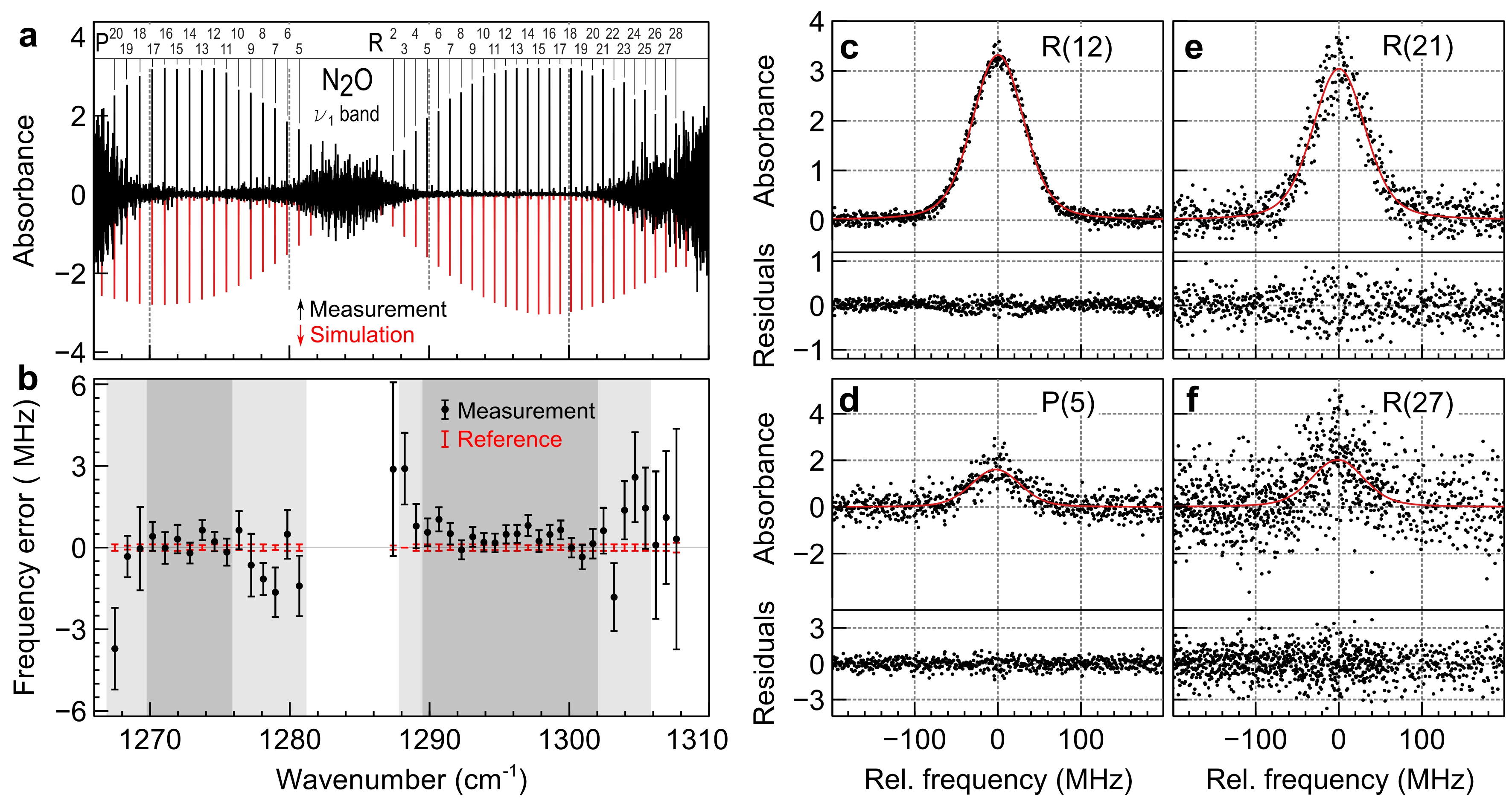
Figure 3: Spectra and retrieved line centers in a $54\,\mathrm{ms}$ acquisition (a) Single shot spectra of the $\nu_{1}$ fundamental band of nitrous oxide with $660\,\mathrm{kHz}$ spectral point spacing, acquired in 54-ms and comparison with simulation. (b) Retrieved line centers compared with literature reference with 1-$\sigma$ error bars. (c-f) Zoom of (e) on 4 different lines illustrating stronger/weaker absorbance and high/low SNR, and residuals of the Voigt fit shown in red.

Figure 3(a) shows a spectrum of the fundamental $\nu_{1}$ band of nitrous oxide acquired in a single sweep of $54\,\mathrm{ms}$. The bimodal comb amplitude distribution gives rise to a variable SNR across the spectrum, as can be seen in Figs. 3(c-f). We used a Voigt fit to retrieve the line centers of the molecular transitions.

We benchmark the frequency accuracy of our spectrometer by comparing the computed line center frequencies to those obtained by two other groups with 100-kHz level accuracy AlSaif et al. (2018); Hjältén et al. (2021). Based on multiple sets of measurements over the course of a few weeks, we estimate that we retrieve, in a single-shot acquisition, 40 line centers (spanning $30.4\,\mathrm{cm^{-1}}$) with a 1-$\sigma$ accuracy better than $2\,\mathrm{MHz}$, among which 23 lines (spanning $17.1\,\mathrm{cm^{-1}}$) are retrieved with an accuracy better than $0.6\,\mathrm{MHz}$, as can be seen in Fig. 3(b).

This estimation includes the uncertainties of the reference laser frequency $\nu_{\mathrm{ref}}$ ($180\,\mathrm{kHz}$ after correction of a systematic bias of $(180\pm 100)\,\mathrm{kHz}$), $f_{\mathrm{rep}}$ ($2.6\,\mathrm{kHz}$ after the correction of a systematic bias of $(2.9\pm 0.7)\,\mathrm{kHz}$), the fit of the markers as in Fig. 2(e) ($240\,\mathrm{kHz}$), and the standard deviation of the retrieved line center frequencies over 12 consecutive 54-ms measurements (below $300\,\mathrm{kHz}$ for the lines with the best SNR, see Fig. 4). The retrieved line centers and the uncertainties are consistent with the literature values.

The frequency accuracy of the spectrometer allows us to retrieve the line centers of $\mathrm{CH_{4}}$ with a higher accuracy than the current literature Gordon et al. (2022). Our results are given in Table 1. For this measurement, we averaged the retrieved line centers over 15 measurements.

Transition	Line center
(J’,C’,$\alpha$’) - (J”,C”,$\alpha$”)	(cm-1)
[ head to column names, separator=semicolon, late after line=
, late after last line=

Table 1: Measured line list of the methane $\nu_{4}$ band. The upper (lower) levels are labeled with a single (double) prime and are denoted according to the Hitran Gordon et al. (2022) notation.

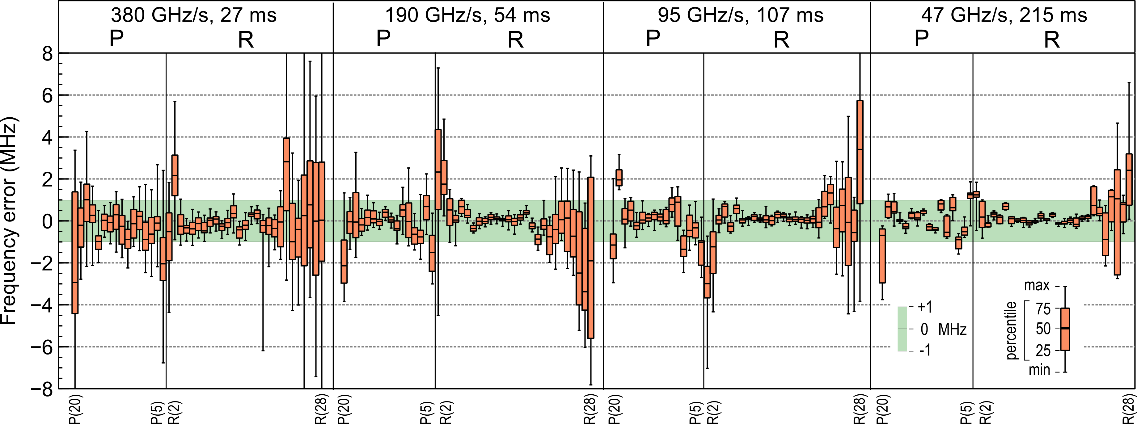
Figure 4: Frequency precision for varying scanning speed. Frequency error and statistical spread of the retrieved line centers at 4 different scan speeds, decreasing from left to right by factors of 2. The precision increases with the scan time.

The scanning speed of the spectrometer can be varied to measure spectra in between $27\,\mathrm{ms}$ to $216\,\mathrm{ms}$. We estimate an accumulated chirp Riemensberger et al. (2020) rate of $44\,\mathrm{THz/s}$ to $5.6\,\mathrm{THz/s}$, considering 120 lines which sweep in parallel.

The sweep becomes discontinuous at faster rates. Slower tuning is possible, but requires a larger buffer in the acquisition unit.

Figure 4 displays the statistics in the form of box plots of the retrieved $\mathrm{N_{2}O}$ line centers with respect to literature reference for varying scanning speeds. Scan speeds up to $380\,\mathrm{GHz/s}$ do not induce noticeable offsets in the retrieved line centers, within the uncertainties. This shows that delays due to the RF scheme are negligible. The measurement at 380 GHz/s was performed at a later date. Potential delays at faster scanning speeds could be assessed and corrected from a reference measurement.

We have demonstrated a fast and accurate mid-infrared dual-comb spectrometer. The combs were emitted by quantum cascade lasers, which can be tuned over their free spectral range ($f_{\mathrm{rep}}$) in tens of milliseconds to provide high-resolution spectra of broad molecular bands. We calibrated the frequency axis by measuring the beat between the interrogating comb and a reference laser and by acquiring the comb’s repetition rate. Moreover, we have enhanced the marker method Del’Haye et al. (2009) using a synthetic comb, to process the fast chirp of the beat between the comb and the reference laser. This method is compatible with other integrated comb technologies featuring multi-GHz repetition frequencies such as micro-resonator combs Kippenberg et al. (2018), and could also be applied to comb-calibrated spectroscopy Del’Haye et al. (2009).

Thus, our agile spectrometer provides unique performances in terms of acquisition speed and frequency accuracy compared to other broadband spectrometers with small ($<10\,\mathrm{MHz}$) spectral point spacing Del’Haye et al. (2009); Nishiyama et al. (2013); AlSaif et al. (2018); Gotti et al. (2020); Hjältén et al. (2021). Our spectrometer is a promising candidate towards an on-chip gas sensor that is highly sensitive and selective to many relevant molecules, allowing real-time monitoring of complex gas mixtures at Hz-level refresh rates.

Finally, we believe that the spectrometer sensitivity, bandwidth, and power-efficiency will improve thanks to ongoing development in quantum cascade laser frequency combs, such as mutual stabilization Komagata et al. (2021); Hillbrand et al. (2022), dispersion management Villares et al. (2016), and full spectrometer integration Schwarz et al. (2014).

III Methods

III.1 Experimental setup

The two laser sources were InGaAs/AlInAs on InP-based dual-stack QCLs Jouy et al. (2017); Gianella et al. (2020). They were $4.5\,\mathrm{mm}$ long ($f_{\mathrm{rep}}\approx 9.88\,\mathrm{GHz}$, $\Delta f_{\mathrm{rep}}\approx 4.5\,\mathrm{MHz}$) and had both end facets uncoated. The combs emitted several hundred mW of optical power over $\sim 50\,\mathrm{cm^{-1}}$ in the $1300\,\mathrm{cm^{-1}}$ range [see Fig. 1(b)]. They were operated at constant temperature of $1.9^{\circ}\mathrm{C}$ and $2.2^{\circ}\mathrm{C}$, respectively. The combs were electrically driven by a pair of QubeCL drivers (ppqSense). The bias currents for the two combs were $1532\,\mathrm{mA}$ and $1226\,\mathrm{mA}$, respectively. The currents were modulated by asymmetric triangular waveforms (WFG1 and WFG2 are the two outputs of an ArbStudio 1102, LeCroy waveform generator) with the currents initially decreasing at constant rate during a time $T=30\,\mathrm{ms}$, $60\,\mathrm{ms}$, $120\,\mathrm{ms}$, or $240\,\mathrm{ms}$ and returning to the initial value over a shorter time $0.25\cdot T$. The peak-to-peak current modulation amplitude was approximately $90\,\mathrm{mA}$ for both lasers. This required a modification of the QubeCL drivers which, by default, do not allow such large current modulations. The beam splitters were custom-made to obtain the appropriate power ratios at each photodetector. They were designed for reflecting 1%, 10% or 50% at an angle of incidence of 45° for s-polarized light from 1220-1370$\,\mathrm{cm}^{-1}$. They were produced by ion beam sputtering (IBS) on 5 mm thick wedged (0.5 deg) $\mathrm{CaF_{2}}$ substrates with an anti-reflection coating on the back side to minimize undesired interference effects.

Two $1\,\mathrm{GHz}-$bandwidth MIR photodetectors were employed to measure the sample (DS) and to normalize laser intensity and phase noise (DN). The detector outputs were sampled at $2.5\,\mathrm{GSa/s}$ with 12 bit resolution by the data acquisition unit DAQ1 (ADQ32, Teledyne), generating $10\,\mathrm{Gbyte/s}$ of raw data for the duration of the sweep. The data acquisition was triggered at $t=0.07\cdot T$ after the start of the (decreasing) current ramp and continued for a duration of $27\,\mathrm{ms}$, $54\,\mathrm{ms}$, $107\,\mathrm{ms}$, or $215\,\mathrm{ms}$, which corresponds to $2^{26}$, $2^{27}$, $2^{28}$, or $2^{29}$ samples at $2.5\,\mathrm{GSa/s}$. The clocks of DAQ1 (Fig. 1(a)) and of the synthesizer generating the $475\,\mathrm{MHz}$ fundamental for the synthetic comb generator were referenced to a GPS-disciplined clock (GPSDO, Leo Bodnar).

A custom software (C++ and CUDA) was used to process the two interferograms. The program is capable of fully processing (from raw data to absorbance values) 25 $27\,\mathrm{ms}$-long sweeps per second, corresponding to a raw data throughput of $6.75\,\mathrm{Gbyte/s}$, or 67.5% of the maximum raw data input rate. The interferograms were first divided into slices of length $2^{15}=32,768$ samples, corresponding to $13.1\,\mathrm{\mu s}$. The beat note amplitudes were computed for each slice by fast Fourier transform, from which the sample’s absorbance was determined.

A distributed feedback QCL (DFB, Alpes Lasers) emitting a continuous wave (cw) beam was locked to a molecular transition ($\mathrm{N_{2}O}$, fundamental $\nu_{1}$ band, P(14)) by means of a wavelength modulation scheme and acted as optical frequency reference with frequency $\nu_{\mathrm{ref}}$.

III.2 Measurement of the markers and retrieval of the frequency axis

The heterodyne beat between the DFB reference laser and COMB1 is detected on the fast photodetector (UHSM-10.6 PV-4TE-10.6-0.05-butt, Vigo System). Through RF path 1, two pulses are transmitted in rapid succession when $f_{b}(t)$ passes near zero and are amplified by a logarithmic amplifier (ZX47-60LN-S+, Minicircuits). The timings of the two peaks, $t_{0}^{\pm}$, fulfill $f_{b}(t_{0}^{\pm})=\pm f_{\mathrm{bp,1}}$, where $f_{\mathrm{bp,1}}=25\,\mathrm{MHz}$ is the center frequency of BPF1. We assume linear chirping of the beat between $t_{0}^{-}$ and $t_{0}^{+}$, so that $f_{b}(t_{0})=0$, where $t_{0}$ is the mean of $t_{0}^{+}$ and $t_{0}^{-}$. With Eq. 1 we find $\nu_{0}(t_{0})=\nu_{\mathrm{ref}}$.

As for RF path 2, $f_{b}(t)$ is mixed with an RF comb with spacing $f_{\mathrm{RF}}$. Therefore, each time the DFB-comb beat, $f_{b}(t)$, nears a multiple of $f_{\mathrm{RF}}$, two double pulses are recorded on channels 2 and 3 of DAQ2 (Signal 2 and Signal 3 in Fig. 2(a,b)). The timings, $t_{n}^{\pm}$ of the two pulses of the $n$th ($n=\pm 1,\pm 2,...$) double pulse fulfill $f_{b}(t_{n}^{\pm})=n\cdot f_{\mathrm{RF}}\pm f_{\mathrm{bp,i}}$, where $f_{\mathrm{bp,2}}=21\,\mathrm{MHz},f_{\mathrm{bp,3}}=45\,\mathrm{MHz}$ are the center frequencies of BPF2 and BPF3, respectively. For the mean times, $t_{n}=(t_{n}^{-}+t_{n}^{+})/2$, we find, as before, $f_{b}(t_{n})=n\cdot f_{\mathrm{RF}}$ and with Eq. 1, $\nu_{0}(t_{n})=\nu_{\mathrm{ref}}+n\cdot f_{\mathrm{RF}}$. More details concerning the processing of the markers can be found in Supplementary Figure 1 and Supplementary Note 1.

As post-processing, we first smooth the marker signals with a low-pass filter. Then we detect the peaks which match specific criteria in terms of prominence, width, and proximity to other lines using a peak-finding algorithm (find_peaks, scipy). If two peaks have the appropriate time delay, we establish that $f_{b}$ was at a multiple integer $n$ of $f_{\mathrm{RF}}$ at the mean time of the two peaks. The integer $n$ is guessed from linear interpolation using marker 1 and an estimated chirp. The discontinuity from the change of comb line can be easily recognized and the markers originating from comb line $\mu=1$ can be used to determine the frequency of comb line $\mu=0$ by knowledge of $f_{\mathrm{rep}}(t)$.

We fit the markers with polynomials of increasing orders up to 10, keeping the coefficients of the previous order as initial guess and providing the initial guess for the new coefficient from the residuals of the previous fit. A larger weight is given to marker 2 as BPF2 is narrower than the other band-pass filters. After the fits with the $4^{\mathrm{th}}$ and $8^{\mathrm{th}}$ order polynomial, markers outside a tolerance of $50\,\mathrm{MHz}$ and $10\,\mathrm{MHz}$ are discarded, respectively. This allows the removal of most spurious peaks, which do not align in the plot Fig. 2(d).

III.3 Measurement of the repetition rate

In QCL frequency combs, the beating of all co-existing modes in the laser produces a measurable voltage modulation on the laser electrodes with frequency equal to $f_{\mathrm{rep}}$ Piccardo et al. (2018). The laser module features a $50\,\mathrm{\Omega}$ transmission line on a printed circuit board that connects an SMA connector at the back of the housing to a point very close (within $1\,\mathrm{mm}$) to the back facet of the laser. From there, a short bond wire establishes an electrical connection to the laser’s top electrode. This pathway can be used for RF injection or to measure $f_{\mathrm{rep}}$. However, connecting cables and other circuitry to the SMA port tends to increase laser phase noise. It is observable as a broadening of the beat notes. Therefore, a horn antenna (ANT, PowerLOG 40040, Aaronia) was pointed at the open SMA connector. The detected $f_{\mathrm{rep}}$ was then amplified and down-mixed to $\sim 20\,\mathrm{MHz}$ to enable its measurement on one channel of DAQ1.

III.4 Gas sample preparation and measurement

We dynamically diluted $\mathrm{N_{2}O}$ gas with nitrogen to a concentration of about of $450\,\mathrm{ppmv}$ and flowed the diluted mixture through the multi-pass cell (MPC). We then closed off the cell and pumped down to $1.5\,\mathrm{mbar}$, which provided sufficiently strong absorption lines and sufficiently low pressure to be reasonably close to the Doppler-broadened limit and, more importantly, to minimize the pressure-induced shift on the measured transitions. Multiple sweeps were taken but not averaged together. The time delay between sweeps was several seconds, to ensure proper synchronization of the two data sets acquired by the two DAQs, which were read out by independent software. By integrating both DAQs in the same processing routine, the acquisition rate (sweeps per unit time) could be increased significantly (about 12 $54\,\mathrm{ms}$-long sweeps per second).

References

References

- Hugi et al. (2012) A. Hugi, G. Villares, S. Blaser, H. C. Liu, and J. Faist, Nature 492, 229 (2012).
- Klocke et al. (2018) J. L. Klocke, M. Mangold, P. Allmendinger, A. Hugi, M. Geiser, P. Jouy, J. Faist, and T. Kottke, Anal. Chem. 90, 10494 (2018).
- Schwarz et al. (2014) B. Schwarz, P. Reininger, D. Ristanić, H. Detz, A. M. Andrews, W. Schrenk, and G. Strasser, Nat. Commun. 5, 4085 (2014).
- Kippenberg et al. (2018) T. J. Kippenberg, A. L. Gaeta, M. Lipson, and M. L. Gorodetsky, Science 361, eaan8083 (2018).
- Bagheri et al. (2018) M. Bagheri, C. Frez, L. A. Sterczewski, I. Gruidin, M. Fradet, I. Vurgaftman, C. L. Canedy, W. W. Bewley, C. D. Merritt, C. S. Kim, M. Kim, and J. R. Meyer, Sci. Rep. 8, 3322 (2018).
- Kuse et al. (2021) N. Kuse, G. Navickaite, M. Geiselmann, T. Yasui, and K. Minoshima, Opt. Lett. 46, 3400 (2021).
- Gianella et al. (2022) M. Gianella, S. Vogel, V. J. Wittwer, T. Südmeyer, J. Faist, and L. Emmenegger, Opt. Lett. 47, 625 (2022).
- Lepère et al. (2022) M. Lepère, O. Browet, J. Clément, B. Vispoel, P. Allmendinger, J. Hayden, F. Eigenmann, A. Hugi, and M. Mangold, J. Quant. Spectrosc. Radiat. Transf. , 108239 (2022).
- Gianella et al. (2020) M. Gianella, A. Nataraj, B. Tuzson, P. Jouy, F. Kapsalidis, M. Beck, M. Mangold, A. Hugi, J. Faist, and L. Emmenegger, Opt. Express 28, 6197 (2020).
- Riemensberger et al. (2020) J. Riemensberger, A. Lukashchuk, M. Karpov, W. Weng, E. Lucas, J. Liu, and T. J. Kippenberg, Nature 581, 164 (2020).
- Del’Haye et al. (2009) P. Del’Haye, O. Arcizet, M. L. Gorodetsky, R. Holzwarth, and T. J. Kippenberg, Nat. Photonics 3, 529 (2009).
- Coddington et al. (2016) I. Coddington, N. Newbury, and W. Swann, Optica 3, 414 (2016).
- Giorgetta et al. (2021) F. R. Giorgetta, J. Peischl, D. I. Herman, G. Ycas, I. Coddington, N. R. Newbury, and K. C. Cossel, Laser Photonics Rev. 15, 2000583 (2021).
- Vicentini et al. (2021) E. Vicentini, Z. Wang, K. Van Gasse, T. W. Hänsch, and N. Picqué, Nat. Photonics 15, 890 (2021).
- Parriaux et al. (2022) A. Parriaux, K. Hammani, C. Thomazo, O. Musset, and G. Millot, Phys. Rev. Research 4, 023098 (2022).
- Villares et al. (2014) G. Villares, A. Hugi, S. Blaser, and J. Faist, Nat. Commun. 5, 5192 (2014).
- Muraviev et al. (2020) A. V. Muraviev, D. Konnov, and K. L. Vodopyanov, Sci. Rep. 10, 18700 (2020).
- Luo (2020) P.-L. Luo, Opt. Lett. 45, 6791 (2020).
- Hjältén et al. (2021) A. Hjältén, M. Germann, K. Krzempek, A. Hudzikowski, A. Głuszek, D. Tomaszewska, G. Soboń, and A. Foltynowicz, J. Quant. Spectrosc. Radiat. Transf. 271, 107734 (2021).
- Benkler et al. (2013) E. Benkler, F. Rohde, and H. R. Telle, Opt. Express 21, 5793 (2013).
- Germann et al. (2022) M. Germann, A. Hjältén, V. Boudon, C. Richard, K. Krzempek, A. Hudzikowski, A. Głuszek, G. Soboń, and A. Foltynowicz, arXiv:2204.06356 (2022).
- Komagata et al. (2022) K. N. Komagata, M. Gianella, P. Jouy, F. Kapsalidis, M. Shahmohammadi, M. Beck, R. Matthey, V. J. Wittwer, A. Hugi, J. Faist, L. Emmenegger, T. Südmeyer, and S. Schilt, Opt. Express 30, 12891 (2022).
- AlSaif et al. (2018) B. AlSaif, M. Lamperti, D. Gatti, P. Laporta, M. Fermann, A. Farooq, O. Lyulin, A. Campargue, and M. Marangoni, J. Quant. Spectrosc. Radiat. Transf. 211, 172 (2018).
- Gordon et al. (2022) I. Gordon, L. Rothman, R. Hargreaves, R. Hashemi, E. Karlovets, F. Skinner, E. Conway, C. Hill, R. Kochanov, Y. Tan, P. Wcisło, A. Finenko, K. Nelson, P. Bernath, M. Birk, V. Boudon, A. Campargue, K. Chance, A. Coustenis, B. Drouin, J. Flaud, R. Gamache, J. Hodges, D. Jacquemart, E. Mlawer, A. Nikitin, V. Perevalov, M. Rotger, J. Tennyson, G. Toon, H. Tran, V. Tyuterev, E. Adkins, A. Baker, A. Barbe, E. Canè, A. Császár, A. Dudaryonok, O. Egorov, A. Fleisher, H. Fleurbaey, A. Foltynowicz, T. Furtenbacher, J. Harrison, J. Hartmann, V. Horneman, X. Huang, T. Karman, J. Karns, S. Kassi, I. Kleiner, V. Kofman, F. Kwabia–Tchana, N. Lavrentieva, T. Lee, D. Long, A. Lukashevskaya, O. Lyulin, V. Makhnev, W. Matt, S. Massie, M. Melosso, S. Mikhailenko, D. Mondelain, H. Müller, O. Naumenko, A. Perrin, O. Polyansky, E. Raddaoui, P. Raston, Z. Reed, M. Rey, C. Richard, R. Tóbiás, I. Sadiek, D. Schwenke, E. Starikova, K. Sung, F. Tamassia, S. Tashkun, J. Vander Auwera, I. Vasilenko, A. Vigasin, G. Villanueva, B. Vispoel, G. Wagner, A. Yachmenev, and S. Yurchenko, J. Quant. Spectrosc. Radiat. Transf. 277, 107949 (2022).
- Nishiyama et al. (2013) A. Nishiyama, D. Ishikawa, and M. Misono, J. Opt. Soc. Am. B 30, 2107 (2013).
- Gotti et al. (2020) R. Gotti, T. Puppe, Y. Mayzlin, J. Robinson-Tait, S. Wójtewicz, D. Gatti, B. Alsaif, M. Lamperti, P. Laporta, F. Rohde, R. Wilk, P. Leisching, W. G. Kaenders, and M. Marangoni, Sci. Rep. 10, 2523 (2020).
- Komagata et al. (2021) K. Komagata, A. Shehzad, G. Terrasanta, P. Brochard, R. Matthey, M. Gianella, P. Jouy, F. Kapsalidis, M. Shahmohammadi, M. Beck, V. J. Wittwer, J. Faist, L. Emmenegger, T. Südmeyer, A. Hugi, and S. Schilt, Opt. Express 29, 19126 (2021).
- Hillbrand et al. (2022) J. Hillbrand, M. Bertrand, V. Wittwer, N. Opacak, F. Kapsalidis, M. Gianella, L. Emmenegger, B. Schwarz, T. Südmeyer, M. Beck, and J. Faist, arXiv:2202.09620 (2022).
- Villares et al. (2016) G. Villares, S. Riedi, J. Wolf, D. Kazakov, M. J. Süess, P. Jouy, M. Beck, and J. Faist, Optica 3, 252 (2016).
- Jouy et al. (2017) P. Jouy, J. M. Wolf, Y. Bidaux, P. Allmendinger, M. Mangold, M. Beck, and J. Faist, Appl. Phys. Lett. 111, 141102 (2017).
- Piccardo et al. (2018) M. Piccardo, D. Kazakov, N. A. Rubin, P. Chevalier, Y. Wang, F. Xie, K. Lascola, A. Belyanin, and F. Capasso, Optica 5, 475 (2018).