Improved background model for the Large Area X-ray Proportional Counter (LAXPC) instrument on-board AstroSat

Abstract

We present an improved background model for the Large Area X-ray Proportional Counter (LAXPC) detectors on-board AstroSat. Because of the large collecting area and high pressure, the LAXPC instrument has a large background count rate, which varies during the orbit. Apart from the variation with latitude and longitude during the orbit there is a prominent quasi-diurnal variation which has not been modelled earlier. Using over 5 years of background observations, we determined the period of the quasi-diurnal variation to be 84495 s and using this period, it is possible to account for the variation and also identify time intervals where the fit is not good. These lead to a significant improvement in the background model. The quasi-diurnal variation can be ascribed to the changes in charged particle flux in the near Earth orbit.

1 Introduction

The Large Area X-ray Proportional Counter (LAXPC) instrument aboard the Indian Astronomy mission AstroSat consists of 3 co-aligned large area proportional counter units for X-ray timing and spectral studies over an energy range of 3–80 keV (Agrawal, 2006; Yadav et al., 2016; Agrawal et al., 2017). The detailed calibration of LAXPC instrument, including the background model was described by Antia et al. (2017, 2021). AstroSat was launched on 28 September 2015 and has completed six years in orbit. Currently, only one LAXPC detector, i.e., LAXPC20 is working nominally. Because of large size of the detector and a gas pressure of two atmospheres, the background rate is rather high, being about 200 c s^-1 in LAXPC20. There is also a strong variation in the background rate during each orbit with the maximum count rate being achieved near the South Atlantic Anomaly (SAA) passage. A large part of the orbital variation can be modelled by fitting the count rate as a function of latitude and longitude of the satellite (Antia et al., 2017, 2021). Apart from this, there is a quasi-diurnal variation with an amplitude of about 20 c s^-1 (Antia et al., 2021) which is not accounted for by the existing background models. This limits the effectiveness of background subtraction and hence the sensitivity of the instrument for faint sources as well as spectral studies at high energies for relatively bright sources. There is also a long term variation over the period of 6 years in the background count rate as well as the amplitude of quasi-diurnal trend.

An alternate background model has been implemented by Misra et al. (2021) which is applicable only for faint sources and is restricted to the top layer of the detector. This model is based on the assumption that for faint sources the counts at high energies are only contributed by the background, which can be scaled to get the background at low energies. This model is sensitive to gain shift in the detectors and hence is only applicable to LAXPC20 which has relatively stable gain. This happens to be the only detector which has been working nominally after April 2018. This model can account for the quasi-diurnal trend to some extent, but its applicability is limited to faint sources and the top layer of the detector. Further, the calibration of this model has not been updated and hence it doesn’t work so well on recent observations and in fact the diurnal variation is not removed (Figure 15 of Antia et al., 2021).

The main difficulty in accounting for the quasi-diurnal trend was that its exact period was not known. During the initial years the amplitude of this signal was also smaller. With increasing amplitude of the trend it became more important to understand this trend. Using more than 5 years of background observations and satellite orbital parameters, we have now identified the period of quasi-diurnal variation to be 84495 s, which allows us to remove the trend effectively and improve the background model.

The rest of the paper is organized as follows: Section 2 gives a summary of various periodicities in AstroSat orbit so that the observed periodicity in the background count rate can be identified with some of these. Section 3 describes the determination of periodicity in background count rate using over five years of background observation. Section 4 describes the application of this to background model and the resulting improvement. Section 5 gives the summary of the results.

2 The AstroSat orbit

AstroSat has been placed in a nearly circular orbit with eccentricity of $\sim 0.001$, altitude of about 640 km and a inclination of about $6^{\circ}$ to the equator. The altitude has been decreasing slowly with time, resulting in a slow decrease in the orbital period. During April 2021, the sidereal orbital period was 5844.38 s, while the period as measured by latitude variation was 5836.57 s, that from longitude was 6269.66 s and the altitude had a period of 5851.71 s. The frequency difference between the latitude and longitude gives a period of 84494 s. This differs from the sidereal rotation period of the Earth, 86164 s because of precession of the orbit.

Figure 1: The maximum and minimum altitude during each orbit and the maximum latitude during each orbit, is shown in the left panel as a function of days since the launch of AstroSat. The arrows in the top panel mark the times of AstroSat orbit maneuvers. The right panel shows the same quantities over a limited time to show the variations on scale of days.

Since the eccentricity of the orbit is very small the rate of precession of the nodes or the plane of the orbit can be estimated by considering the perturbation due to gravitational quadrupole moment, $J_{2}$ ($=0.00108$ for the Earth) to get the precession rate

$$\frac{3\pi R^{2}}{Ta^{2}}J_{2}\approx 1.44\times 10^{-6}\;\mbox{rad}\;\mbox{s}^{-1},$$ (1)

where, $R$ is the radius of the Earth, $a$ is the semi-major axis of the satellite orbit and $T$ is the orbital period of the satellite. This gives the precession period of about $4.36\times 10^{6}$ s. For nearly circular orbit this is also the period of precession of the orbital plane. Since the maximum latitude during the orbit is changing with time the orbital plane should be precessing.

To determine the actual period of precession of AstroSat orbit we examined the orbital data for over five years and determined the minimum and maximum of altitude and latitude during each orbit and the results are shown in Figure 1. The minimum in latitude is not shown as it is almost same in magnitude to the maximum. The right panel of the figure shows the blowup of the same, which clearly shows variation on quasi-diurnal period as well as variation on time scale of order of 50 days. For the maximum latitude these periods averaged over the last five years are 84496 s and 4363843 s. The latter should be the precession period. If the corresponding frequency is added to the Earth’s rotation frequency we get a period of 84496 s, which is close to the frequency difference between the latitude and longitude periods. This is also close to the period of quasi-diurnal variation found in the LAXPC background. The three arrows in the figure mark the times when some orbital maneuvers were carried out. These maneuvers can change the orbital period, but it was found that the change in the period of quasi-diurnal variation due to the last two maneuvers is less than 1 s and hence is not considered. We have not considered the period before April 4, 2016, when the first maneuver was performed as that would have changed the period significantly and we do not have enough data before that to determine the period accurately. There was also only one long background observation before this time. It is difficult to model the background during this initial period as there were some adjustments made to various parameters in the detector.

While analyzing the orbital data it was discovered that during four periods of about one day each, there is some anomaly in the orbital data. Since the LAXPC analysis software relies on the satellite position to determine the time of Earth occultation and SAA passage these data may not be processed correctly. The affected observations are listed in Table 1, which also gives the time interval that is affected in MJD. The data from this period should be rejected during analysis. The version v3.4 onward of LaxpcSoft (backshiftv3.f) would issue a warning if these data are processed.

Table 1: LAXPC observations affected by anomaly in orbital data

Observation ID	Source	Affected Period (MJD)
20180529_G08_025T01_9000002130	Cyg X-3	58268.25 – 58269.25
20200123_A07_138T09_9000003458	J164754.90+443345	58872.00 – 58873.30
20200910_A09_079T01_9000003864	CAL 83	59103.90 – 59105.00
20210120_A10_123T08_9000004126	BCD T8	59234.95 – 59235.90
20210121_A10_093T01_9000004128	2MASS J05215658+4359220	59234.95 – 59235.90

With the precession period obtained above, all the periodicities in AstroSat orbit can be explained. If $f_{A}=1/5844.38$ Hz is the sidereal frequency of AstroSat orbit, $f_{E}=1/86164$ Hz is the Earth’s rotation frequency and $f_{P}=1/4363843$ Hz is the precession frequency of AstroSat orbit, the frequencies, $f_{\mathrm{lat}},f_{\mathrm{lon}},f_{\mathrm{alt}}$ of the orbital period in longitude, latitude and altitude, respectively, can be determined as follows:

$$f_{\mathrm{lon}} = f_{A}-f_{E}={1\over 6269.64}\;\mathrm{Hz},$$ (2)

$$f_{\mathrm{lat}} = f_{A}+f_{P}={1\over 5836.56}\;\mathrm{Hz},$$ (3)

$$f_{\mathrm{alt}} = f_{A}-f_{P}={1\over 5852.22}\;\mathrm{Hz},$$ (4)

These values are all close to the observed periods mentioned earlier. Further,

$$f_{\mathrm{lat}}-f_{\mathrm{lon}}=f_{P}+f_{E}={1\over 84496}\;\mathrm{Hz}.$$ (5)

This is close to the actual frequency difference as noted earlier. As shown in the next section this is also close to the period of quasi-diurnal variation in the LAXPC background.

3 The period of quasi-diurnal variation in the background

To determine the period of quasi-diurnal variation in the background we use all background observations after April 4, 2016 covering a stare time of approximately a day or more. The light curves of all these observations with a time-bin of 10 s were combined into one time series. Only the Good Time Intervals (GTI) were considered, which exclude the passage through the South Atlantic Anomaly (SAA) and when the satellite is pointing to the Earth as the target location is occulted by the Earth. The dominant variation in the time-series is due to the orbital period of longitude, which gives the maximum count rate when the satellite is close to the SAA passage. Apart from this the quasi-diurnal oscillations are also seen (Antia et al., 2021). To fit both these periodic variations we fit the combined time series, $c(t)$, to the function

$$c(t)=a_{0}+\sum_{j=1}^{N}\left(a_{j}\cos(2\pi jf_{1}t)+b_{j}\sin(2\pi jf_{1}t)+d_{j}\cos(2\pi jf_{2}t)+e_{j}\sin(2\pi jf_{2}t)\right),$$ (6)

where, $f_{1},f_{2}$ are respectively, the frequencies of the orbital and quasi-diurnal variations and $N$ is the number of harmonics used in the fits. The parameters $a_{j},b_{j},d_{j},e_{j}$ and frequencies $f_{1},f_{2}$ are fitted to minimize the resulting $\chi^{2}$ deviation. $N=5$ was used in the fits as that was found to be sufficient.

Figure 2: The least square fit to background light curves, showing the reduced $\chi^{2}$ as a function of the quasi-diurnal period in the bottom panel and the resulting profile as a function of phase in the top panel.

Figure 3: The light curves for a few selected background observations in LAXPC20 with a time-bin of 32 s are shown as a function of $\mathrm{mod}(t,84495\;{\rm s})$. Since the background observations cover a period longer than 84495 s, there is some time period where multiple values are available.

The resulting least squares fit gives the two periods as 6270.40 s and 84495 s. The statistical errors in the fits were small and hence are not shown. The value of 6270.40 s is in agreement with the period in longitude. Likewise, the second period of 84495 s agrees with the period of quasi-diurnal variation in the maximum of latitude obtained in the previous section. Figure 2 shows the $\chi^{2}$ value as a function of the quasi-diurnal period and the resulting profile of diurnal variation. It is clear that there is a very clear minimum in $\chi^{2}$ giving a reliable estimate of the period of quasi-diurnal variation. The profile obtained matches with the observed profile as shown in Fig. 3 which shows the light curves for a few selected background observations. The time axis in this figure is $\mathrm{mod}(t,84495)$ and it can be seen that in all cases spanning about 5 years the maximum occurs around the same phase, thus confirming that the variation has maintained the phase over the entire duration of AstroSat observations. This can be compared with Figure 12 of Antia et al. (2021) which shows the light curves for the same background observations with time measured from the beginning of observation. That figure naturally shows peak in quasi-diurnal variations at different times.

From the discussion in the previous section it is clear that this is essentially the diurnal variation due to the rotation of the Earth. The period differs from the rotation period of the Earth because of precession of the AstroSat orbit.

4 Improved background model

The observed background light curve for each background observation is fitted to a function of latitude and longitude to account for the variation during the orbit. To account for the quasi-diurnal variation an additional periodic function of time is added in the improved model to get

$$c(t)=\sum_{ij}g_{ij}\phi_{i}(\theta)\psi_{j}(\phi)+\sum_{j=1}^{N}\left(d_{j}cos(2\pi f_{2}jt)+e_{j}\sin(2\pi f_{2}jt)\right),$$ (7)

where $\theta,\phi$ are the latitude and longitude of satellite position at time $t$, $f_{2}$ is the frequency of the quasi-diurnal variation determined in the previous section and $\phi_{i}(\theta)$ and $\psi_{j}(\phi)$ are the cubic B-spline basis functions over a suitably chosen knots in latitude and longitude, respectively. The coefficient $g_{ij},d_{j},e_{j}$ are determined by a regularized least squares fit (e.g., Antia, 2012) to the observed light curve. A time bin of 32 s was used in the light curve. The number of harmonics, $N=5$ is used, which is the same as that used for fitting the period of quasi-diurnal period in the previous section. In order to cover the entire range of latitude and longitude, all background observations extend over a period of more than one day. The Eq. 7 defines the background model which is implemented in the LAXPC analysis software (laxpcl1.f) which is available from the LAXPC website. The LaxpcSoft v3.4.2 onward implement the revised background model.

Figure 4: The long term variation in the background count rate after correcting for gain shift and quasi-diurnal variations in LAXPC10 (left panel) and LAXPC20 (right panel).

Even after including the quasi-diurnal variation, the background model defined above does not fit the observed variation (Figure 5) over the entire region. There is a significant deviation in the few orbits near the maximum in quasi-diurnal variation, just after the satellite exits the SAA. This region also shows variation in the spectrum (Antia et al., 2021). Thus in the revised software a period of 10 min after the exit from SAA in orbits close to the maximum in quasi-diurnal variation is removed from the Good Time Interval (GTI). These orbits are determined by the time, $t$ (in sec), of exit from SAA, which satisfies, $10000\leq{\rm mod}(t,84495)\leq 35000$. The inclusion of quasi-diurnal variation and the improved definition of GTI leads to a significant improvement in background model as seen in the following discussion.

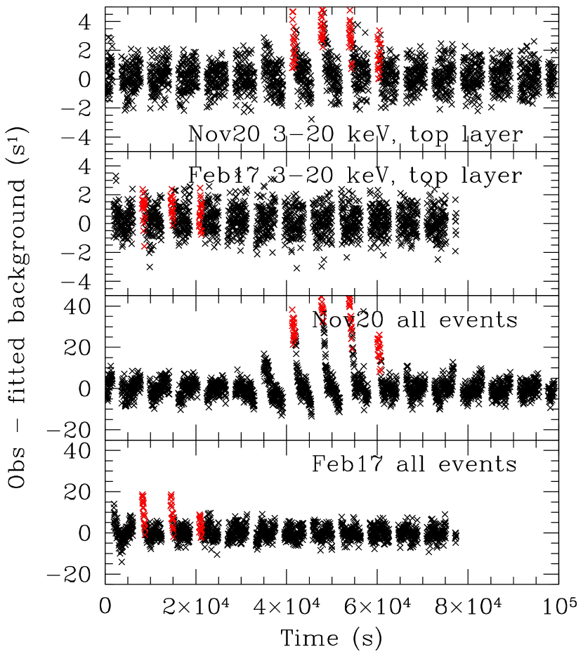
Figure 5: The residuals in the fit to background of LAXPC20 for the two background observations obtained using the improved background model. The left panel shows the residuals in the light curve with a time-bin of 32 s. The red points mark the time interval that is now removed from the GTI. The right panel shows the residuals in the energy spectrum.

Apart from the orbital and quasi-diurnal variation, the LAXPC background also shows some long term variation as shown in Figure 4. This figure shows the average count rate during the background observations corrected for gain shift and quasi-diurnal variation. It can be seen that the background counts in LAXPC20 have increased by about 20% over the last 6 years, but the gradient has reduced since 2019 and the counts are relatively stable during 2020–21. Figure 5 shows the residuals in the background fit to the light curve and the spectrum for two representative background observations. This figure can be compared with Figure 14 of Antia et al. (2021) which shows the results for the same background observations using old background model. It can be seen that there is some improvement in the fit to both the light-curve and the spectrum. It may be noted that the $y$-axis range in the spectrum fit is reduced as compared to that in the old figure due to significant improvement in the fit. Since the typical count rate in LAXPC spectrum is 2 c s^-1 keV^-1, the difference is less than 1% in all cases. For the February 2017 background observation it appears that there was no need to restrict the GTI. This is a special case, while for almost all background observations it is needed to remove some part of GTI. The reason for this is not clear, but out of about 60 background observations only in 3 cases the GTI adjustment may not be needed. For the sake of uniformity we have applied this correction to all observations after 4 April 2016. For earlier observations the GTI correction is not applied. There is only one long background observation during March 2016 in this earlier period.

As described by Jahoda et al. (2006) the detector background is expected to be contributed by (i) the cosmic X-ray background, (ii) charged particle flux in the local environment (iii) induced radioactivity in the spacecraft. Simulation of the detector background (Antia et al., 2017) appears to suggest that the first component is dominant as far as total count rate is concerned. However, the temporal variations are predominantly caused by the other two components. The secular long term variation are likely to be from the induced radioactivity, while the shorter term variations on time-scale of a day or shorter may be from the charged particle flux in the satellite environment. This component is likely to be correlated with the geographic position of the satellite relative to the Earth. As a result, we can expect this variation to show diurnal variation with the period estimated above. In fact, the region with high background count rate in LAXPC is correlated to region where the Charged Particle Monitor (CPM) on board AstroSat (Rao et al., 2017) finds high count rate. The Proportional Counter Array (PCA) on board the Rossi X-ray Timing Explorer (RXTE) also appears to show similar variation (Figure 25 of Jahoda et al., 2006) which has been attributed to the correlation with apogee precession (Jahoda et al., 2006). Similarly, the Large Area Counter (LAC) on board Ginga also shows similar variations (Hayashida et al., 1989). This appears to be similar to what we find in the LAXPC detector. The orbital parameters of Ginga/LAC, RXTE/PCA and AstroSat/LAXPC are quite different. Ginga and RXTE had higher orbital inclination of $31^{\circ}$ and $23^{\circ}$ (Jahoda et al., 1996), respectively, while AstroSat is in near equatorial orbit with an inclination of $6^{\circ}$. The Ginga orbit also had a higher eccentricity with altitude ranging from 517 km to 708 km. Similarly, RXTE altitude ranged from 580 km just after launch to 490 km at the end of operation. While AstroSat altitude is in a narrow range of 630 km to 650 km (Figure 1). AstroSat passes through the northern end of SAA where the charged particle flux is order of magnitude or more lower than that for latitudes of $15^{\circ}$ to $30^{\circ}$, traversed by Ginga and RXTE. As a result, we would expect the induced radioactivity in AstroSat to be much lower than that in Ginga or RXTE. The short term variations in the background rates of LAC, PCA and LAXPC are therefore, expected to show some differences, but the basic features of the background are the same. The short term variations in LAC and PCA have been modelled using induced radioactivity. For LAXPC we have been able to model most of the variation by treating the count rate as a function of latitude and longitude, supplemented by a diurnal variation. The remaining part in a few orbits is discarded from the GTI as that shows a rather large deviation, which has significant variation on long time-scales.

Figure 6: The position of 30 keV peak in the calibration source as a function of time since 20 March 2017, just after the last adjustment of HV. The solid line shows a straight line fit to the data.

Another improvement is made in applying the gain shift to the background spectrum to match that in the source spectrum. This was done using the measurement of gain obtained from the calibration source in veto anode A8. It was found that apart from a steady linear trend the gain also has some fluctuations of the order of 2 channels (out of 1024). If the calculated gain shift is not correct it can introduce some features around 30 keV where there is a prominent peak in the background spectrum due to Xe K florescence. To improve the situation for LAXPC20 data taken after 1 April 2017 (after the last HV adjustment in the detector on 16 March 2017) the gain is fitted to a straight line and gain shift between the background and source spectrum is calculated using this fit. Figure 6 shows the peak position of 30 keV line in LAXPC20 after the last adjustment and the straight line fit to it. The fit gives a variation of 1 channel in the peak position in about 150 days. Since typical separation between the background and source observations is less than one month, it gives a shift of less than 0.2 channels in most cases, which should not introduce any artifact. This measure is not applied to older data and to other two detectors as there the slope of gain change was much larger and adjustment in HV or gas purification were more frequent (figure 2 of Antia et al., 2021).

5 Summary

The LAXPC background shows a prominent quasi-diurnal variation which was not accounted for in the earlier background models. Using over 5 years of data the period of the quasi-diurnal variation is determined to be 84495 s, which is the diurnal variation corrected for the precession of the orbit. Identification of this period also made it possible to identify the orbits where a large deviation was observed just after exit from SAA. After incorporating this period in the background fit and removing some interval from GTI, there is a significant improvement in the background model and this model is incorporated in the latest version of the software.

References

- Agrawal (2006) Agrawal, P. C. 2006, Advances in Space Research, 38, 2989
- Agrawal et al. (2017) Agrawal, P. C., Yadav, J. S., Antia, H. M. et al. 2017, J. Astrophy. Astron., 38, 30
- Antia (2012) Antia, H. M. 2012, “Numerical Methods for Scientists and Engineers”,3rd edition, Hindustan book agency, New Delhi
- Antia et al. (2017) Antia, H. M., Yadav, J. S., Agrawal, P. C., et al. 2017, ApJS, 231, 10
- Antia et al. (2021) Antia, H. M., Agrawal, P. C., Dedhia, D. et al. 2021, J. Astrophys. Astron., 43, 32
- Hayashida et al. (1989) Hayashida, K., Inoue, H., Koyama, K., et al. 1989, PASJ, 41, 373
- Jahoda et al. (1996) Jahoda, K., Swank, J. H., Giles, A. B., et al. 1996, Proc. SPIE 2808: EUV, X-ray and Gamma-Ray Instrumentation for Astronomy VII, eds. Oswald H. Siegmund and Mark A. Gummin, 59
- Jahoda et al. (2006) Jahoda, K., Markwardt, C. B., Radeva, Y., et al. 2006, ApJ, 163, 401
- Misra et al. (2021) Misra, R, Roy, J,, Yadav, J. S., 2021, J. Astrophys. Astron., 42, 55
- Rao et al. (2017) Rao, A. R., Patil, M. H., Bhargava, Y., et al. 2017, J. Astrophy. Astron., 38, 33
- Shaposhinikov et al. (2012) Shaposhnikov, N, Jahoda, K., Markwardt, C., et al. 2012, ApJ, 757, 159
- Yadav et al. (2016) Yadav, J. S., Agrawal, P. C., Antia, H. M., et al. 2016, Proc. SPIE, 9905, 99051D