Machine Learning in Molecular Dynamics Simulations of Biomolecular Systems

Abstract

Machine learning (ML) has emerged as a pervasive tool in science, engineering, and beyond. Its success has also led to several synergies with molecular dynamics (MD) simulations, which we use to identify and characterize the major metastable states of molecular systems. Typically, we aim to determine the relative stabilities of these states and how rapidly they interchange. This information allows mechanistic descriptions of molecular mechanisms, enables a quantitative comparison with experiments, and facilitates their rational design. ML impacts all aspects of MD simulations – from analyzing the data and accelerating sampling to defining more efficient or more accurate simulation models. This chapter focuses on three fundamental problems in MD simulations: accurately parameterizing coarse-grained force fields, sampling thermodynamically stable states, and analyzing the exchange kinetics between those states. In addition, we outline several state-of-the-art neural network architectures and show how they are combined with physics-motivated learning objectives to solve MD-specific problems. Finally, we highlight open questions and challenges in the field and give some perspective on future developments.

Keywords

Molecular dynamics; machine learning; AI4Science; molecular kinetics; protein biophysics

Objectives

• Broadly identify current problems in molecular dynamics simulations of large molecular systems specifically proteins.

• Give a broad overview of machine-learning methods

  • To estimate and analyse model molecular kinetics

  • To sample the Boltzmann distribution

  • To estimate coarse-grained molecular dynamics forcefields

1 Introduction

Molecular dynamics (MD) studies of biomolecular macromolecules, such as proteins, are an invaluable computational tool to study the interplay between structure, function, and dynamics. The conformational flexibility of proteins enables them to be at the center of life itself: with it, they can regulate complex biological processes, such as gene expression (Arber and Linn, 1969; Naveed and Khan, 2001), respond to the environment of the organism (Bezanilla, 2008), or metabolize nutrients to convert them into energy (Fothergill-Gilmore and Michels, 1993; Ude et al., 2021). The dynamics span several orders of magnitude, ranging from side chain rotations and hydrogen bond formation on the pico- and nanosecond timescale to ligand binding, domain movements, and allosterism on the millisecond to second or even minute timescale (Ortega et al., 2013). MD simulations have been central in identifying the mechanism-of-action of these processes at atomic resolution (Sharma et al., 2007; Shaw et al., 2010; Roccatano et al., 2007; Klepeis et al., 2009; Darve et al., 2008). With this enormous expressive power comes a price, however: sampling over a range of timescales also requires long simulation times, resulting in huge amounts of data and no guarantee that the conformational space is sufficiently sampled. Luckily, over the years, there have been many techniques developed to tackle these challenges: longer timescales can be accessed by simulating coarse-grained instead of full-atom systems (Gkeka et al., 2020), sampling can be enhanced with methods such as replica exchange or metadynamics Grubmüller (1995); Laio and Parrinello (2002); Sugita and Okamoto (1999) to overcome the complex energy landscapes with numerous local minima separated by kinetic bottlenecks (Bernardi et al., 2015; Invernizzi et al., 2020), and powerful computational tools that allow for an efficient analysis of the data to extract the relevant kinetic and thermodynamic parameters (Glielmo et al., 2021; Noé, 2020). What connects all of those techniques is that they have a big potential to be combined with recent advances in machine learning (ML) methods. In this chapter, we outline several successful mergers of MD-motivated objectives and various ML techniques (Noé et al., 2020b, a; Wang et al., 2020a). While the repertoire of ML architectures is large and ever expanding, we focus here on approaches with a clear physics and problem-based application in MD.

We expect basic understanding of probability theory, statistical mechanics, and molecular dynamics simulations, and provide a self-contained treatment of relevant ML approaches.

1.1 Molecular dynamics – Key problems

Trajectories obtained by molecular dynamics simulations can be viewed as realizations of a time-discrete Markov process $\mathbf{x}_{t}$ on a continuous state space $\Omega\in\mathbb{R}^{3N}$. That is, the simulation should be set up in a way that the end points of infinitely long simulations follow the equilibrium distribution $\mu(\mathbf{x})$:

$$\lim_{\tau\rightarrow\infty}p_{\tau}(\mathbf{x}|\mathbf{x}_{t-\tau})=\mu(\mathbf{x})\propto\exp\left(-\frac{U(\mathbf{x})}{k_{\text{B}}T}\right),$$ (1)

where $U$ is the potential energy function of the system and $1/k_{\text{B}}T$ is the Boltzmann factor. $p_{\tau}$ is called the transition density. It is a theoretical concept that can be defined using continuous space dynamics. We can view the propagation of probability density in time as

$$\rho_{t+\tau}(\mathbf{x}_{t+\tau}) =\int_{\mathbf{x}_{t}\in\Omega}\rho_{t}(\mathbf{x}_{t})p_{\tau}(\mathbf{x}_{t+\tau}|\mathbf{x}_{t})\,\mathrm{d}\mathbf{x}_{t}$$ (2)

$$=\mathcal{T}\circ\rho_{t}(\mathbf{x}).$$ (3)

Here, $\mathcal{T}$ is the called the ‘Markov operator’ – a mathematical object, that propagates the probability densities on a state space in time. Given some initial distribution $\rho_{t}(\mathbf{x})$ (‘initial condition’) over, for example, the conformational space, applying the Markov operator gives us the corresponding probability density at $t+\tau$, advancing by some time $\tau$. A practical example would be a molecular dynamics simulation from a single molecular configuration, $\mathbf{x}_{0}$, which corresponds to an initial condition $p_{0}(\mathbf{x})=\delta(\mathbf{x}=\mathbf{x}_{0})$, where $\delta$ denotes Dirac’s delta function. Although the initial condition is infinitely narrow, the distribution $p_{0+\tau}(\mathbf{x}_{0+\tau})$ will relax to the Boltzmann distribution for large $\tau$.

A key advantage of using this Markov operator formalism is that it allows us to fully describe the stationary and dynamical processes of molecular systems via its spectral properties – the eigendecomposition Prinz et al. (2011). The leading eigenfunction, with eigenvalue $\lambda_{0}=1$, corresponds to the Boltzmann distribution $\mu(\mathbf{x})$; and all eigenfunctions with $|\lambda_{i}|<1$ – informally – represent how probability ‘flows’ between different parts of state space, on timescales given by the eigenvalues $t_{i}=-\nicefrac{{\tau}}{{\log|\lambda_{i}|}}$ (Fig.1B, C). Approximating these properties of $\mathcal{T}$ remains a key problem in molecular dynamics today.

When we study molecular systems with MD simulations, a common aim is to approximate expectation values. We can express these expectation values in terms of the eigenfunctions and -values of $\mathcal{T}$, thereby directly comparing them to dynamic and stationary experiments, such as free energies of binding or time correlation functions.

Given its comprehensive representation of molecular dynamics, the Markov operator provides the foundation for many learning tasks when applying machine learning to molecular dynamics – either directly or indirectly. These learning tasks seek to identify, quantify, or characterize the following three molecular properties:

• metastable states of a system,

• kinetics of exchange between those states, and the

• thermodynamic populations of the metastable states,

In practice, we achieve these goals by approximating the Markov operator or one of its parts. With Markov state models (MSMs) we try to directly approximate $\mathcal{T}$ via discretization and analysis of large molecular dynamics data sets (see section 2). Analysing the eigenfunctions of $\mathcal{T}$ can help us identify long-lived, or metastable, states using, for example, Perron Cluster Cluster Analysis (PCCA+) (Weber and Kube, 2005; Röblitz and Weber, 2013). Advanced sampling methods (section 3) often rely on prior knowledge of slowly mixing collective variables which correspond eigenfunctions of $\mathcal{T}$ with a large eigenvalues. An effective way to define coarse-grained force fields (section 4) corresponds to integrating out degrees of freedom which do not alter the thermodynamic probabilities of major metastable states.

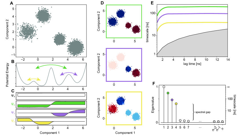
Figure 1: Toy Markov state model and its analysis. A: The data were projected onto the first two components. Four macrostates can be observed. B: 1D potential energy surface. Transitions between the states require high energy and therefore take a long time to be sampled. C: The eigenfunctions of the associated processes $\Psi_{1},...,\Psi_{4}$ are shown. D: The processes can be visualized by analyzing the right eigenvectors of the transition matrix. The respective processes are depicted in the three frames and can be interpreted as transitions between the blue and red states. E: Implied timescale plots of the three processes. The timescale of the respective processes is shown as a function of lag time. All three are well resolved and converge at a lag time of $3$\,\mathrm{n}\mathrm{s}$$. The black line indicates the lag time border. F: Eigenvalue spectrum of the Markov operator; the spectral gap indicates the gap between the timescale of the three slow processes and the timescale of the other processes that are very fast.

2 Modeling molecular kinetics from large MD datasets

Massively parallel molecular dynamics simulations on large high-performance computing (HPC) facilities or cloud computing services have lead to an explosion in the cumulative simulation times in molecular dynamic studies Pande and Shirts (2000). With the increasing volumes of data comes a new challenge: how do we make sense of it? Given the enormous amounts of data, we cannot rely only on visually inspecting the trajectories. The question then becomes, how can we extract quantitative insights from such data sets? Such MD data, are ‘unlabeled.’ In other words: we have all-atom coordinates but no labels, such as, what metastable state each conformer belongs to. Consequently, from a ML perspective, it means we have an ‘unsupervised’ or ‘self-supervised’ problem.

2.1 Markov state models

Markov state models (MSMs) are a popular approach to analyse molecular dynamics simulations, and principle allows us to approximate the properties of the Markov operator, $\mathcal{T}$ (Schütte et al., 1999; Prinz et al., 2011; Bowman et al., 2014; Noé, 2020; Swope et al., 2004; Pande et al., 2010). MSMs allow this approximation since they constitute spatial discretization of $\mathcal{T}$ on a segmented configuration space of disjoint states. Consequently, our ability to predict the properties of interest is limited by how well we discretize the space, and how accurately we can estimate the transition probabilities, $\mathbf{T}$, between the discrete segments of configurational space, from our available data. Akin to the Markov operator formalism, we can then extract predictions of molecular properties from the spectral decomposition of the transition probability matrix $\mathbf{T}$.

Building an MSM typically involves four main steps:

1. Featurization

2. Dimensionality reduction

3. Clustering

4. Estimation of transition matrix.

All of these steps are instances of unsupervised or self-supervised machine learning. The first selects what features of the molecular system – for example, distances, angles, dihedrals, etc. – are important to describe the properties of interest. The second, summarizes these features into a lower-dimensional space. The third step segments the reduced space into discrete segments. The final step estimates the MSM, or transition matrix, $\mathbf{T}$.

In this section, however, we will mainly focus on the last step. Readers who are interested in learning more about the first three steps are referred to the recent review of Glielmo et al.. However, before discussing transition matrix estimation, we informally discuss the MSM as well as its properties and relationship to $\mathcal{T}$.

2.1.1 Markov state models in a nutshell

Consider the system in figure 1. From visual inspection of the stationary density depicted in panel A, we see that there are four metastable states, corresponding to free energy basins (panel B), whose exchange is governed by three eigenvectors (panels C and D). Each of these states might correspond to a specific structural configuration, such as the formation or unfolding of a helix, cis–trans-isomerization, or a binding–unbinding event Olsson (2021); Plattner et al. (2017).

The eigenvalues (panel F) corresponding to the eigenvector, encode the timescales of exchange (panel E), over the free energy barriers (panel B). Note that although we make a fine discretization of the space into $n$ space segments, only four eigenvalues are significantly larger than 0 with a distinct ‘spectral gap.’ Such an eigenvalue spectrum indicates a clear separation of timescales between fast motions (fluctuations within the metastable states) and slow motions (exchange between the metastable states).

The eigenvectors, are the discrete representations of eigenfunctions of $\mathcal{T}$, and have an analogous interpretation. When the value of an eigenvector $\Psi_{i}$ is close to zero, it means that that position in configuration space is unaffected by the exchange process. Conversely, points in configurational space with negative values along $\Psi_{i}$ exchange with positive-valued points along the exchange process (panel C).

2.1.2 Transition probability matrix estimation

To estimate a MSM, the simplest approach is to simply count the transitions between all segment pairs $i$ to $j$, given a lag-time, $\tau$, and organize these counts in a count matrix $\mathbf{C}(\tau)\in\mathbb{N}^{n\times n}$. If we row-normalize – i.e., divide each row in $\mathbf{C}(\tau)$ by its row sum – we obtain a maximum likelihood estimate of the MSM transition matrix. While this approach is intuitively appealing, it is rarely used in practice. The limited use is due to imperfect and finite data which makes estimation unstable. Enforcing a detailed-balance constraint on the estimator is common, to reduce the number of free parameters as is using alternative counting schemes Prinz et al. (2011); Bowman et al. (2014), to ensure robust estimation.

Discretization errors can lead to a lag time, $\tau$, dependence of $t_{i}$, and adjusting $\tau$ to ensure ‘convergence’ is critical when estimating MSMs. MSMs are often validated using the Chapman-Kolmogorov test, where we test for self-consistency:

$$T(k\tau)\approx T^{k}(\tau)$$ (4)

between MSM estimated with a lag time $k\tau$ compared to one estimated with lag time $\tau$ but applied $k$ times to an initial distribution. Due to Markovian dynamics, these should be the same up to a numerical error.

2.1.3 MSM properties

At the heart of Markov state models is the transition matrix $\mathbf{T}$. For $n$ states, we get an $n\times n$ matrix containing the transition probabilities from and to each cluster:

$$\mathbf{T}(\tau)=\begin{bmatrix}p_{ii}&\cdots&p_{in}\\ \vdots&\ddots&\vdots\\ p_{in}&\cdots&p_{nn}\end{bmatrix}.$$ (5)

This matrix is related to the kinetic rate matrix $\mathbf{K}$ by

$$\mathbf{T}(\tau)=\exp(-\mathbf{K}\tau)$$ (6)

in units per time, where $\exp(\cdot)$ here refers to the matrix exponential. Now we will show how the eigenvectors and -values of $\mathbf{T}$ and $\mathbf{K}$ reveal the connection between transition probabilities and relaxation timescales.

The eigenvectors (and eigenvalues) can be obtained via eigendecomposition of the transition matrix (equation 5)

$$\mathbf{T}(\tau)=\mathbf{L}\boldsymbol{\Lambda}(\tau)\mathbf{R},$$ (7)

where $\mathbf{L}$ and $\mathbf{R}$ are the orthonormal left and right eigenvectors, respectively. $\boldsymbol{\Lambda}(\tau)$ denotes the diagonal matrix containing the eigenvalues. The left eigenvectors are equal to the right eigenvectors weighted by the stationary density, $\mu(\mathbf{x})$.

In figure 1B we show the three slowest processes of our model system corresponding to the the right eigenvectors, $\Psi$, (1C).

From linear algebra, we know that the eigenvectors of $\mathbf{T}$ and $\mathbf{K}$ are the same, implying that the processes do not change when converting the transition matrix to the kinetic rate matrix. The eigenvalues of the transition matrix are linked to the ‘implied’ timescales in the following way:

$$t_{i}=-\frac{\tau}{\log|\lambda_{i}|},$$ (8)

where $t_{i}$ correspond to the timescale of the process $\Psi_{i}$ (figure 1C), we see that there are only a few that are close to 1 (figure 1F).

2.2 Variational methods for estimating conformational dynamics

While MSMs are a broadly used method to analyse large volumes of MD data, it is a special case of more fundamentally motivated variational principles. These variational principles allow us to compute the eigenvalues and -vectors in an arbitrary set of basis functions, and not just on a discrete state space, as with MSMs. The first is the variational approach to conformational dynamics (VAC) and was proposed by Noé and Nüske (2013) and Nüske et al. (2014).

The eigenfunctions and eigenvalues of a dynamical system fulfilling detailed balance

$$\mu(\mathbf{x})p_{\tau}(\mathbf{y}\mid\mathbf{x})=\mu(\mathbf{y})p_{\tau}(\mathbf{x}\mid\mathbf{y})$$ (9)

with a unique stationary distribution $\mu(\mathbf{x})$, are related to the Markov operator $\mathcal{T}$ in the following way:

$$\mathcal{T}(\tau)\Psi_{i}=\lambda_{i}\Psi_{i},$$ (10)

where $i$ is an eigenvalue/-function pair. The VAC strategy is to approximate the dominant eigenvalues $\lambda$ and -functions $\Psi$ in a manner similar to that of the Rayleigh-Ritz variational principle from quantum mechanics (Gross et al., 1988). The eigenfunction of a dynamical process can be approximated by superimposing feature functions:

$$\hat{\Psi}_{i}=\hat{\mathbf{v}}_{i}^{\top}\chi(\mathbf{x}_{t})$$ (11)

where $\chi(\mathbf{x}_{t})$ is a feature transformation and $\hat{\mathbf{v}}$ are the eigenvectors we want to find. In other words, VAC allows us to find an approximation of the eigenfunction $\hat{\Psi}_{i}$ as a linear combination of vector features, $\chi(\cdot)$.

Markov state models are a special case of the VAC principle — if we choose our feature function to be the indicator function: $\chi(\mathbf{x})$ is 1 when $\mathbf{x}$ is in the $i$th cluster and 0 otherwise). Approximating the Markov operator $\mathcal{T}$ then gives us an estimate of the transition matrix of a Markov state model (section 2.1):

$$\hat{\mathbf{T}}(\tau)=\underbrace{\boldsymbol{\Sigma}_{00}^{-1}}_{\begin{subarray}{c}\text{instantaneous}\\ \text{covariances}\end{subarray}}\underbrace{\boldsymbol{\Sigma}_{0\tau}}_{\begin{subarray}{c}\text{time-lagged}\\ \text{covariances}\end{subarray}}$$ (12)

where we make use of two of the three covariance matrices

$$\boldsymbol{\Sigma}_{00} =\frac{1}{t}\sum_{t=1}^{t-\tau}\chi(\mathbf{x}_{t})\chi(\mathbf{x}_{t})^{\top}$$ (13)

$$\boldsymbol{\Sigma}_{0\tau} =\frac{1}{t}\sum_{t=1}^{t-\tau}\chi(\mathbf{x}_{t})\chi(\mathbf{x}_{t+\tau})^{\top}$$ (14)

$$\boldsymbol{\Sigma}_{\tau\tau} =\frac{1}{t}\sum_{t=1}^{t-\tau}\chi(\mathbf{x}_{t+\tau})\chi(\mathbf{x}_{t+\tau})^{\top}.$$ (15)

Using eigendecomposition of $\hat{\mathbf{T}}(\tau)$, we can obtain an estimate of the eigenvalues $\hat{\lambda}_{i}$. The variationally optimal solution will be the $\hat{\lambda}_{i}$ with the highest variational score $\mathcal{L}_{\text{VAC}}$:

$$\mathcal{L}_{\text{VAC}}\equiv\sum_{i=1}^{k}\hat{\lambda}_{i}\leq\sum_{i=1}^{k}\lambda_{i}.$$ (16)

Equation 16 tells us that the estimated eigenvalues $\hat{\lambda}$ always underestimate the true eigenvalues $\lambda$ (the estimate will be exact only if $\hat{\lambda}=\lambda$). We can optimize this upper bound by maximizing the $k$ largest eigenfunctions of our estimate in equation 12. That is, we vary a set of vectors until we obtain the maximum in expression 12. The solution we obtain will vary depending on our choice of feature functions. In fact, we can use 16 to parameterize deep neural networks or kernel models (Chen et al., 2019).

A method that is similar to the VAC approach is (extended) dynamic mode decomposition (DMD) (Mezić, 2005; Rowley et al., 2009; Schmid, 2010; Williams et al., 2015). DMD also attempts to identify slow collective variables. Contrary to VAC, however, DMD uses regression to approximate the left eigenvectors of the dynamical system instead of the eigenfunctions (Koopman, 1931; Koopman and v. Neumann, 1932; Williams et al., 2015). That is, for a time series $\{\mathbf{X}_{t}\}$, we are trying to minimize $||\mathbf{X}_{t+\tau}-\mathbf{DX}_{t}||_{F}$ with $F$ being the Frobenius norm. Dynamic mode decomposition identifies the linear operator $\mathbf{D}$ and computes its eigenvectors and the respective largest eigenvalues. The solution of DMD and VAC, i.e., the eigenvectors which constitute the collective variables, hence are the same for the same set of basis functions (Klus et al., 2018).

2.2.1 Time-lagged independent component analysis (tICA) as method for learning slow collective variables and dimensionality reduction

We can exploit the time dependence of MD data not only to establish kinetic models but also in the context of dimensionality reduction. Similar techniques were first described in electrical engineering to separate mixtures of independent signals (Molgedey and Schuster, 1994) but the principle is the same. We can calculate the covariance matrix $\boldsymbol{\Sigma}_{00}$ and the time covariance matrix $\boldsymbol{\Sigma}_{0\tau}$ at lag time $\tau$ (equations 15) (Pérez-Hernández et al., 2013). Similar to principal component analysis (see info box 2.4.1), we can define a generalized eigenvalue problem as

$$\boldsymbol{\Sigma}_{0\tau}\mathbf{V}=\boldsymbol{\Sigma}_{00}\mathbf{V}\boldsymbol{\Lambda},$$ (17)

where $\boldsymbol{\Lambda}$ is a diagonal matrix containing the eigenvalues in the diagonal. However contrary to PCA, the eigenvector $\mathbf{v}_{i}$ in $\mathbf{V}$ characterizes the component with maximal autocorrelation (instead of maximal variance), that is $\mathbb{E}[\mathbf{v}_{i}(\mathbf{X}_{t})\mathbf{v}_{i}(\mathbf{X}_{t+\tau})]$. Here we also see the close relationship between tICA and MSMs. Equation 17 is the problem we have already encountered in section 2.2, where we showed that MSMs are a special case of the variational approach to molecular kinetics. tICA is also a special case in that $\boldsymbol{\Sigma}_{0\tau}$ is symmetric. Contrary to MSMs, the basis set used in tICA is not a one-hot encoding but instead linear basis functions applied to the data. Importantly, the eigenvalues of equation 17 contained in $\boldsymbol{\Lambda}$ also reflect the relaxation timescales (see chapter 2.1). Similar to PCA, truncation of $\mathbf{V}$ after the slowest $d$ independent components enables the use of tICA as a dimensionality reduction method. Time-lagged independent component analysis also only works for linear manifolds. However, there have been approaches introduced that make use of kernel methods to deal with non-linear data manifolds (Noé and Nüske, 2013). These have a number of drawbacks, however. On the one hand, they have a high computational cost and on the other, they are extremely sensitive to the hyperparameters and need extensive tuning (Harrigan and Pande, 2017). Due to its double role as, both, a dimensionality reduction method as well as a kinetic model, tICA is the central method employed as a preprocessing method for establishing a Markov state model.

2.3 Variational approach to Markov processes (VAMP)

When estimating the conformational dynamics of a system, we cannot always assume the system is in equilibrium. That includes situations in which the system experiences, for example, concentration or temperature gradients. In non-equilibrium cases, the variational approach to Markov processes (VAMP) (Wu and Noé, 2020) provides a generalization of VAC (see section 2.2). VAMP does not require the detailed balance condition (equation 9). As a consequence, the time-lagged covariance (for MSMs, the count matrix, equation 14) is not symmetric. This assymmetry leads to the complex-valued eigenvalues of for example, the transition matrix, making variation optimization using VAC difficult without further assumptions. VAMP instead uses singular value decomposition of a matrix computed from the feature covariances (equations 13-15) to solve a more general variational problem. In contrast to VAC, VAMP maximizes a score which depends on the singular values of the estimated dynamical model (Noé and Clementi, 2015; Wu and Noé, 2020) (See example, Sec 2.4). While conceptually similar, the singular values cannot be related back to the implied time-scales, unlike the eigenvalues.

2.4 Neural network approaches for identification of reaction coordinates

Deep learning in particular has shown to be extremely powerful due to its ability to approximate complex non-linear functions (Lecun et al., 2015). This potential has also been recognized in the MD community, and hence, many approaches have been developed to analyze the kinetics of molecular systems and to identify reaction coordinates. Here, we will briefly go through the most recent advances in identifying slow collective variables from molecular simulations data using neural networks.

In section 2.1, we saw that in order to build a Markov model, a number of manual steps have to be performed in order to obtain transition matrix $\mathbf{T}$: featurization, dimensionality reduction, clustering, and finally estimation of the transition matrix. In principle, these are all steps that can be performed in an end-to-end framework (Mardt et al., 2018). The VAMP approach (section 2.3) can be used to train deep neural networks: VAMPnets replace all steps mentioned above by training a neural network that learns a feature space encoding of the dominant eigenfunctions $\Psi$. Figure 2 shows a schematic representation of the neural network architecture. The input consists of two parts: the coordinates of the trajectory at each time step $t$ and $t+\tau$. The inputs are then passed through the neural network, and we obtain a feature set, $\chi_{0}(\mathbf{x}_{t})$ and $\chi_{1}(\mathbf{x}_{t+\tau})$, that is optimized via the VAMP score: Using the covariance matrices in equations 13-15, we get

$$\mathcal{L}(\chi_{0},\chi_{1})=\Big{|}\Big{|}\boldsymbol{\Sigma}_{00}^{-\frac{1}{2}}\boldsymbol{\Sigma}_{0\tau}\boldsymbol{\Sigma}_{\tau\tau}^{-\frac{1}{2}}\Big{|}\Big{|}_{F},$$ (18)

Aside from the variationally optimized latent space representations, we also obtain a Koopman model $\mathbf{T^{\prime}}(\tau)$ as an output. This matrix, however, is not necessarily a valid stochastic matrix. The entries of $\mathbf{T^{\prime}}(\tau)$ can therefore not be interpreted as transition probabilities. In addition, even systems that have been simulated in equilibrium are not guaranteed to have a reversible kinetic model. An extension of the original algorithm allows for the incorporation of physical constraints, such as reversibility or avoiding non-negative entries, such that the Koopman model obtained can be interpreted as a transition matrix (Mardt et al., 2019). This extension also outlines an approach for experimental data integration. Deep generative MSMs (DeepGenMSMs) have been developed by extending the VAMPnet architecture that includes a generator that samples novel time-lagged configurations that the model has not seen in the training data (Wu et al., 2018).

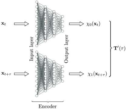
Figure 2: Neural network architecture of VAMPnets. The network consists of two lobes that take the data $\mathbf{x}_{t}$ and $\mathbf{x}_{t+\tau}$ as inputs to find a lower-dimensional representation $\chi_{0}(\mathbf{x}_{t})$ and $\chi_{1}(\mathbf{x}_{t+\tau})$, respectively. During training, the variational score is maximized. The output is a Koopman model that assigns probabilities to the $n$ states. Introducing physical constraints to the model, it is then possible to interpret the output as a valid transition matrix.

An alternative approach to identify slow collective variables is by using an autoencoder that learns a lower-dimensional representation of time-lagged data and then predicts later time frames using regression Wehmeyer and Noé (2018). The loss function of this time-lagged autoencoder (TAE) is

$$\mathcal{L}_{\text{TAE}}(q_{\phi},p_{\theta};\mathbf{x})=\min_{p_{\theta},q_{\phi}}\sum_{t}||\mathbf{x}_{t+\tau}-p_{\theta}(q_{\phi}(\mathbf{x}_{t}))||^{2},$$ (19)

$q_{\phi}$ and $p_{\theta}$ are the encoding and decoding nets of the neural network, respectively. Recall, neural networks are particularly well suited to learn non-linear feature transformations. This property is particular useful in cases where metastable states may be not linearly separable in the input features. As such, TAEs can be seen as a non-linear extension of TICA. At first sight, TAEs are closely related to VAMPNets or DeepGenMSMs (Wu et al., 2018), and indeed, the architectures mainly differ by the lack of a decoder network in VAMPnets. This means that TAEs not only learn a feature encoding but also a decoding of the features to the full configurational space. The main limitations of TAEs compared to VAMPnets or DeepGenMSMs are, however, that TAEs lack the ability to sample from the transition density $p$, i.e., $\mathbf{x}_{t+\tau}\sim p_{\tau}(\mathbf{x}_{t+\tau}|\mathbf{x}_{t})$.

2.4.1 Long short-term memory neural networks for learning molecular dynamics

Capturing the temporal dependence in molecular dynamics simulations of biomolecular trajectories is crucial in identifying the underlying kinetics and thermodynamics. A popular class of ML algorithms that are widely used in speech recognition or natural language processing (Graves et al., 2013; Cho et al., 2014) are recurrent neural networks (RNNs). RNNs have been extensively applied to protein and DNA sequences, due to their similarity to natural text. However, the application of RNNs to study molecular dynamics, which also has a natural sequential nature, is more limited. Tsai et al. (2020) proposed a method to capture kinetics over several timescales using an long short-term memory (LSTM)(Hochreiter and Schmidhuber, 1997) RNN architecture originally developed for modelling languages. Using gating nodes, the model can capture slow kinetics between metastable states while retaining the memory of previous states. Conceptually, this is similar to an actual gate that controls which information to pass through and which to block, such that the model only retains the relevant information to make predictions and forgets about the information that is irrelevant for modelling the dynamics. Using this mechanism, the model can accumulate information over the course of the trajectory relaxing the Markov assumption made in MSMs. Compared to MSMs, LSTM models are much more complex, potentially making it hard for the model to make reliable predictions. However, estimation of MSMs requires choosing a fixed lag time, that, depending on the choice, can lead to non-Markovian behavior or loss of temporal precision. Since LSTMs are not constrained by the Markovianity assumption, the number of states and lag time do not have to be fixed (although hyperparameter tuning is comparable to choosing the number of states in a hidden Markov model).

2.5 Dynamic graphical models

Characterizing the number of states a biological macromolecule has as well as their exchange rates is at the heart of kinetics studies. As we have seen in section 2.1, Markov state models assign each configuration to a global state with different metastable substates with a characteristic relaxation time. Since the number of possible states grows exponentially with increasing system size, analyzing the dynamics of biomolecular macromolecules with highly frustrated and complex energy landscapes becomes difficult. The dynamic graphical models (DGM) approach (Olsson and Noé, 2019) shifts the paradigm of characterizing dynamics from a global perspective towards viewing macromolecules as systems with many local but coupled subsystems. Here, “local” can mean on a single amino acid or entire domain level, depending on the system. When learning local models, we either have to learn a graph structure (Ravikumar et al., 2010) as is done directly in DGMs Olsson and Noé (2019) or we can assume sub-system independence Hempel et al. (2021). Earlier work proposed a framework to model the temporal causality of several binary random variables, hence investigating the time dependence of subsystems switching between two states (Gerber and Horenko, 2014). DGMs, in contrast, model $q$ state sub-systems, as solving an inverse kinetic Ising-type model problem: we learn the couplings between the sub-systems (spins) (Ising, 1925; Glauber, 1963) and assume Markovian dynamics. Counterintuitively at first thought, by breaking down the dynamics of a system from a global perspective to an (arbitrarily) large number of subsystems, we make the problem of modelling the dynamics tractable: DGMs’ parameter count scales quadratically with the number of sub-systems, whereas MSMs scale exponentially in the number of states. The identification of weakly coupled, decomposable subsystems is a non-trivial task Mardt et al. (2022). More generally, using the VAMP scores introduced in section 2.4, we can evaluate the quality of the decomposition in a Markov state model while retaining the description of a global kinetic model (Hempel et al., 2021). Importantly, with this description, we need not observe all combinations of the different states in order to characterize the global system. In fact, it is even possible to generate new, previously unobserved configurations, allowing for applications in adaptive simulation settings Olsson and Noé (2019). Current limitations of this approach include the integration of experimental observables, which is not as straightforward as with the MSM approachOlsson et al. (2017). Further, direct calculation of global state dynamics, such as its eigenvectors and eigenvalues, is only practical for a few limiting cases: small systems or independent sub-systems.

3 Sampling the Boltzmann distribution

One of the most challenging but also relevant physicochemical parameters to compute is the thermodynamic free energy. It relates the geometric structure of a system to its probability at equilibrium. Typically, structural configurations which exchange on a fast timescale are grouped together into ‘metastable’ states, and the free energy of such a state $A$ is then given by

$$U_{A}=-k_{\text{B}}T\log\left(\int_{\mathbf{x}\in A}\mu(\mathbf{x})\,\mathrm{d}\mathbf{x}\right).$$ (23)

Computing the free energies helps us characterize important features of molecular systems including the binding affinity between two proteins or a protein and a pharmaceutical: the free energy difference between bound and unbound states. Practically, computing free energies corresponds to evaluating an integral of the Boltzmann distribution over segments of the configurational space (equation 23), which is generally intractable analytically. Above we saw how some kinetic models give direct access to state probabilities, and therefore also free energies. In this section, we focus on the efforts into developing sampling methods to characterize the free energy surface, ultimately getting access to the aforementioned information, via Monte Carlo approximations.

In machine learning, sampling from a probability distribution belongs to the field of ‘generative modeling’ (Goodfellow et al., 2016). Other machine learning approaches also play a significant impact on enhanced sampling approaches. For example using unsupervised and self-supervised learning strategies to discover reaction coordinates (see section 2.4) for use with methods such as meta-dynamics, flooding, or umbrella sampling Laio and Parrinello (2002); Grubmüller (1995); Torrie and Valleau (1977). These strategies also contribute to sampling free energy landscapes, yet, we here focus on generative approaches, how they differ, and what their respective advantages and drawbacks are.

3.1 Boltzmann Generators

Most biologically interesting systems have many metastable states and high energy barriers between them. Such a free energy landscape leads to highly peaked Boltzmann distribution, with low-probability regions separating the metastable states. Consequently, simulation-based approaches which do small steps in configuration space, for example as in MD simulations, based on the atomic forces, rarely cross between metastable states. Yet sampling these transitions is critical to accurately estimate free energy changes. Ultimately, the goal is to draw statistically independent samples from the Boltzmann distribution as it allows the convergence of Monte Carlo estimates of equation 23. However, as mentioned, such a task is intractable for a general molecular system in equilibrium and therefore remains a long-standing challenge.

Boltzmann Generators (BGs) (Noé et al., 2019) is a strategy to train normalizing flow models (see box 3.1) to tackle this problem. Briefly, we learn a probability distribution $\rho_{\boldsymbol{\theta}}(\mathbf{x})$ of a configuration space which approximates the Boltzmann distribution $\mu(\mathbf{x})$ using a set of parameters $\boldsymbol{\theta}$. We call $\rho_{\boldsymbol{\theta}}$ a ‘surrogate model’ of the the Boltzmann distribution. The key idea of BGs is that drawing independent statistical samples from the surrogate model is fast and efficient; and we can evaluate the probability of every generated sample at low computational cost. After training such a model, we can then generate samples from $\rho_{\boldsymbol{\theta}}(\mathbf{x})$ to approximate direct sampling from $\mu(\mathbf{x})$. Since we can evaluate the exact likelihood of every sample generated from $\rho_{\boldsymbol{\theta}}(\mathbf{x})$ we can reweigh samples to the Boltzmann distribution using importance sampling Noé et al. (2019), through the unnormalized importance weights

$$\omega_{i}\propto\frac{\exp\left(-\nicefrac{{U(\mathbf{x}_{i})}}{{k_{B}T}}\right)}{\rho_{\boldsymbol{\theta}}(\mathbf{x}_{i})}\hskip 5.69046pt\mathrm{for}\hskip 2.84544pt\mathbf{x}_{i}\sim\rho_{\boldsymbol{\theta}}.$$ (24)

If $\rho_{\boldsymbol{\theta}}(\mathbf{x})$ is a good surrogate of $\mu(\mathbf{x})$, the computed importance weights $\omega_{i}$ for every sample $\mathbf{x}_{i}$ from $\rho_{\boldsymbol{\theta}}(\mathbf{x})$, will all be approximately equal. We can use this importance sampling approach to compute free energy changes or evaluate expectation values over the configuration space – for example experimental observables.

Since normalizing flows build on invertible neural networks (see box 3.1), we can transform molecular configurations into a ‘latent space’ and interpolate between them in that space, and transform intermediate points in latent space back to configuration space. Such an approach allows us to characterize low-energy paths between metastable states. More generally, BGs allow to more efficiently sample and explore the configuration space of molecular systems.

The main innovation of BGs compared to regular normalizing flows lies in the way they are trained. Training is comprised of two parts: “training by example” and “training by energy.” The former is common way training normalizing flow, by maximizing the likelihood of generating samples seen examples. In the context of BGs, examples could include known protein structures in different states, either experimentally obtained or from short MD trajectories. The latter approach is usually not possible. When training BGs, we match the surrogate model $\rho_{\boldsymbol{\theta}}(\mathbf{x})$ and the Boltzmann distribution, using the Kullback-Liebler divergence (Kullback and Leibler, 1951). This latter step is performed by generating samples $\mathbf{x}_{i}$ from $\theta_{\boldsymbol{\theta}}$ and then minimize the expected unit-less potential energy $\nicefrac{{U(\mathbf{x}_{i})}}{{k_{\text{B}}T}}$ where $U(\mathbf{x})$ is a classic force field model as used in MD simulations.

Recent studies show using molecular forces during training (Köhler et al., 2021) or alternative training strategies (Midgley et al., 2021) can potentially improve performance of estimated BGs.

In contrast to enhanced sampling techniques (Sec. 3.2), Boltzmann generators generally do not have to rely on any predefined reaction coordinates (low-dimensional projection of the high-dimensional space), although the information can be used during training.

However, currently BGs lack of transferability, requiring re-training for each individual system. Similarly, dealing with many common simulation settings such as periodic boundary conditions, chemical reactions, or external driving forces is not currently possible. In addition, we note that, depending on the system, it is possible that not all states are visited during training, and BGs would thus have to be combined with other methods, such as MD or MCMC.

Initial works towards transferrable BGs build on including physical symmetries in to the normalizing flows (Köhler et al., 2019; Satorras et al., 2021). While BGs are still their infancy as a technology, they provide a promising new method to efficiently sample the configuration space of proteins and many-body systems in general.

3.2 Enhanced sampling methods

Another approach to overcome the long simulation times required to sample relevant configurations on the relevant timescales is “enhanced sampling.”

Broadly, these methods work by introducing two components: a collective variable (CV) or reaction coordinate (RC) and a biasing potential. Once a CV is defined, one or more simulations are run subject to biasing potentials defined on the CV to encourage ‘mixing’ along it. A more formal and extensive discussion of enhanced sampling methods is beyond the scope of this text, the interested readers are pointed to the excellent review by Hénin et al. (2022). Further, discussing the use of AI and ML methods to inform transition path sampling is also beyond the scope of this text (Jung et al., 2019; Dellago and Bolhuis, 2009).

There are ‘ad hoc,’ and more principled ways of defining CVs; we here focus on the latter which we can use to define a learning objective for ML methods.

The goal of enhanced sampling methods is to facilitate transitions between the free energy minima (metastable states). We have already discussed the eigenfunctions of the Markov operator as slowly relaxing degrees of freedom (Sec. 2), often interconnecting metastable states. Indeed, methods such as VAC, tICA and the related SGOOP (spectral gap optimization of parameters) Tiwary and Berne (2016) serve as basic building blocks for several enhanced sampling methods (McCarty and Parrinello, 2017; Sultan and Pande, 2017; Zou et al., 2021).

Alternatively, Ribeiro et al. and others Bonati et al. (2021) have sought to integrate the sampling and CV discovery more tightly. For example, in their work, Ribeiro et al. (2018) they propose an iterative machine learning–molecular dynamics approach that learns a CV using a variational autoencoder (VAE) (see box 3.2). First, a short unbiased simulation is run. Next, the data are projected to a latent space using the VAE, and Kullback-Leibler divergence is used to pick out a trail CV from a set $\chi_{i}\in\boldsymbol{\chi}$ of candidate CVs. Finally, the latent space distribution and the selected $\chi_{i}$ is used to define a biasing potential, to run a new biased simulation. The procedure is repeated until a convergence criterion is met. A key advantage of this method compared to other related methods (Chen and Ferguson, 2018; Husic and Pande, 2018), is that it uses the expressive power of deep neural networks, yet resulting in an interpretable collective variable.

The neural networks–based variationally enhanced sampling method (Bonati et al., 2019) provides a different strategy: After identifying the collective variables of a system, a bias potential is then introduced to enhance sampling. Here, the authors express the bias as a neural network, ensuring its continuity and differentiability. The network is optimized according to the variational principle introduced in (Valsson and Parrinello, 2014).

Smooth and nonlinear data-driven collective variables (SandCV) (Hashemian et al., 2013) represents a geometry-based approach that can be used for exploring poorly sampled regions in the conformational space. The technique uses isomap Tenenbaum et al. (2000), a multi-dimensional scaling method for dimensionality reduction. The data manifold is then parametrized with maximum entropy basis functions, which can be passed on to enhanced sampling methods, such as the adaptive biasing force method (Darve et al., 2008).

4 Force field parameterization of coarse-grained simulations

All-atom molecular dynamics simulations is the only method which simultaneously grants access to the full spatial and temporal resolution of molecular systems. As we discussed above, given sufficiently accurate and well-sampled data sets, we can use these approaches to gain detailed insights into the kinetics and thermodynamics of any molecular system. However, these simulations remain computationally expensive, and remain inaccurate, despite all the recent advances outlined above as well as improvements in classical MD simulation force field models.

In this section, we discuss how ML is used to parameterize coarse-grained (CG) force fields. We recognize the active field of all-atom force field parameterization enabled by advanced ML method but discussion of these is beyond the scope of this text (Chmiela et al., 2018; Wang et al., 2020b; Unke et al., 2021; Behler and Parrinello, 2007; Käser and Meuwly, 2022; Thölke and Fabritiis, 2022; Hedelius et al., 2022; Smith et al., 2017).

The CG approach goes beyond the Born-Oppenheimer approximation invoked to parameterize classical force fields models. Instead of marginalizing only electronic degrees of freedom, atoms are grouped in to effective beads, lowering the complexity of simulations dramatically. However, the grouping of atoms need to be done in a manner which preserves the important thermodynamic parameters of the all-atom system (Noid et al., 2008). Several CG models exist which achieve this to some extent Souza et al. (2021) – however, new representation learning methods are emerging as an exciting new area of research to build a next-generation family of CG models Husic et al. (2020).

The key idea of CG is to marginalize over – integrate out – the degrees of freedom in an all-atom system which are not important to reproduce the macroscopic properties of interest. We define a probability density of the CG representation, $\mathbf{y}$, as

$$p(\mathbf{y})=\frac{\int\hat{\mu}(\mathbf{x})\delta(\mathbf{y}-M(\mathbf{x}))\,\mathrm{d}\mathbf{x}}{\int\hat{\mu}(\mathbf{x})\,\mathrm{d}\mathbf{x}},$$ (27)

where $\hat{\mu}(\mathbf{x})$ is the unnormalized Boltzmann weight of an all-atom configuration $\mathbf{x}$, and the mapping function $M$ which maps the all-atom coordinates to the corresponding coarse-grained coordinates $\mathbf{y}$. The integral (eq.27) is defined for purely formal reasons; it is generally intractable. Note the similarity to the metastable state free energy (eq.23). Indeed we can express a CG free energy model:

$$U(\mathbf{y})=-k_{\text{B}}T\log\left(p(\mathbf{y})\right)+\text{const}.$$ (28)

In this setting we can identify two learning problems:

• learning the mapping function, i.e., for a system with the configuration $\mathbf{x}\in\mathbb{R}^{3N}\rightarrow\mathbf{y}\in\mathbb{R}^{3n}=M(\mathbf{x})$ with $n<N$.

• learning the free energy model of the coarse-grained representation $\hat{U}(\mathbf{y};\boldsymbol{\theta})$ with parameters $\boldsymbol{\theta}$.

Learning the free energy model is strictly dependent on the a specified map function – conversely, specifying the map is independent of the estimated free energy model (Shell, 2008). In practice, learning $\hat{U}(\mathbf{y};\boldsymbol{\theta})$ has received the most attention with three different estimation strategies: iterative Boltzmann inversion (Lyubartsev and Laaksonen, 1995; McGreevy and Pusztai, 1988), relative entropy minimization (Shell, 2008), flow-matching Köhler et al. (2022), and force matching (Noid et al., 2008; Izvekov and Voth, 2005; Ercolessi and Adams, 1994). Force matching has theoretical connections to score matching in machine learning Hyvärinen (2005) and generalized Yvon-Born-Green theory Mechelke and Habeck (2013); Mullinax and Noid (2010).

Recently, ML-based CG free energy models were trained using the force-matching approach (Husic et al., 2020; Wang et al., 2019b). Force matching is attractive as it may yield a thermodynamically consistent CG free energy model Izvekov and Voth (2005), and we use it as an example of how we can train ML models using principles from CG theory.

In force matching, we try to learn a free energy model $\hat{U}(\mathbf{y};\boldsymbol{\theta})$, such that its forces $-\nabla_{\mathbf{y}}\hat{U}(\mathbf{y};\theta)$ on the CG beads $\mathbf{y}$ match the mapped forces expected from all-atom forces $\mathcal{F}(\mathbf{y})=M_{F}(-\nabla_{\mathbf{x}}U(\mathbf{x}))$, where $M_{F}$ is function which maps forces in a manner consistent with a mapping function $M$ (Ciccotti et al., 2007). Such a procedure requires us to run a reference all-atom simulation, saving both positions and forces at regular intervals, leading to a total of $Q$ snapshots. To train $\hat{U}(\mathbf{y};\boldsymbol{\theta})$ we minimize the squared error between the mean forces and the predicted forces, for all snapshots and CG beads $N$,

$$\mathcal{L}(\mathbf{X};\boldsymbol{\theta})=\frac{1}{3QN}\sum_{i=1}^{Q}||\underbrace{\mathcal{F}(\mathbf{y}_{i})}_{\text{``mapped'' forces}}-\underbrace{\left(-\nabla_{\mathbf{y}_{i}}\hat{U}(\mathbf{y}_{i};\boldsymbol{\theta})\right)}_{\text{predicted CG forces}}||^{2}.$$ (29)

In other words, we have a supervised learning problem, where we have input (coarse-grained coordinates) which we use to predict the labels (coarse-grained forces). Since $U(\mathbf{y})$ is a complex function of multi-body interactions between the CG beads, deep neural networks provide a great ‘ansatz’ to approximate it. Note, in order to optimize the loss (eq. 29) via gradient-based optimization, we need our model $U(\mathbf{y};\boldsymbol{\theta})$ to be differentiable at least two times. Furthermore, we expect a molecular system’s free energy to be invariant to global rotations and translation. Consequently, introducing a featurization layer in our neural network model, where we compute invariant features: distances, angles, and torsions, and use these features as input for a deep neural network (Wang et al., 2019b).

The approach outline above is the basis for CGNets (Wang et al., 2019a), a neural network structure that was introduced to learn coarse graining force fields. Wang et al. also introduced regularized CGNets that add a baseline energy term to avoid physically unrealistic predictions – e.g., overlapping beads. This is a common strategy in the training of neural networks to reduce the generalization error (Goodfellow et al., 2016). The authors show, however, that the outcome of the model is highly sensitive to different hyperparameters, requiring fine tuning for every system individually. In addition, the approach is limited to predicting thermodynamics, kinetics cannot be reliably predicted, and as of yet, a new CG force field needs to be estimated for every system of interest. Nevertheless, the approach is successful, and indeed manages to capture multi-body interactions (Wang et al., 2021).

Kernel-based ML methods provide an alternative strategy to learn CG Free energy models and have also proven successful in reproducing multi-body distribution functions Scherer et al. (2020); John and Csányi (2017).

Husic et al. introduces CGSchnet by integrating a graph neural network (see box 4.1) (Schütt et al., 2018) into the CGnet approach Wang et al. (2019b). In CGSchnet coarse-grain beads are nodes which are initialized with bead-specific features. Over several convolutional layers the beads exchange their feature representations in a distance dependent manner via learned filters Schütt et al. (2018). The learned filters map distances onto radial basis functions – a number of Gaussians placed at regular intervals, which in turn determines how the node feature from bead $i$ gets transmitted to bead $j$. In principle, such a construction could enable a transferable CG potential, as the learned filters are shared between bead types.

CGSchNet broadly outperforms its predecessor in terms of accuracy when predicting the free energy surface; it is also less sensitive to hyperparameters and requires less regularization.

Recently, spectral matching was introduced as a technique to retain the kinetic properties of the system during coarse graining (Nüske et al., 2019), which requires estimating the eigenfunctions and -values of the atomistic system (see chapter 2).

4.1 Learning the mapping function – and recovering all-atom coordinates

The CG mapping function has undergone extensive theoretical analysis (Foley et al., 2015; Shell, 2008; Menichetti et al., 2021; Giulini et al., 2020), yet learning the mapping function remains poorly explored, with recent contributions relying on hand-crafted mapping functions Wang et al. (2019b); Husic et al. (2020).

Two recent machine learning-based methods aim to learn CG mappings. Deep supervised graph partitioning model (DSGPM) (Li et al., 2020), aims to reproduce expert mappings in small molecules by adopting a graph-partitioning approach. Another approach, uses an autoencoder-inspired strategy to learn a mapping function as well as a coarse-grained free energy model simultaneously (Wang and Gómez-Bombarelli, 2019). This work aims at learning a mapping which can be mapped back to all-atom coordinates. In this manner, the mapping is encouraged to conserve only information which is essential to reproduce the all-atom coordinates. This work was recently extended to account for uncertainty in the inverse map due to information loss Wang et al. (2022). While these approaches are promising, they have so far only been applied to relatively small molecular systems.

5 Outlook and conclusions

Machine learning methods have had an enormous effect in various life science disciplines, including in protein structure prediction and protein–nucleic acid recognition (Jumper et al., 2021; Alipanahi et al., 2015). Its application towards the development of new methods to accelerate and broaden the scope of molecular dynamics is no exception. In MD, there are several central problems, all of which can – and are being – tackled by machine learning. Here we have focused on three – the first two being identifying and sampling metastable states and estimating their thermodynamics and exchange kinetics. The third, parameterizing force fields for faster and more efficient simulations of large molecules.

In spite of the significant strides, the use of ML in MD is still in its infancy. The most advanced area, was not covered in this chapter but includes the parameterization of all-atom force fields – this work, now routinely makes use of specially tailored machine learning architectures to encode invariances and equivariances of the molecular energies, forces, and other properties. In contrast, learning coarse-grained force fields so far have gained only modest attention, yet potentially may prove to have a bigger impact on biologically relevant molecular systems in the near term.

Three key problems are outstanding for coarse-grained force fields: learning mapping functions to bead representations, transferability of the learned free energy model, and kinetics in the CG representation. We should aim for transferability across thermodynamic states (varying temperature, pressure etc.) and across chemical space. The latter has seen initial work (Husic et al., 2020). However, so far, such model’s actual ability to generalize across chemical space remains speculative.

To address these generalization problems, we need to implement models which capture complex multi-body interactions between general CG beads. These model should also ideally account for the entropic nature of the CG beads themselves to ensure generalization. More broadly, a general multi-scale model could be a goal. In such a model, a spatial resolution is chosen – for example, to match an experiment or a computational budget – and an optimal model CG map and free energy potential is generated in terms of accuracy in reproducing thermodynamics and kinetics efficiently.

Sampling metastable states and modeling of kinetics properties, currently lack strategies to generalize and transfer between chemically related systems. There are numerous examples in the literature illustrating that chemically similar systems share similar metastable states yet thermodynamics and kinetics are modulated (Plattner and Noé, 2015; Sultan et al., 2018a; Raich et al., 2021). Early work explores using reaction from one system in other systems (Sultan et al., 2018b) and shows promising results. Yet, a more systematic exploration of new equivariant neural network architectures to learn effective CVs given a molecular input remains mostly unexplored. Similarly, learning kinetic models which generalize to other related chemical systems – for example proteins and a number of disease variants – remains largely unexplored.

More broadly, the emergence of invariant and equivariant neural networks tailored for molecular applications hold the promise of accelerating MD-based research in multiple different ways. These technologies allow us to encode the underlying physical symmetries of molecular properties into the ML model, potentially enabling more data-efficient learning and better generalization beyond the training data.

A tight integration of theory and experiment has historically been a successful approach when modeling complex biophysical systems (Matysiak and Clementi, 2004; Cavalli et al., 2013; Olsson and Noé, 2017; Olsson et al., 2015, 2014, 2013; White and Voth, 2014; Lindorff-Larsen et al., 2005; Brotzakis et al., 2020; Bonomi et al., 2016; Best and Vendruscolo, 2004; Roux and Weare, 2013; Kolloff et al., 2022). However, within ML for MD the applications remain limited. Yet, a few successful examples are available for Markov state models and VAMPnets (Olsson et al., 2017; Mardt and Noé, 2021). Consequently, a large untapped potential remains for developing ML models which integrate biophysical experimental data more tightly.

Finally, when applying ML in the context of MD, interpretability can be crucial: understanding collective variables, can grant insights into molecular mechanisms of action, and linking conformational change to timescales can aid comparison to experiments. Similarly, understanding what effects give rise to a computed energy in machine learned force field models (Schütt et al., 2017).

We firmly believe, that ML will not replace the decades of scientific theory laying the foundations of MD. However, working with this foundational knowledge, ML may accelerate discovery. Yet these efforts undoubtedly rely on a tight interaction of domain knowledge experts within, both, machine learning and molecular dynamics.

References

- Alipanahi et al. [2015] Babak Alipanahi, Andrew Delong, Matthew T. Weirauch, and Brendan J. Frey. Predicting the sequence specificities of DNA- and RNA-binding proteins by deep learning. Nature Biotechnology, 33(8):831–838, 2015. ISSN 15461696. doi: 10.1038/nbt.3300. URL http://dx.doi.org/10.1038/nbt.3300.
- Amadei et al. [1993] Andrea Amadei, Antonius B.M. Linssen, and Herman J.C. Berendsen. Essential dynamics of proteins. Proteins: Structure, Function, and Bioinformatics, 17(4):412–425, 1993. ISSN 10970134. doi: 10.1002/prot.340170408.
- Arber and Linn [1969] W Arber and S Linn. DNA modification and restriction. Annual review of biochemistry, 38:467–500, 1969. ISSN 0066-4154 (Print). doi: 10.1146/annurev.bi.38.070169.002343.
- Behler and Parrinello [2007] Jörg Behler and Michele Parrinello. Generalized Neural-Network Representation of High-Dimensional Potential-Energy Surfaces. Physical Review Letters, 98(14), 4 2007. doi: 10.1103/physrevlett.98.146401. URL https://doi.org/10.1103%2Fphysrevlett.98.146401.
- Bernardi et al. [2015] Rafael C Bernardi, Marcelo C R Melo, and Klaus Schulten. Enhanced sampling techniques in molecular dynamics simulations of biological systems. Biochimica et Biophysica Acta (BBA) - General Subjects, 1850(5):872–877, 2015. ISSN 0304-4165. doi: https://doi.org/10.1016/j.bbagen.2014.10.019. URL https://www.sciencedirect.com/science/article/pii/S0304416514003559.
- Best and Vendruscolo [2004] Robert B. Best and Michele Vendruscolo. Determination of protein structures consistent with NMR order parameters. Journal of the American Chemical Society, 126(26):8090–8091, jul 2004. doi: 10.1021/ja0396955. URL https://doi.org/10.1021%2Fja0396955.
- Bezanilla [2008] Francisco Bezanilla. How membrane proteins sense voltage. Nature Reviews Molecular Cell Biology, 9(4):323–332, 2008. ISSN 14710072. doi: 10.1038/nrm2376.
- Bonati et al. [2019] Luigi Bonati, Yue Yu Zhang, and Michele Parrinello. Neural networks-based variationally enhanced sampling. Proceedings of the National Academy of Sciences of the United States of America, 116(36):17641–17647, 2019. ISSN 10916490. doi: 10.1073/pnas.1907975116.
- Bonati et al. [2021] Luigi Bonati, GiovanniMaria Piccini, and Michele Parrinello. Deep learning the slow modes for rare events sampling. arXiv, 2021. URL http://arxiv.org/abs/2107.03943.
- Bonomi et al. [2016] Massimiliano Bonomi, Carlo Camilloni, Andrea Cavalli, and Michele Vendruscolo. Metainference: A bayesian inference method for heterogeneous systems. Science Advances, 2(1):e1501177, jan 2016. doi: 10.1126/sciadv.1501177. URL https://doi.org/10.1126%2Fsciadv.1501177.
- Bowman et al. [2014] Gregory R. Bowman, Vijay S. Pande, and Frank Noe. An Introduction to Markov State Models and Their Application to Long Timescale Molecular Simulation (Advances in Experimental Medicine and Biology. Springer Science+Business Media Dordrecht, volume 797 edition, 2014. ISBN 9789400776050.
- Brotzakis et al. [2020] Z. Faidon Brotzakis, Michele Vendruscolo, and Peter G. Bolhuis. A method of incorporating rate constants as kinetic constraints in molecular dynamics simulations. Proceedings of the National Academy of Sciences, 118(2):e2012423118, dec 2020. doi: 10.1073/pnas.2012423118. URL https://doi.org/10.1073%2Fpnas.2012423118.
- Bruna et al. [2014] Joan Bruna, Wojciech Zaremba, Arthur Szlam, and Yann Lecun. Spectral Networks and Deep Locally Connected Networks on Graphs. arXiv, 2014.
- Cavalli et al. [2013] Andrea Cavalli, Carlo Camilloni, and Michele Vendruscolo. Molecular dynamics simulations with replica-averaged structural restraints generate structural ensembles according to the maximum entropy principle. The Journal of Chemical Physics, 138(9):094112, mar 2013. doi: 10.1063/1.4793625. URL https://doi.org/10.1063%2F1.4793625.
- Chen and Ferguson [2018] Wei Chen and Andrew L. Ferguson. Molecular enhanced sampling with autoencoders: On-the-fly collective variable discovery and accelerated free energy landscape exploration. Journal of Computational Chemistry, 39(25):2079–2102, 2018. ISSN 1096987X. doi: 10.1002/jcc.25520.
- Chen et al. [2019] Wei Chen, Hythem Sidky, and Andrew L. Ferguson. Nonlinear discovery of slow molecular modes using state-free reversible VAMPnets. Journal of Chemical Physics, 150(21), 2019. ISSN 00219606. doi: 10.1063/1.5092521. URL http://dx.doi.org/10.1063/1.5092521.
- Chmiela et al. [2018] Stefan Chmiela, Huziel E. Sauceda, Klaus Robert Müller, and Alexandre Tkatchenko. Towards exact molecular dynamics simulations with machine-learned force fields. Nature Communications, 9(1), 2018. ISSN 20411723. doi: 10.1038/s41467-018-06169-2. URL http://dx.doi.org/10.1038/s41467-018-06169-2.
- Cho et al. [2014] Kyunghyun Cho, Bart Van Merriënboer, Caglar Gulcehre, Dzmitry Bahdanau, Fethi Bougares, Holger Schwenk, and Yoshua Bengio. Learning phrase representations using RNN encoder-decoder for statistical machine translation. EMNLP 2014 - 2014 Conference on Empirical Methods in Natural Language Processing, Proceedings of the Conference, pages 1724–1734, 2014. doi: 10.3115/v1/d14-1179.
- Ciccotti et al. [2007] Giovanni Ciccotti, Tony Lelièvre, and Eric Vanden-Eijnden. Projection of diffusions on submanifolds: Application to mean force computation. Communications on Pure and Applied Mathematics, 61(3):371–408, 2007. doi: 10.1002/cpa.20210. URL https://doi.org/10.1002%2Fcpa.20210.
- Darve et al. [2008] Eric Darve, David Rodríguez-Gómez, and Andrew Pohorille. Adaptive biasing force method for scalar and vector free energy calculations. Journal of Chemical Physics, 128(14), 2008. ISSN 00219606. doi: 10.1063/1.2829861.
- Defferrard et al. [2016] Michaël Defferrard, Xavier Bresson, and Pierre Vandergheynst. Convolutional neural networks on graphs with fast localized spectral filtering. In Advances in Neural Information Processing Systems, volume 1, pages 3844–3852, 2016.
- Dellago and Bolhuis [2009] Christoph Dellago and Peter G Bolhuis. Transition Path Sampling and Other Advanced Simulation Techniques for Rare Events. In Advanced Computer Simulation Approaches for Soft Matter Sciences {III}, pages 167–233. Springer Berlin Heidelberg, 2009. doi: 10.1007/978-3-540-87706-6–“˙˝3. URL https://doi.org/10.1007%2F978-3-540-87706-6_3.
- Duvenaud et al. [2015] David Duvenaud, Dougal Maclaurin, Jorge Aguilera-Iparraguirre, Rafael Gómez-Bombarelli, Timothy Hirzel, Alán Aspuru-Guzik, and Ryan P. Adams. Convolutional Networks on Graphs for Learning Molecular Fingerprints. Advances in Neural Information Processing Systems, pages 2224–2232, 2015. doi: https://proceedings.neurips.cc/paper/2015/file/f9be311e65d81a9ad8150a60844bb94c-Paper.pdf.
- Ercolessi and Adams [1994] F Ercolessi and J B Adams. Interatomic Potentials from First-Principles Calculations: The Force-Matching Method. Europhysics Letters ({EPL}), 26(8):583–588, 6 1994. doi: 10.1209/0295-5075/26/8/005. URL https://doi.org/10.1209%2F0295-5075%2F26%2F8%2F005.
- Foley et al. [2015] Thomas T Foley, M Scott Shell, and W G Noid. The impact of resolution upon entropy and information in coarse-grained models. The Journal of Chemical Physics, 143(24):243104, 12 2015. doi: 10.1063/1.4929836. URL https://doi.org/10.1063%2F1.4929836.
- Fothergill-Gilmore and Michels [1993] Linda A. Fothergill-Gilmore and Paul A.M. Michels. Evolution of glycolysis. Progress in Biophysics and Molecular Biology, 59(2):105–235, 1993. ISSN 00796107. doi: 10.1016/0079-6107(93)90001-Z.
- García [1992] Angel E. García. Large-amplitude nonlinear motions in proteins. Physical Review Letters, 68(17):2696–2699, 1992. ISSN 00319007. doi: 10.1103/PhysRevLett.68.2696.
- Geiger et al. [2020] Mario Geiger, Tess Smidt, Alby M., Benjamin Kurt Miller, Wouter Boomsma, Bradley Dice, Kostiantyn Lapchevskyi, Maurice Weiler, Michał Tyszkiewicz, Simon Batzner, Martin Uhrin, Jes Frellsen, Nuri Jung, Sophia Sanborn, Josh Rackers, and Michael Bailey. Euclidean neural networks: e3nn, 2020. URL https://doi.org/10.5281/zenodo.5292912.
- Gerber and Horenko [2014] Susanne Gerber and Illia Horenko. On inference of causality for discrete state models in a multiscale context. Proceedings of the National Academy of Sciences of the United States of America, 111(41):14651–14656, 2014. ISSN 10916490. doi: 10.1073/pnas.1410404111.
- Giulini et al. [2020] Marco Giulini, Roberto Menichetti, M Scott Shell, and Raffaello Potestio. An information-theory-based approach for optimal model reduction of biomolecules. Journal of chemical theory and computation, 16(11):6795–6813, 2020.
- Gkeka et al. [2020] Paraskevi Gkeka, Gabriel Stoltz, Amir Barati Farimani, Zineb Belkacemi, Michele Ceriotti, John D. Chodera, Aaron R. Dinner, Andrew L. Ferguson, Jean Bernard Maillet, Hervé Minoux, Christine Peter, Fabio Pietrucci, Ana Silveira, Alexandre Tkatchenko, Zofia Trstanova, Rafal Wiewiora, and Tony Lelièvre. Machine Learning Force Fields and Coarse-Grained Variables in Molecular Dynamics: Application to Materials and Biological Systems. Journal of Chemical Theory and Computation, 16(8):4757–4775, 2020. ISSN 15499626. doi: 10.1021/acs.jctc.0c00355.
- Glauber [1963] Roy J. Glauber. Time-dependent statistics of the Ising model. Journal of Mathematical Physics, 4(2):294–307, 1963. ISSN 00222488. doi: 10.1063/1.1703954.
- Glielmo et al. [2021] Aldo Glielmo, Brooke E. Husic, Alex Rodriguez, Cecilia Clementi, Frank Noé, and Alessandro Laio. Unsupervised Learning Methods for Molecular Simulation Data. Chemical Reviews, 121(16):9722–9758, 2021. ISSN 15206890. doi: 10.1021/acs.chemrev.0c01195.
- Gómez-Bombarelli et al. [2018] Rafael Gómez-Bombarelli, Jennifer N. Wei, David Duvenaud, José Miguel Hernández-Lobato, Benjamín Sánchez-Lengeling, Dennis Sheberla, Jorge Aguilera-Iparraguirre, Timothy D. Hirzel, Ryan P. Adams, and Alán Aspuru-Guzik. Automatic Chemical Design Using a Data-Driven Continuous Representation of Molecules. ACS Central Science, 4(2):268–276, 2018. ISSN 23747951. doi: 10.1021/acscentsci.7b00572.
- Goodfellow et al. [2016] Ian Goodfellow, Yoshua Bengio, and Aaron Courville. Deep Learning. MIT Press, 2016. URL http://www.deeplearningbook.org.
- Graves et al. [2013] Alex Graves, Abdel Rahman Mohamed, and Geoffrey Hinton. Speech recognition with deep recurrent neural networks. ICASSP, IEEE International Conference on Acoustics, Speech and Signal Processing - Proceedings, 1(3):6645–6649, 2013. ISSN 15206149. doi: 10.1109/ICASSP.2013.6638947.
- Gross et al. [1988] E. K.U. Gross, L. N. Oliveira, and W. Kohn. Rayleigh-Ritz variational principle for ensembles of fractionally occupied states. Physical Review A, 37(8):2805–2808, 1988. ISSN 10502947. doi: 10.1103/PhysRevA.37.2805.
- Grubmüller [1995] Helmut Grubmüller. Predicting slow structural transitions in macromolecular systems: Conformational flooding. Phys. Rev. E, 52(3):2893–2906, 9 1995. doi: 10.1103/PhysRevE.52.2893. URL https://link.aps.org/doi/10.1103/PhysRevE.52.2893.
- Harrigan and Pande [2017] Matthew P. Harrigan and Vijay S. Pande. Landmark Kernel tICA for Conformational Dynamics. bioRxiv, 1(1), 2017. ISSN 2692-8205. doi: 10.1101/123752.
- Hashemian et al. [2013] Behrooz Hashemian, Daniel Millán, and Marino Arroyo. Modeling and enhanced sampling of molecular systems with smooth and nonlinear data-driven collective variables. Journal of Chemical Physics, 139(21), 2013. ISSN 00219606. doi: 10.1063/1.4830403.
- Hedelius et al. [2022] Bryce Hedelius, Fabian B Fuchs, and Dennis Della Corte. Learning Small Molecule Energies and Interatomic Forces with an Equivariant Transformer on the ANI-1x Dataset. ArXiv, 2022.
- Hempel et al. [2021] Tim Hempel, Mauricio J. del Razo, Christopher T. Lee, Bryn C. Taylor, Rommie E. Amaro, and Frank Noé. Independent Markov decomposition: Toward modeling kinetics of biomolecular complexes. Proceedings of the National Academy of Sciences of the United States of America, 118(31), 2021. ISSN 10916490. doi: 10.1073/pnas.2105230118.
- Henaff et al. [2015] Mikael Henaff, Joan Bruna, and Yann Lecun. Deep Convolutional Networks on Graph-Structured Data. arXiv, 2015.
- Hénin et al. [2022] Jérôme Hénin, Tony Lelièvre, Michael R Shirts, Omar Valsson, and Lucie Delemotte. Enhanced sampling methods for molecular dynamics simulations, 2022.
- Hernández et al. [2018] Carlos X. Hernández, Hannah K. Wayment-Steele, Mohammad M. Sultan, Brooke E. Husic, and Vijay S. Pande. Variational encoding of complex dynamics. Physical Review E, 97(6):1–11, 2018. ISSN 24700053. doi: 10.1103/PhysRevE.97.062412.
- Hochreiter and Schmidhuber [1997] Sepp Hochreiter and Jürgen Schmidhuber. Long Short-Term Memory. Neural Computation, 9(8):1735–1780, 11 1997. ISSN 0899-7667. doi: 10.1162/neco.1997.9.8.1735. URL https://doi.org/10.1162/neco.1997.9.8.1735.
- Husic and Pande [2018] Brooke E. Husic and Vijay S. Pande. Markov State Models: From an Art to a Science. Journal of the American Chemical Society, 140(7):2386–2396, 2018. ISSN 15205126. doi: 10.1021/jacs.7b12191.
- Husic et al. [2020] Brooke E. Husic, Nicholas E. Charron, Dominik Lemm, Jiang Wang, Adrià Pérez, Maciej Majewski, Andreas Krämer, Yaoyi Chen, Simon Olsson, Gianni De Fabritiis, Frank Noé, and Cecilia Clementi. Coarse graining molecular dynamics with graph neural networks. Journal of Chemical Physics, 153(19), 2020. ISSN 10897690. doi: 10.1063/5.0026133. URL https://doi.org/10.1063/5.0026133.
- Hyvärinen [2005] Aapo Hyvärinen. Estimation of Non-Normalized Statistical Models by Score Matching. Journal of Machine Learning Research, 6(24):695–709, 2005. URL http://jmlr.org/papers/v6/hyvarinen05a.html.
- Ichiye and Karplus [1991] Toshiko Ichiye and Martin Karplus. Collective motions in proteins: A covariance analysis of atomic fluctuations in molecular dynamics and normal mode simulations. Proteins: Structure, Function, and Bioinformatics, 11(3):205–217, 1991. ISSN 10970134. doi: 10.1002/prot.340110305.
- Invernizzi et al. [2020] Michele Invernizzi, Pablo M. Piaggi, and Michele Parrinello. Unified Approach to Enhanced Sampling. Physical Review X, 10(4):41034, 2020. ISSN 21603308. doi: 10.1103/PhysRevX.10.041034. URL https://doi.org/10.1103/PhysRevX.10.041034.
- Ising [1925] Ernst Ising. A contribution to the theory of ferromagnetism. Physical Review, 26(2):274–279, 1925. ISSN 0031899X. doi: 10.1103/PhysRev.26.274.
- Izvekov and Voth [2005] Sergei Izvekov and Gregory A. Voth. A multiscale coarse-graining method for biomolecular systems. Journal of Physical Chemistry B, 109(7):2469–2473, 2005. ISSN 15206106. doi: 10.1021/jp044629q.
- Jin et al. [2019] Wengong Jin, Kevin Yang, Regina Barzilay, and Tommi Jaakkola. Learning multimodal graph-to-graph translation for molecular optimization. 7th International Conference on Learning Representations, ICLR 2019, pages 1–13, 2019.
- John and Csányi [2017] S. T. John and Gábor Csányi. Many-Body Coarse-Grained Interactions Using Gaussian Approximation Potentials. Journal of Physical Chemistry B, 121(48):10934–10949, 2017. ISSN 15205207. doi: 10.1021/acs.jpcb.7b09636.
- Jumper et al. [2021] John Jumper, Richard Evans, Alexander Pritzel, Tim Green, Michael Figurnov, Olaf Ronneberger, Kathryn Tunyasuvunakool, Russ Bates, Augustin Žídek, Anna Potapenko, Alex Bridgland, Clemens Meyer, Simon A.A. Kohl, Andrew J. Ballard, Andrew Cowie, Bernardino Romera-Paredes, Stanislav Nikolov, Rishub Jain, Jonas Adler, Trevor Back, Stig Petersen, David Reiman, Ellen Clancy, Michal Zielinski, Martin Steinegger, Michalina Pacholska, Tamas Berghammer, Sebastian Bodenstein, David Silver, Oriol Vinyals, Andrew W. Senior, Koray Kavukcuoglu, Pushmeet Kohli, and Demis Hassabis. Highly accurate protein structure prediction with AlphaFold. Nature, 596(7873):583–589, 2021. ISSN 14764687. doi: 10.1038/s41586-021-03819-2. URL http://dx.doi.org/10.1038/s41586-021-03819-2.
- Jung et al. [2019] Hendrik Jung, Roberto Covino, and Gerhard Hummer. Artificial Intelligence Assists Discovery of Reaction Coordinates and Mechanisms from Molecular Dynamics Simulations, 2019.
- Käser and Meuwly [2022] Silvan Käser and Markus Meuwly. Transfer learned potential energy surfaces: accurate anharmonic vibrational dynamics and dissociation energies for the formic acid monomer and dimer. Physical Chemistry Chemical Physics, 2022. doi: 10.1039/d1cp04393e. URL https://doi.org/10.1039%2Fd1cp04393e.
- Kingma and Welling [2014] Diederik P. Kingma and Max Welling. Auto-encoding variational bayes. 2nd International Conference on Learning Representations, ICLR 2014 - Conference Track Proceedings, 1(Ml):1–14, 2014.
- Kipf and Welling [2017] Thomas N. Kipf and Max Welling. Semi-supervised classification with graph convolutional networks. 5th International Conference on Learning Representations, ICLR 2017 - Conference Track Proceedings, pages 1–14, 2017.
- Klepeis et al. [2009] John L Klepeis, Kresten Lindorff-Larsen, Ron O Dror, and David E Shaw. Long-timescale molecular dynamics simulations of protein structure and function. Current Opinion in Structural Biology, 19(2):120–127, 2009. ISSN 0959-440X. doi: https://doi.org/10.1016/j.sbi.2009.03.004. URL https://www.sciencedirect.com/science/article/pii/S0959440X09000372.
- Klus et al. [2018] Stefan Klus, Feliks Nüske, Péter Koltai, Hao Wu, Ioannis Kevrekidis, Christof Schütte, and Frank Noé. Data-Driven Model Reduction and Transfer Operator Approximation. Journal of Nonlinear Science, 28(3):985–1010, 2018. ISSN 14321467. doi: 10.1007/s00332-017-9437-7.
- Köhler et al. [2019] Jonas Köhler, Leon Klein, and Frank Noé. Equivariant Flows: sampling configurations for multi-body systems with symmetric energies. arXiv, 1(NeurIPS), 2019. URL http://arxiv.org/abs/1910.00753.
- Köhler et al. [2021] Jonas Köhler, Andreas Krämer, and Frank Noé. Smooth Normalizing Flows. NeurIPS, 2021. URL http://arxiv.org/abs/2110.00351.
- Köhler et al. [2022] Jonas Köhler, Yaoyi Chen, Andreas Krämer, Cecilia Clementi, and Frank Noé. Force-matching coarse-graining without forces, 2022. URL https://arxiv.org/abs/2203.11167.
- Kolloff et al. [2022] Christopher Kolloff, Adam Mazur, Jan K. Marzinek, Peter J. Bond, Simon Olsson, and Sebastian Hiller. Motional clustering in supra- conformational exchange influences noe cross-relaxation rate. J. Magn. Resn., page 107196, mar 2022. doi: 10.1016/j.jmr.2022.107196. URL https://doi.org/10.1016%2Fj.jmr.2022.107196.
- Koopman [1931] B. O. Koopman. Hamiltonian Systems and Transformations in HIlbert Space. Proc Natl Acad Sci U S A., 17(1):315–318, 1931.
- Koopman and v. Neumann [1932] B. O. Koopman and J. v. Neumann. Dynamical Systems of Continuous Spectra. Proc Natl Acad Sci U S A., 18(3):255–263, 1932. URL https://www.ncbi.nlm.nih.gov/pmc/articles/PMC1076203/pdf/pnas01731-0045.pdf.
- Kullback and Leibler [1951] S. Kullback and R. A. Leibler. On Information and Sufficiency. The Annals of Mathematical Statistics, Ann. Math. Statist., 22(1):76–86, 1951. ISSN 2331-8422. doi: 10.24425/124266. URL http://arxiv.org/abs/1706.01538.
- Laio and Parrinello [2002] Alessandro Laio and Michele Parrinello. Escaping free-energy minima. Proceedings of the National Academy of Sciences, 99(20):12562–12566, 2002.
- Lecun et al. [1998] Y Lecun, L Bottou, Y Bengio, and P Haffner. Gradient-based learning applied to document recognition. Proceedings of the {IEEE}, 86(11):2278–2324, 1998. doi: 10.1109/5.726791. URL https://doi.org/10.1109%2F5.726791.
- Lecun et al. [2015] Yann Lecun, Yoshua Bengio, and Geoffrey Hinton. Deep learning. Nature, 521(7553):436–444, 2015. ISSN 14764687. doi: 10.1038/nature14539.
- Li et al. [2016] Yujia Li, Richard Zemel, Marc Brockschmidt, and Daniel Tarlow. Gated graph sequence neural networks. 4th International Conference on Learning Representations, ICLR 2016 - Conference Track Proceedings, 1(1):1–20, 2016.
- Li et al. [2020] Zhiheng Li, Geemi P. Wellawatte, Maghesree Chakraborty, Heta A. Gandhi, Chenliang Xu, and Andrew D. White. Graph neural network based coarse-grained mapping prediction. Chemical Science, 11(35):9524–9531, 2020. ISSN 20416539. doi: 10.1039/d0sc02458a.
- Lindorff-Larsen et al. [2005] Kresten Lindorff-Larsen, Robert B. Best, Mark A. DePristo, Christopher M. Dobson, and Michele Vendruscolo. Simultaneous determination of protein structure and dynamics. Nature, 433(7022):128–132, jan 2005. doi: 10.1038/nature03199. URL https://doi.org/10.1038%2Fnature03199.
- Liu et al. [2018] Qi Liu, Miltiadis Allamanis, Marc Brockschmidt, and Alexander L. Gaunt. Constrained graph variational autoencoders for molecule design. Advances in Neural Information Processing Systems, 2018-Decem(NeurIPS):7795–7804, 2018. ISSN 10495258.
- Lyubartsev and Laaksonen [1995] Alexander P Lyubartsev and Aatto Laaksonen. Calculation of effective interaction potentials from radial distribution functions: A reverse Monte Carlo approach. Physical Review E, 52(4):3730–3737, 10 1995. doi: 10.1103/physreve.52.3730. URL https://doi.org/10.1103%2Fphysreve.52.3730.
- Mardt and Noé [2021] Andreas Mardt and Frank Noé. Progress in deep Markov state modeling: Coarse graining and experimental data restraints. The Journal of Chemical Physics, 155(21):214106, 2021. ISSN 0021-9606. doi: 10.1063/5.0064668. URL https://doi.org/10.1063/5.0064668.
- Mardt et al. [2018] Andreas Mardt, Luca Pasquali, Hao Wu, and Frank Noé. VAMPnets for deep learning of molecular kinetics. Nature Communications, 9(1):1–11, 2018. ISSN 20411723. doi: 10.1038/s41467-017-02388-1. URL http://dx.doi.org/10.1038/s41467-017-02388-1.
- Mardt et al. [2019] Andreas Mardt, Luca Pasquali, Frank Noé, and Hao Wu. Deep learning Markov and Koopman models with physical constraints. Proceedings of Machine Learning Research, 107(1999):451–475, 2019. URL http://arxiv.org/abs/1912.07392.
- Mardt et al. [2022] Andreas Mardt, Tim Hempel, Cecilia Clementi, and Frank Noé. Deep learning to decompose macromolecules into independent markovian domains. mar 2022. doi: 10.1101/2022.03.30.486366. URL https://doi.org/10.1101%2F2022.03.30.486366.
- Matysiak and Clementi [2004] Silvina Matysiak and Cecilia Clementi. Optimal Combination of Theory and Experiment for the Characterization of the Protein Folding Landscape of S6: How Far Can a Minimalist Model Go? Journal of Molecular Biology, 343(1):235–248, 10 2004. doi: 10.1016/j.jmb.2004.08.006. URL https://doi.org/10.1016%2Fj.jmb.2004.08.006.
- McCarty and Parrinello [2017] James McCarty and Michele Parrinello. A variational conformational dynamics approach to the selection of collective variables in metadynamics. The Journal of Chemical Physics, 147(20):204109, 11 2017. doi: 10.1063/1.4998598. URL https://doi.org/10.1063%2F1.4998598.
- McGreevy and Pusztai [1988] R L McGreevy and L Pusztai. Reverse Monte Carlo Simulation: A New Technique for the Determination of Disordered Structures. Molecular Simulation, 1(6):359–367, 12 1988. doi: 10.1080/08927028808080958. URL https://doi.org/10.1080%2F08927028808080958.
- Mechelke and Habeck [2013] Martin Mechelke and Michael Habeck. Estimation of Interaction Potentials through the Configurational Temperature Formalism. Journal of Chemical Theory and Computation, 9(12):5685–5692, 11 2013. doi: 10.1021/ct400580p. URL https://doi.org/10.1021%2Fct400580p.
- Menichetti et al. [2021] Roberto Menichetti, Marco Giulini, and Raffaello Potestio. A journey through mapping space: characterising the statistical and metric properties of reduced representations of macromolecules. The European Physical Journal B, 94(10), 10 2021. doi: 10.1140/epjb/s10051-021-00205-9. URL https://doi.org/10.1140%2Fepjb%2Fs10051-021-00205-9.
- Mezić [2005] Igor Mezić. Spectral Properties of Dynamical Systems , Model Reduction and Decompositions. Nonlinear Dynamics, pages 309–325, 2005.
- Midgley et al. [2021] Laurence Illing Midgley, Vincent Stimper, Gregor N. C. Simm, and José Miguel Hernández-Lobato. Bootstrap Your Flow. arXiv, pages 1–9, 2021. URL http://arxiv.org/abs/2111.11510.
- Molgedey and Schuster [1994] L. Molgedey and H. G. Schuster. Separation of a mixture of independent signals using time delayed correlations. Physical Review Letters, 72(23):3634–3637, 1994. ISSN 00319007. doi: 10.1103/PhysRevLett.72.3634.
- Mullinax and Noid [2010] J W Mullinax and W G Noid. Reference state for the generalized Yvon{\textendash}Born{\textendash}Green theory: Application for coarse-grained model of hydrophobic hydration. The Journal of Chemical Physics, 133(12):124107, 9 2010. doi: 10.1063/1.3481574. URL https://doi.org/10.1063%2F1.3481574.
- Naveed and Khan [2001] A. K. Naveed and F. A. Khan. Regulation of glucagon gene expression by insulin. Journal of the College of Physicians and Surgeons Pakistan, 11(11):709–714, 2001. ISSN 1022386X.
- Nesterov et al. [2020] Vitali Nesterov, Mario Wieser, and Volker Roth. 3DMolNet: A Generative Network for Molecular Structures. arXiv, 2020. URL http://arxiv.org/abs/2010.06477.
- Noé [2020] Frank Noé. Machine Learning for Molecular Dynamics on Long Timescales, volume 968. Springer Nature Switzerland AG, 2020. ISBN 9783030402457. doi: 10.1007/978-3-030-40245-7–“˙˝16.
- Noé and Clementi [2015] Frank Noé and Cecilia Clementi. Kinetic Distance and Kinetic Maps from Molecular Dynamics Simulation. Journal of Chemical Theory and Computation, 11(10):5002–5011, 2015. ISSN 15499626. doi: 10.1021/acs.jctc.5b00553.
- Noé and Nüske [2013] Frank Noé and Feliks Nüske. A variational approach to modeling slow processes in stochastic dynamical systems. Multiscale Modeling and Simulation, 11(2):635–655, 2013. ISSN 15403459. doi: 10.1137/110858616.
- Noé et al. [2019] Frank Noé, Simon Olsson, Jonas Köhler, and Hao Wu. Boltzmann generators: Sampling equilibrium states of many-body systems with deep learning. Science, 365(6457), 2019. ISSN 10959203. doi: 10.1126/science.aaw1147.
- Noé et al. [2020a] Frank Noé, Gianni De Fabritiis, and Cecilia Clementi. Machine learning for protein folding and dynamics. Current Opinion in Structural Biology, 60:77–84, 2020a. ISSN 1879033X. doi: 10.1016/j.sbi.2019.12.005. URL https://doi.org/10.1016/j.sbi.2019.12.005.
- Noé et al. [2020b] Frank Noé, Alexandre Tkatchenko, Klaus Robert Müller, and Cecilia Clementi. Machine learning for molecular simulation. Annual Review of Physical Chemistry, 71:361–390, 2020b. ISSN 0066426X. doi: 10.1146/annurev-physchem-042018-052331.
- Noid et al. [2008] W. G. Noid, Jhih Wei Chu, Gary S. Ayton, Vinod Krishna, Sergei Izvekov, Gregory A. Voth, Avisek Das, and Hans C. Andersen. The multiscale coarse-graining method. I. A rigorous bridge between atomistic and coarse-grained models. Journal of Chemical Physics, 128(24), 2008. ISSN 00219606. doi: 10.1063/1.2938860.
- Nüske et al. [2014] Feliks Nüske, Bettina G. Keller, Guillermo Pérez-Hernández, Antonia S.J.S. Mey, and Frank Noé. Variational approach to molecular kinetics. Journal of Chemical Theory and Computation, 10(4):1739–1752, 2014. ISSN 15499626. doi: 10.1021/ct4009156.
- Nüske et al. [2019] Feliks Nüske, Lorenzo Boninsegna, and Cecilia Clementi. Coarse-graining molecular systems by spectral matching. Journal of Chemical Physics, 151(4), 2019. ISSN 00219606. doi: 10.1063/1.5100131. URL https://doi.org/10.1063/1.5100131.
- Olsson [2021] Simon Olsson. Markov state models of protein-protein encounters, 2021. URL https://arxiv.org/abs/2105.02767.
- Olsson and Noé [2017] Simon Olsson and Frank Noé. Mechanistic models of chemical exchange induced relaxation in protein NMR. Journal of the American Chemical Society, 139(1):200–210, 2017. ISSN 15205126. doi: 10.1021/Jacs.6b09460.
- Olsson and Noé [2019] Simon Olsson and Frank Noé. Dynamic graphical models of molecular kinetics. Proceedings of the National Academy of Sciences of the United States of America, 116(30):15001–15006, 2019. ISSN 10916490. doi: 10.1073/pnas.1901692116.
- Olsson et al. [2013] Simon Olsson, Jes Frellsen, Wouter Boomsma, Kanti V. Mardia, and Thomas Hamelryck. Inference of structure ensembles of flexible biomolecules from sparse, averaged data. PLoS ONE, 8(11):e79439, nov 2013. doi: 10.1371/journal.pone.0079439. URL https://doi.org/10.1371%2Fjournal.pone.0079439.
- Olsson et al. [2014] Simon Olsson, Beat Rolf Vögeli, Andrea Cavalli, Wouter Boomsma, Jesper Ferkinghoff-Borg, Kresten Lindorff-Larsen, and Thomas Hamelryck. Probabilistic determination of native state ensembles of proteins. Journal of Chemical Theory and Computation, 10(8):3484–3491, jun 2014. doi: 10.1021/ct5001236. URL https://doi.org/10.1021%2Fct5001236.
- Olsson et al. [2015] Simon Olsson, Dariusz Ekonomiuk, Jacopo Sgrignani, and Andrea Cavalli. Molecular dynamics of biomolecules through direct analysis of dipolar couplings. Journal of the American Chemical Society, 137(19):6270–6278, may 2015. doi: 10.1021/jacs.5b01289. URL https://doi.org/10.1021%2Fjacs.5b01289.
- Olsson et al. [2017] Simon Olsson, Hao Wu, Fabian Paul, Cecilia Clementi, and Frank Noé. Combining experimental and simulation data of molecular processes via augmented Markov models. Proceedings of the National Academy of Sciences of the United States of America, 114(31):8265–8270, 2017. ISSN 10916490. doi: 10.1073/pnas.1704803114.
- Ortega et al. [2013] Gabriel Ortega, Miquel Pons, and Oscar Millet. Chapter Six - Protein Functional Dynamics in Multiple Timescales as Studied by NMR Spectroscopy. In Tatyana B T Advances in Protein Chemistry Karabencheva-Christova and Structural Biology, editors, Dynamics of Proteins and Nucleic Acids, volume 92, pages 219–251. Academic Press, 2013. ISBN 1876-1623. doi: https://doi.org/10.1016/B978-0-12-411636-8.00006-7. URL https://www.sciencedirect.com/science/article/pii/B9780124116368000067.
- Pande and Shirts [2000] V Pande and M Shirts. Screensavers of the world, unite. Science, 290:1903–1904, 2000.
- Pande et al. [2010] Vijay S. Pande, Kyle Beauchamp, and Gregory R. Bowman. Everything you wanted to know about Markov State Models but were afraid to ask. Methods, 52(1):99–105, 2010. ISSN 10462023. doi: 10.1016/j.ymeth.2010.06.002. URL http://dx.doi.org/10.1016/j.ymeth.2010.06.002.
- Papamakarios et al. [2021] George Papamakarios, Eric Nalisnick, Danilo Jimenez Rezende, Shakir Mohamed, and Balaji Lakshminarayanan. Normalizing flows for probabilistic modeling and inference. Journal of Machine Learning Research, 22:1–64, 2021. ISSN 15337928.
- Pearson [1901] Karl Pearson. LIII. On lines and planes of closest fit to systems of points in space . The London, Edinburgh, and Dublin Philosophical Magazine and Journal of Science, 2(11):559–572, 1901. ISSN 1941-5982. doi: 10.1080/14786440109462720.
- Pérez-Hernández et al. [2013] Guillermo Pérez-Hernández, Fabian Paul, Toni Giorgino, Gianni De Fabritiis, and Frank Noé. Identification of slow molecular order parameters for Markov model construction. Journal of Chemical Physics, 139(1), 2013. ISSN 00219606. doi: 10.1063/1.4811489.
- Plattner and Noé [2015] Nuria Plattner and Frank Noé. Protein conformational plasticity and complex ligand-binding kinetics explored by atomistic simulations and Markov models. Nature Communications, 6(1), 7 2015. doi: 10.1038/ncomms8653. URL https://doi.org/10.1038%2Fncomms8653.
- Plattner et al. [2017] Nuria Plattner, Stefan Doerr, Gianni De Fabritiis, and Frank Noé. Complete protein–protein association kinetics in atomic detail revealed by molecular dynamics simulations and markov modelling. Nat. Chem., 9(10):1005–1011, 2017.
- Prinz et al. [2011] Jan-Hendrik Prinz, Hao Wu, Marco Sarich, Bettina Keller, Martin Senne, Martin Held, John D. Chodera, Christof Schütte, and Frank Noé. Markov models of molecular kinetics: Generation and validation. The Journal of Chemical Physics, 134(17):174105, 5 2011. ISSN 0021-9606. doi: 10.1063/1.3565032. URL http://aip.scitation.org/doi/10.1063/1.3565032.
- Raich et al. [2021] Lluis Raich, Katharina Meier, Judith Günther, Clara D Christ, Frank Noé, and Simon Olsson. Discovery of a hidden transient state in all bromodomain families. Proceedings of the National Academy of Sciences, 118(4):e2017427118, 1 2021. doi: 10.1073/pnas.2017427118. URL https://doi.org/10.1073%2Fpnas.2017427118.
- Ravikumar et al. [2010] Pradeep Ravikumar, Martin J. Wainwright, and John D. Lafferty. High-dimensional ising model selection using l1-regularized logistic regression. Annals of Statistics, 38(3):1287–1319, 2010. ISSN 00905364. doi: 10.1214/09-AOS691.
- Rezende and Mohamed [2015] Danilo Rezende and Shakir Mohamed. Variational Inference with Normalizing Flows. In Francis Bach and David Blei, editors, Proceedings of the 32nd International Conference on Machine Learning, volume 37 of Proceedings of Machine Learning Research, pages 1530–1538, Lille, France, 2015. PMLR. URL https://proceedings.mlr.press/v37/rezende15.html.
- Rezende et al. [2014] Danilo Jimenez Rezende, Shakir Mohamed, and Daan Wierstra. Stochastic backpropagation and approximate inference in deep generative models. 31st International Conference on Machine Learning, ICML 2014, 4:3057–3070, 2014.
- Ribeiro et al. [2018] João Marcelo Lamim Ribeiro, Pablo Bravo, Yihang Wang, and Pratyush Tiwary. Reweighted autoencoded variational Bayes for enhanced sampling (RAVE). Journal of Chemical Physics, 149(7), 2018. ISSN 00219606. doi: 10.1063/1.5025487. URL http://dx.doi.org/10.1063/1.5025487.
- Röblitz and Weber [2013] Susanna Röblitz and Marcus Weber. Fuzzy spectral clustering by PCCA+: Application to Markov state models and data classification. Advances in Data Analysis and Classification, 7(2):147–179, 2013. ISSN 18625355. doi: 10.1007/s11634-013-0134-6.
- Roccatano et al. [2007] Danilo Roccatano, Andre Barthel, and Martin Zacharias. Structural flexibility of the nucleosome core particle at atomic resolution studied by molecular dynamics simulation. Biopolymers, 85(5-6):407–421, 4 2007. ISSN 0006-3525. doi: https://doi.org/10.1002/bip.20690. URL https://doi.org/10.1002/bip.20690.
- Roux and Weare [2013] Benoît Roux and Jonathan Weare. On the statistical equivalence of restrained-ensemble simulations with the maximum entropy method. The Journal of Chemical Physics, 138(8):084107, February 2013. doi: 10.1063/1.4792208. URL https://doi.org/10.1063/1.4792208.
- Rowley et al. [2009] Clarence W. Rowley, Igor Mezić, Shervin Bagheri, Philipp Schlatter, and Dan S. Henningson. Spectral analysis of nonlinear flows. Journal of Fluid Mechanics, 641:115–127, 2009. ISSN 00221120. doi: 10.1017/S0022112009992059.
- Satorras et al. [2021] Victor Garcia Satorras, Emiel Hoogeboom, Fabian B. Fuchs, Ingmar Posner, and Max Welling. E(n) Equivariant Normalizing Flows. arXiv, pages 1–17, 2021. URL http://arxiv.org/abs/2105.09016.
- Scherer et al. [2020] Christoph Scherer, René Scheid, Denis Andrienko, and Tristan Bereau. Kernel-Based Machine Learning for Efficient Simulations of Molecular Liquids. Journal of Chemical Theory and Computation, 16(5):3194–3204, 4 2020. doi: 10.1021/acs.jctc.9b01256. URL https://doi.org/10.1021%2Facs.jctc.9b01256.
- Schmid [2010] Peter J. Schmid. Dynamic mode decomposition of numerical and experimental data. Journal of Fluid Mechanics, 656:5–28, 2010. ISSN 14697645. doi: 10.1017/S0022112010001217.
- Schölkopf et al. [1998] Bernhard Schölkopf, Alexander Smola, and Klaus-Robert Müller. Nonlinear Component Analysis as a Kernel Eigenvalue Problem. Neural Computation, 10(1):1299–1319, 1998. ISSN 00496804.
- Schütt et al. [2018] K. T. Schütt, H. E. Sauceda, P. J. Kindermans, A. Tkatchenko, and K. R. Müller. SchNet - A deep learning architecture for molecules and materials. Journal of Chemical Physics, 148(24), 2018. ISSN 00219606. doi: 10.1063/1.5019779.
- Schütt et al. [2017] Kristof T Schütt, Farhad Arbabzadah, Stefan Chmiela, Klaus R Müller, and Alexandre Tkatchenko. Quantum-chemical insights from deep tensor neural networks. Nature Communications, 8(1), 1 2017. doi: 10.1038/ncomms13890. URL https://doi.org/10.1038%2Fncomms13890.
- Schütte et al. [1999] Ch Schütte, A Fischer, W Huisinga, and P Deuflhard. A direct approach to conformational dynamics based on hybrid monte carlo. J. Comp. Phys., 151(1):146–168, may 1999. doi: 10.1006/jcph.1999.6231. URL https://doi.org/10.1006%2Fjcph.1999.6231.
- Sharma et al. [2007] Shantanu Sharma, Feng Ding, and Nikolay V Dokholyan. Multiscale modeling of nucleosome dynamics. Biophysical journal, 92(5):1457–1470, 3 2007. ISSN 1542-0086 (Electronic). doi: 10.1529/biophysj.106.094805.
- Shaw et al. [2010] David E Shaw, Paul Maragakis, Kresten Lindorff-larsen, Stefano Piana, Yibing Shan, and Willy Wriggers. Atomic-Level Characterization. Science, 330(October):341–347, 2010.
- Shell [2008] M. Scott Shell. The relative entropy is fundamental to multiscale and inverse thermodynamic problems. Journal of Chemical Physics, 129(14), 2008. ISSN 00219606. doi: 10.1063/1.2992060.
- Smith et al. [2017] J S Smith, O Isayev, and A E Roitberg. {ANI}-1: an extensible neural network potential with {DFT} accuracy at force field computational cost. Chemical Science, 8(4):3192–3203, 2017. doi: 10.1039/c6sc05720a. URL https://doi.org/10.1039%2Fc6sc05720a.
- Souza et al. [2021] Paulo C T Souza, Riccardo Alessandri, Jonathan Barnoud, Sebastian Thallmair, Ignacio Faustino, Fabian Grünewald, Ilias Patmanidis, Haleh Abdizadeh, Bart M H Bruininks, Tsjerk A Wassenaar, Peter C Kroon, Josef Melcr, Vincent Nieto, Valentina Corradi, Hanif M Khan, Jan Domański, Matti Javanainen, Hector Martinez-Seara, Nathalie Reuter, Robert B Best, Ilpo Vattulainen, Luca Monticelli, Xavier Periole, D Peter Tieleman, Alex H de Vries, and Siewert J Marrink. Martini 3: a general purpose force field for coarse-grained molecular dynamics. Nature Methods, 18(4):382–388, 3 2021. doi: 10.1038/s41592-021-01098-3. URL https://doi.org/10.1038%2Fs41592-021-01098-3.
- Spiwok et al. [2007] Vojtěch Spiwok, Petra Lipovová, and Blanka Králová. Metadynamics in essential coordinates: Free energy simulation of conformational changes. Journal of Physical Chemistry B, 111(12):3073–3076, 2007. ISSN 15206106. doi: 10.1021/jp068587c.
- Sugita and Okamoto [1999] Yuji Sugita and Yuko Okamoto. Replica-exchange molecular dynamics method for protein folding. Chemical physics letters, 314(1-2):141–151, 1999.
- Sultan and Pande [2017] Mohammad M Sultan and Vijay S Pande. {tICA}-Metadynamics: Accelerating Metadynamics by Using Kinetically Selected Collective Variables. Journal of Chemical Theory and Computation, 13(6):2440–2447, 5 2017. doi: 10.1021/acs.jctc.7b00182. URL https://doi.org/10.1021%2Facs.jctc.7b00182.
- Sultan et al. [2018a] Mohammad M Sultan, Gert Kiss, and Vijay S Pande. Towards simple kinetic models of functional dynamics for a kinase subfamily. Nature Chemistry, 10(9):903–909, 7 2018a. doi: 10.1038/s41557-018-0077-9. URL https://doi.org/10.1038%2Fs41557-018-0077-9.
- Sultan et al. [2018b] Mohammad M Sultan, Hannah K Wayment-Steele, and Vijay S Pande. Transferable neural networks for enhanced sampling of protein dynamics. ArXiv, 2018b.
- Swope et al. [2004] William C. Swope, Jed W. Pitera, and Frank Suits. Describing protein folding kinetics by molecular dynamics simulations. 1. Theory. Journal of Physical Chemistry B, 108(21):6571–6581, 2004. ISSN 15206106. doi: 10.1021/jp037421y.
- Tabak and Vanden-Eijnden [2010] Esteban G Tabak and Eric Vanden-Eijnden. Density estimation by dual ascent of the log-likelihood. Communications in Mathematical Sciences, 8(1):217–233, 2010.
- Tenenbaum et al. [2000] J. B. Tenenbaum, V. De Silva, and J. C. Langford. A global geometric framework for nonlinear dimensionality reduction. Science, 290(5500):2319–2323, 2000. ISSN 00368075. doi: 10.1126/science.290.5500.2319.
- Thölke and Fabritiis [2022] Philipp Thölke and Gianni De Fabritiis. TorchMD-NET: Equivariant Transformers for Neural Network based Molecular Potentials, 2022.
- Tiwary and Berne [2016] Pratyush Tiwary and B. J. Berne. Spectral gap optimization of order parameters for sampling complex molecular systems. Proceedings of the National Academy of Sciences of the United States of America, 113(11):2839–2844, 2016. ISSN 10916490. doi: 10.1073/pnas.1600917113.
- Torrie and Valleau [1977] G M Torrie and J P Valleau. Nonphysical sampling distributions in Monte Carlo free-energy estimation: Umbrella sampling. Journal of Computational Physics, 23(2):187–199, 2 1977. doi: 10.1016/0021-9991(77)90121-8. URL https://doi.org/10.1016%2F0021-9991%2877%2990121-8.
- Tsai et al. [2020] Sun Ting Tsai, En Jui Kuo, and Pratyush Tiwary. Learning molecular dynamics with simple language model built upon long short-term memory neural network. Nature Communications, 11(1):1–11, 2020. ISSN 20411723. doi: 10.1038/s41467-020-18959-8. URL http://dx.doi.org/10.1038/s41467-020-18959-8.
- Ude et al. [2021] Johanna Ude, Vishwachi Tripathi, Julien M. Buyck, Sandra Söderholm, Olivier Cunrath, Joseph Fanous, Beatrice Claudi, Adrian Egli, Christian Schleberger, Sebastian Hiller, and Dirk Bumann. Outer membrane permeability: Antimicrobials and diverse nutrients bypass porins in Pseudomonas aeruginosa. Proceedings of the National Academy of Sciences of the United States of America, 118(31):1–8, 2021. ISSN 10916490. doi: 10.1073/pnas.2107644118.
- Unke et al. [2021] Oliver T. Unke, Stefan Chmiela, Huziel E. Sauceda, Michael Gastegger, Igor Poltavsky, Kristof T. Schütt, Alexandre Tkatchenko, and Klaus Robert Müller. Machine Learning Force Fields. Chemical Reviews, 121(16):10142–10186, 2021. ISSN 15206890. doi: 10.1021/acs.chemrev.0c01111.
- Valsson and Parrinello [2014] Omar Valsson and Michele Parrinello. Variational approach to enhanced sampling and free energy calculations. Physical Review Letters, 113(9):1–5, 2014. ISSN 10797114. doi: 10.1103/PhysRevLett.113.090601.
- Wang et al. [2019a] Jiang Wang, Simon Olsson, Christoph Wehmeyer, Adrià Pérez, Nicholas E. Charron, Gianni De Fabritiis, Frank Noé, and Cecilia Clementi. Machine Learning of Coarse-Grained Molecular Dynamics Force Fields. ACS Central Science, 5(5):755–767, 2019a. ISSN 23747951. doi: 10.1021/acscentsci.8b00913.
- Wang et al. [2021] Jiang Wang, Nicholas Charron, Brooke Husic, Simon Olsson, Frank Noé, and Cecilia Clementi. Multi-body effects in a coarse-grained protein force field. The Journal of Chemical Physics, 154(16):164113, 4 2021. doi: 10.1063/5.0041022. URL https://doi.org/10.1063%2F5.0041022.
- Wang and Gómez-Bombarelli [2019] Wujie Wang and Rafael Gómez-Bombarelli. Coarse-graining auto-encoders for molecular dynamics. npj Computational Materials, 5(1), 2019. ISSN 20573960. doi: 10.1038/s41524-019-0261-5.
- Wang et al. [2022] Wujie Wang, Minkai Xu, Chen Cai, Benjamin Kurt Miller, Tess Smidt, Yusu Wang, Jian Tang, and Rafael Gómez-Bombarelli. Generative Coarse-Graining of Molecular Conformations, 2022.
- Wang et al. [2019b] Yihang Wang, João Marcelo Lamim Ribeiro, and Pratyush Tiwary. Past–future information bottleneck for sampling molecular reaction coordinate simultaneously with thermodynamics and kinetics. Nature Communications, 10(1), 2019b. ISSN 20411723. doi: 10.1038/s41467-019-11405-4. URL http://dx.doi.org/10.1038/s41467-019-11405-4.
- Wang et al. [2020a] Yihang Wang, João Marcelo Lamim Ribeiro, and Pratyush Tiwary. Machine learning approaches for analyzing and enhancing molecular dynamics simulations. Current Opinion in Structural Biology, 61:139–145, 2020a. ISSN 1879033X. doi: 10.1016/j.sbi.2019.12.016.
- Wang et al. [2020b] Yuanqing Wang, Josh Fass, and John D. Chodera. End-to-End Differentiable Molecular Mechanics Force Field Construction. ArXiv, pages 0–3, 2020b. URL http://arxiv.org/abs/2010.01196.
- Weber and Kube [2005] Marcus Weber and Susanna Kube. Robust Perron cluster analysis for various applications in computational life science. Lecture Notes in Computer Science (including subseries Lecture Notes in Artificial Intelligence and Lecture Notes in Bioinformatics), 3695 LNBI(1):57–66, 2005. ISSN 16113349. doi: 10.1007/11560500–“˙˝6.
- Wehmeyer and Noé [2018] Christoph Wehmeyer and Frank Noé. Time-lagged autoencoders: Deep learning of slow collective variables for molecular kinetics. Journal of Chemical Physics, 148(24), 2018. ISSN 00219606. doi: 10.1063/1.5011399. URL http://dx.doi.org/10.1063/1.5011399.
- White and Voth [2014] Andrew D. White and Gregory A. Voth. Efficient and minimal method to bias molecular simulations with experimental data. Journal of Chemical Theory and Computation, 10(8):3023–3030, jul 2014. doi: 10.1021/ct500320c. URL https://doi.org/10.1021%2Fct500320c.
- Williams et al. [2015] Matthew O. Williams, Ioannis G. Kevrekidis, and Clarence W. Rowley. A Data–Driven Approximation of the Koopman Operator: Extending Dynamic Mode Decomposition. Journal of Nonlinear Science, 25(6):1307–1346, 2015. ISSN 14321467. doi: 10.1007/s00332-015-9258-5.
- Wu and Noé [2020] Hao Wu and Frank Noé. Variational Approach for Learning Markov Processes from Time Series Data. Journal of Nonlinear Science, 30(1):23–66, 2020. ISSN 14321467. doi: 10.1007/s00332-019-09567-y. URL https://doi.org/10.1007/s00332-019-09567-y.
- Wu et al. [2018] Hao Wu, Andreas Mardt, Luca Pasquali, and Frank Noe. Deep generative markov state models. Advances in Neural Information Processing Systems, 2018-Decem(NeurIPS):3975–3984, 2018. ISSN 10495258.
- Zou et al. [2021] Ziyue Zou, Sun-Ting Tsai, and Pratyush Tiwary. Toward Automated Sampling of Polymorph Nucleation and Free Energies with the {SGOOP} and Metadynamics. The Journal of Physical Chemistry B, 125(47):13049–13056, 11 2021. doi: 10.1021/acs.jpcb.1c07595. URL https://doi.org/10.1021%2Facs.jpcb.1c07595.