Photon emissivity of the quark-gluon plasma:
a lattice QCD analysis of the transverse channel

Abstract

We present results for the thermal photon emissivity of the quark-gluon plasma derived from spatially transverse vector correlators computed in lattice QCD at a temperature of 250 MeV. The analysis of the spectral functions, performed at fixed spatial momentum, is based on continuum-extrapolated correlators obtained with two flavours of dynamical Wilson fermions. We compare the next-to-leading order perturbative QCD correlators, as well as the ${\cal N}=4$ supersymmetric Yang-Mills correlators at infinite coupling, to the correlators from lattice QCD and find them to lie within $\sim$10% of each other. We then refine the comparison, performing it at the level of filtered spectral functions obtained model-independently via the Backus-Gilbert method. Motivated by these studies, for frequencies $\omega\lesssim 2.5\,$GeV we use fit ansätze to the spectral functions that perform well when applied to mock data generated from the NLO QCD or from the strongly-coupled SYM spectral functions, while the high-frequency part, $\omega\gtrsim 2.5\,$GeV, is matched to NLO QCD. We compare our results for the photon emissivity to our previous analysis of a different vector channel at the same temperature. We obtain the most stringent constraint at photon momenta around $k\simeq 0.8\,$GeV, for which we find a differential photon emission rate per unit volume of $\mathrm{d}\Gamma_{\gamma}/\mathrm{d}^{3}k=(\alpha_{\rm em}/(\exp(k/T)-1))\times(2.2\pm 0.8)\times 10^{-3}\,{\rm GeV}$.

I Introduction

Photons and lepton pairs have long been considered to provide direct information on the quark-gluon plasma (QGP), since they are penetrating probes of the QGP due to their colourless nature Feinberg (1976); Shuryak (1978); Ferbel and Molzon (1984); Cassing and Bratkovskaya (1999); David (2020). During heavy-ion collisions, photons can escape the plasma without scattering via the strong interaction, but discriminating between different sources is quite challenging because of the continuous emission of photons during the spacetime evolution of the fireball. The detected photons are divided into two main categories: decay and direct photons. The former refers to photons coming from the electromagnetic decays of final state hadrons, while the latter includes all photons created in the collision before the final hadrons completely decouple. The decay photons give a much larger contribution to the signal than the direct photons and they provide valuable information for particle reconstruction. However, when studying direct photons, that contribution amounts to a large background and has to be subtracted from the total photon yield.

Direct photons are produced via several mechanisms during the evolution of a heavy-ion collision (c.f. David (2020)), but the two major sources are initial hard parton-parton scattering (prompt photons), and photons originating from the QGP (thermal photons). The latest direct photon yield results have been published by the PHENIX Adare et al. (2015) and STAR Adamczyk et al. (2017) collaborations at RHIC, and by ALICE Adam et al. (2016) at the LHC. The direct photon yield measured by the PHENIX and by the ALICE collaborations shows an excess at low transverse momentum, $p_{T}\lesssim 3\leavevmode\nobreak\ \mathrm{GeV}$, with respect to the theoretical predictions Paquet et al. (2016); Gale et al. (2021). The results of the STAR collaboration Adamczyk et al. (2017), however, are in better agreement with the model results. The excess observed in the PHENIX and ALICE results is in the momentum range where the dominant contribution comes from thermal photons Gale et al. (2021).

An important ingredient in the theoretical prediction is the emission rate of thermal photons per unit volume, which has to be integrated over the expanding spacetime volume of the medium to obtain the total thermal photon yield Gale et al. (2021). This rate has been calculated at leading order in the strong coupling constant Arnold et al. (2001), and the calculation has been extended to include corrections which arise from interactions with soft gluons Ghiglieri et al. (2013). The thermal photon emission rate from this extended calculation has a similar functional form to the leading order one, and represents a 20% increase at $\alpha_{\mathrm{s}}\simeq 0.3$. This modest increase reduces the tensions, though it is still insufficient to explain the excess observed by the PHENIX and ALICE collaborations and highlights the leading-order prediction may receive large corrections at relevant temperatures.

Therefore, a precise non-perturbative calculation of the thermal photon production rate using lattice QCD is highly desirable and would help to resolve the tensions or confirm the already existing weak-coupling results. Although lattice QCD has been very successful in calculating observables in vacuum as well as in thermal equilibrium, reliably accessing near-equilibrium quantities such as the thermal photon rate is very challenging, because the calculation of real-time observables requires analytic continuation using a finite, limited number of noisy Euclidean correlator data. Moreover, the Euclidean correlators that need to be inverted to obtain information on the spectral function are rather insensitive to the infrared features of these spectral functions Aarts and Martinez Resco (2002); Teaney (2006); Meyer (2011); Borsányi et al. (2018). In spite of the difficulties, several methods have been devised to constrain the ill-posed numerical inversion problem using both model-dependent and independent approaches.

To determine the thermal photon production rate via analytic continuation, the starting Euclidean observable is the vector current correlation function at finite temperature. Although this correlator has been investigated extensively also on thermal ensembles, earlier analyses focused mainly on vanishing spatial momentum, which is relevant for the determination of the electrical conductivity of the plasma Ding et al. (2011); Brandt et al. (2013); Amato et al. (2013); Aarts et al. (2015); Brandt et al. (2016a); Ding et al. (2016). Continuum-extrapolated vector current correlators at finite spatial momenta obtained in quenched lattice-QCD simulations were analyzed for the photon rate in Ref. Ghiglieri et al. (2016). In Ref. Cè et al. (2020), the same goal was pursued with continuum-extrapolated vector correlators based on two-flavour dynamical simulations, focusing on an infrared-dominated channel, the difference between transverse and longitudinal channels ($\mathrm{T}-\mathrm{L}$ channel). In both Ghiglieri et al. (2016) and Cè et al. (2020), information on the spectral function was extracted from the Euclidean data using fit ansätze.

In this work, we apply two different strategies to analyse the correlation functions: the Backus-Gilbert method Backus and Gilbert (1968, 1970) and a fit method where we apply various simple fit ansätze matched to perturbation theory at high frequencies. In contrast to our earlier work, we investigate the spatially transverse channel of the vector current correlator at finite spatial momentum. In Sec. II, we collect the relevant basic formulas and discuss the advantages of investigating this particular channel. We also present in that section an overview of the spectral function in this channel in different regimes. Details on the lattice configurations and the observables relevant in this study, including the continuum extrapolation are presented in Sec. III. The analysis of the continuum-extrapolated correlator in the transverse channel is presented in Sec. IV. There, we also present our estimate on the thermal photon rate based on this channel and compare it to available results from the literature. We finally give our conclusions and an outlook in Sec. V.

II Theoretical background

In this section, we collect the main definitions of the correlation functions to be analyzed and describe the existing theory predictions with which we will confront our lattice QCD calculations.

II.1 Basic definitions

The spectral function of the vector current $J_{\mu}=\bar{\Psi}\gamma_{\mu}T^{a}\Psi$, for a generic matrix $T^{a}$ acting in quark-flavour space, is defined as

$$\rho_{\mu\nu}(\omega,{\bf k})=\int\mathrm{d}t\,\mathrm{d}^{3}x\,\mathrm{e}^{\mathrm{i}(\omega t-{\bf k\cdot x})}\,\langle[J_{\mu}(t,{\bf x}),J_{\nu}(0)^{\dagger}]\rangle.$$ (1)

The Minkowskian time evolution of the current is given by $J_{\mu}(t,{\bf x})=\mathrm{e}^{\mathrm{i}Ht}J_{\mu}(0,{\bf x})\mathrm{e}^{-\mathrm{i}Ht}$. The expectation value of the commutator is taken with respect to the thermal density matrix, $\mathrm{e}^{-\beta H}/Z$, with $\beta=1/T$ being the inverse temperature. To leading order in the fine-structure constant, $\alpha_{\mathrm{em}}=e^{2}/(4\pi)$, letting $T^{a}={\rm diag}(\frac{2}{3},\frac{-1}{3},\frac{-1}{3},\dots)$ contain the quark electric charges, the thermal photon production rate per unit volume of quark-gluon plasma can be expressed as McLerran and Toimela (1985)

$$\frac{\mathrm{d}\Gamma_{\gamma}(k)}{\mathrm{d}^{3}k}=\frac{\alpha_{\mathrm{em}}}{\pi^{2}}\,\frac{\rho_{\mathrm{V}}(\omega=k,k)}{4k}\,\frac{1}{\mathrm{e}^{k/T}-1}+\mathcal{O}(\alpha_{\mathrm{em}}^{2}),$$ (2)

in terms of the vector channel spectral function $\rho_{\mathrm{V}}(\omega,k)=-\rho^{\mu}\,_{\mu}(\omega,{\bf k})$, where $k=|{\bf k}|$. It corresponds to the choice $\lambda=1$ in the following linear combination, introduced in Refs. Brandt et al. (2018); Cè et al. (2020),

$$\rho(\omega,k,\lambda)=2\rho_{\mathrm{T}}(\omega,k)+\lambda\rho_{\mathrm{L}}(\omega,k),$$ (3)

where

$$\rho_{\mathrm{T}}(\omega,k)=\frac{1}{2}\left(\delta_{ij}-\frac{k_{i}k_{j}}{k^{2}}\right)\rho_{ij}\quad{\rm{and}}\quad\rho_{\mathrm{L}}(\omega,k)=\frac{k_{i}k_{j}}{k^{2}}\rho_{ij}-\rho_{00}$$ (4)

denote the spatially transverse and longitudinal spectral functions, respectively. As a consequence of current conservation, expression (3) is independent of $\lambda$ for light-cone kinematics $\omega=k$. Due to this fact, $\rho_{\mathrm{V}}(k,k)$ can be replaced by $\rho(k,k,\lambda)$ with arbitrary $\lambda$ in the evaluation of the photon rate Brandt et al. (2018); Cè et al. (2020) of Eq. (2). In Refs. Brandt et al. (2019); Cè et al. (2020), the $\lambda=-2$ case was investigated, which corresponds to the difference of the transverse and longitudinal channels

$$\rho(\omega,k,-2)=2\big{[}\rho_{\mathrm{T}}(\omega,k)-\rho_{\mathrm{L}}(\omega,k)\big{]}.$$ (5)

This channel, $\rho(\omega,k,-2)$, is particularly interesting because it is non-negative for $0\leq\omega\leq k$, and highly suppressed when $\omega>k$. Therefore, it is very sensitive to infrared physics of interest. It vanishes in the vacuum and also satisfies a superconvergent sum rule, demonstrated in Refs. Brandt et al. (2018); Cè et al. (2020) and utilized as a constraint in the spectral reconstruction from Euclidean correlators in Ref. Cè et al. (2020).

In this work, we investigate the transverse channel, corresponding to using $\lambda=0$ in Eq. (3). As we shall see below, it has complementary properties to the previously studied $\lambda=-2$ channel; in particular, its spectral function is non-negative for all $\omega\geq 0$. The transverse-channel Euclidean two-point functions of the vector current carrying a definite spatial momentum are related to their corresponding spectral function via (see e.g. ​Meyer (2011))

$$G_{\mathrm{T}}(\tau,k)=\int_{0}^{\infty}\,\frac{\mathrm{d}\omega}{2\pi}\,\rho_{\mathrm{T}}(\omega,k)\,K(\omega,\tau),$$ (6)

where the kernel is given as

$$K(\omega,\tau)=\frac{\cosh[\omega(\beta/2-\tau)]}{\sinh(\omega\beta/2)},$$ (7)

and $\tau={\rm i}t$. This spectral representation of the Euclidean correlators will first be used to confront them with theory predictions for the spectral function, and, in a second stage, to fit an ansatz for the spectral function to the Euclidean correlators computed in lattice QCD.

We remark that in Sec. III and in Sec. IV we use the flavour matrix $T^{a}={\rm diag}(\frac{1}{\sqrt{2}},\frac{-1}{\sqrt{2}})$ in two-flavour QCD, i.e. we calculate the isovector vector current correlator. This specifies in particular the normalisation of our results for $G_{\rm T}$, $G_{00}$ or $\rho_{\rm T}$. If we are willing to use the approximate SU(3) flavour symmetry in the high-temperature phase of QCD and neglect dynamical strange-quark effects as well as the charm contribution, the computed correlators simply need to be multiplied by the charge factor, $C_{\mathrm{em}}=(2/3)^{2}+(-1/3)^{2}+(-1/3)^{2}=2/3$, to obtain the electromagnetic current correlator in the physical QGP.

II.2 Hydrodynamics

The long-wavelength behavior of the spectral function can be studied with the help of hydrodynamics. Let $D$ be the diffusion coefficient for the conserved electric charges. In the hydrodynamic regime $\omega,k\ll D^{-1}$, the first-order hydrodynamic prediction for the transverse channel spectral function is Hong and Teaney (2010)

$$\frac{\rho_{\mathrm{T}}(\omega,k)}{\omega}\approx 2D\chi_{\mathrm{s}},$$ (8)

where $\chi_{\mathrm{s}}$ denotes the static quark susceptibility,

$$\chi_{\mathrm{s}}=\int_{0}^{\beta}\mathrm{d}\tau\int\mathrm{d}^{3}x\,\langle J_{0}(\tau,{\bf x})J_{0}(0,{\bf 0})\rangle.$$ (9)

The diffusion coefficient can be expressed using the electrical conductivity, $\sigma$, as $D=\sigma/\chi_{\mathrm{s}}$.

The functional form of $\rho_{\mathrm{T}}$ in Eq. (8) reveals the advantage of investigating this channel, namely that it does not couple to the diffusion pole in contrast to $\rho_{\mathrm{V}}$ or $\rho(\omega,k,-2)$ Ghiglieri et al. (2016); Cè et al. (2020). Therefore $\rho_{\mathrm{T}}(\omega,k)/\omega$ around $\omega=0$ does not contain any peak-like structure of arbitrarily small width as $k\to 0$. At extremely high temperatures in QCD, which implies a small value of the strong coupling constant $g$, a kinetic theory treatment eventually becomes applicable and a narrow peak of width $\sim g^{4}T$ appears Hong and Teaney (2010).

Following Ref. Ghiglieri et al. (2016), we define the effective diffusion coefficient

$$D_{\mathrm{eff}}(k)\equiv\frac{\rho_{\mathrm{T}}(\omega=k,k)}{2\chi_{s}k},$$ (10)

which tends to $D$ as $k\to 0$ and is the key dynamical ingredient to evaluate the thermal photon production rate of Eq. (2).

II.3 Resummed spectral functions at NLO in thermal QCD

Analytic predictions are also available for the spectral functions in the weak-coupling limit. The spectral function in the timelike regime — which is relevant for dilepton production — has been investigated using perturbative calculations since the seminal works of Refs. McLerran and Toimela (1985); Baier et al. (1988). In most of these perturbative calculations, the studied channel was the vector channel spectral function, $\rho_{\mathrm{V}}$. Focusing on the transverse channel, leading-order (LO) results (corresponding to non-interacting quarks) are available for massless quarks in e.g. Refs. Aarts and Martinez Resco (2005); Laine (2013); Ghisoiu and Laine (2014). Recently, this has been extended to NLO at $\mathrm{O}(g^{2})$ calculating the perturbative contributions up to two-loops. The details of this impressive two-loop calculation — valid both for spacelike and timelike virtualities — can be found in Ref. Jackson (2019), while a comparison to lattice correlators has been presented in Ref. Jackson and Laine (2019).

As we discussed in Sec. II.1, the relevant information for the thermal photon production is coming from the spectral function determined at the light-cone. The thermal photon emission rate vanishes for non-interacting quarks Laine (2013). The NLO perturbative thermal photon emission rate can be either determined by evaluating the NLO spectral functions at the light-cone or by making use of the computation in Ref. Arnold et al. (2001). The $\mathrm{O}(g^{2})$ calculation of Ref. Arnold et al. (2001) has been extended to $\mathrm{O}(g^{3})$ by taking into account contributions from soft gluons Ghiglieri et al. (2013).

The strict two-loop perturbative spectral function develops a logarithmic singularity at $\omega=k$ Jackson (2019); Jackson and Laine (2019). It originates from multiple rescatterings of a quark taking part off-shell in the inelastic annihilation process that produces a photon or in bremsstrahlung Aurenche et al. (2000); Arnold et al. (2001); Aurenche et al. (2002); Carrington et al. (2008); Ghisoiu and Laine (2014). This infrared (IR) singularity is also present in the NLO calculation of the real photon rate Aurenche et al. (2000); Arnold et al. (2001). The effect is called the Landau-Pomeranchuk-Migdal (LPM) effect Aurenche et al. (2000); Arnold et al. (2001), and can be handled by implementing a proper resummation of ladder diagrams, called the LPM resummation Arnold et al. (2001); Aurenche et al. (2002); Ghisoiu and Laine (2014); Jackson and Laine (2019).

In order to compare lattice and perturbation theory results, we used the publicly-available implementation of the two-loop calculation presented in Ref. Jackson (2019) and computed the LPM resummation based on Refs. Ghisoiu and Laine (2014); Jackson and Laine (2019). In our implementation, we used a window function to restrict the LPM contribution to frequencies around the light-cone. The NLO perturbative spectral function complemented by the LPM contribution is called NLO+LPM in the following. For the spatial momentum of $k=\pi T$, we display this spectral function in Figure 5 using dashed lines.

II.4 $\mathcal{N}=4$ supersymmetric Yang-Mills theory

In the $\mathcal{N}=4$ supersymmetric Yang-Mills (SYM) theory, the thermal spectral functions can be obtained analytically not only in the weak coupling limit, but in the strong coupling (and large-$N_{\mathrm{c}}$) regime as well Caron-Huot et al. (2006). The field content of the theory is an SU($N_{\mathrm{c}}$) gauge field together with massless scalar and fermionic fields in the adjoint representation of the gauge group. In the limit of infinite ’t Hooft coupling and infinite number of colours, one can determine the spectral function by making use of the AdS/CFT correspondence and then numerically solving an ordinary differential equation. Our primary interest, the spectral function in the transverse channel, is a smooth function having a similar asymptotic behavior — proportional to $\omega^{2}$ — at high frequencies as the transverse spectral function in thermal QCD. Although the spectral functions in SYM in the strong coupling limit cannot quantitatively describe those of thermal QCD, their qualitative features are nevertheless instructive and may well be of relevance at $T\simeq 250$ MeV. An example of such a spectral function at strong coupling is shown in Fig. 5 for a spatial momentum $k=\pi T$ with a solid line.

III Lattice computation of the transverse correlators

III.1 Ensembles and statistics

We employ dynamical O($a$)-improved Wilson fermions to simulate two degenerate flavours of quarks with an in vacuo pion mass around 270 MeV. The details of the lattice action can be found in Ref. Fritzsch et al. (2012) and references therein. The temperature is $T\simeq 250$ MeV, well above the transition temperature, estimated to be about $T_{\mathrm{c}}\simeq 211$ MeV in $N_{\mathrm{f}}=2$ QCD Brandt et al. (2016b). We use the ensembles already presented in Ref. Cè et al. (2020); cf. Table I in the latter reference. Although the pion mass is larger than its physical value on these ensembles, we emphasize that quark-mass effects on the correlator are suppressed by $(m/T)^{2}$ in the chirally symmetric phase. For our two coarsest ensembles, labeled as F7 and O7, the bare parameters have been set identical to the vacuum F7 and O7 ensembles used in Ref. Fritzsch et al. (2012); Engel et al. (2015), while for the finer ensembles, labeled as W7 and X7, the tuning to the line of constant physics was performed in Ref. Steinberg (2021). The lattice spacings for these ensembles are around $a\simeq 0.066$, 0.049, 0.039 and 0.033 fm with an error of about 1% Engel et al. (2015). The physical volume for all ensembles is around $L\simeq 3.1$ fm.

III.2 Lattice observables

In this section, we introduce the various discretized lattice correlators that we used to perform the continuum extrapolation in Sec. III.3. We consider the two-point function of the isovector vector current in QCD with exact isospin symmetry. This allows for precise comparisons with weak-coupling predictions in $N_{\rm f}=2$ QCD. As discussed at the end of Sec. II.1, the correlator of the electromagnetic current in the physical QGP can be obtained approximately by multiplying our correlator by the charge factor $C_{\mathrm{em}}=2/3$.

The bare local and the conserved vector current are defined as

$$V_{\mu}^{\mathrm{L}}(x)=\widebar{\Psi}(x)\frac{\tau_{3}}{\sqrt{2}}\gamma_{\mu}\Psi(x),$$ (11)

and

$$V_{\mu}^{\mathrm{C}}(x)=\frac{1}{2}\left[\widebar{\Psi}(x+a\hat{\mu})(1+\gamma_{\mu})U^{\dagger}_{\mu}(x)\frac{\tau_{3}}{\sqrt{2}}\Psi(x)-\widebar{\Psi}(x)(1-\gamma_{\mu})U_{\mu}(x)\frac{\tau_{3}}{\sqrt{2}}\Psi(x+a\hat{\mu})\right],$$ (12)

respectively, where $\Psi=(u,d)^{\top}$ represents the isospin doublet of mass-degenerate quark fields and $\tau_{3}$ is the diagonal Pauli matrix. As in Ref. ​Cè et al. (2020), we have not implemented the additive O($a$) improvement of vector currents, as the contribution of the improvement terms to the two-point functions would be suppressed by the quark mass in the chirally restored phase. Using the currents above, we define the following bare unimproved correlators

$$G_{\mu\nu}^{\mathrm{LL}}(\tau,{\bf k}) =a^{3}\sum_{\bf x}\,\mathrm{e}^{\mathrm{i}{\bf k\cdot x}}\langle V_{\mu}^{\mathrm{L}}(\tau,{\bf x})V_{\nu}^{\mathrm{L}}(0,{\bf 0})^{\dagger}\rangle,$$ (13)

$$G_{\mu\nu}^{\mathrm{CC}}(\tau+a\delta_{\mu 0}/2-a\delta_{\nu 0}/2,{\bf k}) =a^{3}\sum_{\bf x}\,\mathrm{e}^{\mathrm{i}{\bf k\cdot}({\bf x}+a\hat{\mu}/2-a\hat{\nu}/2)}\langle V_{\mu}^{\mathrm{C}}(\tau,{\bf x})V_{\nu}^{\mathrm{C}}(0,{\bf 0})^{\dagger}\rangle,$$ (14)

$$G_{\mu\nu}^{\mathrm{LC}}(\tau-a\delta_{\nu 0}/2,{\bf k}) =a^{3}\sum_{\bf x}\,\mathrm{e}^{\mathrm{i}{\bf k\cdot}({\bf x}-a\hat{\nu}/2)}\langle V_{\mu}^{\mathrm{L}}(\tau,{\bf x})V_{\nu}^{\mathrm{C}}(0,{\bf 0})^{\dagger}\rangle,$$ (15)

$$G_{\mu\nu}^{\mathrm{CL}}(\tau+a\delta_{\mu 0}/2,{\bf k}) =a^{3}\sum_{\bf x}\,\mathrm{e}^{\mathrm{i}{\bf k\cdot}({\bf x}+a\hat{\mu}/2)}\langle V_{\mu}^{\mathrm{C}}(\tau,{\bf x})V_{\nu}^{\mathrm{L}}(0,{\bf 0})^{\dagger}\rangle.$$ (16)

Under time reflections the local-conserved correlator is transformed into the conserved-local one, $G_{\mu\nu}^{\mathrm{CL}}(\tau,{\bf k})\overset{T}{\to}G_{\nu\mu}^{\mathrm{LC}}(-\tau,{\bf k})$, and vice versa. Using this fact, we averaged the two appropriately, and we refer to it with the the superscript $\mathrm{LC}$ in the following. For the transverse correlator we need only the spatial components of the correlators, which are defined on the lattice sites according to Eqs. (13-16). In the case of local-conserved or conserved-local correlators, however, we note that the charge-charge correlator can be evaluated on site $\tau$ by averaging $G_{00}^{\mathrm{LC}}(\tau+a/2,{\bf k})$ and $G_{00}^{\mathrm{LC}}(\tau-a/2,{\bf k})$.

To obtain the correlator in the transverse channel, we first evaluated

$$\hat{G}_{\mathrm{T}}^{\alpha}(\tau,{\bf k})=\frac{1}{2}\sum_{i,j=1}^{3}\Big{(}\delta_{ij}-\frac{k_{i}k_{j}}{k^{2}}\Big{)}G_{ij}^{\,\alpha}(\tau,{\bf k}),\qquad\alpha=\mathrm{LL,LC,CC}.$$ (17)

Imposing time-reversal symmetry and translation invariance, we then symmetrized the correlators in the time direction and averaged over the momentum orientations:

$$G_{\mathrm{T}}^{\,\alpha}(\tau,k)=\frac{1}{2N_{k}}\sum_{|{\bf k^{\prime}}|=k}\left(\hat{G}_{\mathrm{T}}^{\alpha}(\tau,{\bf k}^{\prime})+\hat{G}_{\mathrm{T}}^{\alpha}(\beta-\tau,{\bf k}^{\prime})\right),$$ (18)

where $N_{k}$ is the number of momenta of norm $k$.

III.3 Continuum extrapolation

For the continuum extrapolation, we first interpolated the lattice correlators to the time separations which correspond to our finest lattice, X7. We applied two interpolation methods, Akima and monotonic cubic spline Akima (1970); Steffen (1990); Galassi et al. (2019). For the interpolation, we normalized $G_{\mathrm{T}}/G_{00}$ by the LO continuum transverse correlator, i.e. we multiplied by $T^{3}/G_{\mathrm{T}}^{\mathrm{LO}}$ in order to have a flattened interpolant. After the interpolation we removed this factor. In order to avoid the renormalization of the local currents, we divided the bare correlator by the bare static susceptibility computed using the same discretization

$$\widebar{G}^{\alpha}_{\mathrm{T}}\equiv\frac{G^{\alpha}_{\mathrm{T}}(\tau,k)}{\chi_{\mathrm{s}}^{\alpha}(\tau)T},\qquad\chi_{\mathrm{s}}^{\alpha}(\tau)=\beta G^{\alpha}_{00}(\tau,0).$$ (19)

In the following, we omit the label $\mathrm{T}$ denoting the transverse channel.

For the continuum extrapolation, we carried out fits by using only a single discretization or multiple discretizations simultaneously of the transverse current correlators for each $\tau$ and $k$. When using multiple discretizations, we performed constrained correlated fits using the following fit ansatz

$$d(a/\beta,{\bf c}^{\alpha})=c_{0}+c_{1}^{\alpha}\,(a/\beta)^{2}+c_{2}^{\alpha}\,(a/\beta)^{4},$$ (20)

where $c_{0}$ is the estimate of the continuum limit from a particular fit, and the $c_{1}^{\alpha}$ and $c_{2}^{\alpha}$ parameters are characterizing the approach to the continuum of the different discretized correlators. We took into account the correlations between the different discretizations, and minimized the chi-squared statistic

$$\chi^{2}=\sum_{e=1}^{N_{\mathrm{e}}}\sum_{\alpha,\alpha^{\prime}}\Big{[}\widebar{G}^{\alpha}(a_{e}/\beta)-d(a_{e}/\beta,{\bf c}^{\alpha})\Big{]}\mathrm{Cov}^{-1}_{e,\alpha\alpha^{\prime}}\Big{[}\widebar{G}^{\alpha^{\prime}}(a_{e}/\beta)-d(a_{e}/\beta,{\bf c}^{\alpha^{\prime}})\Big{]},$$ (21)

where the index $e$ runs over the ensembles and $\alpha,\alpha^{\prime}=\mathrm{LL,LC,CC}$. A regularized covariance matrix $\mathrm{Cov}$ was obtained by multiplying the off-diagonal elements by 0.95. The regularization had a non-negligible effect only in the case of linear fits (i.e. when setting the $c_{2}^{\alpha}$ coefficients to zero), for which it led to an increased number of acceptable fits.

To increase the robustness of the continuum limit, we implemented a multiplicative tree-level improvement of the lattice data

$$\widebar{G}^{\alpha}_{\mathrm{TLI}}(\tau,k)\equiv\widebar{G}^{\alpha}(\tau,k)\left[\frac{\widebar{G}(\tau,k)}{\widebar{G}^{\alpha}(\tau,k)}\right]_{\mathrm{LO}},$$ (22)

where $\widebar{G}^{\alpha}_{\mathrm{TLI}}$ is the tree-level improved correlator, $\widebar{G}_{\mathrm{LO}}$ and $\widebar{G}^{\alpha}_{\mathrm{LO}}$ are the continuum and the lattice leading-order perturbation theory results, respectively. The tree-level improvement reduces the difference between the various discretizations at finite lattice spacing, which results in more fits having acceptable $p$-values. It reduces the continuum extrapolated value at smaller Euclidean time separations, $\tau T<0.25$. The effect of the improvement turned out to be much milder — almost negligible on the final continuum result — for larger distances, $\tau T\geq 0.25$.

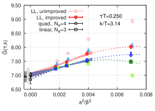
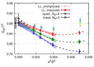
Figure 1: Left panel: Simultaneous continuum extrapolation at $\tau T=0.25$ of the local-local (LL), local-conserved (LC) and conserved-conserved (CC) tree-level improved correlators plotted with red circles, blue triangles and green squares, respectively. The unimproved correlator values are shown with fainter symbols. The coloured bands show the linear fit using the three finest lattice spacings and all discretizations, while the dashed lines illustrates the quadratic fit using all data points. The results of the linear (quadratic) extrapolations are shown as empty squares (circles). The fainter, shifted, grey symbols show the continuum values obtained using the unimproved correlators. The leftmost grey band represents our final continuum estimate, including its systematic error. Right panel: Simultaneous continuum extrapolation of the isovector charge-charge correlator required to compute the static susceptibility. The colour code is the same as on the left panel.

In order to estimate the systematic errors, we carried out extrapolations using the tree-level improved as well as the unimproved data. Further systematic variations included using two interpolation methods to interpolate to the same $\tau T$ points on all ensembles and varying the number of data points used in the fits. For the linear fits, only the three finest ensembles have been used and we investigated the robustness of the results by omitting one or two data points belonging to the coarsest two out of three ensembles. In the case of quadratic fits, we proceeded similarly, but we omitted one or two data points from the coarsest three out of four ensembles. When we left out more than one point, we always discarded them from the same discretization. Furthermore, we carried out extrapolations by using only one or two discretizations. These various changes in the analysis resulted in a total number of 104 fits. The $\chi^{2}$ values, the number of fit parameters and the number of data points have been used to calculate the Akaike Information Criterion (AIC) weight of each fit Akaike (1971); Borsanyi et al. (2021). Using these weights, we built a histogram and quoted the median as our final continuum result. The histogram is used in the later stages of the analysis.

We also perform the continuum limit of the static susceptibility, which requires including the $Z_{\mathrm{V}}$ renormalization constant when the local discretization of the current is used. To obtain the values of $Z_{\mathrm{V}}$ at the bare couplings of our ensembles, we utilized the parametrization of $Z_{\mathrm{V}}(g_{0}^{2})$ given in Ref. Della Morte et al. (2005). Then, adopting a similar procedure to determine the continuum limit of the static susceptibility as we used for the transverse correlator, we obtain $\chi_{\mathrm{s}}/T^{2}=\beta^{3}G_{00}(\beta/2,0)=0.882(11)_{\mathrm{stat}}(19)_{\mathrm{sys}}$, see the right panel of Fig. 1. Compared with our result of Ref. Cè et al. (2020), we quote a more conservative systematic error due to the continuum limit primarily due to the inclusion of quadratic fits in $a^{2}$ in this work. We have also investigated that the use of other determinations of the renormalization factor Dalla Brida et al. (2019) and the inclusion of the mass-dependent improvement, which lead to sub-leading differences compared to the systematic error from the continuum extrapolation.

In order to obtain $G_{\mathrm{T}}/T^{3}$ in the continuum, we multiplied the continuum limit of $G_{\mathrm{T}}/G_{00}$ by the continuum estimate of $G_{00}/T^{3}$. The transverse correlator divided by the charge-charge correlator is shown in the left panel of Fig. 2 for $k/T\approx 4.97$, and in units of temperature in the right panel. The statistical error on $G_{\mathrm{T}}/T^{3}$ is typically around $0.25-0.6\%$, while it is in the range $1.1-1.4\%$ for $G_{\mathrm{T}}/G_{00}$.

III.4 Continuum-extrapolated correlators vs. theory predictions

Having obtained the transverse-channel correlators in the continuum, we compare them to various theory predictions. In this comparison, we neglect the $O((m/T)^{2})$ quark-mass effects present in the lattice results, since $m/T\approx 0.05$ in our simulations.

We find that the LO correlator is about $5-20\%$ larger at Euclidean time separations $\tau T>0.4$ for momenta $k/T\gtrsim 3.85$; see Fig. 2. The deviation is smaller, around $\sim$ 5%, for smaller momenta. It reduces towards smaller time separations, and below a certain ($k$-dependent) $\tau T$ value, the LO correlator is smaller by about 5% than our continuum result. The NLO+LPM correlator, however, is only about $3-4\%$ larger than the lattice result for all momenta and for all time separations $0.17\lesssim\tau T\leq 0.5$ for which we could reliably determine the continuum limit. We conclude that the perturbative corrections to the LO correlator noticeably improve its agreement with our lattice correlator. The strongly coupled $\mathcal{N}=4$ SYM theory result also provides a relatively good description, even though that result concerns a different non-Abelian gauge theory and applies in the large-$N_{c}$ limit. The lower panels of Fig. 2 show the ratio of the perturbative and the SYM results to the lattice results.

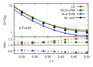
Figure 2: Left panel: Comparison of the $G_{\mathrm{T}}/G_{00}$ correlators. The bottom panels show the correlators normalized by the continuum correlator. The colour code is as in the top panel. The NLO+LPM result was obtained by using $\alpha_{\mathrm{s}}=0.25$. Right panel: Comparison of $G_{\mathrm{T}}/T^{3}$. We set $N_{\mathrm{c}}=3$ to obtain the SYM theory result.

A word on the multiplicative normalization of the theory predictions is in order. For the perturbative predictions, while no prescription is needed for $G(\tau,k)$, a choice must be make to obtain $\bar{G}(\tau,k)$. Here we have normalized both the LO and the NLO+LPM correlators by the $\mathrm{O}(g^{6}\ln g)$ susceptibility Vuorinen (2003). In Ref. Vuorinen (2003), the coefficient of one of the undetermined $\mathrm{O}(g^{6})$ term was estimated to be $C(N_{\mathrm{f}}=2)\approx-45$, which results in $\chi_{\mathrm{pert}}/T^{2}\approx 0.83$, the value which we used for Fig. 2. This value, however, is 6% lower than the continuum extrapolated value we obtained. Based on our lattice continuum result, $C(N_{\mathrm{f}}=2)\approx 33$ would result in a better agreement for $\chi_{\mathrm{s}}/T^{2}$. However, we note that the contributions from successive higher orders in the perturbative calculation of $\chi_{\mathrm{pert}}/T^{2}$ are similar in size, so the estimation for $C(N_{\mathrm{f}}=2)$ is to be treated with caution. As for the strongly coupled, large-$N_{c}$ $\mathcal{N}=4$ SYM correlator, we note that $\bar{G}(\tau,k)$ is a natural quantity to compare across different thermal systems; in particular, the dependence on the number of colours drops out. In order to compare the correlator $G(\tau,k)$ itself, a certain choice must be made for the susceptibility. We have chosen to set $\chi_{\mathrm{SYM}}/T^{2}=N_{\mathrm{c}}^{2}/8=9/8$.

IV Analysis of the transverse-channel spectral function

Given the transverse-channel Euclidean correlation function in the continuum limit, we proceed to analyze the corresponding spectral function via Eq. ​(6). Here, we present an analysis based directly on $G_{\mathrm{T}}/T^{3}$ in Secs. IV.1 and IV.2, since we found the correlator to be statistically particularly precise. In addition, we have seen that the NLO+LPM correlator is only a few percent off the lattice correlator, which encourages us to use that prediction as a baseline in Sec. ​IV.2. In contrast, since the primary continuum-extrapolated quantity was $\widebar{G}=G_{\mathrm{T}}/G_{00}$, Ref. ​Török et al. (2021) contains an analysis based on that ratio.

We start in Sec. ​IV.1 by using the Backus-Gilbert method in order to perform the comparison between lattice data and theory predictions in frequency space without introducing any model dependence. Sec. ​IV.2 then presents fits to the lattice data in order to determine the spectral function, with a particular focus on lightlike kinematics, $\omega=k$. For simplicity of notation, we omit the spatial momentum from the arguments in the following sections.

IV.1 Backus-Gilbert method: smeared spectral functions vs. theory predictions

The Backus-Gilbert method is a model-independent approach to overcome the spectral reconstruction problem Backus and Gilbert (1968). By using this method one can determine a local average of the spectral function around a given value of the frequency. In the present case it is also favourable to introduce a rescaling function, $f(\omega)$, which in particular removes the singularity at vanishing frequency of the kernel $K(\omega,\tau)$. Thus the new kernel is defined as

$$K_{f}(\omega,\tau)\equiv K(\omega,\tau)f(\omega),$$ (23)

with the rescaling function $f(\omega)$ being specified later, but satisfying $f(\omega)\propto\omega$ as $\omega\to 0$. The smeared, rescaled spectral function, $\hat{\rho}(\omega)/f(\omega)$, is defined in this case as

$$\frac{\hat{\rho}(\omega)}{f(\omega)}\equiv\int_{0}^{\infty}\mathrm{d}\omega^{\prime}\Delta(\omega,\omega^{\prime})\frac{\rho(\omega^{\prime})}{f(\omega^{\prime})},$$ (24)

where $\Delta(\omega,\omega^{\prime})$ is the so-called resolution function or averaging kernel, which is completely specified in terms of some coefficients, $g_{i}(\omega)$, and is given as

$$\Delta(\omega,\omega^{\prime})=\sum_{i}g_{i}(\omega)K_{f}(\omega^{\prime},\tau_{i}).$$ (25)

Inserting back $\Delta(\omega,\omega^{\prime})$ of Eq. (25) into Eq. (24), we find that the filtered spectral function is the linear combination of the Euclidean correlator data,

$$\hat{\rho}(\omega)=f(\omega)\sum_{i}g_{i}(\omega)G_{\rm{T}}(\tau_{i}).$$ (26)

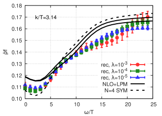
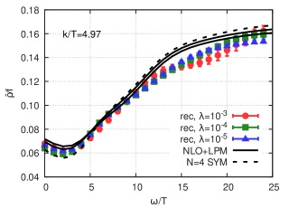
Figure 3: Comparison of filtered, rescaled, transverse channel spectral functions obtained using the continuum lattice data (with colours) and the perturbative spectral function (continuous, black) as well as the $\mathcal{N}=4$ SYM theory (dashed, black) for $k/T\approx 3.14$ and $k/T\approx 4.97$, left and right panel, respectively. The renormalization scale was set to $\mu=2\pi T$ or $\mu=3\pi T$ when using the NLO+LPM spectral function, which results in two curves. The renormalization scales $2\pi T$ and $3\pi T$ correspond to $\alpha_{\mathrm{s}}\simeq 0.31$ and $\alpha_{\mathrm{s}}\simeq 0.25$, respectively. Errors are only statistical.

The coefficients, $g_{i}(\omega)$, are determined in the Backus-Gilbert method by minimizing the second moment of the squared resolution function

$$A[g]\equiv\int_{0}^{\infty}\mathrm{d}\omega^{\prime}\,(\omega-\omega^{\prime})^{2}[\Delta(\omega,\omega^{\prime})]^{2}=\sum_{i,j}g_{i}(\omega)A_{ij}(\omega)g_{j}(\omega)$$ (27)

subject to the constraint

$$\int_{0}^{\infty}\mathrm{d}\omega^{\prime}\Delta(\omega,\omega^{\prime})=1.$$ (28)

This minimization ensures that the width of resolution function is as small as possible and that, at fixed $\omega$, $\Delta(\omega,\omega^{\prime})$ has unit area. The minimizing solution is given as

$$g_{i}(\omega)=\frac{A_{ij}^{-1}(\omega)R_{j}}{R_{k}A_{kl}^{-1}(\omega)R_{l}},$$ (29)

where

$$A_{ij}(\omega)=\int_{0}^{\infty}\mathrm{d}\omega^{\prime}K_{f}(\omega^{\prime},\tau_{i})K_{f}(\omega^{\prime},\tau_{j})(\omega-\omega^{\prime})^{2}\quad{\mathrm{and}}\quad R_{i}=\int_{0}^{\infty}\mathrm{d}\omega K_{f}(\omega,\tau_{i}).$$ (30)

The matrix ${\bf A}$ is ill-conditioned in practice, therefore an error functional is added to $A[g]$ which serves as a regulator. As a consequence, ${\bf A}$ has to be replaced by ${\bf A}^{\mathrm{reg}}$ in Eq. (29), where

$$A^{\mathrm{reg}}_{ij}(\omega)=\lambda A_{ij}(\omega)+(1-\lambda)\mathrm{Cov}_{ij}[G_{\mathrm{T}}],$$ (31)

and $0\leq\lambda\leq 1$ is the regularization parameter compromising between stability and resolution. The smaller the value of $\lambda$, the larger the regularization. In Eq. (31), $\mathrm{Cov}[G_{\mathrm{T}}]$ stands for the covariance matrix of the Euclidean correlator. We note that in our numerical implementation we worked in the units of temperature.

We emphasize again that from the filtered spectral function one cannot model-independently determine the value of $\rho(\omega)$ itself, but it could be useful to compare it to a similarly smoothened spectral function coming from other approaches. Once the $g_{i}(\omega)$ coefficients are determined via Eq. (29) by utilizing the covariance matrix of the data, the same resolution function can be used to build, for instance, the perturbative filtered spectral function. In Fig. 3, we compare the filtered spectral function obtained from the continuum $G_{\mathrm{T}}/T^{3}$ data to the filtered spectral function of the weak-coupling QCD regime as well as of the SYM theory, using the same resolution functions. The chosen rescaling function was

$$f(\omega)=\frac{\omega^{2}}{\tanh(\omega/(2T))}.$$ (32)

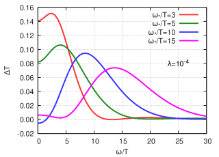
Figure 4: Resolution functions for $k/T\approx 3.14$, $\lambda=10^{-4}$ for different values of $\omega_{*}/T$.

As Fig. 3 shows, the filtered, rescaled spectral function obtained using the lattice data is somewhat below the perturbative one, especially for small momenta ($k/T\leq 3.14$). At small frequencies, below $\omega/T\sim 5$, the filtered spectral function is between the weak-coupling and the $\mathcal{N}=4$ SYM theory filtered spectral function. Using all nine data points for the correlator, we found that the condition number of ${\bf A}^{\rm{reg}}$ gets more or less tractable (smaller than $\sim 10^{7}$) when $\lambda$ is around $10^{-4}$ or smaller. The elements of ${\bf A}^{\rm{reg}}$ are still dominated in this case by the first term of Eq. (31), which are several orders of magnitude larger than the elements of the covariance matrix. When $\lambda\gtrsim 10^{-2}$, the condition number is above $5\times 10^{8}$ and $\hat{\rho}(\omega)$ tends to have unphysical wiggles. By omitting e.g. the first data point from the correlator, one can use larger values of $\lambda$, but one less coefficient. The results, nevertheless, do not change significantly.

The resolution functions, $\Delta(\omega,\omega^{\prime})$, are quite wide and they blur the fine details of the spectral function. They are almost identical for different momenta when fixing the value of $\lambda$. Their dependence on $\lambda$ is also very mild, but increases when going to a higher target $\omega$. Some examples can be seen in Fig. 4. We obtained similar results to those discussed above using the covariance matrix of $G_{\mathrm{T}}/G_{00}$ instead.

In summary, we have found that the filtered spectral functions derived from the continuum-extrapolated lattice data are close to the NLO+LPM spectral function filtered with the same resolution function, and that the agreement increases both with increasing $k$ and increasing $\omega$, up to $\omega\approx 10T$. Since beyond that point the resolution function extends to very high frequencies, residual cutoff effects in the lattice results could explain the differences observed with the NLO+LPM curves in that regime. At $k=\pi T$, the non-perturbative filtered spectral function undershoots the perturbative prediction, a point already noted in Ghiglieri et al. (2016) for the $2\rho_{\rm T}+\rho_{\rm L}$ channel relevant for the dilepton rate. Finally, we remark that the value of $[\hat{\rho}(\omega,k)/f(\omega)]_{\omega=k}$ found here is very much in the ballpark of the values obtained for $[\rho(\omega,k)/f(\omega)]_{\omega=k}$ with various fit ansätze for the spectral function (see Fig. 5 below), even though the resolution function is rather broad compared to $k$.

IV.2 The transverse-channel spectral function from fits to the Euclidean correlators

We now turn to turn to our direct attempt at determining the spectral function by fitting various ansätze to the transverse correlator. When specifying possible ansätze describing the transverse spectral function, we have taken into account the facts that it has to be odd in $\omega$, i.e. $\rho(-\omega)=-\rho(\omega)$, as well as positive for $\omega>0$, as shown in Ref. Cè et al. (2020). While the ansätze were chosen to be odd by construction, models were only excluded a posteriori if they violated positivity with a 68% confidence level.

The high-frequency behavior of the spectral function is dictated by perturbation theory, therefore we assumed the following form for the transverse spectral function

$$\rho(\omega)=\rho_{\mathrm{fit}}(\omega)(1-\Theta(\omega,\omega_{0},\Delta))+\rho_{\mathrm{pert}}(\omega)\Theta(\omega,\omega_{0},\Delta),$$ (33)

where $\rho_{\mathrm{pert}}$ is the NLO prediction for the transverse spectral function complemented with the LPM contribution near the light-cone,

$$\rho_{\mathrm{pert}}(\omega)=\rho_{\mathrm{NLO}}(\omega)+\rho_{\mathrm{LPM}}(\omega),$$ (34)

and

$$\Theta(\omega,\omega_{0},\Delta)=(1+\tanh[(\omega-\omega_{0})/\Delta])/2$$ (35)

is a smooth step function which controls how fast the perturbative contribution falls off around $\omega_{0}$ as $\omega$ is lowered. Using the decomposition of Eq. (33), we ensure that the perturbative part gives the dominant contribution above the chosen value of $\omega_{0}$, which we call the matching frequency. Moreover, the transition from the perturbative regime — assumed to be valid in the ultraviolet — can be realized in a smooth way without constraining any of the coefficients of the fit function.

For the fit function, $\rho_{\mathrm{fit}}(\omega)$, we considered the following two possible ansätze:

$$\frac{\rho_{\mathrm{fit,1}}(\omega)}{T^{2}}=\sum_{n=0}^{N_{\mathrm{p}}-1}A_{n}\left(\frac{\omega}{\omega_{0}}\right)^{1+2n},$$ (36)

where $N_{\mathrm{p}}$ denotes the number of fit parameters, and

$$\frac{\rho_{\mathrm{fit,2}}(\omega)}{T^{2}}=\,\begin{dcases}\,A_{0}\,\frac{\omega}{\omega_{0}}+A_{1}\left(\frac{\omega}{\omega_{0}}\right)^{3},&\text{if\,\,}\omega\leq k,\\ \,B_{0}\,\frac{\omega}{\omega_{0}}+B_{1}\left(\frac{\omega}{\omega_{0}}\right)^{3},&\text{if\,\,}\omega>k,\end{dcases}$$ (37)

where the free parameters have been chosen to be $A_{0},B_{0},B_{1}$, and $A_{1}$ has been fixed imposing continuity, $A_{1}=B_{1}+(B_{0}-A_{0})\omega_{0}^{2}/k^{2}$. In the latter case, we also carried out fits by setting $B_{0}$ to zero, i.e. having only two fit parameters. The spectral function of Eq. 33 including $\rho_{\mathrm{fit,1}}(\omega)$ or $\rho_{\mathrm{fit,2}}(\omega)$ is referred to in the following as the polynomial or the piecewise polynomial ansatz, respectively.

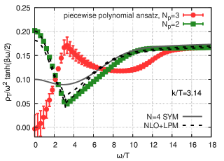
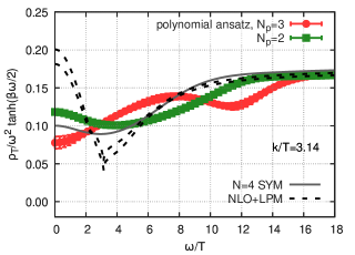
Figure 5: Left: Representative fit results using the piecewise polynomial ansatz with two ($N_{p}=2$) or three fit parameters ($N_{p}=3$) at $k/T=\pi$. For comparison, the transverse channel spectral function in the weak-coupling NLO+LPM theory, as well as in the strongly coupled SYM theory are also included. Right: Representative fit results using the polynomial ansatz.

These ansätze are motivated by their ability to describe the spectral function of the strongly coupled $\mathcal{N}=4$ SYM theory as well as that of the NLO+LPM resummed perturbation theory, to a satisfactory level. The functional form of Eq. (36) is more suitable for the spectral function obtained with the AdS/CFT approach in the $\mathcal{N}=4$ SYM theory, whereas the built-in non-differentiability at the light-cone in the piecewise polynomial ansatz of Eq. (37) is more apt at describing the cusp present in the NLO+LPM result. More details can be found about the expressivity of these ansätze in Appendix B, in which we present the outcome of mock data analyses and to which we return in the next subsection.

After inserting $\rho(\omega)$ from Eq. (33) into Eq. (6), we solved the correlated $\chi^{2}$-minimization problem to determine the unknown coefficients. We show some representative fit results with good $\chi^{2}$ values in Fig. 5 for the momentum $k=\pi T$. We explored many variations in the fit procedure and took into account the statistical and systematic error of the continuum-extrapolated Euclidean correlators. More details on this and the method of estimating systematic errors on the effective diffusion coefficient, $D_{\rm eff}(k)$, can be found in Appendix A. Our result for $D_{\rm eff}(k)$ extracted using the polynomial ansatz is displayed on the right panel of Fig. 6. The line within the band represents the median of the distribution of results obtained, while the width of the band indicates the position of the 16th and 84th percentile.

The piecewise polynomial fit ansatz turned out to yield a sizeable spread of results for the effective diffusion coefficient. This spread comes from the results for $D_{\mathrm{eff}}$ actually falling into two well separated intervals. Fit results with $N_{\mathrm{p}}=2$ tend to lead to results in the lower interval, while the results obtained with $N_{\mathrm{p}}=3$ populate both intervals. To illustrate the point, on the left panel of Fig. 6 we display the results for the effective diffusion coefficient $D_{\rm eff}(k)$ obtained with $N_{p}=2$ and $N_{p}=3$ separately as two coloured bands. This doubly-peaked distribution of results for $D_{\mathrm{eff}}$ is associated with the behaviour of the spectral function around lightlike kinematics. When using this ansatz to fit the correlator, we obtained spectral functions possessing either a minimum or a spike-like maximum at the light-cone frequency. Representative fit results are shown on the left panel of Fig. 5. Since neither the NLO+LPM weak-coupling nor the SYM spectral functions have a maximum at $\omega=k$, we also investigated the fit results obtained by excluding the fits satisfying

$$\frac{\mathrm{d}\rho}{\mathrm{d}\omega}\Big{|}_{\omega=k-\epsilon}-\frac{\mathrm{d}\rho}{\mathrm{d}\omega}\Big{|}_{\omega=k+\epsilon}>0$$ (38)

at least at one standard deviation. With this qualitative theoretical prejudice in place, the fit results are significantly more constraining. The $D_{\rm eff}$ values obtained this way are displayed on the right panel of Fig. 6, where they are denoted as “no-peak” solutions. Excluding fits possessing the feature Eq. (38) is also affirmed by the upper limit of the results obtained by analysing the spectral function in the $\mathrm{T}-\mathrm{L}$ channel Brandt et al. (2019); Cè et al. (2020). As can be seen by comparing the two panels of Fig. 6, a large portion of the solutions with a peak at lightlike kinematics can be excluded by our previous analysis of the $\mathrm{T}-\mathrm{L}$ channel. We note that the latter analysis has been carried out using the same ensembles that we employ in the present study. For comparison, Fig. 6 also displays the weak-coupling results (dashed lines) obtained directly for the photon rate in Ref. Arnold et al. (2001), as well as the strongly coupled SYM theory results (solid grey line).

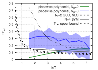
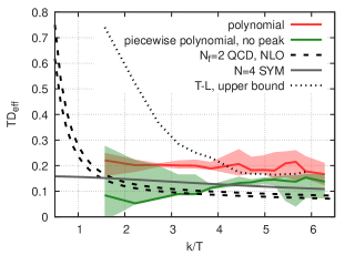
Figure 6: Results for the effective diffusion coefficient, $TD_{\mathrm{eff}}$, defined in Eq. (10). Left: Separate analyses of fit results obtained with $N_{\mathrm{p}}=2$ and $N_{\mathrm{p}}=3$ using the piecewise polynomial ansatz (Eq. (37)). Right: Imposing the constraint of Eq. (38) at one standard deviation to the fit results obtained with the piecewise polynomial ansatz. The results obtained by using the polynomial ansatz (Eq. (36)) are displayed in red. Analytical results from perturbative QCD Arnold et al. (2001) using $\alpha_{s}\simeq 0.25$ or 0.31 (dashed lines) and from the strongly coupled $\mathcal{N}=4$ SYM theory (grey line) Caron-Huot et al. (2006) are also included as well as an upper bound obtained from the analysis of the $\mathrm{T}-\mathrm{L}$ channel (dotted line) Cè et al. (2020). We use the value $\chi_{\mathrm{s}}/T^{2}=0.88(2)$ to obtain $TD_{\rm{eff}}$ from the lattice data, but the free susceptibility to obtain $TD_{\rm{eff}}$ from the $N_{\rm f}=2$ weak-coupling photon rate.

IV.3 Final result for the photon emissivity extracted from the fits

In order to arrive at our final estimate for the photon emissivity, we need to judge the reliability of our fit ansätze in extracting the quantity $D_{\rm eff}$. For this we return to the analysis of mock data, presented in detail in Appendix B. There, we found that the fit ansatz functions tend to overestimate the photon rate in the investigated models, irrespective of whether $G_{\mathrm{T}}/G_{00}$ or $G_{\mathrm{T}}/T^{3}$ is used. We therefore first derive an upper bound for $D_{\rm eff}$, and hence for the photon emissivity. By fitting a linear ansatz $a\times k/T+b$ to $TD_{\mathrm{eff}}$ obtained from the polynomial ansatz in the $k/T$ range $[\pi/2,2\pi]$ and then plugging the effective diffusion coefficient, $TD_{\mathrm{eff}}$, into the formula giving the thermal photon emission rate per unit volume, Eq. (2), we arrive at the following upper bound,

$$\frac{1}{T}\frac{\mathrm{d}\Gamma_{\gamma}(k)}{\mathrm{d}^{3}k}\leq\frac{\alpha_{\mathrm{em}}}{\pi^{2}}\,\frac{\chi_{\mathrm{s}}}{T^{2}}\,\frac{C_{\mathrm{em}}}{\mathrm{e}^{k/T}-1}\text{\small{$\times$}}\Big{(}0.22(1)-0.0062(25)\frac{k}{T}\Big{)}.$$ (39)

In Eq. (39), $C_{\mathrm{em}}$ denotes the charge factor equal to $2/3$ in the $N_{\mathrm{f}}=3$ theory. We recall that the static susceptibility has been determined in Sec. III.3, $\chi_{\mathrm{s}}/T^{2}=0.88(2)$ at $T\simeq 250$ MeV.

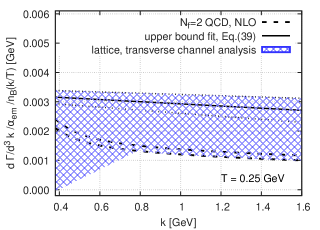
Figure 7: The photon rate per unit volume of the QGP at $T\simeq 250$ MeV (hatched band). The Bose factor $n_{\mathrm{B}}=1/(\mathrm{e}^{k/T}-1)$ has been divided out. The upper bound parametrization derived from the $D_{\rm eff}$ results of the polynomial ansatz is shown as a solid line. The full leading-order result Arnold et al. (2001) obtained by setting $\alpha_{\mathrm{s}}\simeq 0.25$ or 0.31 are shown for comparison. Including corrections from interactions with soft gluons, one can get a 20% increase at $\alpha_{\mathrm{s}}\simeq 0.3$ for the perturbative result Ghiglieri et al. (2013).

As far as a lower bound on $D_{\rm eff}$ is concerned, we distinguish two regimes, $k>\pi T$ and $k\leq\pi T$. In the former case, using the NLO+LPM correlator as input, the central value of the output for the effective diffusion constant is usually at least $50-80\%$ larger than the true value, and our error estimate typically does not cover the true value in the range $3.5\leq k/T\leq 5.5$ (see the right panel of Fig. 9). In the case of the $\mathcal{N}=4$ SYM theory mock data, the results from the two ansätze bracket the true result for intermediate and smaller momenta $k/T\lesssim 4.5$, but our ansätze overestimate $TD_{\mathrm{eff}}$ by $5-25\%$ at larger momenta. Therefore, for $k>\pi T$ we extend the lower bound down to the weak-coupling prediction in Fig. 6 (right panel), which we parametrize in Eq. (40).

For the mock data tests performed in the momentum range $k\leq\pi T$ on the other hand, the resulting error band always covers the true value for at least one of the two ansätze that we use. As the right panel of Fig. 6 shows, the lower bound is driven by the results of the piecewise polynomial ansatz, which decreases until reaching vanishing $D_{\rm eff}$ values at our smallest momentum. A parametrization of the lower bound can be given by a linear function in $k/T$ that connects zero at $k=\pi T/2$ and the NLO weak-coupling result at $k=\pi T$. Thus we parametrize our lower bound according to

$$\frac{1}{T}\frac{\mathrm{d}\Gamma_{\gamma}(k)}{\mathrm{d}^{3}k}\geq\frac{\alpha_{\mathrm{em}}}{\pi^{2}}\,\frac{\chi_{\mathrm{s}}}{T^{2}}\,\frac{C_{\mathrm{em}}}{\mathrm{e}^{k/T}-1}\text{\small{$\times$}}\left\{\begin{array}[]{ll}\big{(}-9.43+6.00\,\frac{k}{T}\big{)}\times 10^{-2},&\pi T/2\leq k\leq\pi T;\phantom{\Big{|}}\\ \big{(}4.86+14.33\,\frac{T}{k}\big{)}\times 10^{-2},&\pi T<k\leq 2\pi T.\end{array}\right.$$ (40)

From the observations made above, it is clear that this lower bound is influenced by the theory prejudice that the spectral function at lightlike kinematics does not ‘dive’ down to even smaller values than the weak-coupling results Arnold et al. (2001) predict for realistic values of $\alpha_{s}$; see Fig. 5.

We remark that the curves and bands displayed in Fig. 6 have a precise statistical meaning based on percentiles ($16^{\rm th}$, $50^{\rm th}$, $84^{\rm th}$) of the distribution of results obtained by applying a set of procedural variations. The band defined by the $k$-dependent bounds of Eqs. (39,40) summarizes the results, giving equal weight to both fit ansätze that we have used; it is displayed in Fig. 7.

V Conclusion

In this study, we have presented the first investigation of the transverse channel Euclidean correlator at finite momenta, using $N_{\mathrm{f}}=2$ $\mathrm{O}(a)$-improved dynamical Wilson fermions at around $T\simeq 250\,\mathrm{MeV}$ corresponding to $1.2T_{\mathrm{c}}$. We carried out a simultaneous continuum extrapolation using three discretizations of the correlators of the isovector vector currents. We used four ensembles with lattice spacings in the range $a\simeq 0.033\,$–$\,0.066$ fm. We compared the filtered spectral functions obtained from the continuum extrapolated transverse correlator via the Backus-Gilbert method to the spectral function of perturbation theory at next-to-leading order and the one obtained in the strongly coupled $\mathcal{N}=4$ supersymmetric Yang-Mills theory. The small-frequency lattice results lie between the filtered spectral functions obtained in these two theories. In order to determine the thermal photon emission rate, we fitted the correlators using polynomial and piecewise polynomial fit ansätze for the underlying spectral function. We validated the expressivity of these ansätze by performing mock tests using the spectral functions obtained in perturbation theory as well as in the $\mathcal{N}=4$ super Yang-Mills theory. We compared our results for the effective diffusion coefficient to the results obtained in these theories as shown in Fig. 6, and also to the results obtained by analysing the difference of the transverse and the longitudinal channels, presented earlier in Ref. Cè et al. (2020). The ranges obtained are compatible with the weak-coupling as well as with the AdS/CFT results. Our final result for the photon emissivity is displayed in Fig. 7 as a hatched band, for which we provide a parametrization in Eqs. (39,40). For momenta below 1 GeV, the upper edge of the band is more constraining than the estimate derived from the analysis of the difference of the transverse and longitudinal channels. We obtain our strongest constraint on the photon emissivity around $k=\pi T\simeq 0.8\,$GeV,

$$\frac{\mathrm{d}\Gamma_{\gamma}}{\mathrm{d}^{3}k}=\frac{\alpha_{\rm em}}{e^{k/T}-1}\,(2.2\pm 0.8)\times 10^{-3}\,{\rm GeV}.$$ (41)

In the future, we plan to (linearly) combine the present analysis with our previous one Cè et al. (2020) to provide estimates of the dilepton rate at invariant masses $M_{\ell^{+}\ell^{-}}^{2}=\omega^{2}-k^{2}>0$. We are also investigating a qualitatively different approach to the photon rate by computing zero-virtuality correlators on the lattice Meyer (2018); Cè et al. (2021). Whilst numerically challenging, this approach allows one to avoid confronting the inverse problem.

Appendix A Technical aspects of the fits for the spectral function

In this appendix, we provide some details on the procedure we followed in Sec. IV.2 to obtain spectral functions via fits to the Euclidean correlators. After inserting $\rho(\omega)$ from Eq. (33) into Eq. (6), we solved the correlated $\chi^{2}$-minimization problem to determine the unknown coefficients. When doing so, we regularized the covariance matrix by multiplying the off-diagonal elements by 0.95. To estimate the statistical error, the minimization problem has been solved for every jackknife sample of the continuum correlator by using the covariance matrix obtained from the full data. To quantify the systematic uncertainty of the reconstruction coming from the systematic uncertainty of the continuum limit correlator values, we used the continuum extrapolation fit results for the 16th, 50th and 84th percentile of the AIC-weighted histogram obtained for each $\tau T$ value. However, we did not take into account all possible combinations of these histogram representatives, but chose random subsets containing 20 – 100 combinations for each momentum.

In order to estimate the systematic error from making parameter choices for the perturbative results or changing various parameters when fitting, we performed several fits using a set of plausible variants. Regarding the perturbative input for our analysis, the NLO+LPM result depends on the coupling constant. Using the four-loop formulae of Ref. Deur et al. (2016), we determined the coupling constant by setting the renormalization scale either to $\mu=2\pi T$ or to $\mu=3\pi T$. The coupling constants corresponding to these choices are $\alpha_{\mathrm{s}}\simeq 0.31$ and $\alpha_{\mathrm{s}}\simeq 0.25$, respectively. We took $\Lambda_{\overline{\rm MS}}^{(N_{\mathrm{f}}=2)}$ from the FLAG report Aoki et al. (2020).

source of systematic error	variations
#(correlator data pts)	9, 8, 7, 6
#(fit parameters)	2, 3
soft: $\Delta/T$	1.6, 2.0, 2.4
$\omega_{0}/T$	10, 12
ren. scale	$(2,3)\times\pi T$

Table 1: Summary of the systematic variations we employed in the fit approach. Using nine (six) data points correspond to fitting from $\tau T\approx$ 0.167 (0.292).

We applied two values for the matching frequency, $\omega_{0}=10T$ and $\omega_{0}=12T$, which correspond to 2.5 GeV and 3 GeV, respectively. For the parameter $\Delta$ in $\Theta(\omega,\omega_{0},\Delta)$, which governs the falloff of the NLO+LPM contribution towards the infrared, we set $\Delta=2T$, allowing also for a 20% variation. As a further systematic variation, we adjusted the fit ranges in $\tau T$ to include more or fewer data points in the fits. The variations we applied for the systematic error estimation are summarized in Table 1. Due to these variations, we collected 750–2000 fits with $p$-values larger than 0.05 for each momentum when using the polynomial ansatz, and around 15–30% of these fits had $p$-values larger than 0.5. When using the piecewise polynomial ansatz, we also obtained a lot of fits with good $\chi^{2}$ (and $p$-values). The fraction of the number of fits with $p$-values greater than 0.5 was around 15–30% in that case as well. We built an AIC-weighted histogram from the fit results that we used to estimate the systematic errors Akaike (1971); Borsanyi et al. (2021).

Appendix B Mock analyses

We performed mock analyses to see whether the fit ansätze are expressive enough to reproduce the transverse channel spectral function as well as to investigate the reliability of the Backus-Gilbert method. For these tests, we used two models:

• the NLO weak-coupling spectral function complemented with the LPM contribution near the light-cone and

• the spectral function of the strongly coupled $\mathcal{N}=4$ super Yang-Mills (SYM) theory.

We generated mock correlators using an appropriately rescaled covariance matrix of the lattice covariance matrix, which was obtained with the help of the continuum extrapolated correlator and the jackknife samples.

The procedure we followed consists of the following steps:

1. calculation of the ratio, $r(\tau)$, of the model and the continuum lattice correlator, $r(\tau):=G_{\mathrm{model}}(\tau)/G(\tau)$;

2. rescaling the covariance matrix of $G$ in the continuum: $\mathrm{Cov}_{\mathrm{resc},\,\tau\tau^{\prime}}:=\mathrm{Cov}_{\tau\tau^{\prime}}\,r(\tau)r(\tau^{\prime})$;

3. generating multivariate Gaussian variables, $G_{\mathrm{mock}}(\tau)$, using the rescaled covariance matrix, $\mathrm{Cov}_{\mathrm{resc}}$, as well as $G_{\mathrm{model}}(\tau)$;

4. determination of the ratio $\bar{r}(\tau)$ of the mock correlator, $G_{\mathrm{mock}}(\tau)$, and the lattice continuum correlator;

5. rescaling all jackknife samples using $\bar{r}(\tau)$ and calculating the covariance matrix of the mock correlator ($\mathrm{Cov}_{\mathrm{mock}}$) using these rescaled values.

We used then $G_{\mathrm{mock}}(\tau)$ and $\mathrm{Cov}_{\mathrm{mock}}$ in the fit analysis. The mock jackknife samples have been used to estimate the statistical error in the mock analysis. The relative errors of the mock correlator are roughly the same as the relative errors of the continuum extrapolated correlator due to the rescaling. We found that applying only step 1 and step 2 of the procedure above, complemented with a simple rescaling of the jackknife samples with $r(\tau)$ results in the overestimation of errors.

In addition to using the same relative errors as the continuum lattice data, we also investigated the effect of reducing the errors on the mock correlator and therefore included slight modifications to the above procedure. Introducing the error reduction factor, $s>1$, we used $r(\tau)/s$ in step 2, and instead of a rescaling, we determined the $j$th jackknife mock correlator value as $\bar{G}_{\mathrm{mock}}^{(j)}(\tau)=\bar{G}_{\mathrm{mock}}(\tau)+\left(r(\tau)\bar{G}^{(j)}(\tau)-\bar{G}_{\mathrm{mock}}(\tau)\right)/s$ in step 5.

Since we extrapolated $\widebar{G}=G_{\mathrm{T}}/G_{00}$ to the continuum (see Sec. III.3), we also carried out the mock analysis using this observable. When doing so, $G$, $G_{\mathrm{mock}}$ and $G_{\mathrm{model}}$ should be replaced by $\widebar{G}$, $\widebar{G}_{\mathrm{mock}}$ and $\widebar{G}_{\mathrm{model}}$, respectively, in the above procedure, and we refer to this ratio of the chosen model when we have e.g. $\widebar{G}_{\mathrm{model}}$. Since the covariance matrices are quite different for $G_{\mathrm{T}}/T^{3}$ and for $G_{\mathrm{T}}/G_{00}$, the mock analyses starting from the former or the latter result in different outcomes.

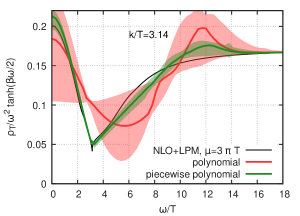
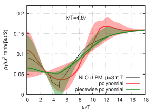
Figure 8: Reconstructed spectral functions using the NLO+LPM weak-coupling $G_{\mathrm{T}}/G_{00}$ mock correlator as an input.

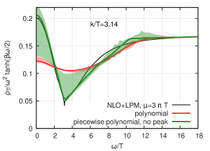
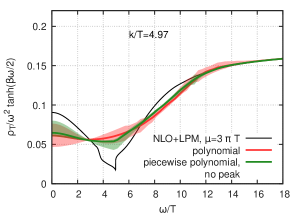
Figure 9: Reconstructed spectral functions using the NLO+LPM weak-coupling $G_{\mathrm{T}}/T^{3}$ mock correlator as an input.

When using the NLO weak-coupling mock correlator as an input for the reconstruction via fitting, we applied some variations in the fit setup, similar to the case of the analysis of the continuum extrapolated correlator (Sec. IV.2). These include using either two or three fit parameters in the fit ansätze, changing the number of the correlator data points utilized in the fit, and changing the features ($\omega_{0}/T,\Delta/T$) of the matching to the UV behavior. Since when producing the mock correlator, we generated multivariate Gaussian variables randomly, to eliminate a possible effect coming from the random input, we used six different mock correlators generated with the procedure discussed above. The systematic error have been estimated using the AIC-weighted histogram of the various fit results, and we used the mock jackknife samples to estimate the statistical error of the mock analyses. The same fit ansatz functions — Eq. (36) and Eq. (37) — have been applied as in the main analysis.

We found that both fit ansätze perform reasonably well in the weak-coupling case when using the $G_{\mathrm{T}}/G_{00}$ data, see Fig. 8. Namely, above $k/T\approx\pi$, both ansätze reproduce the input spectral functions within errors in a wide range of $\omega/T$ values also at small and large frequencies. The errors, however, are typically larger in this case for the polynomial ansatz ($\sim$ 10 – 50%, but even could be 100% at certain frequencies), than when using the $G_{\mathrm{T}}/T^{3}$ data (errors < 2 – 8%). At $\omega=k$, however, the polynomial ansatz gives a much larger value of $\rho$, i.e. a larger photon rate, using either $G_{\mathrm{T}}/G_{00}$ or $G_{\mathrm{T}}/T^{3}$. The piecewise polynomial ansatz could reproduce the features of the NLO+LPM mock data better, because it is capable of producing a sharper dip at the light-cone. With the help this ansatz, we get smaller photon rates at small momenta (below $k/T\approx\pi$), and larger photon rates at larger momenta, but in this latter case with errors spreading towards smaller values, typically covering the true spectral function at the light-cone. Using the $G_{\mathrm{T}}/T^{3}$ mock data, this ansatz — similarly to the polynomial ansatz — also returns a larger photon rate at all momenta, see e.g. Fig. 9. In this case, the error covers the bottom of the dip only at and below $k/T=\pi$.

The reproduction of the mock spectral function can be improved by a certain amount by reducing the errors on the input mock correlators. As Fig. 12 shows, accomodating an error reduction factor of $s=10$, the piecewise polynomial ansatz could mimic the dip at $\omega=k$ at a more satisfactory level. For comparison, see the right panel of Fig. 8 and also that of Fig. 9. This observation shows that this particular ansatz having only a few parameters has satisfactory expressiveness of reproducing a model spectral function relevant to the physics discussed in this paper. Conversely, it also indicates that the fact that we obtained less faithful spectral function outcomes when not reducing the error is mainly due to the covariance matrix and not due to a wrong choice of ansätze.

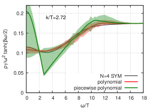
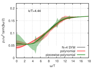
Figure 10: Reconstructed spectral functions using the strongly coupled $\mathcal{N}=4$ SYM theory mock correlator, $G_{\mathrm{T}}/G_{00}$, as an input.

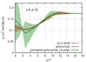
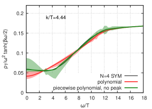
Figure 11: Reconstructed spectral functions using the strongly coupled $\mathcal{N}=4$ SYM theory mock correlator, $G_{\mathrm{T}}/T^{3}$, as an input.

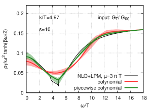
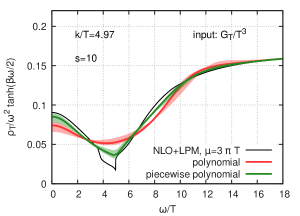
Figure 12: Reconstructed spectral functions using the NLO+LPM correlator $G_{\mathrm{T}}/G_{00}$ (left panel), or $G_{\mathrm{T}}/T^{3}$ (right panel) as an input. The covariance matrix elements have been decreased by a factor of $s^{2}=100$. Having so small errors, the piecewise polynomial ansatz could better approximate the dip.

Performing mock tests using the strongly coupled $\mathcal{N}=4$ SYM theory transverse correlators, the polynomial ansatz adequately reproduces the spectral function even for small momenta with errors less than around 5 – 10% for frequencies around and above $\omega=k$, see Fig. 10 and Fig. 11. As one goes for higher momenta, the reproduction gets a bit worse, but usually with errors included, one reaches the true values of the input spectral function. The photon rates given by this ansatz are always higher than the true photon rate, either using the mock $G_{\mathrm{T}}/G_{00}$ or the $G_{\mathrm{T}}/T^{3}$ data, see Fig. 10 and Fig. 11, respectively. The deviation increases from about 2% corresponding to smaller momenta up to 25% for high momenta.

For this model, the piecewise polynomial ansatz could also give reasonably good results for high momenta, where it almost coincides with the polynomial ansatz results. For momenta, $k/T<4.44$, it always gives a smaller photon rate, not depending on using $G_{\mathrm{T}}/G_{00}$ or $G_{\mathrm{T}}/T^{3}$, but in the latter case the central value is much closer to the true value.

The mock data also served as a numerical crosscheck for the Backus-Gilbert method, both using $G_{\mathrm{T}}/G_{00}$ as well as $G_{\mathrm{T}}/T^{3}$. As Fig. 13 shows, the Backus-Gilbert method is capable of reproducing the smeared, rescaled spectral function up to around $\omega/T\sim 16$.

Figure 13: Reconstructed, filtered spectral functions using the $\mathcal{N}=4$ SYM mock correlator, $\bar{G}^{(\mathrm{mock})}=G^{(\mathrm{mock})}_{\mathrm{T}}/G^{(\mathrm{mock})}_{00}$, as an input. The results obtained with the help of the 6 randomized mock correlators are shown in orange without including the statistical errors. These errors are comparable to the errors of the reconstructed $\hat{\rho}$ using the exact model data.

References

- Feinberg (1976) E. L. Feinberg, Nuovo Cim. A 34, 391 (1976).
- Shuryak (1978) E. V. Shuryak, Phys. Lett. B 78, 150 (1978).
- Ferbel and Molzon (1984) T. Ferbel and W. R. Molzon, Rev. Mod. Phys. 56, 181 (1984).
- Cassing and Bratkovskaya (1999) W. Cassing and E. L. Bratkovskaya, Phys. Rept. 308, 65 (1999).
- David (2020) G. David, Rept. Prog. Phys. 83, 046301 (2020), eprint 1907.08893.
- Adare et al. (2015) A. Adare et al. (PHENIX), Phys. Rev. C 91, 064904 (2015), eprint 1405.3940.
- Adamczyk et al. (2017) L. Adamczyk et al. (STAR), Phys. Lett. B 770, 451 (2017), eprint 1607.01447.
- Adam et al. (2016) J. Adam et al. (ALICE), Phys. Lett. B 754, 235 (2016), eprint 1509.07324.
- Paquet et al. (2016) J.-F. Paquet, C. Shen, G. S. Denicol, M. Luzum, B. Schenke, S. Jeon, and C. Gale, Phys. Rev. C 93, 044906 (2016), eprint 1509.06738.
- Gale et al. (2021) C. Gale, J.-F. Paquet, B. Schenke, and C. Shen (2021), eprint 2106.11216.
- Arnold et al. (2001) P. B. Arnold, G. D. Moore, and L. G. Yaffe, JHEP 12, 009 (2001), eprint hep-ph/0111107.
- Ghiglieri et al. (2013) J. Ghiglieri, J. Hong, A. Kurkela, E. Lu, G. D. Moore, et al., JHEP 1305, 010 (2013), eprint 1302.5970.
- Aarts and Martinez Resco (2002) G. Aarts and J. M. Martinez Resco, JHEP 04, 053 (2002), eprint hep-ph/0203177.
- Teaney (2006) D. Teaney, Phys. Rev. D 74, 045025 (2006), eprint hep-ph/0602044.
- Meyer (2011) H. B. Meyer, Eur. Phys. J. A 47, 86 (2011), eprint 1104.3708.
- Borsányi et al. (2018) S. Borsányi, Z. Fodor, M. Giordano, S. D. Katz, A. Pasztor, C. Ratti, A. Schäfer, K. K. Szabo, and B. C. Tóth, Phys. Rev. D 98, 014512 (2018), eprint 1802.07718.
- Ding et al. (2011) H.-T. Ding, A. Francis, O. Kaczmarek, F. Karsch, E. Laermann, et al., Phys. Rev. D 83, 034504 (2011), eprint 1012.4963.
- Brandt et al. (2013) B. B. Brandt, A. Francis, H. B. Meyer, and H. Wittig, JHEP 03, 100 (2013), eprint 1212.4200.
- Amato et al. (2013) A. Amato, G. Aarts, C. Allton, P. Giudice, S. Hands, et al., Phys. Rev. Lett. 111, 172001 (2013), eprint 1307.6763.
- Aarts et al. (2015) G. Aarts, C. Allton, A. Amato, P. Giudice, S. Hands, and J.-I. Skullerud, JHEP 02, 186 (2015), eprint 1412.6411.
- Brandt et al. (2016a) B. B. Brandt, A. Francis, B. Jaeger, and H. B. Meyer, Phys. Rev. D 93, 054510 (2016a), eprint 1512.07249.
- Ding et al. (2016) H.-T. Ding, O. Kaczmarek, and F. Meyer, Phys. Rev. D 94, 034504 (2016), eprint 1604.06712.
- Ghiglieri et al. (2016) J. Ghiglieri, O. Kaczmarek, M. Laine, and F. Meyer, Phys. Rev. D 94, 016005 (2016), eprint 1604.07544.
- Cè et al. (2020) M. Cè, T. Harris, H. B. Meyer, A. Steinberg, and A. Toniato, Phys. Rev. D 102, 091501 (2020), eprint 2001.03368.
- Backus and Gilbert (1968) G. Backus and F. Gilbert, Geophys. J. Int. 16, 169 (1968).
- Backus and Gilbert (1970) G. Backus and F. Gilbert, Philos. T. R. Soc. A 266, 123 (1970).
- McLerran and Toimela (1985) L. D. McLerran and T. Toimela, Phys. Rev. D 31, 545 (1985).
- Brandt et al. (2018) B. B. Brandt, A. Francis, T. Harris, H. B. Meyer, and A. Steinberg, EPJ Web Conf. 175, 07044 (2018), eprint 1710.07050.
- Brandt et al. (2019) B. B. Brandt, M. Cè, A. Francis, T. Harris, H. B. Meyer, A. Steinberg, and A. Toniato, PoS LATTICE2019, 225 (2019), eprint 1912.00292.
- Hong and Teaney (2010) J. Hong and D. Teaney, Phys. Rev. C 82, 044908 (2010), eprint 1003.0699.
- Baier et al. (1988) R. Baier, B. Pire, and D. Schiff, Phys. Rev. D 38, 2814 (1988).
- Aarts and Martinez Resco (2005) G. Aarts and J. M. Martinez Resco, Nucl. Phys. B 726, 93 (2005), eprint hep-lat/0507004.
- Laine (2013) M. Laine, JHEP 11, 120 (2013), eprint 1310.0164.
- Ghisoiu and Laine (2014) I. Ghisoiu and M. Laine, JHEP 10, 083 (2014), eprint 1407.7955.
- Jackson (2019) G. Jackson, Phys. Rev. D 100, 116019 (2019), eprint 1910.07552.
- Jackson and Laine (2019) G. Jackson and M. Laine, JHEP 11, 144 (2019), eprint 1910.09567.
- Aurenche et al. (2000) P. Aurenche, F. Gelis, and H. Zaraket, Phys. Rev. D 62, 096012 (2000), eprint hep-ph/0003326.
- Aurenche et al. (2002) P. Aurenche, F. Gelis, G. D. Moore, and H. Zaraket, JHEP 12, 006 (2002), eprint hep-ph/0211036.
- Carrington et al. (2008) M. E. Carrington, A. Gynther, and P. Aurenche, Phys. Rev. D 77, 045035 (2008), eprint 0711.3943.
- Caron-Huot et al. (2006) S. Caron-Huot, P. Kovtun, G. D. Moore, A. Starinets, and L. G. Yaffe, JHEP 12, 015 (2006), eprint hep-th/0607237.
- Fritzsch et al. (2012) P. Fritzsch, F. Knechtli, B. Leder, M. Marinkovic, S. Schaefer, R. Sommer, and F. Virotta, Nucl. Phys. B 865, 397 (2012), eprint 1205.5380.
- Brandt et al. (2016b) B. B. Brandt, A. Francis, H. B. Meyer, O. Philipsen, D. Robaina, and H. Wittig, JHEP 12, 158 (2016b), eprint 1608.06882.
- Engel et al. (2015) G. P. Engel, L. Giusti, S. Lottini, and R. Sommer, Phys. Rev. Lett. 114, 112001 (2015), eprint 1406.4987.
- Steinberg (2021) A. Steinberg, Ph.D. thesis, Mainz U. (2021).
- Akima (1970) H. Akima, J. ACM 17, 589–602 (1970).
- Steffen (1990) M. Steffen, Astronomy and Astrophysics 239, 443 (1990).
- Galassi et al. (2019) M. Galassi et al. (2019), URL https://www.gnu.org/software/gsl/.
- Akaike (1971) H. Akaike, in Petrov, B. N.; Csáki, F. (eds.), 2nd International Symposium on Information Theory, Tsahkadsor, Armenia, USSR, September 2-8 p. pp. 267–281. (1971).
- Borsanyi et al. (2021) S. Borsanyi et al., Nature 593, 51 (2021), eprint 2002.12347.
- Della Morte et al. (2005) M. Della Morte, R. Hoffmann, F. Knechtli, R. Sommer, and U. Wolff, JHEP 07, 007 (2005), eprint hep-lat/0505026.
- Dalla Brida et al. (2019) M. Dalla Brida, T. Korzec, S. Sint, and P. Vilaseca, Eur. Phys. J. C 79, 23 (2019), eprint 1808.09236.
- Vuorinen (2003) A. Vuorinen, Phys. Rev. D 67, 074032 (2003), eprint hep-ph/0212283.
- Török et al. (2021) C. Török, M. Cè, T. Harris, A. Krasniqi, H. B. Meyer, and A. Toniato, PoS LATTICE2021, 172 (2021), eprint 2112.00563.
- Meyer (2018) H. B. Meyer, Eur. Phys. J. A 54, 192 (2018), eprint 1807.00781.
- Cè et al. (2021) M. Cè, T. Harris, H. B. Meyer, A. Toniato, and C. Török (2021), eprint 2112.00450.
- Fousse et al. (2007) L. Fousse, G. Hanrot, V. Lefèvre, P. Pélissier, and P. Zimmermann, ACM Trans. Math. Softw. 33, 13–es (2007).
- Granlund and the GMP development team (2020) T. Granlund and the GMP development team (2020), URL https://gmplib.org/.
- Deur et al. (2016) A. Deur, S. J. Brodsky, and G. F. de Teramond, Nucl. Phys. 90, 1 (2016), eprint 1604.08082.
- Aoki et al. (2020) S. Aoki et al. (Flavour Lattice Averaging Group), Eur. Phys. J. C 80, 113 (2020), eprint 1902.08191.