Power Scaling Law for Optical IRSs and Comparison with Optical Relays

Abstract

The line-of-sight (LOS) requirement of free-space optical (FSO) systems can be relaxed by employing optical relays and optical intelligent reflecting surfaces (IRSs). Unlike radio frequency (RF) IRSs, which typically exhibit a quadratic power scaling law, the power reflected from FSO IRSs and collected at the receiver lens may scale quadratically or linearly with the IRS size or may even saturate at a constant value. We analyze the power scaling law for optical IRSs and unveil its dependence on the wavelength, transmitter (Tx)-to-IRS and IRS-to-receiver (Rx) distances, beam waist, and lens size. We compare optical IRSs in different power scaling regimes with optical relays in terms of the outage probability, diversity and coding gains, and optimal placement. Our results show that, at the expense of a higher hardware complexity, relay-assisted FSO links yield a better outage performance at high signal-to-noise-ratios (SNRs), but optical IRSs can achieve a higher performance at low SNRs. Moreover, while it is optimal to place relays equidistant from Tx and Rx, the optimal location of IRSs depends on the power scaling regime they operate in.

I Introduction

Due to their directional narrow laser beams and easy-to-install transceivers, free space optical (FSO) systems are promising candidates for high data rate applications, such as wireless front- and back-hauling, in next generation wireless communication networks and beyond [1]. FSO systems require a line-of-sight (LOS) connection between transmitter (Tx) and receiver (Rx) which can be relaxed by using optical relays [2] or optical intelligent reflecting surfaces (IRSs) [3, 4, 5]. Optical relays process the incident signal and forward an amplified signal to the receiver. For high data rate FSO systems, relays may require high-speed decoding and encoding hardware and/or analog gain units, additional synchronization, and clock recovery [6]. On the other hand, optical IRSs are planar structures comprised of passive subwavelength elements, known as unit cells, which can manipulate the properties of an incident wave such as its phase and polarization [7, 8]. In particular, to redirect an incident beam in a desired direction, the IRS can apply a phase shift to the incident wave and adjust the accumulated phase of the reflected wave [9].

For radio frequency (RF) IRSs, the received power typically scales quadratically with the IRS area, $\Sigma_{\text{irs}}$, [10, 11]. However, for optical IRSs, depending on the receiver lens size, the location of Tx and Rx with respect to (w.r.t.) the IRS, and the beam waist, the received power may scale quadratically ($\mathcal{O}(\Sigma_{\text{irs}}^{2})$) or linearly ($\mathcal{O}(\Sigma_{\text{irs}})$) with the IRS size or it may even saturate to a constant value ($\mathcal{O}(1)$) [12]. In this paper, we analyze the power scaling law for optical IRSs in detail in terms of the system parameters.

Furthermore, we compare the performance of relay- and IRS-assisted FSO systems. Such comparisons were made for RF IRSs with decode-and-forward (DF) and amplify-and-forward (AF) relays in [13] and [14], respectively. However, RF links are fundamentally different from FSO links in the following aspects: 1) While spherical/planar RF waves lead to a uniform power distribution across the IRS, FSO systems employ Gaussian laser beams, which have a curved wavefront and a non-uniform power distribution [9]; 2) Unlike in RF links, the variance of the fading affecting FSO links is distance-dependent [2]; 3) To reduce hardware complexity, mostly half-duplex relays are employed in RF systems, whereas FSO relays are typically full-duplex [15]; 4) The electrical size of the IRS (IRS length divided by the wavelength) at optical frequencies is much larger than at RF.

In this paper, we consider relay- and IRS-assisted FSO systems and our contributions are summarized as follows: First, we analyze the power scaling law for different IRS sizes, and then, we compare the performance of IRS- and relay-assisted FSO systems in terms of outage probability. Our results show that, at the expense of higher hardware complexity, relay-assisted FSO links yield a higher diversity gain as the variance of the corresponding distance-dependent fading is smaller compared to that of IRS-assisted FSO links. Moreover, the coding gain in IRS-based FSO links may increase with the IRS size depending on the power scaling regime the IRS operates in. We also analyze the optimal positions of the FSO relays and IRSs for maximization of the end-to-end performance. We show that while relays are optimally positioned equidistant from Tx and Rx [16, 15], the optimal position of the IRS depends on the power scaling regime. In particular, the optimal placement of the IRS is close to Tx or Rx, close to Tx, and equidistant from Tx and Rx if the IRS operates in the quadratic, linear, and saturation power scaling regime, respectively.

II System and Channel Models

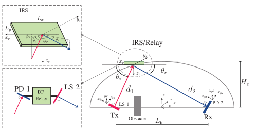
Figure 1: IRS- and relay-based FSO systems with end-to-end distance $d_{3}=d_{1}+d_{2}$ and Tx-to-Rx distance $L_{\text{tr}}$.

We consider two FSO systems, where Tx and Rx are connected via an IRS and a relay, respectively. Tx and Rx are located on the $x$-axis with distance $L_{\text{tr}}\over 2$ from the origin of the $xyz$-coordinate system, see Fig. 1. Moreover, the centers of the IRS and the relay are located at the origin of the $x_{r}y_{r}z_{r}$-coordinate system, where the $x_{r}y_{r}$-plane is parallel to the $xy$-plane and the $z_{r}$-axis points in the opposite direction of the $z$-axis, see Fig. 1. The Tx is equipped with laser source (LS) 1 emitting a Gaussian laser beam. The beam axis intersects with the $x_{r}y_{r}$-plane at distance $d_{1}$ and in direction $\mathbf{\Psi}_{i}=\left(\theta_{i},\phi_{i}\right)$, where $\theta_{i}$ is the angle between the $x_{r}y_{r}$-plane and the beam axis, and $\phi_{i}$ is the angle between the projection of the beam axis on the $x_{r}y_{r}$-plane and the $x_{r}$-axis. Moreover, the Rx is equipped with photo-detector (PD) 2 and a circular lens of radius $a$. The lens of the Rx is located at distance $d_{2}$ from the origin of the $x_{r}y_{r}z_{r}$-coordinate system. The normal vector of the lens plane points in direction $\mathbf{\Psi}_{r}=\left(\theta_{r},\phi_{r}\right)$, where $\theta_{r}$ is the angle between the $x_{r}y_{r}$-plane and the normal vector, and $\phi_{r}$ is the angle between the projection of the normal vector on the $x_{r}y_{r}$-plane and the $x_{r}$-axis. We assume that the Rx lens plane is always perpendicular to the axis of the received beam. In the following, we describe the relay- and IRS-assisted FSO systems more in detail.

II-A Relay-Assisted FSO System Model

We assume the Tx is connected to the Rx via a full-duplex DF relay where the relay receives the transmitted symbols via PD 1, re-encodes the signal, and transmit it via LS 2 to PD 2 at the Rx. PD 1 is equipped with a circular lens of radius $a$ which is always perpendicular to the axis of the received beam. Assuming an intensity modulation and direct detection (IM/DD) system, the received signal intensity at the relay, $y_{1}$, is given by

$$y_{1} =\sqrt{P_{1}}h_{1}s_{1}+n_{1},$$ (1)

where $s_{1}$ is the symbol transmitted by LS 1 with $\mathbb{E}\{|s_{1}|^{2}\}=1$, $P_{1}$ is the transmit power of LS 1, $h_{1}\in\mathcal{R}^{+}$ denotes the gain of the Tx-to-relay link, and $n_{1}\sim\mathcal{N}\left(0,\sigma_{n}^{2}\right)$ is the additive white Gaussian noise (AWGN) at PD 1 with zero mean and variance $\sigma_{n}^{2}$. Here, $\mathbb{E}\{\cdot\}$ denotes expectation. Then, the received signal intensity at PD 2, $y_{2}$, is given by

$$y_{2} =\sqrt{P_{2}}h_{2}s_{2}+n_{2},$$ (2)

where $s_{2}$ is the signal transmitted by the relay with $\mathbb{E}\{|s_{2}|^{2}\}=1$, $h_{2}\in\mathcal{R}^{+}$ denotes the FSO channel gain of the relay-to-Rx link, $P_{2}$ is the transmit power of LS 2, and $n_{2}\sim\mathcal{N}\left(0,\sigma_{n}^{2}\right)$ is the AWGN noise at PD 2. $P_{1}$ and $P_{2}$ are chosen such that $P_{1}=P_{2}=\frac{P_{\text{tot}}}{2}$, where $P_{\text{tot}}$ is the total transmit power.

II-B IRS-Assisted FSO System Model

We assume the Tx is connected via a single IRS to the Rx. The size of the IRS is $\Sigma_{\text{irs}}=L_{x}\times L_{y}$, where $L_{x}$ and $L_{y}$ are the length of the IRS in $x_{r}$- and $y_{r}$-direction, respectively. The IRS is comprised of passive elements and assuming $L_{x},L_{y}\gg\lambda$, the IRS can be modeled as a continuous surface with continuous linear phase shift profile. To realize anomalous reflection, we focus on a linear phase shift design denoted by $\Phi_{\text{irs}}({\mathbf{r}_{r}})=k\left(\Phi_{x}x_{r}+\Phi_{y}y_{r}+\Phi_{0}\right)$, where $\mathbf{r}_{r}=(x_{r},y_{r},0)$ denotes a point in the $x_{r}y_{r}$-plane. To redirect the beam from Tx direction $\mathbf{\Psi}_{i}$ to Rx direction $\mathbf{\Psi}_{r}$, the phase gradients are chosen as $\Phi_{x}=\cos(\theta_{i})\cos(\phi_{i})+\cos(\theta_{r})\cos(\phi_{r})$, $\Phi_{y}=\cos(\theta_{i})\sin(\phi_{i})+\cos(\theta_{r})\sin(\phi_{r})$, and the constant is $\Phi_{0}=d_{1}+d_{2}$, see [9]. Assuming an IM/DD FSO system, the received signal intensity $y_{3}$ at PD 2 for the IRS-assisted FSO link is given by

$$y_{3}=\sqrt{P_{\text{tot}}}h_{3}s_{1}+n_{2},$$ (3)

where $h_{3}\in\mathcal{R}^{+}$ is the end-to-end channel gain between Tx, IRS, and Rx and LS 1 transmits with power $P_{\text{tot}}$.

II-C Channel Model

FSO channels are impaired by geometric and misalignment losses (GML), atmospheric loss, and atmospheric turbulence induced fading [17]. Thus, the point-to-point FSO channel gains are modeled as follows

$$h_{i}=\zeta h_{p,i}h_{a,i}h_{\text{gml},i},\quad i\in\{1,2,3\},$$ (4)

where $\zeta$ is the PD responsivity, $h_{a,i}$ represents the random atmospheric turbulence induced fading, $h_{p,i}$ is the atmospheric loss, and $h_{\text{gml},i}$ characterizes the GML.

II-C1 Atmospheric Loss

The atmospheric loss characterizes the laser beam energy loss due to absorption and scattering and is given by $h_{p,i}=10^{-\frac{\kappa d_{i}}{10}},i\in\{1,2,3\},$ where $\kappa$ is the attenuation coefficient and $d_{3}=d_{1}+d_{2}$ denotes the end-to-end link distance.

II-C2 Atmospheric Turbulence

The variations of the refractive index along the propagation path due to changes in temperature and pressure cause atmospheric turbulence which is analogous to the fading in RF systems. Assuming $h_{a,i}$ is a Gamma-Gamma distributed random variable, its cumulative distribution function (CDF) is given by [18]

$$F_{h_{a,i}}(x)=\frac{1}{\Gamma(\alpha_{i})\Gamma(\beta_{i})}G_{1,3}^{2,1}\left(\alpha_{i}\beta_{i}{{x}}\left|\begin{array}[]{@{}l@{}}\ \ \ \ \ \ \ 1\\ \alpha_{i},\beta_{i},0\\ \end{array}\right.\right),$$ (7)

where $\Gamma(\cdot)$ denotes the Gamma function and $G(\cdot|\cdot)$ is the Meijer G-function [19]. Here, the small and large scale turbulence parameters $\alpha_{i}$ and $\beta_{i}$ depend on the Rytov variance $\sigma_{R,i}^{2}=1.23C_{n}^{2}k^{7\over 6}d_{i}^{11\over 6}$, where $k=\frac{2\pi}{\lambda}$ is the wave number, $\lambda$ is the wavelength, and $C_{n}^{2}$ is the refractive-index structure constant [15].

II-C3 GML

The GML coefficient comprises the deterministic geometric loss due to the divergence of the laser beam along the transmission path and the random misalignment loss due to transceiver sway [12]. Here, we ignore the misalignment loss and determine the geometric loss for the relay- and IRS-based links in the following.

Assuming the waist of the Gaussian beam is larger than the wavelength, $w_{oi}\gg\lambda$, the electric field of the Gaussian laser beam emitted by the $i$-th LS, $\forall i\in\{1,2\}$, is given by [20]

$$E_{\ell i}\!\left(\mathbf{r}_{\ell i}\right) =\frac{4\eta P_{\text{tot}}}{n\pi{w}(z_{\ell i})}e^{-{x_{\ell i}^{2}+y_{\ell i}^{2}\over w^{2}(z_{\ell i})}-jk\left(\!\!z_{\ell i}+{x_{\ell i}^{2}+y_{\ell i}^{2}\over 2R(z_{\ell i})}\right)-\tan^{-1}\left(\frac{z_{\ell i}}{z_{Ri}}\right)},\qquad$$ (8)

where $\eta$ is the free-space impedance, $n=1$ and $2$ for the IRS- and relay-assisted links, respectively, and $\mathbf{r}_{\ell i}=(x_{\ell i},y_{\ell i},z_{\ell i})$ is a point in a coordinate system, which has its origin at the $i$-th LS. The $z_{\ell i}$-axis of this coordinate system is along the beam axis, the $y_{\ell i}$-axis is parallel to the intersection line of the $i$-th LS plane and the $x_{r}y_{r}$-plane, and the $x_{\ell i}$-axis is orthogonal to the $y_{\ell i}$- and $z_{\ell i}$-axes. $w(z_{\ell i})=w_{oi}\Big{[}{1+\left(\frac{z_{\ell i}}{z_{Ri}}\right)^{2}}\Big{]}^{1/2}$ is the beamwidth at distance $z_{\ell i}$, $R(z_{\ell i})=z_{\ell i}\Big{[}1+\left(\frac{z_{Ri}}{z_{\ell i}}\right)^{2}\Big{]}$ is the radius of the curvature of the beam’s wavefront, and $z_{Ri}=\frac{\pi w_{oi}^{2}}{\lambda}$ is the Rayleigh range.

Assuming the lenses at the relay and the Rx are always perpendicular to the incident beam axes, respectively, the GML coefficients of the Tx-to-relay link, $h_{\text{gml},1}$, and the relay-to-Rx link, $h_{\text{gml},2}$, are given by [21]

$$h_{\text{gml},i}=\left[\text{erf}\left(\sqrt{\frac{{\pi}}{2}}\frac{a}{w(d_{i})}\right)\right]^{2},\,\quad i\in\{1,2\},$$ (9)

where $\text{erf}(\cdot)$ denotes the error function [19]. Moreover, the GML factor of the IRS-assisted FSO link is given by

$$h_{\text{gml},3}={1\over 2\eta P_{\text{tot}}}\iint\nolimits_{\mathcal{A}_{p2}}\lvert E_{r}\left(\mathbf{r}_{p2}\right)\rvert^{2}\,\mathrm{d}\mathcal{A}_{p2},\quad$$ (10)

where $\mathcal{A}_{p2}$ denotes the area of the lens of PD 2 and $\mathbf{r}_{p2}=(x_{p2},y_{p2},z_{p2})$ denotes a point on the Rx lens plane. The origin of the $x_{p2}y_{p2}z_{p2}$-coordinate system is the center of the Rx lens and the $z_{p2}$-axis is parallel to the normal vector of the Rx lens plane. We assume that the $y_{p2}$-axis is parallel to the intersection line of the lens plane and the $x_{r}y_{r}$-plane and the $x_{p2}$-axis is perpendicular to the $y_{p2}$- and $z_{p2}$-axes. $E_{r}\left(\cdot\right)$ is the electric field of the beam reflected by the IRS and received at the lens of the Rx and is given by [9]

$$E_{r}\left(\mathbf{r}_{p2}\right)=C_{r}\iint_{({x}_{r},{y}_{r})\in\Sigma_{\text{irs}}}E_{\text{in}}({\mathbf{r}_{r}})\exp\left(-jkd_{2}\left[1+\frac{|\mathbf{r}_{p2}-\mathbf{r}_{r}|^{2}}{d_{2}^{2}}\right]^{1/2}\right)e^{-j\Phi_{\text{irs}}(\mathbf{r}_{r})}\mathrm{d}{x}_{r}\mathrm{d}{y}_{r},\quad$$ (11)

where $C_{r}={\sqrt{\sin(\theta_{r})}}/({j\lambda d_{2}})$, $E_{\text{in}}({\mathbf{r}_{r}})$ is the incident electric field on the IRS given by [9, Eq. (6)]. A closed-form solution for (10) is given by [9, Eq. (21)]. In this paper, to gain insight for FSO system design and to determine the corresponding power scaling law, we analyze (11) for different IRS sizes, $\Sigma_{\text{irs}}$, and lens sizes, $\Sigma_{\text{lens}}$: 1) $\Sigma_{\text{irs}}\ll A_{\text{in}}$ and $\Sigma_{\text{lens}}\ll A_{\text{rx}}$, 2) $\Sigma_{\text{irs}}\ll A_{\text{in}}$ and $\Sigma_{\text{lens}}\gg A_{\text{rx}}$, 3) $\Sigma_{\text{irs}}\gg A_{\text{in}}$, where $A_{\text{in}}=\pi w_{\text{in},x}w_{\text{in},y}$ and $A_{\text{rx}}=\pi w_{\text{rx},x}w_{\text{rx},y}$ are the areas of the beam footprint on the IRS and lens, respectively. Here, $w_{\text{in},x}=\frac{w(d_{1})}{\sin(\theta_{i})}$ and $w_{\text{in},y}=w(d_{1})$ are the incident beam widths on the IRS in $x$- and $y$-direction, respectively. Moreover, $w_{\text{rx},x}$ and $w_{\text{rx},y}$ are the received beam widths at the lens in $x_{p}$- and $y_{p}$-direction, respectively.

III Power Scaling Laws for Optical IRSs

In this section, we analyze the received power and show that the GML and the received power at the lens may scale quadratically or linearly with the IRS size or may remain constant.

III-A Quadratic Power Scaling Regime

We first consider the case when the IRS is small, and hence, only a small fraction of the Gaussian beam is received at the IRS. The following lemma provides an approximation for the GML.

Lemma 1

Assuming $L_{x}\ll w_{\text{in},x}$, $L_{y}\ll w_{\text{in},y}$, and $\Sigma_{\text{lens}}\ll A_{\text{rx}}$ , the GML for the IRS-assisted link, $h_{\text{gml},3}$, can be approximated by $\tilde{G}_{1}$, which is given as follows

$$\tilde{G}_{1}= C_{1}\times\left[c_{1}a\sqrt{\pi}\text{Si}\left(c_{1}a\sqrt{\pi}\right)+\cos\left(c_{1}a\sqrt{\pi}\right)-1\right]$$ (12)

$$\times\left[c_{2}a\sqrt{\pi}\text{Si}\left(c_{2}a\sqrt{\pi}\right)+\cos\left(c_{2}a\sqrt{\pi}\right)-1\right],$$

where $C_{1}=\frac{16d_{2}^{2}\tilde{G}_{2}}{\pi^{3}a^{2}k^{2}L_{x}L_{y}\left|\sin(\theta_{r})\right|}$, $c_{1}=\frac{k\sin(\theta_{r})L_{x}}{2d_{2}}$, $c_{2}=\frac{kL_{y}}{2d_{2}}$, $\text{Si}(\varkappa)=\int_{0}^{\varkappa}\frac{\sin(t)}{t}\mathrm{d}t$ denotes the sine integral function, and $\tilde{G}_{2}=\text{erf}\left(\frac{\sqrt{2}}{2}\frac{L_{x}\sin(\theta_{i})}{w(d_{1})}\right)\text{erf}\left(\frac{\sqrt{2}}{2}\frac{L_{y}}{w(d_{1})}\right)$.

Proof:

The proof is given in Appendix A. ∎

In this case, due to the small IRS size, the amplitude of the received electric field is the product of two sinc-functions, see (26) in Appendix A. Thus, the coherent superposition of the signals reflected from all points on the IRS at the lens introduces a beamforming gain. By increasing the IRS size, the beamwidth of the sinc-shaped beam at the lens decreases, which in turn increases the peak amplitude of the beam causing the beamforming gain. In addition to this beamforming gain, a larger IRS surface collects more power from the incident beam which results in a quadratic scaling of the received power with the IRS size. This behavior is analytically confirmed in the following corollary.

Corollary 1

For $L_{x},L_{y}\to 0$ and $d_{1}\gg z_{R1}$, $\tilde{G}_{1}$ can be approximated by

$${G}_{1} =4\pi\times\frac{4\pi\Sigma_{\text{irs}}^{2}\left|\sin(\theta_{r})\right|\left|\sin(\theta_{i})\right|}{\lambda^{4}}\times g_{\text{LS}}\times g_{\text{PD}},\quad$$ (13)

where $g_{\text{LS}}=\frac{2\pi w_{o}^{2}}{4\pi d_{1}^{2}}$ and $g_{\text{PD}}=\frac{\pi a^{2}}{4\pi d_{2}^{2}}$. Since, $G_{1}$ scales quadratically with the IRS size $\Sigma_{\text{irs}}$, we refer to this regime as the “quadratic power scaling regime”.

Proof:

We substitute in (12) the Taylor series expansions of $\text{Si}(x)\approx x$ and $\cos(x)\approx 1-\frac{x^{2}}{2}$ and use the Taylor series expansion of $\text{erf}(x)\approx\frac{2}{\sqrt{\pi}}x$. Then, assuming $d_{1}\gg z_{R1}$, we can substitute $w(d_{1})\approx\frac{d_{1}\lambda}{\pi w_{o1}}$ and this completes the proof. ∎

The quadratic scaling law shown above is in agreement with the power scaling laws shown in [22, Eq. (2), (10)] and [11, Eq. (48)] for RF IRSs.

III-B Linear Power Scaling Regime

As the size of the IRS increases, the beamforming gain cannot further increase the received power and the larger IRS size only collects the rest of the incident power on the IRS. In this regime, the lens is much larger than the beam footprint at the Rx such that the total power incident on the IRS is received at the Rx lens. In the following lemma, we determine the GML for this case.

Lemma 2

Assuming $L_{x}\ll w_{\text{in},x}$, $L_{y}\ll w_{\text{in},y}$ and $\Sigma_{\text{lens}}\gg A_{\text{rx}}$, the GML factor $h_{\text{gml},3}$, is approximated by $\tilde{G}_{2}$ and given by

$$\tilde{G}_{2}=\text{erf}\left(\frac{\sqrt{2}}{2}\frac{L_{x}\sin(\theta_{i})}{w(d_{1})}\right)\text{erf}\left(\frac{\sqrt{2}}{2}\frac{L_{y}}{w(d_{1})}\right).\quad$$ (14)

Proof:

The proof is provided in Appendix B. ∎

In (14), $\tilde{G}_{2}$ is the normalized incident power on the IRS which provides a tight upper bound on the GML, $h_{\text{gml},3}$, in the considered case. To determine the slope of this function w.r.t. the IRS size, we approximate (14) in the following corollary.

Corollary 2

Assuming $\frac{L_{x}}{w(d_{1})},\frac{L_{y}}{w(d_{1})}\to 0$, $\tilde{G}_{2}$ can be approximated as follows

$${G}_{2}=\frac{4\pi\Sigma_{\text{irs}}\left|\sin(\theta_{i})\right|}{\lambda^{2}}\times g_{\text{LS}}.\quad$$ (15)

Since $G_{2}$ scales linearly with the IRS size, $\Sigma_{\text{irs}}$, we refer to this regime as the “linear power scaling regime”.

Proof:

We apply the Taylor series expansion of $\lim\limits_{x\to 0}\text{erf}(x)\approx\frac{2}{\sqrt{\pi}}x$ in (14). This completes the proof. ∎

III-C Saturated Power Scaling Regime

For the case, when the IRS size is very large, such that the lens size is the limiting factor for the received power, the GML is given in the following lemma.

Lemma 3

Assuming $L_{x}\gg w_{\text{in},x}$ and $L_{y}\gg w_{\text{in},y}$, the GML, $h_{\text{gml},3}$, is approximated by $G_{3}$, which is given by

$$G_{3}=\text{erf}\left(\sqrt{\frac{\pi}{2}}\frac{a}{W_{\text{eq},x}}\right)\text{erf}\left(\sqrt{\frac{\pi}{2}}\frac{a}{W_{\text{eq},y}}\right),$$ (16)

where $W_{\text{eq},x}=\frac{w(d_{1})\left|\sin(\theta_{r})\right|}{\left|\sin(\theta_{i})\right|}\left[\left(\frac{\Lambda_{1}\sin^{2}(\theta_{i})}{\sin^{2}(\theta_{r})}\right)^{2}+\left(\frac{\Lambda_{2}\sin^{2}(\theta_{i})}{\sin^{2}(\theta_{r})}+1\right)^{2}\right]^{1/2}\!\!\!\!\!\!$, $W_{\text{eq},y}=w(d_{1})\left[\Lambda_{1}^{2}+\left(\Lambda_{2}+1\right)^{2}\right]^{1/2}\!\!\!\!$, $\Lambda_{1}=\frac{2d_{2}}{kw^{2}(d_{1})}$, and $\Lambda_{2}=\frac{d_{2}}{R(d_{1})}$.

Proof:

The proof is provided in Appendix C. ∎

The above lemma shows that, in the considered case, the normalized received power at the lens does not depend on the IRS size. Thus, we refer to this regime as the “saturation power scaling regime”.

III-D GML Coefficient of IRS-Assisted FSO Link ($h_{\text{gml},3}$)

In the following preposition, we analyze the IRS sizes for which the quadratic, linear, and saturation power scaling laws are valid.

Proposition 1

If $G_{3}\geq\frac{2d_{2}^{2}w_{o1}^{2}|\sin(\theta_{i})|}{d_{1}^{2}a^{2}|\sin(\theta_{r})|}$, $h_{\text{gml},3}$ scales with the IRS size, $\Sigma_{\text{irs}}$, as follows

$$h_{\text{gml},3}\approx\begin{cases}{G}_{1}\,\text{in}\,(\ref{EQ:ApproxG_1}),\quad&\Sigma_{\text{irs}}<S_{1},\\ {G}_{2}\,\text{in}\,(\ref{EQ:ApproxG_2}),\quad&S_{1}\leq\Sigma_{\text{irs}}\leq S_{2},\\ G_{3}\,\text{in}\,(\ref{EQ:Lem3}),\quad&\Sigma_{\text{irs}}>S_{2},\end{cases}$$ (17)

where $S_{1}=\frac{\lambda^{2}d_{2}^{2}}{\pi a^{2}\left|\sin(\theta_{r})\right|}$ and $S_{2}=\frac{\pi G_{3}w^{2}(d_{1})}{2\left|\sin(\theta_{i})\right|}$ are the boundary IRS sizes where the transition from quadratic to linear and from linear to saturation power scaling occurs, respectively. If $G_{3}<\frac{2d_{2}^{2}w_{o1}^{2}|\sin(\theta_{i})|}{d_{1}^{2}a^{2}|\sin(\theta_{r})|}$, the GML scales only quadratically with the IRS size, $\Sigma_{\text{irs}}$, or is a constant as follows

$$h_{\text{gml},3}\approx\begin{cases}{G}_{1}\,\text{in}\,(\ref{EQ:ApproxG_1}),\quad&\Sigma_{\text{irs}}\leq S_{3},\\ G_{3}\,\text{in}\,(\ref{EQ:Lem3}),\quad&\Sigma_{\text{irs}}>S_{3},\end{cases}$$ (18)

where $S_{3}=\frac{\sqrt{G_{3}}\lambda d_{2}w(d_{1})}{a\sqrt{2\sin(\theta_{i})\sin(\theta_{r})}}$ is the IRS size for which the transition from quadratic to linear power scaling occurs.

Proof:

The boundaries $S_{1}$ and $S_{2}$ are derived as the intersection points of (13), (15) and (15), (16), respectively. If $S_{2}<S_{1}$, linear power scaling does not occur. $S_{3}$ is the intersection point of (13) and (16). This leads to (18) and completes the proof. ∎

The above preposition shows how the received power scales with the IRS size for given system parameters such as the LS parameters, $w_{o1}$ and $\lambda$, the lens radius, $a$, the distances, $d_{1}$ and $d_{2}$, and the angles $\theta_{i}$ and $\theta_{r}$. Moreover, due to the large electrical size of the lens ($\frac{\pi a^{2}}{\lambda^{2}}\approx 10^{8}$) in FSO systems, the boundary IRS size, $S_{1}$, is comparatively small, and thus, optical IRSs of sizes $10$ cm-1 m typically operate in the linear or saturated power scaling regimes. Unlike FSO systems, the electrical size of RF antennas is comparatively small ($\approx 1$) which leads to large values for $S_{1}$, and thus, even RF IRSs of having large sizes of $1-10$ m operate in the quadratic power scaling regime.

IV Diversity and Coding Gains

For a fixed transmission rate, the outage probability is defined as the probability that the instantaneous SNR, $\gamma$, is smaller than a threshold SNR, $\gamma_{th}$, i.e., $P_{\text{out}}=\text{Pr}\left(\gamma<\gamma_{th}\right)$. At high SNR, the outage probability can be approximated as $\lim\limits_{\bar{\gamma}\to\infty}P_{\text{out}}\approx(C\bar{\gamma})^{-D}$, where $C$ is the coding gain, $\bar{\gamma}$ is the average transmit SNR, and $D$ is the diversity gain. In the following, we compare the diversity and coding gains of IRS- and relay-assisted FSO systems.

IV-A Outage Performance of IRS-assisted Link

For the IRS-assisted FSO link in (3), the average received power is $\bar{\gamma}_{3}=\bar{\gamma}\tilde{\gamma}_{3}$, where $\bar{\gamma}=\frac{P_{\text{tot}}}{\sigma_{n}^{2}}$ and $\tilde{\gamma}_{3}=h_{\text{gml},3}^{2}h_{p,3}^{2}$, and thus, the outage probability is given by [15]

$$P_{\text{out}}^{\text{irs}}=F_{h_{a,3}}\left(\sqrt{{\gamma_{th}}/{\bar{\gamma}_{3}}}\right),$$ (19)

where $F_{h_{a,3}}(\cdot)$ is given in (7). Thus, using the same approach as in [15], the diversity gain, $D_{\text{irs}}$, and the coding gain, $C_{\text{irs}}$, of the IRS-assisted FSO link respectively can be obtained as

$$D_{\text{irs}}=\frac{\varrho_{3}}{2},\quad C_{\text{irs}}=\frac{\tilde{\gamma}_{3}}{\gamma_{th}(\tau_{3}\varrho_{3})^{2}}\left(\frac{\Gamma\left(\tau_{3}-\varrho_{3}\right)}{\Gamma(\tau_{3})\Gamma(\varrho_{3}+1)}\right)^{-1/D_{\text{irs}}},$$ (20)

where $\varrho_{3}=\min\{\alpha_{3},\beta_{3}\}$ and $\tau_{3}=\max\{\alpha_{3},\beta_{3}\}$.

IV-B Outage Performance of Relay-assisted Link

The outage probability of a relay-assisted FSO link is given by [15]

$$P_{\text{out}}^{\text{rel}}=1-\prod_{i=1}^{2}\left(1-F_{h_{a,i}}\left(\sqrt{{\gamma_{th}}/{\bar{\gamma}_{i}}}\right)\right),$$ (21)

where $\bar{\gamma}_{i}=\bar{\gamma}\tilde{\gamma}_{i}$ and $\tilde{\gamma}_{i}=\frac{1}{2}h_{\text{gml},i}^{2}h_{p,i}^{2}$, $\forall i\in\{1,2\}$. Moreover, the coding gain, $C_{\text{rel}}$, and diversity gain, $D_{\text{rel}}$, of the relay-assisted FSO link are given as follows [15]

$$C_{\text{rel}} =\begin{cases}C_{\text{rel},\iota}&\!\!\!\varrho_{1}\neq\varrho_{2},\\ \!\!\left(\!\sum\limits_{i=1}^{2}\left(C_{\text{rel},i}\right)^{-D_{\text{rel}}}\!\!\right)^{\!\!\!-1\over D_{\text{rel}}}&\!\!\!\varrho_{1}=\varrho_{2},\end{cases}\!\!,D_{\text{rel}} =\min\{\frac{\varrho_{1}}{2},\frac{\varrho_{2}}{2}\},\quad\,$$ (22)

where $C_{\text{rel},i}=\frac{\tilde{\gamma}_{i}}{\gamma_{th}}\left(\frac{\Gamma(\tau_{i}-\varrho_{i})\left(\tau_{i}\varrho_{i}/\mu_{i}\right)^{\varrho_{i}}}{\Gamma(\tau_{i})\Gamma(\varrho_{i}+1)}\right)^{-2/\varrho_{i}}$, $\varrho_{i}=\min\{\alpha_{i},\beta_{i}\}$, $\tau_{i}=\max\{\alpha_{i},\beta_{i}\}$, $\forall i\in\{1,2\}$, and $\iota=\mathrm{arg}\min\limits_{i\in\{1,2\}}\{\varrho_{i}\}$.

For larger distances, the Gamma-Gamma fading parameters, $\alpha_{i}$ and $\beta_{i}$, become smaller, see [15, Eq. (33)]. Thus, $\varrho_{3}<\varrho_{1},\varrho_{2}$, and as shown in (20) and (22), the diversity gain of the relay-assisted link is larger than that of the IRS-assisted link. Thus, a relay-assisted link outperforms an IRS-assisted link at high SNRs. However, depending on the system parameters, the coding gain of the IRS-assisted FSO link may be larger than that of the relay-assisted link, which can boost the performance at low SNRs.

V Optimal Operating Position of IRS and Relay

Exploiting the analysis in Sections III and IV, we determine the optimal positions of the center of IRS and relay, denoted by $(x_{o}^{*},z_{o}^{*})$ in the $xyz$-coordinate system, where the outage probability of the IRS- and relay-assisted links at high SNR is minimized, respectively. For a fair comparison, we assume that the end-to-end distance $d_{3}$ is constant, i.e., IRS and relay are located on an ellipse, see Fig. 1. Thus, we formulate the following optimization problem

$$\min_{x_{o},z_{o}}P_{\text{out}}^{i}\approx\left(C_{i}\bar{\gamma}\right)^{-D_{i}},\quad i\in\{\text{rel},\text{irs}\},$$

$$\text{s.t.}\quad\frac{x_{o}^{2}}{d_{3}^{2}}+\frac{z_{o}^{2}}{d_{3}^{2}-L_{\text{tr}}^{2}}=\frac{1}{4},$$ (23)

V-A Optimal Position of IRS

Given that parameters $\alpha_{3}$ and $\beta_{3}$ only depend on the end-to-end distance [8, 9], the outage probability of the IRS-based link in (23) is minimized if $h_{\text{gml},3}$ is maximized. Thus, the optimal position of the IRS as a function of its size is given in the following theorem.

Theorem 1

The optimal position of the center of the IRS, $(x_{o}^{*},z_{o}^{*})$, depends on the size of the IRS and is given by

$$(x_{o}^{*},z_{o}^{*})\!\!=\!\!\begin{cases}\left(\pm\frac{\sqrt{2\rho_{1}}d_{3}}{4L_{\text{tr}}},z^{*}_{1}\right),&\Sigma_{\text{irs}}\leq S_{1}\vee\Sigma_{\text{irs}}\leq S_{3}\\ \left(\frac{d_{3}}{8L_{\text{tr}}}\left(d_{3}-\rho_{2}\right),z^{*}_{2}\right),&S_{1}\leq\Sigma_{\text{irs}}\leq S_{2},\\ \left(0,H_{e}\right),&S_{2}\leq\Sigma_{\text{irs}}\vee S_{3}\leq\Sigma_{\text{irs}},\end{cases}\qquad$$ (24)

where $\rho_{1}=3L_{\text{tr}}^{2}-d_{3}^{2}$, $\rho_{2}=\sqrt{d_{3}^{2}+24L_{\text{tr}}^{2}}$, $z^{*}_{1}=H_{e}[1-\frac{\rho_{1}}{L_{\text{tr}}^{2}}]^{1\over 2}$, $z^{*}_{2}=H_{e}\left[1-\frac{1}{8L_{\text{tr}}^{2}}\left(d_{3}^{2}+12L_{\text{tr}}^{2}-\rho_{2}d_{3}\right)\right]$, and $H_{e}=\frac{1}{2}\sqrt{d_{3}^{2}-L_{\text{tr}}^{2}}$.

Proof:

The proof is provided in Appendix D. ∎

The above theorem suggests that for small IRSs operating in the quadratic power scaling regime, the optimal position of the IRS is close to Tx or Rx, which is in agreement with the results for RF-IRS in [23, 22]. Moreover, IRSs operating in the linear power scaling regime achieve better performance close to the Tx. However, when the IRS size is large, the optimal position of the IRS is equidistant from Tx and Rx.

V-B Optimal Position of DF Relay

For a DF relay-based link, the optimal position of the relay at high SNR is determined by the diversity gain. Thus, minimizing the outage performance at high SNR in (23) is equivalent to maximizing the diversity gain of the relay-based FSO link, $D_{\text{rel}}$, and thus, as shown in [15], the optimal position of the relay $(x_{o}^{*},z_{o}^{*})$ is equidistant from the Tx and Rx and given by

$$(x_{o}^{*},z_{o}^{*})=\left(0,H_{e}\right).$$ (25)

VI Simulation Results

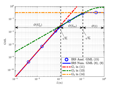
Figure 2: GML, $h_{\text{gml},3}$, vs. IRS length, $L$, for $w_{o1}=2.5$ mm.

In the following, we consider an FSO system with $\lambda=1550$ nm, $\zeta=1$, noise spectral density $N_{0}=-114\ \mathrm{dBm}/\mathrm{MHz}$, $\kappa=0.43\times 10^{-3}\frac{\mathrm{dB}}{\mathrm{m}}$, $C_{n}^{2}=50\times 10^{-15}$, $\eta=377\,\Omega$, $P_{\text{tot}}=1$ mW, $d_{3}=2$ km, $L_{\text{tr}}=1.6$ km, and $a=10$ cm [17]. We adopt a square-shaped IRS with $L_{x}=L_{y}=L$ and assume that the IRS and relay are centered at $(x_{o},z_{o})=(0,H_{e})$, respectively, unless specified otherwise. Fig. 2 shows the GML of the IRS-assisted FSO link, $h_{\text{gml,3}}$, versus the length of the IRS, $L$. As can be observed, the numerical GML in (10) and (11) matches the analytical approximation in (17). Moreover, depending on the IRS size, the analytical GML in (17) is determined by ${G}_{1}$ in (13), ${G}_{2}$ in (15), and $G_{3}$ in (16), where the dashed vertical lines indicate the boundary values $\sqrt{S_{1}}=1.13$ cm, and $\sqrt{S_{2}}=0.11$ m. Fig. 2 confirms that for an IRS length of $L\leq\sqrt{S_{1}}$, the GML ${G}_{1}$ increases quadratically with the IRS size $L^{2}$, see (13). By further increasing the IRS length, in the range $\sqrt{S_{1}}\leq L\leq\sqrt{S_{2}}$, the IRS collects the power of the tails of the Gaussian beam incident on the IRS and the GML scales linearly with the IRS size $L^{2}$. Finally, for IRS lengths of $L\geq\sqrt{S_{2}}$, due to the limited lens size, the IRS-based GML saturates to $G_{3}$ in (16).

Fig. 3 shows the outage probability of relay- and IRS-assisted FSO links for IRS lengths of $L=0.01$ m, $0.07$ m, and 1 m and a threshold SNR of $\gamma_{th}=0$ dB versus the transmit SNR, $\bar{\gamma}$. As can be observed, the analytical outage probabilities for the relay in (21) and the IRS in (19) match the simulation results. Furthermore, the asymptotic outage probability for IRS- and FSO-assisted links in (20) and (22), respectively, become accurate for high SNR values. As can be observed from Fig. 3, due to distance-dependent fading parameters, the diversity gain of the relay-assisted FSO link is approximately two times larger than that of the IRS-assisted link, i.e., $\frac{D_{\text{rel}}}{D_{\text{irs}}}=\frac{\min\{\varrho_{1},\varrho_{2}\}}{\varrho_{3}}=1.9$. Moreover, by increasing the IRS length from $0.01$ m to $0.07$ m, the FSO link gains 37.3 dB in SNR due to the linear scaling of the received power with the IRS size, see Fig. 2. However, when the IRS length increases from $0.07$ m to $1$ m, the received power saturates at a constant value and the additional SNR gain is only 9 dB. Furthermore, Fig. 3 reveals that for the adopted system parameters, an IRS with $L=1$ m outperforms the relay at low SNR values, although the performance difference is small.

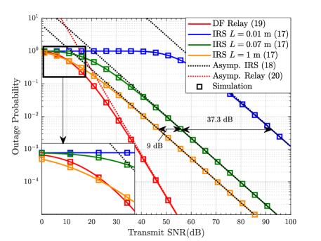
Figure 3: Outage probability vs. transmit SNR with $w_{o1}=w_{o2}=7$ mm and $\gamma_{th}=0$ dB.

Fig. 4 shows the outage probability of the IRS- and relay-assisted links for $\gamma_{th}=30$ dB versus the location of the center of the IRS/relay on the $x$-axis. To better illustrate the outage performance of extremely small IRSs, we also show results for $\gamma_{th}=-50$ dB. The optimal positions obtained from the analytical results in (24), (25) and simulations are denoted by ✶  and $\square$, respectively. The analytical outage probability for the relay-assisted link in (21) matches the simulation results. We obtained the outage probability for the IRS-assisted link in (19) based on GMLs $G_{1}$ in (12) , ${G}_{2}$ in (15), and $G_{3}$ in (16) for IRS sizes of $L=1$ mm, 3 cm, and 1 m, respectively. The analytical outage performance matches the simulation results except for an IRS length of $L=3$ cm. The reason is that the IRS with $L=3$ cm does not always operate in the linear power scaling regime, since the boundary values $S_{1}$ and $S_{2}$ in (17) change with the position of the IRS. However, despite the small discrepancy between simulation and analytical results for $x<-600$ m, the analytical optimal placement still leads to a close-to-optimal simulated outage performance. Furthermore, as can be observed, the optimal position of the relay is equidistant from Tx and Rx which matches the analytical result (25). Moreover, for different IRS sizes, different optimal positions are expected. For a small IRS length of $1$ mm, the IRS operates in the quadratic power scaling regime and the optimal location is close to the Tx or Rx. However, when the IRS size is large, i.e., $L=1$ m, the optimal position is equidistant from Tx and Rx . For IRSs with length $L=3$ cm, the optimal IRS position is close to the Tx as expected from (24).

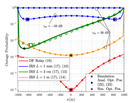
Figure 4: Outage probability vs. position of the $x$-coordinate of the center of IRS and relay with $w_{o1}=w_{o2}=7$ mm and $\bar{\gamma}=84$ dB.

VII Conclusions

In this paper, we analyzed the power scaling laws for IRS-assisted FSO systems. Depending on the beam waist, position of Tx and Rx w.r.t. the IRS, and lens radius, the received power at the lens grows quadratically or linearly with the IRS size or remains constant. We analyzed the GML, the boundary IRS sizes, and the asymptotic outage performance for these power scaling regimes. Our results show that, at the expense of higher hardware complexity, a relay-assisted link outperforms an IRS-assisted link at high SNR, although at low SNR the IRS-assisted link can be beneficial. We also compared the optimal IRS placement for the different power scaling regimes with the optimal relay placement. IRSs of small size achieve optimal outage performance close to the Tx (Rx), whereas large size IRSs perform better when placed equidistant from Tx and Rx.

Appendix A Proof of Lemma 1

First, for $L_{x}\ll w_{\text{in},x}$ and $L_{y}\ll w_{\text{in},y}$, the incident Gaussian beam on the IRS can be approximated by a plane wave as $\tilde{E}_{\text{in}}=\tilde{E}_{o}e^{-jk(d_{1}-x_{r}\cos(\theta_{i}))}$. To obtain $\tilde{E}_{o}$, we ensure that the powers of the plane wave and the Gaussian beam incident on the IRS are equal. Thus, $\frac{1}{2\eta}\iint_{\Sigma_{\text{irs}}}|\tilde{E}_{0}|^{2}\mathrm{d}x_{r}\mathrm{d}y_{r}=P_{\text{in}}$, where $P_{\text{in}}=\tilde{G}_{2}P_{\text{tot}}$ and $\tilde{G}_{2}$ is given in (2). This leads to $\tilde{E}_{o}=\sqrt{\frac{2\eta P_{\text{tot}}\tilde{G}_{2}\pi}{L_{x}L_{y}}}$. Then, given that $\Sigma_{\text{lens}}\ll A_{\text{rx}}$, we use the Huygens-Fresnel principle in (11) with the Taylor series approximation of $d_{2}\big{[}1+\frac{|\mathbf{r}_{p2}-\mathbf{r}_{r}|^{2}}{d_{2}^{2}}\big{]}^{1\over 2}\!\!\approx d_{2}-\frac{x_{r}(\sin(\theta_{r})x_{p2}+\cos(\theta_{r}))+y_{r}y_{p2}}{d_{2}}$, the reflected electric field is as follows

$${E}_{r}(\mathbf{r}_{p2})=\tilde{C}\text{sinc}\left(\frac{kL_{x}\sin(\theta_{r})}{2d_{2}}x_{p2}\right)\text{sinc}\left(\frac{kL_{y}}{2d_{2}}y_{p2}\right),\quad$$ (26)

where $\tilde{C}=L_{x}L_{y}\frac{\tilde{E}_{o}\sqrt{\sin(\theta_{r})}}{j\lambda d_{2}}e^{-jk\left(\Phi_{0}+d_{1}+d_{2}\right)}$. Then, we obtain

$$\int\text{sinc}^{2}(ax)\mathrm{d}x \overset{(a)}{=}\frac{-1}{2a^{2}x}\left[2ax\text{Si}(2ax)+\cos(2ax)-1\right],$$ (27)

where in $(a)$, we use the partial integration rule. Then, we approximate the circular lens of radius $a$ with a square lens of length $a\sqrt{\pi}$ [21] and substitute (26) in (10). Then, by applying (27), we obtain (12) and this completes the proof.

Appendix B Proof of Lemma 2

The electric field of the incident Gaussian beam on the IRS, $E_{\text{in}}({\mathbf{r}_{r}})$, is given by [9, Eq.(7)], thus, the incident power on the IRS, $P_{\text{in}}=\frac{1}{2\eta}\iint_{\Sigma_{\text{irs}}}\left|E_{\text{in}}({\mathbf{r}_{r}})\right|^{2}\mathrm{d}\mathbf{r}_{r}$, is given by

$$P_{\text{in}}=\frac{2P_{\text{tot}}\sin(\theta_{i})}{\pi w^{2}(d_{1})}\int_{-\frac{L_{x}}{2}}^{\frac{L_{x}}{2}}e^{-\frac{2x_{r}^{2}\sin^{2}(\theta_{i})}{w^{2}(d_{1})}}\mathrm{d}x_{r}\int_{-\frac{L_{y}}{2}}^{\frac{L_{y}}{2}}e^{-\frac{2y_{r}^{2}}{w^{2}(d_{1})}}\mathrm{d}y_{r}.\qquad$$ (28)

Then, we solve the above integral with [19, Eq. (2.33-2)]. As we assume the lens size in this case to be much smaller than the IRS size, the lens receives all the power incident on the IRS. Thus, the GML in this regime is obtained by normalizing (28) with $P_{\text{tot}}$, which leads to (14). This completes the proof.

Appendix C Proof of Lemma 3

The electric field reflected from the IRS and received at the lens, $E_{r}(\mathbf{r}_{p2})$, is given by [9, Eq. (16)]. Substituting $L_{x},L_{y}\to\infty$ in $E_{r}(\mathbf{r}_{p2})$, the GML in (10) becomes

$$G_{3}\!\!=\!\!C_{3}\int\limits_{-\frac{a\sqrt{\pi}}{2}}^{\frac{a\sqrt{\pi}}{2}}\!\!\!\!\!e^{-\frac{k^{2}\sin^{2}(\theta_{p})x_{p}^{2}\mathcal{R}\{b_{x}\}}{2d_{2}^{2}|b_{x}|^{2}}}\mathrm{d}x_{p2}\!\!\!\int\limits_{-\frac{a\sqrt{\pi}}{2}}^{\frac{a\sqrt{\pi}}{2}}e^{-\frac{k^{2}y_{p2}^{2}\mathcal{R}\{b_{y}\}}{2d_{2}^{2}|b_{y}|^{2}}}\mathrm{d}y_{p2},\qquad$$ (29)

where $C_{3}=\frac{2P_{\text{tot}}\sin(\theta_{i})\sin(\theta_{r})\pi}{\lambda^{2}w^{2}(d_{1})d_{2}^{2}|b_{x}||b_{y}|}$, $R\{\cdot\}$ denotes the real part of a complex number, $b_{x}=\frac{\sin^{2}(\theta_{i})}{w^{2}(d_{1})}-\frac{jk}{2}\left(\frac{\sin^{2}(\theta_{i})}{R(d_{1})}+{\sin^{2}(\theta_{r})\over d_{2}}\right)$, and $b_{y}=\frac{1}{w^{2}(d_{1})}-\frac{jk}{2}\left(\frac{1}{R(d_{1})}+{1\over d_{2}}\right)$. Then, substituting from [19, Eq. (2.33-2)], we obtain (16) and this completes the proof.

Appendix D Proof of Theorem 1

Depending on the IRS size, the optimal position of the IRS is calculated by approximating $h_{\text{gml},3}$ for each power scaling regime. First, the position of the center of the IRS $(x_{o},z_{o})$ on the ellipse can be rewritten in terms of $d_{1}$ and $d_{2}$ as follows

$$x_{o}=\frac{d_{1}^{2}-(d_{2})^{2}}{2L_{\text{tr}}},z_{o}=H_{e}\Big{[}1-\frac{\left(d_{1}^{2}-d_{2}^{2}\right)^{2}}{d_{3}^{2}L_{\text{tr}}^{2}}\Big{]}^{1/2}.\quad$$ (30)

For $\Sigma_{\text{irs}}\leq S_{1}\vee\Sigma_{\text{irs}}\leq S_{3}$, the GML is $h_{\text{gml},3}\approx{G}_{1}$. Then, we substitute in (13), the values of $\sin(\theta_{i})=\frac{z_{o}}{d_{1}}$, $\sin(\theta_{p})=\frac{z_{o}}{d_{p}}$, $z_{o}$ given in (30), and $d_{2}=d_{3}-d_{1}$. Next, by solving $\frac{\mathrm{d}{G}_{1}}{\mathrm{d}d_{1}}=0$, the extremal points, comprising maxima and minima, are given by

$$d_{1,\text{min}}^{(1)}=\frac{d_{3}}{2},\,d_{1,\text{max}}^{(2)}=\frac{d_{3}}{2}+\frac{\sqrt{2\rho_{1}}}{4},\, d_{1,\text{max}}^{(3)}=\frac{d_{3}}{2}-\frac{\sqrt{2\rho_{1}}}{4}.\qquad$$ (31)

Then, substituting the maxima in (30) leads to (24).

Next, for $S_{1}\leq\Sigma_{\text{irs}}\leq S_{2}$, the GML is $h_{\text{gml},3}\approx{G}_{2}$. Then, we substitute $\sin(\theta_{i})=\frac{z}{d_{1}}$ and $d_{2}=d_{3}-d_{1}$ in (15). Then, by solving $\frac{{G}_{2}}{\mathrm{d}d_{1}}=0$, the extremal points are given by

$$d_{1,\text{max}}^{(1)}=\left(5d_{3}+\sqrt{\rho_{2}}\right)/8,\quad d_{1,\text{max}}^{(2)}=\left(5d_{3}-\sqrt{\rho_{2}}\right)/8.$$ (32)

Here, $d_{1,\text{max}}^{(1)}$ does not lie on the ellipse, since $d_{1,\text{max}}^{(1)}>\max(d_{1})$, where $\max(d_{1})=\frac{d_{3}+L_{\text{tr}}}{2}$. Then, substituting $d_{1,\text{max}}^{(2)}$ in (30) leads to (24).

Next, for $\Sigma_{\text{irs}}>S_{2}\vee\Sigma_{\text{irs}}>S_{3}$, the GML is $h_{\text{gml},3}\approx G_{3}$. Then, assuming $d_{1}\gg z_{R1}$, we substitute $w(d_{1})\approx\frac{\lambda d_{1}}{\pi w_{o1}}$, $R(d_{1})=d_{1}$, and $d_{2}=d_{3}-d_{1}$ in (16). The maximum of the $\text{erf}(\cdot)$ functions in (16) occur for the minimum of the beamwidths $W_{\text{eq},x}$ and $W_{\text{eq},x}$. By solving $\frac{\mathrm{d}W_{\text{eq},i}}{\mathrm{d}d_{1}}=0,i\in\{x,y\}$, we obtain similar minimal points at $\frac{d_{3}}{2}$. Thus, both $\text{erf}(\cdot)$ functions in (16) are maximized at $\frac{d_{3}}{2}$, which in turn maximizes $G_{3}$. Substituting $\frac{d_{3}}{2}$ in (30) leads to (24) and this completes the proof.

References

• [1] W. Saad, M. Bennis, and M. Chen, “A vision of 6G wireless systems: Applications, trends, technologies, and open research problems,” IEEE Network, vol. 34, no. 3, pp. 134–142, May/June 2020.
• [2] M. Safari and M. Uysal, “Relay-assisted free-space optical communication,” IEEE Trans. Wireless Commun., vol. 7, pp. 5441–5449, Dec. 2008.
• [3] M. Najafi and R. Schober, “Intelligent reflecting surfaces for free space optical communications,” in Proc. IEEE Globecom, 2019.
• [4] M. Najafi, B. Schmauss, and R. Schober, “Intelligent reflecting surfaces for free space optical communication systems,” IEEE Trans. Commun., vol. 69, no. 9, pp. 6134–6151, 2021.
• [5] A. R. Ndjiongue, T. M. N. Ngatched, O. A. Dobre, and H. Haas, “Design of a power amplifying-RIS for free-space optical communication systems,” IEEE Wireless Commun., vol. 28, no. 6, pp. 152–159, 2021.
• [6] S. Kazemlou, S. Hranilovic, and S. Kumar, “All-optical multihop free-space optical communication systems,” J. Lightwave Technology, vol. 29, no. 18, pp. 2663–2669, 2011.
• [7] M. Di Renzo, A. Zappone, M. Debbah, M.-S. Alouini, C. Yuen, J. de Rosny, and S. Tretyakov, “Smart radio environments empowered by reconfigurable intelligent surfaces: How it works, state of research, and the road ahead,” IEEE J. Sel. Areas Commun., vol. 38, no. 11, pp. 2450–2525, Nov. 2020.
• [8] A. R. Ndjiongue, T. M. N. Ngatched, O. A. Dobre, A. G. Armada, and H. Haas, “Analysis of RIS-based terrestrial-FSO link over G-G turbulence with distance and jitter ratios,” J. Lightwave Technology, vol. 39, no. 21, pp. 6746–6758, 2021.
• [9] H. Ajam, M. Najafi, V. Jamali, B. Schmauss, and R. Schober, “Modeling and design of IRS-assisted multi-link FSO systems,” IEEE Trans. Commun., pp. 1–1, 2022.
• [10] Q. Wu and R. Zhang, “Intelligent reflecting surface enhanced wireless network via joint active and passive beamforming,” IEEE Trans. Wireless Commun., vol. 18, no. 11, pp. 5394–5409, 2019.
• [11] E. Björnson and L. Sanguinetti, “Power scaling laws and near-field behaviors of massive MIMO and intelligent reflecting surfaces,” IEEE Open Journal of the Communications Society, vol. 1, pp. 1306–1324, 2020.
• [12] V. Jamali, H. Ajam, M. Najafi, B. Schmauss, R. Schober, and H. V. Poor, “Intelligent reflecting surface assisted free-space optical communications,” IEEE Commun. Mag., vol. 59, no. 10, pp. 57–63, 2021.
• [13] E. Björnson, O. Özdogan, and E. G. Larsson, “Intelligent reflecting surface versus decode-and-forward: How large surfaces are needed to beat relaying?” IEEE Wireless Communications Letters, vol. 9, no. 2, pp. 244–248, 2020.
• [14] C. Huang, A. Zappone, G. C. Alexandropoulos, M. Debbah, and C. Yuen, “Reconfigurable intelligent surfaces for energy efficiency in wireless communication,” IEEE Trans. Wireless Commun.,, vol. 18, no. 8, pp. 4157–4170, 2019.
• [15] S. Molla Aghajanzadeh and M. Uysal, “Performance analysis of parallel relaying in free-space optical systems,” IEEE Trans. Commun., vol. 63, no. 11, pp. 4314–4326, 2015.
• [16] M. A. Kashani, M. Safari, and M. Uysal, “Optimal relay placement and diversity analysis of relay-assisted free-space optical communication systems,” J. Optical Commun. and Networking, vol. 5, no. 1, pp. 37–47, 2013.
• [17] H. Ajam, M. Najafi, V. Jamali, and R. Schober, “Channel modeling for IRS-assisted FSO systems,” in Proc. IEEE WCNC, 2021, pp. 1–7.
• [18] L. Yang, X. Gao, and M. Alouini, “Performance analysis of free-space optical communication systems with multiuser diversity over atmospheric turbulence channels,” IEEE Photonics Journal, vol. 6, no. 2, pp. 1–17, Apr. 2014.
• [19] I. S. Gradshteyn and I. M. Ryzhik, Table of Integrals, Series, and Products.   San Diego, CA: Academic, 1994.
• [20] J. W. Goodman, Introduction to Fourier Optics.   Roberts & Co., 2005.
• [21] A. A. Farid and S. Hranilovic, “Outage capacity optimization for free-space optical links with pointing errors,” J. Lightwave Technology, vol. 25, no. 7, pp. 1702–1710, 2007.
• [22] M. Najafi, V. Jamali, R. Schober, and H. V. Poor, “Physics-based modeling and scalable optimization of large intelligent reflecting surfaces,” IEEE Trans. Commun., vol. 69, no. 4, pp. 2673–2691, 2021.
• [23] Q. Tao, J. Wang, and C. Zhong, “Performance analysis of intelligent reflecting surface aided communication systems,” IEEE Commun. Lett., vol. 24, no. 11, pp. 2464–2468, 2020.