Bivariate vine copula based regression, bivariate level and quantile curves

Abstract

The statistical analysis of univariate quantiles is a well developed research topic. However, there is a need for research in multivariate quantiles. We construct bivariate (conditional) quantiles using the level curves of vine copula based bivariate regression model. Vine copulas are graph theoretical models identified by a sequence of linked trees, which allow for separate modelling of marginal distributions and the dependence structure. We introduce a novel graph structure model (given by a tree sequence) specifically designed for a symmetric treatment of two responses in a predictive regression setting. We establish computational tractability of the model and a straight forward way of obtaining different conditional distributions. Using vine copulas the typical shortfalls of regression, as the need for transformations or interactions of predictors, collinearity or quantile crossings are avoided. We illustrate the copula based bivariate level curves for different copula distributions and show how they can be adjusted to form valid quantile curves. We apply our approach to weather measurements from Seoul, Korea. This data example emphasizes the benefits of the joint bivariate response modelling in contrast to two separate univariate regressions or by assuming conditional independence, for bivariate response data set in the presence of conditional dependence.

Keyword: multivariate quantiles, bivariate response, bivariate conditional distribution functions

1 Introduction

The topic of predicting quantiles of a response variable conditioned on a set of predictor variables taking on fixed values, continuously attracts interest. The statistical analysis of such univariate quantiles is a well developed research topic (Koenker and Bassett, 1978; Koenker, 2005). Since the introduction of the linear quantile regression by Koenker and Bassett, (1978) many extensions have been developed for the case of a univariate response variable. A short summary of developments in quantile regression modelling is given in Koenker, (2017). Recent approaches for quantile regression are vine copula based quantile regression methods (Kraus and Czado, 2017; Tepegjozova et al., 2022; Chang and Joe, 2019; Zhu et al., 2021). Copulas allow for separate modelling of the marginal distributions and the dependence structure in the data. Vine copulas construct multivariate copulas using bivariate building blocks only, a so-called pair copula construction. This way, a very flexible model, without assuming homoscedasticity, or a linear relationship between the response and the predictors, is constructed. Thus, vine based quantile regression methods overcome two drawbacks of the standard quantile regression methods. First, by construction quantile crossings and collinearity are avoided, and second, there is no need for transformations or interactions of variables (Kraus and Czado, 2017). There are several different vine copula tree structures that can be considered, the most general regular (R-)vine copulas, or subsets such as drawable (D-vines whose tree structure is a sequence of paths) and canonical (C-vines whose tree structure is a sequence of stars) vines. Kraus and Czado, (2017) developed a parametric D-vine based quantile regression method by optimizing the conditional log-likelihood and adding predictors until there is no improvement, thus introducing an automatic forward variable selection method. This approach was extended in Tepegjozova et al., (2022) where a nonparametric D- and C-vine copula based quantile regression was introduced. They also follow the approach to maximize the conditional log likelihood, but introduce an additional step to check for future improvement of the conditional log likelihood, a so called two-step ahead approach. Chang and Joe, (2019) introduced R-vine based quantile regression model by first finding the optimal R-vine structure among all predictors and then adding the response variable to each tree in the vine structure as a leaf node. Another R-vine based regression was introduced in Zhu et al., (2021) by choosing the R-vine structure which gives the largest sum of the absolute value of the partial correlations in each step of the forward extension with predictor variables, while keeping the response as a leaf node. This approach is motivated by the algorithm and results from Zhu et al., (2020). All these selected structures allow to express the conditional density of the response given the predictors without integration.

Despite the great attention univariate quantiles have received, the extension to multivariate response quantiles is not trivial nor well-defined. Several theoretical notions of multivariate quantiles have been introduced, but there is no consensus which one is the corresponding generalization of the univariate quantiles. These include geometric quantiles based on halfspace depth contours with different concepts of statistical depth (e.g. see Tukey, (1975), Chaudhuri, (1996), Hallin et al., (2010), Chernozhukov et al., (2017)), vector quantiles (see Carlier et al., (2016) and Carlier et al., (2017)), spatial quantiles (see Abdous and Theodorescu, (1992)). Our goal is to define bivariate quantiles in terms of copula distribution and to introduce a vine based regression method able to handle bivariate responses. Copula based models are known to be excelling at modeling tail events and asymmetric dependencies. Bivariate quantiles arising from copula based models are advantageous in assessing the joint risk of failure or occurrence of two events. One example of specific bivariate quantiles being applied is the analysis of floods by Chebana and Ouarda, (2011). The risk of flood is studied through a joint analysis of flood peaks and flood volumes, using level sets of bivariate copulas. Requena et al., (2013) present a similar analysis of the risk of flood, focusing on hydrologic dam designs. Additionally, the authors use the same approach for a joint analysis of reservoir volume and spillway crest length as indicators for the risk of dam overtopping. A multivariate risk of failure analysis based on copulas is presented in Salvadori et al., (2015) for structural failure assessment in engineering. An application in financial mathematics can be found in Di Bernardino and Prieur, (2014). The authors propose estimation of a tail event risk measure based on multivariate level sets of copulas. However, all these approaches model the two responses with a copula, but do not consider any explanatory variables or predictors. It would be even more beneficial to jointly model two response variables, taking into account the influence of a set of possible predictors. Thus, to fill in this gap, we focus on bivariate conditional quantiles and their estimation using a very flexible vine copula model.

The first heuristic for a vine based quantile regression with multiple responses is given in Zhu et al., (2021), but the question of multivariate response quantiles is not tackled. The suggested heuristic for the bivariate response case is limited to modelling only, but not predicting the bivariate quantiles. Further, this approach has an asymmetric treatment of the response variables. This might lead to different performance of the regression methods when the order of the response variables is exchanged. Thus, there is still a need for: $(1.)$ a valid definition of (unconditional and conditional) multivariate quantiles linked to the usage of copulas; $(2.)$ a vine based quantile regression method with a symmetric treatment of the responses; $(3.)$ a numerical method for obtaining the multivariate (unconditional and conditional) quantiles from the estimated vine based model and evaluating predictions from it.

Our methodology deals with the case of a bivariate response variables, i.e. bivariate (unconditional and conditional) quantiles defined by sets that can be characterised as curves. For the conditional case we choose the multivariate vine copulas class since they allow modelling of complex dependence patterns including asymmetric tail dependencies. For $(1.)$ we extend the definition of bivariate unconditional and conditional quantiles in terms of a copula distribution function. We first start by exploring (un)conditional level curves of copula distributions. Further, we illustrate the bivariate unconditional level curves for known bivariate copula distributions and the bivariate conditional level curves for a 3-dimensional vine copula distribution. Then, we show that the coverage probabilities of the $\alpha$ level curves is not $\alpha$ and propose to adjust them in such a way that the adjusted level, say $\beta(\alpha)$ results in bivariate quantile curves with coverage $\alpha$. For $(2.)$, we propose a novel tree structure for vines, called Y-vine tree sequence, which is contained in the set of regular vine tree sequences. It is designed to allow for a symmetric treatment of the responses. Moreover, we show that using the Y-vine tree sequence the associated bivariate conditional density is analytically expressible as a product of all pair copula terms involving one or both of the response variables. In the case of more than one conditioning variable (predictor) we develop a forward selection method. For this we propose an appropriate fit measure for the selection of predictors to prevent overfitting and remove non-significant predictors. For $(3.)$ we develop a numerical method to evaluate the bivariate unconditional and conditional level curves and corresponding quantile curves. Based on the estimated quantiles, we can construct bivariate confidence regions, which is a generalization of univariate confidence intervals. They contain the data with a given probability and can locate parts of a distribution with high density values. Such confidence regions can be effective for visualizing trends, patterns and outliers (Korpela et al., 2014, 2017; Guilbaud, 2008). Further, for applicability of the proposed method we develop a prediction method of the two responses given an arbitrary set of predictor values and show how to simulate data from a Y-vine with fixed predictor values. Finally, we give an application involving a data set with minimal and maximal daily temperatures together with other weather variables. For this application we show that the conditional dependence cannot be ignored and that it is non-Gaussian, thus requiring the full class of pair copula families. In addition, we illustrate our confidence regions and compare them to alternative ways of construction of confidence regions, assuming (conditional) independence. We highlight the advantages of our modeling approach and its usability in data analysis.

The remainder of the paper is organized as follows. First, we introduce the necessary vine copula concepts for our approach in Section 2. In Section 3 we introduce the Y-vine copula based regression model for bivariate responses. For application purposes, in Section 4 we present the prediction method for Y-vine copulas. Then, in Section 5 we define bivariate level curves and quantile curves in terms of copulas and develop numerical methods used for their evaluation. For the demonstration of the usefulness of our method we include a real data example in Section 6 that contains dependent bivariate responses. We highlight the advantages of bivariate response modelling over standard univariate models or models that assume conditional independence. Finally, in Section 7 we give conclusions and areas of future research.

2 Theoretical background

Consider any continuous d-dimensional random vector $\mathbf{X}=\left(X_{1},\ldots,X_{d}\right)^{T}$ with observed values $\mathbf{x}=\left(x_{1},\ldots,x_{d}\right)^{T}$. We use capital letters for random variables and lowercase letters for their observed values, i.e., we write $X_{i}=x_{i}$ for $i=1,\ldots,d$. Let $\mathbf{X}$ have joint distribution function $F$, joint density $f$ and marginal distributions $F_{X_{i}},\;i=1,\ldots,d.$ Following Sklar’s theorem (Sklar, 1959), we can express the multivariate distribution function $F$ in terms of the marginal distributions, $F_{X_{i}}$, and the $d$-dimensional copula $C$ as

$$F\left(x_{1},\ldots,x_{d}\right)=C\left(F_{X_{1}}(x_{1}),\ldots,F_{X_{d}}(x_{d})\right).$$ (1)

Since we assume a continuous joint distribution $F$, the copula $C:\left[0,1\right]^{d}\mapsto\left[0,1\right]$ corresponds to the distribution of the random vector $\mathbf{U}=\left(U_{1},\ldots,U_{d}\right)^{T},$ with the components of $\mathbf{U}$ being the probability integral transforms (PITs or u-scale) of the components of $\mathbf{X}$ (x-scale), $U_{i}=F_{X_{i}}\left(X_{i}\right)$ for $i=1,\ldots,d$. Each $U_{i}$ is uniformly distributed and their joint distribution function $C$ is the copula associated with $\mathbf{X}$. By Sklar’s Theorem it is implied that $C$ is unique, in the absolutely continuous case, which we assume. Also, if derivatives of the marginal distributions $F_{X_{i}}$ exist, the density $f$ can be derived as

$$f\left(x_{1},\ldots,x_{d}\right)=c\left(F_{X_{1}}(x_{1}),\ldots,F_{X_{d}}(x_{d})\right)\cdot\prod_{i=1}^{d}f_{X_{i}}\left(x_{i}\right),$$ (2)

where $c$ is the $d$-dimensional density corresponding to the copula $C$ and $f_{X_{1}},\ldots,f_{X_{d}}$ are the univariate marginal densities. However, Equations 1 and 2 both incorporate a possibly complicated multivariate copula distribution and density. As shown by Joe, (1996), a $d$-dimensional copula density can be decomposed into $d\left(d-1\right)/2$ bivariate copula densities. This decomposition is not unique, but a large number of possible decompositions exist. The elements of these decompositions, the bivariate copula densities can be chosen completely independent of each other. A graphical model introduced by Bedford and Cooke, (2002), called regular vine copulas (R-vines), organizes all such decompositions that lead to a valid density. Thus, the estimation of a $d$-dimensional copula density is subdivided into the estimation of $d(d-1)/2$ two-dimensional copula densities. A regular vine copula on $d$ uniformly distributed random variables $U_{1},\ldots,U_{d},$ consists of a regular vine tree sequence, denoted by $\mathcal{V}$, a set of bivariate copula families (also known as pair copulas) $\mathcal{B}\left(\mathcal{V}\right)$, and a set of parameters corresponding to the bivariate copula families $\Theta\left(\mathcal{B}\left(\mathcal{V}\right)\right)$. The vine tree sequence or tree structure $\mathcal{V}$ consists of a sequence of linked trees, $T_{k}=\left(N_{k},E_{k}\right),\;k=1,\ldots,d-1$, satisfying the following conditions:

• $T_{1}$ is a tree with node set $N_{1}=\left\{U_{1},\ldots,U_{d}\right\}$ and edge set $E_{1}$.

• For $k\geq 2$, $T_{k}$ is a tree with node set $N_{k}=E_{k-1}$ and edge set $E_{k}$.

• (Proximity condition) For $k\geq 2$, two nodes of the tree $T_{k}$ can be connected by an edge if the corresponding edges of $T_{k-1}$ have a common node.

If the vine tree sequence consists of paths only, then we call it a drawable vine (D-vine), and if it consists of stars, it is called a canonical vine (C-vine) (Bedford and Cooke, 2002). The tree sequence uniquely specifies which bivariate (conditional) copula densities occur in the decomposition. Each edge $e\in E_{k}$ for $k=1,\ldots,d-1$ is associated with a bivariate copula family $c_{U_{j_{e}},U_{k_{e}};\mathbf{U}_{D_{e}}}\in\mathcal{B}\left(\mathcal{V}\right),$ and a corresponding set of parameters $\bm{\theta}_{j_{e},k_{e};D_{e}}\in\Theta\left(\mathcal{B}\left(\mathcal{V}\right)\right)$. $U_{j_{e}}$ and $U_{k_{e}}$ are the conditioned variables and $\mathbf{U}_{D_{e}}$ represents the conditioning set corresponding to edge $e$, $\mathbf{U}_{D_{e}}=\left(U_{i}\right)_{i\in D_{e}}$. Denote the conditional distribution of $U_{j_{e}}|\mathbf{U}_{D_{e}}=\mathbf{u}_{D_{e}}$ with $C_{U_{j_{e}}|\mathbf{U}_{D_{e}}}$. We define the so-called pseudo copula data $u_{j_{e}|D_{e}}$ as $u_{j_{e}|D_{e}}\coloneqq C_{U_{j_{e}}|\mathbf{U}_{D_{e}}}\left(u_{j_{e}}|\mathbf{u}_{D_{e}}\right)$. Similarly, $u_{k_{e}|D_{e}}$ is defined. Then, $c_{U_{j_{e}},U_{k_{e}};\mathbf{U}_{D_{e}}}$ denotes the density of the copula between the pseudo copula data $u_{j_{e}|D_{e}}$ and $u_{k_{e}|D_{e}}$. The corresponding distribution function is denoted as $C_{U_{j_{e}},U_{k_{e}};\mathbf{U}_{D_{e}}}$.

Bedford and Cooke, (2002) have shown that the graphical model of regular vines, leads to a natural decomposition of the joint copula density $c$ using the pair-copulas defined through the tree sequence as

$$c\left(u_{1},\ldots,u_{d}\right)=\prod_{k=1}^{d-1}\prod_{e\in E_{k}}c_{U_{j_{e}},U_{k_{e}};\mathbf{U}_{D_{e}}}\left(C_{U_{j_{e}}|\mathbf{U}_{D_{e}}}\left(u_{j_{e}}|\mathbf{u}_{D_{e}}\right),C_{U_{k_{e}}|\mathbf{U}_{D_{e}}}\left(u_{k_{e}}|\mathbf{u}_{D_{e}}\right)|\mathbf{u}_{D_{e}}\;\right).$$ (3)

Using Equation 3 we can decompose any given regular vine copula density. However, the individual pair copulas, $c_{U_{j_{e}},U_{k_{e}};\mathbf{U}_{D_{e}}}$ in Equation  3 are dependent on $\mathbf{u}_{D_{e}}$. This represents the different conditional dependencies between $U_{j_{e}}$ and $U_{k_{e}}$ for different conditioning values of $\mathbf{u}_{D_{e}}$. To improve computational tractability, it is customary to ignore this influence and simplify Equation 3 to:

$$c\left(u_{1},\ldots,u_{d}\right)=\prod_{k=1}^{d-1}\prod_{e\in E_{k}}c_{U_{j_{e}},U_{k_{e}};\mathbf{U}_{D_{e}}}\left(C_{U_{j_{e}}|\mathbf{U}_{D_{e}}}\left(u_{j_{e}}|\mathbf{u}_{D_{e}}\right),C_{U_{k_{e}}|\mathbf{U}_{D_{e}}}\left(u_{k_{e}}|\mathbf{u}_{D_{e}}\right)\;\right).$$ (4)

This simplification is known as the simplifying assumption (more in Haff et al., (2010) and Stoeber et al., (2013)). It is made due to tractability in higher dimensions, and can be further tested for validity (see for example Kurz and Spanhel, (2022) and Derumigny and Fermanian, (2017)). In this case, we talk about pair copula constructions (PCC) of multivariate densities.
To derive the conditional distributions in Equation 4, we use the recursion formula from Joe, (1996). It defines a recursion for conditional distributions of a regular vine over its tree sequence. Let $l\in D_{e}$ and $D_{-l}\coloneqq D_{e}\setminus\left\{l\right\}$. Further, let $h_{U_{j_{e}}|U_{l};\mathbf{U}_{D_{-l}}}\left(\cdot|\cdot\right)$ denote the so-called h-function associated with the pair copula $c_{U_{j_{e}},U_{l};\mathbf{U}_{D_{-l}}}$, defined as $h_{U_{j_{e}}|U_{l};\mathbf{U}_{D_{-l}}}(u_{j_{e}}|u_{l})\coloneqq\frac{\partial}{\partial u_{l}}C_{U_{j_{e}},U_{l};\mbox{\boldmath$U$}_{D_{-l}}}(u_{j_{e}},u_{l}).$ Then the following recursion is valid

$$C_{U_{j_{e}}|\mathbf{U}_{D_{e}}}\left(u_{j_{e}}|\mathbf{u}_{D_{e}}\right)=h_{U_{j_{e}}|U_{l};\mathbf{U}_{D_{-l}}}\left(C_{U_{j_{e}}|\mathbf{U}_{D_{-l}}}\left(u_{j_{e}}|\mathbf{u}_{D_{-l}}\right)|C_{U_{l}|\mathbf{u}_{D_{-l}}}\left(u_{l}|\mathbf{U}_{D_{-l}}\right)\right).$$ (5)

3 Vine copula based bivariate regression

3.1 General framework

Consider the variables $(Y_{1},Y_{2})^{T}$ as the 2-dimensional response vector and $\mathbf{X}=\left(X_{1},\ldots,\right.$ $\left.X_{p}\right)^{T}$ as the p-dimensional predictor vector. The main interest of the bivariate regression is to model the joint conditional distribution function of the response variables $\mathbf{Y}=\left(Y_{1},Y_{2}\right)^{T}$ given the outcome of some predictor variables $\mathbf{X}=\mathbf{x}$, denoted as $F_{Y_{1},Y_{2}|\mathbf{X}}\left(y_{1},y_{2}|\mathbf{x}\right)$. This can be achieved by joint modelling of $\left(\mathbf{Y},\mathbf{X}\right)^{T}$ and subsequently deriving the conditional distribution of the bivariate response vector $\mathbf{Y}$ given $\mathbf{X}=\mathbf{x}$. The same can be achieved by joint modelling of the PIT values of the responses $\mathbf{V}=\left(V_{1},V_{2}\right)^{T}$, the predictors $\mathbf{U}=\left(U_{1},\ldots,U_{p}\right)^{T},$ and the corresponding conditional distribution function of $\mathbf{V}$ given $\mathbf{U}=\mathbf{u}$, denoted as $C_{V_{1},V_{2}|\mathbf{U}}\left(v_{1},v_{2}|\mathbf{u}\right)$. The connection between these two approaches for the joint conditional distribution, on the x- and u-scale, is derived in Proposition 3.1.

Proposition .

The conditional distribution of $\mathbf{Y}=\left(Y_{1},Y_{2}\right)^{T}$ given $\mathbf{X}=\left(X_{1},\ldots,X_{p}\right)^{T},$ with corresponding PITs $V_{j}\coloneqq F_{Y_{j}}\left(Y_{j}\right),\;j=1,2$ and $U_{i}\coloneqq F_{X_{i}}\left(X_{i}\right),\;i=1,\ldots,p$ can be expressed in terms of a conditional distribution function associated with a copula as

$$F_{Y_{1},Y_{2}|\mathbf{X}}\left(y_{1},y_{2}|\mathbf{x}\right)=C_{V_{1},V_{2}|\mathbf{U}}\left(F_{Y_{1}}(y_{1}),F_{Y_{2}}(y_{2})|F_{X_{1}}(x_{1}),\ldots,F_{X_{p}}(x_{p})\right).$$

Proof of Proposition 3.1 is given in Appendix B.1. Here $C_{V_{1},V_{2}|\mathbf{U}}$ is the bivariate conditional distribution associated with the $p+2$ dimensional copula $C_{V_{1},V_{2},\mathbf{U}}$ and does not need to have uniform margins. In general, $C_{V_{1},V_{2}|\mathbf{U}}$ is different than $C_{V_{1},V_{2};\mathbf{U}}$, as $C_{V_{1},V_{2};\mathbf{U}}$ is a bivariate copula with uniform marginal distributions and corresponds to the copula associated with the bivariate conditional distribution of $(Y_{1},Y_{2})$ given $\mathbf{X}=\mathbf{x}$. From Proposition 3.1, in order to model the bivariate conditional distribution function, we need to estimate the marginal distributions $F_{Y_{j}},F_{X_{i}}$ for $j=1,2,\;i=1,\ldots,p,$ and the bivariate conditional distribution $C_{V_{1},V_{2}|\mathbf{U}}$. To obtain the later, we need to estimate the $p+2$ dimensional copula $C_{V_{1},V_{2},\mathbf{U}}$ describing the joint distribution of $(V_{1},V_{2},\mathbf{U})$. Following Kraus and Czado, (2017); Noh et al., (2013), we estimate the marginal distributions nonparameterically to reduce the bias caused by model misspecification. Examples of nonparametric univariate estimators are the continuous kernel smoothing estimator (Parzen, 1962) and the transformed local likelihood estimator (Geenens, 2014). A more complex task is estimating the $p+2$ dimensional copula $C_{V_{1},V_{2},\mathbf{U}}$ and subsequently, deriving the bivariate conditional distribution from this copula. We propose to model the copula $C_{V_{1},V_{2},\mathbf{U}}$ using regular vine copulas. However, we also have to take care that deriving the bivariate conditional distribution $C_{V_{1},V_{2}|\mathbf{U}}$ remains numerically tractable. Thus, to obtain the joint conditional distribution of the response variables using only pair copulas estimated in the vine copula model, additional constraints are required. The constraint for a univariate vine regression is that the node containing the response in the conditioned set is a leaf node in each tree of the tree sequence, as shown by Kraus and Czado, (2017) for D-vines and by Tepegjozova et al., (2022) for C-vines. Following these results, the constraint for the bivariate vine regression model is that the two response variables are exactly the conditioned set of the edge of the last tree in the vine tree sequence, as also used by Zhu et al., (2021). However, in their approach there is no symmetric treatment of the two responses, which is a drawback. Therefore, we propose a new vine tree structure specifically designed for bivariate regression modelling with a symmetric treatment of the responses.

3.2 Y-vine copula model

Let $\mathbf{X}_{-i}$ be a $(p-1)$-dimensional vector defined as $\mathbf{X}_{-i}\coloneqq(X_{1},\ldots,X_{i-1},X_{i+1},\ldots X_{p})^{T}$ and let $\mathbf{X}_{i:i+k}$ be a $(k+1)$-dimensional vector defined as $\mathbf{X}_{i:i+k}\coloneqq(X_{i},\ldots,X_{i+k})^{T}.$ Similar definitions hold for the vectors $\mathbf{x}_{-i},\mathbf{U}_{-i}$, $\mathbf{u}_{-i}$, and for $\mathbf{x}_{i:i+k},\mathbf{U}_{i:i+k}$ $\mathbf{u}_{i:i+k}$, respectively.

Definition .

Given the marginal PIT transformed response variables $V_{1},V_{2}$ and predictor variables $U_{1},\ldots,U_{p}$, we define the $p+1$ trees of the Y-vine tree sequence for bivariate regression as the following:

• with $N_{1}=\left\{V_{1},V_{2},U_{1},\ldots,U_{p}\right\}$ and $E_{1}=\left\{\left(V_{1},U_{1}\right),\;\left(V_{2},U_{1}\right)\right\}\;\bigcup_{i=1}^{p-1}\left(U_{i},U_{i+1}\right).$

• with $N_{2}=\left\{V_{1}U_{1},V_{2}U_{1},U_{1}U_{2},\ldots,U_{p-1}U_{p}\right\}$ and
  $E_{2}=\left\{\left(V_{1}U_{1},\;U_{1}U_{2}\right),\;\left(V_{2}U_{1},\;U_{1}U_{2}\right)\right\}\;\bigcup_{i=1}^{p-2}\left(U_{i}U_{i+1},\;U_{i+1}U_{i+2}\right).$

• for $3\leq k\leq p$ with $N_{k}=\bigcup_{j=1,2}\left\{V_{j}U_{k-1};\mathbf{U}_{1:k-2}\right\}\bigcup_{i=1}^{p-k+1}\left\{U_{i}U_{i+k-1};\mathbf{U}_{i+1:i+k-2}\right\}$
  and $E_{k}=\bigcup_{j=1,2}\left\{\left(V_{j}U_{k-1};\mathbf{U}_{1:k-2},\;\;U_{1}U_{k};\mathbf{U}_{2:k-1}\right)\right\}$
            $\;\;\quad\bigcup_{i=1}^{p-k}\left\{\left(U_{i}U_{i+k-1};\mathbf{U}_{i+1:i+k-2},\;\;U_{i+1}U_{i+k};\mathbf{U}_{i+2:i+k-1}\right)\right\}.$

• with $N_{p+1}=\bigcup_{j=1,2}\left\{V_{j}U_{p};\mathbf{U}_{1:p-1}\right\}$ and $E_{p+1}=\left\{\left(V_{1}U_{p};\mathbf{U}_{1:p-1},\;\;V_{2}U_{p};\mathbf{U}_{1:p-1}\right)\right\}.$

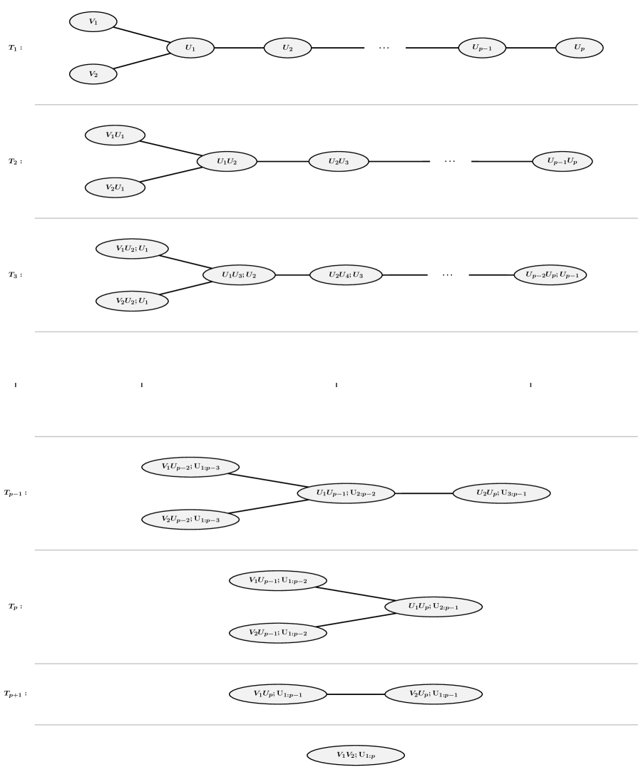
Figure 1: Y-vine tree sequence on the u-scale.

The newly proposed Y-vine tree sequence is illustrated in Figure 1. In each tree of the vine tree sequence the nodes containing the predictor variables in the conditioned set are arranged in a path, while the nodes containing the response variables in the conditioned set are added as leafs of the path on one end. The subset of the sequence that contains a single response and all predictors forms a D-vine tree sequence. This tree structure allows for symmetric treatment of the response variables, especially important since an asymmetric treatment might lead to different performances of the regression models depending on the order. The proposed Y-vine tree sequence satisfies the regular vine tree sequence conditions $(i)$-$(iii)$ from Section 2 and thus, represents a valid regular vine tree sequence. The proof is provided in the supplementary material.

A regular vine copula associated with a $Y$-vine tree sequence together with a set of bivariate copulas $\mathcal{B}\left(\mathcal{V}\right)$ and the corresponding pair copula parameters $\Theta\left(\mathcal{B}\left(\mathcal{V}\right)\right)$ is called a $Y$-vine copula and we denote it by $\mathcal{Y}$. The joint density $f_{Y_{1},Y_{2},\mathbf{X}}$ using a $Y$-vine tree sequence can be expressed by Equation4 as

$$\begin{split}f_{Y_{1},Y_{2},\mathbf{X}}&\left(y_{1},y_{2},\mathbf{x}\right)=\prod_{k=1}^{p-1}\left[\prod_{i=1}^{p-k}c_{U_{i},U_{i+k};\mathbf{U}_{i+1:i+k-1}}\left(F_{X_{i}|\mathbf{X}_{i+1:i+k-1}}(x_{i}|\mathbf{x}_{i+1:i+k-1}),\right.\right.\\ &\hskip 187.78836pt\left.F_{X_{i+k}|\mathbf{X}_{i+1:i+k-1}}(x_{i+k}|\mathbf{x}_{i+1:i+k-1})\right)\Bigg{]}\\ &\hskip 56.9055pt\cdot\prod_{i=1}^{p}\left[\prod_{j=1,2}c_{V_{j},U_{i};\mathbf{U}_{1:i-1}}\left(F_{Y_{j}|\mathbf{X}_{1:i-1}}\left(y_{j}|\mathbf{x}_{1:i-1}\right),\right.\right.\left.F_{\mathbf{X}_{i}|X_{1:i-1}}\left(x_{i}|\mathbf{x}_{1:i-1}\right)\right)\Bigg{]}\\ &\hskip 56.9055pt\cdot c_{V_{1},V_{2};\mathbf{U}}\left(F_{Y_{1}|\mathbf{X}}\left(y_{1}|\mathbf{x}\right),F_{Y_{2}|\mathbf{X}}\left(y_{2}|\mathbf{x}\right)\right)\cdot\prod_{i=1}^{p}f_{X_{i}}(x_{i})\cdot\prod_{j=1,2}f_{Y_{j}}(y_{j}).\end{split}$$ (6)

Theorem 1.

The joint conditional density of $(Y_{1},Y_{2})$ given the predictors $\mathbf{X}=(X_{1},\ldots,X_{p})^{T}$ denoted by $f_{Y_{1},Y_{2}|\mathbf{X}}$ in a Y-vine copula is given as

$$f_{Y_{1},Y_{2}|\mathbf{X}}\left(y_{1},y_{2}|\mathbf{x}\right) =\prod_{i=1}^{p}\left[\prod_{j=1,2}c_{V_{j},U_{i};\mathbf{U}_{1:i-1}}\left(F_{Y_{j}|\mathbf{X}_{1:i-1}}\left(y_{j}|\mathbf{x}_{1:i-1}\right),F_{X_{i}|\mathbf{X}_{1:i-1}}\left(x_{i}|\mathbf{x}_{1:i-1}\right)\right)\right.$$ (7)

$$\hskip 39.83368pt\cdot c_{V_{1},V_{2};\mathbf{U}}\left(F_{Y_{1}|\mathbf{X}}\left(y_{1}|\mathbf{x}\right),F_{Y_{2}|\mathbf{X}}\left(y_{2}|\mathbf{x}\right)\Bigg{.}\right)\Bigg{]}\cdot\prod_{j=1,2}f_{Y_{j}}(y_{j}).$$

Proof of Theorem 1 is given in Appendix B.2.
In order to determine the joint and the bivariate conditional density, $c_{V_{1},V_{2},\mathbf{U}}$ and $c_{V_{1},V_{2}|\mathbf{U}}$, we only need to set the marginals to uniform densities, i.e. $f_{Y_{j}}(y_{j})=1\;,j=1,2$ and $f_{X_{i}}(x_{j})=1\;,i=1,\ldots,p$ in Equation 6 and Equation 7 respectively. Thus, with the proposed Y-vine copula we can express the conditional bivariate density as a product of pair copula densities occurring in the Y-vine tree sequence that contain a response in the conditioned set, and the marginal densities of the responses. No integration is needed. In addition to the analytic form of the joint conditional density $f_{Y_{1},Y_{2}|\mathbf{X}}$, from the Y-vine we can also derive other conditional densities in an analytic form.

Corollary 1.

From the Y-vine copula associated with the Y-vine tree sequence of Definition 3.2, we can derive the following conditional densities:

a. for $j=1,2$ it holds

$$f_{Y_{j}|\mathbf{X}}\left(y_{j}|\mathbf{x}\right)=f_{Y_{j}}(y_{j})\prod_{i=1}^{p}c_{V_{j},U_{i};\mathbf{U}_{1:i-1}}\left(F_{Y_{j}|\mathbf{X}_{1:i-1}}\left(y_{j}|\mathbf{x}_{1:i-1}\right),F_{X_{i}|\mathbf{X}_{1:i-1}}\left(x_{i}|\mathbf{x}_{1:i-1}\right)\right);$$ (8)

b. for $j,k\in\left\{1,2\right\}$ with $j\neq k$, it holds

$$f_{Y_{k}|\mathbf{X},Y_{j}}\left(y_{k}|\mathbf{x},y_{j}\right)= \prod_{i=1}^{p}\Big{[}c_{V_{k},U_{i};\mathbf{U}_{1:i-1}}\left(F_{Y_{k}|\mathbf{X}_{1:i-1}}\left(y_{k}|\mathbf{x}_{1:i-1}\right),F_{X_{i}|\mathbf{X}_{1:i-1}}\left(x_{i}|\mathbf{x}_{1:i-1}\right)\right)\Big{]}$$ (9)

$$\cdot c_{V_{1},V_{2};\mathbf{U}_{1:p}}\left(F_{Y_{1}|\mathbf{X}_{1:p}}\left(y_{1}|\mathbf{x}\right),F_{Y_{2}|\mathbf{X}}\left(y_{2}|\mathbf{x}\right)\right)\cdot f_{Y_{k}}(y_{k}).$$

Proof of Corollary 1 is given in Appendix B.3. For the associated univariate conditional densities $c_{V_{1}|\mathbf{U}}\left(v_{1}|\mathbf{u}\right),$ $c_{V_{2}|\mathbf{U}}\left(v_{2}|\mathbf{u}\right),$ and $c_{V_{1}|\mathbf{U},V_{2}}\left(v_{1}|\mathbf{u},v_{2}\right),$ $c_{V_{2}|\mathbf{U},V_{1}}\left(v_{2}|\mathbf{u},v_{1}\right),$ we set $f_{Y_{j}}(y_{j})=1,\;j=1,2$, in Equation 8 and Equation 9 respectively. The univariate conditional distribution functions $C_{V_{1}|\mathbf{U}},$ $C_{V_{2}|\mathbf{U}},$ and $C_{V_{1}|\mathbf{U},V_{2}},$ $C_{V_{2}|\mathbf{U},V_{1}}$ can be obtained through integration of these associated conditional densities. The bivariate conditional distribution function $C_{V_{1},V_{2}|\mathbf{U}_{1:p}}$ is as:

$$C_{V_{1},V_{2}|\mathbf{U}_{1:p}}\left(v_{1},v_{2}|\mathbf{u}_{1:p}\right) =\int_{0}^{v_{1}}\int_{0}^{v_{2}}c_{V_{1},V_{2}|\mathbf{U}_{1:p}}\left(v_{1}^{\prime},v_{2}^{\prime}|\mathbf{u}_{1:p}\right)dv_{2}^{\prime}dv_{1}^{\prime}$$ (10)

$$=\int_{0}^{v_{1}}\int_{0}^{v_{2}}c_{V_{2}|\mathbf{U}_{1:p}}\left(v_{2}^{\prime}|\mathbf{u}_{1:p}\right)\cdot c_{V_{1}|V_{2},\mathbf{U}_{1:p}}\left(v_{1}^{\prime}|v_{2}^{\prime},\mathbf{u}_{1:p}\right)dv_{2}^{\prime}dv_{1}^{\prime}$$

$$=\int_{0}^{v_{2}}c_{V_{2}|\mathbf{U}_{1:p}}\left(v_{2}^{\prime}|\mathbf{u}_{1:p}\right)\cdot\left[\int_{0}^{v_{1}}c_{V_{1}|V_{2},\mathbf{U}_{1:p}}\left(v_{1}^{\prime}|v_{2}^{\prime},\mathbf{u}_{1:p}\right)dv_{1}^{\prime}\right]dv_{2}^{\prime}$$

$$=\int_{0}^{v_{2}}c_{V_{2},\mathbf{U}_{1:p}}\left(v_{2}^{\prime},\mathbf{u}_{1:p}\right)\cdot C_{V_{1}|V_{2},\mathbf{U}_{1:p}}\left(v_{1}|v_{2}^{\prime},\mathbf{u}_{1:p}\right)dv_{2}^{\prime}.$$

One can also condition on $V_{1}$ instead of $V_{2}$ in Equation 10.

3.3 Sequential forward selection of predictors

Until now, we ordered the predictors as $X_{1}$ to $X_{p}$, however other permutations are possible. Let’s denote the associated permutation of the Y-vine $\mathcal{Y}$ from Figure 1 by $\mathcal{O}(\mathcal{Y})\coloneqq(1,2,\ldots,p-1,p)$. It is the order in which the predictors appear in $T_{1}$ of the tree sequence. One can choose the order of the predictors randomly, but the predictive power of the fit greatly depends on the chosen order. Different orders will produce different Y-vine fits, as the influence over the two responses varies with the predictors. There are $p$ possible permutations of this order, computing and comparing each of them is not feasible and the optimal permutation is in general unknown. Thus, we propose an algorithm that automatically constructs a Y-vine by sequentially ordering predictors. In addition, we apply a stopping criteria to prevent overfitting, meaning that the least influential predictors will not be considered in the model. This way we obtain an automatic forward selection of predictors for the bivariate regression model. Similar ordering approaches are introduced in Kraus and Czado, (2017) for univariate D-vine regression and in Tepegjozova et al., (2022) for C-vine and D-vine copulas with an additional step to check for possible future improvement. In addition, our framework does not depend on the selection method of the order of predictors. Other approaches can be used, for example, the D-vine selection with an additional step to check for improvements from Tepegjozova et al., (2022), approaches based on the feature ordering by conditional independence testing by Azadkia and Chatterjee, (2021) or background knowledge specifying a predefined order, or different fit measures and selection criteria.

3.3.1 Joint conditional log-likelihood

The goal is to find the order of the predictors that has the greatest explanatory power. To compare and quantify the explanatory power of different bivariate regression models we propose a log-likelihood approach. Inspired by the one dimensional vine based regression (Kraus and Czado, 2017), we would like to associate the fit measure with the target function of the bivariate vine based regression. A suitable choice is the log-likelihood of $c_{V_{1},V_{2}|\mathbf{U}_{1:p}},$ since $c_{V_{1},V_{2}|\mathbf{U}_{1:p}}$ is the corresponding density of the target function. However, before deciding on the fit measure we take a more precise look at the proposed log-likelihood. Following Killiches et al., (2018), the conditional copula density $c_{V_{j}|\mathbf{U}_{1:p}}$ can be rewritten as a product of all pair-copulas that contain the response $V_{j}$ in a D-vine copula. In the bivariate response case using Y-vines, we can express $c_{V_{1},V_{2}|\mathbf{U}_{1:p}}$ as a product of all pair-copulas that contain the responses $V_{1}$ and $V_{2}$, as shown in Equation 7 by setting the marginals to uniform densities. Thus, the log-likelihood of $c_{V_{1},V_{2}|\mathbf{U}_{1:p}}$ associated with a Y-vine, can be written as

$$\begin{split}\ell\left(c_{V_{1},V_{2}|\mathbf{U}_{1:p}}\right)=&\;\;\ell\left(c_{V_{1},V_{2};\mathbf{U}_{1:p}}\right)+\ell\left(c_{V_{1}|\mathbf{U}_{1:p}}\right)+\ell\left(c_{V_{2}|\mathbf{U}_{1:p}}\right)\\ =&\;\ell\left(c_{V_{1},V_{2};\mathbf{U}_{1:p}}\right)+\sum_{j=1,2}\left[\ell\left(c_{V_{j},U_{1}}\right)+\sum_{k=2}^{p}\ell\left(c_{V_{j},U_{k};\mathbf{U}_{1:k-1}}\right)\right],\end{split}$$

where $\ell(f)$ denotes the log-likelihood associated to a statistical model with density $f$ and a given independent and identically distributed sample. Here we used the predictor order as given in Figure 1. The pair-copula density $c_{V_{j},U_{k};\mathbf{U}_{1:k-1}}$ represents the behaviour between $U_{k}$ and $V_{j}$ given that the effects of the conditioning values $U_{1},\ldots,U_{k-1}$ are adjusted. Therefore, a large value of the log-likelihood $\ell\left(c_{V_{j},U_{k};\mathbf{U}_{1:k-1}}\right)$ indicates an influence of $U_{k}$ on the response $V_{j}$. This implies that the log-likelihoods associated with the pair copulas $c_{V_{j},U_{k};\mathbf{U}_{1:k-1}}$ are suitable for a fit measure since we can interpret an increase in the fit measure as an increase in influence from a certain predictor. But what importance does the copula between the responses given the predictors $c_{V_{1},V_{2};\mathbf{U}_{1:k-1}}$ have on the predictive power of the model is a valid question for $k=2,\ldots,p$. The term $c_{V_{1},V_{2};\mathbf{U}_{1:k}}$ represents the behaviour between $V_{1}$ and $V_{2}$ given that the effects of $U_{1},\ldots,U_{k}$ are adjusted. This implies that neither an increase nor a decrease in the log-likelihood $\ell\left(c_{V_{1},V_{2};\mathbf{U}_{1:k}}\right)$ can be interpreted as an increase in influence for a single predictor. Thus, $c_{V_{1},V_{2};\mathbf{U}_{1:k}}$ for $k=2,\ldots,p$ fails to quantify the marginal effect of any predictor on the responses and we exclude it from our proposed fit measure. Finally, we formally introduce the adjusted conditional log-likelihood as our fit measure.

Definition .

The adjusted conditional log-likelihood of a bivariate Y-vine based regression model, denoted by $ac\ell\ell$, with PIT transformed response and predictor variables $V_{1},V_{2},U_{1},\ldots,U_{p}$, is defined as

$$\begin{split}acll\left(\mathcal{Y}\right)&\coloneqq\ell\left(c_{V_{1},V_{2}|\mathbf{U}_{1:p}}\right)-\ell\left(c_{V_{1},V_{2};\mathbf{U}_{1:p}}\right)\\ &=\sum_{j=1,2}\left[\ell\left(c_{V_{j},U_{1}}\right)+\sum_{k=2}^{p}\ell\left(c_{V_{j},U_{k};\mathbf{U}_{1:k-1}}\right)\right].\end{split}$$ (11)

Since we are interested in forward selection of predictors, we need to easily compare nested models with one predictor difference. Let $\mathcal{Y}_{p-1}$ and $\mathcal{Y}_{p}$ be two nested Y-vine based regression models with response variables $V_{1},V_{2}$, where $\mathcal{Y}_{p-1}$ includes the predictors $U_{1},\ldots,U_{p-1}$ in that order and $\mathcal{Y}_{p}$ includes the predictors $U_{1},\ldots,U_{p-1},U_{p}$. Then the connection between the adjusted conditional log-likelihoods of those nested models is given as

$$acll\left(\mathcal{Y}_{p}\right)=\ell\left(c_{V_{1},U_{p};\mathbf{U}_{1:p-1}}\right)+\ell\left(c_{V_{2},U_{p};\mathbf{U}_{1:p-1}}\right)+acll\left(\mathcal{Y}_{p-1}\right),$$ (12)

and we use this result for forward selection of predictors.

3.3.2 Automatic forward selection algorithm

Assume we start with the PIT transformed response and predictors $V_{1},V_{2},U_{1},\ldots,U_{p}$, and their observations $\mathbf{v}_{n}=\left(v_{1}^{n},v_{2}^{n}\right)^{T},\;\mathbf{u}_{n}=\left(u_{1}^{n},\ldots,u_{p}^{n}\right)^{T}$, for $n=1,\ldots,N$. We would like to fit a Y-vine copula model to the data, given that $V_{1},V_{2}$ are the responses. First, we build a Y-vine copula model with one predictor only. To see which predictor needs to be on the first place in the order, we fit all possible one-predictor Y-vines. We derive their adjusted conditional log-likelihoods using Equation 11, and the predictor that maximizes it, say $U_{r_{1}}$ becomes the first predictor in the order of the Y-vine model. Let’s denote the fitted Y-vine model with one predictor as $\hat{\mathcal{Y}}_{1}$ with order $\mathcal{O}(\hat{\mathcal{Y}}_{1})=(r_{1})$. In the next step, we need to choose the second predictor to be added to the model. To do so, we fit the additional pair-copulas that need to be estimated for the adjusted conditional log-likelihood. Following Equation 12, we need to estimate two more copulas for each of the remaining predictors, derive the adjusted conditional log-likelihoods and the predictor that maximizes it, say $r_{2}$ becomes the second predictor in the order. Thus, at the end of the second step we have a fitted Y-vine model with two predictors denoted as $\hat{\mathcal{Y}}_{2}$ with order $\mathcal{O}(\hat{\mathcal{Y}}_{2})=(r_{1},r_{2}$). We continue this forward selection algorithm until we order all predictors or if none of the remaining predictors is able to increase the conditional log-likelihood of the model, similar as in (Kraus and Czado, 2017). The full estimation procedure and the pseudo code for the algorithm is given in Appendix D.

4 Prediction for bivariate regression

Assume we have fitted a bivariate Y-vine regression model $\hat{\mathcal{Y}}$ on a bivariate response vector $(V_{1},V_{2})^{T}$ with order of predictors $\mathcal{O}(\hat{{\mathcal{Y}}})=(1,\ldots,p)$. The fitted vine has a tree sequence and pair-copula family sets denoted by $\hat{\mathcal{V}}$ and $\hat{\mathcal{B}}(\hat{\mathcal{V}})$, respectively. Given a new realization $\mathbf{u}^{new}=(u^{new}_{1},\ldots,u^{new}_{p})^{T},$ our target is to obtain the set of points $Q_{\alpha}^{V}\left(\mathbf{u}^{new}\right)=\left\{\left(v_{1},v_{2}\right)\in\left[0,1\right]^{2}\;;\;C_{V_{1},V_{2}|\mathbf{U}}(v_{1},v_{2}|\mathbf{u}^{new})=\alpha\right\}.$ To estimate the set $Q_{\alpha}^{V}\left(\mathbf{u}^{new}\right)$ we employ the same numerical procedure as explained in Section 5.3. In addition, we need to be able to evaluate the function $C_{V_{1},V_{2}|\mathbf{U}}$ at every integration point $\mathbf{v}^{inp}=(v_{1}^{inp},v_{2}^{inp})^{T}\in\left[0,1\right]^{2}$ and determine the integral given in Equation  10. We apply the chosen adaptive quadrature algorithm for integration (see more in Piessens et al., (2012)), which requires the ability to evaluate the function under the integral at all points of the integration interval. Therefore, given a point $\mathbf{v}^{inp}=(v_{1}^{inp},v_{2}^{inp})^{T}$ we define the integrand, denoted by $IN\left(z\right)$ for any $0<z<v_{2}^{inp}$, as

$$IN(z)\coloneqq c_{V_{2}|\mathbf{U}}\left(z|\mathbf{u}^{new}\right)\cdot C_{V_{1}|V_{2},\mathbf{U}}\left(v_{1}^{inp}|z,\mathbf{u}^{new}\right).$$ (13)

The integration is carried out over the interval $(0,v_{2}^{inp})$. While the first term in Equation 13 is available analytically since it is the conditional density associated with the D-vine $V_{2}-U_{1}-\ldots-U_{p}$, the second term needs further consideration. For this we define the pseudo copula data for $\mathbf{u}^{new}$ as the following
$u_{i|i-1}^{new}=h_{U_{i}|U_{i-1}}\left(u^{new}_{i}|u^{new}_{i-1}\right),\quad u_{i-1|i}^{new}=h_{U_{i-1}|U_{i}}\left(u^{new}_{i-1}|u^{new}_{i}\right)\quad\forall i=2,,\ldots,p,$ where the $h$-functions $h_{U_{i}|U_{i-1}}$ and $h_{U_{i-1}|U_{i}}$ are obtained from the pair copula $c_{U_{i},U_{i-1}}\in\hat{\mathcal{B}}(\hat{\mathcal{V}})$. For any $k=2,\ldots,p-1$ it holds $u_{i|i-k:i-1}^{new}=h_{U_{i}|U_{i-k};\mathbf{U}_{i-k+1:i-1}}\left(u_{i|i-k+1:i-1}^{new}|u_{i-k|i-k+1:i-1}^{new}\right),$ and similarly $u_{i-k|i-k+1:i}^{new}=h_{U_{i-k}|U_{i};\mathbf{U}_{i-k+1:i-1}}\\ \left(u_{i-k|i-k+1:i-1}^{new}|u_{i|i-k+1:i-1}^{new}\right)\;\forall i=2,,\ldots,p,$ where the $h$-functions $h_{U_{i}|U_{i-k};\mathbf{U}_{i-k+1:i-1}}$ and $h_{U_{i-k}|U_{i};\mathbf{U}_{i-k+1:i-1}}$ are determined from the pair copula $c_{U_{i},U_{i-k};\mathbf{U}_{i-k+1:i-1}}\in\hat{\mathcal{B}}(\hat{\mathcal{V}})$. In addition, based on this pseudo-copula data estimated from the fitted Y-vine we introduce the following two matrices, $W\in[0,1]^{p\times p}$ and $W^{\prime}\in[0,1]^{p\times p}$, as

$$W\left(\mathbf{u}^{new};\hat{\mathcal{B}}(\hat{\mathcal{V}})\right)\coloneqq\begin{pmatrix}u^{new}_{1}&u^{new}_{2}&u^{new}_{3}&\ldots&u^{new}_{p-1}&u^{new}_{p}\\ u_{2|1}^{new}&u_{3|2}^{new}&u_{4|3}^{new}&\ldots&u_{p|p-1}^{new}&\\ \vdots&\vdots&\vdots&\ldots&&\\ u_{p-1|1:p-2}^{new}&u_{p-2|2:p-3}^{new}&&&&\\ u_{p|1:p-1}^{new}&&&&&\end{pmatrix}$$

$$W^{\prime}\left(\mathbf{u}^{new};\hat{\mathcal{B}}(\hat{\mathcal{V}})\right)\coloneqq\begin{pmatrix}u^{new}_{1}&u^{new}_{2}&u^{new}_{3}&\ldots&u^{new}_{p-1}&u^{new}_{p}\\ u_{1|2}^{new}&u_{2|3}^{new}&u_{3|4}^{new}&\ldots&u_{p-1|p}^{new}&\\ \vdots&\vdots&\vdots&\ldots&&\\ u_{1|2:p-1}^{new}&u_{2|3:p-2}^{new}&&&&\\ u_{1|2:p}^{new}&&&&&\end{pmatrix}.$$

Using matrices $W$ and $W^{\prime}$ , we define the following pseudo copula data for $j=1,2,$ $u_{v_{j}|1}=h_{V_{j}|U_{1}}\left(w|u^{new}_{1}\right)$ and $u_{1|v_{j}}=h_{U_{1}|V_{j}}\left(u^{new}_{1}|w\right)$, where $h_{V_{j}|U_{1}}$ and $h_{U_{1}|V_{j}}$ are estimated from the pair copula $c_{V_{j},U_{1}}\in\hat{\mathcal{B}}$. Further, for $i=2,\ldots,p$, define $u_{v_{j}|1:i}=h_{V_{j}|U_{i};\mathbf{U}_{1:i-1}}\left(u_{v_{j}|1:i-1}^{new}|u_{i|1:i-1}^{new}\right)$ and $u_{i|v_{j}1:i-1}=h_{U_{i}|V_{j};\mathbf{U}_{1:i-1}}\\ \left(u_{i|1:i-1}^{new}|u_{v_{j}|1:i-1}^{new}\right)$. These h-function are estimated from the pair copula $c_{V_{j},U_{i};\mathbf{U}_{1:i-1}}\in\hat{\mathcal{B}}$. Then, we also define the matrix $W^{2}\in[0,1]^{(p+1)\times 2}$ with $j\in\left\{1,2\right\}$ as

$$\begin{split}&W^{2}\left(w,j;W,W^{\prime}\right)\coloneqq\begin{pmatrix}w&w\\ u_{v_{j}|1}&u_{1|v_{j}}\\ u_{v_{j}|12}&u_{2|v_{j}1}\\ u_{v_{j}|1:3}&u_{3|v_{i}12}\\ \vdots&\vdots\\ u_{v_{j}|1:p}&u_{p|v_{j}1:p-1}\\ \end{pmatrix}.\end{split}$$

For a fixed input $v_{1}^{inp}$ we can evaluate $C_{V_{1}|V_{2},\mathbf{U}}\left(v_{1}^{inp}|z^{new},\mathbf{u}^{new}\right)=h_{V_{1}|V_{2};\mathbf{U}}\left(u_{v_{1}|1:p}|u_{v_{2}|1:p}\right),$ at $z=z^{new}$, such that $u_{v_{1}|1:p}$ is obtained from $W^{2}\left(w=v_{1}^{inp},j=1;W,W^{\prime}\right)$ and $u_{v_{2}|1:p}$ is obtained from
$W^{2}\left(w=z^{new},j=2;W,W^{\prime}\right)$. The $h$-function $h_{V_{1}|V_{2};\mathbf{U}}$ is estimated from the pair copula $c_{V_{1},V_{2};\mathbf{U}}\in\hat{\mathcal{B}}(\hat{\mathcal{V}})$. $c_{V_{2}|\mathbf{U}}$ is evaluated as

$$c_{V_{2}|\mathbf{U}}\left(z^{new}|\mathbf{u}^{new}\right)=\frac{c_{V_{2},\mathbf{U}}}{c_{\mathbf{U}}}=c_{V_{2},U_{1}}\left(z^{new},u_{1}^{new}\right)\prod_{i=2}^{p}c_{V_{2},U_{i};\mathbf{U}_{1:i-1}}\left(u_{v_{2}|1:i-1},u_{i:i-1}^{new}\right),$$

where $c_{V_{2},U_{1}},c_{V_{2},U_{i};\mathbf{U}_{1:i-1}}\in\hat{\mathcal{B}}(\hat{\mathcal{V}})$ for $i=1\ldots,p.$ Therefore, the integrand in Equation 13 can be evaluated with no further calculations from the Y-vine as

$$IN\left(z^{new}\right)= c_{V_{2},U_{1}}\left(z^{new},u_{1}^{new}\right)\prod_{i=2}^{p}c_{V_{2},U_{i};\mathbf{U}_{1:i-1}}\left(u_{v_{2}|1:i-1},u_{i|1:i-1}^{new}\right)$$ (14)

$$\cdot h_{V_{1}|V_{2};\mathbf{U}}\left(u_{v_{1}|1:p}|u_{v_{2}|1:p}\right).$$

To summarize, given the integration point $\mathbf{v}^{inp}=(v_{1}^{inp},v_{2}^{inp})^{T}$, the integrand $IN\left(z^{new}\right)$ at a point $z^{new}\in(0,v_{2}^{inp})$ conditioned on $\mathbf{u}^{new}$, can be computed using the matrices $W,W^{\prime},$ $W^{2}\left(w=z^{new},j=2;W,W^{\prime}\right)$, $W^{2}\left(w=v_{1}^{inp},j=1;W,W^{\prime}\right)$ and h-functions obtained from the pair copulas defined by $\hat{\mathcal{B}}(\hat{\mathcal{V}})$. This implies that we can efficiently evaluate the function $C_{V_{1},V_{2}|\mathbf{U}}$ using Equation 14.

4.1 Simulation of bivariate data in a Y-vine copula regression

Simulation of multivariate vine copula data is possible for general R-vine copulas (see details in (Czado, 2019, Ch.6) and Dißmann, (2010, Chapter 5) ). It is based on the multivariate transformation introduced by Rosenblatt, (1952). Here we are interested in simulating $\left(v_{1}(\mathbf{u}),v_{2}(\mathbf{u})\right)$ from $C_{V_{1},V_{2}|\mathbf{U}}\left(\cdot,\cdot|\mathbf{u}\right)$ for a fixed value $\mathbf{u}$. For this, start by getting a sample $v_{1}(\mathbf{u})$, by setting $v_{1}(\mathbf{u})=C_{V_{1}|\mathbf{U}}^{-1}(a_{1}|\mathbf{u})$ for a value $a_{1}$ sampled from a uniform distribution on $[0,1]$. Then, we set $v_{2}(\mathbf{u})=C^{-1}_{V_{2}|V_{1},\mathbf{U}}\left(a_{2}|v_{1},\mathbf{u}\right)$ for a uniform $[0,1]$ sampled value $a_{2}$. This allows us to get the desired sample $\left(v_{1}(\mathbf{u}),v_{2}(\mathbf{u})\right)$ from $C_{V_{1},V_{2}|\mathbf{U}}\left(\cdot,\cdot|\mathbf{u}\right)$ in a step wise fashion.

5 Bivariate level and quantile curves

Our proposed definition of multivariate quantiles is linked to multivariate level curves, so we start by defining and exploring the level curves of bivariate unconditional and conditional distribution functions.

5.1 Bivariate unconditional level curves

Let $Y_{1}$ and $Y_{2}$ be two continuous random variables with observed values $y_{1},y_{2}$ and a joint distribution function $F_{Y_{1},Y_{2}}(y_{1},y_{2})$.

Definition .

The bivariate level curve for continuous random variables $Y_{1},Y_{2}$ at level $\alpha\in\left(0,1\right)$ is a curve in $\mathbb{R}^{2}$ defined by the set

$$Q_{\alpha}^{Y}\coloneqq \{(y_{1},y_{2})\in\mathbb{R}^{2}\;;\;F_{Y_{1},Y_{2}}(y_{1},y_{2})=\alpha\}$$

$$= \{(y_{1},y_{2})\in\mathbb{R}^{2}\;;\;\mathbb{P}_{Y_{1},Y_{2}}(Y_{1}\leq y_{1},Y_{2}\leq y_{2})=\alpha\}.$$

We require that the joint distribution function is strictly monotonically increasing in order to have unique solutions of $F_{Y_{1},Y_{2}}(y_{1},y_{2})=\alpha$. Without this assumption the quantile sets exist, but are not curves, as there might be multiple solutions or plateaus in the distributions. Define the probability integral transforms of the random variable $Y_{j}$ as $V_{j}\coloneqq F_{Y_{j}}\left(Y_{j}\right)$, with corresponding observed values $v_{j}\coloneqq F_{Y_{j}}\left(y_{j}\right)$ for $j=1,2$. Applying Sklar’s Theorem (Equation 1) to the joint distribution function of $Y_{1},Y_{2},$ we obtain $F_{Y_{1},Y_{2}}(y_{1},y_{2})=C(F_{Y_{1}}(y_{1}),F_{Y_{2}}(y_{2}))=C_{V_{1},V_{2}}(v_{1},v_{2})$. So we can rewrite the bivariate level curves from Definition 5.1 in terms of copulas as, $Q_{\alpha}^{Y}=\{(F^{-1}_{Y_{1}}(v_{1}),F^{-1}_{Y_{2}}(v_{2}))\in\mathbb{R}^{2}\;;\;C_{V_{1},V_{2}}(v_{1},v_{2})=\alpha,\;\;v_{1},v_{2}\in(0,1)\}.$ We can also define the bivariate level curves of the probability integral transformed variables on the unit square $[0,1]^{2}$. The bivariate level curves at $\alpha\in\left(0,1\right)$ for the continuous random variables $Y_{1},Y_{2}$ with random PITs $V_{1},V_{2}$ is a curve in $[0,1]^{2}$ defined by the set

$$Q_{\alpha}^{V}\coloneqq \{(v_{1},v_{2})\in[0,1]^{2}\;;\;C_{V_{1},V_{2}}(v_{1},v_{2})=\alpha\}$$ (15)

$$= \{(v_{1},v_{2})\in[0,1]^{2}\;;\;\mathbb{P}(V_{1}\leq v_{1},V_{2}\leq v_{2})=\alpha\}.$$

The difference between $Q_{\alpha}^{Y}$ and $Q_{\alpha}^{V}$ is that $Q_{\alpha}^{Y}$ is defined on $\mathbb{R}^{2}$, while $Q_{\alpha}^{V}$ is defined on $[0,1]^{2}$. They are connected by $Q_{\alpha}^{Y}=\{(F^{-1}_{Y_{1}}(v_{1}),F^{-1}_{Y_{2}}(v_{2}))\in\mathbb{R}^{2}\;;\;(v_{1},v_{2})\in Q_{\alpha}^{V}\}$. Sklar’s Theorem implies that a transformation of the bivariate level curves between the x- and u-scale is obtained using inverses of the univariate marginal distributions $F^{-1}_{Y_{1}},F^{-1}_{Y_{2}},$ rather that the bivariate joint distribution $F_{Y_{1},Y_{2}}$.

5.2 Bivariate conditional level curves

Definition .

The bivariate conditional level curves for a continuous bivariate vector $\mathbf{Y}=\left(Y_{1},Y_{2}\right)^{T}$ given the outcome of a p-dimensional random vector $(p\geq 1)$, $\mathbf{X}=\mathbf{x}$ at level $\alpha\in\left(0,1\right)$ is a curve in $\mathbb{R}^{2}$ defined by the set

$$Q_{\alpha}^{Y}\left(\mathbf{x}\right)\coloneqq \{(y_{1},y_{2})\in\mathbb{R}^{2}\;;\;F_{Y_{1},Y_{2}|\mathbf{X}}(y_{1},y_{2}|\mathbf{x})=\alpha\}$$

$$= \{(y_{1},y_{2})\in\mathbb{R}^{2}\;;\;\mathbb{P}_{Y_{1},Y_{2}|\mathbf{X}}(Y_{1}\leq y_{1},Y_{2}\leq y_{2}|\mathbf{X}=\mathbf{x})=\alpha\}.$$

In order to derive the level curves in terms of copulas, we need to express the conditional distribution of $Y_{1},Y_{2}|\mathbf{X}$ in terms of a copula distribution function. For this we use the results from Proposition 3.1. Thus, the bivariate level curve $Q_{\alpha}^{Y}\left(\mathbf{x}\right)$ can be rewritten as $Q_{\alpha}^{Y}\left(\mathbf{x}\right)=\{(F^{-1}_{Y_{1}}(v_{1}),F^{-1}_{Y_{2}}(v_{2}))\in\mathbb{R}^{2}\;;\;C_{V_{1},V_{2}|\mathbf{U}}(v_{1},v_{2}|\mathbf{u})=\alpha,\;\;v_{1},v_{2}\in(0,1)\},$ where $\mathbf{u}=\left(u_{1},\ldots,u_{p}\right)^{T}$ are realizations of the random vector $\mathbf{U}=\left(U_{1},\ldots,U_{p}\right)^{T}$. Similarly, we define the bivariate conditional level curves of the probability integral transformed variables on the unit square $[0,1]^{2}$. The bivariate conditional level curves at $\alpha\in\left(0,1\right)$ for the continuous random variables $Y_{1},Y_{2}$ with random PITs $V_{1},V_{2}$ given the outcome of the random vector $\mathbf{X}=\mathbf{x},$ with PITs $\mathbf{U}=\mathbf{u}$ is a curve in $[0,1]^{2}$ defined by the set

$$Q_{\alpha}^{V}(\mathbf{u})\coloneqq \{(v_{1},v_{2})\in[0,1]^{2}\;;\;C_{V_{1},V_{2}|\mathbf{U}}(v_{1},v_{2}|\mathbf{u})=\alpha\}$$ (16)

$$= \{(v_{1},v_{2})\in[0,1]^{2}\;;\;\mathbb{P}_{V_{1},V_{2}|\mathbf{U}}(V_{1}\leq v_{1},V_{2}\leq v_{2}|\mathbf{U}=\mathbf{u})=\alpha\}.$$

5.3 Numerical evaluation of bivariate level curves

Algorithms

Let $C\left(a,b\right)$ be a bivariate (conditional) distribution defined on the unit square $\left[0,1\right]^{2}$ with no closed form solution for the bivariate level curve. Assume that $C\left(a,b\right)$ can be evaluated at all points $\left(a,b\right)\in\left[0,1\right]^{2}$ and that the bivariate (conditional) distribution function does not have any plateau, that it is strictly monotonically increasing. The goal is to obtain a numerical estimate of the set defining the (conditional) bivariate level curves, given in Equation 15 (or Equation 16 for the conditional case). Given a granularity parameter $m\in\mathbb{N}^{+}$ and $\alpha\in\left(0,1\right)$ we employ the following procedure:

• The set $M=\left\{w_{1},\ldots,w_{m}\right\}$ is initialized as $m$ equidistant points in the interval $\left[0,1\right]$.

• We define the set of lines $L$ as follows:

  $$L=\left\{\left(\left(0,0\right),\left(w_{i},1\right)\right)|\forall w_{i}\in M\right\}\cup\left\{\left(\left(0,0\right),\left(1,w_{i}\right)\right)|\forall w_{i}\in M\right\}.$$

• Each line $l_{s}\in L$ is treated as a separate optimization problem and a line search procedure is employed to obtain the point $\left(a_{s},b_{s}\right)\in l_{s}$ for which $C\left(a_{s},b_{s}\right)=\alpha.$ Consider any line $l_{s}$ and two points on the line, denoted as $(a_{1},a_{2})$ and $(b_{1},b_{2})$, such that $a_{1}\leq b_{1}$ and $a_{2}\leq b_{2}$. Then, $P(V_{1}\leq a_{1},V_{2}\leq a_{2})\leq P(V_{1}\leq b_{1},V_{2}\leq b_{2})$ holds. This follows since $C$ is a bivariate distribution function and is continuous. Also, we assume that the values of $C(\cdot,\cdot),$ along any line $l_{s}$ starting from $(0,0)$, are increasing.

• For each $l_{s}\in L$ a line search is guaranteed to converge to a solution, if $C\left(w_{s_{1}},w_{s_{2}}\right)\geq\alpha$, where $\left(w_{s_{1}},w_{s_{2}}\right)$ is the endpoint of line $l_{s}$. In the case $C\left(w_{s_{1}},w_{s_{2}}\right)<\alpha$ there is no solution on the line $l_{s}.$ (The same arguments hold for the conditional copula distribution function as well.)

• Finally, the remaining points $\left(a_{s},b_{s}\right)$ for $s=1,\ldots,2m$ for which a solution exists, are smoothed to obtain a curve representing an estimate of the (conditional) bivariate level curve for a given $\alpha$.

The algorithms used for this numerical evaluation of bivariate level curves are given in Algorithm 1 and 2 in Appendix A. The bivariate distribution function $C\left(a,b\right)$ is equivalent to $C_{V_{1},V_{2}}(v_{1},v_{2})$ (or $C_{V_{1},V_{2}|\mathbf{U}}(v_{1},v_{2}|\mathbf{u})$) if unconditional (or conditional) bivariate level curves are evaluated. In Figure 2 we show a graphical representation of the numerical procedure for evaluating bivariate level curves. In the left panel, on the unit square $[0,1]^{2}$ shown are 5 exemplary lines, $l_{1}=((0,0),(w_{1},1)),\;l_{2}=((0,0),(w_{2},1)),\;l_{3}=((0,0),(1,1)),\;l_{4}=((0,0),(1,w_{2})),\;l_{5}=((0,0),(1,w_{1}))$ on which a line search is employed to find the pair $(a^{*},b^{*})$ such that $C(a^{*},b^{*})=\alpha$ holds. The dotted lines represent the solution of the line search, in our case, the bivariate level curves for $\alpha=0.1,0.4,0.7$. In the right panel, we illustrate the binary line search for an exemplary line, say line $l_{1}=((0,0),(w_{1},1))$. First, the desired function is evaluated at the middle point of the line $l_{1}$, at $C(\frac{w_{1}}{2}$,$\frac{1}{2})$. Here it holds $C(\frac{w_{1}}{2}$,$\frac{1}{2})>\alpha$, so the middle point of the line $((0,0),(\frac{w_{1}}{2}$,$\frac{1}{2}))$ is evaluated next, $C(\frac{w_{1}}{4}$,$\frac{1}{4})$. Then, it holds $C(\frac{w_{1}}{4}$,$\frac{1}{4})<\alpha$, so the middle point of the line $((\frac{w_{1}}{4}$,$\frac{1}{4}),(\frac{w_{1}}{2}$,$\frac{1}{2}))$ is evaluated next, $C(\frac{3w_{1}}{8}$,$\frac{3}{8})$. Here $C(\frac{3w_{1}}{8}$,$\frac{3}{8})>\alpha$, so we consider the middle point of the line $((\frac{w_{1}}{4}$,$\frac{1}{4}),(\frac{3w_{1}}{8}$,$\frac{3}{8}))$ next and iteratively continue until the algorithm converges to a solution. The red dot (star), say $(a^{*},b^{*})$ is the point at which $C(a^{*},b^{*})=\alpha$.

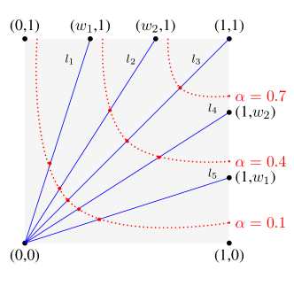
(a)

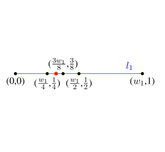
(b)

Figure 2: Graphical representation of the numerical estimation procedure.

Illustration of bivariate level curves on the unit square

We illustrate the bivariate unconditional level curves for known pair copula distributions and the bivariate conditional level curves for a 3-dimensional vine structure. They correspond to the case of no predictors or 1 predictor in a regression setting, respectively. In Figure 3 we explore plots of the unconditional level curves on the unit square for the bivariate Gauss, Student-t, Clayton and Gumbel copulas (rows) with different strengths of dependency, expressed through Kendall’s $\tau$ (Kendall, 1938), with $\tau=0.25,0.5,0.75$ (columns). The level curves can be obtained in an analogous way for any other copula family. The theoretical level curves of a bivariate random vector $\left(V_{1},V_{2}\right)^{T}$ with bivariate distribution function $C_{V_{1},V_{2}}\left(v_{1},v_{2};\theta\right)$ and a parameter $\theta$ are derived using Equation 15 for a given $\alpha$ and are depicted with thick black lines.

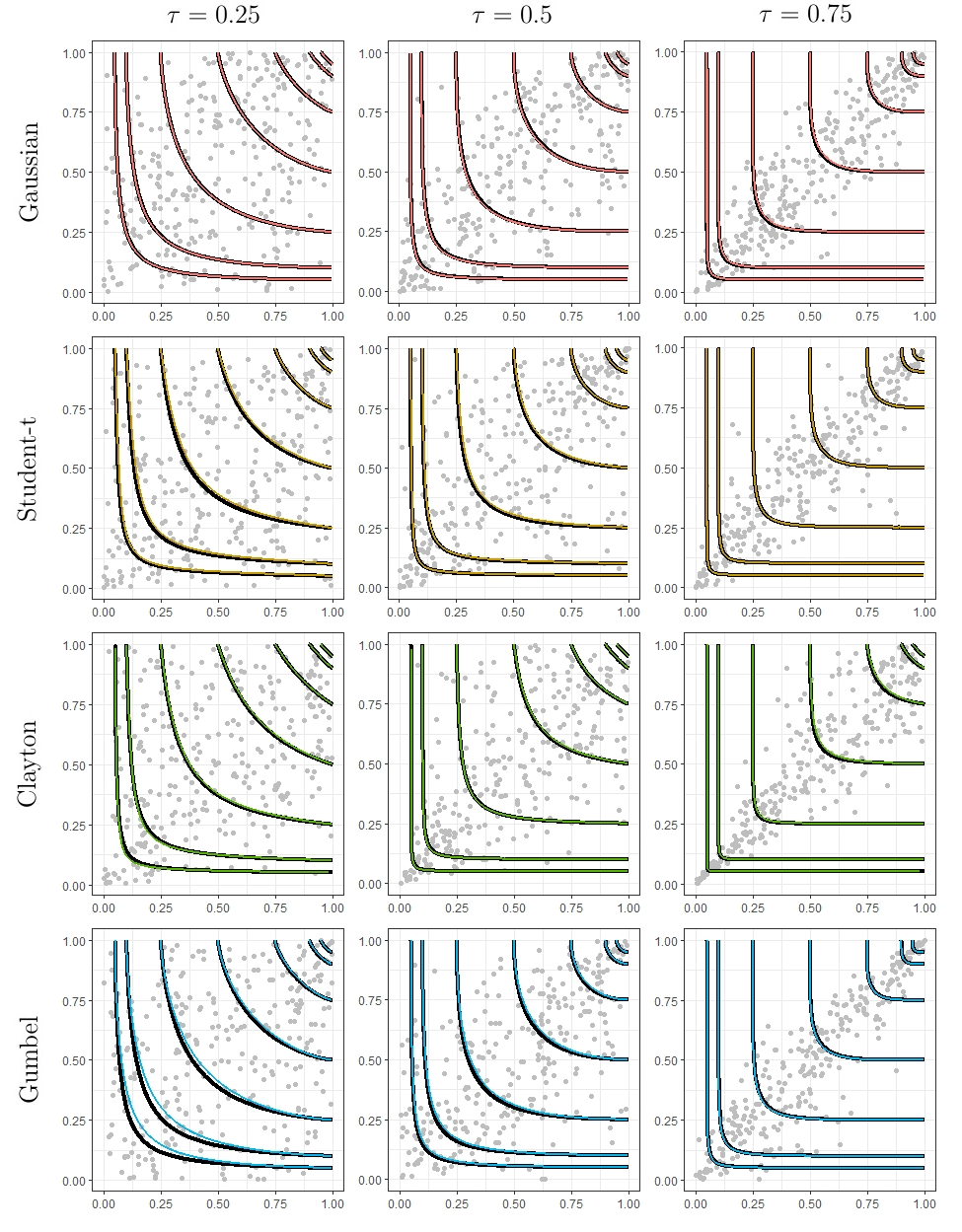
Figure 3: x-axis: $V_{1}$, y-axis: $V_{2}$. Gray points: simulated data from copula (n=300). Black curves: theoretical quantile curves. Colored curves: estimated quantile curves. Depicted are quantile curves for $\alpha=0.05,0.1,0.25,0.5,0.75,0.90,0.95$ (left bottom to right top in each panel) for Gaussian, Student-t ($df=5$), Clayton and Gumbel copulas (top to bottom) and $\tau=0.25,0.5,0.75$ (left to right).

Further, we estimate the bivariate level curves for the given pair copulas. For this we simulate data from the given copula and based on the simulated data, a pair copula is estimated. The gray points are $300$ data points simulated from the given copulas. Subsequently, level curves are evaluated and plotted. The coloured lines represent the corresponding estimated level curves. In the supplementary material we give a detailed description on how the theoretical and the estimated level curves are obtained for each of the four copula families. The panels of Figure 3 showcase bivariate level curves at $\alpha=0.05,0.1,0.25,0.5,0.75,0.90,0.95$.

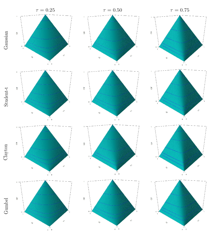
Figure 9: A 3-dimensional plot of bivariate copula distribution with theoretical level curves for $\alpha=0.05,0.1,0.25,0.5,0.75,0.90,0.95$. Shown are Gaussian, Student-t ($df=5$), Clayton and Gumbel copulas (top to bottom) and $\tau=0.25,0.5,0.75$ (left to right).

Differences can be spotted between estimated and theoretical level curves only for the Gumbel level curves, in the case when Kendall’s $\tau=0.25$. In all other cases, differences between the theoretical and estimated level curves are not visible. When it comes to differences in the level curves for different copula families, the Clayton copula level curve has a significantly smaller area below the $\alpha=0.05$ level curve caused by its heavy lower tail (expected realizations are closer to the lower diagonal as compared to a lighter lower tail copula) compared to the other copula families at the $\alpha=0.05$ level curve. On the other hand, the heavy upper tail of the Gumbel copula is causing a bigger area above the $\alpha=0.95$ level curve compared to the Clayton copula. In contrast, the Gaussian copula has no tails at all and the Student-t copula has a symmetric tail dependence governed by a single parameter. Their area below the $\alpha=0.05$ level curve is greater than the corresponding area in the lower heavy-tailed Clayton copula, and the area above the $\alpha=0.95$ level curve is smaller than the upper heavy-tailed Gumbel copula. Considering the $\alpha=0.5$ level curve, the greatest area below it has the Gumbel copula, due to it upper heavy tail, and the smallest area below the $\alpha=0.5$ level curve has the Clayton copula, again due to the heavy lower tail. This holds for all Kendall’s $\tau$ values. Also, as the dependence between the variables increases, the data is more centered around the diagonal, so the curves have sharper curvature around the diagonal. Further, Figure 9 in Appendix C, shows the associated bivariate distribution functions in a 3-dimensional plot in which the theoretical level curves are shown at given $\alpha$ levels.

Next we consider conditional bivariate level curves arising from a 3-dimensional regular vine distribution $\mathcal{D}_{3}$. Let $\left(V_{1},V_{2},U_{1}\right)^{T}\sim\mathcal{D}_{3}$ with vine tree sequence and pair copulas of $\mathcal{D}_{3}$ given by Figure 4.

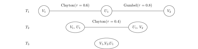
Figure 4: Vine tree sequence of $\mathcal{D}_{3}$ with the pair copula families and Kendall’s $\tau$ corresponding to parameters.

The corresponding parameters of the copulas are $\theta_{V_{1},U_{1}}=3\;(\tau=0.6),\theta_{U_{1},V_{2}}=5\;(\tau=0.8$ )and $\theta_{V_{1},V_{1};U_{1}}=1.33\;(\tau=0.4)$. To obtain theoretical level curves from $\mathcal{D}_{3}$ we employ the following procedure. To evaluate $C_{V_{1},V_{2}|U_{1}}$ at a specific point $\left(\tilde{v}_{1},\tilde{v}_{2}\right)$ conditioned on $U_{1}=\tilde{u}_{1}$ we use Equation 10. The corresponding conditional level curve is evaluated using the numerical evaluation procedure from Section 5.3 and Equation 10. We are also interested in the estimated conditional level curves. To obtain them, we simulate a data set $\mathbf{W}\in\left[0,1\right]^{504\times 3}$ from $\mathcal{D}_{3}$ and split $\mathbf{W}$ into $\mathbf{W}_{train}\in\mathbb{R}^{500\times 3}$ and $\mathbf{W}_{test}\in\mathbb{R}^{4\times 3}$. On the training set $\mathbf{W}_{train}$ we fit a vine model $\hat{\mathcal{D}}_{3}$ with the same vine tree structure and order of the variables as the data generator $\mathcal{D}_{3}$. In 3 dimensions, a C- and a D-vine tree structure coincide, so by order we mean the order from left to right in which the variables appear in the first tree of the sequence, as defined for a general D-vine copula. The estimated pair copulas are $\hat{C}_{V_{1},U_{1}}\sim\;Clayton\left(\hat{\tau}=0.57,\;\hat{\theta}_{V_{1},U_{1}}=2.65\right),$ $\hat{C}_{U_{1},V_{2}}\sim\;Gumbel\left(\hat{\tau}=0.79,\;\hat{\theta}_{U_{1},V_{2}}=4.92\right),$ $\hat{C}_{V_{1},V2;U_{1}}\sim\;Clayton\left(\hat{\tau}=0.40,\;\hat{\theta}_{V_{1},V_{2};U_{1}}=1.34\right).$

The corresponding conditional level curves of $\hat{\mathcal{D}}_{3}$ are obtained using the numerical evaluation procedure from Section 5.3 and evaluating $\hat{C}_{V_{1},V2;U_{1}}$ in a similar manner as in Equation 10, using the estimates of each term.

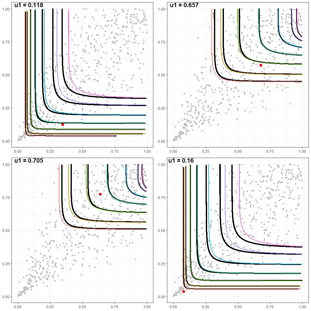
Figure 5: x-axis: $V_{1}$, y-axis: $V_{2}$. Gray points: simulated data from vine distribution (n=500). Black curves: theoretical conditional level curves. Colored curves: estimated conditional level curves. Depicted are level curves at $\alpha=0.05,0.1,0.25,0.5,0.75,0.90,0.95$ (left bottom to right top in each panel). Red dot: associated values of $(v_{1},v_{2})$ with $u_{1}$ as conditioning value.

Note that the estimated and the data-generating vine are approximately very close, due to the use of the same tree structure in both data generation and estimation. But in practice this is not the case, as the underlying tree structure is unknown. However, we can use the Y-vine regression model developed in Section 3 to model the tree structure and the pair copulas, in a way that the joint conditional distribution is easy to be estimated. Figure 5 shows the theoretical and the estimated level curves for 4 conditioning values of $u_{1}$. The values of $u_{1}$ are chosen from $\mathbf{W}_{test}$. The level curves depend on the conditioning value. If the value of $u_{1}$ is low (top-left and bottom-right plot) the level curves are more restricted to the lower left corner. For greater values of $u_{1}$ (top-right and bottom-left plot) the level curves are more restricted to the top right corner. These occurrences can be explained by the high positive dependence of the pairs $(V_{1},U_{1})$ and $(V_{2},U_{1})$ in the first tree of the vine structure, meaning that low values of $u_{1}$ correspond to low values of both $v_{1},v_{2}$. Thus, Figures 3 and 5 show that the numerical procedure for obtaining both unconditional and conditional level curves properly determines the bivariate level curves. We will employ this method to estimate conditional level curves in the case of more than one conditioning value (corresponding to more than one predictor in a regression setting). In the case where we have bivariate regression data available we will fit a Y-vine regression model and use the estimated parameters to determine the associated bivariate level curves.

5.4 Bivariate quantile curves

The notion of multivariate quantiles is not trivial nor well-defined. In the past, the level sets or curves of a multivariate distribution are considered as multivariate quantile, however in this case the coverage probability is not exact. For example, in Fernández-Ponce and Suárez-Lloréns, (2002) the bivariate unconditional quantiles are defined as the level sets of a bivariate distribution function. The authors state that this definition is a natural generalization of the univariate quantile sets (Lewis and Thompson, 1981), however later in Belzunce et al., (2007) it is shown that the level curves do not have the property that the $\alpha$-th level curve separates the lowest $\alpha\times 100$ percent of the observations from the remaining $\left(1-\alpha\right)\times 100$ percent of the observations. Thus, we suggest to define the bivariate quantile curves as adjusted level curves where the coverage probability is exact. Since we are interested in a regression setting, the following study is done on the conditional case, however, the same methodology can be applied for the unconditional case. Also, we define the bivariate quantiles on the u-scale (copula level), and to transform the bivariate quantiles on the x-scale, we use the same analogy as for the level curves. Consider any bivariate vector $\mathbf{q}=\left(q_{1},q_{2}\right)\in Q_{\alpha}^{V}(\mathbf{u})$ that lies on the level curve $Q_{\alpha}^{V}(\mathbf{u})$ for some $\alpha\in(0,1)$. Further, let $S_{\mathbf{q}}$ be a set of bivariate vectors defined by $S_{\mathbf{q}}\coloneqq\{(v_{1},v_{2})\in[0,1]^{2}\;;\;v_{1}\leq q_{1},v_{2}\leq q_{2}\}.$ Then for any random vector $\mathbf{W}=(W_{1},W_{2})^{T}\sim C_{V_{1},V_{2}|\mathbf{U}}(\cdot,\cdot|\mathbf{u})$ it holds that $P\left(\mathbf{W}\in S_{\mathbf{q}}\right)=\alpha,$ by following Equation 16. In Figure 6 we can see an exemplary illustration for the set $S_{\mathbf{q}}$.

Figure 6: A randomly chosen $\mathbf{q}=\left(q_{1},q_{2}\right)$ vector, its corresponding $S_{\mathbf{q}}$ and $S_{\alpha}^{lower},$ where $S_{\alpha}^{lower}=S_{\mathbf{q}}\bigcup A\bigcup B$.

Let the region $S_{\alpha}^{lower}$ be defined as the set of bivariate vectors below the level curve $Q_{\alpha}^{V}(\mathbf{u})$,

$$S_{\alpha}^{lower}\coloneqq\bigcup_{\forall\left(q_{1},q_{2}\right)\in Q_{\alpha}^{V}(\mathbf{u})}\left\{(v_{1},v_{2})\in[0,1]^{2};v_{1}<q_{1},v_{2}<q_{2}\right\}.$$

Then for the random vector $\mathbf{W}=(w_{1},w_{2})^{T}$ it holds that

$$\mathbb{P}\left(\mathbf{W}\in S_{\alpha}^{lower}\right)>\alpha,$$ (17)

since $S_{\mathbf{q}}\subset S_{\alpha}^{lower}$ for all $\mathbf{q}=\left(q_{1},q_{2}\right)\in Q_{\alpha}^{V}(\mathbf{u}),$ as also noted in Fernández-Ponce and Suárez-Lloréns, (2002). (See Figure 6 to observe the $S_{\alpha}^{lower}$ region.) This implies that the level curve $Q_{\alpha}^{V}(\mathbf{u})$ divides the $\left[0,1\right]^{2}$ square into a region for which it holds that $\mathbb{P}\left(\mathbf{W}\in S_{\alpha}^{lower}\right)\neq\alpha.$ It also follows that $\mathbb{P}\left(\mathbf{W}\notin S_{\alpha}^{lower}\right)<1-\alpha.$ Thus, for the definition of a $\alpha$ quantile curve we want to find an adjusted $\beta(\alpha)$ level curve which will divide the observation space into $\alpha$ and $1-\alpha$ percent, i.e. for which $\mathbb{P}\left(\mathbf{W}\in S_{\beta(\alpha)}^{lower}\right)=\alpha$ holds.

Definition .

The bivariate conditional quantile for $\alpha\in\left(0,1\right)$, a transformation $\beta:(0,1)\longmapsto(0,1)$ and continuous random variables $Y_{1},Y_{2}$ with random PITs $V_{1},V_{2}$ given the outcome of the random vector $\mathbf{X}=\mathbf{x},$ with PITs $\mathbf{U}=\mathbf{u}$ is a curve in $[0,1]^{2}$ defined by the set

$$q_{\alpha}^{V}(\mathbf{u})\coloneqq\{(v_{1},v_{2})\in[0,1]^{2}\;;\;C_{V_{1},V_{2}|\mathbf{U}}(v_{1},v_{2}|\mathbf{u})=\beta(\alpha)\},$$ (18)

so that the observation space is divided into $\alpha$ and $1-\alpha$ percent regions, i.e. $\mathbb{P}\left(\mathbf{W}\in S_{\beta(\alpha)}^{lower}\right)=\alpha$ holds.

Following Definition 5.4, we can also define an exact $100\times\left(1-\alpha\right)\%$ confidence region arising from the quantile curves $q_{\alpha/2}^{V}(\mathbf{u})$ and $q_{1-\alpha/2}^{V}(\mathbf{u})$.

Definition .

The $100\times\left(1-\alpha\right)\%$ bivariate confidence region for $\alpha\in\left(0,1\right)$ and a continuous bivariate vector continuous random variables $Y_{1},Y_{2}$ with random PITs $V_{1},V_{2}$ given the outcome of the random vector $\mathbf{X}=\mathbf{x},$ with PITs $\mathbf{U}=\mathbf{u}$, is set of points in $[0,1]^{2}$ enclosed by the quantile curves $q^{V}_{\alpha/2}\left(\mathbf{u}\right)$ and $q^{V}_{1-\alpha/2}\left(\mathbf{u}\right)$, i.e.

$$CI^{V_{1},V_{2}|\mathbf{U}}_{\alpha}\coloneqq\bigg{\{}\left(w_{1}^{*},w_{2}^{*}\right)\in[0,1]^{2}\;\big{|}\;\exists\;\left(v^{1}_{1},v^{1}_{2}\right)\in q^{V}_{\alpha/2}\left(\mathbf{u}\right), \;\left(v^{2}_{1},v^{2}_{2}\right)\in q^{V}_{1-\alpha/2}\left(\mathbf{u}\right)\;such\;that:$$

$$\;\;v^{1}_{1}\leq w_{1}^{*}\leq v^{2}_{1}\;\;and\;\;v^{1}_{2}\leq w_{2}^{*}\leq v^{2}_{2}\bigg{\}}.$$

In this case, $\mathbb{P}(\mathbf{W}\in CI^{V_{1},V_{2}|\mathbf{U}}_{\alpha})=\mathbb{P}(\mathbf{W}\in S_{\beta(\alpha/2)}^{lower})-\mathbb{P}(\mathbf{W}\in S_{\beta(1-\alpha/2)}^{lower})=\alpha/2-(1-\alpha/2)=1-\alpha,$ implying that $CI^{V_{1},V_{2}|\mathbf{U}}_{\alpha}$ is an exact $100\times\left(1-\alpha\right)\%$ confidence region. Returning back to the problem of estimating the transformation $\beta(\alpha)$, for $\beta:(0,1)\longmapsto(0,1)$, so that the quantile curves $q_{\alpha}^{V}(\mathbf{u})$ are estimated, we suggest a numerical procedure. Basically, we need to change the $\alpha$-level curve to a new $\beta(\alpha)$- level curve so that $\mathbb{P}(\mathbf{W}\in S_{\beta(\alpha)}^{lower})=\alpha$ holds true. To achieve this, we define the function

$$G(\beta) \coloneq\mathbb{P}\left(\mathbf{W}\in S_{\beta}^{lower}\right)$$ (19)

$$=\mathbb{P}\left(C_{V_{1},V_{2}|\mathbf{U}}(\cdot,\cdot|\mathbf{u})\leq\beta\right)\;\;\forall\;\beta\in(0,1).$$

From Equation 17 we can see that $G(\alpha)>\alpha$. However, we are interested to find the value $\beta(\alpha)$ so that it holds that $G(\beta(\alpha))=\alpha$, thus $\beta(\alpha)=G^{-1}(\alpha).$ To do so, we suggest a numerical procedure. As the function $G(\beta)$ is difficult to evaluate analytically, we suggest to estimate it using a simulated sample from the Y-vine copula with $\mathbf{U}=\mathbf{u}$ fixed. For $n=1,\cdots,N$ we simulate observations $\left(v_{1}^{n}(\mathbf{u}),v_{2}^{n}(\mathbf{u})\right)\sim C_{V_{1},V_{2}|\mathbf{U}}\left(\cdot,\cdot|\mathbf{u}\right)$, as described in Section 4.1. Then, we estimate $G(\beta)$ as the proportion of the simulated data below the $\alpha$-quantile over the sample size N, i.e.

$$\hat{G}\left(\beta\right)=\frac{1}{N}\sum_{n=1}^{N}\mathbb{I}\left(\left(v_{1}^{n}(\mathbf{u}),v_{2}^{n}(\mathbf{u})\right)\in S_{\beta}^{lower}\right),$$

where $\mathbb{I}$ is an indicator function, being equal to 1 when the condition $\left(v_{1}^{n}(\mathbf{u}),v_{2}^{n}(\mathbf{u})\right)\in S_{\beta}^{lower}$ is satisfied, and equal to 0, otherwise. To find the desired $\beta(\alpha)$ we use a line search algorithm on the $(0,1)$ interval and obtain the estimated $\hat{\beta}(\alpha)$ such that $\hat{G}(\hat{\beta}(\alpha))=\alpha$. This way the suggested methodology from Section 5 can be extended to find the bivariate quantiles $q_{\alpha}^{V}(\mathbf{u})$ such that $\hat{G}(\beta(\alpha))=\mathbb{P}\left(\mathbf{W}\in S_{\beta(\alpha)}^{lower}\right)=\alpha,$ holds, i.e. the $\beta(\alpha)$-th level set separates the lowest $\alpha\times 100$ percent of the observations from the remaining $\left(1-\alpha\right)\times 100$ percent of the observations.

Another concept for the construction of exact confidence regions is been developed in Coblenz et al., (2018). The authors propose, to construct an exact confidence region for unconditional bivariate copula distribution functions. They use the Kendall distribution function of a bivariate copula $C$ at a level $\alpha\in(0,1)$, $K(C,\alpha)$ defined as $K(C,\alpha)\coloneqq\mathbb{P}\left(C(U,V)\leq\alpha,\;(U,V)\sim C\right),$ in Genest and Rivest, (1993) and Barbe et al., (1996). In comparison to our methodology it holds that $G(\beta(\alpha))=K(C,\alpha)$ in the unconditional case, as shown in Chakak and Ezzerg, (2000). For bivariate copula distribution functions computing the Kendall distribution function is possible and certain approaches are available (Chakak and Ezzerg, 2000; Ezzerg et al., 1999), however it is very computationally expensive (Brechmann, 2013). Once $K$ is estimated, $\beta(\alpha)$ can be obtained as the inverse of the Kendall distribution function evaluated at $\alpha$, i.e. $\beta(\alpha)=K^{-1}(C,\alpha)$. Estimating the Kendall distribution functions in the conditional case is difficult in general and computationally expensive, however the same results are expected to follow as for the unconditional case.

6 Data application

The implementation of the Y-vine quantile regression is done in the statistical software R (R Core Team, 2021). As an application to real data we consider the Seoul weather data set, which contains two dependent responses, daily minimum and maximum air temperature. The data originates from the UCI machine learning repository (Dua and Graff, 2019), it can be downloaded using https://archive.ics.uci.edu/ml/ datasets/Bias+correction+of+numerical+prediction+model+temperature+forecast and was first studied by Cho et al., (2020). It contains daily data for 25 weather stations in Seoul, South Korea between June 30th and August 30th in the period 2013-2017. Cho et al., (2020) use it for enhancing next-day maximum and minimum air temperature forecasts based on the Local Data Assimilation and Prediction System (LDAPS) model. To illustrate the proposed vine based bivariate quantile regression model, we consider the station located in central Seoul (station 25) and and we model the temporal dependence in the responses, by considering the present minimum and maximum air temperature (including two lagged variables into the regression model) when modeling next day values. Disregarding geographical markers and precipitation measurements, we are left with a data set containing two response variables and 13 continuous predictors, with 307 data points representing summer days of the years 2013 to 2017. In the supplementary material we provide a description of the considered variables. We divide the data set into a training and testing set, consisting of 246 data points from 2013-2016, and 61 data points from 2017, respectively. In the supplement, we also show the empirical normalized contour plots for pairs of variables from the training set, which shows strong non-Gaussian dependence structure in the data, indicated by non-elliptical shapes. This shows that the data is suited for application of the proposed Y-vine copula class. In the estimation of our Y-vine quantile regression model we model the marginals distributions using a nonparametric approach, while we model the pair copulas in a parametric approach, resulting in a semiparametric model. Modeling the marginals as well as the copulas parametrically might cause the resulting fully parametric estimator to be biased and inconsistent if one of the parametric models is misspecified Noh et al., (2013). Modeling them both using a nonparametric approach leads to a fully nonparametric approach that might overfit the data, because penalization is still an open research topic in the nonparametric case, as noted in Tepegjozova et al., (2022). Thus, we opt for a semiparametric approach. The marginals are estimated using a univariate nonparametric kernel density estimator implemented in the R package kde1d (Nagler and Vatter, 2020), and the pair copulas are fitted using a parametric maximum-likelihood approach with the Akaike Information Criterion penalization (Akaike, 1973) (AIC) implemented in the R package rvinecopulib (Nagler and Vatter, 2021). Further, we use as selection criteria for the forward selection of predictors the AIC penalized $acll,$ (defined in 11) in order to favour a more sparse model.

The automatically chosen order of the predictors in the fitted Y-vine regression model $\hat{{\mathcal{Y}}}$ is given by

$$\begin{split}O(\hat{{\mathcal{Y}}})=&\left(\texttt{ LDAPS\_Tmin\_lapse, LDAPS\_Tmax\_lapse, LDAPS\_CC1, LDAPS\_WS, }\right.\\ &\left.\texttt{ Present\_Tmin, LDAPS\_RHmax, LDAPS\_CC3, LDAPS\_LH, Present\_Tmax}\right).\end{split}$$

It orders the predictors by their influence over the two responses. Also, only 9 out of 13 possible predictors are chosen to be in the model. The 4 non-influential predictors, based on the Y-vine model are LDAPS_CC2, LDAPS_CC4, LDAPS_RHmax and solar radiation. More details on the fitted pair copulas selected by the Y-vine regression model is given in the supplement, in Tables 2 and 3. The fitted pair copula between the responses given the 9 chosen predictors, $\hat{c}_{V_{1},V_{2};\mathbf{U}}$ is a Joe copula with an estimated Kendall’s $\tau$ of 0.09. This implies that after the effect of the predictors is adjusted in the model, there is little dependence between the responses. For illustrating the unconditional level curves of the joint unconditional bivariate distribution of the two responses, U_max and U_min we fit a pair copula between them. The estimated pair copula is the Gaussian copula with a parameter of 0.66. The unconditional quantile curves are defined as in Definition 5.4 by using the pair copula distribution function between the responses $C_{V_{1},V_{2}}$, instead of the bivariate conditional distribution $C_{V_{1},V_{2}|\mathbf{U}},$ and we denote them as $q_{\alpha}^{V}$ for $\alpha\in(0,1)$. The level curves of this copula, on both the x- and the u-scale are given in Figure 7. Note that the maximum temperature is always greater than the minimum temperature. However, this ordering constraint does not imply an ordering constraint on the PITs on the u-scale (as the marginal distributions are separately and independently modeled). For illustration see Figure 7, where the ordering is visible in panel $(a)$, as all the data is below the diagonal, while this ordering is lost in panel $(b).$

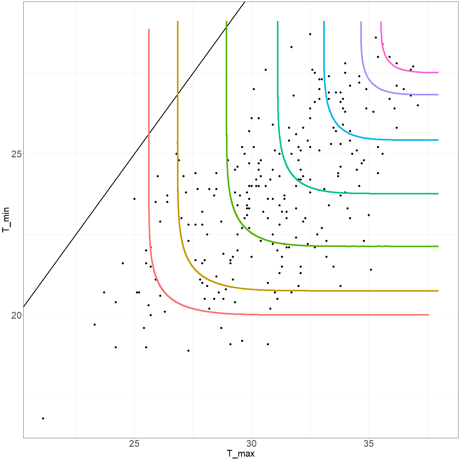
(a) $x$-scale

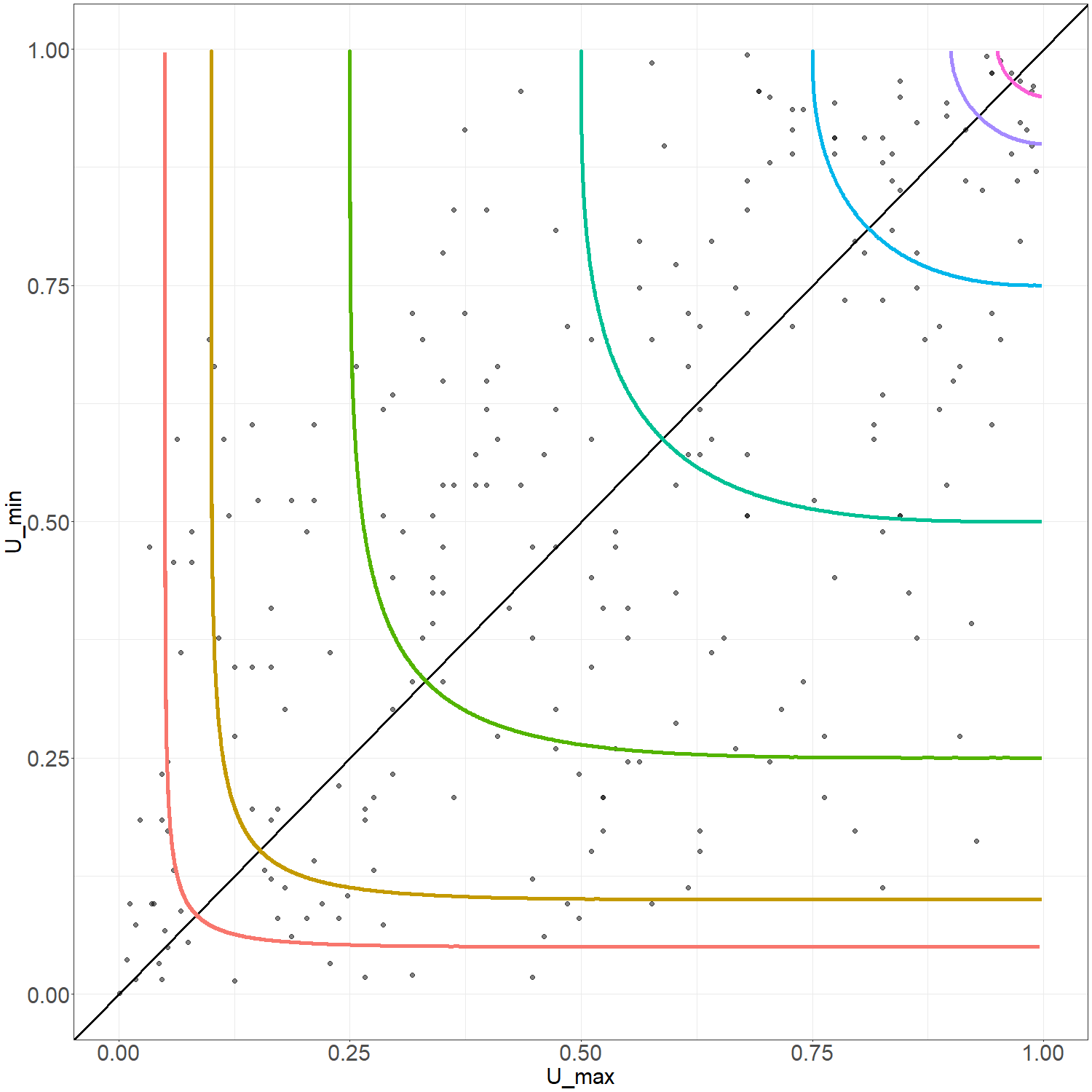
(b) $u$-scale

Figure 7: Black points: data from 2013-2016 (n=246). Colored curves: estimated unconditional level curves at $\alpha=0.05,0.1,0.25,0.5,0.75,0.90,0.95$ (left bottom to right top).

6.1 Bivariate quantile curves, confidence regions and advantages of joint modeling of dependent responses

For comparison purposes we consider 4 different scenarios: 1.) $U_{max}$ and $U_{min}$ are jointly modeled using a bivariate copula, 2.) $U_{max}$ and $U_{min}$ are independent, 3.) $U_{max}$ and $U_{min}$ are conditional independent given the predictors and 4.) $U_{max}$ and $U_{min}$ are jointly modeled with the predictors. The first 2 cases are the unconditional cases, and the last 2 are the conditional case. For 1.) consider the unconditional quantile curves and the corresponding confidence region obtained from fitting a bivariate copula between the responses $U_{max}$ and $U_{min}$, and the confidence region obtained by assuming dependence between the responses. The unconditional quantile curves are defined as in Definition 5.4 by using the pair copula between the responses $C_{V_{1},V_{2}}$, instead of the bivariate conditional distribution $C_{V_{1},V_{2}|\mathbf{U}},$ and are denoted as $q_{\alpha}^{V}$ for $\alpha\in(0,1)$. Using Definition 5.4, by substituting the conditional quantile curves with the unconditional ones, we can define the corresponding unconditional confidence region $CI^{V_{1},V_{2}}_{\alpha}$ as set of points in $[0,1]^{2}$ enclosed by the quantile curves $q^{V}_{\alpha/2}$ and $q^{V}_{1-\alpha/2}$ for some $\alpha\in(0,1)$, i.e.

$$CI^{V_{1},V_{2}}_{\alpha}\coloneqq\bigg{\{}\left(w_{1}^{*},w_{2}^{*}\right)\in[0,1]^{2}\;\big{|}\;\exists\;\left(v^{1}_{1},v^{1}_{2}\right)\in q^{V}_{\alpha/2}, \;\left(v^{2}_{1},v^{2}_{2}\right)\in q^{V}_{1-\alpha/2}\;such\;that:$$

$$\;\;v^{1}_{1}\leq w_{1}^{*}\leq v^{2}_{1}\;\;and\;\;v^{1}_{2}\leq w_{2}^{*}\leq v^{2}_{2}\bigg{\}}.$$

For 2.) we construct a bivariate quantile region from the univariate empirical quantiles, denoted as $q_{\alpha,emp}^{V_{1}}$ for $\alpha\in(0,1),$ using the Bonferroni correction for multiple testing (Bonferroni, 1936). We are interested in the bivariate quantile region with coverage probability at $\alpha\in(0,1)$ meaning that the two univariate empirical quantiles, from which we construct the bivariate quantile region, need to be evaluated at $\frac{\alpha}{4}$ and $1-\frac{\alpha}{4}$, and we denote the corresponding confidence region of the univariate empirical quantiles as $CI^{V_{1}\perp V_{2}}_{\alpha}$, i.e.

$$CI^{V_{1}\perp V_{2}}_{\alpha}\coloneq\left[q_{\frac{\alpha}{4},emp}^{V_{1}},q_{1-\frac{\alpha}{4},emp}^{V_{1}}\right]\times\left[q_{\frac{\alpha}{4},emp}^{V_{2}},q_{1-\frac{\alpha}{4},emp}^{V_{2}}\right].$$

For 3.) we treat the response variables as conditionally independent given a set of predictors. Basically, the tasks of predicting maximal and minimal temperatures given the predictors are treated as completely independent problems and univariate conditional quantiles are estimated for both response variables. For this purpose, two univariate $D$-vine regression models with the same predictor order as the Y-vine regression are fitted. The D-vine is a natural subset model of the Y-vine tree sequence when considering a single response variable. This way we can construct a bivariate quantile region from the univariate quantiles using the Bonferroni correction for multiple testing (Bonferroni, 1936), similar as before for the unconditional case. We denote these univariate D-vine based quantiles as, $q_{\alpha,Dvine}^{V}(\mathbf{u})$ for $\alpha\in(0,1).$ We are interested in the bivariate quantile region with coverage probability of $\alpha$ meaning that the two univariate quantiles, need to be evaluated at $\frac{\alpha}{4}$ and $1-\frac{\alpha}{4}$, and we denote the corresponding confidence region using the univariate conditional quantiles as $CI^{V_{1}\perp V_{2}|\mathbf{U}}_{\alpha}$, i.e.

$$CI^{V_{1}\perp V_{2}|\mathbf{U}}_{\alpha}\coloneq\left[q_{\frac{\alpha}{4},Dvine}^{V_{1}}(\mathbf{u}),q_{1-\frac{\alpha}{4},Dvine}^{V_{1}}(\mathbf{u})\right]\times\left[q_{\frac{\alpha}{4},Dvine}^{V_{2}}(\mathbf{u}),q_{1-\frac{\alpha}{4},Dvine}^{V_{2}}(\mathbf{u})\right].$$

For case 4.) we use the fitted Y-vine copula as discussed in Sections 5.2 and 5.4. The first row of Figure 8, shows the bivariate level curves (solid lines) and quantile curves (dashed lines), where the first column is the unconditional case (case 1.) and 2.)), while second and third columns are conditional cases for two randomly chosen dates 02.07 and 21.08 (case 3.) and 4.)), respectively. The adjusted level curves, the bivariate quantiles are estimated using the proposed method introduced in Section 5.4. From the fitted pair copula (or vine copula), we simulate 10 000 data points from which the quantile curves are estimated and the simulated points are shown as well. For all $\alpha$ levels, the estimated empirical coverage probabilities $\hat{G}(\alpha)$ are evaluated so that we can estimate the adjustment $\hat{\beta}(\alpha)$ for the corresponding quantile levels.

For the unconditional case, the estimated values for the adjustment to quantile curves (dashed lines) are $\hat{\beta}(0.25)=0.14,$ $\hat{\beta}(0.75)=0.59$ and $\hat{\beta}(0.05)=0.02,$ $\hat{\beta}(0.95)=0.86$. Using these values, we construct the confidence regions $CI_{0.50}^{V_{1},V_{2}}$ and $CI_{0.90}^{V_{1},V_{2}}$, respectively. The second row, first column shows the $CI^{V_{1},V_{2}}_{0.50}$ (green region, case 1.)) and $CI^{V_{1}\perp V_{2}}_{0.50}$ (gray region, case 2.) ). Last row, first column shows the $CI^{V_{1},V_{2}}_{0.90}$ (red region, case 1.)) and $CI^{V_{1}\perp V_{2}}_{0.90}$ (gray region, case 2.)). The estimated empirical coverage probabilities and the adjusted levels for each case are given in the supplement in Table 4. The empirical coverage probability, based on the 10 000 samples, for the $CI_{0.50}^{V_{1},V_{2}}$ is 0.50, while the coverage probability below the level curve at $\alpha=0.25$ is 0.41, and below the level curve at $\alpha=0.75$ is 0.89. However, the empirical coverage probability for $CI_{0.50}^{V_{1}\perp V_{2}}$ is 0.65, thus we see the effect of falsely assuming independence between $V_{1}$ and $V_{2}$. The empirical coverage probability for $CI_{0.90}^{V_{1},V_{2}}$ is 0.90, while the coverage probability below the level curve at $\alpha=0.05$ is 0.10, below the level curve at $\alpha=0.95$ is 0.99. However, the empirical coverage probability for $CI_{0.90}^{V_{1}\perp V_{2}}$ is 0.91.

For the conditional case, the estimated values for the adjustment to quantile curves (dashed lines) are given in the supplement in Tables 5 and 6. For the date 02.07.2017, the estimated values for the adjustment to quantile curves (dashed lines) are $\hat{\beta}(0.25)=0.11,$ $\hat{\beta}(0.75)=0.48$ and $\hat{\beta}(0.05)=0.03,$ $\hat{\beta}(0.95)=0.85$. The empirical coverage probability below the level curve at $\alpha=0.25$ is 0.52, below the level curve at $\alpha=0.75$ is 0.91 and below $\alpha=0.05$ is 0.12, below $\alpha=0.95$ is 0.99. For 21.08.2017, the estimated values for the adjustment to quantile curves (dashed lines) are $\beta(0.25)=0.16,$ $\beta(0.75)=0.66$ and $\hat{\beta}(0.05)=0.025,$ $\hat{\beta}(0.95)=0.91.$ The empirical coverage probability below the level curve at $\alpha=0.25$ is 0.37, below the $\alpha=0.75$ is 0.83, below $\alpha=0.05$ is 0.10 and below the level curve at $\alpha=0.95$ is 0.98. The second row shows $CI_{0.50}^{V_{1},V_{2}|\mathbf{U}}$ (green, case 4.) ) and $CI_{0.50}^{V_{1}\perp V_{2}|\mathbf{U}}$ (gray, case 3.)), while the third row shows $CI_{0.90}^{V_{1},V_{2}|\mathbf{U}}$ (red, case 4.)) and $CI_{0.90}^{V_{1}\perp V_{2}|\mathbf{U}}$ (gray, case 3.)) for two different conditioning values for dates 02.07 and 21.08. While the confidence regions $CI_{0.50}^{V_{1},V_{2}|\mathbf{U}}$ have exact empirical coverage probabilities, for 02.07 the coverage probability of $CI_{0.50}^{V_{1}\perp V_{2}|\mathbf{U}}$ is 0.17, and for 21.08 it is 0.25. Similarly, $CI_{0.90}^{V_{1},V_{2}|\mathbf{U}}$ have exact empirical coverage probabilities, but for 02.07 the empirical coverage probability of $CI_{0.90}^{V_{1}\perp V_{2}|\mathbf{U}}$ is 0.59, and for 21.08 it is 0.66. Thus, for the unconditional case, in case 2.) the empirical coverage probabilities are close to the expected value, but for the conditional case 3.) where we assume conditional independence the empirical coverage probabilities are much smaller than their expected value. Thus, in this case the empirical coverage probability is underestimated, leading to underestimation of the areas of interest, while in case 1.) and 4 .) the coverage probabilities are equal to the expected level. In Figure 8, all the panels are given on the u-scale. However, using the transformations of the level curves between the u-scale and the x-scale, explained in Section 5.1, we also provide all the level curves, quantile curves and the corresponding confidence regions on the transformed x-scale in the supplement in Figure 2.

There is obvious difference in the obtained shapes of confidence regions arising from bivariate quantiles (dependent responses) and the univariate quantiles based regions (conditionally independent responses). While the bivariate confidence regions are areas determined by two level curves, the regions obtained by the univariate confidence intervals are bound to be rectangles. Also, for 21.08.2017 the univariate quantiles based confidence regions are partially contained in the bivariate confidence regions obtained from the Y-vine regression and are of much smaller empirical coverage probabilities. So, there is many points that are excluded from the confidence region constructed from the univariate quantiles. For 02.07.2017, there is a very small overlap between $CI^{V_{1}\perp V_{2}|\mathbf{U}}_{0.50}$ and the bivariate confidence regions obtained from the Y-vine regression $CI_{0.50}^{V_{1},V_{2}|\mathbf{U}}$, while the $CI^{V_{1}\perp V_{2}|\mathbf{U}}_{0.90}$ is a partially contained in the bivariate $CI_{0.90}^{V_{1},V_{2}|\mathbf{U}}$. However, the empirical coverage probabilities are underestimated. All in all, the univariate conditional quantiles based confidence regions have not exact empirical coverage probabilities, are too small in area and don’t capture any joint conditional dependence between the responses. However, the bivariate confidence regions we suggest have the expected empirical coverage probabilities and allow for the dependence and the multidimensional nature of the problem. This example shows that even a small conditional dependence (estimated Kendall’s $\hat{\tau}$ of $C_{V_{1},V_{2}|\mathbf{U}}=0.09$) can make confidence regions based on conditional independence invalid (case 3.)).

Figure 8: First row: level curves (solid lines) and corresponding quantile curves (dashed lines) at $\alpha=0.05,0.1,0.25,0.5,0.75,0.90,0.95$. Second row: first column $CI^{V_{1},V_{2}}_{0.50}$ (green region, case 1.) ) and $CI^{V_{1}\perp V_{2}}_{0.50}$ (gray region, , case 2.)), second and third column $CI^{V_{1},V_{2}|\mathbf{U}}_{0.50}$ (green region, case 4.)) and $CI^{V_{1}\perp V_{2}|\mathbf{U}}_{0.50}$ (gray region, case 3.)). Third row: first column $CI^{V_{1},V_{2}}_{0.90}$ (red region) and $CI^{V_{1}\perp V_{2}}_{0.90}$ (gray region), second and third column $CI^{V_{1},V_{2}|\mathbf{U}}_{0.90}$ (red region) and $CI^{V_{1}\perp V_{2}|\mathbf{U}}_{0.90}$ (gray region). . The blue triangle is the true observed value.

7 Conclusions and outlook

We studied the problem of bivariate (unconditional and conditional) quantiles using a flexible class of models, vine copulas, allowing for asymmetric tail dependence. They are multivariate distributions constructed from bivariate blocks (pair copulas) using conditioning. We develop a novel vine tree structure, the Y-vine tree structure, that is suitable for a regression problem containing bivariate response variables. Also, a forward selection of predictors procedure gives the best suitable fitted Y-vine. In addition, the Y-vine tree structure enables an easy way of obtaining the bivariate conditional density. We propose a numerical procedure for the determination of the level curves of a bivariate (conditional) distribution, and propose a simulation based adjustment of the level $\alpha$ of the level curve resulting in quantile curve with correct probability coverage. This way a joint analysis of the dependence structure of the responses given the predictors is possible. This is a significant result especially when dealing with responses that are not (conditionally) independent. We develop a prediction method for bivariate responses given the predictor values using the Y-vine quantile regression. This enables us to not only jointly model, but also predict bivariate response conditional quantiles. Additionally, simulation from a Y-vine model for fixed predictor values is available. We apply our proposed model on a real life data set containing a bivariate response, minimal and maximal daily temperature. We analyse the data with our new approach for dependent responses and provide a joint vine copula model for the two responses. For this example, we highlight the advantages of our joint bivariate modelling over independent and conditionally independent response modelling approaches with vine copulas.

For future possible applications we think of adding a spatial and/or temporal component to our Y-vine based quantile regression. It would be interesting to see how the response dependence changes when the spatial and/or temporal dependence component is also accounted for, but that is out of the scope of this paper. The standard lack of ability of copula based models to include discrete variables is also an ongoing research topic. Some results from the univariate vine based quantile regression are available (Schallhorn et al., 2017), but it becomes even more complicated in our case, because of the multidimensionality of the problem and the numerical method for obtaining the bivariate quantile sets. Also, applications of different vine structures and variable selection methods, and subsequent comparisons of the performance, are left for further investigation and are expected to be heavily data specific problems. In addition, we can use the Y-vine tree structure for testing of conditional independence between two variables given a set of conditioning variables. The Y-vines provide a symmetric treatment of the two variables whose conditional independence is being tested. Using this way of testing for conditional independence we do not need joint normality nor rely on asymptotic normality results. A similar approach was proposed in Bauer and Czado, (2016) using R-vines, for non-Gaussian conditional independence testing in continuous Bayesian networks. However, their approach needed, possibly high dimensional, integration for determining the required conditional distribution function and thus, is not applicable for large network problems. In contrast, we expect our approach to remain tractable in large networks.

Appendix

Appendix A Appendix A: Algorithms for numerical estimation

Input: m - granularity parameter (default = 1000),

            eq - function based on which $C\left(u,v\right)$ is to be evaluated,

            $err$ - accuracy of algorithm,

            $\alpha$ - alpha level

Initialization:

$$M=\bigcup_{i=1}^{m}\left\{\frac{i}{m}\right\},$$

$$L=\left\{line\left(\left(0,0\right),\left(q_{1},q_{2}\right)\right)\right\},\;\;\left(q_{1},q_{2}\right)\in\left\{\left(w_{i},1\right)|\forall w_{i}\in M\right\}\cup\left\{\left(1,w_{i}\right)|\forall w_{i}\in M\right\},$$

$$Points=\emptyset.$$

for $l_{s}\in L$ do

       if  $C\left(q_{1},q_{2}\right)\geq\alpha$  then

            

$$point=\textrm{BinaryLineSearch}\left(l_{s},\mathbf{eq},err,\alpha\right)$$

$$Points=Points\cup point$$

      else

            

$$Points=Points$$

       end if

      

end for

return $Points$

Algorithm 1 PseudoInverse

Input: l - line defined by two coordinates,

            eq - function based on which $C\left(u,v\right)$ is to be evaluated,

            $err$ - accuracy of algorithm,

            $\alpha$ - alpha level

Initialization:

Introduce notation $\mathbf{l}=line\left(p_{start}=\left(0,0\right),p_{end}=\left(w_{i},1\right)\right)$.

$$evl=\mathbf{eq}\left(\frac{p_{start}+p_{end}}{2}\right)$$

$$diff=\alpha-evl$$

while $diff>err$ do

       if $diff>0$ then

            $p_{start}=\frac{p_{start}+p_{end}}{2}$

      else

            $p_{end}=\frac{p_{start}+p_{end}}{2}$

       end if

      $evl=\mathbf{eq}\left(\frac{p_{start}+p_{end}}{2}\right)$

end while

return $\frac{p_{start}+p_{end}}{2}$

Algorithm 2 BinaryLineSearch

Appendix B Appendix B: Proofs

B.1 Proof of Proposition 3.1

Proof.

$$F_{Y_{1},Y_{2}|\mathbf{X}}\left(y_{1},y_{2}|\mathbf{x}\right) =\int_{-\infty}^{y_{1}}\int_{-\infty}^{y_{2}}f_{Y_{1},Y_{2}|\mathbf{X}}\left(y_{1}^{\prime},y_{2}^{\prime}|\mathbf{x}\right)dy_{2}^{\prime}\;dy_{1}^{\prime}$$

$$=\int_{-\infty}^{y_{1}}\int_{-\infty}^{y_{2}}\frac{f_{Y_{1},Y_{2},\mathbf{X}}\left(y_{1}^{\prime},y_{2}^{\prime},\mathbf{x}\right)}{f_{\mathbf{X}}\left(\mathbf{x}\right)}dy_{2}^{\prime}\;dy_{1}^{\prime}$$

$$=\frac{1}{f_{\mathbf{X}}\left(\mathbf{x}\right)}\int_{-\infty}^{y_{1}}\int_{-\infty}^{y_{2}}\frac{\partial^{p+2}}{\partial y_{1}\;\partial y_{2}\;\partial x_{1}\ldots\partial x_{p}}F_{Y_{1},Y_{2},\mathbf{X}}\left(y_{1},y_{2},\mathbf{x}\right)\Big{|}_{y_{1}=y_{1}^{\prime},y_{2}=y_{2}^{\prime}}dy_{2}^{\prime}\;dy_{1}^{\prime}$$

$$=\frac{1}{f_{\mathbf{X}}\left(\mathbf{x}\right)}\cdot\frac{\partial^{p}}{\partial x_{1}\ldots\partial x_{p}}F_{Y_{1},Y_{2},\mathbf{X}}\left(y_{1},y_{2},\mathbf{x}\right)$$

$$(by\;Sklar^{\prime}s\;theorem) =\frac{1}{f_{\mathbf{X}}\left(\mathbf{x}\right)}\cdot\frac{\partial^{p}}{\partial x_{1}\ldots\partial x_{p}}C_{V_{1},V_{2},\mathbf{U}}\left(F_{Y_{1}}(y_{1}),F_{Y_{2}}(y_{2}),F_{X_{1}}(x_{1}),\ldots,F_{X_{p}}(x_{p})\right)$$

$$=\frac{1}{f_{\mathbf{X}}\left(\mathbf{x}\right)}\cdot\frac{\partial^{p}}{\partial u_{1}\ldots\partial u_{p}}C_{V_{1},V_{2},\mathbf{U}}\left(v_{1},v_{2},u_{1},\ldots,u_{p}\right)\Big{|}_{v_{j}=F_{Y_{j}}(y_{j}),u_{i}=F_{X_{i}}(x_{i})}\frac{\partial u_{1}\ldots\partial u_{p}}{\partial x_{1}\ldots\partial x_{p}}$$

$$\left(\frac{\partial u_{1}\ldots\partial u_{p}}{\partial x_{1}\ldots\partial x_{p}}=\prod_{i=1}^{p}f_{X_{i}}\left(x_{i}\right)\right) =\frac{\partial^{p}}{\partial u_{1}\ldots\partial u_{p}}C_{V_{1},V_{2},\mathbf{U}}\left(v_{1},v_{2},u_{1},\ldots,u_{p}\right)\Big{|}_{v_{j}=F_{Y_{j}}(y_{j}),u_{i}=F_{X_{i}}(x_{i})}\cdot\frac{\prod_{i=1}^{p}f_{X_{i}}\left(x_{i}\right)}{f_{\mathbf{X}}\left(\mathbf{x}\right)}$$

$$\left(\frac{\partial u_{1}\ldots\partial u_{p}}{\partial x_{1}\ldots\partial x_{p}}=\prod_{i=1}^{p}f_{X_{i}}\left(x_{i}\right)\right) =\frac{\partial^{p}}{\partial u_{1}\ldots\partial u_{p}}C_{V_{1},V_{2},\mathbf{U}}\left(v_{1},v_{2},u_{1},\ldots,u_{p}\right)\Big{|}_{v_{j}=F_{Y_{j}}(y_{j}),u_{i}=F_{X_{i}}(x_{i})}\cdot\frac{1}{c_{\mathbf{U}}\left(\mathbf{u}\right)}$$

$$=C_{V_{1},V_{2}|\mathbf{U}}\left(F_{Y_{1}}(y_{1}),F_{Y_{2}}(y_{2})|F_{X_{1}}(x_{1}),\ldots,F_{X_{p}}(x_{p})\right),$$

where $C_{V_{1},V_{2}|\mathbf{U}}\left(F_{Y_{1}}(y_{1}),F_{Y_{2}}(y_{2})|F_{X_{1}}(x_{1}),\ldots,F_{X_{p}}(x_{p})\right)$ or shortly $C_{V_{1},V_{2}|\mathbf{U}}\left(v_{1},v_{2}|\mathbf{u}\right)$ is the conditional distribution of $V_{1},V_{2}$ given $\mathbf{U}=\mathbf{u}$ and the joint copula distribution of $Y_{1},Y_{2},\mathbf{X}$ is denoted by $C_{V_{1},V_{2},\mathbf{U}}$. ∎

B.2 Proof of Theorem 1

Proof.

By definition of a conditional density it follows that $f_{Y_{1},Y_{2}|\mathbf{X}}=\frac{f_{Y_{1},Y_{2},\mathbf{X}}}{f_{\mathbf{X}}}.$ The numerator $f_{Y_{1},Y_{2},\mathbf{X}}$ is expressed in Equation 6, and we need to derive the denominator $f_{\mathbf{X}}$ in terms of copulas. Consider the part of the Y-vine tree sequence after removing the PITs of the responses $V_{1}$ and $V_{2}$, i.e., the tree sequence consisting of only the PITs of the predictors $(U_{1},\ldots,U_{p})^{T}$. By definition of the Y-vine tree structure, the predictors are arranged in a D-vine tree sequence with a specific order. Thus, the density of a D-vine with this given order (see more in Czado, (2010)) can be expressed as

$$\small\begin{split}f_{\mathbf{X}}\left(\mathbf{x}\right)=&\prod_{k=1}^{p}f_{X_{k}}(x_{k})\cdot\prod_{k=1}^{p-1}\prod_{i=1}^{p-k}c_{U_{i},U_{i+k};\mathbf{U}_{i+1:i+k-1}}\left(F_{X_{i}|\mathbf{X}_{i+1:i+k-1}}(x_{i}|\mathbf{x}_{i+1:i+k-1}),\right.\\ &\hskip 150.79968pt\left.F_{X_{i+k}|\mathbf{X}_{i+1:i+k-1}}(\mathbf{x}_{i+k}|x_{i+1:i+k-1})\right).\end{split}$$ (20)

Canceling out all common terms in the expansions of the numerator and the denominator, given in Equation 6 and  20 respectively, we are left with the expression in Equation 7. All the required copulas in Equation 7 are already derived in the Y-vine tree sequence, $c_{V_{j},U_{i};\mathbf{U}_{1:i-1}}\in\mathcal{B}\left(\mathcal{V}\right)$ for $j=1,2,\;i=1,\ldots,p$ and $c_{V_{1},V_{2};\mathbf{U}}\in\mathcal{B}\left(\mathcal{V}\right)$ (these copulas can be seen as the copulas on the furthest left side of each tree in Figure 1).

∎

B.3 Proof of Corollary 1

Proof.

Let’s prove part $\left.a.\right)$ for $j=1$. Due to symmetry the same proof follows for $j=2$. By definition of a conditional density it follows that $f_{Y_{1}|\mathbf{X}}=\frac{f_{Y_{1},\mathbf{X}}}{f_{\mathbf{X}}}.$ The denominator is expressed in Equation 20, while the numerator needs to be expanded. Consider the random vector $(V_{1},\mathbf{U})^{T}$ in the tree sequence of the Y-vine, i.e. remove the node of the PIT of the response $V_{2}$ from the first tree $T_{1}$ and all the nodes in the further trees that will disappear by removing the variable $V_{2}$. By definition of the Y-vine, the variables $(V_{1},U_{1},\ldots,U_{p})$ are arranged in a D-vine tree sequence with a specific order. Thus, the density of a D-vine with this given order (see more in Czado, (2010)) is given as

$$\small\begin{split}f_{Y_{1},\mathbf{X}}\left(y_{1},y_{2},\mathbf{x}\right)=&\prod_{k=1}^{p}f_{X_{k}}(x_{k})\cdot f_{Y_{1}}(y_{1})\cdot\prod_{k=1}^{p-1}\left[\prod_{i=1}^{p-k}c_{U_{i},U_{i+k};\mathbf{U}_{i+1:i+k-1}}\left(F_{X_{i}|\mathbf{X}_{i+1:i+k-1}}(x_{i}|\mathbf{x}_{i+1:i+k-1}),\right.\right.\\ &\hskip 142.26378pt\left.F_{X_{i+k}|\mathbf{X}_{i+1:i+k-1}}(x_{i+k}|\mathbf{x}_{i+1:i+k-1})\right)\Bigg{]}\\ &\prod_{i=1}^{p}\left[c_{V_{1},U_{i};\mathbf{U}_{1:i-1}}\left(F_{Y_{1}|\mathbf{X}_{1:i-1}}\left(y_{1}|\mathbf{x}_{1:i-1}\right),\right.\right.\left.\left.F_{\mathbf{X}_{i}|X_{1:i-1}}\left(x_{i}|\mathbf{x}_{1:i-1}\right)\right)\right].\end{split}$$ (21)

Cancelling common terms of the numerator, Equation 21, and the denominator, Equation 20, we are left with Equation 8 for $j=1.$ Now let’s prove part $\left.b.\right)$ for $(j,k)=(1,2).$ Due to symmetry the same proof follows for $(j,k)=(2,1)$. Use that $f_{Y_{2}|\mathbf{X},Y_{1}}=\frac{f_{Y_{1},Y_{2},\mathbf{X}}}{f_{Y_{1},\mathbf{X}}}$ holds. The numerator is expressed in Equation 6, and the denominator is expressed as in the part $\left.a.\right)$ Equation 21. Considering the associated ratio and cancelling all common terms, we are left with Equation 9 for $(j,k)=(1,2).$ Again, all the required copulas are already derived in the Y-vine tree sequence, $c_{V_{j},U_{i};\mathbf{U}_{1:i-1}}\in\mathcal{B}\left(\mathcal{V}\right)$ for $j=1,2\;i=1,\ldots,p$ and $c_{V_{1},V_{2};\mathbf{U}}\in\mathcal{B}\left(\mathcal{V}\right)$, which means we don’t require any additional calculations. ∎

Appendix C Appendix C: Theoretical level curves of bivariate copula distributions

Appendix D Appendix D: Pseudo-code for the bivariate vine based regression algorithm

Input: Data set $\mathbf{y}_{n}=\left(y_{1}^{n},y_{2}^{n}\right)^{T},\;\mathbf{x}_{n}=\left(x_{1}^{n},\ldots,x_{p}^{n}\right)^{T}$, for $n=1,\ldots,N$

Initialization:

$acll_{0}=0$

$NotChosenIndex=\left\{1,\ldots,p\right\}$

$ChosenIndex=\emptyset$

1. Estimate marginals $F_{Y_{j}},F_{X_{i}},\;j=1,2,\;i=1,\ldots,p,$ by a univariate kernel density estimator, implemented in kde1d.

2. Obtain pseudo copula data $u_{i}^{n}\coloneqq\hat{F}_{X_{i}}\left(x_{i}^{n}\right)$ for $i=1,\ldots,p$, $v_{1}^{n}\coloneqq\hat{F}_{Y_{1}}\left(y_{1}^{n}\right)$ and $v_{2}^{n}\coloneqq\hat{F}_{Y_{2}}\left(y_{2}^{n}\right)$.

for $j=1,\ldots,p$ do

       Calculate $acll_{1}^{j}$ as

$$acll_{1}^{j}=cll_{0}+\ell(c_{V_{1}U_{i}})+\ell(c_{V_{2}U_{i}})+\ell(c_{V_{1}V_{2};U_{i}})$$

end for

$r_{1}\coloneqq\operatorname*{arg\,max}_{j=1,\ldots,p}acll_{1}^{j}$

$NotChosenIndex=NotChosenIndex\setminus\left\{r_{1}\right\}$

$ChosenIndex=ChosenIndex\bigcup\left\{r_{1}\right\}$

$acll_{1}\coloneqq acll_{1}^{r_{1}}$

for $k=2,\ldots,p$ do

       for $t\in NotChosenIndex$ do

             Calculate $acll_{k}^{t}$ as

$$acll_{k}^{t}=acll_{k-1}+\ell(c_{V_{1}U_{t};U_{r_{1}},\ldots,U_{r_{k-1}}})+\ell(c_{V_{2}U_{t};U_{r_{1}},\ldots,U_{r_{k-1}}})$$

       end for

      $r_{k}\coloneqq\operatorname*{arg\,max}_{t\in NotChosenIndex}acll_{k}^{t}$

       $NotChosenIndex=NotChosenIndex\setminus\left\{r_{k}\right\}$

       $ChosenIndex=ChosenIndex\bigcup\left\{r_{k}\right\}$

       $acll_{k}\coloneqq acll_{k}^{r_{k}}$

      

end for

return $ChosenIndex=\left\{r_{1},\ldots,r_{p}\right\}$, i.e. order of the predictors which uniquely determines the fitted bivariate regression model.

Algorithm 3 Bivariate vine based regression algorithm

References

- Abdous and Theodorescu, (1992) Abdous, B. and Theodorescu, R. (1992). Note on the spatial quantile of a random vector. Statistics & Probability Letters, 13(4):333–336.
- Akaike, (1973) Akaike, H. (1973). Theory and an extension of the maximum likelihood principal. In International symposium on information theory. Budapest, Hungary: Akademiai Kaiado.
- Azadkia and Chatterjee, (2021) Azadkia, M. and Chatterjee, S. (2021). A simple measure of conditional dependence. The Annals of Statistics, 49(6):3070–3102.
- Barbe et al., (1996) Barbe, P., Genest, C., Ghoudi, K., and Remillard, B. (1996). On kendall’s process. Journal of multivariate analysis, 58(2):197–229.
- Bauer and Czado, (2016) Bauer, A. and Czado, C. (2016). Pair-copula bayesian networks. Journal of Computational and Graphical Statistics, 25(4):1248–1271.
- Bedford and Cooke, (2002) Bedford, T. and Cooke, R. M. (2002). Vines–a new graphical model for dependent random variables. The Annals of Statistics, 30(4):1031–1068.
- Belzunce et al., (2007) Belzunce, F., Castaño, A., Olvera-Cervantes, A., and Suárez-Llorens, A. (2007). Quantile curves and dependence structure for bivariate distributions. Computational Statistics & Data Analysis, 51(10):5112–5129.
- Bonferroni, (1936) Bonferroni, C. (1936). Teoria statistica delle classi e calcolo delle probabilita. Pubblicazioni del R Istituto Superiore di Scienze Economiche e Commericiali di Firenze, 8:3–62.
- Brechmann, (2013) Brechmann, E. C. (2013). Hierarchical Kendall copulas and the modeling of systemic and operational risk. PhD thesis, München, Technische Universität München, Diss., 2013.
- Carlier et al., (2017) Carlier, G., Chernozhukov, V., and Galichon, A. (2017). Vector quantile regression beyond the specified case. Journal of Multivariate Analysis, 161:96–102.
- Carlier et al., (2016) Carlier, G., Chernozhukov, V., Galichon, A., et al. (2016). Vector quantile regression: an optimal transport approach. Annals of Statistics, 44(3):1165–1192.
- Chakak and Ezzerg, (2000) Chakak, A. and Ezzerg, M. (2000). Bivariate contours of copula. Communications in Statistics-Simulation and Computation, 29(1):175–185.
- Chang and Joe, (2019) Chang, B. and Joe, H. (2019). Prediction based on conditional distributions of vine copulas. Computational Statistics & Data Analysis, 139:45–63.
- Chaudhuri, (1996) Chaudhuri, P. (1996). On a geometric notion of quantiles for multivariate data. Journal of the American Statistical Association, 91(434):862–872.
- Chebana and Ouarda, (2011) Chebana, F. and Ouarda, T. B. (2011). Multivariate quantiles in hydrological frequency analysis. Environmetrics, 22(1):63–78.
- Chernozhukov et al., (2017) Chernozhukov, V., Galichon, A., Hallin, M., Henry, M., et al. (2017). Monge–kantorovich depth, quantiles, ranks and signs. Annals of Statistics, 45(1):223–256.
- Cho et al., (2020) Cho, D., Yoo, C., Im, J., and Cha, D.-H. (2020). Comparative assessment of various machine learning-based bias correction methods for numerical weather prediction model forecasts of extreme air temperatures in urban areas. Earth and Space Science, 7(4):e2019EA000740.
- Coblenz et al., (2018) Coblenz, M., Dyckerhoff, R., and Grothe, O. (2018). Confidence regions for multivariate quantiles. Water, 10(8):996.
- Czado, (2010) Czado, C. (2010). Pair-copula constructions of multivariate copulas. In Copula theory and its applications, pages 93–109. Springer.
- Czado, (2019) Czado, C. (2019). Analyzing dependent data with vine copulas. Lecture Notes in Statistics, Springer.
- Derumigny and Fermanian, (2017) Derumigny, A. and Fermanian, J.-D. (2017). About tests of the “simplifying” assumption for conditional copulas. Dependence Modeling, 5(1):154–197.
- Di Bernardino and Prieur, (2014) Di Bernardino, E. and Prieur, C. (2014). Estimation of multivariate conditional-tail-expectation using kendall’s process. Journal of Nonparametric Statistics, 26(2):241–267.
- Dißmann, (2010) Dißmann, J. F. (2010). Statistical inference for regular vines and application. Diplomarbeit, Technische Universität München.
- Dua and Graff, (2019) Dua, D. and Graff, C. (2019). UCI machine learning repository.
- Ezzerg et al., (1999) Ezzerg, M., Chakak, A., and Imlahi, L. (1999). Estimación de la curva mediana de una cópula c (x1,…, xm). Revista de la Real Academia de Ciencias Exactas, F’ısicas y Naturales, 93(2):241–250.
- Fernández-Ponce and Suárez-Lloréns, (2002) Fernández-Ponce, J. M. and Suárez-Lloréns, A. (2002). Central regions for bivariate distributions. Austrian Journal of Statistics, 31(2&3):141–156.
- Geenens, (2014) Geenens, G. (2014). Probit transformation for kernel density estimation on the unit interval. Journal of the American Statistical Association, 109(505):346–358.
- Genest and Rivest, (1993) Genest, C. and Rivest, L.-P. (1993). Statistical inference procedures for bivariate archimedean copulas. Journal of the American statistical Association, 88(423):1034–1043.
- Guilbaud, (2008) Guilbaud, O. (2008). Simultaneous confidence regions corresponding to holm’s step-down procedure and other closed-testing procedures. Biometrical Journal: Journal of Mathematical Methods in Biosciences, 50(5):678–692.
- Haff et al., (2010) Haff, I. H., Aas, K., and Frigessi, A. (2010). On the simplified pair-copula construction—simply useful or too simplistic? Journal of Multivariate Analysis, 101(5):1296–1310.
- Hallin et al., (2010) Hallin, M., Paindaveine, D., Šiman, M., Wei, Y., Serfling, R., Zuo, Y., Kong, L., and Mizera, I. (2010). Multivariate quantiles and multiple-output regression quantiles: From l1 optimization to halfspace depth [with discussion and rejoinder]. The Annals of Statistics, pages 635–703.
- Joe, (1996) Joe, H. (1996). Families of m-variate distributions with given margins and m (m-1)/2 bivariate dependence parameters. Lecture Notes-Monograph Series, pages 120–141.
- Kendall, (1938) Kendall, M. G. (1938). A new measure of rank correlation. Biometrika, 30(1/2):81–93.
- Killiches et al., (2018) Killiches, M., Kraus, D., and Czado, C. (2018). Model distances for vine copulas in high dimensions. Statistics and Computing, 28(2):323–341.
- Koenker, (2005) Koenker, R. (2005). Quantile Regression. Econometric Society Monographs. Cambridge University Press.
- Koenker, (2017) Koenker, R. (2017). Quantile regression: 40 years on. Annual Review of Economics, 9:155–176.
- Koenker and Bassett, (1978) Koenker, R. and Bassett, G. (1978). Regression quantiles. Econometrica: journal of the Econometric Society.
- Korpela et al., (2017) Korpela, J., Oikarinen, E., Puolamäki, K., and Ukkonen, A. (2017). Multivariate confidence intervals. In Proceedings of the 2017 SIAM International Conference on Data Mining, pages 696–704. SIAM.
- Korpela et al., (2014) Korpela, J., Puolamäki, K., and Gionis, A. (2014). Confidence bands for time series data. Data mining and knowledge discovery, 28(5):1530–1553.
- Kraus and Czado, (2017) Kraus, D. and Czado, C. (2017). D-vine copula based quantile regression. Computational Statistics & Data Analysis, 110:1–18.
- Kurz and Spanhel, (2022) Kurz, M. S. and Spanhel, F. (2022). Testing the simplifying assumption in high-dimensional vine copulas. Electronic Journal of Statistics, 16(2):5226–5276.
- Lewis and Thompson, (1981) Lewis, T. and Thompson, J. (1981). Dispersive distributions, and the connection between dispersivity and strong unimodality. Journal of Applied Probability, 18(1):76–90.
- Nagler and Vatter, (2020) Nagler, T. and Vatter, T. (2020). kde1d: Univariate Kernel Density Estimation. R package version 1.0.3.
- Nagler and Vatter, (2021) Nagler, T. and Vatter, T. (2021). rvinecopulib: High Performance Algorithms for Vine Copula Modeling. R package version 0.6.1.1.1.
- Noh et al., (2013) Noh, H., Ghouch, A. E., and Bouezmarni, T. (2013). Copula-based regression estimation and inference. Journal of the American Statistical Association, 108(502):676–688.
- Parzen, (1962) Parzen, E. (1962). On estimation of a probability density function and mode. The annals of mathematical statistics, 33(3):1065–1076.
- Piessens et al., (2012) Piessens, R., de Doncker-Kapenga, E., Überhuber, C. W., and Kahaner, D. K. (2012). Quadpack: a subroutine package for automatic integration, volume 1. Springer Science & Business Media.
- R Core Team, (2021) R Core Team (2021). R: A Language and Environment for Statistical Computing. R Foundation for Statistical Computing, Vienna, Austria.
- Requena et al., (2013) Requena, A., Mediero, L., and Garrote, L. (2013). A bivariate return period based on copulas for hydrologic dam design: accounting for reservoir routing in risk estimation. Hydrology and Earth System Sciences, 17(8):3023–3038.
- Rosenblatt, (1952) Rosenblatt, M. (1952). Remarks on a multivariate transformation. The annals of mathematical statistics, 23(3):470–472.
- Salvadori et al., (2015) Salvadori, G., Durante, F., Tomasicchio, G., and D’Alessandro, F. (2015). Practical guidelines for the multivariate assessment of the structural risk in coastal and off-shore engineering. Coastal Engineering, 95:77–83.
- Schallhorn et al., (2017) Schallhorn, N., Kraus, D., Nagler, T., and Czado, C. (2017). D-vine quantile regression with discrete variables. arXiv preprint arXiv:1705.08310.
- Sklar, (1959) Sklar, M. (1959). Fonctions de repartition an dimensions et leurs marges. Publ. inst. statist. univ. Paris, 8:229–231.
- Stoeber et al., (2013) Stoeber, J., Joe, H., and Czado, C. (2013). Simplified pair copula constructions—limitations and extensions. Journal of Multivariate Analysis, 119:101–118.
- Tepegjozova et al., (2022) Tepegjozova, M., Zhou, J., Claeskens, G., and Czado, C. (2022). Nonparametric c- and d-vine-based quantile regression. Dependence Modeling, 10(1):1–21.
- Tukey, (1975) Tukey, J. W. (1975). Mathematics and the picturing of data. In Proceedings of the International Congress of Mathematicians, Vancouver, 1975, volume 2, pages 523–531.
- Zhu et al., (2020) Zhu, K., Kurowicka, D., and Nane, G. F. (2020). Common sampling orders of regular vines with application to model selection. Computational Statistics & Data Analysis, 142:106811.
- Zhu et al., (2021) Zhu, K., Kurowicka, D., and Nane, G. F. (2021). Simplified r-vine based forward regression. Computational Statistics & Data Analysis, 155:107091.