Improved quantum computing with higher-order Trotter decomposition

Abstract

In designing quantum control, it is generally required to simulate the controlled system evolution with a classical computer. However, computing the time evolution operator can be quite resource-consuming since the total Hamiltonian is often hard to diagonalize. In this paper, we mitigate this issue by substituting the time evolution segments with their Trotter decompositions, which reduces the propagator into a combination of single-qubit operations and fixed-time system evolutions. The resulting procedure can provide substantial speed gain with acceptable costs in the propagator error. As a demonstration, we apply the proposed strategy to improve the efficiency of the gradient ascent pulse engineering algorithm for searching optimal control fields. Furthermore, we show that the higher-order Trotter decompositions can provide efficient Ansätze for the variational quantum algorithm, leading to improved performance in solving the ground-state problem. The strategy presented here is also applicable for many other quantum optimization and simulation tasks.

I Introduction

Quantum control offers access to explore various quantum phenomena and processes [1, 2, 3]. Normally, this is achieved by engineering a quantum system of interest to some control target with specifically designed time-dependent control fields [4]. Finding controls that allow optimal performance by analytical means is in general quite difficult [5]. For systems with more than several qubits, one often has to resort to numerical approaches. In numerical quantum control, it is a routine to simulate the controlled system evolution on a classical computer and employ an iterative optimization algorithm to search an optimal control [6, 7, 8, 9]. During this procedure, the classical computer needs to compute a large number of matrix exponentials. Traditionally, there exist a variety of algorithms to compute matrix exponentials, while the most widely used variants are those that combine the Padé approximants [10]. However, whichever algorithm is employed, this is generally a resource-consuming task, especially when the engineered Hamiltonian cannot be diagonalized. Current small-scale control optimizations can still be accomplished within an acceptable computer run time, yet it will quickly become infeasible for problems of growing sizes in the coming noisy intermediate-scale quantum era [11]. Thus developing practical strategies to simulate large quantum system evolutions is of importance for quantum engineering on near-term quantum devices.

Previously, there have been proposed a number of strategies to lower the difficulty of simulating controlled quantum dynamics. For example, compressing the dimension of the evolution operator with exquisite approximation techniques, like those used in the tensor-network-based framework [12, 13, 14, 15] or in the subsystem-based optimal control method [16, 17], can substantially reduce the computational cost. However, these methods can only function in specific cases and need abundant pre-processing efforts. Additionally, the truncated Taylor series can be efficiently applied to approximate the evolution operator and decrease the computational complexity [18, 19], yet it functions only when the controlled system Hamiltonian is sparse or a linear combination of some unitary terms. Alternatively, one can apply parallelization techniques to accelerate the computing process [20, 21, 22], though this requires special computer architectures and programming patterns. Recently, researchers attempt to partially ease the computational complexity with quantum resources, leading to hybrid quantum-classical control methods [23, 24], which need extra experimental learning. Therefore, from the perspective of practicality, the above-mentioned strategies are not friendly for everyday use in the laboratory.

Here, we put forward an effective and simple enough strategy to improve the efficacy of simulating the system evolution using the method of Trotter approximation [25, 26, 27]. The key ingredient of our strategy is to replace the matrix exponential of each time evolution segment with the Trotter decompositions. As such, one only needs to compute the system evolution several times during the whole optimization process, which will shorten the computer run time largely. The parameters one has to optimize are then simply single-qubit rotations, which further reduces the computing time. However, one also faces a problem that the precision of the Trotterization decreases as the number of control parameters grows, so we propose to use the higher-order Trotter decompositions to get around the obstacle. A similar method has been explored in Ref. [28]. The numerical tests with the gradient ascent pulse engineering (GRAPE) algorithm for searching optimal control fields and the variational quantum algorithm (VQA) for solving the ground-state problem reveal the effectiveness of our strategy on reducing the computational resources. The outline of this paper is given as follows. We first introduce the proposed strategy in Sec. II, and the corresponding applications are presented in Sec. III. Finally, we provide some brief discussions in Sec. IV.

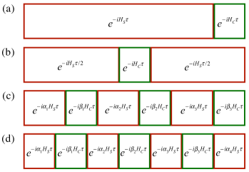
Figure 1: Illustration of the sliced time evolution operator using different orders of the Trotter decomposition. (a) First order. (b) Second order. (c) Third order. The parameters are $\alpha_{1}=1-\gamma,\beta_{1}={(4/3-\gamma\pm\Gamma)}/[{2\gamma}(\gamma\pm\Gamma)],\alpha_{2}=(\gamma\pm\Gamma)/2,\beta_{2}=(3-4\gamma)/[2(2-3\gamma)],\alpha_{3}=(\gamma\mp\Gamma)/2,\beta_{3}=1-(3\gamma-4/3\mp\Gamma)/[2\gamma(\gamma\mp\Gamma)]$, and $\Gamma=[\left(-12\gamma^{3}+45\gamma^{2}-48\gamma+16\right)/(-12\gamma+9)]^{1/2}$ with $\gamma$ being an arbitrary number. (d) Fourth order. The parameters are $\alpha_{1}=\alpha_{4}=\beta_{1}/2,\alpha_{2}=\alpha_{3}=(1-\beta_{1})/2$, and $\beta_{1}=\beta_{3}=1/(2-\sqrt[3]{2}),\beta_{2}=-\sqrt[3]{2}\beta_{1}$.

II Framework

We consider an $n$-qubit quantum system which is described by the system Hamiltonian $H_{S}$. In order to realize a desired quantum state or quantum operation, we apply the time-dependent controls along $x$ and $y$ directions, i.e., $u(t)=(u_{x}^{j}(t),u_{y}^{j}(t))$, where $j=1,2,...,n$ and $t\in[0,T]$ with $T$ being the total time length of the pulse. As such, the control Hamiltonian is written as

$$H_{C}(t)=\sum_{j=1}^{n}\left[u_{x}^{j}(t)\sigma_{x}^{j}+u_{y}^{j}(t)\sigma_{y}^{j}\right],$$ (1)

where $\sigma_{x}^{j}$ and $\sigma_{y}^{j}$ are the Pauli operators for the $j$th qubit. For a given time $T$, the time evolution operator of this coherently controlled quantum system is

$$U(T)=\mathcal{T}\exp\left\{-i\int_{0}^{T}\left[H_{S}+H_{C}(t)\right]dt\right\},$$ (2)

with $\mathcal{T}$ being the Dyson time-ordering operator. Generally, one is not able to directly evaluate this time-dependent exponential integral in an analytical way. The routine is to break down the continuously varying Hamiltonian into a discrete sequence. More precisely, the total evolution time $T$ is discretized into $M$ equal steps under the constraint that each duration $\tau=T/M$ is small enough, i.e., $\tau\ll\|H_{S}+H_{C}\|^{-1}$. As such, the control amplitude during each time duration $\tau$ can be regarded as constant, i.e., $u=(u_{x}^{j}[m],u_{y}^{j}[m])$, where $m$ runs from $1$ to $M$. After discretization, the control Hamiltonian at the $m$th step is $H_{C}[m]=\sum_{j=1}^{n}\left(u_{x}^{j}[m]\sigma_{x}^{j}+u_{y}^{j}[m]\sigma_{y}^{j}\right)$. Denoting the time evolution operator of the $m$th step as $U^{m}=e^{-i\tau\left(H_{S}+H_{C}[m]\right)}$, then the total evolution operator is $U_{0}(T)=U^{M}\cdots U^{1}$. According to the specific control target, one defines a suitable control performance function, such as state fidelity or gate fidelity, and then various optimization algorithms can be employed to search the optimal control pulse.

A critical difficulty that arises during the iterative optimization process is that evaluating the time evolution operators, which are matrix exponentials, may have exponential scaling of time and memory cost with respect to the number of qubits $n$. A similar difficulty that exists in quantum simulation is realizing the complex time evolution on real physical platforms, which can be greatly solved by the well-known Trotter decompositions [29, 30, 31]. It inspires us to use the Trotter decompositions to mitigate the issue of fully computing matrix exponentials in the iterative optimization process. Concretely, for small enough $\tau$, we can express the $m$th step evolution operator as follows:

$$e^{-i(H_{S}+H_{C}[m])\tau}=\prod_{k}e^{-i\alpha_{k}H_{S}\tau}e^{-i\beta_{k}H_{C}[m]\tau}+O(\tau^{l+1}),$$ (3)

where the parameters $\left\{\alpha_{k}\right\}$ and$\left\{\beta_{k}\right\}$ are suitably chosen such that the right-hand side of the equation, referred to as the $l$th-order approximant, yields an error term of order $O(\tau^{l+1})$. Rigorous error analysis of the Trotter decompositions should resort to the recent work Ref. [32]. Generally speaking, the parameters $\left\{\alpha_{k}\right\}$ and$\left\{\beta_{k}\right\}$ can be designed symmetrically [33, 25, 27] or asymmetrically [34, 35, 36]. The asymmetric scheme makes it easier to realize higher-order decompositions with rational parameters, yet requires more splitting terms compared with the symmetric scheme for the approximant of the same order [35]. From the perspective of practicality, we thus choose the symmetric Trotter decompositions to approximate the time evolution operators. Specifically, with the simplest first-order decomposition, the system evolution operator can be approximated by

$$U_{1}(T)\approx\prod_{m=1}^{M}e^{-iH_{S}\tau}e^{-iH_{C}[m]\tau}.$$ (4)

Despite its simplicity, the resultant error can become significant as the control parameters grow. To tackle this problem, we propose to use the higher-order Trotter decompositions. For the widely known second-order decomposition, the total system evolution can be approximately calculated by

$$U_{2}(T)\approx\prod_{m=1}^{M}e^{-iH_{S}\tau/2}e^{-iH_{C}[m]\tau}e^{-iH_{S}\tau/2}.$$ (5)

Similarly, the approximate system evolution operator for the third-order decomposition is

$$U_{3}(T)\approx{} \prod_{m=1}^{M}e^{-i\alpha_{1}H_{S}\tau}e^{-i\beta_{1}H_{C}[m]\tau}e^{-i\alpha_{2}H_{S}\tau}$$ (6)

$$e^{-i\beta_{2}H_{C}[m]\tau}e^{-i\alpha_{3}H_{S}\tau}e^{-i\beta_{3}H_{C}[m]\tau},$$

and for the fourth-order decomposition is

$$U_{4}(T)\approx{} \prod_{m=1}^{M}e^{-i\alpha_{1}H_{S}\tau}e^{-i\beta_{1}H_{C}[m]\tau}e^{-i\alpha_{2}H_{S}\tau}$$ (7)

$$e^{-i\beta_{2}H_{C}[m]\tau}e^{-i\alpha_{3}H_{S}\tau}e^{-i\beta_{3}H_{C}[m]\tau}e^{-i\alpha_{4}H_{S}\tau}.$$

See Fig. 1 for the illustration of the first-order to the fourth-order Trotter decompositions and the corresponding parameters $\left\{\alpha_{k}\right\}$ and$\left\{\beta_{k}\right\}$. In this way, we split the system Hamiltonian and the control Hamiltonian into separate evolution operators. As the system evolution segments remain unchanged during the optimization, they only need to be calculated once. Additionally, the control evolution segments are actually single-qubit operations; though renewed iteratively, they are easy to compute and store. We thus anticipate that this strategy can reduce the resources needed to compute the complex time evolution operator during the search of optimal control fields.

To figure out in which situations our strategy would likely be efficient, we provide rough analysis of the computational complexity. Generally, matrix exponential and matrix multiplication of full matrices both have the computational complexity of $O(N^{3})$ with $N=2^{n}$ [10, 37]. Our strategy breaks the full time evolution operator into several sparse matrix exponentials, thus the computational complexity of each matrix exponential may reduce to $O(N^{2})$ [10, 37]. However, the increased multiplication terms will certainly decrease the computing speed as the matrix multiplication is also resource consuming. Overall, our strategy can only get modest speed gains up to several times, and is mostly favorable for large quantum systems.

III Applications

As a demonstration, we first test the proposed strategy with the random Ising model [38] under transverse controls. The system Hamiltonian is set to be $H_{S}=\sum_{j=1}^{n-1}r_{1}^{j}\sigma_{z}^{j}\sigma_{z}^{j+1}$, where $r^{1}_{j}$ is the coefficient randomly chosen from the range $[0,1]$. The control Hamiltonian is expressed as $H_{C}[m]=\sum_{j=1}^{n}(r_{2}^{j}[m]\sigma_{x}^{j}+r_{3}^{j}[m]\sigma_{y}^{j})$ with $r_{2}^{j}[m]$ and $r_{3}^{j}[m]$ being random values in the range $[-1,1]$. We record the computer run time required to simulate the system evolution with and without using the Trotterization technique of different orders given by Eqs. (4)-(7). Meanwhile, we record the infidelity between the evolution operators simulated by the direct exponential operation ($U_{0}$) and the Trotter decompositions ($U_{l}$), i.e., $1-|\text{Tr}(U_{l}U_{0}^{\dagger})|^{2}/4^{n}$. The corresponding results are shown in Fig. 2.

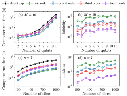
Figure 2: Computer run time and infidelity ($1-$fidelity) for simulating the system evolution of the controlled random Ising model. (a)-(b) For each qubit number $n$, the simulations are repeated ten times with different orders of the Trotterization to display the statistical errors, where $\tau=0.1,M=10$. (c)-(d) For the settled qubit number $n=7$ and $\tau=0.1$, the simulations for each sliced number $M$ are repeated ten times with different orders of the Trotterization to display the statistical errors.

For the case of varying the qubit number $n$ shown in Fig. 2(a), it is clear that using the first-order or the second-order Trotterization can greatly save the computing time, up to $50\%$ for $n=$ 2-4, and around $70$ to $90\%$ for $n=$ 5-11, while using the third-order or the fourth-order Trotterization only saves the computer run time significantly for the cases $n=$ 5-11, around $45$ to $65\%$. Nevertheless, as depicted in Fig. 2(b), the lower-order Trotterizations introduce more computational errors than the higher-order Trotterizations, thus the trade-off between accuracy and computing speed should be taken into consideration, which we will explore later. It is worth mentioning that, owing to the memory and speed limit of the personal computer, we only simulate up to $11$ qubits with $M=10$; further simulations towards larger systems with more sliced numbers should resort to powerful supercomputers. However, in many practical situations, reliable dynamical simulations often need to discretize the time evolution into hundreds of segments, thus it is necessary to investigate the behaviors of the proposed and the conventional strategy with varied number of slices. Here, we take $n=7$ as an example to show their behaviors in Figs. 2(c) and 2(d). One can find that as $M$ grows, the computing time of simulating the system evolution using the Trotterizations uniformly decreases, more than $80\%$ with the first-order or the second-order Trotterization, and more than $50\%$ with the third-order or the fourth-order Trotterization. Additionally, the computational errors gradually increase as $M$ grows, which should be carefully considered in specific situations.

The above demonstration, though simple and direct, clearly reveals the effectiveness of the Trotterization technique on reducing the computational resources. In the following, we consider two realistic applications of searching optimal control fields using the proposed strategy.

1 Improved GRAPE for pulse optimization

The GRAPE algorithm [6], which exploits the gradient information of an objective function to update the control fields iteratively, is a well-known optimization algorithm to tackle quantum state engineering and quantum gate preparation problems. First developed for designing nuclear magnetic resonance (NMR) pulses, it is also widely used in electron-spin resonance [39], nitrogen-vacancy centers in diamond [40, 41], superconducting circuits [42, 43], ion traps [44, 45], cold atoms [46], etc. Normally, we first formulate an objective function $f(u)$ to assess the candidate control fields. GRAPE then finds local extrema of control solutions by taking steps along the gradient direction, i.e., $u^{(p+1)}=u^{(p)}+\lambda^{(p)}g^{(p)}$, where $p$ represents the iteration number, $\lambda^{(p)}$ is an appropriate step length and the gradient $g^{(p)}=(g_{x}^{j}[m]^{(p)},g_{y}^{j}[m]^{(p)})$ with $g_{\gamma}^{j}[m]^{(p)}=\partial f^{(p)}/\partial u_{\gamma}^{j}[m]^{(p)}$ for $\gamma=x,y$. To accelerate the convergence speed, we apply the second-order quasi-Newton method, which approximates the actual Hessian with the gradient information computed from previous steps [47, 48]. More precisely, this is achieved by using the Limited-memory Broyden–Fletcher–Goldfarb–Shanno (LBFGS) method in Matlab, which further optimizes the optimization procedure with limited memory [49]. Clearly, in the process of calculating the objective function $f$ and its approximate Hessian, a considerable number of matrix exponentials of the time evolution segments need to be done, which would cost an exponential amount of computer run time. Furthermore, these time evolution segments must be re-evaluated in each iteration for the renewed control parameters, making the algorithm quickly intractable for even modest-sized quantum optimal control problems. Thus it is desirable to develop more efficient strategies to simulate the system evolution here. It is worth noting that Ref. [28] has concisely discussed how to use the first- and the second-order Trotterizations to improve the basic GRAPE algorithm. Our applications here explore in detail the performance of the high-order Trotterizations in pulse optimization with the second-order GRAPE algorithm.

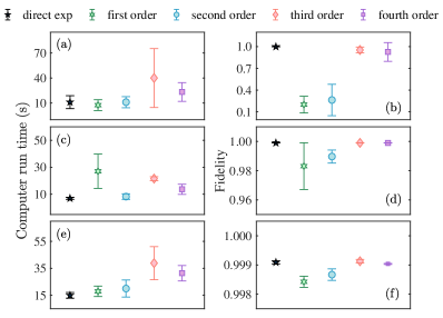
Figure 3: The GRAPE algorithm with the Trotterizations for searching optimal pulses to prepare the four-qubit GHZ state. The total evolution time $T=5~{}$ms, which is divided into different number of slices: (a)-(b) $M=200$; (c)-(d) $M=500$; (e)-(f) $M=1000$. The optimization is terminated when the estimated fidelity $f_{l}>0.999$ or the iteration number $p>1000$. The computer run time and the final true fidelity $f$ are recorded. The optimizations are all repeated five times to display the statistical errors.

To give a concrete example, consider the control optimization problem of preparing the known Greenberger-Horne-Zeilinger (GHZ) state [50] in a four-qubit NMR system. The natural Hamiltonian can be expressed as $H_{S}=-\sum_{i=1}^{4}{\omega_{i}}\sigma^{i}_{z}/2+\sum_{i<j,=1}^{4}{\pi J_{ij}}\sigma^{i}_{z}\sigma^{j}_{z}/2$, where $\omega_{i}$ represents the Larmor precession frequency for the $i$th spin and $J_{ij}$ is the $J$-coupling constant between the $i$th and the $j$th spin. The strengths of the Larmor frequencies and the $J$ couplings can be found in Ref. [51]. The four-qubit GHZ state takes the form $|\psi_{\text{GHZ}}\rangle=(|0\rangle^{\otimes 4}+|1\rangle^{\otimes 4})/\sqrt{2}$. The goal is to find an optimal control pulse $u_{\text{opt}}$ that can steer the system from $|\psi_{0}\rangle=|0\rangle^{\otimes 4}$ to $|\psi_{\text{GHZ}}\rangle$, with maximizing the state fidelity defined as $f_{l}=\left|\langle\psi_{\text{GHZ}}|U_{l}|\psi_{0}\rangle\right|^{2}$. Combining the Trotterization technique with GRAPE gives a way to find the optimal control fields; a similar work is found in Ref. [28]. However, the Trotterization technique may introduce significant errors in simulating the system evolution, thus we check the true fidelity of the discovered optimal controls by $f=\left|\langle\psi_{\text{GHZ}}|U_{0}(u_{\text{opt}})|\psi_{0}\rangle\right|^{2}$. The computer run time and the true fidelity using different orders of the Trotterization are shown in Fig. 3. We fix the total evolution time as $T=5~{}$ ms with different number of slices in the optimizations. For the first-order and the second-order Trotterization, if $M=200$, it can slightly save the computing time, yet introducing very large computational errors [see Figs. 3(a) and 3(b)]. Increasing the sliced number $M$ can improve the true fidelity [Figs. 3(d) and 3(f)], but cost around 18-286% more computing time [Figs. 3(c) and 3(e)]. For the third-order and the fourth-order Trotterization, though they always induce very high true fidelity beyond 0.99, and around 85-264% more computing time is needed. In total, the Trotterization technique does not provide speedup for the GRAPE algorithm in a small-scale system, which is consistent with the results shown in Fig. 2. The reason behind this is that matrix exponential and matrix multiplication both generally scale as $O(N^{3})$ with $N=2^{n}$. Though the splitting terms using the Trotterization may scale as $O(N^{2})$, the increased multiplications will reduce the computing speed. Thus for a small-scale system, the Trotterization based GRAPE algorithm may fail to achieve speed gains.

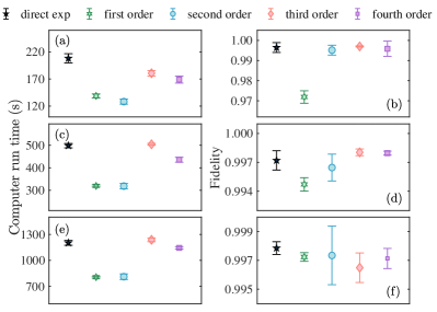
Figure 4: The GRAPE algorithm with the Trotterizations for searching optimal pulses to realize single-qubit rotation in a seven-qubit system. The total evolution time $T=1~{}$ms, which is divided into different number of slices: (a)-(b) $M=100$; (c)-(d) $M=250$; (e)-(f) $M=500$. We stop the optimization when the estimated fidelity $f_{l}>0.999$ or the iteration number $p$ exceeds $500$, and record the computer run time and the final true fidelity $f$ for each case. The optimizations are all repeated five times to display the statistical errors.

Now we turn to consider the problem of finding optimal pulses for achieving single-qubit rotation in a seven-qubit NMR system. The natural Hamiltonian is $H_{S}=-\sum_{i=1}^{7}{\omega_{i}}\sigma^{i}_{z}/2+\sum_{i<j,=1}^{7}{\pi J_{ij}}\sigma^{i}_{z}\sigma^{j}_{z}/2$, and the strengths of the Larmor frequencies and the $J$ couplings can be found in Ref. [23]. Our goal is to search out an optimal control pulse $u_{\text{opt}}$ that can steer the system to achieve the target single-qubit operation $U_{t}=\exp(-i\pi\sigma^{2}_{x}/4)$, with maximizing the gate fidelity $f_{l}=|\text{Tr}(U_{l}U_{t}^{\dagger})|^{2}/4^{7}$. Similarly, we combine the Trotterization technique with the GRAPE algorithm to accomplish this optimization task, and we check the final true fidelity of the searched optimal controls with $f=|\text{Tr}(U_{0}(u_{\text{opt}})U_{t}^{\dagger})|^{2}/4^{7}$. We fix the total evolution time as $T=1~{}$ ms with different number of slices in the optimizations. For the case of $M=100$ shown in Figs. 4(a) and 4(b), using the first-order to the fourth-order Trotterization can save the computing time about 33, 38, 13, and 19%, respectively. However, the final true gate fidelities using the first-order and the second-order Trotterization are roughly smaller than 0.99, which is often below the fault-tolerant threshold [52]. Increasing $M$ to 250, as shown in Figs. 4(c) and 4(d), the final gate fidelities are all beyond 0.994, and the first-order to the fourth-order Trotterization can save the computing time about 36, 36, -1, and 12%, respectively. For much larger sliced number $M=500$ shown in Figs. 4(e) and 4(f), their true fidelities are all beyond 0.995 and the corresponding reduced computing time is about 33, 32, -3, and 5%, respectively. These results indicate that using the first-order and the second-order Trotterization can always significantly save the computing time, but only achieve sufficient high fidelity when the duration time $\tau=T/M$ is small enough. Meanwhile, using the third-order and the fourth-order Trotterization can achieve very high fidelity even when $\tau$ is relatively large, but may not save that much computing time. In total, these results indicate that our proposed strategy is mostly favorable for a relatively large system, and it can possibly save much more computer run time when searching optimal pulses for intermediate-scale optimization tasks.

To further exploit the potential of the proposed strategy, we attempt to use hybrid Trotterizations to improve the performance of the GRAPE. Precisely, we apply the low-order Trotterization in the early stages of GRAPE and the switch to the high-order Trotterization in the final stages. To test this hybrid strategy, the specific problem we choose is the same as above, namely, finding optimal pulses for realizing single-qubit rotation in a seven-qubit NMR system. In the simulations, we use the first-order or the second-order Trotterization during the former 400 iterations and then switch to the third-order or the fourth-order Trotterization during the latter 100 iterations. The simulation results are shown in Fig. 5. Compared with the first-order Trotterization, it is clear that the hybrid first- to third-order and first- to fourth-order Trotterization significantly increase the fidelity from 0.972 to 0.993, nearly without costing more computer run time, while, compared with second-order Trotterization, the hybrid second- to third-order and second- to fourth-order Trotterization can slightly increase the fidelity from 0.995 to 0.997, but cost 30-40% more computer run time. These results reveal that with proper hybrid Trotterizations, the performance of the GRAPE algorithm can be further improved.

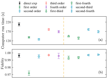
Figure 5: The GRAPE algorithm with different Trotterization strategies for searching optimal pulses to realize single-qubit rotation in a seven-qubit system, where $T=1$ and $M=100$. (a) and (b) display the computer run time and the fidelity for different Trotterization strategies, respectively. The panels on the right of the yellow dashed lines represent the results using the hybrid Trotterization strategies. The stopping condition is that the estimated fidelity $f_{l}>0.999$ or the iteration number $p>500$.

2 Improved VQA for ground-state energy solving

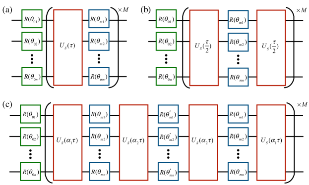
Figure 6: Efficient Ansätze inspired by the symmetric Trotterization for VQA. (a) Illustration of VQA based on the first-order Trotterization. This structure is also refereed to as a hardware-efficient Ansatz in Ref. [53]. (b) and (c) VQA based on the second-order and the symmetric fourth-order Trotterization, respectively, where $\alpha_{1}=s/2,\alpha_{2}=(1-s)/2,\theta_{jm}^{\prime}=-\sqrt[3]{2}\theta_{jm}$ with $s=1/(2-\sqrt[3]{2}),j=1,2,...,n$. In all the figures, $U_{S}(\tau)$ is the free evolution operator during the period $\tau$, which is governed by the available system Hamiltonian $H_{S}$, i.e., $U_{S}(\tau)=\exp(-iH_{S}\tau)$. Each single-qubit rotation is represented by $R(\theta_{mj})$ with the angle $\theta_{mj}$, and the rotation axis is typically chosen as $x$ axis and $y$ axis.

The VQA [54, 55], which functions by minimizing certain cost functions via the variation of limited gate parameters with low-depth circuits, has found tremendous applications in quantum chemistry, quantum simulation and machine learning [55]. Usually, the VQA first parametrizes a quantum circuit $U(\bm{\theta})$ with multiple layers of building blocks (called Ansatz), with each block involving single-qubit rotations and available non-local gates. Suitable optimization algorithms are then applied to tune the parameters $\bm{\theta}$ for minimizing the target cost function. The structure of an Ansatz is generally designed according to the optimization task at hand, but it can also be formalized when no relevant information is readily known. A notable example hardware-efficient Ansatz [53] (see Fig. 6(a)), which utilizes available entangling resources in a given physical device, is prominent for problem-agnostic situations.

Here, we find that the hardware-efficient Ansatz actually has a strong relationship with the sliced time evolution simulated by the first-order Trotterization. To be specific, the $m$th sliced evolution can be equivalently expressed as

$$U_{m}\approx e^{-iH_{S}\tau}e^{-iH_{C}[m]\tau}\equiv e^{-iH_{S}\tau}\cdot\bigotimes_{j=1}^{n}R({\theta}_{mj}),$$ (8)

where the control Hamiltonian part is the product of generic single-qubit rotations represented by

$$R(\theta_{mj})=R_{x}(\theta_{mj}^{1})R_{y}(\theta_{mj}^{2})R_{x}(\theta_{mj}^{3}),$$ (9)

and $R_{\gamma}(\theta_{mj}^{w})=\exp(-i\theta_{mj}^{w}\sigma_{\gamma}^{j}/2),\gamma=x,y;w=1,2,3$. Following similar mapping rules, we propose Ansätze based on the second-order and the fourth-order symmetric Trotterization [25, 26, 27], as shown in Figs. 6(b) and 6(c). For example, for the second-order Trotterization, the $m$th sliced evolution operator can be written as

$$U_{m} \approx e^{-iH_{S}\tau/2}e^{-iH_{C}[m]\tau}e^{-iH_{S}\tau/2}$$

$$=e^{-iH_{S}\tau/2}\cdot\bigotimes_{j=1}^{n}R({\theta}_{mj})\cdot e^{-iH_{S}\tau/2}.$$ (10)

As such, the whole evolution becomes a parametrized quantum circuit as shown in Fig. 6(b). A similar second-order Trotterization based Ansatz has been used in Ref. [56], and recent works [57, 58] also provide insights into informing the VQA with the quantum optimal control perspective. As we have analyzed that the higher-order Trotterizations can help improve the efficiency of simulating system evolution, we thus expect that the proposed new Ansätze function in improving the VQA. Additionally, it should be noted that for all the proposed Ansätze, the overall free evolution time in each block is $\tau$ , and the total number of parameters is $3(M+1)n$. This indicates that the higher-order Trotterization inspired Ansätze will not introduce extra computational and operational burdens.

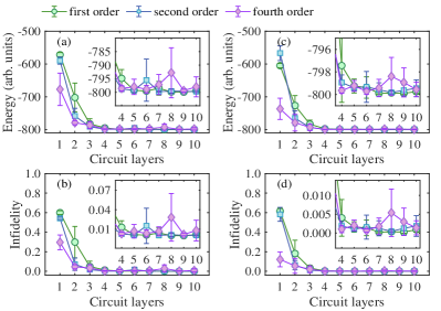
Figure 7: The Trotterization inspired VQA for solving the ground-state energy in the four-qubit Heisenberg model on a square lattice. Minimal energy found using VQA of different circuit layers when (a) $\tau=0.005~{}$s; (c) $\tau=0.01~{}$s. Corresponding state infidelity between the searched optimal ground state and the theoretical ground state when (b) $\tau=0.005~{}$s; (d) $\tau=0.01~{}$s. The optimization stops when the maximal iteration number exceeds 1000, and for each circuit layer the optimizations are repeated five times to display the statistical errors.

As a demonstration, we consider the problem of solving the ground-state energy in a four-qubit Heisenberg spin model on a square lattice [53]. This typical model has been widely explored in quantum areas, from thermodynamics and statistics to communication and computation [59, 60, 61], which can be realized by various physical systems [62, 63], such as ultracold atoms, trapped ions, and nuclear magnetic resonance. This model can be described by

$$H_{P}=J\sum_{\langle ij\rangle}\left(\sigma_{x}^{i}\sigma_{x}^{j}+\sigma_{y}^{i}\sigma_{y}^{j}+\sigma_{z}^{i}\sigma_{z}^{j}\right)+B_{z}\sum_{i}\sigma_{z}^{i},$$ (11)

where $J$ is the nearest-neighbor interaction strength, and $B_{z}$ is the longitudinal static field. With loss of generality, we set $J=100,B_{z}=100$.

To tackle this eigensolver problem, we use a four-spin NMR processor to generate candidate states from $\rho_{0}=|0\rangle^{\otimes 4}$ with the Trotterization inspired VQA. We then iteratively update the parameters to minimize the energy $f=\text{Tr}(H_{P}U(\bm{\theta})\rho_{0}U(\bm{\theta})^{\dagger})$ using the improved Nelder-Mead algorithm [64]. The natural Hamiltonian of this NMR processor is $H_{S}=-\sum_{i=1}^{4}{\omega_{i}}\sigma^{i}_{z}/2+\sum_{i<j,=1}^{4}{\pi J_{ij}}\sigma^{i}_{z}\sigma^{j}_{z}/2$, where $\omega_{i}$ represents the Larmor precession frequency for the $i$th spin and $J_{ij}$ is the $J$-coupling constant between the $i$th and the $j$th spin. The strengths of the Larmor frequencies and the $J$ couplings can be found in Ref. [51]. With different circuit layers, we show the numerical energy optimization results in Figs. 7(a) and 7(c). By defining the state fidelity between the searched ground state and the theoretical ground state $F=\text{Tr}(\rho_{th}U(\bm{\theta})\rho_{0}U(\bm{\theta})^{\dagger})$, we also display the corresponding state infidelity ($1-F$) in Figs. 7(b) and 7(d). These numerical results indicate that for small number of circuit layers $M=$ 1-3, the second-order and the fourth-order Trotterization inspired Ansätze perform much better than the hardware-efficient Ansatz. When increasing the circuit layers ($M>3$), the second-order Trotterization and the fourth-order Trotterization inspired Ansätze will have comparable performance with the hardware-efficient Ansatz. This is reasonable because for a limited number of circuit layers $M$, the higher-order Trotter decompositions possess higher precision to simulate the system evolution than the conventional hardware-efficient Ansatz. However, when $M$ is sufficiently large, the computational resources will be enough for all orders of the Trotter decompositions to achieve accurate results. This indicates that the proposed Ansätze are favorable for the highly short-depth VQA to find approximate solutions.

IV Conclusion and discussion

In the design of precise quantum control, simulating the system time evolution is the most resource-consuming part. To mitigate this issue, we combine the Trotter decompositions to propose a practical strategy suitable for various control optimization problems. The demonstrations with the GRAPE algorithm up to seven qubits show the effectiveness of our strategy in reducing the computing time. We expect that this strategy can be explored in an intermediate-scale system in the future, probably combining parallelization technique [20] or special matrix representation method [65]. Several new Ansätze inspired by the Trotter decompositions are also presented for improving the performance of the VQA, showing the advantages of finding approximate solutions with highly low-depth circuits. Actually, this is favorable for realistic applications, as current quantum devices often process many noisy qubits with a limited coherence time [66]. Furthermore, future investigations can explore the possibility of implementing the proposed strategy in more complex optimization and simulation tasks.

References

- Warren et al. [1993] W. S. Warren, H. Rabitz, and M. Dahleh, Coherent Control of Quantum Dynamics: The Dream Is Alive, Science 259, 1581 (1993).
- Brif et al. [2010] C. Brif, R. Chakrabarti, and H. Rabitz, Control of quantum phenomena: past, present and future, New J. Phys. 12, 075008 (2010).
- Koch et al. [2022] C. P. Koch, U. Boscain, T. Calarco, G. Dirr, S. Filipp, S. J. Glaser, R. Kosloff, S. Montangero, T. Schulte-Herbrüggen, D. Sugny, et al., Quantum optimal control in quantum technologies. Strategic report on current status, visions and goals for research in europe, EPJ Quantum Technol. 9, 19 (2022).
- Boscain et al. [2021] U. Boscain, M. Sigalotti, and D. Sugny, Introduction to the Pontryagin Maximum Principle for Quantum Optimal Control, PRX Quantum 2, 030203 (2021).
- d’Alessandro [2007] D. d’Alessandro, Introduction to Quantum Control and Dynamics (CRC Press, New York, 2007).
- Khaneja et al. [2005] N. Khaneja, T. Reiss, C. Kehlet, T. Schulte-Herbrüggen, and S. J. Glaser, Optimal control of coupled spin dynamics: design of nmr pulse sequences by gradient ascent algorithms, J. Magn. Reson. 172, 296 (2005).
- Zahedinejad et al. [2016] E. Zahedinejad, J. Ghosh, and B. C. Sanders, Designing High-Fidelity Single-Shot Three-Qubit Gates: A Machine-Learning Approach, Phys. Rev. Applied 6, 054005 (2016).
- Yang et al. [2019] X. Yang, J. Li, and X. Peng, An improved differential evolution algorithm for learning high-fidelity quantum controls, Sci. Bull. 64, 1402 (2019).
- Riaz et al. [2019] B. Riaz, C. Shuang, and S. Qamar, Optimal control methods for quantum gate preparation: a comparative study, Quantum Inf. Proc. 18, 100 (2019).
- Moler and Van Loan [2003] C. Moler and C. Van Loan, Nineteen Dubious Ways to Compute the Exponential of a Matrix, Twenty-Five Years Later, SIAM review 45, 3 (2003).
- Preskill [2018] J. Preskill, Quantum Computing in the NISQ era and beyond, Quantum 2, 79 (2018).
- White [1992] S. R. White, Density matrix formulation for quantum renormalization groups, Phys. Rev. Lett. 69, 2863 (1992).
- Vidal [2003] G. Vidal, Efficient Classical Simulation of Slightly Entangled Quantum Computations, Phys. Rev. Lett. 91, 147902 (2003).
- Evenbly and Vidal [2015] G. Evenbly and G. Vidal, Tensor Network Renormalization, Phys. Rev. Lett. 115, 180405 (2015).
- Doria et al. [2011] P. Doria, T. Calarco, and S. Montangero, Optimal Control Technique for Many-Body Quantum Dynamics, Phys. Rev. Lett. 106, 190501 (2011).
- Ryan et al. [2008] C. A. Ryan, C. Negrevergne, M. Laforest, E. Knill, and R. Laflamme, Liquid-state nuclear magnetic resonance as a testbed for developing quantum control methods, Phys. Rev. A 78, 012328 (2008).
- [17] J. Li, Subsystem-based approach to scalable quantum optimal control, arXiv:1910.02061 .
- Berry et al. [2015] D. W. Berry, A. M. Childs, R. Cleve, R. Kothari, and R. D. Somma, Simulating Hamiltonian Dynamics with a Truncated Taylor Series, Phys. Rev. Lett. 114, 090502 (2015).
- Kieferová et al. [2019] M. Kieferová, A. Scherer, and D. W. Berry, Simulating the dynamics of time-dependent hamiltonians with a truncated dyson series, Phys. Rev. A 99, 042314 (2019).
- Gradl et al. [2006] T. Gradl, A. Spörl, T. Huckle, S. J. Glaser, and T. Schulte-Herbrüggen, Parallelising matrix operations on clusters for an optimal control-based quantum compiler, in European Conference on Parallel Processing (Springer, 2006) pp. 751–762.
- Edwards and Kuprov [2012] L. J. Edwards and I. Kuprov, Parallel density matrix propagation in spin dynamics simulations, J. Chem. Phys. 136, 044108 (2012).
- Riahi et al. [2016] M. K. Riahi, J. Salomon, S. J. Glaser, and D. Sugny, Fully efficient time-parallelized quantum optimal control algorithm, Phys. Rev. A 93, 043410 (2016).
- Li et al. [2017] J. Li, X. Yang, X. Peng, and C.-P. Sun, Hybrid Quantum-Classical Approach to Quantum Optimal Control, Phys. Rev. Lett. 118, 150503 (2017).
- Lu et al. [2017] D. Lu, K. Li, J. Li, H. Katiyar, A. J. Park, G. Feng, T. Xin, H. Li, G. Long, A. Brodutch, B. Zeng, and R. Laflamme, Enhancing quantum control by bootstrapping a quantum processor of 12 qubits, npj Quantum Inf. 3, 45 (2017).
- Janke and Sauer [1992] W. Janke and T. Sauer, Properties of higher-order trotter formulas, Phys. Lett. A 165, 199 (1992).
- Kobayashi et al. [1994] H. Kobayashi, N. Hatano, and M. Suzuki, Study of correction terms for higher-order decompositions of exponential operators, Physica A 211, 234 (1994).
- Hatano and Suzuki [2005] N. Hatano and M. Suzuki, Finding exponential product formulas of higher orders, in Quantum annealing and other optimization methods (Springer, 2005) pp. 37–68.
- Bhole and Jones [2018] G. Bhole and J. A. Jones, Practical pulse engineering: Gradient ascent without matrix exponentiation, Front. Phys. 13, 130312 (2018).
- Suzuki [1976] M. Suzuki, Generalized trotter’s formula and systematic approximants of exponential operators and inner derivations with applications to many-body problems, Commun.Math. Phys. 51, 183 (1976).
- Suzuki [1985] M. Suzuki, Decomposition formulas of exponential operators and lie exponentials with some applications to quantum mechanics and statistical physics, J. Math. Phys. 26, 601 (1985).
- Georgescu et al. [2014] I. M. Georgescu, S. Ashhab, and F. Nori, Quantum simulation, Rev. Mod. Phys. 86, 153 (2014).
- Childs et al. [2021] A. M. Childs, Y. Su, M. C. Tran, N. Wiebe, and S. Zhu, Theory of Trotter Error with Commutator Scaling, Phys. Rev. X 11, 011020 (2021).
- Suzuki [1992a] M. Suzuki, General theory of higher-order decomposition of exponential operators and symplectic integrators, Phys. Lett. A 165, 387 (1992a).
- Ruth [1983] R. D. Ruth, A canonical integration technique, IEEE Trans. Nucl. Sci. 30, 2669 (1983).
- Suzuki [1992b] M. Suzuki, General nonsymmetric higher-order decomposition of exponential operators and symplectic integrators, J. Phys. Soc. Japan 61, 3015 (1992b).
- Liu et al. [2020] Y.-X. Liu, J. Hines, Z. Li, A. Ajoy, and P. Cappellaro, High-fidelity trotter formulas for digital quantum simulation, Phys. Rev. A 102, 010601 (2020).
- Stothers [2010] A. J. Stothers, On the complexity of matrix multiplication (Ph.D. Thesis, the university of Edinburgh, 2010) .
- Friedenauer et al. [2008] A. Friedenauer, H. Schmitz, J. T. Glueckert, D. Porras, and T. Schätz, Simulating a quantum magnet with trapped ions, Nat. Phys. 4, 757 (2008).
- Zhang et al. [2011] Y. Zhang, C. A. Ryan, R. Laflamme, and J. Baugh, Coherent Control of Two Nuclear Spins Using the Anisotropic Hyperfine Interaction, Phys. Rev. Lett. 107, 170503 (2011).
- Waldherr et al. [2014] G. Waldherr, Y. Wang, S. Zaiser, M. Jamali, T. Schulte-Herbrüggen, H. Abe, T. Ohshima, J. Isoya, J. Du, P. Neumann, and J. Wrachtrup, Quantum error correction in a solid-state hybrid spin register, Nature 506, 204 (2014).
- Dolde et al. [2014] F. Dolde, V. Bergholm, Y. Wang, I. Jakobi, B. Naydenov, S. Pezzagna, J. Meijer, F. Jelezko, P. Neumann, T. Schulte-Herbrüggen, J. Biamonte, and J. Wrachtrup, High-fidelity spin entanglement using optimal control, Nat. Commun. 5, 3371 (2014).
- Motzoi et al. [2009] F. Motzoi, J. M. Gambetta, P. Rebentrost, and F. K. Wilhelm, Simple Pulses for Elimination of Leakage in Weakly Nonlinear Qubits, Phys. Rev. Lett. 103, 110501 (2009).
- Egger and Wilhelm [2014] D. J. Egger and F. K. Wilhelm, Optimized controlled-z gates for two superconducting qubits coupled through a resonator, Supercond. Sci. Technol. 27, 014001 (2014).
- Nebendahl et al. [2009] V. Nebendahl, H. Häffner, and C. F. Roos, Optimal control of entangling operations for trapped-ion quantum computing, Phys. Rev. A 79, 012312 (2009).
- Schindler et al. [2011] P. Schindler, J. T. Barreiro, T. Monz, V. Nebendahl, D. Nigg, M. Chwalla, M. Hennrich, and R. Blatt, Experimental repetitive quantum error correction, Science 332, 1059 (2011).
- Saywell et al. [2018] J. C. Saywell, I. Kuprov, D. Goodwin, M. Carey, and T. Freegarde, Optimal control of mirror pulses for cold-atom interferometry, Phys. Rev. A 98, 023625 (2018).
- Machnes et al. [2011] S. Machnes, U. Sander, S. J. Glaser, P. de Fouquières, A. Gruslys, S. Schirmer, and T. Schulte-Herbrüggen, Comparing, optimizing, and benchmarking quantum-control algorithms in a unifying programming framework, Phys. Rev. A 84, 022305 (2011).
- de Fouquieres et al. [2011] P. de Fouquieres, S. G. Schirmer, S. J. Glaser, and I. Kuprov, Second order gradient ascent pulse engineering, J. Magn. Reson. 212, 412 (2011).
- Liu and Nocedal [1989] D. C. Liu and J. Nocedal, On the limited memory bfgs method for large scale optimization, Math. Program. 45, 503 (1989).
- Pezzè et al. [2018] L. Pezzè, A. Smerzi, M. K. Oberthaler, R. Schmied, and P. Treutlein, Quantum metrology with nonclassical states of atomic ensembles, Rev. Mod. Phys. 90, 035005 (2018).
- Zhou et al. [2020] H. Zhou, Y. Ji, X. Nie, X. Yang, X. Chen, J. Bian, and X. Peng, Experimental Realization of Shortcuts to Adiabaticity in a Nonintegrable Spin Chain by Local Counterdiabatic Driving, Phys. Rev. Applied 13, 044059 (2020).
- Campbell et al. [2017] E. T. Campbell, B. M. Terhal, and C. Vuillot, Roads towards fault-tolerant universal quantum computation, Nature 549, 172 (2017).
- Kandala et al. [2017] A. Kandala, A. Mezzacapo, K. Temme, M. Takita, M. Brink, J. M. Chow, and J. M. Gambetta, Hardware-efficient variational quantum eigensolver for small molecules and quantum magnets, Nature 549, 242 (2017).
- Moll et al. [2018] N. Moll, P. Barkoutsos, L. S. Bishop, J. M. Chow, A. Cross, D. J. Egger, S. Filipp, A. Fuhrer, J. M. Gambetta, M. Ganzhorn, A. Kandala, A. Mezzacapo, P. Müller, W. Riess, G. Salis, J. Smolin, I. Tavernelli, and K. Temme, Quantum optimization using variational algorithms on near-term quantum devices, Quantum Sci. Technol. 3, 030503 (2018).
- Cerezo et al. [2021] M. Cerezo, A. Arrasmith, R. Babbush, S. C. Benjamin, S. Endo, K. Fujii, J. R. McClean, K. Mitarai, X. Yuan, L. Cincio, et al., Variational quantum algorithms, Nat. Rev. Phys. 3, 625 (2021).
- Wecker et al. [2015] D. Wecker, M. B. Hastings, and M. Troyer, Progress towards practical quantum variational algorithms, Phys. Rev. A 92, 042303 (2015).
- Choquette et al. [2021] A. Choquette, A. Di Paolo, P. K. Barkoutsos, D. Sénéchal, I. Tavernelli, and A. Blais, Quantum-optimal-control-inspired ansatz for variational quantum algorithms, Phys. Rev. Research 3, 023092 (2021).
- Magann et al. [2021] A. B. Magann, C. Arenz, M. D. Grace, T.-S. Ho, R. L. Kosut, J. R. McClean, H. A. Rabitz, and M. Sarovar, From pulses to circuits and back again: A quantum optimal control perspective on variational quantum algorithms, PRX Quantum 2, 010101 (2021).
- Bañuls et al. [2011] M. C. Bañuls, J. I. Cirac, and M. B. Hastings, Strong and Weak Thermalization of Infinite Nonintegrable Quantum Systems, Phys. Rev. Lett. 106, 050405 (2011).
- Zueco et al. [2009] D. Zueco, F. Galve, S. Kohler, and P. Hänggi, Quantum router based on ac control of qubit chains, Phys. Rev. A 80, 042303 (2009).
- De Chiara et al. [2012] G. De Chiara, L. Lepori, M. Lewenstein, and A. Sanpera, Entanglement Spectrum, Critical Exponents, and Order Parameters in Quantum Spin Chains, Phys. Rev. Lett. 109, 237208 (2012).
- Simon et al. [2011] J. Simon, W. S. Bakr, M. E. T. R. Ma, P. M. Preiss, and M. Greiner, Quantum simulation of antiferromagnetic spin chains in an optical lattice, Nature 472, 307 (2011).
- Greif et al. [2013] D. Greif, T. Uehlinger, G. Jotzu, L. Tarruell, and T. Esslinger, Short-range quantum magnetism of ultracold fermions in an optical lattice, Science 340, 1307 (2013).
- Pham et al. [2011] N. Pham, A. Malinowski, and T. Bartczak, Comparative study of derivative free optimization algorithms, IEEE Trans. Industr. Inform. 7, 592 (2011).
- Hogben et al. [2010] H. Hogben, P. Hore, and I. Kuprov, Strategies for state space restriction in densely coupled spin systems with applications to spin chemistry, J. Chem. Phys. 132, 174101 (2010).
- Ladd et al. [2010] T. D. Ladd, F. Jelezko, R. Laflamme, Y. Nakamura, C. Monroe, and J. L. O’Brien, Quantum computers, Nature 464, 45 (2010).