Non-Stationary Bandit Learning via Predictive Sampling

Abstract

Thompson sampling has proven effective across a wide range of stationary bandit environments. However, as we demonstrate in this paper, it can perform poorly when applied to non-stationary environments. We attribute such failures to the fact that, when exploring, the algorithm does not differentiate actions based on how quickly the information acquired loses its usefulness due to non-stationarity. Building upon this insight, we propose predictive sampling, an algorithm that deprioritizes acquiring information that quickly loses usefulness. A theoretical guarantee on the performance of predictive sampling is established through a Bayesian regret bound. We provide versions of predictive sampling for which computations tractably scale to complex bandit environments of practical interest. Through numerical simulations, we demonstrate that predictive sampling outperforms Thompson sampling in all non-stationary environments examined.

1 Introduction

Thompson sampling (TS) (Thompson,, 1933) is a bandit learning algorithm that operates by sampling at each timestep statistically plausible mean rewards and selecting the action associated with the largest sample. For a range of stationary bandit environments, or stationary bandits, for short, the efficacy of TS has been established through theoretical and empirical analyses (Agrawal and Goyal,, 2012; Chapelle and Li,, 2011; Russo and Van Roy,, 2014). The algorithm has enjoyed a wide range of applications, including revenue management (Ferreira et al.,, 2018), website optimization (Hill et al.,, 2017), Monte Carlo tree search (Bai et al.,, 2013), A/B testing (Graepel et al.,, 2010), advertising (Agarwal et al.,, 2014; Graepel et al.,, 2010; Agarwal,, 2013; Schwartz et al.,, 2017), and recommender systems (Kawale et al.,, 2015).

Many of these applications, however, exhibit non-stationarity. For example, recommender systems often serve user populations where trends and preferences fluctuate over time. Similarly, learning algorithms designed for dynamic pricing can be impacted by seasonal changes in supply and demand patterns. Unfortunately, as we demonstrate in this paper, TS is not suited for these non-stationary environments. We show that applying TS can lead to near worst-case performance in some examples of non-stationary bandits; this is further corroborated by the sub-optimal performance of TS in our numerical experiments.

What causes TS to perform poorly in the face of non-stationarity? We believe that a main driver is its failure to account for information durability. In a stationary environment, because the reward distributions do not change over time, any information the agent gathers about the reward distribution of an action, say, its mean, remains useful till the end of the time horizon. In contrast, reward distributions change over time in a non-stationary environment, and information obtained in the past will gradually lose usefulness for predicting future rewards. To add to the complexity, reward distributions associated with different actions may evolve at different speeds, and consequently, so will the value of information acquired about these actions. To summarize, the presence of non-stationarity not only endows information with a finite durability, but such information durability may vary across actions.

The presence of information durability ought to change how an agent balances between maximizing current performance (exploitation) and obtaining new information about the quality of an action (exploitation). For one, we would probably expect a good agent to explore less those actions with poor information durability, because such investments, at best, could only help inform the agent’s decisions for a relative short period of time. Notably, the original TS algorithm differentiates actions only via their respective posterior reward distribution, and not by their information durability: two actions could have distinct levels of information durability, but identical or similar posterior reward distributions, and consequently TS would explore both actions with equal intensity. Our subsequent analyses and numerical experiments would further support the assessment that the inability to adjust exploration according to information durability lies at the heart of TS’s failure in non-stationary environments.

Motivated by the above observations, we propose in this paper predictive sampling (PS) as an effective algorithm for non-stationary bandit learning. At a high-level, PS inherits the same conceptual elegance of the original TS algorithm, but is redesigned in such way that naturally shapes exploration using information durability. Concretely, PS operates by sampling at each timestep a statistically plausible sequence of future rewards, before selecting the action that maximizes the expected reward conditioned on the sequence being the true future rewards. When the environment is stationary, we demonstrate that a PS agent and a TS agent execute the same policy. When the environment is non-stationary, however, we illustrate how PS, unlike TS, intelligently adjusts its intensity of exploration based the durability of information, giving it a clear advantage. We show that, in some extreme cases, PS can attain near optimal performance while TS suffers near worst-case performance.

A second major contribution of the present paper lies in establishing a general information-theoretic framework that is capable of analyzing the performance of any agent in a non-stationary bandit. The environment’s being non-stationary introduces significant challenges to applying existing information-theoretic analyses due to changes in both the quantity and the quality of information. For example, while the total amount of information in the environment is typically bounded in a stationary bandit, in a non-stationary one, additional randomness can be injected to the environment in each time step, and thus the information can grow unbounded as the horizon $T$ increases. Furthermore, as discussed earlier, not all of such information is relevant when it comes to predicting future rewards, so the analysis needs to tease out durable information and quantify its performance impact. To overcome these difficulties, we introduce a novel concept of predictive information, which captures the type of information that is useful in predicting future rewards. Using it, along with a new notion of information ratio, we are able to extend the information-theoretic regret analysis originally developed for stationary bandits (Russo and Van Roy,, 2014) to non-stationary bandit learning and obtain non-trivial regret upper bounds.

Using this framework, we establish a general regret bound for any agent that is expressed in terms of the cumulative predictive information $\Delta$. The bound grows linearly in $\sqrt{\Gamma\Delta}$, where $\Gamma$ denotes the sum of the information ratios. Applying this analysis to PS, we establish a regret bound that grows linearly in $\sqrt{T\Delta}$. In particular, when applied to a stationary environment, this bound reproduces some of the best known bounds for the regret of TS (c.f., (Neu et al.,, 2022)), suggesting that this new analysis is likely competitive against its stationary counterparts in terms of tightness.

We further leverage these general regret bounds to derive easy-to-interpret guarantees for specific classes of non-stationary bandit problems. We do so by developing new techniques that allow us to upper-bound the cumulative predictive information $\Delta$. For instance, we analyze a class of modulated Bernoulli bandits that generalizes the constant rate per-arm abrupt switching model in (Mellor and Shapiro,, 2013), where the reward distributions evolve according to a Markov chain. In this case, we are able to derive explicit bounds on $\Delta$ and further bounds on the regret that exhibits a graceful dependence on the transition kernel of the modulating Markov chain. We also establish a lower bound on the regret incurred by any agent in these bandits. These regret bounds demonstrate the effectiveness of predictive sampling across a range of such non-stationary Bernoulli bandits.

Finally, we develop computationally tractable implementations of PS. For a class of non-stationary Gaussian bandits, we demonstrate how to implement PS exactly in a computationally efficient manner. For a more complex class of non-stationary logistic bandits, where PS is too computationally expensive to be performed exactly, we develop an efficient procedure to approximate PS using Laplace approximation. Using these implementations, we conduct extensive numerical experiments across a range of such bandits with varying information durability. Our computational results suggest that PS, as well as its approximation, consistently outperform not only TS, but also other algorithms proposed for non-stationary bandit learning.

In summary, the main contributions of this paper include:

1. We elucidate how and why TS and variants of TS proposed in previous literature do not account for information durability when selecting actions.

2. We propose PS for non-stationary bandit learning, and layout qualitative insights on how and why PS can significantly outperform TS in non-stationary environments. We further support the claim with theoretical results and numerical evidence.

3. We develop computationally tractable implementations of PS for a class of Gaussian bandits which we refer to as AR(1) bandits and an approximation of PS for a class of logistic bandits.

Structure of the paper  The paper is organized as follows. Section 3 presents an example illustrating the limitations of TS in certain non-stationary bandits. Section 4 introduces a general formulation of bandits. Sections 5 and 6 formally introduce PS and discuss its qualitative properties. Section 7 provides the regret analyses. Section 8 presents tractable examples and approximations of PS, along with numerical experiments. Section 9 summarizes the paper. The appendix provides the probabilistic framework, information-theoretic notations and concepts, and technical proofs.

2 Related Work

Non-Stationary Bandit Learning

A number of interesting algorithms for non-stationary bandit learning have been proposed based on modifying TS (Ghatak,, 2021; Gupta et al.,, 2011; Mellor and Shapiro,, 2013; Raj and Kalyani,, 2017; Trovo et al.,, 2020; Viappiani,, 2013) or other stationary bandit algorithms (Besbes et al.,, 2019; Besson and Kaufmann,, 2019; Cheung et al.,, 2019; Garivier and Moulines,, 2008; Hartland et al.,, 2006; Kocsis and Szepesvári,, 2006; Mellor and Shapiro,, 2013). However, the majority of these algorithms focus on using structural knowledge of the non-stationarity to refine estimates of the current rewards. Unfortunately, just like their original stationary counterparts, these variants do not take information durability into account and therefore tend to suffer from the same limitations. We will demonstrate these limitations using the analyses in Section 3 as well as via the numerical experiments in Section 8.

Information-Theoretic Analysis of Stationary Bandit Learning

Our work builds on the body of literature on information-theoretic regret analyses for stationary bandits (Bubeck et al.,, 2015; Dong and Van Roy,, 2018; Hao et al.,, 2022; Lattimore and Szepesvári,, 2019; Lu et al.,, 2021; Neu et al.,, 2022; Russo and Van Roy,, 2014, 2016, 2018). This literature introduces the notion of an information ratio and bounds the regret of an agent in terms of its information ratio. Our work contributes to this literature by extending the information-theoretic framework to non-stationary bandit learning. As described in the Introduction, we overcome several non-trivially difficulties encountered in the process by leveraging a new notion of information ratio, originally proposed by Russo and Van Roy, (2014), that is better suited for non-stationary bandits, as well as by using a novel concept of predictive information that allows us to articulate the predictive value of information for future rewards.

Prediction Driven Decision Making

There are algorithms that explicitly or implicitly use predictions of future system inputs in decision making. One paradigm, often known as model predictive control, involves a controller who repeatedly solves a planning problem into the future by substituting future inputs using predictions (Mesbah,, 2018); the problems studied in (Freund and Banerjee,, 2019; Spencer et al.,, 2014; Wen et al.,, 2022; Xu and Chan,, 2016) fall under this general category. In other cases, thinking in terms of a hypothetical future input trajectory has proven valuable in obtaining improved performance characterization for Markov decision processes, a technique known as information relaxation (Brown et al.,, 2010). Notably, Min et al., (2019) proposes an interesting family of information-relaxation-inspired sampling algorithms for stationary bandits. When the actions are independent, PS can be shown to be equivalent to an extreme point of a sequence of such algorithms. However, compared to our work, existing applications that make use of predictions are either not concerned with learning with bandit-type feedback, or do not address the issue of learning in a non-stationary environment.

3 Motivation

This section demonstrates that TS, as typically applied, does not account for the durability of information and this can severely degrade its performance. Moreover, we demonstrate that in some non-stationary bandits, TS performs arbitrarily close to the worst possible agent. We also show that the same holds true for variants of TS that have been proposed in the literature.

3.1 Tossing Random Coins

Suppose you engage in a sequence of decisions where, at each timestep, you choose between one of two biased coins to toss and subsequently receive a payoff of $\$1$ if the coin lands heads and $\$0$ otherwise. This environment is illustrated in Figure 1. The first coin is known to land heads with probability $p_{1}=0.99$. The second coin is drawn from a bag that holds an infinite number of extremely biased coins, half of which always land heads and the other half always land tails. At each timestep, there is a high probability, say $0.99$, that the second coin is replaced by a new one drawn from the bag. The bias of the second coin, which we denote by $p_{t,2}$, takes $0$ and $1$ with equal probabiliy, and changes over time.

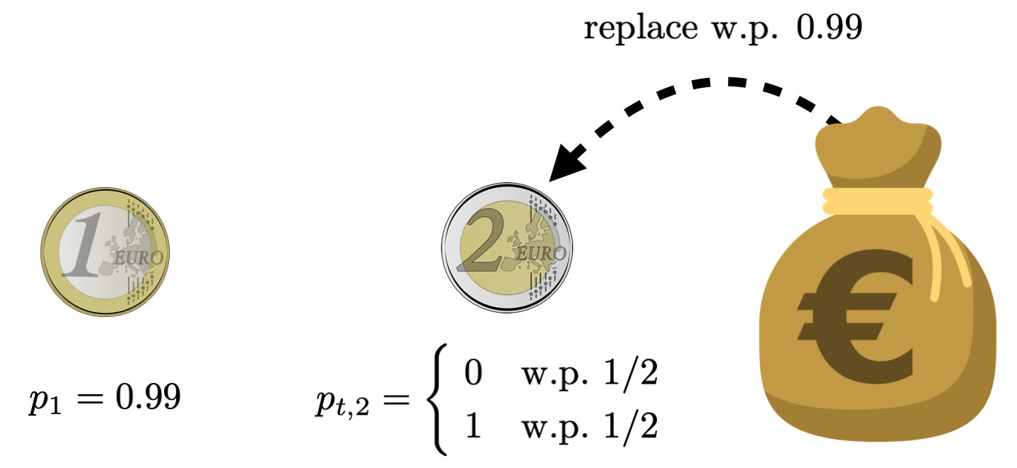
Figure 1: Choosing between two coins: one with bias $p_{1}=0.99$ and the other with bias $p_{t,2}$ of either $1$ or $0$. The second coin is replaced each time with probability $0.99$.

In this environment, selecting the first coin offers payoff of $99$¢ per timestep. Selecting the second coin offers $1 if the coin bias is 1 and $0 otherwise, each with equal probability. After a single toss of the second coin, the bias of the second coin is revealed. However, there is a high probability that the second coin is replaced at the next timestep, and the learned bias becomes irrelevant. Therefore, an optimal agent would be one that only ever tosses the first coin, accumulating payoffs at an expected rate of $99$¢ per timestep, instead of investing to learn the bias of the second coin.

Although TS offers an approach to making such sequential decisions, it turns out that it invests in learning the bias of the second coin, the durability of which is poor, and is thus suboptimal in this environment. Observe that this environment is identified by the coin biases $p_{1}$ and $p_{t,2}$. At each timestep, TS samples from the posterior distribution of the coin biases and selects an action that would maximize the sample. Because the first bias is known, at each timestep $t$, TS takes its sample to be $\hat{p}_{t,1}=p_{1}=0.99$. The second coin, on the other hand, is replaced with high probability at each time, and when it is replaced, the bias becomes $0$ or $1$ with equal probability. So $\hat{p}_{t,2}=1$ with a probability that is at least $0.495$. Maximizing between $\hat{p}_{t,1}$ and $\hat{p}_{t,2}$, TS samples the second coin with a probability that is at least $0.495$. A simple derivation shows that TS accumulates payoffs at an expected rate of at most $75$¢ per timestep, which clearly falls far short of the $99$¢ rate that would be earned by repeatedly tossing the first coin.

3.2 Existing Variants of TS Do Not Fix the Issue

A number of variants of TS have been proposed for the purpose of non-stationary bandit learning, including TS with change-detection (Ghatak,, 2021), dynamic TS (Gupta et al.,, 2011), change-point TS (Mellor and Shapiro,, 2013), discounted TS (Raj and Kalyani,, 2017), sliding-window TS (Trovo et al.,, 2020) and reset-aware TS (Viappiani,, 2013). Instead of maintaining an exact posterior distribution, which can be highly computationally demanding in a non-stationary environment, these algorithms strive to employ various heuristics to approximate the posterior distribution, and also to update this approximation in a tractable manner. Each algorithm, similar to what TS would do, samples from the approximate posterior distribution, and selects an action that optimizes the corresponding expected payoff.

In the coin-tossing environment of Figure 1, each of these algorithms maintains an approximate posterior distribution of the coin biases $p_{1}$ and $p_{t,2}$, samples from this distribution, and selects an action that maximizes the sample. Similar to TS, each agent would sample $\hat{p}_{t,1}=0.99$. Recall that the second coin is replaced with probability $0.99$ at each timestep, and when it is replaced, the bias becomes $0$ or $1$ with equal probability. Consequently, if an agent intelligently uses this coin-replacement information in approximating the posterior distribution of the coin biases, the agent would sample $\hat{p}_{t,2}=1$ with a probability that is at least $0.495$. Maximizing between $\hat{p}_{t,1}$ and $\hat{p}_{t,2}$, the agent would select the second coin with a probability that is at least $0.495$ and deviate from the optimal agent that only ever selects the first coin.

Although not all agents would intelligently use the coin-replacement information in approximating the posterior distribution, readers can verify that each of the aforementioned agents would select the second coin with a positive probability. Therefore, similar to TS, these variants of TS invest in learning the bias of the second coin, and these variants are thus suboptimal in this environment. Since the variants of TS behave and perform similarly to TS, we will focus our attention on TS as a benchmark in the rest of the paper.

3.3 TS Can Perform Very Poorly

Now that we have demonstrated that TS deviates from the optimal strategy in some non-stationary environments, we next characterize how bad TS can perform. The main message here is that TS can perform almost as badly as a worst-performing agent in some non-stationary environments.

Consider a variant of the environment of Figure 1, where the decision at each time is to choose which coin among $K$ coins to toss, where $K$ is greater than $2$. The third through $K$-th coins are independent copies of the second coin. That is, each of these coins is drawn independently from the bag and is replaced independently at each time with probability $0.99$. In addition, with this variant, almost all coins in the bag have bias $0$: suppose that $99\%$ of the coins in the bag have bias $0$, and the rest have bias $1$. Figure 2 illustrates this.

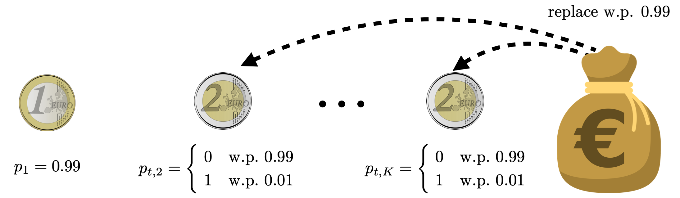
Figure 2: Choosing among $K$ coins: the third through $K$-th coins are independent copies of the second coin.

In such an environment, TS performs almost as badly as the worst-performing agent. To see why, first observe that TS takes $\hat{p}_{t,1}=0.99$ as before. At each time, each of the second through the $K$-th coins is independently replaced with a positive probability $0.99$, and that the bag contains a positive proportion $1\%$ of coins with bias $1$. Therefore, $\hat{p}_{t,k}=1$ with a positive probability, for $k\in\{2,...,K\}$. When $K$ is sufficiently large, by maximizing among $\hat{p}_{t,1},\hat{p}_{t,2},...,\hat{p}_{t,K}$, TS selects one of the second through the $K$-th coins with a sufficiently large probability; the probability converges to $1$ as $K\rightarrow+\infty$. However, tossing any of the second through the $K$-th coins yields an expected payoff at a rate that is close to $0$¢; a simple derivation reveals that this rate is less than $2$¢ per timestep. Therefore, in an environment where $K$ is sufficiently large, TS collects an expected payoff that is at most $2$¢ per timestep, much smaller than the rate of $99$¢ accumulated by an agent that only ever selects the first coin. This gap of $97$¢ in payoffs per timestep is large, considering that the expected payoff per timestep lies in the range $[\$0,\$1]$.

In fact, following a similar argument, we can show that there exists an environment with multiple coins where the performance gap between TS and the optimal agent can be arbitrarily close to $1. In other words, we are able to show that in such an environment, TS accumulates an expected payoff that is arbitrarily close to $\$0$ and that an optimal agent accumulates an expected payoff that is arbitrarily close to $\$1$. Since payoffs in such environments are binary-valued, this indicates that TS performs arbitrarily close to the worst-possible agent for this environment. The above observations will be formalized in Theorem 1 of Section 5.1 using the language of Bernoulli bandits.

4 Definitions

In order to state our theoretical results, we begin by formally defining what a bandit is, what it means to be non-stationary, and several other useful concepts. All random quantities are defined with respect to a probability space $(\Omega,\mathcal{F},\mathbb{P})$.

We first formalize the concept of a bandit. Let $\mathcal{A}$ be a finite set, and $\{R_{t}\}_{t=1}^{+\infty}$ be a stochastic process taking values in $\mathbb{R}^{|\mathcal{A}|}$. A bandit is defined by the tuple $(\{R_{t}\}_{t=1}^{+\infty},\mathcal{A})$, where the two elements correspond to the reward process and the action set, respectively. In particular, for every $t\geq 0$ and $a\in\mathcal{A}$, $R_{t+1,a}$ represents the reward that will be realized if an agent executes action $a$ at timestep $t$. We use $\mathbb{Z}_{+}$ to denote nonnegative integers and $\mathbb{Z}_{++}$ to denote positive integers. We use $R_{1:+\infty}$ as a shorthand for the full reward sequence, and $R_{i:j}$ as a shorthand for the reward sequence $\{R_{t}\}_{t=i}^{j}$.

In order to determine whether a bandit is non-stationary, let us start by proposing a definition of stationary bandits that is consistent with all stationary bandit models in the literature that we are aware of. We say that a bandit is stationary if the reward process, $\{R_{t}\}_{t=1}^{+\infty}$, is exchangeable. That is, the joint distribution of the reward process is invariant under any finite permutation of the time indices. By de Finetti’s theorem, we also obtain an equivalent, and more familiar definition: a bandit is stationary if there exists a distribution $P$ over $\mathbb{R}^{|\mathcal{A}|}$ such that, conditioned on $P$, the rewards are independently and identically distributed according to $P$. We refer to this $P$ as the reward distribution. With the above definition in place, we say a bandit is non-stationary if it is not stationary.

Let $\mathcal{H}$ denote the set of all sequences of a finite number of action-reward pairs. We refer to the elements of $\mathcal{H}$ as histories. A policy is a function that maps a history in $\mathcal{H}$ to a probability distribution over $\mathcal{A}$. So a policy $\pi$ assigns, for each realization of history $h\in\mathcal{H}$, a probability $\pi(a|h)$ of choosing an action $a$ for all $a\in\mathcal{A}$. For any policy $\pi$, we use $A_{t}^{\pi}$ to denote the action selected at time $t$ by an agent that executes policy $\pi$, and $H^{\pi}_{t}$ to denote the history generated at timestep $t$ as an agent executes policy $\pi$. Specifically, we let $H^{\pi}_{0}$ be the empty history, and iteratively define $A_{t}^{\pi}$ and $H_{t+1}^{\pi}$ for all $t\in\mathbb{Z}_{+}$. We let $A_{t}^{\pi}$ be such that $\mathbb{P}(A^{\pi}_{t}\in\cdot|H^{\pi}_{t})=\pi(\cdot|H^{\pi}_{t})$ and that $A_{t}^{\pi}$ is independent of $R_{1:+\infty}$ conditioned on $H_{t}^{\pi}$, and let $H^{\pi}_{t+1}=(A^{\pi}_{0},R_{1,A^{\pi}_{0}},\ldots,A^{\pi}_{t},R_{t,A^{\pi}_{t}})$.

Much of the work presented in this paper studies an agent that executes a specific policy, i.e., PS. Note that when it is clear from the context, we suppress superscripts that indicate this. For example, we use $A_{t}$ for the action selected and $H_{t}$ for the history generated as an agent executes PS.

5 Predictive Sampling

This section introduces the predictive sampling (PS) algorithm.

5.1 Setting a Different Learning Target

We start by introducing a concept that is central to both the design and analysis of PS: learning target. Learning naturally occurs as an agent acquires more information about the rewards process when interacting with a bandit environment. A learning target, $\chi$, is a random variable that formalizes, and further crystallizes, about what the agent aims to learn in this process. For instance, taking $\chi$ to be the mean rewards of different arms, one may cast many existing algorithms for stationary bandits as trying to strike a balance between gaining more information about $\chi$ and maximizing instantaneous rewards (Arumugam and Van Roy, 2021a, ; Arumugam and Van Roy, 2021b, ; Lu et al.,, 2021; Russo and Van Roy,, 2022).

But we can take it a step further, by using the learning target not merely as a device to interpret existing algorithms, but also a design tool to actively shape agent’s exploration behavior. This led us to a crucial insight: by choosing the appropriate learning target in a TS-like algorithm, we can overcome TS’s failure to account for information durability. Specifically, we argue that a promising candidate for the learning target is the sequence of all future rewards, $R_{t+2:\infty}$. Intuitively, one would expect an agent that aims to learn about the entire future reward sequence would naturally have to take into account the durability of the information she gathers in each timestep.

Building on the above insight, the PS algorithm follows naturally from the following two-step procedure: First, we provide a general formulation of TS so as to make the role of the learning target explicit. In particular, we frame TS as an agent who, at each timestep $t$,

1. samples a statistically plausible learning target $\hat{\chi}_{t}$ from its posterior $\mathbb{P}(\chi_{t}\in\cdot|H_{t}^{\pi_{\mathrm{TS}}})$,

2. estimates the conditional mean reward $\hat{\theta}_{t}^{\pi_{\mathrm{TS}}}=\mathbb{E}[R_{t+1}|H_{t}^{\pi_{\mathrm{TS}}},\chi_{t}\leftarrow\hat{\chi}_{t}]$ given the sampled learning target,

3. selects the action that has the highest mean reward estimate.

In the second step, we simply replace the learning target in the above TS procedure with the sequence of all future rewards $R_{t+2:\infty}$, and doing so immediately leads to the PS algorithm.

In other words, PS builds upon TS by changing not how it samples, but what it samples. The most commonly used learning target in TS and its variants is the reward distribution at the current timestep, irrespective of how “quickly” this distribution is about to change. This choice incentivizes an agent to expand valuable resources on learning a piece of information that will quickly lose relevance in a non-stationary environment.

As a concrete piece of evidence, Theorem 1 establishes that a TS agent can suffer near worst-case performance in certain (non-stationary) Bernoulli bandits. Here, we use $\pi_{\text{TS}}$ to denote the policy executed by TS; for any policy $\pi$ and $T\in\mathbb{Z}_{+}$, denote by $\mathrm{Return}(T;\pi)$ the expected cumulative reward collected by an agent that executes $\pi$:

$$\mathrm{Return}(T;\pi)=\sum_{t=0}^{T-1}\mathbb{E}\left[R_{t+1,A_{t}^{\pi}}\right];$$

a Bernoulli bandit is a bandit where the rewards are $\{0,1\}$-valued.

Theorem 1.

For all $\epsilon\in(0,1)$, there exists a Bernoulli bandit $\nu$ and a policy $\pi$ such that under $\nu$,

$$\mathrm{Return}(T;\pi_{\mathrm{TS}})\leq\epsilon T,\text{ and }\mathrm{Return}(T;\pi)\geq(1-\epsilon)T,\quad\mbox{for all $T\in\mathbb{Z}_{++}$.}$$

A proof of this result is provided in Appendix C.

5.2 The Predictive Sampling Algorithm

1 for $t=0,1,\ldots,T-1$ do

2       sample: $\hat{R}^{(t)}_{t+2:\infty}\sim\mathbb{P}(R_{t+2:\infty}\in\cdot|H_{t})$

3       estimate: $\hat{\theta}_{t}=\mathbb{E}[R_{t+1}|H_{t},R_{t+2:\infty}\leftarrow\hat{R}^{(t)}_{t+2:\infty}]$

4       select: $A_{t}\in\operatorname*{arg\,max}_{a\in\mathcal{A}}\hat{\theta}_{t,a}$

5       observe: $R_{t+1,A_{t}}$

Algorithm 1 Predictive sampling (PS)

Figure 3: The predictive sampling algorithm

We now provide a formal description of PS, summarized in Figure 3. At each timestep $t$, PS performs the following steps:

1. samples an infinite sequence of future rewards $\hat{R}_{t+2:\infty}^{(t)}$ from its posterior distribution, $\mathbb{P}(R_{t+2:\infty}\in\cdot|H_{t})$,

2. estimates expected mean rewards by deriving an estimate $\hat{\theta}_{t}$, by “pretending” that $\hat{R}_{t+2:\infty}^{(t)}$ is the sequence of true future rewards $R_{t+2:\infty}$:

   $$\hat{\theta}_{t}=\mathbb{E}[R_{t+1}|H_{t},R_{t+2:\infty}\leftarrow\hat{R}^{(t)}_{t+2:\infty}],$$ (1)

3. selects the action that maximizes $\hat{\theta}_{t,a}$, by setting $A_{t}\in\operatorname*{arg\,max}_{a\in\mathcal{A}}\hat{\theta}_{t,a}$.

In Step 2, the notation $X\leftarrow Y$ denotes a change of measure from that of the random variable $X$ to that of the random variable $Y$: if we let $f(x)=\mathbb{E}[R_{t+1}|H_{t},R_{t+2:\infty}=x]$, then $\hat{\theta}_{t}=f(\hat{R}^{(t)}_{t+2:\infty})$. This notation is formally defined in Appendix B.2.

6 Qualitative Properties of PS

Next, we use some examples to illustrate two salient qualitative properties of PS. First, it reacts to information durability, and benefits from doing so. Second, in stationary environments, it coincides with the behavior of TS, and is therefore expected to perform just as well as TS.

6.1 PS Reacts to Information Durability

Let us use the type of coin-tossing environments in Figures 1 and 2 to illustrate the mechanism through which PS takes information durability into account. First, observe that PS samples the mean reward estimate $\hat{\theta}_{t}$ according to:

$$\mathbb{P}\left(\hat{\theta}_{t}\in\cdot|H_{t}\right)=\mathbb{P}\left(\mathbb{E}[R_{t+1}|H_{t},R_{t+2:\infty}\leftarrow\hat{R}^{(t)}_{t+2:\infty}]\in\cdot|H_{t}\right)=\mathbb{P}\left(\mathbb{E}[R_{t+1}|H_{t},R_{t+2:\infty}]\in\cdot|H_{t}\right),$$

where we have used the fact that the trajectory of future rewards are sampled with respect to the posterior distribution: $\mathbb{P}(\hat{R}^{(t)}_{t+2:\infty}\in\cdot|H_{t})=\mathbb{P}(R_{t+2:\infty}\in\cdot|H_{t})$.

In other words, PS samples the mean reward estimate $\hat{\theta}_{t}$ from the posterior distribution of $\mathbb{E}[R_{t+1}|H_{t},R_{t+2:\infty}]$, conditional on the history $H_{t}$. Let us examine how this distribution changes as a function of the information durability of an action. Consider the example given in Figure 1, where in every timestep the second coin can be replaced with a new coin drawn from the bag with a certain probability, and we will denote this probability of redraw by $q$. Intuitively, the smaller $q$ is, the less likely that the current second coin would be replaced, and therefore the more durable any information about its distribution.

In this example, due to the independence between the biases of the two coins, we see that the mean reward estimate for second coin, $\hat{\theta}_{t,2}$, is drawn from the posterior distribution of $\mathbb{E}[R_{t+1,2}|H_{t},R_{t+2:\infty,2}]$ conditional on the history $H_{t}$. When the redraw probability $q$ is very large, we see that the distribution of $\mathbb{E}[R_{t+1,2}|H_{t},R_{t+2:\infty,2}]$ is relatively insensitive to the realized value of $R_{t+2:\infty,2}$, because there would have likely been a “redraw” shortly after $t$, and therefore the values of future rewards beyond the “redraw” would have little influence on our knowledge about $R_{t+1}$. This further implies that this would induce a relatively small variance in the sampling distribution of $\hat{\theta}_{t,2}$, since multiple values of $R_{t+2:\infty,2}$ can all lead to similar final outcome for $\hat{\theta}_{t,2}$.

On the other hand, when the redraw probability $q$ is small, i.e., when the information associated with the second coin is durable, we see the opposite effect. In this case, $\mathbb{E}[R_{t+1,2}|H_{t},R_{t+2:\infty,2}]$ is much more sensitive to the realization of $R_{t+2:\infty,2}$, beyond just the first few entries, because the agent can more confidently leverage many entries of the future rewards to infer the value of the next reward, $R_{t+1,2}$, knowing that there’s hardly any redrawing occurring between now and then. Consequently, we would expect the sampling distribution for $\hat{\theta}_{t,2}$ to have a larger variance.

In general, all else being equal, increasing the variance of the sampling distribution of the mean reward estimate of an action tends to encourage the exploration of that action. The above analysis therefore suggests that PS naturally tends to favor exploring actions that have higher information durability, a desirable feature.

To illustrate the performance impact from PS’s use of information durability, let us revisit the example in Theorem 1. The next theorem shows that PS excels, and in fact achieves near-optimal performance, in a bandit environment where TS failed. A complete proof is provided in Appendix C.

Theorem 2.

For all $\epsilon\in(0,1)$, under the Bernoulli bandit $\nu$ specified in Theorem 1, we have that

$$\mathrm{Return}(T;\pi_{\mathrm{PS}})\geq(1-\epsilon)T,\quad\mbox{for all $T\in\mathbb{Z}_{++}$.}$$

Finally, we can apply PS to the coin-tossing environments of Figures 1 and 2. It turns out PS executes the optimal policy in both instances. In the two-coin environment of Figure 1, each reward $R_{t}$ corresponds to the payoff, and PS takes the sequence of future payoffs $R_{t+2:\infty}$ to be the learning target. Since the first coin has a known bias of $0.99$, PS takes $\hat{\theta}_{t,1}=0.99$. Recall that the second coin is replaced with probability $0.99$ at each timestep; half of the coins in the bag have bias $0$, and the other half bias $1$. Therefore, the sample $\hat{\theta}_{t,2}$ is close to $0.5$. Consequently, by maximizing between $\hat{p}_{t,1}$ and $\hat{p}_{t,2}$, PS only ever selects the first coin and executes the optimal policy in this environment.

For the $K$-coin environment of Figure 2, PS takes $\hat{\theta}_{t,1}=0.99$ as before. Recall that in this environment, the second coin is again replaced with probability $0.99$ at each timestep, but $99\%$ of the coins in the bag have bias $0$ and $1\%$ have bias $1$. Therefore, the sample $\hat{\theta}_{t,2}$ is close to $0.01$; a simple derivation reveals that $\hat{\theta}_{t,2}\in(0,0.02)$. Recall that each of the third through the $K$-th coins is an independent copy of the second coin. Therefore, $\hat{\theta}_{t,k}\in(0,0.02)$ for all $k\in\{2,...,K\}$. By maximizing among $\hat{\theta}_{t,1},\hat{\theta}_{t,2},...,\hat{\theta}_{t,K}$, PS only ever selects the first coin and executes the optimal policy in this environment. Thus, a PS agent accumulates expected payoffs at a rate of $99$¢ per timestep. This is much higher than the rate of at most $2$¢ of the TS agent described in Section 3.

6.2 PS Coincides with TS in Stationary Bandits

We show here that in a stationary bandit, PS executes the same policy as TS, if the latter uses the reward distribution as the learning target; recall that the notion of a policy is defined in Section 4. This is a very useful property because we can thus be assured that PS is guaranteed to succeed also in the type of stationary bandits where TS thrives.

Proposition 1.

In any stationary bandit where the reward distribution is $P$, a PS agent and a TS agent that takes $\chi_{t}=P$ for all $t\in\mathbb{Z}_{+}$ execute the same policy.

The proof is given in Appendix D and leverages the fact that in a stationary bandit, the reward distribution is equivalent to PS’s learning target; more precisely, the reward distribution $P$ and PS’s learning target of the sequence of future rewards $R_{t+2:\infty}$ are equally informative in predicting the immediate reward $R_{t+1}$.

7 Regret Analyses

The previous sections have presented several desirable properties of PS and showcased their performance implications in some examples. The goal of this section is to provide general theoretical guarantees on the performance of PS for a much wider range of environments.

To do so, we will first introduce a notion of regret for non-stationary bandits. We then establish a theoretical framework for information-theoretic regret analyses, which generalizes that developed by Russo and Van Roy, (2014) for stationary bandits. Critical to the framework is a new information ratio and the concept of predictive information. We establish a regret bound that applies to any agent. We specialize the bound to PS and then further to non-stationary Bernoulli bandits. These bounds suggest that PS performs well across a range of such bandits.

7.1 Performance and Regret

Regret is a widely used metric in the bandit learning literature that measures the difference between the rewards collected by an oracle and that by an agent. While traditionally the oracle is one who knows and chooses the optimal action, this choice does not extend to a non-stationary environment when the reward distributions themselves evolve over time. The first definition of regret that we will consider involves an oracle that sees the entirety of all realizations of past rewards from all actions, $R_{1:t}$, and selects the action at each timestep to maximize the expected reward $\mathbb{E}[R_{t+1,a}|R_{1:t}]$.

Definition 1 (Hindsight Regret).

For all policies $\pi$ and $T\in\mathbb{Z}_{+}$, the hindsight regret associated with a policy $\pi$ over $T$ timesteps is

$$\mathrm{Regret}_{\mathrm{H}}(T;\pi)=\sum_{t=0}^{T-1}\mathbb{E}\left[R_{t+1,*}-R_{t+1,A_{t}^{\pi}}\right],$$ (2)

where $R_{t+1,*}=\max_{a\in\mathcal{A}}\mathbb{E}[R_{t+1,a}|R_{1:t}]$.

Because a real agent cannot observe the rewards of the actions that she did not choose in a given timestep, the aforementioned oracle is ensured to outperform any agent. This fact is formalized in the following result, which indicates that the hindsight regret is always non-negative; the proof is given in Appendix E.

Proposition 2.

For all policies $\pi$ and $T\in\mathbb{Z}_{+}$,

$$\sum_{t=0}^{T-1}\mathbb{E}\left[R_{t+1,*}\right]\geq\sum_{t=0}^{T-1}\mathbb{E}\left[R_{t+1,A_{t}^{\pi}}\right].$$

Because it can be difficult to directly analyze the hindsight regret in general bandit environments, we will also introduce a second regret definition, which will serve as a more tractable proxy for hindsight regret within the family of non-stationary bandits that we will focus on. Instead of an oracle who sees all past rewards, we consider an oracle that instead has access to the realizations of all future reward realizations, and subsequently chooses the action that maximizes the conditional mean reward $\mathbb{E}[R_{t+1,a}|R_{t+2:\infty}]$.

Definition 2 (Foresight Regret).

For all policies $\pi$ and $T\in\mathbb{Z}_{+}$, the foresight regret associated with a policy $\pi$ over $T$ timesteps is

$$\mathrm{Regret}_{\mathrm{F}}(T;\pi)=\sum_{t=0}^{T-1}\mathbb{E}\left[R_{t+1,\overline{*}}-R_{t+1,A_{t}^{\pi}}\right],$$ (3)

where $R_{t+1,\overline{*}}=\max_{a\in\mathcal{A}}\mathbb{E}[R_{t+1,a}|R_{t+2:\infty}]$.

The foresight regret has an advantage in tractability. Because our main aim in this paper is to characterize the performance of PS, which takes simulated future trajectories as a crucial input, foresight regret is more amenable to analysis because the oracle therein also uses future reward trajectories to drive actions. Furthermore, we will show in the subsequent section that, within a family of non-stationary bandits with a reversibility structure, foresight regret is always no smaller than hindsight regret, thus making it useful as a tool to upper-bound the latter.

Another benefit of foresight regret is that it generalizes the conventional notion of regret used in stationary bandit learning literature (Lai and Robbins,, 1985; Neu et al.,, 2022). To see why, observe that in a stationary bandit, an oracle that sees all future rewards will simply pick the action with the largest mean at all timesteps. As a result, the upper bounds we derive with foresight regret can then by compared to known bounds on conventional regret when the bandit is stationary.

7.2 Reversible Bandits

The majority of our theoretical results will focus on the performance of an agent in a class of non-stationary bandits which we will refer to as reversible bandits. They are defined as follows:

Definition 3 (Reversible Bandit).

A bandit is reversible if the reward process $\{R_{t}\}_{t=1}^{+\infty}$ is reversible in the following sense: for all $T\in\mathbb{Z}_{++}$, $\{R_{t}\}_{t=1}^{T}$ and $\{R_{T+1-t}\}_{t=1}^{T}$ have the same joint distribution.

Reversible bandits encompass a wide range of bandit environments. All stationary bandits are reversible, so are all non-stationary bandits discussed in this paper, including the modulated Bernoulli bandits, AR(1) bandits, and AR(1) logistic bandits. There are certainly non-stationary bandits that are not reversible, whose analyses will be outside the scope of this paper but we believe can be an interesting direction for future work.

The following result shows that in a reversible bandit, the hindsight regret (Definition 1) is always bounded from above by the foresight regret (Definition 2); the proof is provided in Appendix F. As a consequence, we will be focusing on characterizing the foresight regret of an agent in the remainder of the paper, with the understanding that any upper bound will also apply to the hindsight regret when the bandit is reversible.

Proposition 3.

Suppose the bandit is reversible. For all policies $\pi$ and $T\in\mathbb{Z}_{+}$,

$$\mathrm{Regret}_{\mathrm{H}}(T;\pi)\leq{\mathrm{Regret}}_{\mathrm{F}}(T;\pi).$$

7.3 Predictive Information and a New Information Ratio

As our primary analytical framework, we will be using a variant of the information-theoretic regret analysis developed in the stationary bandit learning literature. This analysis was first used by (Russo and Van Roy,, 2016) for analyzing TS and subsequently extended to many other settings (Bubeck et al.,, 2015; Lattimore and Szepesvári,, 2019; Lu et al.,, 2021; Neu et al.,, 2022). The key idea is to bound the regret in terms of a certain information ratio, $\Gamma$, defined to be the ratio between a function of the immediate regret and the information gain about a learning target. The logic is that a “good” agent who optimally balances between information acquisition and reward maximization ought to have a relatively small information ratio, and vice versa. While proven extremely versatile in analyzing various stationary bandit learning agents, the aforementioned framework does not apply to non-stationary environments. One of the key obstacles is that the information ratio originally defined for stationary bandits do not generalize easily.

To overcome this challenge, we introduce in this paper a new information ratio that is better suited to our regret analysis for non-stationary bandits. The first change is that we now measure immediate regret with respect to the benchmark $R_{t+1,\overline{*}}$ as per Definition 2, instead of the reward associated with the optimal action as in stationary bandits. The second, and more important, change is that we now measure information gain with respect to a new learning target, the sequence of future rewards, $R_{t+2:\infty}$, in contrast to using the current reward distribution as the learning target in stationary bandits. Formally, we define the information ratio associated with policy $\pi$ at timestep $t$ be

$$\Gamma_{t}^{\pi}=\frac{\mathbb{E}\left[R_{t+1,\overline{*}}-R_{t+1,A_{t}^{\pi}}\right]^{2}}{\mathbb{I}\left(R_{t+2:\infty};A_{t}^{\pi},R_{t+1,A_{t}^{\pi}}|H_{t}\right)}.$$ (4)

This information ratio measures how an agent trades off between a single-timestep regret and information about $R_{t+2:\infty}$. Since much of the paper studies PS, we simplify the notation in this case and use $\Gamma_{t}$ to denote the information ratio associated with PS.

As mentioned earlier, the foresight regret coincides with the conventional regret definition in stationary bandits. Similarly, it is easy to show that the information gain defined here also coincides with one for stationary bandits (cf. Neu et al., (2022)).

Next, we introduce the notion of predictive information. It represents the new information that is being injected to the environment during each timestep, due to non-stationarity. Specifically, for all $t$, we define the incremental predictive information at time $t$ as the mutual information between the next reward $R_{t+1}$ and the sequence of all future rewards $R_{t+2:\infty}$, conditional on $R_{1:t}$. The definition is formalized below.

Definition 4 (Incremental Predictive Information).

For all $t\in\mathbb{Z}_{+}$, the incremental predictive information at timestep $t$ is

$$\Delta_{t}=\mathbb{I}(R_{t+2:\infty};R_{t+1}|R_{1:t}).$$

Intuitively, $\Delta_{t}$ measures the incremental information one can learn about future rewards $R_{t+2:\infty}$ by observing current reward $R_{t+1}$, after having already observed all past rewards $R_{1:t}$. If the environment is highly stationary, then as $t$ increases, there is little additional information gained from observing the current reward, because most of the information about future rewards are already contained in the past rewards $R_{1:t}$. On the other hand, when the environment is highly non-stationary, historical data plays a less important role, and observing the most recent reward $R_{t+1}$ can be extremely helpful in predicting future rewards no matter how large $t$ is. In summary, one would expect that the predictive information $\Delta_{t}$ to decay as $t$ increases in a stationary environment, but to remain relatively large in a non-stationary one. This behavior is consistent with what we would expect from a good metric to quantify information.

Finally, we refer to the cumulative sum of incremental predictive information, $\sum_{t^{\prime}=0}^{t-1}\Delta_{t^{\prime}}$, as the cumulative predictive information at time $t$, representing the total new uncertainty that has been injected into the environment thus far. The cumulative predictive information will play a crucial role in our analysis, and deriving an upper bound on it often allows us to further upper-bounding the regret itself.

7.4 Regret Bounds for General Agents

We are now ready to present our regret analysis. We begin with Theorem 3, which establishes a general upper bound on foresight regret that applies to any agent in any bandit. In particular, the bound is expressed in terms of the sum of the information ratios $\sum_{t=0}^{T-1}\Gamma_{t}^{\pi}$ and the cumulative predictive information $\sum_{t=0}^{T-1}\Delta_{t}$.

Theorem 3.

For all policies $\pi$ and $T\in\mathbb{Z}_{+}$,

$${\mathrm{Regret}}_{\mathrm{F}}(T;\pi)\leq\sqrt{\sum_{t=0}^{T-1}\Gamma_{t}^{\pi}\sum_{t=0}^{T-1}\Delta_{t}}.$$

The proof is provided in Appendix G. The proof leverages the fact that when an agent incurs regret, it must acquire some amount of information that is relevant for predicting future rewards $R_{t+2:\infty}$. Therefore, we can upper-bound the cumulative regret by how the agent trades off between immediate regret and such information, which is measured by the sum of information ratios $\sum_{t=0}^{T-1}\Gamma_{t}^{\pi}$, and the cumulative predictive information $\sum_{t=0}^{T-1}\Delta_{t}$, which upper-bounds the total information that an agent acquires to predict future rewards.

We will subsequently use the general regret bound of Theorem 3 by separately bounding the two constituent terms, $\sum_{t=0}^{T-1}\Gamma_{t}^{\pi}$ and $\sum_{t=0}^{T-1}\Delta_{t}$, respectively. The former depends on the choice of the agent or algorithm, while the latter is a function only of the underlying bandit environment. Because the cumulative predictive information is agent-independent, we will begin with it and first introduce Lemma 1. The lemma provides an elegant approach towards bounding the cumulative predictive information in any bandit; the proof is provided in Appendix H.

Lemma 1.

Let $\{S_{t}\}_{t=1}^{+\infty}$ be a Markov process such that, for all $t\in\mathbb{Z}_{+}$, $S_{t+1:\infty}\perp R_{1:t}|S_{t}$ and $R_{t+2:\infty}\perp R_{t+1}|S_{t+2},R_{1:t}$. For all $T\in\mathbb{Z}_{+}$, the cumulative predictive information satisfies

$$\sum_{t=0}^{T-1}\Delta_{t}\leq\mathbb{I}(S_{2};S_{1})+\sum_{t=1}^{T-1}\mathbb{I}(S_{t+2};S_{t+1}|S_{t})$$

The random variable $S_{t}$ in the above lemma can be thought of as the hidden state of the bandit at timestep $t$. By suitably constructing $\{S_{t}\}_{t=1}^{+\infty}$, we can apply this lemma to bound predictive information in any bandit. In particular, this can be achieved by letting $S_{t}=R_{1:t}$ for all $t\in\mathbb{Z}_{++}$. For some bandits, there is a better choice of $\{S_{t}\}_{t=1}^{+\infty}$ with which we can derive sharper bounds or more interpretable bounds when applying the lemma.

It is worth noting that, by combining Lemma 1 and Theorem 3, and specializing the resulting bound to stationary bandits, we can recover existing regret bounds for stationary bandits. See Appendix I for this result.

7.5 Regret Bounds for PS

We now turn our attention to using the general regret bound of Theorem 3 to obtain sharper regret bounds for PS in various non-stationary bandits.

We begin by obtaining an upper bound on the information ratio $\Gamma_{t}=\Gamma_{t}^{\pi_{\mathrm{PS}}}$ associated with PS, expressed in terms of the number of actions and the variance of the rewards. The proof of the following result is provided in Appendix J.

Lemma 2.

If for all $t\in\mathbb{Z}_{+}$ and $a\in\mathcal{A}$, $\mathbb{P}(R_{t+1,a}\in\cdot|H_{t})$ is almost surely $\sigma_{\text{SG}}$-sub-Gaussian, then for all $t\in\mathbb{Z}_{+}$, the information ratio associated with PS satisfies

$$\Gamma_{t}\leq 2|\mathcal{A}|\sigma_{\mathrm{SG}}^{2}.$$

The following theorem follows directly from combining Theorem 3 and Lemma 2. It establishes a regret bound for PS in terms of the cumulative predictive information.

Theorem 4.

If for all $t\in\mathbb{Z}_{+}$ and $a\in\mathcal{A}$, $\mathbb{P}(R_{t+1,a}\in\cdot|H_{t})$ is almost surely $\sigma_{\text{SG}}$-sub-Gaussian, then for all $T\in\mathbb{Z}_{+}$, the regret of PS satisfies

$${\mathrm{Regret}}_{\mathrm{F}}(T)\leq\sqrt{2|\mathcal{A}|\sigma_{\mathrm{SG}}^{2}T\sum_{t=0}^{T-1}\Delta_{t}}.$$

Finally, using Lemma 1 to better characterize the cumulative predictive information, we obtain the following refinement.

Corollary 1.

Let $\{S_{t}\}_{t=1}^{+\infty}$ be a Markov process such that, for all $t\in\mathbb{Z}_{+}$, $R_{t}\perp R_{1:t-1,t+1:\infty},S_{1:t-1,t+1:\infty}|S_{t}$. If for all $t\in\mathbb{Z}_{+}$ and $a\in\mathcal{A}$, $\mathbb{P}(R_{t+1,a}\in\cdot|H_{t})$ is almost surely $\sigma_{\text{SG}}$-sub-Gaussian, then for all $T\in\mathbb{Z}_{+}$, the regret of PS satisfies

$${\mathrm{Regret}}_{\mathrm{F}}(T)\leq\sqrt{2|\mathcal{A}|\sigma_{\mathrm{SG}}^{2}T\left[\mathbb{I}(S_{2};S_{1})+\sum_{t=1}^{T-1}\mathbb{I}(S_{t+2};S_{t+1}|S_{t})\right]}.$$

Note that specializing the bound of PS in Corollary 1 to stationary bandits, we can recover existing regret bounds for TS in stationary bandits. See Appendix I for this result.

7.6 Regret Bounds in Modulated Bernoulli Bandits

Building on the results from the previous section, we now focus on a specific model of non-stationary, reversible bandits that will enable us to derive a sharper and more interpretable regret bound.

A majority of the existing literature on non-stationary bandit learning focuses on Bernoulli bandits, and for this reason we will focus our analysis on this family as well. Below, we consider a family of non-stationary Bernoulli bandits that generalizes an abrupt switching model introduced by Mellor and Shapiro, (2013). It is easy to verify that bandits in family are reversible, and also encompass both coin-tossing environments introduced in Section 3.

Example 1 (Modulated Bernoulli Bandit).

Consider a Bernoulli bandit with independent actions. For all $a\in\mathcal{A}$, let $\{\theta_{t,a}\}_{t=0}^{+\infty}$ be a sequence of random variables. We refer to $\theta_{t,a}$ as the mean reward associated with action $a$ at timestep $t$; conditioning on $\theta_{t,a}$, the reward $R_{t+1,a}\sim$ Bernoulli($\theta_{t,a}$), independent of the rewards and mean rewards associated with other timesteps or actions. Each mean reward sequence $\{\theta_{t,a}\}_{t=0}^{+\infty}$ transitions according to

$$\theta_{t+1,a}=\begin{cases}\sim\mathbb{P}(\theta_{0,a}\in\cdot),&\ \text{with probability $q_{a}$},\\ \theta_{t,a},&\ \text{otherwise},\end{cases}$$

where $q_{a}\in[0,1]$ is deterministic and known. At each timestep, the mean reward $\theta_{t,a}$ can be thought of as “redrawn” from its initial distribution independently with probability $q_{a}$.

We are now ready to present the main result of this section: an upper bound on the regret of PS in a modulated Bernoulli bandit. The detailed derivation is presented in Appendix K. It leverages Corollary 1 by carefully constructing a sequence $\{S_{t}\}_{t=1}^{+\infty}$ where we set $S_{t}=\theta_{t-1}$ for all $t\in\mathbb{Z}_{+}$.

Theorem 5.

In a modulated Bernoulli bandit, the regret of PS satisfies

$${\mathrm{Regret}}_{\mathrm{F}}(T)\leq\sqrt{\frac{1}{2}|\mathcal{A}|T\left\{\sum_{a\in\mathcal{A}}(1-q_{a})\mathbb{H}(\theta_{0,a})+(T-1)\sum_{a\in\mathcal{A}}\left[2\mathbb{H}(q_{a})+q_{a}(1-q_{a})\mathbb{H}(\theta_{0,a})\right]\right\}}.$$

A first observation is that the above regret upper bound scales linearly in horizon, $T$. Interestingly, this scaling matches the next regret lower bound that we present, suggesting that the linear scaling in $T$ in our upper bound is tight. A proof is provided in Appendix L.

Theorem 6.

There exists a modulated Bernoulli bandit and a constant $C\in\mathbb{R}_{++}$ such that, for all policies $\pi$ and $T\in\mathbb{Z}_{+}$, the foresight regret satisfies

$${\mathrm{Regret}}_{\mathrm{F}}(T;\pi)\geq CT.$$

Together, Theorems 5 and 6 serve as encouraging evidence that PS performs competitively in modulated Bernoulli bandits.

Furthermore, we can use Theorem 5 to investigate how the performance of PS depends on various key parameters of the environment. Crucially, the bound exhibits a graceful dependence on $q_{a}$, the probability that a coin is redrawn in each timestep. On one hand, when $q_{a}=0$ for all $a$, i.e., when the environment is stationary, the bound becomes ${\mathrm{Regret}}_{\mathrm{F}}(T)=\sqrt{\frac{1}{2}|\mathcal{A}|T\mathbb{H}(\theta_{0})}$, which recovers a current best known regret bound for TS (Neu et al.,, 2022). On the other hand, as the $q_{a}$’s approach $1$, the regret bound approaches $0$, suggesting that PS performs well. Recall that this is a setting where the coins are redrawn frequently, and therefore the optimal policy is to always choose the coin whose bias has the highest mean with respect to its initial distribution. As we illustrated earlier, PS correctly follows this optimal behavior in the specific examples outlined in Section 3, and our regret bound further confirms that it continues to excel even in more general bandit environments.

8 Efficient Implementations and Experiments

While the PS procedure is very easy to state, deriving the conditional probability distribution and subsequently sampling from the distribution can be computationally challenging. To address this, this section introduces efficient procedures to execute PS in some bandits and useful techniques to execute an approximation of the algorithm in others. In particular, we develop an efficient implementation of PS in a class of Gaussian bandits. We also design efficient procedures to execute an approximation of PS in a class of logistic bandits. To examine the advantage of PS over TS, we conduct experiments in the aforementioned class of Gaussian bandits and logistic bandits. The results suggest that PS consistently outperforms TS over time in environments with varying information durability. Additionally, we compare PS with other representative non-stationary bandit learning algorithms and show that PS consistently outperforms them.

8.1 PS in AR(1) Bandits

We consider a class of Gaussian bandits, which we refer to as AR(1) bandits, where each bandit is determined by a sequence $\{\alpha_{t,a}\}_{t\in\mathbb{Z}+}$ that independently transitions according to a first-order autoregressive (AR(1)) process. We study AR(1) bandits because AR(1) processes have been commonly used to model non-stationary processes in fields such as nature and economics, and moreover, other non-stationary bandits of similar fomulation have been studied by Gupta et al., (2011); Kuhn et al., (2015); Kuhn and Nazarathy, (2015); Slivkins and Upfal, (2008).

Example 2 (AR(1) Bandit).

In an AR(1) bandit, each reward $R_{t+1,a}$ is distributed according to a Gaussian distribution with a random mean $\theta_{t,a}=\alpha_{t,a}$ and a deterministic variance $\sigma_{a}^{2}$. Each realized reward can be interpreted as a sum $R_{t+1,a}=\theta_{t,a}+Z_{t+1,a}$, where $Z_{t+1,a}$ is independent zero-mean noise with deterministic variance $\sigma_{a}^{2}$. The variable $\alpha_{t,a}$ changes over time, evolving according to

$$\alpha_{t+1,a}=(1-\gamma_{a})c_{a}+\gamma_{a}\alpha_{t,a}+W_{t+1,a},$$

for each action $a\in\mathcal{A}$. The coefficients $c_{a}$ and $\gamma_{a}$ are deterministic, and each takes value in $\mathbb{R}$ and $[0,1]$, respectively; $W_{t+1,a}$ is independent zero-mean Gaussian noise with deterministic variance $\delta_{a}^{2}$, where $\delta_{a}\in\mathbb{R}_{+}$. When $\gamma_{a}=1$, we require that $\delta_{a}=0$ and that $\theta_{0,a}$ is Gaussian. We assume that the sequence $\{\alpha_{t,a}\}_{t\in\mathbb{Z}_{+}}$ is in steady-state: when $\gamma_{a}<1$, this steady-state distribution is $\mathcal{N}(c_{a},\delta_{a}^{2}/(1-\gamma_{a}^{2}))$.

Note that the formulation of AR(1) bandits accommodates stationary Gaussian bandits with independent actions as a special case. Specifically, if we let $\gamma_{a}=1$ and $\delta_{a}=0$ for all $a\in\mathcal{A}$, then $\alpha_{t+1,a}=\alpha_{0,a}$ for all $t\in\mathbb{Z}_{+}$ and $a\in\mathcal{A}$. Since $\alpha_{0,a}$ is a Gaussian random variable for all $a\in\mathcal{A}$, we recover a stationary Gaussian bandit with independent actions. We can model any stationary Gaussian bandit with independent actions using an AR(1) bandit with $\gamma_{a}=1$ and $\delta_{a}=0$ for $a\in\mathcal{A}$ and suitably-chosen $\alpha_{0,a}$ for each $a\in\mathcal{A}$.

When interacting with an AR(1) bandit, we assume that an agent knows a priori $c_{a}$, $\gamma_{a}$, $\delta_{a}$, $q_{a}$, $\mathbb{P}(\theta_{0,a}\in\cdot)$, and $\sigma_{a}$ for all $a\in\mathcal{A}$. In fact, this assumption is not necessary: an agent can learn these parameters. In other words, an agent is able to estimate these parameters quite accurately after a finite number of timesteps that is large enough. Since we are interested in the performance of an agent in the regime $T\rightarrow+\infty$, the performance of the agent in the learning phase of the first finite number of timesteps is irrelevant. Therefore, we can focus on investigating the performance of an agent after it learns these parameters. Without loss of generality, we can assume that the parameters are known to the agent a priori. Similar assumptions appear in (Slivkins and Upfal,, 2008) and (Mellor and Shapiro,, 2013) and techniques to estimate such parameters based on historical data have been discussed in (Wilson et al.,, 2010; Turner et al.,, 2009).

8.1.1 Efficient Implementation of PS

While we are interested in developing efficient procedures to execute PS in an AR(1) bandit, as a stepping stone, we first focus on implementing TS that takes $\chi_{t}=\theta_{t}$ to be its learning target. In an AR(1) bandit, TS samples at each timestep $\hat{\theta}_{t}^{\pi_{\mathrm{TS}}}$ from $\mathbb{P}(\theta_{t}\in\cdot|H_{t}^{\pi_{\mathrm{TS}}})$, and selects an action that maximizes $\hat{\theta}_{t,a}^{\pi_{\mathrm{TS}}}$. Recall that in an AR(1) bandit, $\mathbb{P}(\theta_{0}\in\cdot)$ is Gaussian. When action $a$ is selected at timestep $t$, the agent observes $R_{t+1,a}\sim\mathcal{N}(\theta_{t,a},\sigma_{a}^{2})$, where $\sigma_{a}$ is deterministic and known. Therefore, $\mathbb{P}(\theta_{t}\in\cdot|H_{t}^{\pi_{\mathrm{TS}}})$ is Gaussian. We use $\mu_{t}^{\pi_{\mathrm{TS}}}$ and $\Sigma_{t}^{\pi_{\mathrm{TS}}}$ to denote the mean and covariance of it; they can be derived using Kalman filter. Algorithm 3 provides an implementation of TS in an AR(1) bandit; for the sake of simplicity, we drop the superscript $\pi_{\mathrm{TS}}$.

For PS, we develop an efficient implementation of it based on the following observation from Section 6.1: Steps 2 and 3 of Algorithm 1 are equivalent to sampling $\hat{\theta}_{t}$ from

$$\mathbb{P}(\mathbb{E}[R_{t+1}|H_{t},R_{t+2:\infty}]\in\cdot|H_{t})=\mathbb{P}(\mathbb{E}[\theta_{t}|H_{t},R_{t+2:\infty}]\in\cdot|H_{t}).$$ (5)

Since the rewards are jointly Gaussian, the above distribution is Gaussian. We use $\tilde{\mu}_{t}$ and $\tilde{\Sigma}_{t}$ to denote its mean and covariance. We present Algorithm 2, which provides an implementation of PS in an AR(1) bandit.

1 for $t=0,1,\ldots,T-1$ do

2       sample: $\hat{\theta}_{t}\sim\mathcal{N}(\tilde{\mu}_{t},\tilde{\Sigma}_{t})$

3       execute: $A_{t}\in\operatorname*{arg\,max}_{a\in\mathcal{A}}\hat{\theta}_{t,a}$

4       observe: $R_{t+1,A_{t}}$

5       update: $\tilde{\mu}_{t+1}\leftarrow\mathbb{E}[\theta_{t+1}|H_{t+1}]$

6               $\tilde{\Sigma}_{t+1}\leftarrow\mathbb{V}(\mathbb{E}[\theta_{t+1}|H_{t},R_{t+2:\infty}]|H_{t+1})$

Algorithm 2 PS in an AR(1) bandit

1 for $t=0,1,\ldots,T-1$ do

2       sample: $\hat{\theta}_{t}\sim\mathcal{N}(\mu_{t},\Sigma_{t})$

3       execute: $A_{t}\in\operatorname*{arg\,max}_{a\in\mathcal{A}}\hat{\theta}_{t,a}$

4       observe: $R_{t+1,A_{t}}$

5       update: $\mu_{t+1}\!\leftarrow\!\mathbb{E}[\theta_{t+1}|H_{t+1}]$

6           $\Sigma_{t+1}\!\leftarrow\!\mathbb{V}(\theta_{t+1}|H_{t+1})$

Algorithm 3 TS in an AR(1) bandit

Step 5 of Algorithm 2 is the most challenging to implement, and we now show how it can be done. Observe that the distribution $\mathbb{P}(\theta_{t}\in\cdot|H_{t})$ is Gaussian. We use $\mu_{t}$ and $\Sigma_{t}$ to denote the mean and covariance of it, and they can be derived analytically using Kalman filter. The values of $\tilde{\mu}_{t}$ and $\tilde{\Sigma}_{t}$ can be derived using $\mu_{t}$ and $\Sigma_{t}$. Specifically, because both $\Sigma_{t}$ and $\tilde{\Sigma}_{t}$ are diagonal, we use $\sigma_{t,a}^{2}$ and $\tilde{\sigma}_{t,a}^{2}$ to denote each entry along their diagonals, respectively. The following result establishes the exact analytical forms for $\tilde{\mu}_{t,a}$ and $\tilde{\sigma}^{2}_{t,a}$, as function of $\mu_{t,a}$ and $\sigma^{2}_{t,a}$. The proof is presented in Appendix M.

Proposition 4.

In an AR(1) bandit, for all $t\in\mathbb{Z}_{+}$ and $a\in\mathcal{A}$, conditioned on $H_{t}$, $\hat{\theta}_{t,a}$ is Gaussian with mean and variance

$$\ \tilde{\mu}_{t,a}=\mu_{t,a}\text{ and }\tilde{\sigma}_{t,a}^{2}=\frac{\gamma_{a}^{2}\sigma_{t,a}^{4}}{\gamma_{a}^{2}\sigma_{t,a}^{2}+x_{a}^{*}},$$

where $x_{a}^{*}=\frac{1}{2}\left(\delta_{a}^{2}+\sigma_{a}^{2}-\gamma_{a}^{2}\sigma_{a}^{2}+\sqrt{(\delta_{a}^{2}+\sigma_{a}^{2}-\gamma_{a}^{2}\sigma_{a}^{2})^{2}+4\gamma_{a}^{2}\delta_{a}^{2}\sigma_{a}^{2}}\right)$.

8.1.2 Experiments

We next conduct experiments in a sequence of AR(1) bandits where the actions are associated with varying degrees of information durability and compare the performance of PS against that of TS. Note that in an AR(1) bandit, $\gamma_{a}$ captures the durability of information associated with action $a\in\mathcal{A}$, with $\gamma_{a}=1$ indicating that the information durability is infinite and $\gamma_{a}=0$ indicating that the information durability is zero. Then we conduct experiments in bandits with varying $\gamma_{a}$ for $a\in\mathcal{A}$.

In particular, we let $\mathcal{A}=\{1,2\}$, the stationary distribution of each arm’s mean reward be $\mathcal{N}(0,1)$, and $\gamma_{1},\gamma_{2}\in\{0.1,0.3,0.5,0.7,0.9\}$. This defines a range of two-armed AR(1) bandits where each mean reward distribution is standard normal, and $\gamma_{1}$ and $\gamma_{2}$ each varies in a discrete grid in $(0,1)$. By symmetry in actions, we examine bandits where $\gamma_{1}\in\{0.1,0.3,0.5\}$ and $\gamma_{2}\in\{0.1,0.3,0.5,0.7,0.9\}$, respectively.

PS Outperforms TS Across Bandits

Figure 4(a) plots the average reward collected by PS and that collected by TS over a long duration of $T=1000$ timesteps, which serve as good approximations to the long-run average rewards collected by the two agents. The plot shows that PS consistently outperforms TS, regardless of information durability associated with the actions. This provides additional evidence, complementing our theoretical analyses and examples, to support that PS has advantage over TS in non-stationary bandits.

The plot also suggests that both PS and TS perform better in bandits with a larger value of $\gamma_{1}$ or $\gamma_{2}$. This is consistent with our intuition that any given agent tends to perform better in bandits with better information durability because they can put the information learned so far to better use for longer periods of time.

PS Outperforms TS Across Time

Now that we have examined the long-run performance of PS, we next investigate if PS sacrifices its short-term performance for long-term benefits. In particular, we focus on one example of the aforementioned AR(1) bandits, with $\gamma_{1}=0.1$ and $\gamma_{2}=0.9$ and plot the mean rewards across a number of timesteps. Figure 4(b) plots the average reward collected by PS and that collected by TS over $t\in\{1,2,...,200\}$ timesteps, with the error bars representing 95% confidence intervals. We observe that PS consistently outperforms TS across time.

The phenomenon that PS outperforms TS across time can be observed beyond this example. We present additional plots in Appendix O that illustrate this. The plots suggest that the phenomenon is persistent across a diverse set of AR(1) bandit instances.

(a) The average rewards collected over $T=1000$ timesteps in the environments where $\gamma_{1}\in\{0.1,0.3,0.5\}$, $\gamma_{2}\in\{0.1,0.3,0.5,0.7,0.9\}$

(b) An example: the average rewards collected over $t\in\{1,...,200\}$ timesteps in an environment where $\gamma_{1}=0.1$, $\gamma_{2}=0.9$

Figure 4: The average rewards collected by PS and that collected by TS in AR(1) bandits

8.2 AR(1) Logistic Bandits

We next consider a class of bandits which we refer to as AR(1) logistic bandits. Just like the AR(1) bandits, the reward distributions of these bandits are governed by a sequence $\{\alpha_{t}\}_{t\in\mathbb{Z}_{+}}$ that evolves according to an AR(1) process, but in this case the rewards will be Bernoulli. This class extends bandits modulated by AR(1) processes to logistic bandits. We study AR(1) logistic bandits because it serves as a first step towards implementing PS in contextual bandits and further in practical problems.

Example 3 (AR(1) Logistic Bandit).

In an AR(1) logistic bandit, each reward $R_{t+1,a}$ is Bernoulli distributed with mean $\frac{\exp(\alpha_{t}^{\top}\phi_{a})}{1+\exp(\alpha_{t}^{\top}\phi_{a})}$, where $\alpha_{t}\in\mathbb{R}^{d}$ is unknown with a known dimension $d\in\mathbb{Z}_{++}$ and $\phi_{a}\in\mathbb{R}^{d}$ denotes a known feature vector associated with action $a\in\mathcal{A}$. The variable $\alpha_{t,a}$ is defined exactly as in Example 2, transitioning following an AR(1) process.

Similarly, the formulation of AR(1) logistic bandits accommodates stationary logistic bandits as a special case. In particular, following a similar argument to that of AR(1) bandits, we can model any stationary logistic bandit using an AR(1) logistic bandit with $\gamma_{a}=1$ and $\delta_{a}=0$ for $a\in\mathcal{A}$ and suitably-chosen $\alpha_{0,a}$ for each $a\in\mathcal{A}$. As was the case with the AR(1) bandits, we assume that an agent knows a priori $c_{a}$, $\gamma_{a}$, $\delta_{a}$, $q_{a}$, $\mathbb{P}(\theta_{0,a}\in\cdot)$, and $\sigma_{a}$ for all $a\in\mathcal{A}$.

8.2.1 Approximate PS in AR(1) Logistic Bandits

We next discuss techniques to approximate PS and apply those techniques to AR(1) logistic bandits to develop efficient implementations.

Incremental Laplace Approximation And Approximate TS

We first introduce a technique that is useful in developing tractable procedues to approximate PS in AR(1) logistic bandits. For better exposition, we will first demonstrate this technique in the context of implementing an approximation of TS in AR(1) logistic bandits. In an AR(1) logistic bandit, a natural learning target is $\alpha_{t}$. We thus focus on TS that takes $\alpha_{t}$ as its learning target. At each timestep, TS samples $\hat{\alpha}_{t}^{\pi_{\mathrm{TS}}}$ from the posterior of $\alpha_{t}$, and selects an action that maximizes the expected reward conditioned on the sample.

Because deriving the posterior of $\alpha_{t}$ is usually intractable, we can instead apply Laplace approximation (Laplace,, 1986). That is, we approximate the posterior using a Gaussian distribution centered at the maximum a posteriori (MAP) of $\alpha_{t}$, with a variance that is equal to the inverse of the Hessian of the log-posterior. This is a standard practice and has been popular with stationary logistic bandits and contextual bandits (Chapelle and Li,, 2011).

However, when the environment is non-stationary, applying the method to approximate the posterior of $\alpha_{t}$ can be computationally onerous. To address this, we propose what we call incremental Laplace approximation—the practice of approximating the posterior distribution incrementally at each timestep using Laplace approximation. Incremental Laplace approximation is comparable with the standard Laplace approximation in stationary logistic bandits, but can be efficiently carried out in non-stationary ones.

1 for $t=0,1,\ldots,T-1$ do

2       sample: $\hat{\alpha}_{t}$ from $\mathcal{N}(\mu_{t},\Sigma_{t})$

3       estimate: $\hat{\theta}_{t}=\phi^{\top}\hat{\alpha}_{t}$

4       select: $A_{t}\in\operatorname*{arg\,max}_{a\in\mathcal{A}}\hat{\theta}_{t,a}$

5       observe: $R_{t+1,A_{t}}$

6       derive: $\mu_{t+1}\leftarrow\min_{\alpha}\left\{\frac{1}{2}(\alpha-\mu_{t})^{\top}\Sigma_{t}^{-1}(\alpha-\mu_{t})-R_{t+1,A_{t}}\phi_{A_{t}}\alpha+\log\left(1+\exp\left(\phi_{A_{t}}\alpha\right)\right)\right\}$, and $\Sigma_{t+1}\leftarrow\left\{\Sigma_{t}+{\exp(\phi_{A_{t}}\mu_{t+1})}{\left[1+\exp\left(\phi_{A_{t}}\mu_{t+1}\right)\right]^{-2}}\phi_{A_{t}}^{\top}\phi_{A_{t}}\right\}^{-1}$

7       update: $\mu_{t+1}\leftarrow A\mu_{t+1}\text{ and }\Sigma_{t+1}\leftarrow A\Sigma_{t+1}A^{\top}+V$

8      

Algorithm 4 Approximate TS in an AR(1) logistic bandit

Applying incremental Laplace approximation, we develop an efficient implementation of an approximation of TS in an AR(1) logistic bandit. It is detailed in Algorithm 4; for the sake of simplicity, we drop the superscript $\pi_{\mathrm{TS}}$. Step 6 carries out incremental Laplace approximation. In Step 7, $A$ denotes a diagonal matrix with $\gamma_{a}$ at its $a$-th position along its diagonal, and $V$ a diagonal matrix with $\delta_{a}^{2}$ at its $a$-th position along its diagonal.

Finite-sample Approximation

Another technique that is useful in constructing computationally tractable approximations of PS is to sample a finite number of rewards instead of an infinite sequence of rewards in executing the algorithm. In Algorithm 1, this corresponds to changing Steps 2 and 3 to:

1. sample $\hat{R}^{(t)}_{t+2:t+n+1}\sim\mathbb{P}(R_{t+2:t+n+1}\in\cdot|H_{t})$,

2. estimate $\hat{\theta}_{t}=\mathbb{E}[R_{t+1}|H_{t},R_{t+2:t+n+1}\leftarrow\hat{R}^{(t)}_{t+2:t+n+1}]$.

The new Steps 2 and 3 are equivalent to sampling $\hat{\theta}_{t}$ from the distribution $\mathbb{P}(\mathbb{E}[R_{t+1}|H_{t},R_{t+2:t+n+1}]\in\cdot|H_{t})$. To see why, first observe that for all $t\in\mathbb{Z}_{+}$, $\mathbb{P}(\hat{R}^{(t)}_{t+2:t+n+1}\in\cdot|H_{t})=\mathbb{P}(R_{t+2:t+n+1}\in\cdot|H_{t})$. Therefore, for all $t\in\mathbb{Z}_{+}$,

$$\mathbb{P}(\hat{\theta}_{t}\in\cdot|H_{t})=\mathbb{P}(\mathbb{E}[R_{t+1}|H_{t},R_{t+2:t+n+1}\leftarrow\hat{R}^{(t)}_{t+2:t+n+1}]\in\cdot|H_{t})=\mathbb{P}(\mathbb{E}[R_{t+1}|H_{t},R_{t+2:t+n+1}]\in\cdot|H_{t}).$$

Gaussian Imagination

If the sampling distribution $\mathbb{P}(\mathbb{E}[R_{t+1}|H_{t},R_{t+2:t+n+1}]\in\cdot|H_{t})$ of an approximation of PS have closed-form solutions, then we can design efficient procedures to execute the algorithm. Regardless of whether this is computationally tractable, an agent can approximate this distribution by pretending that the rewards are Gaussian. This practice is called Gaussian imagination (Liu et al.,, 2022). Specifically, an agent can construct imaginary Gaussian rewards $\tilde{R}_{t+1}$ for all $t\in\mathbb{Z}_{+}$; the imaginary rewards live in the agent’s imagination and are designed to approximate real rewards. The agent then estimates $\mathbb{P}(\mathbb{E}[R_{t+1}|H_{t},R_{t+2:t+n+1}]\in\cdot|H_{t})$ using $\mathbb{P}(\mathbb{E}[\tilde{R}_{t+1}|H_{t},\tilde{R}_{t+2:t+n+1}]\in\cdot|H_{t})$.

Approximate PS

We next apply finite-sampling approximation, Gaussian imagination, and incremental Laplace approximation to approximate PS in AR(1) logistic bandits. Specifically, this approximation algorithm, which we refer to as approximate PS, samples $\hat{\theta}_{t}$ from the an approximate posterior of $\mathbb{E}[\tilde{R}_{t+1}|H_{t},\tilde{R}_{t+2:t+n+1}]$, and selects an action that maximizes $\hat{\theta}_{t,a}$. In applying Gaussian imagination, we let $\tilde{R}_{t+1}\sim\mathcal{N}\left(\frac{1}{2}\mathbf{1}+\frac{1}{4}\phi^{\top}\alpha_{t},\frac{1}{16}I\right),$ where $\mathbf{1}$ is an all-one vector and $\phi$ is the matrix whose $a$-th column is $\phi_{a}$. With this definition of $\tilde{R}_{t+1}$, $\mathbb{E}[\tilde{R}_{t+1}|H_{t},\tilde{R}_{t+2:t+n+1}]=\frac{1}{2}\mathbf{1}+\frac{1}{4}\phi^{\top}\mathbb{E}[\alpha_{t}|H_{t},\tilde{R}_{t+2:t+n+1}]$. Therefore, equivalently, approximate PS can sample $\hat{\alpha}_{t}$ from an approximate posterior distribution of $\mathbb{E}[\alpha_{t}|H_{t},\tilde{R}_{t+2:t+n+1}]$ and select an action that maximizes $\phi^{\top}\hat{\alpha}_{t,a}$.

Applying incremental Laplace approximation, we construct the approximate posterior using a Gaussian distribution $\mathcal{N}(\mu^{\prime}_{t},\Sigma^{\prime}_{t})$. More precisely, we first approximate the posterior of $\alpha_{t}$ using a Gaussian distribution $\mathcal{N}(\mu_{t},\Sigma_{t})$ according to incremental Laplace approximation, and then derive $\mu_{t}^{\prime}$ and $\Sigma_{t}^{\prime}$ based on $\mu_{t}$ and $\Sigma_{t}$. Detailed steps about this derivation are provided in Appendix N.

The implementation of approximate PS in an AR(1) logistic bandit is presented in Algorithm 5. It is worth highlighting that the only difference between approximate PS and approximate TS in an AR(1) logistic bandit is that between the sampling distribution of $\hat{\alpha}_{t}$ and $\hat{\alpha}_{t}^{\pi_{\mathrm{TS}}}$. In Algorithm 5, Step 6 again carries out incremental Laplace approximation to incrementally derive $\mu_{t}$ and $\Sigma_{t}$. As we have discussed, Appendix N presents details on how we can derive $\mu^{\prime}_{t}$ and $\Sigma^{\prime}_{t}$ based on $\mu_{t}$ and $\Sigma_{t}$.

1 for $t=0,1,\ldots,T-1$ do

2       sample: $\hat{\alpha}_{t}$ from $\mathcal{N}(\mu^{\prime}_{t},\Sigma^{\prime}_{t})$

3       estimate: $\hat{\theta}_{t}=\phi^{\top}\hat{\alpha}_{t}$

4       select: $A_{t}\in\operatorname*{arg\,max}_{a\in\mathcal{A}}\hat{\theta}_{t,a}$

5       observe: $R_{t+1,A_{t}}$

6       derive: $\mu_{t+1}\leftarrow\min_{\alpha}\left\{\frac{1}{2}(\alpha-\mu_{t})^{\top}\Sigma_{t}^{-1}(\alpha-\mu_{t})-R_{t+1,A_{t}}\phi_{A_{t}}\alpha+\log\left(1+\exp\left(\phi_{A_{t}}\alpha\right)\right)\right\}$, and $\Sigma_{t+1}\leftarrow\left\{\Sigma_{t}^{-1}+{\exp(\phi_{A_{t}}\mu_{t+1})}{\left[1+\exp\left(\phi_{A_{t}}\mu_{t+1}\right)\right]^{-2}}\phi_{A_{t}}^{\top}\phi_{A_{t}}\right\}^{-1}$

7       update: $\mu_{t+1}\leftarrow A\mu_{t+1},\Sigma_{t+1}\leftarrow A\Sigma_{t+1}A^{\top}+V$, and update $\mu^{\prime}_{t}$ and $\Sigma^{\prime}_{t}$ according to incremental Laplace approximation

Algorithm 5 Approximate PS in an AR(1) logistic bandit

8.2.2 Experiments

We now conduct experiments to examine the performance of approximate PS. Since the experiment design and the analyses are similar to that concerning PS in Section 8.1.2, some repetition is expected but is kept to a minimum. In particular, we compare approximate PS with approximate TS in a sequence of AR(1) logistic bandits where $\alpha_{t,1}$ is associated with information of varying durability. We also examine both the case where the actions are independent and the case where the actions are dependent. Specifically, we let $\mathcal{A}=\{1,2,3\}$, the stationary distribution of each $\alpha_{t,k}$ be $\mathcal{N}(0,1)$, and $\gamma=[\gamma_{1},0.9,0.9]$, where $\gamma_{1}\in\{0.1,0.9,0.99\}$. In addition, we let $\phi\in\{\phi^{\text{ind}},\phi^{\mathrm{dep}}\}$, where

$$\phi^{\mathrm{ind}}=\begin{bmatrix}1&0&0\\ 0&1&0\\ 0&0&1\end{bmatrix}\text{ and }\phi^{\mathrm{dep}}=\begin{bmatrix}0.9&0.1&0\\ 0&0.9&0.1\\ 0.1&0&0.9\end{bmatrix}.$$

Note that $\gamma_{1}$ determines the durability of the information associated with $\alpha_{t,1}$; the feature matrix $\phi$ determines weather the actions are independent, with $\phi^{\mathrm{ind}}$ indicating that the actions are independent, and $\phi^{\mathrm{dep}}$ indicating that the actions are dependent. Therefore, the set of parameters define a range of three-armed AR(1) logistic bandits with varying durability of information associated with $\alpha_{t,1}$, and accommodates both the case where the actions are independent and the case where the actions are dependent.

Approximate PS Outperforms Approximate TS Across Bandits

Figure 5(a) plots the average rewards collected by approximate PS and that by approximate TS over a long duration of $T=1000$ timesteps, to study the long-run performance of the algorithms. The plot shows that approximate PS consistently outperforms approximate TS. These results support the efficacy of approximate PS and the usefulness of the techniques we introduced to approximate PS.

Approximate PS Outperforms Approximate TS Across Time

Similar to how we investigate PS, we also investigate if approximate PS sacrifices its short-term performance for long-term benefits. We focus on an example in the aforementioned AR(1) logistic bandits, with $\gamma_{1}=0.1$ and $\phi=\phi^{\mathrm{ind}}$. Figure 5(b) plots the average reward collected by approximate PS and that collected by approximate TS over $t\in\{1,2,...,200\}$ timesteps, with the error bars representing $95\%$ confidence intervals. The results suggest that approximate PS outperforms approximate TS across time.

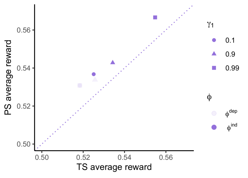
(a) The average rewards collected over $T=1000$ timesteps in the environments where $\phi\in\{\phi^{\mathrm{ind}},\phi^{\mathrm{dep}}\}$, $\gamma_{1}\in\{0.1,0.9,0.99\}$

(b) An example: the average rewards collected over $t\in\{1,...,200\}$ timesteps in an environment where $\gamma_{1}=0.1$, $\phi=\phi^{\text{ind}}$

Figure 5: The average rewards collected by approximate PS and that collected by approximate TS in AR(1) logistic bandits

8.3 Comparison with Other Algorithms

This section presents experiments we conduct to compare PS with non-stationary bandit learning algorithms beyond TS and its variants.

8.3.1 Algorithms and Environments

A large set of algorithms (Besbes et al.,, 2019; Besson and Kaufmann,, 2019; Cheung et al.,, 2019; Garivier and Moulines,, 2008; Ghatak,, 2021; Gupta et al.,, 2011; Hartland et al.,, 2006; Kocsis and Szepesvári,, 2006; Mellor and Shapiro,, 2013; Raj and Kalyani,, 2017; Trovo et al.,, 2020; Viappiani,, 2013) designed for non-stationary bandit learning focuses on making better inference about current mean reward; given what is inferred, these algorithms usually apply action-selection schemes that are designed for stationary bandits, such as TS, upper-confidence-bound methods (Lai and Robbins,, 1985), and the exponential-weight algorithms (Auer et al.,, 2002; Freund and Schapire,, 1997). In this sense, one can think of these algorithms as taking the current mean reward as the learning target; in particular, to make it more concrete, when applied to the coin-tossing environments of Section 3, this learning target corresponds to the coin biases. Therefore, these algorithms, with TS and its existing variants as special cases, do not intelligently account for the information durability when selecting actions, and we believe that PS has advantages over these algorithms in non-stationary bandit learning.

Algorithms

We conduct experiments with a representative subset of these non-stationary bandit learning algorithms. Since there are three popular heuristics on making inference on current mean reward, i.e., using a fixed-length sliding-window, weighing data by recency, and periodic restarts, we choose one algorithm focusing on each of the three heuristics. In addition, we take a naive TS agent, who executes TS while pretending that the bandit is stationary, as a baseline. Below we briefly describe each of the four representative algorithms with which we conduct experiments.

• Rexp3 (Besbes et al.,, 2019) uses Exp3 as a action-selection subroutine and restarts it periodically.

• Discounted UCB (Garivier and Moulines,, 2008) uses UCB1 as a subroutine and discounts the effect of past rewards on estimating current reward distribution by weighing past data according to recency.

• Sliding-window UCB (Garivier and Moulines,, 2008) maintains a sliding-window of fixed size and uses UCB1 as a subroutine.

• Naive TS pretends that the bandit is stationary and proceeds with inference.

Environments

We next introduce the class of bandits in which we conduct the experiments and any additional details in implementing the algorithms. Because past work that introduced Rexp3, discounted UCB, and sliding-window UCB conduct experiments in bandits where the rewards are bounded, we restrict our attention to such bandits. In addition, to analyze how the information durability affect the performance of the agents, we also would like to conduct experiments in bandits where the information durabilities are determined by particular environment parameters, the adjustments of which adjust the information durabilities. To accommodate both needs, we design a set of bandits that differ from the AR(1) bandits only in that the rewards are truncated to $[0,1]$.

In implementating the algorithms, the parameters of Rexp3 are chosen according to Theorem 2 of (Besbes et al.,, 2019), where the “variation budget” is assumed to be known in advance for each simulation; the parameters in discounted UCB and sliding-window UCB are chosen according to Remark 3 and Remark 9 of (Garivier and Moulines,, 2008), respectively, where “the number of breakpoints” is assumed to be known in advance. In implementing PS, the agent pretends that the rewards are not truncated.

8.3.2 Experiments

We conduct two sets of experiments. The first one in a bandit where $\mathcal{A}=\{1,2\}$, $c_{1}=c_{2}=0.5$, $\gamma_{1}=\gamma_{2}=0.85$, $\delta_{a}=0.15(1-\gamma_{a}^{2})$ for $a\in\mathcal{A}$, and $\sigma_{1}=\sigma_{2}=0.1$. This describes a bandit with two symmetric actions. Figure 6(a) plots the average frequency of selecting action $2$ over $t\in\{1,2,...,2000\}$ timesteps. As expected, since the actions are symmetric, all agents select each action half of the time in the long run. Figure 6(b) plots the average reward collected by the agents over $t\in\{1,2,...,2000\}$ timesteps, with the error bars representing 95% confidence intervals. The results suggest that a majority of the non-stationary bandit learning algorithms outperforms native TS, and PS outperforms all others. This is consistent with our theoretical results that PS selects actions intelligently accounting for information durability, and as such has advantages in non-stationary bandits.

(a) Frequencies of selecting action $2$

(b) Average rewards collected by each agent

Figure 6: PS and representative algorithms in a bandit with two actions, where $c_{1}=c_{2}=0.5$, $\gamma_{1}=\gamma_{2}=0.85$, $\delta_{a}=0.15(1-\gamma_{a}^{2})$ for $a\in\mathcal{A}$, and $\sigma_{1}=\sigma_{2}=0.1$

We conduct our second set of experiments in a bandit where $\mathcal{A}=\{1,2\}$, $c_{1}=0.65,c_{2}=0.55$, $\gamma_{1}=0.1,\gamma_{2}=0.99$, $\delta_{a}=0.15(1-\gamma_{a}^{2})$ for $a\in\mathcal{A}$, and $\sigma_{1}=\sigma_{2}=0.1$. This corresponds to a bandit with two asymmetric actions: action $1$ is associated with a mean reward that has a larger mean $c_{1}=0.65$ and changes very quickly, as suggested by $\gamma_{1}=0.1$; action $2$ is associated with a mean reward that has a smaller mean $c_{2}=0.55$ and changes very slowly, as suggested by $\gamma_{2}=0.99$.

Figure 7(a) plots the average action selection frequency. As expected, we observe that the average frequency of selecting action $2$ by naive TS converges to zero, because $c_{2}<c_{1}$. As for PS, since $\gamma_{1}$ is small, PS’s sampling distribution for the mean reward associated with action $1$ is very much concentrated at $c_{1}$. Since $c_{1}$ is much larger than $c_{2}$ and that $\delta_{a}$ isn’t too large, PS selects action $2$ with a small probability. In other words, PS is aware that action $1$ is associated with information that is less durable and as such explores action $1$ less. Note that this does not necessarily imply that PS selects action $1$ with a smaller probability—in fact, since $c_{1}>c_{2}$, this implies that PS selects action $1$ with a larger probability and action $2$ with a smaller probability. In contrast, the rest of the algorithms do not account for the poor information durability associated with action $1$, and as such selects action $2$ more than PS does. This is evident from Figure 7(a).

Figure 7(b) plots the average rewards accumulated by the agents, with the error bars representing 95% confidence intervals. The results reveal that PS accumulates more rewards compared with other agents. This suggests that PS has advantages in non-stationary bandits because it intelligently account for the durability of information and as a result selects action $2$ less compared to other algorithms.

(a) Frequencies of selecting action $2$

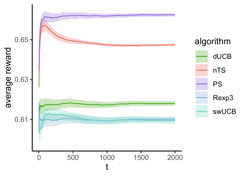
(b) Average rewards collected by each agent

Figure 7: PS and representative algorithms in a bandit with two actions, where $c_{1}=0.65,c_{2}=0.55$, $\gamma_{1}=0.1,\gamma_{2}=0.99$, $\delta_{a}=0.15(1-\gamma_{a}^{2})$ for $a\in\mathcal{A}$, and $\sigma_{1}=\sigma_{2}=0.1$

9 Concluding Remarks

This paper demonstrates that TS and its variants that were proposed in the literature often do not perform well in non-stationary bandits, because they fail to intelligently account for the durability of information when selecting actions. To address this, we propose PS, an algorithm that can be viewed as a version of TS that takes the sequence of future rewards as the learning target. We develop efficient procedures to execute PS in AR(1) bandits and a practical approximation of it in AR(1) logistic bandits. We demonstrate the efficacy of PS through coin-tossing examples, regret bounds, and numerical experiments.

At a high level, our paper illustrates how we can improve an existing algorithm (TS) to arrive at a new algorithm (PS) that is better suited for non-stationary bandits, by changing its learning target. As discussed in Sections 2 and 8.3, a number of other existing algorithms also do not account for the durability of information when selecting actions. Therefore, an interesting future direction would be to ask whether we could modify these other algorithms by taking the sequence of future rewards to be the learning target, and perhaps achieve even more drastic performance improvements in non-stationary environments.

While the sequence of future rewards has proven to be an effective learning target for our purpose, the story needs not stop there. It would be interesting to investigate whether there are other, potentially more powerful learning targets. For example, by suitably defining the “optimal action” at each timestep, we may alternatively take the sequence of future optimal actions as the learning target. It remains an open question how these alternative learning targets would perform in non-stationary environments, how to design algorithms with efficient implementations with respect to these learning targets, and how the current framework needs to adapt for their analyses.

Acknowledgement

This work is partially supported by Army Research Office (ARO) grant W911NF2010055, the MS&E Fellowship Fund of Stanford University, and Statistics for Improving Insights, Models, and Decisions Grant of Meta.

Appendix A Probabilistic Framework

Probability theory emerges from an intuitive set of axioms, and this paper builds on that foundation. Statements and arguments we present have precise meaning within the framework of probability theory. However, we often leave out measure-theoretic formalities for the sake of readability. It should be easy for a mathematically-oriented reader to fill in these gaps.

We will define all random quantities with respect to a probability space $(\Omega,\mathcal{F},\mathbb{P})$. The probability of an event $F\in\mathcal{F}$ is denoted by $\mathbb{P}(F)$. For any events $F,G\in\mathcal{F}$ with $\mathbb{P}(G)>0$, the probability of $F$ conditioned on $G$ is denoted by $\mathbb{P}(F|G)$.

A random variable is a function with the set of outcomes $\Omega$ as its domain. For any random variable $Z$, $\mathbb{P}(Z\in\mathcal{Z})$ denotes the probability of the event that $Z$ lies within a set $\mathcal{Z}$. The probability $\mathbb{P}(F|Z=z)$ is of the event $F$ conditioned on the event $Z=z$. When $Z$ takes values in $\mathbb{R}$ and has a density $p_{Z}$, though $\mathbb{P}(Z=z)=0$ for all $z$, conditional probabilities $\mathbb{P}(F|Z=z)$ are well-defined and denoted by $\mathbb{P}(F|Z=z)$. For fixed $F$, this is a function of $z$. We denote the value, evaluated at $z=Z$, by $\mathbb{P}(F|Z)$, which is itself a random variable. Even when $\mathbb{P}(F|Z=z)$ is ill-defined for some $z$, $\mathbb{P}(F|Z)$ is well-defined because problematic events occur with zero probability.

For each possible realization $z$, the probability $\mathbb{P}(Z=z)$ that $Z=z$ is a function of $z$. We denote the value of this function evaluated at $Z$ by $\mathbb{P}(Z)$. Note that $\mathbb{P}(Z)$ is itself a random variable because it depends on $Z$. For random variables $Y$ and $Z$ and possible realizations $y$ and $z$, the probability $\mathbb{P}(Y=y|Z=z)$ that $Y=y$ conditioned on $Z=z$ is a function of $(y,z)$. Evaluating this function at $(Y,Z)$ yields a random variable, which we denote by $\mathbb{P}(Y|Z)$.

We denote independence of random variables $X$ and $Y$ by $X\perp Y$ and conditional independence, conditioned on another random variable $Z$, by $X\perp Y|Z$.

Appendix B Concepts, Notations, and Relations

We review some standard information-theoretic concepts and associated notations, and introduce a change-of-measure notation in this section.

B.1 Information-Theoretic Concepts, Notations, and Relations

A central concept is the entropy $\mathbb{H}(X)$, which quantifies the information content or, equivalently, the uncertainty of a random variable $X$. For a random variable $X$ that takes values in a countable set $\mathcal{X}$, we will define the entropy to be $\mathbb{H}(X)=-\mathbb{E}[\ln\mathbb{P}(X)]$, with a convention that $0\ln 0=0$. Note that we are defining entropy here using the natural rather than binary logarithm. As such, our notion of entropy can be interpreted as the expected number of nats—as opposed to bits—required to identify $X$. The realized conditional entropy $\mathbb{H}(X|Y=y)$ quantifies the uncertainty remaining after observing $Y=y$. If $Y$ takes on values in a countable set $\mathcal{Y}$ then $\mathbb{H}(X|Y=y)=-\mathbb{E}[\ln\mathbb{P}(X|Y)|Y=y]$. This can be viewed as a function $f(y)$ of $y$, and we write the random variable $f(Y)$ as $\mathbb{H}(X|Y=Y)$. The conditional entropy $\mathbb{H}(X|Y)$ is its expectation $\mathbb{H}(X|Y)=\mathbb{E}[\mathbb{H}(X|Y=Y)]$.

The mutual information $\mathbb{I}(X;Y)=\mathbb{H}(X)-\mathbb{H}(X|Y)$ quantifies information common to random variables $X$ and $Y$, or equivalently, the information about $Y$ required to identify $X$. If $Z$ is a random variable taking on values in a countable set $\mathcal{Z}$ then the realized conditional mutual information $\mathbb{I}(X;Y|Z=z)$ quantifies remaining common information after observing $Z=z$, defined by $\mathbb{I}(X;Y|Z=z)=\mathbb{H}(X|Z=z)-\mathbb{H}(X|Y,Z=z)$. The conditional mutual information $\mathbb{I}(X;Y|Z)$ is its expectation $\mathbb{I}(X;Y|Z)=\mathbb{E}[\mathbb{I}(X;Y|Z=Z)]$.

For random variables $X$ and $Y$ taking on values in (possibly uncountable) sets $\mathcal{X}$ and $\mathcal{Y}$, mutual information is defined by $\mathbb{I}(X;Y)=\sup_{f\in\mathcal{F}_{\text{finite}},g\in\mathcal{G}_{\text{finite}}}\mathbb{I}(f(X);g(Y))$, where $\mathcal{F}_{\text{finite}}$ and $\mathcal{G}_{\text{finite}}$ are the sets of functions mapping $\mathcal{X}$ and $\mathcal{Y}$ to finite ranges. Specializing to the case where $\mathcal{X}$ and $\mathcal{Y}$ are countable recovers the previous definition. The generalized notion of entropy is then given by $\mathbb{H}(X)=\mathbb{I}(X;X)$. Conditional counterparts to mutual information and entropy can be defined in a manner similar to the countable case.

We will make use of KL-divergence as measures of difference between distributions. We denote KL-divergence by

$$\mathbf{d}_{\mathrm{KL}}(P\|P^{\prime})=\int P(dx)\ln\frac{dP}{dP^{\prime}}(x).$$

Gibbs’ inequality asserts that $\mathbf{d}_{\mathrm{KL}}(P\|P^{\prime})\geq 0$, with equality if and only if $P$ and $P^{\prime}$ agree almost everywhere with respect to $P$.

The following result is established by Theorem 5.2.1 of (Gray,, 2011).

Lemma 3 (Variantal Form of the KL-Divergence).

For any probability distribution $P$ and real-valued random variable $X$, both defined with respect to a measureable space $(\Omega^{\prime},\mathbb{F}^{\prime})$, let $\mathbb{E}_{P}[X]=\int_{x\in\Re}xP(dx)$. For probability distributions $P$ and $P^{\prime}$ on a measureable space $(\Omega^{\prime},\mathbb{F}^{\prime})$ such that $P$ is absolutely continuous with respect to $P^{\prime}$,

$$\mathbf{d}_{\mathrm{KL}}(P\|P^{\prime})=\sup_{X}(\mathbb{E}_{P}[X]-\ln\mathbb{E}_{P^{\prime}}[\exp(X)]),$$ (6)

where the supremum is taken over real-valued random variables on $(\Omega^{\prime},\mathbb{F}^{\prime})$ for which $\mathbb{E}_{Q}[\exp(X)]<\infty$.

Mutual information and KL-divergence are intimately related. For any probability measure $P(\cdot)=\mathbb{P}((X,Y)\in\cdot)$ over a product space $\mathcal{X}\times\mathcal{Y}$ and probability measure $P^{\prime}$ generated via a product of marginals $P^{\prime}(dx\times dy)=P(dx)P(dy)$, mutual information can be written in terms of KL-divergence:

$$\mathbb{I}(X;Y)=\mathbf{d}_{\mathrm{KL}}(P\|P^{\prime}).$$ (7)

Further, the following lemma presents an alternative representation of mutual information.

Lemma 4 (KL-Divergence Representation of Mutual Information).

For any random variables $X$ and $Y$,

$$\mathbb{I}(X;Y)=\mathbb{E}[\mathbf{d}_{\mathrm{KL}}(\mathbb{P}(Y\in\cdot|X)\|\mathbb{P}(Y\in\cdot))].$$ (8)

In other words, the mutual information between $X$ and $Y$ is the KL-divergence between the distribution of $Y$ with and without conditioning on $X$.

Mutual information satisfies the chain rule and the data processing inequality.

Lemma 5 (Chain Rule for Mutual Information).

$$\mathbb{I}(X_{1},X_{2},...,X_{n};Y)=\sum_{i=1}^{n}\mathbb{I}(X_{i};Y|X_{1},X_{2},...,X_{i-1}).$$

Lemma 6 (Data Processing Inequality for Mutual Information).

If $X$ and $Z$ are independent conditioned on $Y$, then

$$\mathbb{I}(X;Y)\geq\mathbb{I}(X;Z).$$

The following lemma presents one useful property of mutual information.

Lemma 7.

Let $A$, $B$, and $C$ be three random variables. If $A\perp C|B$ then

$$\mathbb{I}(A;B|C)\leq\mathbb{I}(A;B).$$

Proof.

We prove for the case where $B$ has finite entropy. For the case where $B$ has infinite entropy, we use differential entropy instead of entropy in the analysis.

$$\mathbb{I}(A;B|C)= \ \mathbb{H}(A|C)-\mathbb{H}(A|B,C)$$

$$= \ \mathbb{H}(A|C)-\mathbb{H}(A|B)$$

$$\leq \ \mathbb{H}(A)-\mathbb{H}(A|B)$$

$$= \ \mathbb{I}(A;B).$$

∎

B.2 Change-of-Measure Notation

To characterize PS, let us define a change-of-measure notation. Consider random variables $X$ and $Y$ and a conditional probability $\mathbb{P}(Y\in\cdot|X=x)$ for all $x$ in the image of $X$. Let $f(x)\equiv\mathbb{P}(Y\in\cdot|X=x)$ and $g(x)\equiv\mathbb{E}[Y|X=x]$, for all $x$ in the image of $X$. Given a random variable $Z$ with the same image as $X$, $f(Z)$ and $g(Z)$ are random variables. We use the notation $\mathbb{P}(Y\in\cdot|X\leftarrow Z)$ for $f(Z)$ and $\mathbb{E}[Y|X\leftarrow Z]$ for $g(Z)$. Note that we use the symbol $\leftarrow$ to distinguish a change of measure from conditioning on an event: in general,

$$\mathbb{P}\left(Y\in\cdot|X\leftarrow Z\right)\neq\mathbb{P}(Y\in\cdot|X=Z),$$

because the former represents a change of measure from $X$ to $Z$, whereas the latter represents the conditional distribution conditioning on the event $\{\omega:X=Z\}$. Similarly, in general, $\mathbb{E}\left[Y|X\leftarrow Z\right]\neq\mathbb{E}[Y|X=Z]$, and we need the former to represent a change of measure.

Appendix C How Much Can PS Improve Over TS: Proof of Theorems 1 and 2

See 1 See 2

Proof.

Consider a modulated Bernoulli bandit (see Example 1) with $K$ arms. Arm $1$ has a deterministic mean of $p_{1}=1-\epsilon$, which does not change over time. Each of arm $2$ through $K$’s mean reward takes value $0$ with probability $\beta$ and $1$ with probability $1-\beta$. The probability of transition for each of arm $2$ through $K$ is $q$.

A PS agent estimates $\hat{\theta}_{t}$ at each timestep $t\in\mathbb{Z}_{+}$. Note that $\hat{\theta}_{t,1}=p_{1}$. For all $a\in\{2,...,K\}$,

$$\mathbb{E}\left[R_{t+1,a}|H_{t},R_{t+2:\infty}\right]=\mathbb{P}\left(\theta_{t,a}=1|H_{t},R_{t+2:\infty}\right)\leq 1-q^{2}\beta\ \text{a.s.}$$

This implies that for all timestep $t\in\mathbb{Z}_{+}$ and $a\in\{2,...,K\}$, $\hat{\theta}_{t,a}\leq 1-q^{2}\beta$ a.s.

When $q$ and $\beta$ are sufficiently large, for $a\in\{2,...,K\}$, $\hat{\theta}_{t,a}\leq 1-q^{2}\beta\leq 1-\epsilon=p_{1}=\hat{\theta}_{t,1}$, and a PS agent selects action $1$ with probability one and collects cumulative reward

$$\mathrm{Return}(T;\pi_{\mathrm{PS}})=p_{1}T=(1-\epsilon)T.$$

A TS agent estimates $\hat{\theta}_{t}^{\pi_{\mathrm{TS}}}$ at each timestep $t\in\mathbb{Z}_{+}$. Note that $\hat{\theta}_{t,1}^{\pi_{\mathrm{TS}}}=p_{1}\in(0,1)$. So a TS agent selects action $1$ at each timestep $t\in\mathbb{Z}_{+}$ with probability

$$\mathbb{P}\left(\max_{a\in\{2,...,K\}}\hat{\theta}_{t,a}^{\pi_{\mathrm{TS}}}<\hat{\theta}^{{\pi}_{\mathrm{TS}}}_{t,1}\bigg{|}H_{t}^{\pi_{\mathrm{TS}}}\right)=\prod_{a=2}^{K}\mathbb{P}\left(\hat{\theta}_{t,a}^{\pi_{\mathrm{TS}}}=0\Big{|}H_{t}^{\pi_{\mathrm{TS}}}\right)\leq\left(1-q(1-\beta)\right)^{K-1}\ \text{a.s.}$$

This probability is arbitrarily close to one with a sufficiently large $K$. So a TS agent accumulates rewards

$$\mathrm{Return}(T;\pi_{\mathrm{TS}})\leq \ \left\{\left(1-q(1-\beta)\right)^{K-1}(1-\epsilon)+\left[1-\left(1-q(1-\beta)\right)^{K-1}\right]\left(1-q\beta\right)\right\}T$$

$$\leq \ \left\{\left(1-q(1-\beta)\right)^{K-1}+(1-q\beta)\right\}T.$$

This is upper bounded by $\epsilon T$ if $q$ and $\beta$ are sufficiently large and that $K$ is sufficiently large. ∎

Appendix D Equivalence of PS to TS in Stationary Bandits: Proof of Proposition 1

See 1

Proof.

It is sufficient to show that for all $t\in\mathbb{Z}_{+}$,

$$\mathbb{P}\left(\hat{\theta}_{t}\in\cdot|H_{t}\right)=\mathbb{P}\left(\hat{\theta}_{t}^{\pi_{\mathrm{TS}}}\in\cdot|H^{\pi_{\mathrm{TS}}}_{t}\leftarrow H_{t}\right).$$ (9)

We first show that if $H_{t}$ and $H^{\pi_{\mathrm{TS}}}_{t}$ have the same support, then the change of measure is well-defined and (9) holds.

First observe that for all $t\in\mathbb{Z}_{+}$, $\mathbb{P}(\hat{\chi}_{t}\in\cdot|H^{\pi_{\mathrm{TS}}}_{t})=\mathbb{P}(\chi_{t}\in\cdot|H^{\pi_{\mathrm{TS}}}_{t})$ and $\mathbb{P}(\hat{R}^{(t)}_{t+2:\infty}\in\cdot|H_{t})=\mathbb{P}(R_{t+2:\infty}\in\cdot|H_{t})$. Therefore, for all $t\in\mathbb{Z}_{+}$,

$$\ \mathbb{P}\left(\hat{\theta}_{t}^{\pi_{\mathrm{TS}}}\in\cdot\Big{|}H^{\pi_{\mathrm{TS}}}_{t}\right)=\mathbb{P}\left(\mathbb{E}[R_{t+1}|H_{t}^{\pi_{\mathrm{TS}}},\chi_{t}\leftarrow\hat{\chi}_{t}]\in\cdot|H^{\pi_{\mathrm{TS}}}_{t}\right)=\mathbb{P}\left(\mathbb{E}[R_{t+1}|H_{t}^{\pi_{\mathrm{TS}}},\chi_{t}]\in\cdot|H^{\pi_{\mathrm{TS}}}_{t}\right)$$

and $$\ \mathbb{P}\left(\hat{\theta}_{t}\in\cdot\Big{|}H_{t}\right)=\mathbb{P}\left(\mathbb{E}[R_{t+1}|H_{t},R_{t+2:\infty}\leftarrow\hat{R}^{(t)}_{t+2:\infty}]\in\cdot\Big{|}H_{t}\right)=\mathbb{P}\left(\mathbb{E}[R_{t+1}|H_{t},R_{t+2:\infty}]\in\cdot|H_{t}\right).$$ (10)

In addition, for all $t\in\mathbb{Z}_{+}$,

$$\mathbb{E}[R_{t+1}|H_{t},R_{t+2:\infty}]\overset{\rm a.s.}{=}\mathbb{E}[R_{t+1}|H_{t},R_{t+2:\infty},P]=\mathbb{E}[R_{t+1}|H_{t},P].$$ (11)

These conditional expectations determine how actions are sampled by PS and TS, and the equivalence implies that the two implement the same policy; that is, for all $t\in\mathbb{Z}_{+}$,

$$\mathbb{P}\left(\hat{\theta}_{t}\in\cdot\Big{|}H_{t}\right)\stackrel{{\scriptstyle(a)}}{{=}} \ \mathbb{P}\left(\mathbb{E}[R_{t+1}|H_{t},R_{t+2:\infty}]\in\cdot|H_{t}\right)$$

$$\stackrel{{\scriptstyle(b)}}{{=}} \ \mathbb{P}\left(\mathbb{E}[R_{t+1}|H_{t},P]\in\cdot|H_{t}\right)=\mathbb{P}\left(\mathbb{E}[R_{t+1}|H^{\pi_{\mathrm{TS}}}_{t},P]\in\cdot|H^{\pi_{\mathrm{TS}}}_{t}\leftarrow H_{t}\right)\stackrel{{\scriptstyle(c)}}{{=}}\mathbb{P}\left(\hat{\theta}_{t}^{\pi_{\mathrm{TS}}}\in\cdot\Big{|}H^{\pi_{\mathrm{TS}}}_{t}\leftarrow H_{t}\right),$$

where $(a)$ follows from (10), $(b)$ follows from (11), and $(c)$ follows from (10) and the fact that the TS agent we consider takes $\chi_{t}=P$ for all $t\in\mathbb{Z}_{+}$. Note that $H_{0}=H_{0}^{\pi_{\mathrm{TS}}}$, so it is clear that by induction, for all $t\in\mathbb{Z}_{+}$, $H_{t}$ and $H_{t}^{\pi_{\mathrm{TS}}}$ have the same support and (9) holds. ∎

Appendix E Nonnegativity of Hindsight Regret: Proof of Proposition 2

See 2

Proof.

For all policies $\pi$, and $t\in\mathbb{Z}_{+}$,

$$\mathbb{E}\left[R_{t+1,A_{t}^{{\pi}}}\right]= \ \mathbb{E}\left[\mathbb{E}\left[R_{t+1,A_{t}^{{\pi}}}|H_{t}^{\pi}\right]\right]$$

$$\stackrel{{\scriptstyle(a)}}{{=}} \ \mathbb{E}\left[\sum_{a\in\mathcal{A}}\mathbb{E}\left[R_{t+1,a}|H_{t}^{\pi}\right]\mathbb{P}(A_{t}^{\pi}=a|H_{t}^{\pi})\right]$$

$$\leq \ \mathbb{E}\left[\max_{a\in\mathcal{A}}\mathbb{E}\left[R_{t+1,a}|H_{t}^{\pi}\right]\right]$$

$$\stackrel{{\scriptstyle}}{{=}} \ \mathbb{E}\left[\max_{a\in\mathcal{A}}\mathbb{E}\left[\mathbb{E}[R_{t+1,a}|R_{1:t}]|H_{t}^{\pi}\right]\right]$$

$$\stackrel{{\scriptstyle(b)}}{{\leq}} \ \mathbb{E}[R_{t+1,*}],$$ (12)

where $(a)$ follows from the fact that $A_{t}^{\pi}$ is independent of $R_{t+1}$ conditioned on $H_{t}^{\pi}$, and $(b)$ follows from Jensen’s inequality. ∎

Appendix F Hindsight Regret and Foresight Regret: Proof of Proposition 3

See 3

Proof.

It suffices to show that for all $t\in\mathbb{Z}_{+}$,

$$\mathbb{E}[R_{t+1,*}]\leq\mathbb{E}[R_{t+1,\overline{*}}].$$

For all $t\in\mathbb{Z}_{+}$,

$$\mathbb{E}[R_{t+1,\overline{*}}]\stackrel{{\scriptstyle}}{{=}} \ \mathbb{E}\left[\mathbb{E}\left[R_{t+1,\overline{*}}|R_{t+2:2t+1}\right]\right]$$

$$= \ \mathbb{E}\left[\mathbb{E}\left[\max_{a\in\mathcal{A}}\mathbb{E}\left[R_{t+1,a}|R_{t+2:\infty}\right]\bigg{|}R_{t+2:2t+1}\right]\right]$$

$$\stackrel{{\scriptstyle(a)}}{{\geq}} \ \mathbb{E}\left[\max_{a\in\mathcal{A}}\mathbb{E}\left[\mathbb{E}\left[R_{t+1,a}|R_{t+2:\infty}\right]\bigg{|}R_{t+2:2t+1}\right]\right]$$

$$\stackrel{{\scriptstyle}}{{=}} \ \mathbb{E}\left[\max_{a\in\mathcal{A}}\mathbb{E}\left[R_{t+1,a}|R_{t+2:2t+1}\right]\right]$$

$$\stackrel{{\scriptstyle(b)}}{{=}} \ \mathbb{E}\left[\max_{a\in\mathcal{A}}\mathbb{E}\left[R_{t+1,a}|R_{1:t}\right]\right]$$

$$= \ \mathbb{E}[R_{t+1,*}],$$

where $(a)$ follows from Jensen’s inequality, and $(b)$ from reversibility. ∎

Appendix G General Regret Analysis: Proof of Theorem 3

See 3

Proof.

For all policies $\pi$ and $T\in\mathbb{Z}_{+}$,

$${\mathrm{Regret}}_{\mathrm{F}}(T;\pi)= \sum_{t=0}^{T-1}\mathbb{E}\left[R_{t+1,\overline{*}}-R_{t+1,A_{t}^{\pi}}\right]$$

$$\overset{(a)}{\leq} \sum_{t=0}^{T-1}\sqrt{\Gamma_{t}^{\pi}\mathbb{I}(R_{t+2:\infty};A_{t}^{\pi},R_{t+1,A_{t}^{\pi}}|H_{t}^{\pi})}$$

$$\overset{(b)}{\leq} \sqrt{\sum_{t=0}^{T-1}\mathbb{I}\left(R_{t+2:\infty};A_{t}^{\pi},R_{t+1,A_{t}^{\pi}}|H_{t}^{\pi}\right)}\sqrt{\sum_{t=0}^{T-1}{\Gamma}^{\pi}_{t}},$$ (13)

where $(a)$ follows from the definition of the information ratio, and $(b)$ follows from the Cauchy-Schwarz inequality. Observe that $R_{t+2:\infty}\perp H^{\pi}_{t+1}|R_{1:t+1}$. Hence, for all policies $\pi$ and $t\in\mathbb{Z}_{+}$,

$$\mathbb{I}\left(R_{t+2:\infty};A_{t}^{\pi},R_{t+1,A_{t}^{\pi}}|H_{t}^{\pi}\right)=\mathbb{I}\left(R_{t+2:\infty};R_{1:t+1}|H_{t}^{\pi}\right)-\mathbb{I}\left(R_{t+2:\infty};R_{1:t+1}|H_{t+1}^{\pi}\right).$$

Therefore, for all policies $\pi$ and $T\in\mathbb{Z}_{+}$,

$$\sum_{t=0}^{T-1}\mathbb{I}\left(R_{t+2:\infty};A_{t}^{\pi},R_{t+1,A_{t}^{\pi}}|H_{t}^{\pi}\right)$$

$$\stackrel{{\scriptstyle}}{{=}} \ \sum_{t=0}^{T-1}\left[\mathbb{I}\left(R_{t+2:\infty};R_{1:t+1}|H_{t}^{\pi}\right)-\mathbb{I}\left(R_{t+2:\infty};R_{1:t+1}|H_{t+1}^{\pi}\right)\right]$$

$$\leq \ \mathbb{I}(R_{2:\infty};R_{1})+\sum_{t=1}^{T-1}\left[\mathbb{I}\left(R_{t+2:\infty};R_{1:t+1}|H_{t}^{\pi}\right)-\mathbb{I}\left(R_{t+1:\infty};R_{1:t}|H_{t}^{\pi}\right)\right]$$

$$\stackrel{{\scriptstyle(a)}}{{=}} \ \mathbb{I}(R_{2:\infty};R_{1})+\sum_{t=1}^{T-1}\left[\mathbb{I}\left(R_{t+2:\infty};R_{1:t},|H_{t}^{\pi}\right)+\mathbb{I}\left(R_{t+2:\infty};R_{t+1}|R_{1:t},H_{t}^{\pi}\right)-\mathbb{I}\left(R_{t+1:\infty};R_{1:t}|H_{t}^{\pi}\right)\right]$$

$$\leq \ \mathbb{I}(R_{2:\infty};R_{1})+\sum_{t=1}^{T-1}\mathbb{I}\left(R_{t+2:\infty};R_{t+1}|R_{1:t},H_{t}^{\pi}\right)$$

$$\stackrel{{\scriptstyle(b)}}{{=}} \ \mathbb{I}(R_{2:\infty};R_{1})+\sum_{t=1}^{T-1}\mathbb{I}\left(R_{t+2:\infty};R_{t+1}|R_{1:t}\right)$$

$$\stackrel{{\scriptstyle}}{{=}} \ \sum_{t=0}^{T-1}\Delta_{t},$$ (14)

where $(a)$ follows from the chain rule of mutual information, and $(b)$ from $R_{t+1:\infty}\perp H_{t}^{\pi}|R_{1:t}$. Incorporating (13) and (14), we complete the proof. ∎

Appendix H Bounding the Predictive Information: Proof of Lemma 1

See 1

Proof.

Observe that for all $t\in\mathbb{Z}_{+}$, the incremental predictive information satisfies

$$\Delta_{t}= \ \mathbb{I}(R_{t+2:\infty};R_{t+1}|R_{1:t})$$

$$\stackrel{{\scriptstyle(a)}}{{\leq}} \ \mathbb{I}(S_{t+2};R_{t+1}|R_{1:t})$$

$$= \ \mathbb{H}(S_{t+2}|R_{1:t})-\mathbb{H}(S_{t+2}|R_{1:t+1})$$

$$= \ \mathbb{H}(S_{t+2}|R_{1:t},S_{t+1})+\mathbb{I}(S_{t+2};S_{t+1}|R_{1:t})-\mathbb{H}(S_{t+2}|R_{1:t+1},S_{t+1})-\mathbb{I}(S_{t+2};S_{t+1}|R_{1:t+1})$$

$$\stackrel{{\scriptstyle(b)}}{{=}} \ \mathbb{H}(S_{t+2}|S_{t+1})+\mathbb{I}(S_{t+2};S_{t+1}|R_{1:t})-\mathbb{H}(S_{t+2}|S_{t+1})-\mathbb{I}(S_{t+2};S_{t+1}|R_{1:t+1})$$

$$= \ \mathbb{I}(S_{t+2};S_{t+1}|R_{1:t})-\mathbb{I}(S_{t+2};S_{t+1}|R_{1:t+1}),$$

where $(a)$ follows from $R_{t+2:\infty}\perp R_{t+1}|S_{t+2},R_{1:t}$ and the data processing inequality, and $(b)$ from $S_{t+2}\perp R_{1:t+1}|S_{t+1}$.

Then the cumulative predictive information can be upper-bounded as follows:

$$\sum_{t=0}^{T-1}\Delta_{t}= \ \sum_{t=0}^{T-1}\left[\mathbb{I}(S_{t+2};S_{t+1}|R_{1:t})-\mathbb{I}(S_{t+2};S_{t+1}|R_{1:t+1})\right]$$

$$= \ \mathbb{I}(S_{2};S_{1})+\sum_{t=1}^{T-1}\left[\mathbb{I}(S_{t+2};S_{t+1}|R_{1:t})-\mathbb{I}(S_{t+1};S_{t}|R_{1:t})\right]$$

$$\leq \ \mathbb{I}(S_{2};S_{1})+\sum_{t=1}^{T-1}\left[\mathbb{I}(S_{t+2},S_{t};S_{t+1}|R_{1:t})-\mathbb{I}(S_{t+1};S_{t}|R_{1:t})\right]$$

$$= \ \mathbb{I}(S_{2};S_{1})+\sum_{t=1}^{T-1}\left[\mathbb{I}(S_{t+2};S_{t+1}|R_{1:t},S_{t})\right]$$

$$\stackrel{{\scriptstyle(a)}}{{=}} \ \mathbb{I}(S_{2};S_{1})+\sum_{t=1}^{T-1}\left[\mathbb{I}(S_{t+2};S_{t+1}|S_{t})\right],$$ (15)

where $(a)$ follows from $(S_{t+1},S_{t+2})\perp R_{1:t}|S_{t}$. ∎

Appendix I Recovering Existing Bounds for Stationary Bandits

I.1 Comparing Theorem 3 to Existing Results

It follows directly from Lemma 1 and Theorem 3 that for all policies $\pi$ and $T\in\mathbb{Z}_{+}$, the regret satisfies

$${\mathrm{Regret}}_{\mathrm{F}}(T;\pi)\leq\sqrt{\left(\sum_{t=0}^{T-1}\Gamma_{t}^{\pi}\right)[\mathbb{I}(S_{2};S_{1})+\sum_{t=1}^{T-1}\mathbb{I}(S_{t+2};S_{t+1}|S_{t})}].$$

To relate our regret bound to existing regret bounds established in the literature of stationary bandits, we compare our bound to a bound established by Neu et al., (2022). Observe that in a stationary bandit, if the information ratio satisfies $\Gamma_{t}^{\pi}\leq\overline{\Gamma}^{\pi}$ for all $t\in\mathbb{Z}_{+}$ for some $\overline{\Gamma}^{\pi}$, then our result establishes that ${\mathrm{Regret}}_{\mathrm{F}}(T;\pi)\leq\sqrt{\overline{\Gamma}^{\pi}T\mathbb{H}(P)}$, by letting $S_{t}$ be the reward distribution $P$. This is equivalent to an information-theoretic regret bound established by Neu et al., (2022).

I.2 Comparing Corollary 1 to Existing Results for TS

In a stationary bandit, by letting $S_{t}$ be the reward distribution, which we denote by $P$, Corollary 1 implies that

$${\mathrm{Regret}}_{\mathrm{F}}(T)\leq\sqrt{2|\mathcal{A}|\sigma_{\mathrm{SG}}^{2}T\mathbb{H}(P)}.$$

This regret bound for PS is identical to an information-theoretic regret bound for TS established by Neu et al., (2022) in stationary bandits.

Appendix J PS Regret Analysis: Proof of Lemma 2

See 2

Proof.

For all $t\in\mathbb{Z}_{+}$, let

$$\overline{\theta}_{t}^{H}=\mathbb{E}\left[R_{t+1}\big{|}H_{t},R_{t+2:\infty}\right],$$

and $A_{t,*}^{H}\in\arg\max_{a\in\mathcal{A}}\overline{\theta}^{H}_{t,a}$ satisfying $A_{t,*}^{H}\perp A_{t}|H_{t}$, and $R_{t+1,*}^{H}=R_{t+1,A_{t,*}^{H}}.$ Then for all $t\in\mathbb{Z}_{+}$, we have

$$\mathbb{P}\left(A_{t,*}^{H}\in\cdot|H_{t}\right)=\mathbb{P}(A_{t}\in\cdot|H_{t})\text{ and }A_{t,*}^{H}\perp A_{t}|H_{t}.$$

We begin by establishing a relation using KL-divergence. For all $a,a^{\prime}\in\mathcal{A}$, and $\lambda\in\mathbb{R}_{+}$, it follows from the variantal form of KL-divergence (Lemma 3 of Appendix B) with $X=\lambda(R_{t+1,a}-\mathbb{E}[R_{t+1,a}|H_{t}])$ that for all $t\in\mathbb{Z}_{+}$ and $h\in\mathcal{H}_{t}$,

$$\ \mathbf{d}_{\mathrm{KL}}\left(\mathbb{P}({R}_{t+1,a}\in\cdot|A_{t,*}^{H}=a^{\prime},H_{t}=h)\Big{\|}\ \mathbb{P}({R}_{t+1,a}\in\cdot|H_{t}=h)\right)$$

$$\geq \ \mathbb{E}\left[X|H_{t}=h,A_{t,*}^{H}=a^{\prime}\right]-\ln\mathbb{E}[\exp(X)|H_{t}=h]$$

$$\geq \ \lambda\mathbb{E}\left[R_{t+1,a}-\mathbb{E}[R_{t+1,a}|H_{t}=h]|H_{t}=h,A_{t,*}^{H}=a^{\prime}\right]-\frac{1}{2}\lambda^{2}\sigma_{\text{SG}}^{2}.$$

By maximizing over $\lambda$, we obtain

$$\ \left(\mathbb{E}\left[{R}_{t+1,a}|A_{t,*}^{H}=a^{\prime},H_{t}=h\right]-\mathbb{E}\left[{R}_{t+1,a}|H_{t}=h\right]\right)^{2}$$

$$\leq \ 2\sigma_{\text{SG}}^{2}\mathbf{d}_{\mathrm{KL}}\left(\mathbb{P}\left({R}_{t+1,a}\in\cdot|A_{t,*}^{H}=a^{\prime},H_{t}=h\right)\Big{\|}\ \mathbb{P}\left({R}_{t+1,a}\in\cdot|H_{t}=h\right)\right).$$ (16)

We next establish a relation between this KL-divergence and mutual information. In particular,

$$\ \mathbb{I}\left(A_{t,*}^{H};A_{t},{R}_{t+1,A_{t}}|{H}_{t}=h\right)$$

$$= \ \mathbb{I}\left(A_{t,*}^{H};A_{t}|{H}_{t}=h\right)+\mathbb{I}\left(A_{t,*}^{H};{R}_{t+1,A_{t}}|A_{t},{H}_{t}=h\right)$$

$$\overset{(a)}{=} \ \mathbb{I}\left(A_{t,*}^{H};{R}_{t+1,A_{t}}|A_{t},{H}_{t}=h\right)$$

$$\overset{}{=} \ \sum_{a\in\mathcal{A}}\mathbb{P}(A_{t}=a|H_{t}=h)\mathbb{I}\left(A_{t,*}^{H};{R}_{t+1,A_{t}}|A_{t}=a,{H}_{t}=h\right)$$

$$\overset{}{=} \ \sum_{a\in\mathcal{A}}\mathbb{P}(A_{t}=a|{H}_{t}=h)\mathbb{I}\left(A_{t,*}^{H};{R}_{t+1,a}|A_{t}=a,{H}_{t}=h\right)$$

$$\overset{(b)}{=} \ \sum_{a\in\mathcal{A}}\mathbb{P}(A_{t}=a|{H}_{t}=h)\mathbb{I}\left(A_{t,*}^{H};{R}_{t+1,a}|{H}_{t}=h\right)$$

$$\overset{(c)}{=} \ \sum_{a\in\mathcal{A}}\mathbb{P}(A_{t}=a|{H}_{t}=h)\left[\sum_{a^{\prime}\in\mathcal{A}}\mathbb{P}\left(A_{t,*}^{H}=a^{\prime}|{H}_{t}=h\right)\mathbf{d}_{\mathrm{KL}}\left(\mathbb{P}\left({R}_{t+1,a}\in\cdot|A_{t,*}^{H}=a^{\prime},{H}_{t}=h\right)\big{\|}\ \mathbb{P}({R}_{t+1,a}\in\cdot|{H}_{t}=h)\right)\right]$$

$$\overset{(d)}{=} \ \sum_{a\in\mathcal{A}}\sum_{a^{\prime}\in\mathcal{A}}\mathbb{P}\left(A_{t,*}^{H}=a|H_{t}=h\right)\mathbb{P}\left(A_{t,*}^{H}=a^{\prime}|H_{t}=h\right)\mathbf{d}_{\mathrm{KL}}\left(\mathbb{P}\left({R}_{t+1,a}\in\cdot|A_{t,*}^{H}=a^{\prime},H_{t}=h\right)\big{\|}\ \mathbb{P}({R}_{t+1,a}\in\cdot|H_{t}=h)\right)$$ (17)

where $(a)$ follows from the fact that $A_{t}\perp A_{t,*}^{H}|H_{t}$, $(b)$ follows from $A_{t}\perp(A_{t,*}^{H},R_{t+1,a})|H_{t}$, $(c)$ follows from the KL-divergence representation of mutual information (Lemma 4 of Appendix B), and $(d)$ follows from $\mathbb{P}({A}_{t}\in\cdot|H_{t}=h)=\mathbb{P}(A_{t,*}^{H}\in\cdot|H_{t}=h)$ for all $t\in\mathbb{Z}_{+}$ and $h\in\mathcal{H}_{t}$.

Next, we bound the difference between $R_{t+1,A_{t,*}^{H}}$ and $R_{t+1,A_{t}}$. For all $t\in\mathbb{Z}_{+}$ and $h\in\mathcal{H}_{t}$, we have

$$\ \mathbb{E}\left[R_{t+1,A_{t,*}^{H}}-R_{t+1,A_{t}}\big{|}H_{t}=h\right]^{2}$$

$$\stackrel{{\scriptstyle(a)}}{{=}} \ \left[\sum_{a\in\mathcal{A}}\mathbb{P}\left(A_{t,*}^{H}=a\Big{|}H_{t}=h\right)\left(\mathbb{E}\left[R_{t+1,a}\Big{|}A_{t,*}^{H}=a,H_{t}=h\right]-\mathbb{E}[R_{t+1,a}|H_{t}=h]\right)\right]^{2}$$

$$\stackrel{{\scriptstyle(b)}}{{\leq}} \ |\mathcal{A}|\sum_{a\in\mathcal{A}}\mathbb{P}\left(A_{t,*}^{H}=a|H_{t}=h\right)^{2}\left(\mathbb{E}\left[R_{t+1,a}|A_{t,*}^{H}=a,H_{t}=h\right]-\mathbb{E}\left[R_{t+1,a}|H_{t}=h\right]\right)^{2}$$

$$\leq \ |\mathcal{A}|\sum_{a\in\mathcal{A}}\sum_{a^{\prime}\in\mathcal{A}}\mathbb{P}\left(A_{t,*}^{H}=a|H_{t}=h\right)\mathbb{P}\left(A_{t,*}^{H}=a^{\prime}|H_{t}=h\right)\left(\mathbb{E}\left[R_{t+1,a}|A_{t,*}^{H}=a^{\prime},H_{t}=h\right]-\mathbb{E}\left[R_{t+1,a}|H_{t}=h\right]\right)^{2}$$

$$\stackrel{{\scriptstyle(c)}}{{\leq}} \ 2|\mathcal{A}|\sigma_{\text{SG}}^{2}\sum_{a\in\mathcal{A}}\sum_{a^{\prime}\in\mathcal{A}}\mathbb{P}\left(A_{t,*}^{H}=a|H_{t}=h\right)\mathbb{P}\left(A_{t,*}^{H}=a^{\prime}|H_{t}=h\right)\mathbf{d}_{\mathrm{KL}}\left(\mathbb{P}\left(R_{t+1,a}\in\cdot|A_{t,*}^{H}=a^{\prime},H_{t}=h\right)\|\mathbb{P}\left(R_{t+1,a}\in\cdot|H_{t}=h\right)\right)$$

$$\stackrel{{\scriptstyle(d)}}{{=}} \ 2|\mathcal{A}|\sigma_{\text{SG}}^{2}\mathbb{I}\left(A_{t,*}^{H};A_{t},R_{t+1,A_{t}}|H_{t}=h\right),$$ (18)

where $(a)$ follows from $A_{t}\perp R_{t+1,a}|H_{t}$ and $\mathbb{P}({A}_{t}\in\cdot|H_{t}=h)=\mathbb{P}(A_{t,*}^{H}\in\cdot|H_{t}=h)$, $(b)$ follows from the Cauchy-Schwartz inequality, $(c)$ follows from Equation (J), and $(d)$ follows from Equation (17). Hence,

$${\mathbb{E}\left[R_{t+1,A_{t,*}^{H}}-R_{t+1,A_{t}}\right]^{2}}= \ \mathbb{E}\left[\mathbb{E}\left[R_{t+1,A_{t,*}^{H}}-R_{t+1,A_{t}}|H_{t}\right]\right]^{2}$$

$$\stackrel{{\scriptstyle(a)}}{{\leq}} \ \mathbb{E}\left[\mathbb{E}\left[R_{t+1,A_{t,*}^{H}}-R_{t+1,A_{t}}|H_{t}\right]^{2}\right]$$

$$\stackrel{{\scriptstyle(b)}}{{\leq}} \ \mathbb{E}\left[2|\mathcal{A}|\sigma^{2}_{\mathrm{SG}}\mathbb{I}\left(A_{t,*}^{H};A_{t},R_{t+1,A_{t}}|H_{t}=H_{t}\right)\right]$$

$$= \ 2|\mathcal{A}|\sigma^{2}_{\mathrm{SG}}\mathbb{I}\left(A_{t,*}^{H};A_{t},R_{t+1,A_{t}}|H_{t}\right),$$ (19)

where $(a)$ follows from Jensen’s Inequality and $(b)$ follows from (18).

In addition, for all $t\in\mathbb{Z}_{+}$,

$$\mathbb{E}[R_{t+1,\overline{*}}]= \ \mathbb{E}\left[\max_{a\in\mathcal{A}}\mathbb{E}\left[R_{t+1,a}|R_{t+2:\infty}\right]\right]$$

$$= \ \mathbb{E}\left[\max_{a\in\mathcal{A}}\mathbb{E}\left[\mathbb{E}\left[R_{t+1,a}|H_{t},R_{t+2:\infty}\right]|R_{t+2:\infty}\right]\right]$$

$$\stackrel{{\scriptstyle(a)}}{{\leq}} \ \mathbb{E}\left[\mathbb{E}\left[\max_{a\in\mathcal{A}}\mathbb{E}\left[R_{t+1,a}|H_{t},R_{t+2:\infty}\right]\bigg{|}R_{t+2:\infty}\right]\right]$$

$$\stackrel{{\scriptstyle}}{{=}} \ \mathbb{E}\left[\max_{a\in\mathcal{A}}\mathbb{E}\left[R_{t+1,a}|H_{t},R_{t+2:\infty}\right]\right]$$

$$= \ \mathbb{E}\left[R_{t+1,A_{t,*}^{H}}\right].$$ (20)

By the data processing inequality of mutual information (Lemma 6 of Appendix B), we have for all $t\in\mathbb{Z}_{+}$,

$$\mathbb{I}\left(R_{t+2:\infty};A_{t},R_{t+1,A_{t}}|H_{t}\right)\geq\mathbb{I}\left(A_{t,*}^{H};A_{t},R_{t+1,A_{t}}|H_{t}\right).$$ (21)

Then it follows from (19), (20) and (21) that for all $t\in\mathbb{Z}_{+}$,

$$\Gamma_{t}=\frac{\mathbb{E}\left[R_{t+1,\overline{*}}-R_{t+1,A_{t}}\right]^{2}}{\mathbb{I}\left(R_{t+2:\infty};A_{t},R_{t+1,A_{t}}|H_{t}\right)}\leq\frac{\mathbb{E}\left[R_{t+1,A_{t,*}^{H}}-R_{t+1,A_{t}}\right]^{2}}{\mathbb{I}\left(R_{t+2:\infty};A_{t},R_{t+1,A_{t}}|H_{t}\right)}\leq\frac{\mathbb{E}\left[R_{t+1,A_{t,*}^{H}}-R_{t+1,A_{t}}\right]^{2}}{\mathbb{I}\left(A_{t,*}^{H};A_{t},R_{t+1,A_{t}}|H_{t}\right)}\leq 2|\mathcal{A}|\sigma_{\mathrm{SG}}^{2}.$$

∎

Appendix K PS Regret Upper Bound in a Modulated Bernoulli Bandit: Proof of Theorem 5

See 5 Theorem 5 follows directly from Lemma 8. Below we present this lemma followed by its proof.

Lemma 8.

In a modulated Bernoulli bandit, for all $T\in\mathbb{Z}_{+}$, the cumulative predictive information satisfies

$$\sum_{t=0}^{T-1}\Delta_{t}\leq\sum_{a\in\mathcal{A}}(1-q_{a})\mathbb{H}(\theta_{0,a})+(T-1)\sum_{a\in\mathcal{A}}\left[2\mathbb{H}(q_{a})+q_{a}(1-q_{a})\mathbb{H}(\theta_{0,a})\right]$$

Proof.

Applying Lemma 1 by letting $S_{t}=\theta_{t-1}$, we can bound the cumulative predictive information as follows

$$\sum_{t=0}^{T-1}\Delta_{t}\leq\mathbb{I}(S_{2};S_{1})+(T-1)\mathbb{I}(S_{3};S_{2}|S_{1})=\mathbb{I}(\theta_{1};\theta_{0})+(T-1)\mathbb{I}(\theta_{2};\theta_{1}|\theta_{0}).$$

We can further upper-bound the total predictive information by the entropy and conditional entropy of mean rewards, i.e., by $\mathbb{H}(\theta_{0})$, $\mathbb{H}(\theta_{1}|\theta_{0})$, and $\mathbb{H}(\theta_{2}|\theta_{0})$:

$$\sum_{t=0}^{T-1}\Delta_{t}\leq \ \mathbb{I}(\theta_{1};\theta_{0})+(T-1)\mathbb{I}(\theta_{2};\theta_{1}|\theta_{0})$$

$$= \ \mathbb{H}(\theta_{1})-\mathbb{H}(\theta_{1}|\theta_{0})+(T-1)\left[\mathbb{H}(\theta_{2}|\theta_{0})-\mathbb{H}(\theta_{2}|\theta_{1},\theta_{0})\right]$$

$$\stackrel{{\scriptstyle}}{{=}} \ \mathbb{H}(\theta_{0})-\mathbb{H}(\theta_{1}|\theta_{0})+(T-1)\left[\mathbb{H}(\theta_{2}|\theta_{0})-\mathbb{H}(\theta_{1}|\theta_{0})\right],$$ (22)

where the last equality follows from $\theta_{2}\perp\theta_{0}|\theta_{1}$.

To upper-bound $\mathbb{H}(\theta_{2}|\theta_{0})$ and to lower-bound $\mathbb{H}(\theta_{1}|\theta_{0})$ in (22), it is helpful to consider an alternative formulation of the modulated Bernoulli bandit. For all $a\in\mathcal{A}$, let $\{B_{t,a}\}_{t\in\mathbb{Z}_{++}}$ be an i.i.d. $\mathrm{Bernoulli}(q_{a})$ process and $\{X_{t,a}\}_{t\in\mathbb{Z}_{+}}$ be an i.i.d. process with discrete range. We let $\theta_{0,a}=X_{0,a}$ and, for all $a\in\mathcal{A}$ and $t\in\mathbb{Z}_{+}$,

$$\theta_{t+1,a}=\left\{\begin{array}[]{ll}X_{t+1,a}&\text{if }B_{t+1,a}=1\\ \theta_{t,a}&\text{if }B_{t+1,a}=0.\end{array}\right.$$

It is clear that each $\theta_{t,a}$ is “redrawn” from its initial distribution with probability $q_{a}$ at each timestep. With this alternative formulation, for all $t\in\mathbb{Z}_{+}$ and $a\in\mathcal{A}$,

$$\theta_{t+1,a}=(1-B_{t+1,a})\theta_{t,a}+B_{t+1,a}X_{t+1,a}.$$ (23)

This recursive formula (23) is helpful in deriving an lower bound for $\mathbb{H}(\theta_{1}|\theta_{0})$ and in deriving an upper bound for $\mathbb{H}(\theta_{2}|\theta_{0})$. We first derive a lower bound for $\mathbb{H}(\theta_{1}|\theta_{0})$:

$$\mathbb{H}(\theta_{1}|\theta_{0})= \ \sum_{a\in\mathcal{A}}\mathbb{H}(\theta_{1,a}|\theta_{0,a})$$

$$\geq \ \sum_{a\in\mathcal{A}}\mathbb{H}(\theta_{1,a}|\theta_{0,a},B_{1,a})$$

$$\stackrel{{\scriptstyle(a)}}{{=}} \ \sum_{a\in\mathcal{A}}\mathbb{H}((1-B_{1,a})\theta_{0,a}+B_{1,a}X_{1,a}|\theta_{0,a},B_{1,a})$$

$$= \ \sum_{a\in\mathcal{A}}\mathbb{H}(B_{1,a}X_{1,a}|\theta_{0,a},B_{1,a})$$

$$\stackrel{{\scriptstyle(b)}}{{=}} \ \sum_{a\in\mathcal{A}}\mathbb{H}(B_{1,a}X_{1,a}|B_{1,a})$$

$$= \ \sum_{a\in\mathcal{A}}q_{a}\mathbb{H}(X_{1,a})$$

$$= \ \sum_{a\in\mathcal{A}}q_{a}\mathbb{H}(\theta_{0,a}),$$ (24)

where $(a)$ follows from (23), and $(b)$ follows from $B_{1,a}X_{1,a}\perp\theta_{0,a}|B_{1,a}$.

Now we derive an upper bound for $\mathbb{H}(\theta_{2}|\theta_{0})$:

$$\mathbb{H}(\theta_{2}|\theta_{0})= \ \sum_{a\in\mathcal{A}}\mathbb{H}(\theta_{2,a}|\theta_{0,a})$$

$$= \ \sum_{a\in\mathcal{A}}\mathbb{H}(B_{2,a}X_{2,a}+(1-B_{2,a})B_{1,a}X_{1,a}+(1-B_{2,a})(1-B_{1,a})\theta_{0,a}|\theta_{0,a})$$

$$\leq \ \sum_{a\in\mathcal{A}}\mathbb{H}(\theta_{0,a},B_{1,a},B_{2,a},B_{2,a}X_{2,a},(1-B_{2,a})B_{1,a}X_{1,a}|\theta_{0,a})$$

$$= \ \sum_{a\in\mathcal{A}}\left[\mathbb{H}(B_{1,a})+\mathbb{H}(B_{2,a})+\mathbb{H}(B_{2,a}X_{2,a}|B_{2,a})+\mathbb{H}((1-B_{2,a})B_{1,a}X_{1,a}|B_{1,a},B_{2,a})\right]$$

$$= \ \sum_{a\in\mathcal{A}}\left[2\mathbb{H}(q_{a})+q_{a}\mathbb{H}(\theta_{0,a})+q_{a}(1-q_{a})\mathbb{H}(\theta_{0,a})\right],$$ (25)

where the second-to-last equality follows from the independence of $B_{1,a}$, $X_{1,a},B_{2,a},X_{2,a}$ and $\theta_{0,a}$.

Plugging (24) and (25) into (22), we complete the proof. ∎

Appendix L Regret Lower Bound: Proof of Theorem 6

See 6

Proof.

We outline the proof below. We first construct a modulated Bernoulli bandit where $\mathcal{A}=\{1,2\}$, and $\theta_{0,a}\sim\mathrm{unif}\{0,1\}$ for each $a\in\mathcal{A}$; we let $q_{1}=1/2$ and $q_{2}=1$. In this bandit, $q_{2}=1$, so selecting action $2$ provides information that immediately becomes irrelevant in the next timestep; in contrast, selecting action $1$ provides information of better durability. Recall that the regret is defined with respect to an oracle that acts optimally with full knowledge of all past rewards $R_{1:t}$. So if an agent selects action $2$ with a large probability, the agent is short in information compared to this oracle, and thus incurs a large regret in the next timestep. On the other hand, if an agent selects action $2$ with a small probability, then the agent collects an expected reward that is close to $\mathbb{E}[R_{t,1}]=\frac{1}{2}$, and thus incurs a large regret in the current timestep. Combining these two arguments, we lower-bound the regret.

We introduce a modulated Bernoulli bandit with a set of two actions $\mathcal{A}=\{1,2\}$, and for each $a\in\mathcal{A}$,

$$\theta_{0,a}=\begin{cases}0&\text{with probability }\ 1/2\\ 1&\text{with probability }\ 1/2.\end{cases}$$

We let $q=[1/2,1]$. Then for all $t\in\mathbb{Z}_{+}$, the baseline at time $t$ is

$$\mathbb{E}[R_{t+1,\overline{*}}]= \ \mathbb{E}\left[\max_{a\in\mathcal{A}}\mathbb{E}[R_{t+1,a}|R_{t+2:\infty}]\right]$$

$$\stackrel{{\scriptstyle(a)}}{{=}} \ \mathbb{E}\left[\max_{a\in\mathcal{A}}\mathbb{E}[R_{t+1,a}|R_{t+2}]\right]$$

$$\stackrel{{\scriptstyle(b)}}{{=}} \ \mathbb{E}\left[\max_{a\in\mathcal{A}}\mathbb{E}[\theta_{t,a}|\theta_{t-1}]\right]$$

$$\stackrel{{\scriptstyle(c)}}{{=}} \ \mathbb{E}\left[\max_{a\in\mathcal{A}}\mathbb{E}[\theta_{t,a}|\theta_{t-1,1}]\right]$$

$$= \ \mathbb{E}\left[\mathbb{E}\left[\max_{a\in\mathcal{A}}\mathbb{E}[\theta_{t,a}|\theta_{t-1,1}]\bigg{|}H_{t-1}^{\pi}\right]\right]$$

$$\stackrel{{\scriptstyle(d)}}{{=}} \ \mathbb{E}\left[\sum_{a^{\prime}\in\mathcal{A}}\mathbb{E}\left[\max_{a\in\mathcal{A}}\mathbb{E}[\theta_{t,a}|\theta_{t-1,1}]\bigg{|}H_{t-1}^{\pi}\right]\mathbb{P}(A_{t-1}^{\pi}=a^{\prime}|H_{t-1}^{\pi})\right],$$ (26)

where $(a)$ follows from that $(\theta_{t}:{t\in\mathbb{Z}})$ follows a Markov process, and that $R_{t+1}=\theta_{t}$, $(b)$ follows from the reversibility, $(c)$ follows from $q_{2}=1$, and $(d)$ from that $A_{t-1}^{\pi}$ is independent of $\theta_{t-1}$ conditioned on $H_{t-1}^{\pi}$.

For any policy $\pi$ and all $t\in\mathbb{Z}_{+}$, the reward collected at time $t$ is upper-bounded by

$$\mathbb{E}\left[R_{t+1,A_{t}^{\pi}}\right]= \ \mathbb{E}\left[\mathbb{E}\left[R_{t+1,A_{t}^{\pi}}|H_{t}^{\pi}\right]\right]$$

$$= \ \mathbb{E}\left[\sum_{a\in\mathcal{A}}\mathbb{E}\left[R_{t+1,a}|H_{t}^{\pi}\right]\mathbb{P}(A_{t}^{\pi}=a|H_{t}^{\pi})\right]$$

$$\leq \ \mathbb{E}\left[\max_{a\in\mathcal{A}}\mathbb{E}\left[R_{t+1,a}|H_{t}^{\pi}\right]\right]$$

$$= \ \mathbb{E}\left[\mathbb{E}\left[\max_{a\in\mathcal{A}}\mathbb{E}[R_{t+1,a}|H_{t}^{\pi}]\bigg{|}H_{t-1}^{\pi}\right]\right]$$

$$= \ \mathbb{E}\left[\mathbb{E}\left[\max_{a\in\mathcal{A}}\mathbb{E}[R_{t+1,a}|H_{t-1}^{\pi},A_{t-1}^{\pi},R_{t,A_{t-1}^{\pi}}]\bigg{|}H_{t-1}^{\pi}\right]\right]$$

$$\stackrel{{\scriptstyle(a)}}{{=}} \ \mathbb{E}\left[\sum_{a^{\prime}\in\mathcal{A}}\mathbb{E}\left[\max_{a\in\mathcal{A}}\mathbb{E}[R_{t+1,a}|H_{t-1}^{\pi},R_{t,a^{\prime}}]\bigg{|}H_{t-1}^{\pi}\right]\mathbb{P}(A_{t-1}^{\pi}=a^{\prime}|H_{t-1}^{\pi})\right]$$

$$\stackrel{{\scriptstyle(b)}}{{=}} \ \mathbb{E}\left[\sum_{a^{\prime}\in\mathcal{A}}\mathbb{E}\left[\max_{a\in\mathcal{A}}\mathbb{E}[\theta_{t,a}|H_{t-1}^{\pi},\theta_{t-1,a^{\prime}}]\bigg{|}H_{t-1}^{\pi}\right]\mathbb{P}(A_{t-1}^{\pi}=a^{\prime}|H_{t-1}^{\pi})\right],$$ (27)

where $(a)$ follows from that $A_{t-1}^{\pi}$ is independent of $R_{t}$ conditioned on $H_{t-1}^{\pi}$, and $(b)$ from $R_{t+1}=\theta_{t}$. Observe that for all $t\in\mathbb{Z}_{+}$, the term $\mathbb{E}\left[\max_{a\in\mathcal{A}}\mathbb{E}[\theta_{t,a}|H_{t-1}^{\pi},\theta_{t-1,a^{\prime}}]\bigg{|}H_{t-1}^{\pi}\right]$ in (L) for each of $a^{\prime}\in\mathcal{A}=\{1,2\}$ can be derived or upper-bounded as follows:

$$\mathbb{E}\left[\max_{a\in\mathcal{A}}\mathbb{E}[\theta_{t,a}|H_{t-1}^{\pi},\theta_{t-1,1}]\bigg{|}H_{t-1}^{\pi}\right]=\mathbb{E}\left[\max_{a\in\mathcal{A}}\mathbb{E}[\theta_{t,a}|\theta_{t-1,1}]\bigg{|}H_{t-1}^{\pi}\right],$$ (28)

and

$$\mathbb{E}\left[\max_{a\in\mathcal{A}}\mathbb{E}[\theta_{t,a}|H_{t-1}^{\pi},\theta_{t-1,2}]\bigg{|}H_{t-1}^{\pi}\right]\stackrel{{\scriptstyle(a)}}{{=}} \ \mathbb{E}\left[\max_{a\in\mathcal{A}}\mathbb{E}[\theta_{t,a}|H_{t-1}^{\pi}]\bigg{|}H_{t-1}^{\pi}\right]$$

$$= \ \max_{a\in\mathcal{A}}\mathbb{E}[\theta_{t,a}|H_{t-1}^{\pi}]$$

$$\stackrel{{\scriptstyle(b)}}{{=}} \ \max_{a\in\mathcal{A}}\mathbb{E}\left[\mathbb{E}\left[\theta_{t,a}|\theta_{t-2}\right]|H_{t-1}^{\pi}\right]$$

$$\stackrel{{\scriptstyle(c)}}{{\leq}} \ \mathbb{E}\left[\max_{a\in\mathcal{A}}\mathbb{E}\left[\theta_{t,a}|\theta_{t-2}\right]\bigg{|}H_{t-1}^{\pi}\right]$$

$$\stackrel{{\scriptstyle(d)}}{{=}} \ \mathbb{E}\left[\max_{a\in\mathcal{A}}\mathbb{E}\left[\theta_{t,a}|\theta_{t-2,1}\right]\bigg{|}H_{t-1}^{\pi}\right],$$ (29)

where $(a)$ follows from $q_{2}=1$, $(b)$ follows from that $\theta_{t}$ is independent of $H_{t-1}^{\pi}$ conditioned on $\theta_{t-2}$ (recall that $H_{t-1}^{\pi}=(A_{0}^{\pi},R_{1,A_{0}^{\pi}},...A_{t-2}^{\pi},R_{t-1,A_{t-2}^{\pi}})=(A_{0}^{\pi},\theta_{0,A_{0}^{\pi}},...A_{t-2}^{\pi},\theta_{t-2,A_{t-2}^{\pi}})$), $(c)$ from Jensen’s inequality, and $(d)$ again from $q_{2}=1$. Subtracting (L) from (L), we establish a lower bound on the instantaneous regret:

$$\mathbb{E}[R_{t+1,\overline{*}}-R_{t+1,A_{t}^{\pi}}]\geq \ \mathbb{E}\left[\sum_{a^{\prime}\in\mathcal{A}}\mathbb{E}\left[\max_{a\in\mathcal{A}}\mathbb{E}[\theta_{t,a}|\theta_{t-1,1}]-\max_{a\in\mathcal{A}}\mathbb{E}[\theta_{t,a}|H_{t-1}^{\pi},\theta_{t-1,a^{\prime}}]\bigg{|}H_{t-1}^{\pi}\right]\mathbb{P}(A_{t-1}^{\pi}=a^{\prime}|H_{t-1}^{\pi})\right]$$

$$\stackrel{{\scriptstyle(a)}}{{\geq}} \ \mathbb{E}\left[\mathbb{E}\left[\max_{a\in\mathcal{A}}\mathbb{E}[\theta_{t,a}|\theta_{t-1,1}]-\max_{a\in\mathcal{A}}\mathbb{E}[\theta_{t,a}|\theta_{t-2,1}]\bigg{|}H_{t-1}^{\pi}\right]\mathbb{P}(A_{t-1}^{\pi}=2|H_{t-1}^{\pi})\right]$$

$$\stackrel{{\scriptstyle(b)}}{{=}} \ \mathbb{E}\left[\frac{1}{16}\mathbb{P}(A_{t-1}^{\pi}=2|H_{t-1}^{\pi})\right]$$

$$\stackrel{{\scriptstyle}}{{=}} \ \frac{1}{16}\mathbb{P}(A_{t-1}^{\pi}=2),$$ (30)

where $(a)$ follows from (28) and (L), and $(b)$ from computing the conditional expectation, which turns out to be independent of $H_{t-1}^{\pi}$.

Below we derive another lower bound on the instantaneous regret. First, observe that for any policy $\pi$ and all $t\in\mathbb{Z}_{+}$, the reward collected at time $t$ is upper-bounded by:

$$\mathbb{E}\left[R_{t+1,A_{t}^{\pi}}\right]= \ \mathbb{E}\left[R_{t+1,A_{t}^{\pi}}|A_{t}^{\pi}=1\right]\mathbb{P}\left(A_{t}^{\pi}=1\right)+\mathbb{E}\left[R_{t+1,A_{t}^{\pi}}|A_{t}^{\pi}=2\right]\mathbb{P}\left(A_{t}^{\pi}=2\right)$$

$$\stackrel{{\scriptstyle}}{{\leq}} \ \mathbb{E}\left[R_{t+1,1}|A_{t}^{\pi}=1\right]\mathbb{P}\left(A_{t}^{\pi}=1\right)+\mathbb{P}\left(A_{t}^{\pi}=2\right)$$

$$\stackrel{{\scriptstyle}}{{\leq}} \ \mathbb{E}\left[R_{t+1,1}\right]+\mathbb{P}\left(A_{t}^{\pi}=2\right),$$

where both inequalities follow from that rewards are bounded in $[0,1]$. Therefore, for any policy $\pi$ and all $t\in\mathbb{Z}_{+}$, the instantaneous regret can be lower-bounded as follows:

$$\mathbb{E}\left[R_{t+1,\overline{*}}-R_{t+1,A_{t}^{\pi}}\right]\geq \ \mathbb{E}\left[R_{t+1,\overline{*}}\right]-\mathbb{E}\left[R_{t+1,1}\right]-\mathbb{P}\left(A_{t}^{\pi}=2\right)$$

$$= \ \frac{5}{8}-\frac{1}{2}-\mathbb{P}(A_{t}^{\pi}=2)=\frac{1}{8}-\mathbb{P}(A_{t}^{\pi}=2).$$ (31)

Incorporating the two lower bounds on instantaneous regret established in (30) and (31), respectively, we derive a lower bound on the cumulative regret: for any policy $\pi$, and $T\in\mathbb{Z}_{++}$, $T\geq 2$,

$${\mathrm{Regret}}_{\mathrm{F}}(T;\pi)\geq \ \max\left\{\sum_{t=0}^{T-2}\frac{1}{16}\mathbb{P}(A_{t}^{\pi}=2),\sum_{t=0}^{T-2}\left[\frac{1}{8}-\mathbb{P}(A_{t}^{\pi}=2)\right]\right\}$$

$$\geq \ \frac{16}{17}\sum_{t=0}^{T-2}\frac{1}{16}\mathbb{P}(A_{t}^{\pi}=2)+\frac{1}{17}\sum_{t=0}^{T-2}\left[\frac{1}{8}-\mathbb{P}(A_{t}^{\pi}=2)\right]$$

$$= \ \frac{1}{136}(T-1)$$

$$\geq \ \frac{1}{272}T.$$ (32)

For any policy $\pi$, and $T=1$,

$${\mathrm{Regret}}_{\mathrm{F}}(T;\pi)= \ \mathbb{E}[R_{1,*}]-\mathbb{E}[R_{1,A_{0}^{\pi}}]$$

$$\geq \ \mathbb{E}[R_{1,*}]-\mathbb{E}\left[\max_{a\in\mathcal{A}}\mathbb{E}[R_{t+1,a}]\right]$$

$$= \ \frac{5}{8}-\frac{1}{2}=\frac{1}{8}\geq\frac{1}{272}T.$$ (33)

Combining (32) and (33), we complete the proof. ∎

Appendix M Efficient Implementation of PS in AR(1) Bandits: Proof of Proposition 4

See 4

Proof.

The analysis is done for PS and an arbitrary arm $a\in\mathcal{A}$. We drop the the subscript $a$ from most of the random variables.

For all $t\in\mathbb{Z}_{+}$, and $n\in\mathbb{Z}_{+}$, $n\geq 2$, let

$$\overline{\theta}_{t}^{H}(n)=\mathbb{E}[R_{t+1}|H_{t},R_{t+2:t+n+1}].$$

We define

$$\tilde{R}_{t+2}=R_{t+2},\text{ and }\tilde{R}_{t+i}=R_{t+i}-\gamma R_{t+i-1}-(1-\gamma)c\text{ for all }i\in\{3,...,n+1\}.$$

Then we can rewrite $\overline{\theta}^{H}_{t}(n)$ as follows:

$$\overline{\theta}^{H}_{t}(n)=\mathbb{E}\left[R_{t+1}|H_{t},R_{t+2:t+n+1}\right]= \ \mathbb{E}\left[R_{t+1}|H_{t},\tilde{R}_{t+2:t+n+1}\right].$$

Conditioned on $H_{t}$, for all $n\geq 2$, $R_{t+1:t+n+1}$ is Gaussian, so the vector constructed by stacking $R_{t+1}$ and $\tilde{R}_{t+2:t+n+1}$ is also Gaussian. We use $\mu_{n}$ and $\Sigma_{n}$ to denote its mean and variance. In particular, we view $\mu_{n}$ as a block matrix with blocks $\mu_{n1}\in\mathbb{R}$ and $\mu_{n2}\in\mathbb{R}^{n}$ and $\Sigma_{n}$ a block matrix with blocks $\Sigma_{n11}\in\mathbb{R}$, $\Sigma_{n12}\in\mathbb{R}^{1\times n}$, $\Sigma_{n21}\in\mathbb{R}^{n\times 1}$ and $\Sigma_{n22}\in\mathbb{R}^{n\times n}$. Observe that for all $n\geq 2$, conditioned on $H_{t}$,

$$\overline{\theta}_{t}^{H}(n)=\mathbb{E}\left[R_{t+1}|H_{t},\tilde{R}_{t+2:t+n+1}\right]=\mu_{n1}+\Sigma_{n12}\Sigma_{n22}^{-1}\left(\tilde{R}_{t+2:t+n+1}-\mu_{n2}\right).$$

Then, conditioned on $H_{t}$, $\overline{\theta}^{H}_{t}(n)$ is Gaussian with mean

$$\mathbb{E}\left[\overline{\theta}^{H}_{t}(n)\Big{|}H_{t}\right]=\mu_{n1}=\mu_{t,a}$$

and variance

$$\mathbb{V}\left(\overline{\theta}^{H}_{t}(n)\Big{|}H_{t}\right)=\Sigma_{n12}\Sigma_{n22}^{-1}\Sigma_{n22}\Sigma_{n22}^{-1}\Sigma_{n21}=\Sigma_{n12}\Sigma_{n22}^{-1}\Sigma_{n21}.$$

Observe that for all $t\in\mathbb{Z}_{+}$ and $k\in\mathbb{Z}_{+}$, $k\geq 2$:

$$\tilde{R}_{t+k+1}=R_{t+k+1}-\gamma R_{t+k}-(1-\gamma)c=W_{t+k}+Z_{t+k+1}-\gamma Z_{t+k}.$$

Then we have for all $t\in\mathbb{Z}_{+}$:

1. $\mathbb{V}(R_{t+1},\tilde{R}_{t+2}|H_{t})=\mathbb{V}(R_{t+1},{R}_{t+2}|H_{t})=\mathbb{V}(\theta_{t}+Z_{t+1},\gamma\theta_{t}+W_{t+1}+Z_{t+2}|H_{t})=\gamma\mathbb{V}(\theta_{t}|H_{t})=\gamma\sigma_{t}^{2}$;

2. $\mathbb{V}(R_{t+1},\tilde{R}_{t+k+1}|H_{t})=\mathbb{V}(\theta_{t}+Z_{t+1},W_{t+k}+Z_{t+k+1}-\gamma Z_{t+k}|H_{t})=0$ for all $k\geq 2$, $k\in\mathbb{Z}_{+}$;

3. $\mathbb{V}(\tilde{R}_{t+2}|H_{t})=\mathbb{V}(R_{t+2}|H_{t})=\mathbb{V}(\gamma\theta_{t}+W_{t+1}+Z_{t+2}|H_{t})=\gamma^{2}\sigma_{t}^{2}+\delta^{2}+\sigma^{2}$;

4. $\mathbb{V}(\tilde{R}_{t+k+1}|H_{t})=\mathbb{V}(W_{t+k}+Z_{t+k+1}-\gamma Z_{t+k}|H_{t})=\delta^{2}+\sigma^{2}+\gamma^{2}\sigma^{2}$, for all $k\geq 2$, $k\in\mathbb{Z}_{+}$;

5. $\mathbb{V}(\tilde{R}_{t+i+1},\tilde{R}_{t+k+1}|H_{t})=\mathbb{V}(W_{t+i}+Z_{t+i+1}-\gamma Z_{t+i},W_{t+k}+Z_{t+k+1}-\gamma Z_{t+k}|H_{t})$ for all $k>i\geq 1$. Hence, $\mathbb{V}(\tilde{R}_{t+i+1},\tilde{R}_{t+k+1}|H_{t})=\gamma\sigma^{2}$ for $k=i+1$, $i\geq 1$, and $\mathbb{V}(\tilde{R}_{t+i+1},\tilde{R}_{t+k+1}|H_{t})=0$ for $k\geq i+2$, $i\geq 1$.

Based on these derivations,

$$\Sigma_{n12}=\gamma\sigma_{t}^{2}\begin{bmatrix}1&0&0&...&0\end{bmatrix},$$

and

$$\Sigma_{n22}=\begin{bmatrix}\gamma^{2}\sigma_{t}^{2}+\delta^{2}+\sigma^{2}&\gamma\sigma^{2}&0&...&0\\ \gamma\sigma^{2}&\delta^{2}+(1+\gamma^{2})\sigma^{2}&\gamma\sigma^{2}&...&0\\ 0&\gamma\sigma^{2}&\delta^{2}+(1+\gamma^{2})\sigma^{2}&...&0\\ \vdots&\vdots&\vdots&&\vdots\\ 0&0&0&...&\delta^{2}+(1+\gamma^{2})\sigma^{2}\end{bmatrix}.$$

We use Gaussian elimination to compute the inverse of $\Sigma_{n22}$. In particular, for $k=1,2,...,n-1$, we perform row operations on the $(k+1)$-th to last row: Subtract $r_{k}$ times $k$-th to the last row from the $(k+1)$-th to last row. The sequence $\{r_{k}\}$ are such that the matrix becomes lower-triangular after the $n-1$ row operations. If we use $d_{k}$ to denote the diagonal entry of the matrix on the $k$-th to last row after these row operations. Then the sequence $\{d_{k}\}$ satisfies the following recurrence:

$$d_{1}= \ \delta^{2}+(1+\gamma^{2})\sigma^{2},$$

$$d_{k}= \ \delta^{2}+(1+\gamma^{2})\sigma^{2}-\frac{\gamma^{2}\sigma^{4}}{d_{k-1}},\ k=2,...,n-1,$$

$$d_{n}= \ \gamma^{2}(\sigma_{t}^{2}-\sigma^{2})+\delta^{2}+(1+\gamma^{2})\sigma^{2}-\frac{\gamma^{2}\sigma^{4}}{d_{n-1}}.$$

Note that the recurrence induces the following fixed-point equation:

$$d_{*}=\delta^{2}+(1+\gamma^{2})\sigma^{2}-\frac{\gamma^{2}\sigma^{4}}{d_{*}}.$$

Solving for $d_{*}$, we have

$$d_{*}= \ \frac{1}{2}\left(\gamma^{2}\sigma^{2}+\sigma^{2}+\delta^{2}\pm\sqrt{(\gamma^{2}\sigma^{2}+\sigma^{2}+\delta^{2})^{2}-4\gamma^{2}\sigma^{4}}\right)$$

$$= \ \frac{1}{2}\left(\gamma^{2}\sigma^{2}+\sigma^{2}+\delta^{2}\pm\sqrt{(\delta^{2}+\sigma^{2}-\gamma^{2}\sigma^{2})^{2}+4\gamma^{2}\delta^{2}\sigma^{2}}\right).$$

Then for all $t\in\mathbb{Z}_{+}$, the variance

$$\mathbb{V}\left(\hat{\theta}_{t,a}|H_{t}\right)= \ \mathbb{V}\left(\overline{\theta}^{H}_{t,a}|H_{t}\right)=\lim_{n\rightarrow\infty}\mathbb{V}\left(\overline{\theta}^{H}_{t,a}(n)|H_{t}\right)$$

$$= \ \lim_{n\rightarrow\infty}\Sigma_{n12}\Sigma_{n22}^{-1}\Sigma_{n21}=\frac{\gamma_{a}^{2}\sigma_{t,a}^{4}}{d_{*}+\gamma_{a}^{2}(\sigma_{t,a}^{2}-\sigma^{2})}=\frac{\gamma_{a}^{2}\sigma_{t,a}^{4}}{\gamma_{a}^{2}\sigma_{t,a}^{2}+x_{a}^{*}},$$

where

$$x_{a}^{*}=\frac{1}{2}\left(\delta_{a}^{2}+\sigma_{a}^{2}-\gamma_{a}^{2}\sigma_{a}^{2}+\sqrt{(\delta_{a}^{2}+\sigma_{a}^{2}-\gamma_{a}^{2}\sigma_{a}^{2})^{2}+4\gamma_{a}^{2}\delta_{a}^{2}\sigma_{a}^{2}}\right).$$

∎

Appendix N Tractable Variant for PS in AR(1) Logistic Bandits

In implementing Algorithm 5, we present detailed steps to derive $\mu_{t}^{{}^{\prime}}$ and $\Sigma_{t}^{{}^{\prime}}$ based on $\mu_{t}$ and $\Sigma_{t}$ as follows: $\mu_{t}^{{}^{\prime}}=\mu_{t}$, $\Sigma_{t}^{{}^{\prime}}=\Sigma_{12}\Sigma_{22}^{-1}\Sigma_{21}$, and

$$\Sigma_{21}=\frac{1}{4}\begin{bmatrix}\phi A\Sigma_{t}\\ \phi A^{2}\Sigma_{t}\\ ...\\ \phi A^{n}\Sigma_{t}\end{bmatrix},\Sigma_{12}=\Sigma_{21}^{\top},\Sigma_{22}=\frac{1}{16}\begin{bmatrix}\phi\tilde{\Sigma}_{t+1}^{(t)}\phi^{\top}+I&\phi\tilde{\Sigma}_{t+1}^{(t)}A^{\top}\phi^{\top}&\phi\tilde{\Sigma}_{t+1}^{(t)}A^{2\top}\phi^{\top}&\ldots&\phi\tilde{\Sigma}_{t+1}^{(t)}A^{n-1\top}\phi^{\top}\\ \phi A\tilde{\Sigma}_{t+1}^{(t)}\phi^{\top}&\phi\tilde{\Sigma}_{t+2}^{(t)}\phi^{\top}+I&\phi\tilde{\Sigma}_{t+2}^{(t)}A^{\top}\phi^{\top}&\ldots&\phi\tilde{\Sigma}_{t+2}^{(t)}A^{n-2\top}\phi^{\top}\\ \phi A^{2}\tilde{\Sigma}_{t+1}^{(t)}\phi^{\top}&\phi A\tilde{\Sigma}_{t+2}^{(t)}\phi^{\top}&\phi\tilde{\Sigma}_{t+3}^{(t)}\phi^{\top}+I&\ldots&\phi\tilde{\Sigma}_{t+3}^{(t)}A^{n-3\top}\phi^{\top}\\ \vdots&\vdots&\vdots&\ddots&\vdots\\ \phi A^{n-1}\tilde{\Sigma}_{t+1}^{(t)}\phi&\phi A^{n-2}\tilde{\Sigma}_{t+2}^{(t)}\phi&\phi A^{n-3}\tilde{\Sigma}_{t+3}^{(t)}\phi&\ldots&\phi\tilde{\Sigma}_{t+n}^{(t)}\phi^{\top}+I\end{bmatrix}.$$

The matrices $\tilde{\Sigma}_{t}^{(t)},\tilde{\Sigma}_{t+1}^{(t)},...,\tilde{\Sigma}_{t+n}^{(t)}$ can be derived from the following recursion:

$$\tilde{\Sigma}_{t}^{(t)}= \ \Sigma_{t},$$

$$\tilde{\Sigma}_{t+i+1}^{(t)}= \ A\tilde{\Sigma}_{t+i}^{(t)}A^{\top}+V,\ i=0,1,2,...,n-1.$$

Appendix O Additional Experiments

We conduct additional experiments in AR(1) bandits with $\gamma_{1}\in\{0.1,0.3\}$ and $\gamma_{2}\in\{0.1,0.5,0.9\}$. The results suggest that PS outperforms TS across time consistently in all bandits.

(a) $\gamma_{1}=0.1,\gamma_{2}=0.1$

(b) $\gamma_{1}=0.1,\gamma_{2}=0.5$

(c) $\gamma_{1}=0.1,\gamma_{2}=0.9$

(d) $\gamma_{1}=0.3,\gamma_{2}=0.1$

(e) $\gamma_{1}=0.3,\gamma_{2}=0.5$

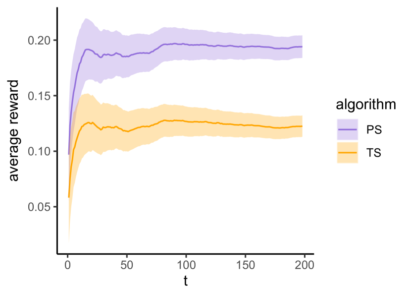
(f) $\gamma_{1}=0.3,\gamma_{2}=0.9$

Figure 8: Average reward collected by PS and that collected by TS in AR(1) bandits

References

• Agarwal, (2013) Agarwal, D. (2013). Computational advertising: the LinkedIn way. In Proceedings of the 22nd ACM international conference on Information & Knowledge Management, pages 1585–1586.
• Agarwal et al., (2014) Agarwal, D., Long, B., Traupman, J., Xin, D., and Zhang, L. (2014). Laser: A scalable response prediction platform for online advertising. In Proceedings of the 7th ACM international conference on Web search and data mining, pages 173–182.
• Agrawal and Goyal, (2012) Agrawal, S. and Goyal, N. (2012). Analysis of Thompson sampling for the multi-armed bandit problem. In Mannor, S., Srebro, N., and Williamson, R. C., editors, Proceedings of the 25th Annual Conference on Learning Theory, volume 23 of Proceedings of Machine Learning Research, pages 39.1–39.26, Edinburgh, Scotland. PMLR.
• (4) Arumugam, D. and Van Roy, B. (2021a). Deciding what to learn: A rate-distortion approach. In International Conference on Machine Learning, pages 373–382. PMLR.
• (5) Arumugam, D. and Van Roy, B. (2021b). The value of information when deciding what to learn. Advances in Neural Information Processing Systems, 34:9816–9827.
• Auer et al., (2002) Auer, P., Cesa-Bianchi, N., Freund, Y., and Schapire, R. E. (2002). The nonstochastic multiarmed bandit problem. SIAM journal on computing, 32(1):48–77.
• Bai et al., (2013) Bai, A., Wu, F., and Chen, X. (2013). Bayesian mixture modelling and inference based Thompson sampling in monte-carlo tree search. Advances in neural information processing systems, 26.
• Besbes et al., (2019) Besbes, O., Gur, Y., and Zeevi, A. (2019). Optimal exploration-exploitation in a multi-armed-bandit problem with non-stationary rewards. Stochastic Systems, 9(4):319–337.
• Besson and Kaufmann, (2019) Besson, L. and Kaufmann, E. (2019). The generalized likelihood ratio test meets KLUCB: an improved algorithm for piece-wise non-stationary bandits. Proceedings of Machine Learning Research vol XX, 1:35.
• Brown et al., (2010) Brown, D. B., Smith, J. E., and Sun, P. (2010). Information relaxations and duality in stochastic dynamic programs. Operations research, 58(4-part-1):785–801.
• Bubeck et al., (2015) Bubeck, S., Dekel, O., Koren, T., and Peres, Y. (2015). Bandit convex optimization:$\sqrt{T}$ regret in one dimension. In Conference on Learning Theory, pages 266–278. PMLR.
• Chapelle and Li, (2011) Chapelle, O. and Li, L. (2011). An empirical evaluation of Thompson sampling. In Shawe-Taylor, J., Zemel, R., Bartlett, P., Pereira, F., and Weinberger, K., editors, Advances in Neural Information Processing Systems, volume 24. Curran Associates, Inc.
• Cheung et al., (2019) Cheung, W. C., Simchi-Levi, D., and Zhu, R. (2019). Learning to optimize under non-stationarity. In The 22nd International Conference on Artificial Intelligence and Statistics, pages 1079–1087. PMLR.
• Dong and Van Roy, (2018) Dong, S. and Van Roy, B. (2018). An information-theoretic analysis for thompson sampling with many actions. Advances in Neural Information Processing Systems, 31.
• Ferreira et al., (2018) Ferreira, K. J., Simchi-Levi, D., and Wang, H. (2018). Online network revenue management using Thompson sampling. Operations research, 66(6):1586–1602.
• Freund and Banerjee, (2019) Freund, D. and Banerjee, S. (2019). Good prophets know when the end is near. Available at SSRN 3479189.
• Freund and Schapire, (1997) Freund, Y. and Schapire, R. E. (1997). A decision-theoretic generalization of on-line learning and an application to boosting. Journal of computer and system sciences, 55(1):119–139.
• Garivier and Moulines, (2008) Garivier, A. and Moulines, E. (2008). On upper-confidence bound policies for non-stationary bandit problems. arXiv preprint arXiv:0805.3415.
• Ghatak, (2021) Ghatak, G. (2021). A change-detection-based Thompson sampling framework for non-stationary bandits. IEEE Transactions on Computers, 70(10):1670–1676.
• Graepel et al., (2010) Graepel, T., Candela, J. Q., Borchert, T., and Herbrich, R. (2010). Web-scale Bayesian click-through rate prediction for sponsored search advertising in microsoft’s bing search engine. Omnipress.
• Gray, (2011) Gray, R. M. (2011). Entropy and information theory. Springer Science & Business Media.
• Gupta et al., (2011) Gupta, N., Granmo, O.-C., and Agrawala, A. (2011). Thompson sampling for dynamic multi-armed bandits. In 2011 10th International Conference on Machine Learning and Applications and Workshops, volume 1, pages 484–489. IEEE.
• Hao et al., (2022) Hao, B., Lattimore, T., and Qin, C. (2022). Contextual information-directed sampling. arXiv preprint arXiv:2205.10895.
• Hartland et al., (2006) Hartland, C., Gelly, S., Baskiotis, N., Teytaud, O., and Sebag, M. (2006). Multi-armed bandit, dynamic environments and meta-bandits.
• Hill et al., (2017) Hill, D. N., Nassif, H., Liu, Y., Iyer, A., and Vishwanathan, S. (2017). An efficient bandit algorithm for realtime multivariate optimization. In Proceedings of the 23rd ACM SIGKDD International Conference on Knowledge Discovery and Data Mining, pages 1813–1821.
• Kawale et al., (2015) Kawale, J., Bui, H. H., Kveton, B., Tran-Thanh, L., and Chawla, S. (2015). Efficient Thompson sampling for online matrix-factorization recommendation. Advances in neural information processing systems, 28.
• Kocsis and Szepesvári, (2006) Kocsis, L. and Szepesvári, C. (2006). Discounted UCB. In 2nd PASCAL Challenges Workshop, volume 2, pages 51–134.
• Kuhn et al., (2015) Kuhn, J., Mandjes, M., and Nazarathy, Y. (2015). Exploration vs exploitation with partially observable gaussian autoregressive arms. EAI Endorsed Transactions on Self-Adaptive Systems, 1(4).
• Kuhn and Nazarathy, (2015) Kuhn, J. and Nazarathy, Y. (2015). Wireless channel selection with reward-observing restless multi-armed bandits. Chapter to appear in “Markov Decision Processes in Practice”, Editors: R. Boucherie and N. van Dijk.
• Lai and Robbins, (1985) Lai, T. and Robbins, H. (1985). Asymptotically efficient adaptive allocation rules. Advances in Applied Mathematics, 6(1):4–22.
• Laplace, (1986) Laplace, P. S. (1986). Memoir on the probability of the causes of events. Statistical science, 1(3):364–378.
• Lattimore and Szepesvári, (2019) Lattimore, T. and Szepesvári, C. (2019). An information-theoretic approach to minimax regret in partial monitoring. In Conference on Learning Theory, pages 2111–2139. PMLR.
• Liu et al., (2022) Liu, Y., Devraj, A. M., Van Roy, B., and Xu, K. (2022). Gaussian imagination in bandit learning. arXiv preprint arXiv:2201.01902.
• Lu et al., (2021) Lu, X., Van Roy, B., Dwaracherla, V., Ibrahimi, M., Osband, I., and Wen, Z. (2021). Reinforcement learning, bit by bit. arXiv preprint arXiv:2103.04047.
• Mellor and Shapiro, (2013) Mellor, J. and Shapiro, J. (2013). Thompson sampling in switching environments with Bayesian online change detection. In Carvalho, C. M. and Ravikumar, P., editors, Proceedings of the Sixteenth International Conference on Artificial Intelligence and Statistics, volume 31 of Proceedings of Machine Learning Research, pages 442–450, Scottsdale, Arizona, USA. PMLR.
• Mesbah, (2018) Mesbah, A. (2018). Stochastic model predictive control with active uncertainty learning: A survey on dual control. Annual Reviews in Control, 45:107–117.
• Min et al., (2019) Min, S., Maglaras, C., and Moallemi, C. C. (2019). Thompson sampling with information relaxation penalties. Advances in Neural Information Processing Systems, 32.
• Neu et al., (2022) Neu, G., Olkhovskaya, J., Papini, M., and Schwartz, L. (2022). Lifting the information ratio: An information-theoretic analysis of thompson sampling for contextual bandits. arXiv preprint arXiv:2205.13924.
• Raj and Kalyani, (2017) Raj, V. and Kalyani, S. (2017). Taming non-stationary bandits: A Bayesian approach. arXiv preprint arXiv:1707.09727.
• Russo and Van Roy, (2014) Russo, D. and Van Roy, B. (2014). Learning to optimize via posterior sampling. Mathematics of Operations Research, 39(4).
• Russo and Van Roy, (2016) Russo, D. and Van Roy, B. (2016). An information-theoretic analysis of Thompson sampling. Journal of Machine Learning Research, 17(68):1–30.
• Russo and Van Roy, (2018) Russo, D. and Van Roy, B. (2018). Learning to optimize via information-directed sampling. Operations Research, 66(1):230–252.
• Russo and Van Roy, (2022) Russo, D. and Van Roy, B. (2022). Satisficing in time-sensitive bandit learning. Mathematics of Operations Research.
• Schwartz et al., (2017) Schwartz, E. M., Bradlow, E. T., and Fader, P. S. (2017). Customer acquisition via display advertising using multi-armed bandit experiments. Marketing Science, 36(4):500–522.
• Slivkins and Upfal, (2008) Slivkins, A. and Upfal, E. (2008). Adapting to a changing environment: the Brownian restless bandits. In COLT, pages 343–354.
• Spencer et al., (2014) Spencer, J., Sudan, M., and Xu, K. (2014). Queuing with future information. Annals of Applied Probability, 24(5):2091–2142.
• Thompson, (1933) Thompson, W. R. (1933). On the likelihood that one unknown probability exceeds another in view of the evidence of two samples. Biometrika, 25(3/4):285–294.
• Trovo et al., (2020) Trovo, F., Paladino, S., Restelli, M., and Gatti, N. (2020). Sliding-window Thompson sampling for non-stationary settings. Journal of Artificial Intelligence Research, 68:311–364.
• Turner et al., (2009) Turner, R., Saatci, Y., and Rasmussen, C. E. (2009). Adaptive sequential Bayesian change point detection. In Temporal Segmentation Workshop at NIPS, pages 1–4. Citeseer.
• Viappiani, (2013) Viappiani, P. (2013). Thompson sampling for Bayesian bandits with resets. In International Conference on Algorithmic Decision Theory, pages 399–410. Springer.
• Wen et al., (2022) Wen, Z., Osband, I. O., Qin, C., Lu, X., Ibrahimi, M., Dwaracherla, V., Asghari, M., and Van Roy, B. (2022). From predictions to decisions: The importance of joint predictive distributions. arXiv preprint arXiv:2107.09224.
• Wilson et al., (2010) Wilson, R. C., Nassar, M. R., and Gold, J. I. (2010). Bayesian online learning of the hazard rate in change-point problems. Neural computation, 22(9):2452–2476.
• Xu and Chan, (2016) Xu, K. and Chan, C. W. (2016). Using future information to reduce waiting times in the emergency department via diversion. Manufacturing & Service Operations Management, 18(3):314–331.