Numerical approximation of probabilistically weak and strong solutions of the stochastic total variation flow

Abstract.

We propose a fully practical numerical scheme for the simulation of the stochastic total variation flow (STFV). The approximation is based on a stable time-implicit finite element space-time approximation of a regularized STVF equation. The approximation also involves a finite dimensional discretization of the noise that makes the scheme fully implementable on physical hardware. We show that the proposed numerical scheme converges to a solution that is defined in the sense of stochastic variational inequalities (SVIs). As a by product of our convergence analysis we provide a generalization of the concept of probabilistically weak solutions of stochastic partial differential equation (SPDEs) to the setting of SVIs. We also prove convergence of the numerical scheme to a probabilistically strong solution in probability if pathwise uniqueness holds. We perform numerical simulations to illustrate the behavior of the proposed numerical scheme as well as its non-conforming variant in the context of image denoising.

1. Introduction

We study a numerical approximation of the stochastic total variation flow (STVF)

$$\mathrm{d}X =\mathrm{div}\left(\frac{\nabla X}{|\nabla X|}\right)\mathrm{d}t-\lambda(X-g)\mathrm{d}t+B(X)\mathrm{d}W, \text{in }(0,T)\times\mathcal{O},$$

(1) $$X =0 \text{on }(0,T)\times\partial\mathcal{O},$$

$$X(0) =x^{0} \text{in }\mathcal{O},$$

where $\mathcal{O}\subset\mathbb{R}^{d}$, $d\geq 1$ is a bounded polyhedral domain, $\lambda\geq 0$, $T>0$ are fixed constants and $x^{0},\,g\in\mathbb{L}^{2}$ are given functions. We consider $W$ to be a cylindrical Wiener process on $\ell_{2}$ and a continuous mapping $B:\mathbb{L}^{2}\to\mathscr{L}_{2}(\ell_{2};\mathbb{L}^{2})$ where $\mathscr{L}_{2}$ stands for the space of Hilbert-Schmidt operators such that

1. $\|B(h)\|_{\mathscr{L}_{2}(\ell_{2};\mathbb{L}^{2})}\leq C(\|h\|+1)$ for every $h\in\mathbb{L}^{2}$,

2. if $d\geq 2$, whenever $\{h_{n}\}$ is bounded in $\mathbb{L}^{2}$ and $h_{n}\to h$ a.e. in $\mathcal{O}$ then

   $$\|B(h_{n})-B(h)\|_{\mathscr{L}_{2}(\ell_{2};\mathbb{L}^{2})}\to 0.$$

We also consider the weakly lower semicontinuous energy functional $\mathcal{J}:\mathbb{L}^{2}\to[0,\infty]$

$$\mathcal{J}(u) :=\|\nabla u\|_{\operatorname{TV}(\mathcal{O})}+\int_{\partial\mathcal{O}}{|u|}\,\mathrm{d}x+\frac{\lambda}{2}\int_{\mathcal{O}}|u-g|^{2}\,\mathrm{d}x u \in\mathbb{L}^{2}\cap BV(O)\,,$$

$$\mathcal{J}(u) :=\infty u \in\mathbb{L}^{2}\setminus BV(O)\,,$$

see Lemma 8 for details.

Due to the singular character of total variation flow (1), it is convenient to perform numerical simulations using a regularized problem

$$\mathrm{d}X =\mathrm{div}\left(\frac{\nabla X}{\sqrt{|\nabla X|^{2}+\varepsilon^{2}}}\right)\mathrm{d}t-\lambda(X-g)\mathrm{d}t+{B(X)}\,\mathrm{d}W \text{in }(0,T)\times\mathcal{O},$$

(2) $$X =0 \text{on }(0,T)\times\partial\mathcal{O},$$

$$X(0) =x^{0} \text{in }\mathcal{O}\,,$$

with a regularization parameter $\varepsilon>0$. In the deterministic setting ($W\equiv 0$) the equation (1) corresponds to the gradient flow of the regularized energy functional

$$\mathcal{J}_{\varepsilon}(u):=\int_{\mathcal{O}}\sqrt{|\nabla u|^{2}+\varepsilon^{2}}\,\mathrm{d}x+\frac{\lambda}{2}\int_{\mathcal{O}}|u-g|^{2}\,\mathrm{d}x\qquad{u\in{\mathbb{H}^{1}_{0}}}.$$

Convergent finite element approximation of the deterministic total variation flow (i.e., (1) and (1) with $B(X)\equiv 0$) has been proposed in [12]. In the stochastic setting, numerical approximation of probabilistically strong SVI solutions of (1) with $B(X)\equiv X$ has been analyzed recently in [4, 6, 5] by considering the regularized problem (1) withing the framework of stochastic variational inequalities, cf. [2]. In the present work we propose a fully implementable numerical approximation of (1) via the regularized problem (1): in addition to the discretization in space and time we also consider an implementable approximation of the noise term. We show that, in the limit, the numerical solutions satisfy a stochastic variational inequality. As a consequence, we obtain an extension of the concept of stochastic variational inequalities of [2].

Let us compare the present work with [4] where (probabilistically) strong solutions of (1) are constructed numerically in case the domain $\mathcal{O}$ is bounded, convex and with a piecewise $C^{2}$-smooth boundary, the equation is driven by a one-dimensional noise $W$, $B(X)=X$ and the interpolants $\overline{X}^{\varepsilon}_{\tau,h}$ of the numerical approximations converge to the unique solution $X$ with paths continuous in $L^{2}(\mathcal{O})$ via the double limit

$$\lim_{\varepsilon\to 0}\lim_{(\tau,h)\to(0,0)}\|\overline{X}^{\varepsilon}_{\tau,h}-X\|_{L^{2}(\Omega\times(0,T);L^{2}(\mathcal{O}))}=0.$$

In the present work $\mathcal{O}$ is an open convex polyhedral domain, $B$ is a fairly general non-linearity (hence uniqueness is not expected to hold and we construct just (probabilistically weak) “martingale” solutions). Furthermore, the considered noise is an infinite dimensional random walk generated by a sequence of random variables (suitable for computer simulations) and $\overline{X}^{\varepsilon}_{\tau,h}$ converge to $X$ in the joint limit as $(\varepsilon,\tau,h)\to(0,0,0)$. Our SVI solution concept is more general than the one in [4] but paths of the obtained solutions are only weakly continuous in $L^{2}(\mathcal{O})$ and we cover the case $B(X)=X$ only in $d=1$. If, in addition, pathwise uniqueness holds then the approximations converge to a probabilistically strong solution in probability. We also note that the technique used for the construction of the probabilistically weak SVI solutions is straightforward, i.e., we avoid the use of martingale and Skorokhod representation theorems as in [17].

The paper is organized as follows. In Section 2 we introduce the notation and the numerical approximation of (1) and in Section 3 we state the main results of the paper (which are proven in Sections 7 and 8). In Section 4 we show a priori estimate for the numerical solution. In Section 5 we present auxiliary results on compactness properties of locally convex spaces which are used to deduce tightness properties and convergence of the numerical approximation in Section 6. Numerical experiments for the conforming and non-conforming finite element approximation schemes are presented in Section 9. The proofs of auxiliary results are collected in the Appendix.

2. Numerical approximation

We denote the stanandard Lebesque and Sobolev functions spaces on $\mathcal{O}$ as $\mathbb{L}^{2}:={L}^{2}(\mathcal{O})$, $\mathbb{L}^{2}_{w}=(\mathbb{L}^{2},weak)$, $\mathbb{H}^{1}_{0}:={H}^{1}_{0}(\mathcal{O})$, $\mathbb{W}^{1,1}:={W}^{1,1}(\mathcal{O})$. The sets of rational and irrational numbers are denoted as $\mathbb{Q}$ and $\mathbb{Q}^{\complement}$, respectively. For time dependent random variables we often write $S_{t}(\cdot)$ instead of $S(\cdot,t)$ provided that it fits the context of presentation.

For $u\in BV(\mathcal{O})$, the gradient $\nabla u$ is a vector measure whose total variation satisfies

(3) $$\|\nabla u\|_{\operatorname{TV}(\mathcal{O})}=\sup\left\{-\int_{\mathcal{O}}u\,\mathrm{div}\,\mathbf{v}\mathrm{d}x;~{}\mathbf{v}\in C^{\infty}_{0}(\mathcal{O},\mathbb{R}^{d}),~{}\|\mathbf{v}\|_{\mathbb{L}^{\infty}}\leq 1\right\}$$

and we define, as usual,

$$\|u\|_{BV(\mathcal{O})}:=\|u\|_{\mathbb{L}^{1}}+\|\nabla u\|_{\operatorname{TV}(\mathcal{O})},\qquad u\in BV(\mathcal{O}).$$

For $N\in\mathbb{N}$ we consider a discrete filtration $\mathcal{F}_{\tau}:=\{\mathcal{F}^{i}_{\tau}\}_{i=0}^{N}$ on a probability space $(\Omega_{\tau},\mathscr{F}_{\tau},\mathbb{P}_{\tau})$ and sequence $\{\xi^{i,j}_{\tau}\}_{i,j=1}^{N}$ of independent random variables such that

• $\mathbb{E}\left[\,\xi^{i,j}_{\tau}\right]=0$,

• $\mathbb{E}\left[\,|\xi^{i,j}_{\tau}|^{2}\right]=\tau$,

• $\mathbb{E}\left[\,|\xi^{i,j}_{\tau}|^{4}\right]\leq C\tau^{2}$,

• $(\xi^{i,1}_{\tau},\dots,\xi^{i,N}_{\tau})$ is $\mathcal{F}^{i}_{\tau}$-measurable and independent of $\mathcal{F}^{i-1}_{\tau}$,

for every $i,j\in\{1,\dots,N\}$ and some fixed constant $C>0$ independent of $N\in\mathbb{N}$. A simple and easily implementable construction of the noise that satisfies the above properties is, for instance, $\xi^{i,j}_{\tau}=\sqrt{\tau}\chi^{i,j}$ where $\{\chi^{i,j}\}_{i,j=1}^{N}$ are independent with $\mathbb{P}\,[\chi^{i,j}=\pm 1]=\frac{1}{2}$; as another choice, one can consider Brownian increments $\xi^{i,j}_{\tau}=\Delta_{i}\beta^{j}:=\beta^{j}(t_{i})-\beta^{j}(t_{i-1})$ of independent Brownian motions $\beta^{j}$.

Let $\mathbb{V}_{h}\subset\mathbb{H}^{1}_{0}$ be the standard finite element space of globally continuous functions which are piecewise linear over a quasi-uniform partition $\mathcal{T}_{h}$ of $\mathcal{O}$ and let $P_{h}:\mathbb{L}^{2}\rightarrow\mathbb{V}_{h}$ denote the $\mathbb{L}^{2}$-orthogonal projection on $\mathbb{V}_{h}$. We assume that the finite element space satisfies the following properties.

Assumption 1.

1. $\mathbb{V}_{h}$ is a finite-dimensional subspace of $\mathbb{H}^{1}_{0}$,

2. $\mathbb{V}_{h_{2}}\subseteq\mathbb{V}_{h_{1}}$ if $0<h_{1}<h_{2}$,

3. $\|P_{h}v\|_{\mathbb{H}^{1}_{0}}\leq\kappa\|v\|_{\mathbb{H}^{1}_{0}}$ holds for every $v\in\mathbb{H}^{1}_{0}$ and $h>0$, for some $\kappa\in(0,\infty)$ (see [9]),

4. $\bigcup_{h>0}\mathbb{V}_{h}$ is dense both in $\mathbb{H}^{1}_{0}$ and $\mathbb{L}^{2}$.

It is well-know that the above assumption is satisfied for $\mathbb{V}_{h}$, $P_{h}$ see for instance [11]. We note that the stability of the $\mathbb{L}^{2}$-projection, Assumption 1₍₃₎ and the density of $\{\mathbb{V}_{h}\}_{h>0}$ in $\mathbb{H}^{1}_{0}$ implies that $\|\nabla v-\nabla P_{h}v\|\rightarrow 0$ as $h\rightarrow 0$ for every $v\in\mathbb{H}^{1}_{0}$.

We consider the following fully-discrete approximation of (1): fix $N\in\mathbb{N}$, $h>0$ set $X^{0}=P_{h}x^{0}$ and determine $X^{i}\in\mathbb{V}_{h}$, $i=1,\dots,N$ as the solution of

(4) $$\left(X^{i}-X^{i-1},v_{h}\right)= -\tau\left(\frac{\nabla X^{i}}{\sqrt{|\nabla X^{i}|^{2}+\varepsilon^{2}}},\nabla v_{h}\right)$$

$$-\tau\lambda\left(X^{i}-{g},v_{h}\right)+{\sum_{j=1}^{N}\left(B_{j}(X^{i-1}),v_{h}\right)\xi^{i,j}_{\tau}} \forall v_{h}\in\mathbb{V}_{h}.$$

Existence of the unique $\mathcal{F}_{\tau}$-adapted $\mathbb{V}_{h}$-valued solution $\{X^{i}\}_{i=0}^{N}$ can be proved analogically to [4, Lemma 3] therefore we omit the proof. The process $X^{i}\equiv X^{i}_{\varepsilon,h}$, $i=0,\dots,N$ depends on the parameters $(\tau,h,\varepsilon)$, to simplify the notation we suppress this dependence unless it matters.

3. Summary of the main results

In this section, we summarize the main results of the paper. We start with the definition of the SVI solution of (1).

Definition 1.

Let $(\Omega,\mathcal{F},(\mathcal{F}_{t}),\mathbb{P})$ be a stochastic basis with independent $(\mathcal{F}_{t})$-Wiener processes $(W^{k})_{k\in\mathbb{N}}$. An adapted process $X{\in L^{2}([0,T]\times\Omega;\mathbb{L}^{2})}$ with weakly continuous paths in $\mathbb{L}^{2}$ is called an SVI solution of (1) provided that

(5) $$\frac{1}{2}\mathbb{E}\left[\|X(t)-I(t)\|^{2}\right] +\mathbb{E}\left[\int_{0}^{t}\mathcal{J}(X(s))\,\mathrm{d}s\right]\leq\frac{1}{2}\|x^{0}-u^{0}\|^{2}$$

$$+\mathbb{E}\left[\int_{0}^{t}\mathcal{J}(I(s))\,\mathrm{d}s\right]+\mathbb{E}\left[\int_{0}^{t}(G(s),X(s)-I(s))\,\mathrm{d}s\right]$$

$$+\frac{1}{2}\mathbb{E}\left[\int_{0}^{t}\|B(X(s))-H(s)\|_{\mathscr{L}_{2}(\ell_{2},\mathbb{L}^{2})}^{2}\,\mathrm{d}s\right]\,,$$

holds for every $t\in[0,T]$ and for every test process

(6) $$I(t)=u^{0}{-}\int_{0}^{t}G(s)\,\mathrm{d}s+\sum_{j=1}^{\infty}\int_{0}^{t}H_{j}(s)\,\mathrm{d}W^{j},\qquad t\in[0,T]\,,$$

that satisfies $\mathbb{P}\,[I(t)\in\mathbb{H}^{1}_{0}]=1$ for almost every $t\in[0,T]$ and

$$\mathbb{E}\left[\int_{0}^{T}\|I(t)\|_{\mathbb{H}^{1}_{0}}\,\mathrm{d}t\right]<\infty\,,$$

for some $u^{0}\in\mathbb{L}^{2}$ and $(\mathcal{F}_{t})$-progressively measurable processes $G$ and $H$ in $L^{2}([0,T]\times\Omega;\mathbb{L}^{2})$ and $L^{2}([0,T]\times\Omega;\mathscr{L}_{2}(\ell_{2},\mathbb{L}^{2}))$ respectively.

Remark 1.

Inequality (5) implies

$$\sup_{t\in{0,T}}\mathbb{E}\left[\|X(t)\|^{2}\right]+\mathbb{E}\left[\int_{0}^{T}\|X(t)\|_{BV(\mathcal{O})}\right]\,\mathrm{d}t<\infty.$$

Remark 2.

The SVI solution in the sense of Definition 1 generalizes the definition of the SVI solution from [2] since the inequality (5) holds for a much larger class of test processes introduced in (6) than in [2].

We define the piecewise linear interpolant of the solution of the scheme (4) as

(7) $$X_{\tau}(t)=\frac{t-t_{i-1}}{\tau}X^{i}+\frac{t_{i}-t}{\tau}X^{i-1}\quad\mathrm{for}\,\,t\in[t_{i-1},t_{i}]\,,$$

as well as the piecewise constant interpolants

(8a) $$\overline{X}_{\tau}(t) =X^{i}\quad\mathrm{for}\,\,t\in(t_{i-1},t_{i})\,,$$

(8b) $$\underline{X}_{\tau}(t) =X^{i-1}\quad\mathrm{for}\,\,t\in(t_{i-1},t_{i})\,,$$

where the dependence on $\varepsilon$, $h$ is not displayed.

Let $\mathcal{X}^{(1)}$ denote the space of weakly càglàd functions $f:[0,T]\to\mathbb{L}^{2}$ such that

$$\int_{0}^{T}\|f(s)\|_{BV(\mathcal{O})}\,ds<\infty,$$

let $\mathcal{X}^{(2)}$ denote the space of weakly càdlàg functions $f:[0,T]\to\mathbb{L}^{2}$, define $\mathcal{X}^{(3)}$ as $C([0,T];\mathbb{L}^{2}_{w})$ and equip the spaces $\mathcal{X}^{(1)}$, $\mathcal{X}^{(2)}$ and $\mathcal{X}^{(3)}$ with the topology of uniform convergence in $\mathbb{L}^{2}_{w}$.

Theorem 1.

The random variables

$$(\overline{X}_{\varepsilon,h,\tau},\underline{X}_{\varepsilon,h,\tau},X_{\varepsilon,h,\tau}):(\Omega_{\tau},\mathcal{F}_{\tau},\mathbb{P}_{\tau})\to\mathcal{X}^{(1)}\times\mathcal{X}^{(2)}\times\mathcal{X}^{(3)}\,,$$

are Borel measurable, their laws under $\mathbb{P}_{\tau}\equiv\mathbb{P}_{\varepsilon,h,\tau}$ are tight with respect to $\varepsilon$, $h$, $\tau$ and, moreover, every sequence $(\varepsilon_{n},h_{n},\tau_{n})\to(0,0,0)$ has a subsequence $(\varepsilon_{n_{k}},h_{n_{k}},\tau_{n_{k}})$ such that laws of

$$(\overline{X}_{\varepsilon_{n_{k}},h_{n_{k}},\tau_{n_{k}}},\underline{X}_{\varepsilon_{n_{k}},h_{n_{k}},\tau_{n_{k}}},X_{\varepsilon_{n_{k}},h_{n_{k}},\tau_{n_{k}}})$$

under $\mathbb{P}_{\tau_{n_{k}}}$ converge to a Radon probability measure $\nu$ on $\mathscr{B}(\mathcal{X}^{(1)}\times\mathcal{X}^{(2)}\times\mathcal{X}^{(3)})$ that satisfies

$$\nu\big{(}(x_{1},x_{2},x_{3})\in\mathcal{X}^{(1)}\times\mathcal{X}^{(2)}\times\mathcal{X}^{(3)}:\,x_{1}=x_{2}=x_{3}\big{)}=1\,,$$

and there exists a stochastic basis $(\Omega,\mathcal{F},(\mathcal{F}_{t}),\mathbb{P})$ with independent $(\mathcal{F}_{t})$-Wiener processes $(W^{k})_{k\in\mathbb{N}}$ and a weakly continuous $\mathbb{L}^{2}$-valued SVI solution $X$ of (1) in the sense of Definition 1 such that $X(0)=x^{0}$, $\nu$ is the law of $(X,X,X)$ on $\mathcal{X}^{(1)}\times\mathcal{X}^{(2)}\times\mathcal{X}^{(3)}$ and

(9) $$\mathbb{E}\left[\sup_{t\in[0,T]}\|X(t)\|^{4}+\left(\int_{0}^{T}\|X(s)\|_{BV(\mathcal{O})}\,\mathrm{d}s\right)^{2}\right]\leq C$$

where $C$ depends only on $\|x_{0}\|$, $|\mathcal{O}|$, and $\|g\|$.

Proof.

See Corollary 3 and Theorem 5 for the proof. ∎

Remark 3.

Compared to the (probabilistically strong) SVI solutions in [2], [4] where the stochastic basis is given, the SVI solution obtained in this paper is probabilistically weak in the sense that $(\Omega,\mathcal{F},(\mathcal{F}_{t}),\mathbb{P})\equiv(\mathbf{Z},\mathscr{B}(\mathbf{Z}),(\mathcal{Z}^{\mu}_{t}),\mu)$ is constructed as a part of the solution, cf. Corollary 3 and Theorem 5.

Remark 4.

If uniqueness in law holds for the SVI solution of (1), cf. [2], then the laws of

$$(\overline{X}_{\varepsilon,h,\tau},\underline{X}_{\varepsilon,h,\tau},X_{\varepsilon,h,\tau})$$

under $\mathbb{P}_{\tau}$ converge to $\nu$ on $\mathscr{B}(\mathcal{X}^{(1)}\times\mathcal{X}^{(2)}\times\mathcal{X}^{(3)})$ as $(\varepsilon,h,\tau)\to(0,0,0)$, in particular, there is no need to pass to a subsequence in Theorem 1.

In case we work on a single stochastic basis with a given Wiener process and pathwise uniqueness holds for (1) then we can construct probabilistically strong solutions.

Theorem 2.

Let $(W^{j})_{j\in\mathbb{N}}$ be independent $(\mathcal{F}_{t})$-Wiener processes on $(\Omega,\mathcal{F},(\mathcal{F}_{t}),\mathbb{P})$ and let

$$\xi_{\tau}^{i,j}=W^{j}(t_{i})-W^{j}(t_{i-1}),\qquad t_{i}=i\tau.$$

Furthremore, assume that pathwise uniqueness holds for the SVI solutions of (1) satisfying (9). Then there exists an SVI solution $X$ with respect to $(W^{j})_{j\in\mathbb{N}}$ satisfying (9) such that

$$\sup_{t\in[0,T]}|(\overline{X}_{\varepsilon,h,\tau}(t)-X(t),\varphi)|,\qquad\sup_{t\in[0,T]}|(\underline{X}_{\varepsilon,h,\tau}(t)-X(t),\varphi)|,\quad\sup_{t\in[0,T]}|(X_{\varepsilon,h,\tau}(t)-X(t),\varphi)|$$

converge to $0$ in probability as $(\varepsilon,h,\tau)\to(0,0,0)$ for every $\varphi\in\mathbb{L}^{2}$.

Proof.

See Theorem 6. ∎

Remark 5.

Theorem 1 and Theorem 2 can be strengthened considerably by Lemma 7. Assume that

$$K:\mathcal{X}^{(1)}\times\mathcal{X}^{(1)}\times\mathcal{X}^{(2)}\times\mathcal{X}^{(3)}\to[0,\infty]$$

satisfies the following property:

(10) $$K(f^{0},f^{1},g,h)\leq\liminf_{n\to\infty}K(f^{0}_{n},f^{1}_{n},g_{n},h_{n})$$

for any sequence $(f^{0}_{k},f^{1}_{k},g_{k},h_{k})\in\mathcal{X}^{(1)}\times\mathcal{X}^{(1)}\times\mathcal{X}^{(2)}\times\mathcal{X}^{(3)}$ converging in $\mathcal{X}^{(1)}\times\mathcal{X}^{(1)}\times\mathcal{X}^{(2)}\times\mathcal{X}^{(3)}$ to $(f^{0},f^{1},g,h)$ where in addition

$$\sup_{k}\int_{0}^{T}[\|f^{0}_{k}(s)\|_{BV(\mathcal{O})}+\|f^{1}_{k}(s)\|_{BV(\mathcal{O})}]\,\mathrm{d}s<\infty\,.$$

Then the variables $(\overline{X}_{\varepsilon_{n_{k}},h_{n_{k}},\tau_{n_{k}}},\underline{X}_{\varepsilon_{n_{k}},h_{n_{k}},\tau_{n_{k}}},X_{\varepsilon_{n_{k}},h_{n_{k}},\tau_{n_{k}}})$ from Theorem 1 satisfy

(11) $$\mathbb{E}\left[K(X,X,X,X)\right]\leq\liminf_{k\to\infty}\mathbb{E}_{\tau_{k}}\left[K(\overline{X}_{\varepsilon_{n_{k}},h_{n_{k}},\tau_{n_{k}}},\overline{X}_{\varepsilon_{n_{k}},h_{n_{k}},\tau_{n_{k}}},\underline{X}_{\varepsilon_{n_{k}},h_{n_{k}},\tau_{n_{k}}},X_{\varepsilon_{n_{k}},h_{n_{k}},\tau_{n_{k}}})\right]$$

and the random variables $(X,\overline{X}_{\varepsilon,h,\tau},\underline{X}_{\varepsilon,h,\tau},X_{\varepsilon,h,\tau})$ from Theorem 2 satisfy

(12) $$\mathbb{E}\left[K(X,X,X,X)\right]\leq\liminf_{(\varepsilon,h,\tau)\to(0,0,0)}\mathbb{E}\left[K(X,\overline{X}_{\varepsilon,h,\tau},\underline{X}_{\varepsilon,h,\tau},X_{\varepsilon,h,\tau})\right].$$

Obviously, if $K$ is real bounded and (10) holds also for $-K$ then we get equalities and limits in (11) and (12). In particular, under the assumptions of Theorem 2,

$$\|\overline{X}_{\varepsilon,h,\tau}-X\|_{L^{q}((0,T);L^{r}(\mathcal{O}))}\to 0$$

in probability as $(\varepsilon,h,\tau)\to(0,0,0)$ for every $r\in[1,\frac{d}{d-1})$ and every $q\in[1,\infty)$ such that $q(r-2)<r$.

4. A priori estimates

The numerical approximation (4) satisfies a discrete energy estimate.

Lemma 1.

Let $x^{0},g\in\mathbb{L}^{2}$ and $T>0$. Then there exists a constant $C>0$ depending only on $T$ and on the constants in $(\mathbf{B}_{1})$ and in Section 2 such that the solutions of scheme (4) satisfy for any $\varepsilon,h\in(0,1]$, $N\in\mathbb{N}$

(13) $$\mathbb{E}\,\Big{[}\frac{1}{2}\sup_{i=1,\ldots,N}\|X^{i}\|^{2}+\sum_{i=1}^{N}\Big{(}\frac{1}{4}\|X^{i}-X^{i-1}\|^{2} +\tau\mathcal{J}_{\varepsilon}(X^{i})\Big{)}\Big{]}^{2}$$

$$\leq{C}\left({\frac{1}{2}}+\frac{1}{2}\|x^{0}\|^{2}+|\mathcal{O}|+\frac{\lambda}{2}\|g\|^{2}\right)^{2}.$$

Proof.

Analogically to [4, Lemma 4.9], set $v_{h}=X^{i}$ in (4) and obtain

$$\frac{1}{2}\|X^{i}\|^{2}-\frac{1}{2}\|X^{i-1}\|^{2} +\frac{1}{4}\|X^{i}-X^{i-1}\|^{2}+\tau\mathcal{J}_{\varepsilon}(X^{i})$$

$$\leq \tau\mathcal{J}_{\varepsilon}(0)+\sum_{j=1}^{N}(B_{j}(X^{i-1}),X^{i-1})\xi^{i,j}_{\tau}+\left\|\sum_{j=1}^{N}B_{j}(X^{i-1})\xi^{i,j}_{\tau}\right\|^{2}$$

for $1\leq i\leq N$. If we define

$$a^{i} =\frac{1}{2}+\frac{1}{2}\|X^{i}\|^{2}+\sum_{j=1}^{i}\left(\frac{1}{4}\|X^{j}-X^{j-1}\|^{2}+\tau\mathcal{J}_{\varepsilon}(X^{j})\right)$$

$$b =\tau\mathcal{J}_{\varepsilon}(0),\quad c^{i}=\sum_{j=1}^{N}(B_{j}(X^{i-1}),X^{i-1})\xi^{i,j}_{\tau},\quad d^{i}=\left\|\sum_{j=1}^{N}B_{j}(X^{i-1})\xi^{i,j}_{\tau}\right\|^{2}\,,$$

then

$$a^{i}-a^{i-1}\leq b+c^{i}+d^{i},\qquad i=1,\dots,N.$$

If $a^{i-1}\in L^{2}(\Omega)$ then $X^{i-1}\in L^{4}(\Omega;\mathbb{L}^{2})$, $c^{i}\in L^{2}(\Omega)$, $d^{i}\in L^{2}(\Omega)$ and so, by induction, $a^{i}\in L^{2}(\Omega)$ for every $i=0,\dots,N$. Next, observe that $c^{i}$ is a square integrable martingale difference and that

$$\mathbb{E}\left[(c^{i})^{2}\right]\leq C_{B}\tau\mathbb{E}\left[(a^{i-1})^{2}\right],\qquad\mathbb{E}\left[(d^{i})^{2}\right]\leq C_{B}\tau^{2}\mathbb{E}\left[(a^{i-1})^{2}\right]$$

where $C_{B}$ depends only on the growth constants in $(\mathbf{B}_{1})$ and in the assumption $\mathbb{E}\left[(\xi^{i,j}_{\tau})^{2}\right]\leq C\tau^{2}$. Let us define

$$a_{*}^{i}=\max_{j=0,\dots,i}a^{j},\qquad i=0,\dots,N.$$

Then

$$a_{*}^{i}\leq(a^{0}+Nb)+{\max_{j=1,\dots,i}}\left|\sum_{\ell=1}^{j}c^{\ell}\right|+\sum_{j=1}^{i}d^{j},\qquad i=1,\dots,N$$

and

$$(a_{*}^{i})^{2}\leq 3(a^{0}+Nb)^{2}+3{\max_{j=1,\dots,i}}\left|\sum_{\ell=1}^{j}c^{\ell}\right|^{2}+3N\sum_{j=1}^{i}(d^{j})^{2},\qquad i=1,\dots,N.$$

Hence, by the discrete Burkholder-Davis-Gundy inequality, we obtain

$$\mathbb{E}\left[(a_{*}^{i})^{2}\right] \leq 3(a^{0}+Nb)^{2}+3C_{2}\sum_{j=1}^{i}\mathbb{E}\left[(c^{j})^{2}\right]+3N\sum_{j=1}^{i}\mathbb{E}\left[(d^{j})^{2}\right]$$

$$\leq 3(a^{0}+Nb)^{2}+3C_{2}\mathbf{c}\tau\sum_{j=1}^{i}\mathbb{E}\left[(a^{j-1})^{2}\right]+3\mathbf{c}\tau^{2}N\sum_{j=1}^{i}\mathbb{E}\left[(a^{j-1})^{2}\right]$$

$$\leq 3(a^{0}+Nb)^{2}+\frac{K_{C,T}}{N}\sum_{j=1}^{i}\mathbb{E}\left[(a_{*}^{j-1})^{2}\right],\qquad i=1,\dots,N$$

and we get the result by the discrete Gronwall lemma.

∎

Next, we estimate the discrete time increments of the numerical solution.

Lemma 2.

For any $0\leq n\leq\ell+n\leq N$ it holds that

$$\mathbb{E}[\|X^{n+\ell}-X^{n}\|_{\mathbb{H}^{-1}}^{4}]\leq Ct_{\ell}^{2}\,,$$

where $C$ does not depend on $\varepsilon$, $h$, $\tau$.

Proof.

For any $v\in\mathbb{H}^{1}_{0}$ we set $v_{h}=P_{h}v$ in (4) and get after summing up for $i=n+1,\dots,n+\ell$ by the definition of projection $P_{h}$ that

$$\left(X^{n+\ell}-X^{n},v_{h}\right)=\left(X^{n+\ell}-X^{n},P_{h}v\right)\leq\tau\sum_{i=n+1}^{n+\ell}\left\|\frac{\nabla X^{i}}{\sqrt{|\nabla X^{i}|^{2}+\varepsilon^{2}}}\right\|\|\nabla P_{h}v\|$$

$$\qquad+\tau\sum_{i=n+1}^{n+\ell}\lambda\big{(}\|X^{i}\|+\|{g}\|\big{)}\|P_{h}v\|+\Big{\|}\sum_{i=n+1}^{n+\ell}\sum_{j=1}^{N}B_{j}(X^{i-1})\xi^{i,j}_{\tau}\Big{\|}\|P_{h}v\| \forall v\in\mathbb{H}^{1}_{0}.$$

On noting that that $\left|\frac{\nabla\cdot}{\sqrt{|\nabla\cdot|^{2}+\varepsilon^{2}}}\right|\leq 1$ we deduce by the stability of the $\mathbb{L}^{2}$ projection $\|P_{h}v\|_{\mathbb{H}^{1}_{0}}\leq\kappa\|v\|_{\mathbb{H}^{1}_{0}}$ that

$$\|X^{n+\ell}-X^{n}\|_{\mathbb{H}^{-1}}\leq Ct_{\ell}[1+\max_{i=1,\dots,N}\,\{\|X^{i}\|\})]+\left\|\sum_{i=n+1}^{n+\ell}\sum_{j=1}^{N}B_{j}(X^{i-1})\xi^{i,j}_{\tau}\right\|\,.$$

Hence, we obtain

$$\mathbb{E}\left[\|X^{n+\ell}-X^{n}\|^{4}_{\mathbb{H}^{-1}}\right]\leq ct^{4}_{\ell}+ct^{2}_{\ell}\,,$$

by the Burkholder-Rosenthal inequality, Lemma 1 and linear growth of $B:\mathbb{L}^{2}\to\mathscr{L}_{2}(\ell_{2};\mathbb{L}^{2})$. Indeed, the martingale difference

$$d_{i}=\sum_{j=1}^{N}B_{j}(X^{i-1})\xi^{i,j}_{\tau}\,,$$

satisfies for $p\in\{2,4\}$

$$\sum_{i=n+1}^{n+l}\mathbb{E}\,\left[\|d_{i}\|^{p}|\mathcal{F}^{i-1}_{\tau}\right] \leq c_{\kappa}\tau^{\frac{p}{2}}\sum_{i=n+1}^{n+l}\left[\sum_{j=1}^{N}\|B_{j}(X^{i-1})\|^{2}\right]^{\frac{p}{2}}\leq c_{\kappa}\tau^{\frac{p}{2}}\sum_{i=n+1}^{n+l}\|B(X^{i-1})\|^{p}_{\mathscr{L}_{2}(\ell_{2};\mathbb{L}^{2})}$$

$$\leq c_{\kappa}\tau^{\frac{p}{2}}\sum_{i=n+1}^{n+l}[1+\|X^{i-1}\|]^{p}\leq c_{\kappa}t^{\frac{p}{2}}_{\ell}[1+\max_{i=1,\dots,N}\,\{\|X^{i}\|^{p}\}].$$

∎

Lemma 3.

Let $u^{0}\in\mathbb{V}_{h}$, let $G^{1},\dots,G^{N}$ and $H^{0,j},\dots,H^{N-1,j}$ be $\mathcal{F}_{\tau}$-adapted random variables in $L^{2}(\Omega;\mathbb{V}_{h})$ for every $j\in\{1,\dots,N\}$ and define

(14) $$U^{i}=u^{0}-\tau\sum_{\ell=1}^{i}G^{\ell}+\sum_{\ell=1}^{i}\sum_{j=1}^{N}H^{\ell-1,j}\xi^{\ell,j}_{\tau},\qquad i\in\{0,\dots,N\}.$$

Then

$$\frac{1}{2}\mathbb{E}\left[\|X^{i}-U^{i}\|^{2}\right]+\tau\sum_{\ell=1}^{i}\mathbb{E}\left[\mathcal{J}_{\varepsilon}(X^{\ell})\right] \leq\frac{1}{2}\|x^{0}-u^{0}\|^{2}+\tau\sum_{\ell=1}^{i}\mathbb{E}\left[\mathcal{J}_{\varepsilon}(U^{\ell})+(G^{\ell},X^{\ell}-U^{\ell})\right]$$

$$+\frac{\tau}{2}\sum_{\ell=1}^{i}\sum_{j=1}^{N}\mathbb{E}\left[\|P_{h}B_{j}(X^{\ell-1})-H^{\ell-1,j}\|^{2}\right],\quad 0\leq i\leq N.$$

Proof.

We denote $D^{i}=X^{i}-U^{i}$ and use (4), (14) to deduce the formula for $(D^{i}-D^{i-1},v_{h})$ for $v_{h}\in\mathbb{V}_{h}$. We then set $v_{h}=D^{i}$, use that $(B_{j}(X^{i-1}),D^{i})=(P_{h}B_{j}(X^{i-1}),D^{i})$ and proceed as in the proof of Lemma 1. ∎

5. Compactness in locally convex path spaces

In this section, $Y$ stands for a Hausdorff locally convex space (typically a Hilbert space equipped with the strong or the weak topology), $Y^{[0,T]}$ denotes the space of functions from $[0,T]$ to $Y$ on which we consider the topology of uniform convergence $\tau_{\mathbf{u}}$. We also define the subspaces $Q_{n}([0,T];Y)$, $n\in\mathbb{N}$ spanned by the functions $f\in Y^{[0,T]}$ that are constant on every interval $(t_{i-1}^{n},t^{n}_{i})$ for $1\leq i\leq n$ where $t^{k}_{j}=jT/k$, the Hausdorff locally convex path spaces

$$Q_{\infty}([0,T];Y)=\bigcup_{n=1}^{\infty}Q_{n}([0,T];Y),\qquad Q([0,T];Y)=\overline{Q_{\infty}([0,T];Y)}\,,$$

and an important $F_{\sigma}$ subset of $Q([0,T];Y)$

$$Q_{c}([0,T];Y)=Q_{\infty}([0,T];Y)\cup C([0,T];Y)\,,$$

that contains both step-functions on equidistant partitions of $[0,T]$ and continuous functions, equipped with the uniform convergence topology, that is best suitable for our purposes in the sequel when piecewise constant processes will converge uniformly to a continuous process. The space of continuous $Y$-valued functions $C([0,T];Y)$ is also equipped with the topology of uniform convergence.

Further, we define the space

$$Q_{c,BV}([0,T];\mathbb{L}^{2}_{w})=\left\{f\in Q_{c}([0,T];\mathbb{L}^{2}_{w}):\,\int_{0}^{T}\|f(s)\|_{BV(\mathcal{O})}\,ds<\infty\right\}\,,$$

as an $F_{\sigma}$ subset of $Q([0,T];\mathbb{L}^{2}_{w})$.

Finally, if $M$ is a subset of $Q([0,T];Y)$, we define

$$M^{\uparrow}_{n}=M\setminus\bigcup_{m=1}^{n-1}Q_{m}([0,T];Y).$$

Remark 6.

Every $f\in Q([0,T];Y)$, as a uniform limit of functions in $Q_{\infty}([0,T];Y)$, is bounded and also continuous at every $x=Tr$ for some irrational number $r$. In particular, $f$ is continuous with an exception of an at most countable set and, as such, $f$ is Borel measurable.

Remark 7.

If $Y$ is sequentially complete then $Q([0,T];Y)$ coincides with the space of functions $f\in Y^{[0,T]}$ that are continuous at every $t\in(T\mathbb{Q}^{\complement})\cap[0,T]$ and that have right and left limits at every $t\in[0,T]$.

Remark 8.

The space $Q([0,T];Y)$ can be also equipped (alternatively) with the Skorokhod topology defined by neighbourhoods

$$N_{O,\varepsilon}(f)=\{g:\,\exists\mu\text{ such that }\gamma(\mu)<\varepsilon\text{ and }g(\mu(t))-f(t)\in O\text{ for every }t\in[0,T]\}$$

where $O$ is an absolutely convex neighbourhood of zero in $Y$, $\varepsilon>0$, $\mu$ is an increasing bi-Lipschitz continuous homeomorphisms of $[0,T]$ onto $[0,T]$ and $\gamma(\mu)=\|\log\mu^{\prime}\|_{L^{\infty}}$. But the Skorokhod topology is strictly weaker than the topology of uniform convergence. In other words, convergence in $Q([0,T];Y)$ implies convergence in the Skorokhod topology but not vice versa. Thus, for our purposes, the space $Q([0,T];Y)$ with the topology of uniorm convergence is the better choice.

In the next theorem, we characterize compact sets in $Q_{c}([0,T];Y)$ which play an essential role in this paper. To this end, we present an Arzela-Ascoli theorem.

Theorem 3.

Let $M$ be a non-empty subset in $Q([0,T];Y)$ and consider the following:

• $\left\{f(t):f\in M\right\}$ is relatively compact in $Y$ for every $t\in[0,T]$;

• for every $O$ being a neighbourhood of zero in $Y$, there exist $m\in\mathbb{N}$ and $\delta>0$ such that

  $$\forall|t-s|\leq\delta\quad\text{ and }\quad\forall f\in M_{m}^{\uparrow}\quad\text{ one has }\quad f(t)-f(s)\in O;$$

• the closure of $M$ in $(Y^{[0,T]},\tau_{\mathbf{u}})$ is a compact subset of $Q_{c}([0,T];Y)$;

• $\left\{f(t):\,t\in[0,T],\,f\in M\right\}$ is relatively compact in $Y$.

Then

$$[\,(i)\quad\&\quad(ii)\,]\quad\Longleftrightarrow\quad(iii)\quad\Longrightarrow\quad(iv).$$

Proof.

See Section A.1. ∎

Remark 9.

If $Y$ is sequentially complete and $M$ is relatively compact in $Q([0,T];Y)$ then (iv) in Theorem 3 still holds with the same proof.

Corollary 1.

If compacts of $Y$ are metrizable and $M$ satisfies (iv) in Theorem 3 then $M$ is also metrizable.

Proof.

See Section A.2. ∎

Now we provide an easy test for checking Borel measurability of $Q_{c}([0,T];Y)$-valued random variables. It turns out that pointwise measurability and Borel measurability coincide for mappings with a $\sigma$-compact range in $Q_{c}([0,T];Y)$ provided that compact sets in $Y$ are metrizable.

Corollary 2.

Let compacts of $Y$ be metrizable and let $M$ be $\sigma$-compact in $Q_{c}([0,T];Y)$. Then

$$V\in\mathscr{B}(Q([0,T];Y))\quad\Longleftrightarrow\quad V\in\mathcal{Y}_{T}\,,$$

holds for every $V\subseteq M$ where

$$\mathcal{Y}_{T}=\sigma(\pi_{s}:\,s\in(T\mathbb{Q})\cap[0,T]),\qquad\pi_{s}:Q([0,T];Y)\to Y:f\mapsto f(s).$$

Proof.

See Section A.3. ∎

Remark 10.

Let us recall that a compact $K$ is metrizable if and only if there exists a countable family of real continuous functions on $K$ separating points of $K$ (see e.g. [14]). In case of Hausdorff locally convex spaces $Y$, those functions can be chosen in such a way that they are linear and continuous on $Y$. Hence compacts are metrizable in all spaces where there exists a countable family of continuous functions separating points of that space. In particular, compact sets are metrizable e.g. in analytic spaces (see e.g. [8, Corollary 6.7.8]) among which all separable Fréchet spaces equipped with any locally convex topology weaker than or equal to the metric one belong.

Example 1.

If $K$ is a set in $Y$ then we denote by $C_{n}([0,T];K)$ the space of functions $f:[0,T]\to K$ that satisfy

$$f(t)=\frac{t-t_{i-1}}{\tau}f(t_{i})+\frac{t_{i}-t}{\tau}f(t_{i-1}),\qquad t\in[t_{i-1},t_{i}]\,,$$

for every $i\in\{1,\dots,n\}$ where $t_{i}=i\tau$ and $\tau=T/n$. If $K$ is compact then $C_{n}([0,T];K)$ is compact in $C([0,T];Y)$.

Proof.

Indeed, $C_{n}([0,T];K)$ is closed. Now, if $O$ is an absolutely convex neighbourhood of zero then $K\subseteq\lambda O$ for some $\lambda>0$, and so $f(t)-f(s)\in 2\lambda\tau^{-1}(t-s)O$ holds for every $s,t\in[0,T]$ and every $f\in C_{n}([0,T];K)$. Hence $C_{n}([0,T];K)$ is relatively compact by Theorem 3. ∎

We will need the following version of the Prokhorov theorem.

Theorem 4.

Let $Z$ be a completely regular topological space, let $\{\mu_{n}\}$ be Borel probability measures such that there exist metrizable compacts $K_{j}$ such that

$$\sup_{j}\,[\inf_{n}\,\mu_{n}(K_{j})]=1.$$

Then there exists a subsequence $\{\mu_{n_{k}}\}$ that converges to a Radon probability measure $\mu$ on $Z$.

Proof.

See [8, Theorem 8.6.7.]. ∎

Weak convergence of tight probability measures is actually more powerful than it might seem. Let us present a reinforcement of the Portmanteau theorem, cf. [17, Lemma 1.10].

Proposition 1.

Let $Z$ be a completely regular topological space, let $\{\mu_{n}\}$ and $\mu$ be Radon probability measures on $Z$ such that $\langle f,\mu_{n}\rangle\to\langle f,\mu\rangle$ for every $f\in C_{b}(Z)$ and, for every $r>0$, there exist metrizable closed sets $K_{r,n}\searrow K_{r,\infty}$ such that

$$\mu_{n}(K_{r,n})\geq 1-r,\qquad n\in\mathbb{N}.$$

Let $F_{n},F:Z\to[-\infty,\infty]$ be such that $F_{n}|_{{K_{r,n}}}$, $F|_{{K_{r,n}}}$ are $\mathscr{B}({K_{r,n}})$-measurable for every $r>0$ and $n\in\mathbb{N}$, and denote by $\mu^{*}$ the outer measure associated with $\mu$. Then $F_{n}$ is $\mu_{n}$-measurable for every $n\in\mathbb{N}$, $F$ is $\mu$-measurable and the following holds:

1. If $F_{n}$ and $F$ are non-negative and $\mu^{*}(D_{r})=0$ for every $r\in(0,1)$ where

   $$D_{r}=\{x\in K_{r,\infty}:\,\exists x_{n}\in K_{r,n},\,x_{n}\to x,\,\liminf F_{n}(x_{n})<F(x)\}\,,$$

   then

   $$\int_{Z}F\,\mathrm{d}\mu\leq\liminf\int_{Z}F_{n}\,\mathrm{d}\mu_{n}.$$

2. If $\mu^{*}(D_{r})=0$ for every $r\in(0,1)$ where

   $$D_{r}=\{x\in K_{r,\infty}:\,\exists x_{n}\in K_{r,n},\,x_{n}\to x,\,\limsup|F_{n}(x_{n})-F(x)|>0\}\,,$$

   and

   $$\lim_{R\to\infty}\left[\sup_{n\in\mathbb{N}}\int_{[|F_{n}|>R]}|F_{n}|\,\mathrm{d}\mu_{n}\right]=0\,,$$

   then

   $$\lim\int_{Z}F_{n}\,\mathrm{d}\mu_{n}=\int_{Z}F\,\mathrm{d}\mu.$$

Proof.

See Section A.4. ∎

6. Tightness properties of the numerical approximation

We consider the interpolants $X_{\tau}$, $\overline{X}_{\tau}$, $\underline{X}_{\tau}$ defined in (7), (8), respectively. As in the previous section, to simplify the notation, the dependence of $X_{\tau}$, $\overline{X}_{\tau}$ and $\underline{X}_{\tau}$ on $\varepsilon$, $h$ and $\tau$ will not be displayed for clarity reasons until it matters.

The next lemma is a direct consequence of the a priori estimates in Lemma 1.

Lemma 4.

The interpolants of the numerical solution of the scheme (4) satisfy the following bounds:

(15) $$\mathbb{E}\Big{[}\|\overline{X}_{\tau}\|^{2}_{L^{1}(0,T;\mathbb{W}_{0}^{1,1})}\Big{]}\leq C,\,\,{\mathbb{E}\Big{[}\|\underline{X}_{\tau}\|^{2}_{L^{1}(\tau,T;\mathbb{W}_{0}^{1,1})}\Big{]}\leq C\,,\mathbb{E}\Big{[}\|X_{\tau}\|^{2}_{L^{1}(\tau,T;\mathbb{W}_{0}^{1,1})}\Big{]}\leq C\,,}$$

(16) $$\mathbb{E}\Big{[}\|\overline{X}_{\tau}\|_{L^{\infty}(0,T;\mathbb{L}^{2})}^{4}\Big{]}\leq C,\,\,\mathbb{E}\Big{[}\|\underline{X}_{\tau}\|_{L^{\infty}(0,T;\mathbb{L}^{2})}^{4}\Big{]}\leq C\,,\,\,\mathbb{E}\Big{[}\|X_{\tau}\|_{C([0,T];\mathbb{L}^{2})}^{4}\Big{]}\leq C\,,$$

(17) $${\mathbb{E}\Big{[}\|\overline{X}_{\tau}-X_{\tau}\|_{L^{q}(0,T;\mathbb{L}^{2})}^{4}\Big{]}\leq C\tau^{\frac{4}{q}},\,\,\mathbb{E}\Big{[}\|\overline{X}_{\tau}-\underline{X}_{\tau}\|_{L^{q}(0,T;\mathbb{L}^{2})}^{4}\Big{]}\leq C\tau^{\frac{4}{q}}\,,}$$

where $C$ does not depend on $\varepsilon$, $h$, $\tau$ and $q\in[2,\infty]$.

Furthermore, by Lemma 2 the following time-fractional bounds hold for the piecewise linear interpolant.

Lemma 5.

Let $\mathbf{m}$ denote the modulus of continuity of $\mathbb{H}^{-1}$-valued functions on $[0,T]$

$$\mathbf{m}(f,\delta):=\sup\,\{\|f(t)-f(s)\|_{\mathbb{H}^{-1}}:\,s,t\in[0,T],\,|t-s|\leq\delta\}.$$

Then the following estimate holds for $\alpha\in(0,\frac{1}{2})$ and $s\in(0,\frac{1}{4})$

$$\mathbb{E}\left[\|X_{\tau}\|_{W^{\alpha,4}(0,T;\mathbb{H}^{-1})}^{4}\right] \leq C, \mathbb{E}\left[\sup_{\delta>0}\,\{\delta^{-s}\mathbf{m}(X_{\tau},\delta)\}\right] \leq C, \delta>0\,,$$

$$\mathbb{E}\left[\sup_{\delta>0}\,\{(\delta+\tau)^{-s}\mathbf{m}(\overline{X}_{\tau},\delta)\}\right] \leq C, \mathbb{E}\left[\sup_{\delta>0}\,\{(\delta+\tau)^{-s}\mathbf{m}(\underline{X}_{\tau},\delta)\}\right] \leq C, \delta>0\,,$$

where $C$ does not depend on $\varepsilon$, $h$, $\tau$.

Proof.

Use Lemma 2, Lemma 9 and the inequality

$$\max\,\{{\mathbf{m}}(\overline{X}_{\tau},\delta),{\mathbf{m}}(\underline{X}_{\tau},\delta)\}\leq{\mathbf{m}}(X,\delta+\tau),\qquad\delta>0.$$

∎

With the notation and the parameters from Lemma 5, for $R>0$ and $a\in[0,T]$, writing shortly $Q_{n}$ for $Q_{n}([0,T];\mathbb{L}^{2}_{w})$ and $C$ for $C([0,T];\mathbb{L}^{2}_{w})$, we consider the sets

$$V_{R,n,a} =\{f\in Q_{n}:\, \sup_{t\in[0,T]}\|f(t)\|\leq R,\, \sup_{\delta>0}\frac{\mathbf{m}(f,\delta)}{(\delta+T/n)^{s}}\leq R,\, \int_{a}^{T}\|f(s)\|_{BV(\mathcal{O})}\,\mathrm{d}s\leq R\}\,,$$

$$V_{R,\infty,a} =\{f\in C: \sup_{t\in[0,T]}\|f(t)\|\leq R, \sup_{\delta>0}\frac{\mathbf{m}(f,\delta)}{\delta^{s}}\leq R, \int_{a}^{T}\|f(s)\|_{BV(\mathcal{O})}\,\mathrm{d}s\leq R\}\,,$$

$$V^{m}_{R,b}=V_{R,\infty,b_{*}}\cup\bigcup_{n\in[m,\infty]}V_{R,n,b_{n}},\qquad b_{*}:=\limsup_{n\to\infty}b_{n}.$$

Proposition 2.

The random variables $\overline{X}_{\tau}$, $\underline{X}_{\tau}$, $X_{\tau}$ are Borel measurable as mappings from $(\Omega_{\tau},\mathscr{F}_{\tau},\mathbb{P}_{\tau})$ to $Q_{c}([0,T];\mathbb{L}^{2}_{w})$, for every $m,n\in\mathbb{N}$ and $a\in[0,T]^{\mathbb{N}\cup\{\infty\}}$, the sets $V^{m}_{R,a}$ and $V_{R,n,a_{n}}$ are compact in $Q_{c}([0,T];\mathbb{L}^{2}_{w})$, the sets $V_{R,\infty,a_{\infty}}$ are compact in $C([0,T];\mathbb{L}^{2}_{w})$, and

$$\mathbb{P}_{\tau}\,[\overline{X}_{\tau}\notin V_{R,N,0}]\leq\frac{C}{R},\qquad\mathbb{P}_{\tau}\,[\underline{X}_{\tau}\notin V_{R,N,T/N}]\leq\frac{C}{R},\qquad\mathbb{P}_{\tau}\,[X_{\tau}\notin V_{R,\infty,T/N}]\leq\frac{C}{R}\,,$$

holds for every $R>0$ where $C$ does not depend on $\varepsilon$, $h$, $\tau$ and $R$. In particular, the laws

$$\mathbb{P}_{\tau}\,[\overline{X}_{\varepsilon,h,\tau}\in\cdot\,],\qquad\mathbb{P}_{\tau}\,[\underline{X}_{\varepsilon,h,\tau}\in\cdot\,]\qquad\mathbb{P}_{\tau}\,[X_{\varepsilon,h,\tau}\in\cdot\,]\,,$$

are tight on $Q_{c,BV}([0,T];\mathbb{L}^{2}_{w})$, $Q_{c}([0,T];\mathbb{L}^{2}_{w})$ and $C([0,T];\mathbb{L}^{2}_{w})$ resp. with respect to $\varepsilon$, $h$, $\tau$.

Proof.

$\overline{X}_{\tau}$, $\underline{X}_{\tau}$ and $X_{\tau}$ are clearly $\mathcal{Y}_{T}$-measurable and $Q_{N}([0,T];\mathbb{L}^{2}_{w})$ and $C_{N}([0,T];\mathbb{L}^{2}_{w})$ are $\sigma$-compact in $C([0,T];\mathbb{L}^{2}_{w})$ by Theorem 3 and Example 1. Hence $\overline{X}_{\tau}$, $\underline{X}_{\tau}$ and $X_{\tau}$ are Borel measurable by Corollary 2 as compact sets in $Q_{c}([0,T];\mathbb{L}^{2}_{w})$ and $C([0,T];\mathbb{L}^{2}_{w})$ are metrizable (Remark 10). Now the sets $V_{R,n,a_{n}}$ and $V_{R,a}$ are closed and relatively compact in $Q_{c}([0,T];\mathbb{L}^{2}_{w})$ and the sets $V_{R,\infty,a_{\infty}}$ are closed and relatively compact in $C([0,T];\mathbb{L}^{2}_{w})$ by Theorem 3, as the weak topology and the $\mathbb{H}^{-1}$-topology coincide on bounded sets in $\mathbb{L}^{2}$. In the proof of closedness of the above sets, we use the fact that there exists a countable set $\mathcal{H}$ of smooth compactly supported functions such that

$$\|g\|_{BV(\mathcal{O})}=\sup\,\{(g,\varphi):\,\varphi\in\mathcal{H}\},\quad\text{ for }g\in L^{1}_{loc}(\mathcal{O})\,,$$

holds, e.g., by [1, Proposition 3.6] and by separability of $C^{\infty}_{c}(\mathcal{O})$. Hence

$$f\mapsto\int_{0}^{T}\|f(s)\|_{BV(\mathcal{O})}\,\mathrm{d}s,$$

as a supremum of continuous functions, is lower semicontinuous on $Q([0,T];\mathbb{L}^{2}_{w})$.

The tightness then follows directly from Lemma 4 and Lemma 5. ∎

In the next lemma we obtain the convergence of the noise variables to a Wiener process.

Lemma 6.

Let $W^{j}_{\tau}$, $1\leq j\leq N$ be the piecewise linear processes on $[0,T]$ defined by

$$W^{j}_{\tau}(t_{i})=\sum_{\ell=1}^{i}\xi^{\ell,j}_{\tau},\qquad 0\leq i\leq N\,,$$

and $W^{j}_{\tau}$ is linear on $[t_{i-1},t_{i}]$ for every $0<i\leq N$ where $\tau=T/N$ and $t_{i}=i\tau$. We also define $W^{j}_{\tau}=0$ for $j>N$. Then the laws of $W^{j}_{\tau}$ converge to the Wiener measure on $C\,[0,T]$ as $\tau\to 0$, for every $j\in\mathbb{N}$.

Proof.

Let $s\in(1/4,1/2)$. Then,

$$\mathbb{E}\left[\left|W^{j}_{\tau}(t_{n})-W^{j}_{\tau}(t_{n-\ell})\right|^{4}\right]\leq C_{\kappa}t_{\ell}^{2},\qquad 1\leq\ell\leq n\leq N\,,$$

hence, by Lemma 9 we get

(18) $$\mathbb{E}\left[\,\|W^{j}_{\tau}\|^{4}_{B^{s}_{4,4}(0,T)}\right]\leq C_{\kappa,s,T}.$$

In particular, since $B^{s}_{4,4}(0,T)$ is embedded compactly in $C^{\alpha}([0,T])$ for every $0<\alpha<s-\frac{1}{4}$ e.g. by [18, Corrolary 26], the laws of $\{W^{j}_{\tau}\}$ are tight on $\mathscr{B}(C([0,T]))$. Since $(W^{j}_{\tau}(s_{0}),\dots,W^{j}_{\tau}(s_{k}))$ converge in law to the law of $(W(s_{0}),\dots,W(s_{k}))$ where $W$ is a Wiener process, e.g. by Theorem 18.2 in [7], we get the claim. ∎

Let us consider the completely regular space with metrizable compacts (see Remark 10)

$$\mathbf{Z}=Q_{c,BV}([0,T];\mathbb{L}^{2}_{w})\times Q_{c}([0,T];\mathbb{L}^{2}_{w})\times C([0,T];\mathbb{L}^{2}_{w})\times C([0,T])\times C([0,T])\times C([0,T])\times\dots,$$

define the projections

$$S^{1}:\mathbf{Z}\to Q_{c,BV}([0,T];\mathbb{L}^{2}_{w}) (f^{1},f^{2},f^{3},w^{1},w^{2},w^{3},\dots)\mapsto f^{1},$$

$$S^{2}:\mathbf{Z}\to Q_{c}([0,T];\mathbb{L}^{2}_{w}) (f^{1},f^{2},f^{3},w^{1},w^{2},w^{3},\dots)\mapsto f^{2},$$

(19) $$S^{3}:\mathbf{Z}\to C([0,T];\mathbb{L}^{2}_{w}) (f^{1},f^{2},f^{3},w^{1},w^{2},w^{3},\dots)\mapsto f^{3},$$

$$W^{j}:\mathbf{Z}\to C([0,T]) (f^{1},f^{2},f^{3},w^{1},w^{2},w^{3},\dots)\mapsto w^{j},$$

and the canonical filtration on $\mathbf{Z}$

$$\mathcal{Z}_{t}=\sigma(S^{1}_{s},S^{2}_{s},S^{3}_{s},W^{j}_{s}:\,s\in[0,t],\,j\in\mathbb{N}),\qquad t\in[0,T].$$

If $\nu$ is a probability measure on $\mathscr{B}(\mathbf{Z})$ then $\mathcal{Z}^{\nu}_{t}$ stands for the augmentation of $\mathcal{Z}_{t}$ by $\nu$-negligible Borel sets.

Corollary 3.

The random variables

$$Z_{\varepsilon,h,\tau}=(\overline{X}_{\varepsilon,h,\tau},\underline{X}_{\varepsilon,h,\tau},X_{\varepsilon,h,\tau},W^{1}_{\tau},W^{2}_{\tau},W^{3}_{\tau},\dots)$$

are Borel measurable as mappings from $(\Omega_{\tau},\mathscr{F}_{\tau},\mathbb{P}_{\tau})$ to $\mathbf{Z}$ and their laws under $\mathbb{P}_{\tau}$ are tight on $\mathscr{B}(\mathbf{Z})$ with respect to $\varepsilon$, $h$, $\tau$. In particular, every sequence $(\varepsilon_{n},h_{n},\tau_{n})$ has a subsequence $(\varepsilon_{n_{k}},h_{n_{k}},\tau_{n_{k}})$ such that laws of $Z_{\varepsilon_{n_{k}},h_{n_{k}},\tau_{n_{k}}}$ under $\mathbb{P}_{\tau_{n_{k}}}$ converge to a Radon probability measure $\mu$ on $\mathscr{B}(\mathbf{Z})$.

Proof.

Since $\overline{X}_{\varepsilon,h,\tau}$, $\underline{X}_{\varepsilon,h,\tau}$ and $X_{\varepsilon,h,\tau}$ take values in $\sigma$-compact subsets of $Q_{c,BV}([0,T];\mathbb{L}^{2}_{w})$, $Q_{c}([0,T];\mathbb{L}^{2}_{w})$ and $C([0,T];\mathbb{L}^{2}_{w})$ respectively by Theorem 3 and Example 1 and the fact that compact sets in all these spaces are metrizable (Remark 10), we get that $Z_{\varepsilon,h,\tau}$ is Borel measurable e.g. by [8, Lemma 6.4.2/ii]. Tightness follows from Proposition 2 and Lemma 6 and convergence of a subsequence by Theorem 4. ∎

7. Construction of a probabilistically weak SVI solution

Thanks to Corollary 3, in the sequel, we choose a subsequence $(\varepsilon_{k},h_{k},\tau_{k})\to(0,0,0)$ such that the Borel laws of $Z_{k}=Z_{\varepsilon_{k},h_{k},\tau_{k}}$ under $\mathbb{P}_{\tau_{k}}$ converge to a Radon probability measure $\mu$ on $\mathscr{B}(\mathbf{Z})$.

Lemma 7.

Let $F_{k},F:\mathbf{Z}\to[-\infty,\infty]$ be such that $F_{k}|_{K}$ and $F|_{K}$ are $\mathscr{B}(K)$-measurable for every compact $K$ in $\mathbf{Z}$ (e.g., sequentially lower semicontinuous) and every $k\in\mathbb{N}$). Further, assume that one of the following

• $F_{k}$ and $F$ are non-negative and

  $$F(f,g,h,w^{1},w^{2},\dots)\leq\liminf_{k\to\infty}F_{k}(f_{k},g_{k},h_{k},w^{1}_{k},w^{2}_{k},\dots),$$

• $\lim_{k\to\infty}F_{k}(f_{k},g_{k},h_{k},w^{1}_{k},w^{2}_{k},\dots)=F(f,g,h,w^{1},w^{2},\dots)$ and

  (20) $$\lim_{R\to\infty}\left[\sup_{k\in\mathbb{N}}\mathbb{E}_{\tau_{k}}\left[\mathbf{1}_{[|F_{k}(Z_{k})|>R]}|F_{k}(Z_{k})|\right]\right]=0$$

holds for every

• $f_{k}\to f$ in $Q_{c,BV}([0,T];\mathbb{L}^{2}_{w})$, $\sup_{k}\int_{0}^{T}\|f_{k}(s)\|_{BV(\mathcal{O})}\,ds<\infty$, $f\in C([0,T];\mathbb{L}^{2}_{w})$,

• $g_{k}\to g$ in $Q_{c}([0,T];\mathbb{L}^{2}_{w})$, $\sup_{k}\int_{\tau^{*}_{k}}^{T}\|g_{k}(s)\|_{BV(\mathcal{O})}\,ds<\infty$, $g\in C([0,T];\mathbb{L}^{2}_{w})\cap Q_{c,BV}([0,T];\mathbb{L}^{2}_{w})$,

• $h_{k}\to h$ in $C([0,T];\mathbb{L}^{2}_{w})$, $\sup_{k}\int_{\tau^{*}_{k}}^{T}\|h_{k}(s)\|_{BV(\mathcal{O})}\,ds<\infty$, $h\in Q_{c,BV}([0,T];\mathbb{L}^{2}_{w})$,

• $w^{j}_{k}\to w^{j}$ in $C([0,T])$ for every $j\in\mathbb{N}$

where $\tau^{*}_{k}=\max\{\tau_{i}:\,i\geq k\}$. If (a) holds then

$$\int_{\mathbf{Z}}F\,d\mu\leq\liminf_{k\to\infty}\mathbb{E}_{\tau_{k}}\left[F_{k}(Z_{k})\right].$$

If (b) holds then

$$\int_{\mathbf{Z}}F\,d\mu=\lim_{k\to\infty}\mathbb{E}_{\tau_{k}}\left[F_{k}(Z_{k})\right].$$

Proof.

The sets

$$\mathcal{K}_{R,n}=\left[\bigcup_{m\in[n,\infty]}V_{R,m,0}\right]\times\left[\bigcup_{m\in[n,\infty]}V_{R,m,T/m}\right]\times V_{R,\infty,T/n}\times C([0,T])\times C([0,T])\times\dots\,,$$

are closed, metrizable and decreasing in the second variable,

$$\mathcal{K}_{R,\infty}:=\bigcap_{n=1}^{\infty}\mathcal{K}_{R,n}=V_{R,\infty,0}\times V_{R,\infty,0}\times V_{R,\infty,0}\times C([0,T])\times C([0,T])\times\dots\,,$$

and

$$\mathbb{P}_{\tau_{k}}\,[Z_{k}\notin\mathcal{K}_{R,T/\tau^{*}_{k}}]\leq\mathbb{P}_{\tau_{k}}\,[Z_{k}\notin\mathcal{K}_{R,T/\tau_{k}}]\leq\frac{C}{R}\,,$$

by Proposition 2. The rest follows from Proposition 1. ∎

Remark 11.

From the definition of the topological space $Q_{c,BV}([0,T];\mathbb{L}^{2}_{w})$ we observe that $\overline{X}_{\varepsilon_{k},h_{k},\tau_{k}}$ converges in a significantly stronger (hence better) sense than $\underline{X}_{\varepsilon_{k},h_{k},\tau_{k}}$ and $X_{\varepsilon_{k},h_{k},\tau_{k}}$.

Corollary 4.

If $\alpha\in(0,\frac{1}{2})$ then the following holds:

• The $\mathbb{L}^{2}$-valued processes $S^{1}$, $S^{2}$, $S^{3}$ and the real-valued processes $(W^{k})_{k\in\mathbb{N}}$ are $(\mathcal{Z}_{t})$-progressively measurable.

• $\mu(S^{1}=S^{2}=S^{3})=1$.

• We have

  $$\int_{\mathbf{Z}}\left[\sup_{t\in[0,T]}\|S^{3}(t)\|^{4}+\|S^{3}\|_{W^{\alpha,4}(0,T;\mathbb{H}^{-1})}^{4}+\left(\int_{0}^{T}\|S^{1}(t)\|_{BV(\mathcal{O})}{\,\mathrm{d}t}\right)^{2}\right]\,\mathrm{d}\mu<\infty\,.$$

• The $\sigma$-algebras $\mathcal{Z}_{t}$ and $\sigma(W^{j}(b)-W^{j}(a):\,t\leq a\leq b\leq T,\,j\in\mathbb{N})$ are $\mu$-independent.

• The processes $W^{1},W^{2},W^{3},\dots$ are $\mu$-independent $(\mathcal{Z}_{t})$-Brownian motions.

Proof.

(I) follows from Remark 6 as the processes $S^{1}$, $S^{2}$, $S^{3}$ are continuous with an exception of an at most countable set and they are $(\mathcal{Z}_{t})$-adapted by definition, cf. [15, Proposition 1.13], and (II), (III) from Lemma 4, Lemma 5 and Lemma 7.

As for (IV), it suffices to realize that

$$\mathcal{Z}_{t}=\sigma((\varphi,S^{1}_{s}),(\varphi,S^{2}_{s}),(\varphi,S^{3}_{s}),W^{j}_{s}:\,s\in[0,t],\,j\in\mathbb{N},\,\varphi\in\mathbb{L}^{2}).$$

If $u\geq t+\tau_{k}$ then $\sigma(W^{j}(b)-W^{j}(a):\,u\leq a\leq b\leq T,\,j\in\mathbb{N})$ and $\mathcal{Z}_{t}$ are $\mathbb{P}_{\tau_{k}}(Z_{k}\in\cdot\,)$-independent, hence also $\mu$-independent by Lemma 7. Consequently, $\sigma(W^{j}(b)-W^{j}(a):\,t<a\leq b\leq T,\,j\in\mathbb{N})$ and $\mathcal{Z}_{t}$ are $\mu$-independent but the former coincides with $\sigma(W^{j}(b)-W^{j}(a):\,t\leq a\leq b\leq T,\,j\in\mathbb{N})$ since the processes $W^{j}$ are continuous.

As for (V), the $\sigma$-algebras $\sigma(W^{1}),\sigma(W^{2}),\sigma(W^{3}),\dots$ are $\mathbb{P}_{\tau_{k}}(Z_{k}\in\cdot\,)$-independent, hence also $\mu$-independent by Lemma 7. And Lemma 6 yields that they are Brownian. ∎

Theorem 5.

The process $S^{3}$ defined in (6) is an SVI solution on $(\mathbf{Z},\mathscr{B}(\mathbf{Z}),(\mathcal{Z}^{\mu}_{t}),\mu)$ with Wiener processes $(W^{k})_{k\in\mathbb{N}}$ (also defined in defined in (6)) in the sense of Definition 1.

Proof.

The proof is divided into several steps. Recall that we consider the sub-sequence $(\varepsilon_{k},h_{k},\tau_{k})\to(0,0,0)$ for $k\rightarrow 0$.

(i) First, we show that a discrete version (7) of (5) holds for simple step-processes $G$ and $H$. For let $0=s_{0}<\dots<s_{m}=T$, define $\mathbb{R}^{4M^{2}}$-valued continuous mappings on $\mathbf{Z}$ as

$$V^{\alpha}=((\varphi_{\beta},S^{1}_{r^{\alpha}_{\gamma}}),(\varphi_{\beta},S^{2}_{r^{\alpha}_{\gamma}}),(\varphi_{\beta},S^{3}_{r^{\alpha}_{\gamma}}),W^{j}_{r^{\alpha}_{\gamma}}:\beta,\gamma,j\in\{1,\dots,M\}),\quad 0\leq\alpha\leq m\,,$$

for some $r^{\alpha}_{\gamma}\in[0,s_{\alpha}]$ and $\varphi_{\beta}\in\mathbb{L}^{2}$ where we consider the product with $\varphi_{\beta}$ to work with real-valued random variables, and let

$$g_{\alpha},h_{\alpha,j}:\mathbb{R}^{4M^{2}}\to\mathbb{H}^{1}_{0},\qquad\alpha\in\{0,\dots,m\},\,j\in\mathbb{N}\,,$$

be $\mathbb{H}^{1}_{0}$-bounded continuous functions such that $h_{\alpha,j}=0$ for $j\geq j_{0}$ and some arbitrary $j_{0}\in\mathbb{N}$, to simplify the argument. We define

$$G(t)=\sum_{\alpha=0}^{m-1}\mathbf{1}_{(s_{\alpha},s_{\alpha+1}]}(t)g_{\alpha}(V^{\alpha}),\qquad H_{j}(t)=\sum_{\alpha=0}^{m-1}\mathbf{1}_{(s_{\alpha},s_{\alpha+1}]}(t)h_{\alpha,j}(V^{\alpha})\,,$$

and

(21) $$I(t)=u^{0}-\int_{0}^{t}G(s)\,\mathrm{d}s+\sum_{j=1}^{j_{0}}\int_{0}^{t}H_{j}(s)\,\mathrm{d}W^{j}.$$

Setting $N_{k}=T/\tau_{k}$, $t_{i}:=i\tau_{k}$ for $i\in\{0,\dots,N_{k}\}$ then $G_{t_{i}}(Z_{k})$ and $H_{j,t_{i}}(Z_{k})$ are $\mathcal{F}^{i}_{\tau_{k}}$-measurable, Lemma 3 yields

$$\frac{1}{2}\mathbb{E}_{\tau_{k}}[\|S^{1}_{t_{i}}(Z_{k}) -P_{h_{k}}U^{i}(Z_{k})\|^{2}]+\mathbb{E}_{\tau_{k}}\left[\int_{0}^{t_{i}}\mathcal{J}_{\varepsilon_{k}}(S^{1}_{s}(Z_{k}))\,\mathrm{d}s\right]\leq\frac{1}{2}\|x^{0}-u^{0}\|^{2}$$

$$+\sum_{\ell=1}^{i}\mathbb{E}_{\tau_{k}}\left[\int_{t_{\ell-1}}^{t_{\ell}}[\mathcal{J}_{\varepsilon_{k}}(P_{h_{k}}U^{\ell}(Z_{k}))+(P_{h_{k}}G_{t_{\ell}}(Z_{k}),S^{1}_{s}(Z_{k})-U^{\ell}(Z_{k}))]\,\mathrm{d}s\right]$$

$$+\frac{1}{2}\sum_{\ell=2}^{i}\mathbb{E}_{\tau_{k}}\left[\int_{t_{\ell-2}}^{t_{\ell-1}}\|P_{h_{k}}B(S^{1}_{s}(Z_{k}))-{P_{h_{k}}}H_{t_{\ell-1}}(Z_{k})\|_{\mathscr{L}_{2}(\ell_{2},\mathbb{L}^{2})}^{2}\,\mathrm{d}s\right]$$

$$+\frac{\tau_{k}}{2}\|P_{h}B(x^{0})\|_{\mathscr{L}_{2}(\ell_{2},\mathbb{L}^{2})}^{2}\,,$$

for $0\leq i\leq N_{k}$ where

(22) $$U^{i}=u^{0}-\tau_{k}\sum_{\ell=1}^{i}G(t_{\ell})+\sum_{\ell=1}^{i}\sum_{j=1}^{N_{k}}(W^{j}(t_{\ell})-W^{j}(t_{\ell-1}))H_{j}(t_{\ell-1})\qquad i\in\{0,\dots,N_{k}\}\,,$$

as $S^{1}_{t_{i}}(Z_{k})=\overline{X}^{i}_{\varepsilon_{k},h_{k},\tau_{k}}$ by the definition of $S^{1}$ and $Z_{k}$. For $N_{k}\geq j_{0}$ we deduce that

(23) $$\max_{1\leq\ell\leq N_{k}}\sup_{t\in[t_{\ell-1},t_{\ell}]}\|I(t)-U^{\ell}\|_{\mathbb{H}^{1}_{0}}\leq C_{G}\tau_{k}+C_{H}\sum_{j=1}^{j_{0}}\mathbf{m}(W^{j},\tau_{k})\,,$$

where $\mathbf{m}$ is the modulus of continuity of real-valued functions.

In the following, we replace $U$ by $I$ in the last but one inequality above, we proceed term by term. We note that

(24) $$\mathbb{E}_{\tau_{k}}\left[\max_{1\leq\ell\leq N_{k}}{\|U^{\ell}(Z_{k})\|_{\mathbb{H}^{1}_{0}}^{2}}+\sup_{s\in[0,T]}{\|S^{1}_{s}(Z_{k})\|^{2}}\right]\leq C\,,$$

and

(25) $$\mathbb{E}_{\tau_{k}}\left[\mathbf{m}(W^{j}{(Z_{k})},\tau_{k})\right]^{2}\leq C\tau_{k}^{2\theta}\,,$$

hold for some $\theta\in(0,\frac{1}{4})$ by (18), the Doob maximal inequality for submartingales and Lemma 4. Next, we observe that

$$|\mathbb{E}_{\tau_{k}}[\|S^{1}_{t_{i}}(Z_{k}) -P_{h_{k}}U^{i}(Z_{k})\|^{2}]-\mathbb{E}_{\tau_{k}}[\|S^{1}_{t_{i}}(Z_{k})-P_{h_{k}}I_{t_{i}}(Z_{k})\|^{2}]|$$

$$\leq\mathbb{E}_{\tau_{k}}[\|P_{h_{k}}U^{i}(Z_{k})-P_{h_{k}}I_{t_{i}}(Z_{k})\|^{2}]+4\sqrt{C}\left\{\mathbb{E}_{\tau_{k}}[\|P_{h_{k}}U^{i}(Z_{k})-P_{h_{k}}I_{t_{i}}(Z_{k})\|^{2}]\right\}^{\frac{1}{2}}$$

$$\leq C\tau_{k}^{\theta}\,,$$

and

$$\mathbb{E}_{\tau_{k}} \left[\int_{t_{\ell-1}}^{t_{\ell}}|\mathcal{J}_{\varepsilon_{k}}(P_{h_{k}}U^{\ell}(Z_{k}))-\mathcal{J}_{\varepsilon_{k}}(P_{h_{k}}I_{s}(Z_{k}))|\,\mathrm{d}s\right]$$

$$\leq C\sum_{j=1}^{2}\int_{t_{\ell-1}}^{t_{\ell}}\mathbb{E}_{\tau_{k}}\left[\|P_{h_{k}}U^{\ell}(Z_{k})-P_{h_{k}}I_{s}(Z_{k})\|^{j}_{\mathbb{H}^{1}_{0}}\right]\,\mathrm{d}s$$

$$+C\sum_{j=1}^{2}\int_{t_{\ell-1}}^{t_{\ell}}\mathbb{E}_{\tau_{k}}\left[\|P_{h_{k}}U^{\ell}(Z_{k})-P_{h_{k}}I_{s}(Z_{k})\|^{\frac{j}{2}}_{\mathbb{H}^{1}_{0}}\|P_{h_{k}}U^{\ell}(Z_{k})\|^{\frac{\ell}{2}}_{\mathbb{H}^{1}_{0}}\right]\,\mathrm{d}s$$

$$\leq C\tau_{k}^{1+\frac{\theta}{2}}\,,$$

by the stability of the projections $\{P_{h}\}_{h>0}$ in $\mathbb{H}^{1}_{0}$ from Assumption 1₍₃₎.

Now denote by $R_{k}$ the set of $\ell\in\{1,\dots,N_{k}\}$ such that the interval $(t_{\ell-1},t_{\ell})$ is not fully contained in some of the intervals $(s_{\alpha},s_{\alpha+1}]$ for $\alpha\in\{0,\dots,m-1\}$. If $\ell\in R_{k}$ then there exists unique $\alpha$ such that $s_{\alpha}<t_{\ell}\leq s_{\alpha+1}$. If $s_{\alpha}\leq t_{\ell-1}$ then this would contradict that $\ell\in R_{k}$ hence $s_{\alpha}<t_{\ell}<s_{\alpha}+\tau_{k}$. In particular, $\operatorname{card}\,(R_{k})\leq m$, and consequently

$$\sum_{\ell=1}^{N_{k}}\mathbb{E}_{\tau_{k}} \left[\int_{t_{\ell-1}}^{t_{\ell}}|(P_{h_{k}}G_{t_{\ell}}(Z_{k})-P_{h_{k}}G_{s}(Z_{k}),S^{1}_{s}(Z_{k})-U^{\ell}(Z_{k}))|\,\mathrm{d}s\right]$$

$$=\sum_{\ell\in R_{k}}\mathbb{E}_{\tau_{k}}\left[\int_{t_{\ell-1}}^{t_{\ell}}|(P_{h_{k}}G_{t_{\ell}}(Z_{k})-P_{h_{k}}G_{s}(Z_{k}),S^{1}_{s}(Z_{k})-U^{\ell}(Z_{k}))|\,\mathrm{d}s\right]$$

$$\leq Cm\tau_{k}\,.$$

Analogously, we estimate

$$\sum_{\ell=2}^{N_{k}}\mathbb{E}_{\tau_{k}}\left[\int_{t_{\ell-2}}^{t_{\ell-1}}\|B(S^{1}_{s}(Z_{k}))-H_{t_{\ell-1}}(Z_{k})\|_{\mathscr{L}_{2}(\ell_{2},\mathbb{L}^{2})}^{2}\,\mathrm{d}s\right]\leq Cm\tau_{k}\,,$$

$$\sum_{\ell=2}^{N_{k}}\mathbb{E}_{\tau_{k}}\left[\int_{t_{\ell-2}}^{t_{\ell-1}}\|B(S^{1}_{s}(Z_{k}))-H_{s}(Z_{k})\|_{\mathscr{L}_{2}(\ell_{2},\mathbb{L}^{2})}^{2}\,\mathrm{d}s\right]\leq Cm\tau_{k}\,,$$

by the linear growth of $B$ assumed in ${(\mathbf{B}_{1})}$. In the fourth step, we estimate

$$\mathbb{E}_{\tau_{k}}\left[\int_{t_{\ell-1}}^{t_{\ell}}|(P_{h_{k}}G_{s}(Z_{k}),U^{\ell}(Z_{k}))-(P_{h_{k}}G_{s}(Z_{k}),I_{s}(Z_{k}))|\,\mathrm{d}s\right]\leq\mathbf{C}\tau_{k}^{1+\theta}\,,$$

by boundedness of $G$. Hence, we conclude that

$$\frac{1}{2}\mathbb{E}_{\tau_{k}}[\|S^{1}_{t_{i}}(Z_{k}) -P_{h_{k}}I_{t_{i}}(Z_{k})\|^{2}]+\mathbb{E}_{\tau_{k}}\left[\int_{0}^{t_{i}}\mathcal{J}(S^{1}_{s}(Z_{k}))\,\mathrm{d}s\right]\leq$$

(26) $$\frac{1}{2}\mathbb{E}_{\tau_{k}}[\|S^{1}_{t_{i}}(Z_{k}) -P_{h_{k}}I_{t_{i}}(Z_{k})\|^{2}]+\mathbb{E}_{\tau_{k}}\left[\int_{0}^{t_{i}}\mathcal{J}_{\varepsilon_{k}}(S^{1}_{s}(Z_{k}))\,\mathrm{d}s\right]\leq\frac{1}{2}\|x^{0}-u^{0}\|^{2}$$

$$+\mathbb{E}_{\tau_{k}}\left[\int_{0}^{t_{i}}[\mathcal{J}_{\varepsilon_{k}}(P_{h_{k}}I_{s}(Z_{k}))+(P_{h_{k}}G_{s}(Z_{k}),S^{1}_{s}(Z_{k})-I_{s}(Z_{k}))]\,\mathrm{d}s\right]$$

$$+\frac{1}{2}\mathbb{E}_{\tau_{k}}\left[\int_{0}^{t_{i}}\|B(S^{1}_{s}(Z_{k}))-H_{s}(Z_{k})\|_{\mathscr{L}_{2}(\ell_{2},\mathbb{L}^{2})}^{2}\,\mathrm{d}s\right]+C\tau_{k}^{{\frac{\theta}{2}}}\,,$$

for $0\leq i\leq N_{k}$ and some $C$ independent of $i$ and $k$. Here we used $\mathcal{J}\leq\mathcal{J}_{\varepsilon}$ and the linear growth of $B$ assumed in ${(\mathbf{B}_{1})}$.

(ii) In the second step, we extend the discrete result from step (i) to the time-continuous case on the stochastic basis $(\mathbf{Z},\mathscr{B}(\mathbf{Z}),(\mathcal{Z}^{\mu}_{t}),\mu)$, yet still for the simple processes $G$ and $H$ defined in part (i).

We note that by construction the mapping $I:[0,T]\times\mathbf{Z}\to\mathbb{H}^{1}_{0}$ from (i) is continuous and the following properties hold for every $k$ and $r\in[0,T]$:

• $\|S^{1}_{r}-P_{h_{k}}I_{r}\|^{2}$ is lower semicontinuous on $\mathbf{Z}$,

• $\int_{0}^{r}\mathcal{J}(S^{1})\,\mathrm{d}s$ is lower semicontinuous on $\mathbf{Z}$ by Remark 12,

• $\int_{0}^{r}[\mathcal{J}_{\varepsilon_{k}}(P_{h_{k}}I)+(P_{h_{k}}G,S^{1}-I)]\,\mathrm{d}s$ is continuous on $\mathbf{Z}$ as $(P_{h_{k}}G,S^{1})=(G,P_{h_{k}}S^{1})$,

• $\int_{0}^{r}\|B(S^{1})-H\|_{\mathscr{L}_{2}(\ell_{2},\mathbb{L}^{2})}^{2}\,\mathrm{d}s$ is $\mathscr{B}(\mathbf{Z})$-measurable by Corollary 4 (I).

Furthermore, from the fact that $\mathcal{J}_{\varepsilon}\rightarrow\mathcal{J}$ for $\varepsilon\rightarrow 0$ and $\|\nabla v-\nabla P_{h}v\|\rightarrow 0$, $v\in\mathbb{H}^{1}$ for $h\rightarrow 0$ we deduce the convergence

$$\|S^{1}_{t}(z)-I_{t}(z)\|^{2} \leq\liminf_{k\to\infty}\|S^{1}_{t^{k}_{i_{k}}}(z_{k})-P_{h_{k}}I_{t^{k}_{i_{k}}}(z_{k})\|^{2}\,,$$

$$\int_{0}^{r}\mathcal{J}(I(z))\,\mathrm{d}s= \lim_{k\to\infty}\int_{0}^{r}\mathcal{J}_{\varepsilon_{k}}(P_{h_{k}}I(z_{k}))\,\mathrm{d}s\,,$$

$$\int_{0}^{r}(G(z),S^{1}(z)-I(z))\,\mathrm{d}s= \lim_{k\to\infty}\int_{0}^{r}(P_{h_{k}}G(z_{k}),S^{1}(z_{k})-I(z_{k}))\,\mathrm{d}s\,,$$

$$\int_{0}^{r}\|B(S^{1}(z))-H(z)\|_{\mathscr{L}_{2}(\ell_{2},\mathbb{L}^{2})}^{2}\,\mathrm{d}s= \lim_{k\to\infty}\int_{0}^{r}\|B(S^{1}(z_{k}))-H(z_{k})\|_{\mathscr{L}_{2}(\ell_{2},\mathbb{L}^{2})}^{2}\,\mathrm{d}s\,,$$

whenever $t^{k}_{i_{k}}\nearrow t$ and $z_{k}\to z$ in the sense of (i)-(iv) of Lemma 7 where, in the last step, we used the assumption ${(\mathbf{B}_{2})}$ on continuity of $B$ if $d\geq 2$ (if $d=1$, continuity of $B$ suffices). Indeed, assume that

(27) $$\int_{0}^{T}\|B(f_{k})-B(f)\|^{2}_{\mathscr{L}_{2}(\ell_{2},\mathbb{L}^{2})}\,\mathrm{d}s\geq r>0\,,$$

for some $f_{k}\to f$ in the sense of (i) of Lemma 7. Then $f_{k}\to f$ uniformly in $\mathbb{H}^{-d}$ and $\int_{0}^{T}\|f_{k}\|_{BV}\,ds\leq C$. Hence $\int_{0}^{T}\|f_{k}-f\|_{\mathbb{L}^{1}}\,ds\to 0$ since $BV(\mathcal{O})\hookrightarrow\hookrightarrow\mathbb{L}^{1}\hookrightarrow\mathbb{H}^{-d}$. If $d=1$ then even $\int_{0}^{T}\|f_{k}-f\|_{\mathbb{L}^{2}}\,ds\to 0$ since $BV(\mathcal{O})\hookrightarrow\hookrightarrow\mathbb{L}^{2}\hookrightarrow\mathbb{H}^{-d}$. Thus there exists a subsequence $k_{l}$ such that $f_{k_{l}}(s)\to f(s)$ a.e. on $\mathcal{O}$ (or in $\mathbb{L}^{2}$ if $d=1$) for a.e. $s\in[0,T]$. In particular, $\|B(f_{k_{l}}(s))-B(f(s))\|_{\mathscr{L}_{2}(\ell_{2},\mathbb{L}^{2})}\to 0$ for a.s. $s\in[0,T]$, and the linear growth of $B$ then yields that $\int_{0}^{T}\|B(f_{k_{l}})-B(f)\|^{2}_{\mathscr{L}_{2}(\ell_{2},\mathbb{L}^{2})}\,\mathrm{d}s\to 0$ which is a contradiction with (27). Finally,

$$\|I_{s}(Z_{k})\|_{\mathbb{H}^{1}_{0}} \leq c+c\sum_{j=1}^{j_{0}}\|W_{\tau_{k}}^{j}\|_{C([0,T])}\,,$$

$$|\mathcal{J}_{\varepsilon_{k}}(P_{h_{k}}(I_{s}(Z_{k})))| \leq c[1+\|I_{s}(Z_{k})\|^{2}_{\mathbb{H}^{1}_{0}}]\,,$$

holds by stability of the projections $\{P_{h}\}_{h>0}$ in $\mathbb{H}^{1}_{0}$ so (20) is satisfied by (18), Lemma 4 and the linear growth of $B$. Hence on taking the limit $k\rightarrow\infty$ in (7) we conclude by Lemma 7 that (5) holds.

(iii) In the last step, we prove the full result. The extension of (5) to $(\mathcal{Z}^{\mu}_{t})$-progressively measurable processes in $L^{2}([0,T]\times\Omega;\mathbb{H}^{1}_{0})$ and $L^{2}([0,T]\times\Omega;\mathscr{L}_{2}(\ell_{2},\mathbb{H}^{1}_{0}))$ goes via a standard density argument, and the general case can be obtained by considering $G_{h}=P_{h}G$ and $H_{h}=P_{h}H$, and then letting $h\to 0$. ∎

8. Convergence to pathwise unique probabilistically strong solution

In this section we study convergence of the interpolants $\overline{X}_{\varepsilon,h,\tau}$, $\underline{X}_{\varepsilon,h,\tau}$ and $X_{\varepsilon,h,\tau}$ to a probabilistically strong SVI solution of (1) in probability.

Theorem 6.

Let $(W^{j})$ be independent $(\mathcal{F}_{t})$-Wiener processes on $(\Omega,\mathcal{F},(\mathcal{F}_{t}),\mathbb{P})$ and let

$$\xi_{\tau}^{i,j}=W^{j}(t_{i})-W^{j}(t_{i-1}),\qquad t_{i}=i\tau.$$

Assume also that pathwise uniqueness holds for the SVI solutions of (1) satisfying (9). Then $\overline{X}_{\varepsilon,h,\tau}$, $\underline{X}_{\varepsilon,h,\tau}$ and $X_{\varepsilon,h,\tau}$ converge to $X$ in probability in $Q_{c,BV}([0,T];\mathbb{L}^{2}_{w})$, $Q_{c}([0,T];\mathbb{L}^{2}_{w})$ and $C([0,T];\mathbb{L}^{2}_{w})$ respectively where $X$ is a solution (1) with respect to $(W^{j})_{j\in\mathbb{N}}$.

Proof.

The proof is based on the Gyongy-Krylov Lemma 1.1 in [13]. Define

$$\mathbf{S}=Q_{c,BV}([0,T];\mathbb{L}^{2}_{w})\times Q_{c,BV}([0,T];\mathbb{L}^{2}_{w})\times C([0,T])\times C([0,T])\times C([0,T])\times C([0,T])\times\dots,$$

and the projections

$$Y^{1}:\mathbf{S}\to Q_{c,BV}([0,T];\mathbb{L}^{2}_{w}) (f^{1},f^{2},w^{1},w^{2},w^{3},\dots)\mapsto f^{1},$$

$$Y^{2}:\mathbf{S}\to Q_{c,BV}([0,T];\mathbb{L}^{2}_{w}) (f^{1},f^{2},w^{1},w^{2},w^{3},\dots)\mapsto f^{2},$$

$$W^{j}:\mathbf{S}\to C([0,T]) (f^{1},f^{2},w^{1},w^{2},w^{3},\dots)\mapsto w^{j},$$

and the canonical filtration on $\mathbf{S}$

$$\mathcal{S}_{t}=\sigma(Y^{1}_{s},Y^{2}_{s},W^{j}_{s}:\,s\in[0,t],\,j\in\mathbb{N}),\qquad t\in[0,T].$$

We consider two different sequences of discretization parameters $(\varepsilon^{i}_{k},h^{i}_{k},\tau^{i}_{k})\to(0,0,0)$ for $i=1,2$, which are chosen as in Corollary 3, such that

$$Z_{k}:=(\overline{X}_{\varepsilon^{1}_{k},h^{1}_{k},\tau^{1}_{k}},\overline{X}_{\varepsilon^{2}_{k},h^{2}_{k},\tau^{2}_{k}},W^{1},W^{2},W^{3},\dots),$$

converge to a Radon probability measure $\theta$ on $\mathscr{B}(\mathbf{S})$. Analogically as in Corollary 4, the processes $Y^{1}$, $Y^{2}$ and $(W^{k})_{k\in\mathbb{N}}$ are $(\mathcal{S}_{t})$-progressively measurable, paths of $Y^{1}$ and $Y^{2}$ are continuous $\theta$-a.s.,

$$\int_{\mathbf{S}}\left[\sup_{t\in[0,T]}\|Y^{i}(t)\|^{4}+\left(\int_{0}^{T}\|Y^{i}(t)\|_{BV(\mathcal{O})}\,\mathrm{d}t\right)^{2}\right]\,\mathrm{d}\theta<\infty\,,\qquad i=1,2,$$

the $\sigma$-algebras $\mathcal{S}_{t}$ and $\sigma(W^{j}(b)-W^{j}(a):\,t\leq a\leq b\leq T,\,j\in\mathbb{N})$ are $\theta$-independent and $W^{1},W^{2},W^{3},\dots$ are $\theta$-independent $(\mathcal{S}_{t})$-Brownian motions. The proof that $Y^{1}$ and $Y^{2}$ are SVI solutions with respect to $(W^{k})_{k\in\mathbb{N}}$ and

$$\theta\,[Y^{1}(0)=Y^{2}(0)=x^{0}]=1$$

is analogous to the proof of Theorem 5, we point out the differences below.

In step (i) one modifies the definition of the $\mathbb{R}^{3M^{2}}$-valued random variables

$$V^{\alpha}=((\varphi_{\beta},Y^{1}_{r^{\alpha}_{\gamma}}),(\varphi_{\beta},Y^{2}_{r^{\alpha}_{\gamma}}),W^{j}_{r^{\alpha}_{\gamma}}:\beta,\gamma,j\in\{1,\dots,M\}),\quad 0\leq\alpha\leq m\,,$$

defined on $\mathbf{S}$, the functions $g_{\alpha},h_{\alpha,j}$ map $\mathbb{R}^{3M^{2}}$ to $\mathbb{H}^{1}_{0}$ and have the same properties as in the proof of Theorem 5 and

$$G(t)=\sum_{\alpha=1}^{m-1}\mathbf{1}_{(s_{\alpha},s_{\alpha+1}]}(t)g_{\alpha}({V^{\alpha-1}}),\qquad H_{j}(t)=\sum_{\alpha=1}^{m-1}\mathbf{1}_{(s_{\alpha},s_{\alpha+1}]}(t)h_{\alpha,j}({V^{\alpha-1}})\,,$$

i.e., there is a backward time shift compared to the definition of $G$ and $H$ in the proof of Theorem 5. Once we set we set $N^{i}_{k}=T/\tau^{i}_{k}$, $t^{i}_{\ell}:=\ell\tau^{i}_{k}$ for $\ell\in\{0,\dots,N^{i}_{k}\}$, $i=1,2$ the above modification ensures that $V^{\alpha-1}(Z_{k})$ is $\mathcal{F}_{s_{\alpha}}$-measurable. Consequently, $G(t,Z_{k})$ and $H_{j}(t,Z_{k})$ are $(\mathcal{F}_{t})$-adapted processes as long as $\tau^{i}_{k}$, $i=1,2$ are smaller than the mesh of the partition $\{s_{\alpha}\}$.

Pathwise uniqueness of solutions of (1) yields that $Y^{1}=Y^{2}$ holds $\mathbb{P}$-a.s. hence $\overline{X}_{\varepsilon,h,\tau}$ is convergent in $Q_{c,BV}([0,T];\mathbb{L}^{2}_{w})$ in probability as $(\varepsilon,h,\tau)\to(0,0,0)$ by [10, Theorem 2.10.3] (with the exception that we apply the Gyongy-Krylov lemma directly without having to pass to a subsequence as in [10, Theorem 2.10.3]).

Now we apply the Gyongy-Krylov lemma once again. By Corollary 3 we deduce that the laws of the sequence

$$(\overline{X}_{\varepsilon^{1}_{k},h^{1}_{k},\tau^{1}_{k}},\underline{X}_{\varepsilon^{1}_{k},h^{1}_{k},\tau^{1}_{k}},X_{\varepsilon^{1}_{k},h^{1}_{k},\tau^{1}_{k}},\overline{X}_{\varepsilon^{2}_{k},h^{2}_{k},\tau^{2}_{k}},\underline{X}_{\varepsilon^{2}_{k},h^{2}_{k},\tau^{2}_{k}},X_{\varepsilon^{2}_{k},h^{2}_{k},\tau^{2}_{k}}),$$

on

$$\mathscr{B}(Q_{c,BV}\times Q_{c}\times C\times Q_{c,BV}\times Q_{c}\times C),$$

where $Q_{c,BV}=Q_{c,BV}([0,T];\mathbb{L}^{2}_{w})$, $Q_{c}=Q_{c}([0,T];\mathbb{L}^{2}_{w}))$ and $C=C([0,T];\mathbb{L}^{2}_{w})$ converge to some probability measure $\nu$. Consequently

$$\nu\{x_{1}=x_{2}=x_{3},\,x_{4}=x_{5}=x_{6},\,x_{1}=x_{4}\}=1,$$

by Corollary 4 (II) and the first part of the proof. Hence [10, Theorem 2.10.3] yields that $\underline{X}_{\varepsilon,h,\tau}$ and $X_{\varepsilon,h,\tau}$ converge in probability in $Q_{c}([0,T];\mathbb{L}^{2}_{w}))$ and $C([0,T];\mathbb{L}^{2}_{w})$ respectively as $(\varepsilon,h,\tau)\to(0,0,0)$. And the limit equals to $X$ by (17).

Analogously as in the proof of Theorem 5 we set

(28) $$G(t)=\sum_{\alpha=0}^{m-1}\mathbf{1}_{(s_{\alpha},s_{\alpha+1}]}(t)g_{\alpha}\qquad H_{j}(t)=\sum_{\alpha=0}^{m-1}\mathbf{1}_{(s_{\alpha},s_{\alpha+1}]}(t)h_{\alpha,j},$$

for some $0=s_{0}<\dots<s_{m}=T$ where $g_{\alpha}$ and $h_{\alpha,j}$ are simple $\mathbb{H}^{1}_{0}$-valued $\mathcal{F}_{s_{\alpha}}$-measurable random variables such that $h_{\alpha,j}=0$ for $j\geq j_{0}$ for some arbitrary $j_{0}\in\mathbb{N}$ and define the process $I$ as in (21). Setting $N=T/\tau$, $t_{i}:=i\tau$ for $i\in\{0,\dots,N\}$ then, as in (7) in the proof of Theorem 5 we obtain that

$$\frac{1}{2}\mathbb{E}[\|\overline{X}_{\tau}(t_{i}) -P_{h}I(t_{i})\|^{2}]+\mathbb{E}\left[\int_{0}^{t_{i}}\mathcal{J}(\overline{X}_{\tau}(s))\,\mathrm{d}s\right]\leq\frac{1}{2}\|x^{0}-u^{0}\|^{2}$$

$$+\mathbb{E}\left[\int_{0}^{t_{i}}[\mathcal{J}_{\varepsilon}(P_{h}I(s))+(P_{h}G(s),\overline{X}_{\tau}(s)-I(s))]\,\mathrm{d}s\right]$$

$$+\frac{1}{2}\mathbb{E}\left[\int^{t_{i}}_{0}\|B(\overline{X}_{\tau}(s))-H(s)\|_{\mathscr{L}_{2}(\ell_{2},\mathbb{L}^{2})}^{2}\,\mathrm{d}s\right]+c\tau^{\frac{\theta}{2}},$$

for $0\leq i\leq N$ if $N\geq j_{0}$. If $0\leq t\leq t_{i}<t+\tau$ then

$$\frac{1}{2}\mathbb{E}[\|\overline{X}_{\tau}(t_{i}) -P_{h}I(t_{i})\|^{2}]+\mathbb{E}\left[\int_{0}^{t}\mathcal{J}(\overline{X}_{\tau}(s))\,\mathrm{d}s\right]\leq\frac{1}{2}\|x^{0}-u^{0}\|^{2}$$

$$+\mathbb{E}\left[\int_{0}^{t}[\mathcal{J}_{\varepsilon}(P_{h}I(s))+(P_{h}G(s),\overline{X}_{\tau}(s)-I(s))]\,\mathrm{d}s\right]$$

$$+\frac{1}{2}\mathbb{E}\left[\int^{t}_{0}\|B(\overline{X}_{\tau}(s))-H(s)\|_{\mathscr{L}_{2}(\ell_{2},\mathbb{L}^{2})}^{2}\,\mathrm{d}s\right]+c\tau^{\frac{\theta}{2}}+c_{1}\tau.$$

We deduce that the following holds for $(\varepsilon,h,\tau)\to(0,0,0)$:

• $\overline{X}_{\tau}(t_{i})-P_{h}I(t_{i})$ is tight in $\mathbb{L}^{2}_{w}$ and converges to $X(t)-I(t)$ in $\mathbb{L}^{2}_{w}$ in probability (hence also in law) thus

  $$\mathbb{E}[\|\overline{X}(t)-(t)\|^{2}]\leq\liminf\mathbb{E}[\|\overline{X}_{\tau}(t_{i})-P_{h}I(t_{i})\|^{2}],$$

  by Proposition 1,

• $\overline{X}_{\tau}$ converges to $X$ in $Q_{c,BV}([0,T];\mathbb{L}^{2}_{w})$ in probability (hence also in law) thus

  $$\mathbb{E}\left[\int_{0}^{t}\mathcal{J}(X(s))\,\mathrm{d}s\right]\leq\liminf\mathbb{E}\left[\int_{0}^{t}\mathcal{J}(\overline{X}_{\tau}(s))\,\mathrm{d}s\right],$$

  as in the proof of Theorem 5,

• $$\mathbb{E}\left[\int_{0}^{t}\mathcal{J}(I(s))\,\mathrm{d}s\right]=\lim\mathbb{E}\left[\int_{0}^{t}\mathcal{J}_{\varepsilon}(P_{h}I(s))\,\mathrm{d}s\right],$$

  as in the proof of Theorem 5,

• $$\mathbb{E}\left[\int_{0}^{T}|(P_{h}G(s)-G(s),\overline{X}_{\tau}(s)-I(s))|\,\mathrm{d}s\right]\leq C\mathbb{E}\left[\int_{0}^{T}\|P_{h}G(s)-G(s)\|^{2}\,\mathrm{d}s\right]\to 0\,,$$

• $$\mathbb{E}\left[\int_{0}^{T}|(G(s),\overline{X}_{\tau}(s)-X(s))|\,\mathrm{d}s\right] =\sum_{\alpha=0}^{m-1}\mathbb{E}\left[\int_{s_{\alpha}}^{s_{\alpha+1}}|(g_{\alpha},\overline{X}_{\tau}(s)-X(s))|\,\mathrm{d}s\right]$$

  $$\leq T\sum_{\alpha=0}^{m-1}\mathbb{E}\left[\sup_{s\in[0,T]}|(g_{\alpha},\overline{X}_{\tau}(s)-X(s))|\right]\to 0,$$

  since $g_{\alpha}$ are simple,

• we proved in the proof of Theorem 5 that if $f^{j}_{n}\to f^{j}$ in $Q_{c,BV([0,T];\mathbb{L}^{2}_{w})}$ and

  $$\int_{0}^{T}\|f^{j}_{n}(s)\|_{BV(\mathcal{O})}\,\mathrm{d}s\leq C,\qquad j=1,2,$$

  then

  $$\int_{0}^{T}\|B(f^{1}_{n})-B(f^{2}_{n})\|_{\mathscr{L}_{2}(\ell_{2},\mathbb{L}^{2})}^{2}\,\mathrm{d}s\to\int_{0}^{T}\|B(f^{1})-B(f^{2})\|_{\mathscr{L}_{2}(\ell_{2},\mathbb{L}^{2})}^{2}\,\mathrm{d}s.$$

  Now $(\overline{X}_{\tau},X)$ are tight in $Q_{c,BV([0,T];\mathbb{L}^{2}_{w})}\times Q_{c,BV([0,T];\mathbb{L}^{2}_{w})}$ and converge in probability (hence in law) to $(X,X)$. By Proposition 1 we deduce

  $$\lim\mathbb{E}\left[\int^{T}_{0}\|B(\overline{X}_{\tau}(s))-B(X(s))\|_{\mathscr{L}_{2}(\ell_{2},\mathbb{L}^{2})}^{2}\,\mathrm{d}s\right]=\mathbb{E}\left[\int^{T}_{0}\|B(X(s))-B(X(s))\|_{\mathscr{L}_{2}(\ell_{2},\mathbb{L}^{2})}^{2}\,\mathrm{d}s\right].$$

Hence, we obtain as in (ii) in the proof of Theorem 5 that

$$\frac{1}{2}\mathbb{E}[\|X(t) -I(t)\|^{2}]+\mathbb{E}\left[\int_{0}^{t}\mathcal{J}(X(s))\,\mathrm{d}s\right]\leq\frac{1}{2}\|x^{0}-u^{0}\|^{2}$$

$$+\mathbb{E}\left[\int_{0}^{t}[\mathcal{J}(I(s))+(G(s),X(s)-I(s))]\,\mathrm{d}s\right]$$

$$+\frac{1}{2}\mathbb{E}\left[\int^{t}_{0}\|B(X(s))-H(s)\|_{\mathscr{L}_{2}(\ell_{2},\mathbb{L}^{2})}^{2}\,\mathrm{d}s\right]\,.$$

The extension to general $G$, $H$ and $I$ is analogous to (iii) in the proof of Theorem 5.

∎

9. Numerical experiments

We perform numerical experiments using a generalization of the fully discrete finite element scheme (4) with $\mathcal{O}=(0,1)^{2}$. We consider a triangulation $\mathcal{T}_{h}$ of $\mathcal{O}$ for $h=2^{-\ell}$ which is obtained by subdividing the unit square into sub-squares of size $h$ and subsequently each square is subdivided into four equal right-angled triangles. Given $\mathbb{V}_{h}\equiv\mathbb{V}_{h}(\mathcal{T}_{h})=\mathrm{span}\{\phi_{j},\,\,j=1,\dots,J\}$ and a constant $\sigma>0$ we set $B_{j}=\sigma\phi_{j}$ and denote $\Delta_{i}W_{h}=\sum_{j=1}^{J}\phi_{j}\Delta_{i}\beta_{j}$ with discrete increments $\Delta_{i}\beta_{j}:=\beta_{j}(t_{i})-\beta_{j}(t_{i-1})$ and where ${\beta}_{j}$, $j=1,\dots,J$ are independent scalar-valued Wiener processes.

The corresponding counterpart of the scheme (4) for $i=1,\dots,N$ then reads as

$$\left(X^{i}_{\varepsilon,h},v_{h}\right)= \left(X^{i-1}_{\varepsilon,h},v_{h}\right)-\tau\left(\frac{\nabla X^{i}_{\varepsilon,h}}{\sqrt{|\nabla X^{i}_{\varepsilon,h}|^{2}+\varepsilon^{2}}},\nabla v_{h}\right)$$

(29) $$-\tau\lambda\left(X^{i}_{\varepsilon,h}-g_{h},v_{h}\right)+\sigma\left({\Delta_{i}W_{h}},v_{h}\right) \forall v_{h}\in\mathbb{V}_{h}\,,$$

$$X^{0}_{\varepsilon,h}= x^{0}_{h}\,.$$

where $g_{h},\,x^{0}_{h}\in\widetilde{\mathbb{V}}_{h}\subset\mathbb{V}_{h}$ are suitable approximations (see below) of the data $g$, $x_{0}$, respectively.

For comparison we also perform simulations using a non-conforming variant of (9) where the ($\mathbb{H}^{1}$-conforming) space $\mathbb{V}_{h}$ in (9) is replaced by a non-conforming finite element space $\mathbb{V}_{\mathrm{cr}}\not\subset\mathbb{H}^{1}_{0}$. Given a partition $\mathcal{T}_{h}$ of $\mathcal{O}$ we denote the set of all faces of elements $T\in\mathcal{T}_{h}$ as $\mathcal{S}_{h}=\cup_{T\in\mathcal{T}_{h}}\partial T$ and for a face $S\in\mathcal{S}_{h}$ we denote its barycenter by $b_{S}$. Then we define the non-conforming finite element space as

$$\mathbb{V}_{\mathrm{cr}}=\big{\{} \varphi\in\mathbb{L}^{2};\,\,\varphi|_{T}\in\mathcal{P}^{1}(T)\,\,\forall{T}\in\mathcal{T}_{h},\,\,\varphi\text{ is continuous at }b_{S}\,\,\forall S\in\mathcal{S}_{h}\cap\mathcal{O}$$

$$\text{ and }{\varphi(b_{S})=0\text{ for }S\in\mathcal{S}_{h}\cap\partial\mathcal{O}}\big{\}}\,.$$

The above finite element space corresponds to the first order Crouzeix-Raviart finite element which is more suitable for the approximation of discontinuous solutions, cf., [3] and the references therein, for its use in the context of image processing. We note that $\mathbb{V}_{h}(\mathcal{T}_{h})\subset\mathbb{V}_{\mathrm{cr}}(\mathcal{T}_{h})$ but since $\mathbb{V}_{\mathrm{cr}}\not\subset\mathbb{H}^{1}_{0}$ the elements of $\mathbb{V}_{\mathrm{cr}}$ have no (global) weak gradients in general. Hence for $w_{h}\in\mathbb{V}_{\mathrm{cr}}$ we define a discrete gradient $\nabla_{h}w_{h}$ via $\nabla_{h}w_{h}=\nabla(w_{h}|_{T})$. Then the non-conforming counterpart of the scheme (4) is obtained by replacing $\mathbb{V}_{h}$ with $\mathbb{V}_{\mathrm{cr}}$ and the gradients $\nabla$ in (4) by the discrete gradient $\nabla_{h}$. The numerical solutions $X^{i}_{\varepsilon,h}\in\mathbb{V}_{\mathrm{cr}}$, $i=1,\dots,N$ the exist and satisfy an energy law (counterpart of Lemma 1, however, the convergence of the non-conforming scheme is open so far.

To construct an approximation of the data $g$, $x_{0}$ we consider the space $\widetilde{\mathbb{V}}_{h}\equiv\mathbb{V}_{h}(\widetilde{\mathcal{T}}_{h})$ with fixed mesh size $h=2^{-6}$. We define the exact “image” $\tilde{g}_{h}\in\widetilde{\mathbb{V}}_{h}$ as the composition of the characteristic function of a square with side $\frac{1}{2}$ at the center of $\mathcal{O}$ scaled by the factor $\frac{1}{2}$ and the characteristic function of a circle with radius $\frac{1}{4}$ shifted by $0.2$ to the right of the center of $\mathcal{O}$ interpolated on the mesh $\widetilde{\mathcal{T}}_{h}$, see Figure 1 (left), i.e., $\displaystyle\tilde{g}_{h}(x)=\sum_{j=1}^{\tilde{J}}\tilde{g}(x_{j})\tilde{\phi}_{j}(x)$ where $\{\tilde{\phi}_{j}\}_{j=1}^{\tilde{J}}$ are the nodal basis functions associated with the nodes the $\{x_{j}\}_{j=1}^{\tilde{J}}$ of the mesh $\widetilde{\mathcal{T}}_{h}$. Hence, we set $g_{h}=\tilde{g}_{h}+\xi_{h}\in\widetilde{\mathbb{V}}_{h}$ with the “noise” $\displaystyle\xi_{h}(x)=0.1\sum_{j=1}^{\tilde{J}}\tilde{\phi}_{j}(x)\xi_{\ell}$, $x\in\mathcal{O}$ where $\xi_{j}$, $j=1,\dots,\tilde{J}$ are realizations of independent $\mathcal{U}(-1,1)$-distributed random variables. The corresponding realization of the noise $\xi_{h}$ and the resulting “noisy image” $g_{h}$ are displayed in Figure 1 (middle and right, respectively).

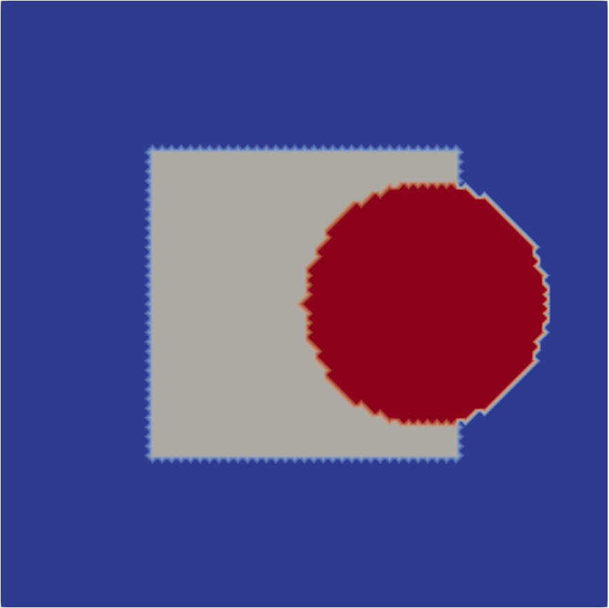
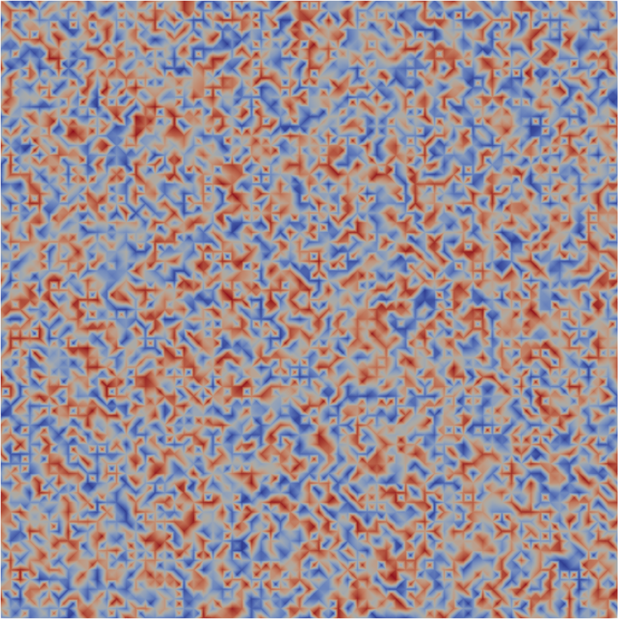
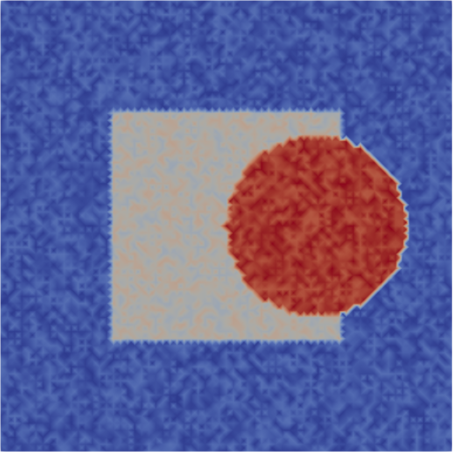
Figure 1. The original image $\tilde{g}_{h}$ (left), the noise $\xi_{h}$ (middle) and the noisy image $g_{h}$ (right).

In all experiments we set $T=0.1$, $\lambda=200$, $\varepsilon=10^{-4}$, $x^{0}_{h}=\tilde{g}_{h}$. The nonlinear algebraic system which corresponds to (9) is solved using a simple fixed-point iterative scheme with tolerance $10^{-4}$. If not mentioned otherwise we use the time step $\tau=10^{-3}$, the mesh size $h=2^{-6}$ and $\sigma=1$.

The time-evolution of the discrete energy functional $\mathcal{J}_{\varepsilon}$ for one realization of the space-time noise $W_{h}$ is displayed in Figure 2 (left); $\mathrm{P1}$ denotes the solution with the conforming finite element approximation and $\mathrm{CR}$ denotes the non-conforming approximation, $\mathrm{h7}$, $\mathrm{h8}$ respectively denote the solution with mesh size $h=2^{-7},\,\,2^{-8}$ and $det$ stands for the deterministic solution with $\sigma=0$. The evolution of the approximation error of the original image $\tilde{g}_{h}$ is displayed in Figure 2 (left). We make the following observations for the conforming finite element method: the approximation error for $\sigma=0$ improves with decreasing mesh size, and the approximation error of the stochastic problem oscillates around the error of the deterministic counterpart. For the non-conforming approximation we measure the approximation error of the projected discrete solution $\Pi_{h}^{0}X_{\varepsilon,h}^{i}$, $i=1,\dots$, where $\Pi_{h}^{0}$ is the projection onto piecewise constant functions on $\mathcal{T}_{h}$, see Figure 3 where we also display the solution of the conforming finite element scheme. As expected, cf. [3], on the same mesh with $\sigma=0$ the non-conforming finite element method yields a better approximation of the original image then the conforming method. The non-conforming approximation requires roughly $3\times$ more degrees of freedom than the conforming one but the approximation is still comparable to the conforming method with smaller mesh size $h=2^{-7}$ (which involves $4\times$ more degrees of freedom than the approximation with $h=2^{-6}$). Nevertheless, we also observe that the non-conforming approximation is more sensitive to the noise. For comparison in Figure 4 we display the piecewise constant projections of the solutions computed with the conforming scheme with $h=2^{-6}$ and $h=2^{-8}$.

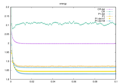
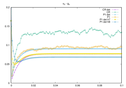
Figure 2. Evolution of the discrete energy (left) and evolution of the discrete error $t_{i}\rightarrow\frac{\lambda}{2}\|X_{\varepsilon,h}^{i}-\tilde{g}_{h}\|^{2}$ (right).

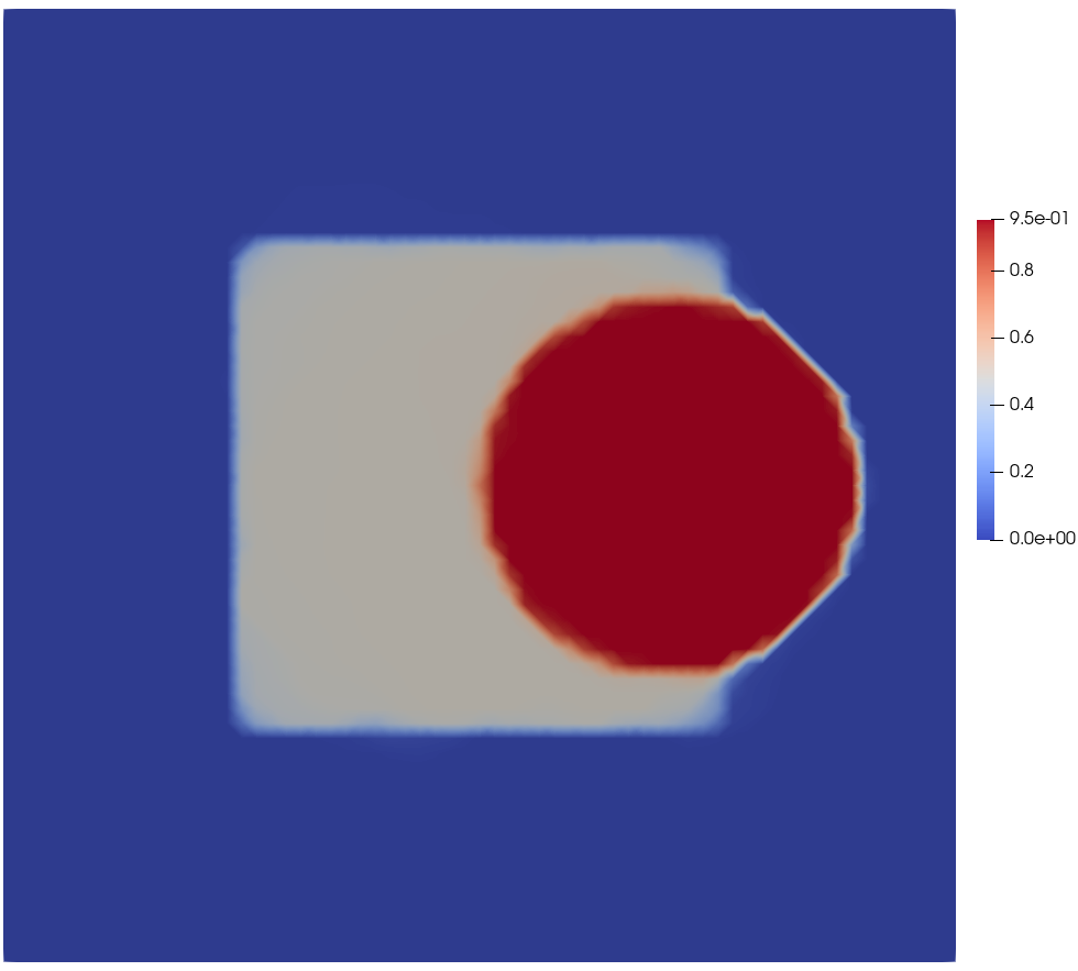
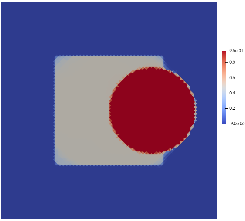
Figure 3. Solution computed with the conforming finite element scheme (left) and the projected solution of the non-conforming finite element scheme (right).

Figure 4. Projected solution of the conforming finite element scheme with $\sigma=0$ for $h=2^{-6}$ (left) and $h=2^{-8}$ (right) at $T=0.1$.

Appendix A Proofs of the results from Section 5

A.1. Proof of Theorem 3

The proof is analogous to that of the generalized Arzela-Ascoli theorem e.g. [16, Theorem 7.6]. Denote by $\tau_{\mathbf{p}}$ the topology of pointwise convergence on $Y^{[0,T]}$. Apparently, $\tau_{\mathbf{p}}\subseteq\tau_{\mathbf{u}}$. Basically, (i) yields that $\overline{M}^{\tau_{\mathbf{p}}}$ is compact in $Y^{[0,T]}$ by the Tychonoff theorem, and the traces of $\tau_{\mathbf{p}}$ and $\tau_{\mathbf{u}}$ coincide on $\overline{M}^{\tau_{\mathbf{p}}}$ by (ii). To see the latter, fix an absolutely convex neighbourhood of zero $O$ and get $\delta>0$ and $m\in\mathbb{N}$ from (ii). Let $D$ be a finite subset of $(T\mathbb{Q})\cap[0,T]$ that contains all $t^{n}_{j}$ for $0\leq j\leq n\leq m$, let $D$ intersect each non-empty intersection $(t^{k}_{i-1},t^{k}_{i})\cap(t^{l}_{j-1},t^{l}_{j})$ whenever $1\leq i\leq k\leq m$, $1\leq j\leq l\leq m$, and let $D$ be a $\delta$-net in $(t^{k}_{i-1},t^{k}_{i})$ for every $1\leq i\leq k\leq m$. With these preparations, if $f,g\in M$ are such that $f(r)-g(r)\in O$ for every $r\in D$ then $f(t)-g(t)\in 3O$ for every $t\in[0,T]$. Thus, if $f,g\in\overline{M}^{\tau_{\mathbf{p}}}$ are such that $f(r)-g(r)\in O$ for every $r\in D$ then $f(t)-g(t)\in 3\overline{O}$ for every $t\in[0,T]$. In particular, (ii) yields that $\tau_{\mathbf{p}}$ is stronger than $\tau_{\mathbf{u}}$ on $\overline{M}^{\tau_{\mathbf{p}}}$. But since $\tau_{\mathbf{p}}$ is weaker than $\tau_{\mathbf{u}}$, the topologies coincide on $\overline{M}^{\tau_{\mathbf{p}}}$. Now (ii) also yields

(30) $$\overline{M}^{\tau_{\mathbf{p}}}=\bigcap_{n=1}^{\infty}\left\{\overline{M_{n}^{\uparrow}}^{\tau_{\mathbf{p}}}\cup\bigcup_{m=1}^{n-1}\overline{M\cap Q_{m}}^{\tau_{\mathbf{p}}}\right\}\subseteq Q_{\infty}\cup\bigcap_{n=1}^{\infty}\overline{M_{n}^{\uparrow}}^{\tau_{\mathbf{p}}}\subseteq Q_{\infty}\cup C([0,T];Y)=Q_{c}.$$

The implication (iii) $\Rightarrow$ (i) is obvious and one gets (iii) $\Rightarrow$ (ii) by contradiction.

To prove (iii) $\Rightarrow$ (iv) and the assertion in Remark 9, we are going to use only the fact that $f(s+)$ and $f(t-)$ exist for every $0\leq s<t\leq T$ and every $f$ in $\overline{M}$. For let $K$ be the closure of $M$ and define

$$R=\left\{f(t-),f(t),f(t+):\,t\in[0,T],\,f\in K\right\}$$

where $f(0-):=f(0)$ and $f(T_{+}):=f(T)$. The definition of $R$ is correct since we know by (30) that $K\subseteq Q_{\infty}\cup C([0,T];Y)$ if (iii) holds, or we refer to Remark 7. Let us prove that $R$ is compact in $Y$. For let $\mathcal{U}$ be an ultrafilter in $R$ and define

$$S_{U}=\{(t,f)\in[0,T]\times C:\,\{f(t-),f(t),f(t+)\}\cap U\neq\emptyset\}.$$

Then $\{S_{U}:\,U\in\mathcal{U}\}$ is a basis of a filter in the compact space $[0,T]\times K$, and therefore it converges to some $(s,g)\in[0,T]\times K$. We conclude that

$$\left[\left(g(s-)+O\right)\cup\left(g(s)+O\right)\cup\left(g(s+)+O\right)\right]\cap U\neq\emptyset$$

holds for every $U\in\mathcal{U}$ and every neighbourhood $O$ of zero in $Y$. Since $\mathcal{U}$ is an ultrafilter,

$$\left[\left(g(s-)+O\right)\cup\left(g(s)+O\right)\cup\left(g(s+)+O\right)\right]\cap R\in\mathcal{U}$$

and so $\mathcal{U}$ converges to one of the elements in the set $\{g(s-),g(s),g(s+)\}$.

A.2. Proof of Corollary 1

Say that $f$ takes values in some compact $K$ for every $f\in M$, let $\{[|\cdot|_{n}<1]:\,n\in\mathbb{N}\}$ be a basis of absolutely convex open neighbourhoods of zero in the compact set

$$C=\bigcup_{\max\,\{|a|,|b|\}\leq 1}(aK+bK)$$

for some continuous pseudonorms $|\cdot|_{n}$ on $Y$ and define

$$d(y_{1},y_{2})=\sum_{n=1}^{\infty}2^{-n}\min\,\{1,|y_{1}-y_{2}|_{n}\},\qquad y_{1},y_{2}\in Y.$$

Then

(31) $$D(f,g)=\sup\,\{d(f(t),g(t)):\,t\in[0,T]\},\qquad f,g\in Q([0,T];Y)$$

metrizes the topology on $M$.

A.3. Proof of Corollary 2

It suffices to prove the assertion for compact sets $M$ in $Q_{c}([0,T];Y)$. The mapping $f\mapsto D(f,g)$ is $\mathcal{Y}_{T}$-measurable for every $g\in Q([0,T];Y)$ by Remark 6, hence the traces of $\mathscr{B}(Q([0,T];Y))$ and $\mathcal{Y}_{T}$ coincide on $M$ as $(M,D)$ is a separable metric space by Corollary 1. Now it suffices to prove that $M$ itself belongs to $\mathcal{Y}_{T}$. According to Theorem 3, there exist $\{m_{n}:\,n\in\mathbb{N}\}\subseteq\mathbb{N}$ and $\{\delta_{n}:\,n\in\mathbb{N}\}\subseteq(0,\infty)$ such that $M\subseteq R$ where

$$R=\left[\bigcap_{t\in[0,T]}\pi_{t}^{-1}[K]\right]\cap\bigcap_{n=1}^{\infty}\left\{\left[\bigcup_{j=1}^{m_{n}}Q_{j}\right]\cup\left[\bigcap_{|t-s|\leq\delta_{n}}\{f:\,|f(t)-f(s)|_{n}\leq 1\}\right]\right\},$$

and $K$ and $\{|\cdot|_{n}\}$ are the same as in the proof of Corollary 1. But $R$ is closed (as an intersection of closed sets), relatively compact in $Q_{c}([0,T];Y)$ by Theorem 3 (hence compact), and $\mathcal{Y}_{T}$-measurable as

$$R=\left[\bigcap_{t\in D_{T}}\pi_{t}^{-1}[K]\right]\cap\bigcap_{n=1}^{\infty}\left\{\left[\bigcup_{j=1}^{m_{n}}Q_{j}\right]\cup\left[\bigcap_{t,s\in D_{T},\,|t-s|\leq\delta_{n}}\{f:\,|f(t)-f(s)|_{n}\leq 1\}\right]\right\}$$

where $D_{T}=(T\mathbb{Q})\cap[0,T]$. Thus the trace of $\mathscr{B}(Q([0,T];Y))$ on $R$ is a subset of $\mathcal{Y}_{T}$ and, in particular, $M\in\mathcal{Y}_{T}$.

A.4. Proof of Proposition 1

It suffices to prove the first assertion for $F_{n}$ and $F$ real-valued (otherwise compose theses functions with $x\mapsto\min\,\{x,m\}$ and then let $m\to\infty$). If $t\in(0,\infty)$ then set $R=(-\infty,t]$, and we have, for every $r\in(0,1)$,

$$\mu_{n}(F_{n}\in R)\leq r+\mu_{n}\left(\overline{\bigcup_{k=m}^{\infty}[F_{k}\in R]\cap K_{r,k}}\right),\qquad m\leq n,$$

so

$$\limsup\mu_{n}(F_{n}\in R) \leq r+\mu\left(\bigcap_{m=1}^{\infty}\overline{\bigcup_{k=m}^{\infty}[F_{k}\in R]\cap K_{r,k}}\right)$$

$$\leq r+\mu(F\in R)+\mu^{*}(D_{r})$$

by the classical Portmanteau theorem, cf. [8, Corollary 8.2.10], hence

$$\liminf\mu_{n}(F_{n}>t)\geq\mu(F>t)$$

and therefore

$$\int_{X}F\mathrm{d}\mu=\int_{0}^{\infty}\mu(F>t)\,\mathrm{d}t\leq\liminf\int_{0}^{\infty}\mu_{n}(F_{n}>t)\,\mathrm{d}t=\liminf\int_{X}F_{n}\,\mathrm{d}\mu$$

by the Fatou lemma. The second part of the proof is analogous but we take any closed set $R$. In this way, we get

$$\limsup\mu_{n}(F_{n}\in R)\leq\mu(F\in R)$$

for every $R$ closed, therefore $\limsup\mu_{n}(F_{n}\in\cdot\,)\Rightarrow\mu(F\in\cdot\,)$. The first part of the proof now yields that $|F|$ is integrable with respect to $\mu$, and we get the claim by the assumption of uniform integrability of $|F_{n}|\,d\mu_{n}$.

Appendix B Bounded variation spaces

Lemma 8.

The functional

$$\mathcal{I}(u)=\sup\,\left\{\int_{\mathcal{O}}u\operatorname{div}\varphi\,\mathrm{d}x:\,\varphi\in C^{\infty}(\mathbb{R}^{d};\mathbb{R}^{d}),\,|\varphi|\leq 1\right\},\qquad u\in\mathbb{L}^{1}$$

satisfies

$$\mathcal{I}(u)=\|\nabla u\|_{\operatorname{TV}(\mathcal{O})}+\int_{\partial\mathcal{O}}{|u|}\,\mathrm{d}x,\qquad\mathrm{for}\,u\in BV(O)$$

and $\mathcal{I}(u)=\infty$ for $u\in\mathbb{L}^{1}\setminus BV(O)$. In particular, $\mathcal{I}$ is lower semicontinuous on $(\mathbb{L}^{1},\operatorname{weak})$ and convex on $BV(\mathcal{O})$ and $\mathcal{J}$ is lower weakly semicontinuous on $\mathbb{L}^{2}$ and convex on $\mathbb{L}^{2}\cap BV(\mathcal{O})$.

Proof.

If $\mathcal{I}(u)<\infty$ then $u\in BV(O)$ e.g. by Proposition 3.6 in [1]. If $u\in BV(O)$ then

$$\int_{\mathcal{O}}u\operatorname{div}\varphi\,\mathrm{d}x=\int_{\partial\mathcal{O}}u(\varphi,\nu)\,\mathrm{d}S-\int_{\mathcal{O}}\varphi\cdot\,\mathrm{d}\,\nabla u,\qquad\varphi\in C^{\infty}(\mathbb{R}^{d};\mathbb{R}^{d})$$

where $\nu$ is the outer normal vector field on $\partial O$ by the integration by parts formula, see e.g. (3.85) in [1], so

$$\mathcal{I}(u)=\sup\,\left\{\int_{\overline{\mathcal{O}}}\varphi\cdot\,\mathrm{d}\,\theta:\,\varphi:\mathbb{R}^{d}\to\mathbb{R}^{d}\text{ Borel measurable},\,|\varphi|\leq 1\right\}\,,$$

by a standard density argument where $\theta=u\nu\mathcal{H}_{d-1}|_{\partial O}-\nabla u$. Hence

$$\mathcal{I}(u)=\|\theta\|_{\operatorname{TV}(\overline{\mathcal{O}})}=\|\nabla u\|_{\operatorname{TV}(\mathcal{O})}+\|u\nu\mathcal{H}_{d-1}\|_{\operatorname{TV}(\partial\mathcal{O})}=\|\nabla u\|_{\operatorname{TV}(\mathcal{O})}+\int_{\partial\mathcal{O}}|u|\,\mathrm{d}S.$$

∎

Remark 12.

There exists a countable subset $\mathcal{H}$ of $C^{\infty}(\mathbb{R}^{d})$ such that

$$\mathcal{I}(u)=\sup\,\left\{\int_{\mathcal{O}}u\phi\,\mathrm{d}x:\,\phi\in\mathcal{H}\right\},\qquad u\in\mathbb{L}^{1}$$

by separability of $\{\operatorname{div}\varphi:\,\varphi\in C^{\infty}(\mathbb{R}^{d};\mathbb{R}^{d}),\,|\varphi|\leq 1\}$ in $C^{\infty}(\mathbb{R}^{d})$.

Appendix C Besov spaces

Lemma 9.

Let $Y$ be a Banach space and let $f:[0,T]\to Y$ be a continuous function linear on every $[t_{i},t_{i+1}]$ for $i=0,\dots,N-1$ and define

$$f_{i,a}=\left[\tau\sum_{j=i}^{N}\|f(t_{j})-f(t_{j-i})\|^{a}\right]^{\frac{1}{a}},\qquad f_{i,\infty}=\max_{i\leq j\leq N}\|f(t_{j})-f(t_{j-i})\|.$$

Then

$$\|f\|_{L^{r}(0,T)}\leq\left[\sum_{i=0}^{N}\tau\|f(t_{i})\|^{r}\right]^{\frac{1}{r}},\qquad\|f\|_{L^{\infty}(0,T)}\leq\,\max_{0\leq i\leq N}\|f(t_{i})\|$$

$$\quad[f]_{B^{s}_{p,q}}\leq\frac{8}{s(1-s)}\left(\sum_{i=1}^{N-1}\tau\frac{f_{i,p}^{q}}{t_{i}^{1+sq}}\right)^{\frac{1}{q}},\quad[f]_{B^{s}_{p,\infty}}\leq 3\max_{1\leq i<N}\frac{f_{i,p}}{t_{i}^{s}}$$

for every $s\in(0,1)$, $p\in[1,\infty]$ and $r,q\in[1,\infty)$.

References

- [1] Luigi Ambrosio, Nicola Fusco, and Diego Pallara. Functions of bounded variation and free discontinuity problems. Oxford Mathematical Monographs. The Clarendon Press, Oxford University Press, New York, 2000.
- [2] V. Barbu and M. Röckner. Stochastic variational inequalities and applications to the total variation flow perturbed by linear multiplicative noise. Arch. Ration. Mech. Anal., 209(3):797–834, 2013.
- [3] S. Bartels. Nonconforming discretizations of convex minimization problems and precise relations to mixed methods. Comput. Math. Appl., 93:214–229, 2021.
- [4] Ľ. Baňas, M. Röckner, and A. Wilke. Convergent numerical approximation of the stochastic total variation flow. Stoch. Partial Differ. Equ. Anal. Comput., 9(2):437–471, 2021.
- [5] Ľ. Baňas, M. Röckner, and A. Wilke. Convergent numerical approximation of the stochastic total variation flow: the higher dimensional case, 2022. preprint.
- [6] Ľ. Baňas, M. Röckner, and A. Wilke. Erratum: ”convergent numerical approximation of the stochastic total variation flow”, 2022. preprint.
- [7] Patrick Billingsley. Convergence of probability measures. Wiley Series in Probability and Statistics: Probability and Statistics. John Wiley & Sons, Inc., New York, second edition, 1999. A Wiley-Interscience Publication.
- [8] V. I. Bogachev. Measure theory. Vol. I, II. Springer-Verlag, Berlin, 2007.
- [9] James H. Bramble, Joseph E. Pasciak, and Olaf Steinbach. On the stability of the projection in . Math. Comp., 71(237):147–156, 2002.
- [10] Dominic Breit, Eduard Feireisl, and Martina Hofmanová. Stochastically forced compressible fluid flows, volume 3 of De Gruyter Series in Applied and Numerical Mathematics. De Gruyter, Berlin, 2018.
- [11] S. C. Brenner and L. R. Scott. The mathematical theory of finite element methods, volume 15 of Texts in Applied Mathematics. Springer, New York, third edition, 2008.
- [12] X. Feng and A. Prohl. Analysis of total variation flow and its finite element approximations. M2AN Math. Model. Numer. Anal., 37(3):533–556, 2003.
- [13] István Gyöngy and Nicolai Krylov. Existence of strong solutions for Itô’s stochastic equations via approximations. Probab. Theory Related Fields, 105(2):143–158, 1996.
- [14] A. Jakubowski. The almost sure Skorokhod representation for subsequences in nonmetric spaces. Teor. Veroyatnost. i Primenen., 42(1):209–216, 1997.
- [15] Ioannis Karatzas and Steven E. Shreve. Brownian motion and stochastic calculus, volume 113 of Graduate Texts in Mathematics. Springer-Verlag, New York, second edition, 1991.
- [16] John L. Kelley. General topology. Graduate Texts in Mathematics, No. 27. Springer-Verlag, New York-Berlin, 1975. Reprint of the 1955 edition [Van Nostrand, Toronto, Ont.].
- [17] M. Ondreját, A. Prohl, and N. Walkington. Numerical approximation of nonlinear SPDE’s, 2020.
- [18] Jacques Simon. Sobolev, Besov and Nikolskiĭ fractional spaces: imbeddings and comparisons for vector valued spaces on an interval. Ann. Mat. Pura Appl. (4), 157:117–148, 1990.