RLFlow: Optimising Neural Network Subgraph Transformation with World Models

Abstract.

Training deep learning models takes an extremely long execution time and consumes large amounts of computing resources. At the same time, recent research proposed systems and compilers that are expected to decrease deep learning models runtime. An effective optimisation methodology in data processing is desirable, and the reduction of compute requirements of deep learning models is the focus of extensive research.

In this paper, we address the neural network sub-graph transformation by exploring reinforcement learning (RL) agents to achieve performance improvement. Our proposed approach RLFlow can learn to perform neural network subgraph transformations, without the need for expertly designed heuristics to achieve a high level of performance.

Recent work has aimed at applying RL to computer systems with some success, especially using model-free RL techniques. Model-based reinforcement learning methods have seen an increased focus in research as they can be used to learn the transition dynamics of the environment; this can be leveraged to train an agent using a hallucinogenic environment such as World Model (WM) (Ha and Schmidhuber, 2018), thereby increasing sample efficiency compared to model-free approaches. WM uses variational auto-encoders and it builds a model of the system and allows exploring the model in an inexpensive way.

In RLFlow, we propose a design for a model-based agent with WM which learns to optimise the architecture of neural networks by performing a sequence of sub-graph transformations to reduce model runtime. We show that our approach can match the state-of-the-art performance on common convolutional networks and outperforms by up to 5% those based on transformer-style architectures

1. Introduction

Recent modern software has key components that are underpinned by machine learning (ML) models, specifically, deep neural networks (DNN). Over the past decade, there has been a focus on developing frameworks that provide tools using which we can design, train and evaluate these deep learning models.

A common internal representation for neural networks inside deep learning frameworks is that of a computation graph; a directed acyclic graph where nodes represent a specific computation and edges the paths where data is transferred. It is a common optimisation practice to support graph substitutions. Frameworks such as TensorFlow (Abadi et al., 2015; Abadi et al., 2016) and PyTorch (Paszke et al., 2019) automatically apply optimisations in an effort to reduce computation resources during inference.

Currently, the majority of optimisations in deep learning frameworks are performed using manually defined heuristics. TensorFlow (Abadi et al., 2015; Abadi et al., 2016), TensorRT (NVIDIA, 2017), and TVM (Chen et al., 2018) perform substitutions to a computation graph by using rule-based strategies. For example, TensorFlow (Abadi et al., 2015; Abadi et al., 2016) uses 155 handwritten optimisations composed of 53,000 lines of C++. While such heuristics are applicable for current architectures, network design is consistently evolving. Therefore, we require consistent innovation to discover and design rules that control the application of optimisations with guarantees that strictly improve efficiency. Such an approach is difficult to scale. Eliminating the need for manual engineering work that is required to design and implement the heuristics for applying optimisations is a primary focus of our work.

Recent work, namely TASO (Jia et al., 2019a), has shown the substitution of the subgraphs by replacing heuristics with an automatic cost-based search. However, such approaches may not fully explore the potential search space due to the lack of forward planning in cost-based optimisation. As a step towards resolving the issue of poor exploration, this work explores the use of reinforcement learning (RL). RL is an area of machine learning in which an agent learns to act optimally, given a state and a suitable reward function, through interactions with an environment.

In this paper, we introduce RLFlow, a deep learning graph optimiser that uses Reinforcement Learning for automating graph substitutions. Specifically, we focus on model-based reinforcement learning that aims to learn a model of the environment in which the agents act. We use an approach called “World Models” (WM), first proposed by Ha et al. (Ha and Schmidhuber, 2018). WM use variational auto-encoders, where at first randomly collected episode rollouts are used as training data to build a compact model, followed by training the compact model with Recurrent Neural Networks (RNN) to predict future steps to maximise the expected cumulative reward of rollouts. When using a WM as a simulated environment, several model evaluations can occur safely in parallel and, especially in systems environments, it overcomes the latency impact of updating system environments.

In this work, the network learns to model the dynamics of sub-graph transformations in a deep learning model as well as the impact on the overall runtime of the model when executed on-device. Further, learning a model of the environment provides important benefits; for example, lookahead planning, low-cost state prediction and faster wall-clock training. We examine the use of world models for learning the environment as well as training a controller inside a world model which removes the need for an expensive, time-consuming computer system to apply the chosen subgraph transformations.

Note that training and inferring on Sequence-to-Sequence (Seq2Seq) (Sutskever et al., 2014) models differ from the usual classification problem, which characterises also for Transformers (Vaswani et al., 2017). One of the focuses of our work in this paper is the applicability of RL based graph transformation over such transformer type of models. Transformers are getting very popular beyond Natural Language Processing (NLP) and it will inevitably expand further.

RLFlow is a graph-net based neural network optimisation as an extension of TASO. The basic idea was to substitute TASO’s cost-based backtracking search and replace it with an RL-based optimisation. This enables it to generalise to large unseen graphs and thus, find better-performing solutions than a backtracking search.

To summarise, our contributions are:

• We designed a model-based RL agent and environment for jointly choosing the optimal substitution and substitution location. Our model-based reinforcement learning approach eliminates the need for human-engineered graph optimisations in machine learning frameworks. We show that our approach can improve model runtime by up to 58% compared to current deep learning frameworks.

• We find a novel transformation of popular DNN architectures previously were unfeasible, where the agent isn’t getting stuck in the greedy cost-based exploration, but rather is able to actually learn what is a good transformation given a context.

• Our approach is especially powerful for transformer-style architectures demonstrating that it outperforms state-of-the-art methods by up to 5%.

• We provide a detailed discussion and analysis of our solution as well as comparison to the state-of-the-art methods in published literature.

• This work, to the best of our knowledge, is the first that has applied model-based reinforcement learning in optimising computation graphs.

2. Background

2.1. Computation graphs for neural networks

There has been a rapid development of various deep learning architectures to solve specific groups of tasks. Common examples include convolutional networks, for a variety of tasks such as object detection and classification. Transformer networks for translation and generation of language. Finally, Recurrent networks have been shown to excel at exploiting long and short term trends in data.

Despite the improvements in the accuracy of machine learning (ML) models, the fundamental building blocks of deep learning models have remained largely unchanged. As the networks become more complex, it also becomes tedious to manually optimise the networks to reduce the execution time on hardware. Therefore, there is extensive work to automatically optimise the models, or alternatively, apply a set of hand-crafted optimisations according to pre-defined rules.

Computation graphs are a way to graphically represent both the individual tensor operations in a model, and the connections (or data-flow) along the edges between nodes in the graph. Figure 1 shows how the expression, $y=\texttt{ReLU}(\mathbf{w}\cdot\mathbf{x}+b)$, can be represented graphically as a computation graph.

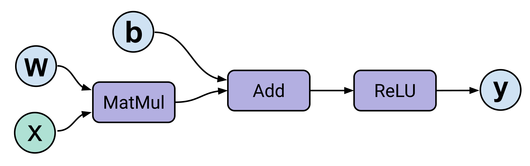
Figure 1. The operations shown in a rounded-rectangular box are the nodes of the computation graph which take an arbitrary number of inputs, performs a computation at the node and produces an output. The circular nodes represent the input nodes for tensors. The directed edges show the flow of tensors through the graph.

Similarly, a neural network model can be converted into a stateful dataflow (computation) graph in this manner. Using a computation graph as an intermediate representation provides two benefits compared to using a raw model definition. First, we can execute the model on any hardware device as the models have a single, uniform representation that can be modified as required. Second, it allows for pre-execution optimisations based on the host device. For example, we may perform different optimisations for executing on a GPU compared to a TPU (Tensor Processing Unit) requires different data layouts and optimisations.

2.2. Reinforcement Learning

Reinforcement learning (RL) is a sub-field of machine learning. Broadly, it aims to compute a control policy such that an agent can maximise its cumulative reward from the environment. Reinforcement Learning has powerful applications in systems environments where a unified model describing the semantics of a system is not available. The agent must itself discover the optimal strategy by a single reward signal.

Formally, RL is a class of learning problem that can be framed as a Markov decision process (MDP) when the MDP that describes the system is not known (Bellman, 1957); they are represented as a 5-tuple $\langle\mathcal{S},\mathcal{A},\mathcal{P}_{a},\mathcal{R}_{a},\rho_{0}\rangle$ where:

• $\mathcal{S}$, is a finite set of valid states

• $\mathcal{A}$, is a finite set of valid actions

• $\mathcal{P}_{a}$, is the transition probability function that an action $a$ in state $s_{t}$ leads to a state $s^{\prime}_{t+1}$

• $\mathcal{R}_{a}$, is the reward function, it returns the reward from the environment after taking an action $a$ between state $s_{t}$ and $s^{\prime}_{t+1}$

• $\rho_{0}$, is the starting state distribution

We aim to compute a policy, denoted by $\pi$, that when given a state $s\in\mathcal{S}$, returns an action $a\in\mathcal{A}$ with the optimisation objective being to find a control policy $\pi^{*}$ that maximises the expected reward from the environment as can be seen in (1). Importantly, we can control the ‘far-sightedness’ of the policy by tuning the discount factor $\gamma\in[0,1)$. As $\gamma$ tends to 1, the policy will consider the rewards further in the future but with a lower weight as the distant expected reward may be an imperfect prediction (Bellman, 1957).

(1) $$\pi^{*}=\operatorname*{arg\,max}_{\pi}~{}\mathbb{E}\left[\sum^{\infty}_{t=0}\gamma^{t}~{}\mathcal{R}_{t}\right]$$

Classic RL problems are formulated as MDPs in which we have a finite state space. However, such methods quickly become inefficient with large state spaces for applications such as Atari (Mnih et al., 2015; Kaiser et al., 2020) and Go (Silver et al., 2018). Therefore, we take advantage of modern deep learning function approximators, such as neural networks, which makes learning the solutions far more efficient in practice. We have seen many successful applications in a wide range of fields, for example, robotic control tasks (OpenAI et al., 2019), data centre power management, device placement (Addanki et al., 2019; Mirhoseini et al., 2018), and playing both perfect and imperfect information games to a super-human level (Silver et al., 2016, 2018). Reinforcement learning excels when applied to environments in which actions may have long-term delayed rewards and inter-connected dependencies that are difficult to learn or model with traditional machine learning techniques.

2.3. Motivation for Model-based RL

Model-free and model-based are the two main approaches to reinforcement learning; with recent work such as (Brown et al., 2020; Kaiser et al., 2020; Robine et al., 2021), the distinction between the two is becoming somewhat nebulous. It is possible to use a hybrid approach that aims to improve the sample efficiency of the agent by training model-free agents directly in the imagined environment.

The primary benefit of model-based RL is that it has greater sample efficiency, meaning, the agent requires in total fewer interactions with the real environment than the model-free counterparts. If we can either provide or learn a model of the environment that enables the agent to plan actions an arbitrary number of steps ahead, the agent selects from a range of trajectories by taking specific actions to maximise its reward. The agent that acts in this “imagined” or “hallucinogenic” environment can be a simple MLP (Ha and Schmidhuber, 2018) to a model-free agent trained using modern algorithms such as PPO (Schulman et al., 2017), A2C (Mnih et al., 2016) or Q-learning (Watkins and Dayan, 1992; Mnih et al., 2015). Further, training an agent in the world model is comparatively cheap, especially in the case of complex systems environments where a single episode can be on the order of hundreds of milliseconds.

Unfortunately, learning a model of the environment is not trivial. The most challenging problem that must be overcome is that if the model is imperfect, the agent may learn to exploit the model’s deficiencies, thus the agent fails to achieve high performance in the real environment. Consequently, learning an invalid world model can lead to the agent performing actions that may be invalid in an environment where not all actions are valid in all states.

Model-based RL approaches have been applied in a range of environments such as board games, video games, systems optimisation and robotics with a high degree of success. Despite the apparent advantages of model-based RL with regards to reduced computation time, model-free reinforcement learning is by far the most popular approach and massive amounts of compute. Typically, the models are trained on distributed clusters of GPUs/TPUs; large amounts of computing resources are required to overcome the sample inefficiency of model-free algorithms.

3. RLFlow

In this section, we introduce RLFlow, a deep learning graph optimiser that uses Reinforcement Learning for automation of graph substitutions, specifically using model-based reinforcement learning by training an agent inside a World Model (Ha and Schmidhuber, 2018) that itself is trained to model the way in which a computation graph is transformed using sub-graph transformations.

3.1. Reinforcement Learning Formulation

3.1.1. System environment

In order to train a reinforcement learning agent, it is necessary that we have access to an environment that, given the current environment state, the agent can take an action. After taking the chosen action, the environment is updated into a new state and the agent receives a reward signal. Typically, one uses a mature environment such as OpenAI Gym (Brockman et al., 2016) or OpenSpiel (Lanctot et al., 2019) as the quality of the environment often has a significant impact on the stability of training. Moreover, using an environment that uses a common interface allows researchers to implement algorithms with ease, and importantly, reproduce results from prior work.

In this work, we designed an environment that follows the OpenAI Gym API standard stepping an environment, that is, we have a function step(action) that accepts a single parameter, the action requested by the agent to be performed in the environment. The step function returns a 4-tuple (next_state, reward, terminal, extra_info). extra_info is a dictionary that can store arbitrary data.

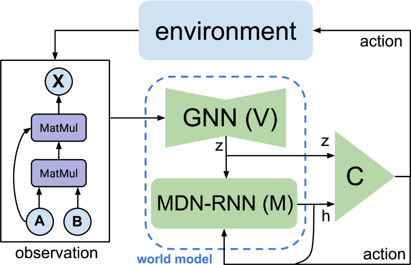
Figure 2. Data flow between components of the system. We select an action given the current state of the imagined environment in the World Model.

We made use of the work by Jia et al. (Jia et al., 2019a) who provided an open-source version of TASO as part of the backend of the environment. We provide a computation graph, as well as the chosen transformation and location tuple to TASO. TASO then applies the requested transformation and returns the newly transformed graph. Further, we use internal TASO functions that calculate estimates of the runtime on the hardware device which we use as our reward signal for training the agent. During our experiments we modified TASO to extract detailed runtime measurements to analyse the rewards using a range of different reward functions—we provide more detail in Section 3.1.4.

3.1.2. Computation Graphs

The first step prior to optimising a deep learning graph is that we must load, or create on-demand, the model in a supported deep learning framework. In our project, we can support any model that can be serialised into the ONNX (Bai et al., 2019) binary format which is an open-source standard for defining the structure of deep learning models. By extension, we can support any deep learning framework that supports serialisation of models into the ONNX format such as TensorFlow (Abadi et al., 2015; Abadi et al., 2016), PyTorch (Paszke et al., 2019) and MXNet (Chen et al., 2015).

Next, we parse the ONNX graph representation by converting all operators into the equivalent TASO tensor representations such that we can modify the graph using the environment API as we described in Section 3.1.1. Although our environment does not support the conversion of all operators defined in the ONNX specification , the majority of the most common operators are supported. Therefore, we still maintain the semantic meaning and structure of the graph. Additionally, after performing optimisations of the graph, we can export the optimised graph directly to an ONNX format.

3.1.3. State-Action space

In this project we modelled the state and action space in accordance with prior research, specifically we referenced work in the similar domain of system optimisation using reinforcement learning. Mirhoseini et al. (Mirhoseini et al., 2018) used hierarchical RL with multiple actions to find the optimal device placement and Addanki et al. (Addanki et al., 2019) that also aided in the choice of input/output graph sizes.

Next, we require two values in order to update the environment. First, we need a select a transformation (which we refer to as an xfer) to apply to the graph. Secondly, the location at which to apply the transformation. As we need to select two actions that are dependent on each other to achieve higher performance, it requires selecting the actions simultaneously.

However, doing so would require a model output of $N\times L$ values, where $N$ is the number of transformations, $L$ is the number of locations. Such an action space is too large to train a model to efficiently predict the correct action. Additionally, after choosing a transformation, we ideally mask the available locations as not all locations can be used to apply any transformation. Therefore, using the same trunk network, we first predict the transformation, apply the location mask for the selected transformation, then predict the location.

We define the action as a 2-value tuple of (xfer_id, location). There is a special case for the xfer_id. When it equals N (the number of available transformations), we consider it the NO-OP action. Therefore, in this special case, we do not modify the graph, rather we terminate the current episode and reset the environment to its initial state.

As explained in the previous section, we used a step-wise approach where at each iteration, we provide a 2-tuple of the transformation and location, to apply in the current state. The updated state from the environment is a 4-tuple consisting of (graph_tuple, xfer_tuples, location_masks, xfer_mask).

xfer_mask refers to a binary mask that indicates the valid and invalid transformations that can be applied to the current computation graph as not every transformation can be applied to every graph. If the current graph has only four possible transformations that can be applied, all other transformations are considered to be invalid. Thus, we return a boolean location mask where only valid transformations are set to 1, or true. This can be used to zero out the model logits of invalid transformations (and thereby actions also) to ensure the agent always selects a valid transformation from the set.

Similarly, for each transformation selected by the agent, there are a number of valid locations where this transformation can be applied. We set a hardcoded, albeit configurable, limit the number of locations to 200 in this work. If the current graph has fewer than 200 possible locations for any given transformation, the remaining are considered invalid. Therefore, we again return a boolean location mask, which is named location_masks in the 4-tuple defined above, which can be used to zero out the model logits where the locations are invalid.

3.1.4. Reward function

The design of a reinforcement learning agent consists of three key elements, the agent, environment and reward function. Most importantly, we require a reward function that captures dynamics of the environment in such a way that we can directly indicate to the agent if we consider the action to be “good” or “bad”. For example, we wish to prevent the agent from performing actions that would be invalid in the environment, therefore, using the reward signal we provide a large negative reward to disincentivise the agent from replicating the behaviour. Conversely, we need to provide a positive reward, that is calculated using the chosen action and its impact on the agent performance.

Selecting optimal actions can be challenging in any deep reinforcement learning system, especially those with either long-term action dependencies or a large number of possible actions in any given state. Importantly, in our environment, the selection of a poor action be impactful on both subsequent action space and the resulting reward generated by the environment. Therefore, we used multiple reward functions to investigate the resulting performance of the agent. First, we used a simple reward function that is commonly used in sequential RL applications:

(2) $$r_{t}=\begin{cases}RT_{t-1}-RT_{t},&\text{if valid action}\\ \text{-}100,&\text{otherwise}\end{cases}$$

Using the reward function defined above, we use the estimated runtime from the prior timestep, $RT_{t-1}$ of the computation graph and the estimated runtime of the current graph, $RT_{t}$, to determine the step-wise, incremental change in graph runtime as the reward. This simple, yet powerful function has the benefit of very low overhead as we only need to store the last runtime. Furthermore, as our primary goal is to reduce the execution time of the graphs, rather than, for example, the system memory, it directly captures our desired metric which we wish to optimise.

Secondly, we instrumented TASO to extract detailed metrics to design a more complex reward function. We used the runtime, FLOPS, memory accesses, and kernel launches to perform experiments to determine if using a combination of the metrics could yield a higher performance RL agent. We defined the modified reward function as shown below. Where $RT_{t}$ is the graph runtime at timestep $t$, $M_{t}$ is the memory accesses at timestep $t$, $\alpha$ and $\beta$ are two hyperparameters for weighting the runtime and memory accesses, respectively.

(3) $$r_{t}=\begin{cases}\alpha(RT_{t-1}-RT_{t})+\beta(M_{t-1}-M_{t}),&\text{if valid action}\\ \text{-}100,&\text{otherwise}\end{cases}$$

We provide further discussion and motivation for our chosen reward functions in Section 4.3 as well as an analysis of the detailed runtime metrics and the impact on graph runtime.

Finally, we note that TASO used a simple method to estimate the runtime of tensor operators that are executed using low-level CUDA APIs and the runtime is averaged over $N$ forward passes. However, this approach to runtime estimation is imperfect as there is a non-negligible variance of the runtime on real hardware and can lead to a poor estimation of the hardware impact. As such, we investigated the use of real runtime measurements during training rather than an estimation of operator runtime. After performing experiments with a modified version of TASO which averages the real runtime over $N$ rounds, we found that it increases the duration of each training step to such a degree that any possible performance improvements achieved using real hardware costs are not worth the trade-off.

3.2. Graph-level optimisation

Performing optimisations at a higher, graph-level means that the resulting graph is—in terms of execution methodology—no different than the original graph before optimisation. By performing graph-level optimisation, we generate a graph representation independent of both the platform and backend. The intermediate representation can be optimised by specialised software for custom hardware accelerators such as GPUs and TPUs.

Next, we define that two computation graphs, $\mathcal{G}$ and $\mathcal{G}^{\prime}$ are semantically equivalent when $\forall\mathcal{I}:\mathcal{G}(\mathcal{I})=\mathcal{G}^{\prime}(\mathcal{I})$ where $\mathcal{I}$ is an arbitrary input tensor. We aim to find the optimal graph $\mathcal{G}^{*}$ that minimises a given cost function, cost$(\mathcal{G})$, by performing a series of transformations to the computation graph at each step, the specific transformation applied does not need to be strictly optimal. In fact, by applying optimisations that reduce graph runtime we further increase the state space for the search; a large state space is preferable in the reinforcement learning domain.

A problem in graph-level optimisation is to define a set of varied, applicable transformations that can be used to optimise the graphs. As previously noted, prior work such as TensorFlow use a manually defined set of transformations and optimise greedily. On the other hand, TASO uses a fully automatic method to generate candidate transformations by performing a hash-based enumeration over all possible DNN operators that result in a semantically equivalent computation graph.

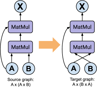
(a) Tensor renaming substitution

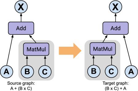
(b) Common subgraph substitution

Figure 3. Two examples of trivial graph substitutions that does not impact the overall runtime of the computation graph. The left sub-figure shows a simple renaming of the tensor inputs. The figure on the right shows that we have a common sub-graph between the source and the target graphs. In both cases we eliminate the duplicates as the hash of the two graphs will be identical.

In this work, we take the same approach as TASO and automatically generate the candidate sub-graphs. We perform this as an offline step as it requires a large amount of computation to both generate and verify the candidate substitution; to place an upper bound on the computation, we limit the input tensor size to a maximum of 4x4x4x4 during the verification process. Following the generation and verification steps, we prune the collection to remove substitutions that are considered trivial and, as such, would not impact runtime. For example, trivial substitutions include input tensor renaming and those with common sub-graphs. We show both techniques diagrammatically in Figure 3(a) and 3(b) respectively.

3.3. World Models

World models, introduced by Ha et al. (Ha and Schmidhuber, 2018), create an imagined model of the true environment by observing states, actions and rewards from the environment and learning to estimate the transitions between states based upon the actions taken. Ha et al. showed that the world models can learn the environment transitions and achieve high performance on visual learning tasks such as CarRacing and VizDoom that exceeds model-free agents. One should note that Ha & Schmidhuber used RGB pixel images as input to a convolutional neural network to generate the latent space embedding. In comparison, we used the latent space produced by the graph neural network using the graph as input. In either case, we aim to learn the world model using the latent space from the environment.

3.3.1. Recurrent Neural Networks

Recurrent Neural networks (RNNs) are a class of architectures in which the connections between the nodes form a directed graph in a temporal sequence (Schuster and Paliwal, 1997). Importantly, as the output of an RNN is deterministic, we use the outputs from the RNN as the parameters for a probabilistic model to insert a controllable level of stochasticity in the output predictions; a method first proposed by Graves (Graves, 2014).

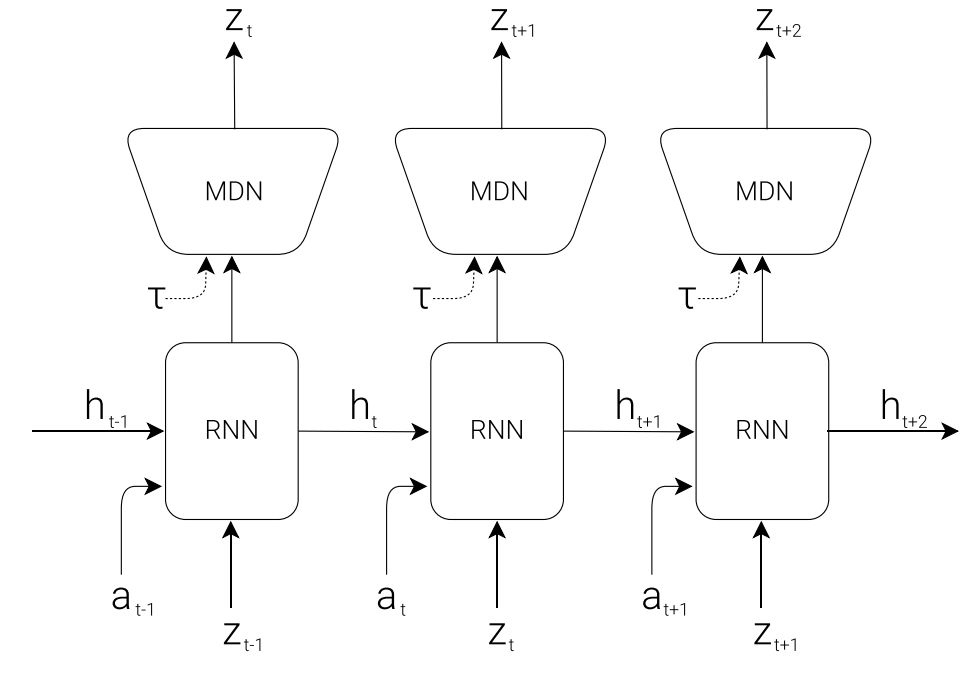
Figure 4. Structure of an unrolled MDN-RNN. The MDN-RNN generates an output which is used as the parameters of a Gaussian mixture distribution. The parameterised GMM is then used to sample the distribution for the vector $z_{t+1}$; the MDN is controlled by the temperature parameter $\tau$. Adapted from (Ha and Schmidhuber, 2018).

A constraint of using RNNs is that they expect a fixed-sized input sequence. In this work, the shape of the latent state tensor and the number of actions available to the agent in a rollout is variable. We use a common approach, called padding, to mitigate this problem by padding the input sequence with zero values until the desired length. After performing inference on the model and retrieving the predicted state, we mask the results based on the input padding to ensure we only use valid predictions to select the next action using the controller.

3.3.2. MDN-RNN

By combining the mixture density and recurrent networks, we can use rollouts of the environment sampled using a random agent to train the combined network, called an MDN-RNN. We use the network to model the distribution $P(z_{t+1}~{}|~{}a_{t},z_{t},h_{t})$, where $z_{t}$ and $z_{t+1}$ is the latent state at the times $t$ and $t+1$ respectively, $a_{t}$ is the action performed at time $t$, and $h_{t}$ is the RNN networks hidden state at time $t$. Figure 4 shows the combination of the RNN and MDN networks and how we calculate the predictions of the next latent state in sequence.

Furthermore, after training the world model, we must train an agent (or controller) to perform actions in the world model that learns to take optimal actions to maximise reward. For inference of the world model, a softmax layer is used that outputs $\pi$ in the form of a categorical probability distribution that we sample under the Gaussian model, often referred to as a Gaussian Mixture Model (GMM), parameterised by $(\mu_{i},\sigma_{i})$.

In Figure 4 we show that one of the inputs to the MDN is $\tau$, the temperature. By altering the temperature, it allows us to control the stochasticity of the agent during the training of the controller. The logits of the RNN that represent the predictions for the values of $\pi$ are divided by the temperature prior to being passed into the softmax function which converts the logits into pseudo-probabilities. We incorporate the temperature, $\tau$, into the function using the following equation.

$$\text{softmax}(\mathbf{x}_{i})=\frac{\exp\left(\frac{x_{i}}{\tau}\right)}{\Sigma_{j}\exp\left(\frac{x_{j}}{\tau}\right)}$$

Typically, the temperature is a real number in the range $\tau\in\left[0,1\right)$, where a value of zero leads to completely deterministic predictions generated by the RNN, whereas larger values introduce a greater amount of stochasticity in predicted values. An increasing value of $\tau$ increases the probability of selecting samples with a lower likelihood; leading to a greater diversity of actions taken by the agent in the environment. Importantly, Ha et al. (Ha and Schmidhuber, 2018) found that having a large temperature can aid in preventing the agent from discovering strategies to exploit in the world model that is not possible true system environment due to an imperfect model.

Modifying the softmax activation function in this way is equivalent to performing knowledge distillation between two models; learnt information is transferred from a large teacher model, or ensemble model, to a smaller model which acts as a student model (Hinton et al., 2015). In both the context of knowledge distillation and training a controller network using the world model, a high temperature will generate softer targets. Specifically, in this work, a higher temperature produces a softer pseudo-probability distribution for $\pi$ in the GMM. Additionally, using soft targets will provide a greater amount of information for the model to be learnt by forcing the model to learn more aggressive policies, thus outputting stochastic predictions that is beneficial to encourage exploring the environment state-action space.

Furthermore, we consider how the world model is trained. For any supervised learning task, we require target data to compare our predictions against, calculate a loss and perform backpropagation to update the weights in the network. To train the world model, we use a random agent. The probability of the agent choosing any action from the set of valid actions is equal. Unlike Ha et al. (Ha and Schmidhuber, 2018) who performed 10,000 rollouts of the environment offline using a random policy to collect the data, we took a different approach.

Rather than generating large rollouts offline, we generated minibatch rollouts using the random agent online and directly used the observations to train the world model. Although this approach reduces the data efficiency as we only use each state observation once, we benefit from removing the need to generate the data prior to training. In systems environments, it is often expensive—in terms of computation time—to step the environment to collect a diverse dataset. Therefore, we found generating short rollouts and training on the minibatch was beneficial without any perceivable impact on performance.

3.4. Action Controller

Finally, we discuss the design of the “controller”, the network/agent that learns to output actions based upon the output from the MDN-RNN world model. Ha and Schmidhuber (Ha and Schmidhuber, 2018) used an evolution-based controller defined as a simple multi-layer-perceptron, $a_{t}=W_{c}[z_{t},h_{t}]+b_{c}$, that accepts the hidden and current states from the recurrent network to predict the next action to be taken. When training the controller inside the world model environment, we no longer have access to the ground truth state nor the reward produced by the real environment. Therefore, we cannot use supervised learning to train the controller.

In (Ha and Schmidhuber, 2018) the authors used an evolutionary algorithm, co-variance matrix adoption evolution strategy (CMA-ES) (Hansen and Ostermeier, 2001; Hansen and Auger, 2014), which optimises the weights of the network based on the reward produced by the world model. Alternatively, recent work by Hafner et al. (Hafner et al., 2020, 2021) has shown to achieve state-of-art results in the Atari environment using an actor-critic method as the controller in the world model. Furthermore, prior work on the application of world models to systems environments has shown one can train a model-free controller inside the world environment (Brown et al., 2020).

4. Evaluation

In this section, we evaluate the aims described at the beginning of the paper. We claimed to use reinforcement learning to perform automated optimisation of deep learning computation graphs. Thus, this evaluation seeks to answer the following questions:

1. Are model-based reinforcement learning methods able to model the transition dynamics of the environment?

2. Are the agent policies able to generalise to unseen states of the same graph to act in accordance to our performance objectives?

3. Do the world models accurately model the reward estimation from the graphs latent state?

4. Are the agents trained in an imagined world model applicable to the real-world environment?

5. Is RL approach more effective for the sequence to sequence models (e.g. Transformers)?

Finally, we conclude with an overall discussion of our findings and their impact.

4.1. Experimental Setup

All experiments presented were performed using a single machine running Ubuntu Linux 18.04 with a 6-core Intel i7-10750H@2.6GHz, 16GB RAM and an NVIDIA GeForce RTX 2070.

To interface with the internal representation of the computation graphs, as previously discussed, we used the open-sourced version of TASO (Jia et al., 2019a) which we modified to extract detailed runtime information. Further, we implemented the reinforcement learning algorithms in TensorFlow (Abadi et al., 2015; Abadi et al., 2016) and utilised the graph_nets package developed by Battaglia et al. (Battaglia et al., 2018) to process our input graphs using the method which we described in Section 3.1.1. The PPO agent was implemented based upon the implementation provided by Schulman et al. (Schulman et al., 2017).

4.2. Graphs Used

Graph	Type	Layers	Unique Layers	Substitutions
InceptionV3	Convolutional	43	12	56
ResNet-18	Convolutional	18	6	40
ResNet-50	Convolutional	50	6	228
SqueezeNet1.1	Convolutional	21	3	288
BERT-Base	Transformer	12	3	80
ViT-Base	Transformer	16	5	60

Table 1. Properties of the six evaluation graphs used in the experiments contained in this chapter. We differentiate the total number of layers in a network from the number of unique layers used in composing the network to provide a more accurate representation of its complexity.

We chose to use six real-world deep learning models to evaluate our project. InceptionV3 (Szegedy et al., 2016) is a common, high-accuracy model for image classification trained on the ImageNet dataset. ResNet-18 & ResNet-50 (He et al., 2016) are also deep convolutional networks that are 18 and 50 layers deep respectively. SqueezeNet (Iandola et al., 2016) is a shallower yet accurate model on the same ImageNet dataset. BERT (Devlin et al., 2019) is a recently introduced large transformer network that has been to improve Google search results (Nayak, 2019). Finally, ViT, a transformer network specifically designed for computer vision tasks; ViT (Dosovitskiy et al., 2021) has been shown to outperform traditional convolutional networks at image recognition tasks. As these graphs were also used in the evaluation of TASO (Jia et al., 2019a), we can show a direct comparison of the performance between the different approaches.

4.3. Reward functions

As we described in Section 3.1.4, the design of the reward function used in the training of RL agents is a pivotal part of the agent’s architecture. In this section, we analyse our proposed reward functions and their effect on the agent’s convergence.

Furthermore, we collected detailed runtime measurements that were recorded at each step of the training process to analyse the correlation between metrics. We collected metrics such as runtime, FLOPS, memory access and the number of kernel launches. As one may suspect, we found that the estimated runtime and memory accesses have a strong correlation; when the memory access decreases, we see a notable decrease in estimated runtime. Therefore, by providing reward signals to the agent that combine the effect of runtime or memory access, the agent will learn to optimise for both metrics.

Figure 5. Normalised reward of each agent using various reward functions while being trained for 500 epochs. R1 uses the second reward function with tuned parameters, R2 uses new runtime reward, R3 uses $\alpha=0.1,\beta=0.9$, R4 uses $\alpha=0.5,\beta=0.5$ and finally, R5 uses incremental runtime improvement.

Figure 5 shows the effect on the convergence of model-free RL agents while training on the BERT graph using various reward functions. Significantly, using the approach of the first reward function (Equation 2) shows that the model-free agent improves at a linear rate as shown by R4 in Figure 5. Alternatively, the second reward function (Equation 3) using tuned hyperparameters of $\alpha$ and $\beta$, shown by R1 in Figure 5, converges the fastest.

However, the rate of convergence does not show the whole picture of the agent’s performance. Despite having a restricted training schedule of 500 epochs, the highest performing agent was trained using reward function R1. It achieved an average runtime improvement of $48.7\pm 3.2\%$. Surprisingly, the second-highest performing agent was the agent using R4, the simplest reward function from the set tested, with a performance of $43.2\pm 2.3\%$.

To find the optimal values of the hyperparameters $\alpha$ and $\beta$ that achieved maximum performance, we performed a grid search for $\alpha$ and $\beta=1-\alpha$ between the values of $[0,1]$ in increments of $0.1$. After training each agent for 500 epochs and evaluating the agent’s performance for five runs, we found that the reward function resulting in the highest performance was using the values $0.8$ and $0.2$ for $\alpha$ and $\beta$ respectively.

4.4. Runtime Performance

Figure 6 shows the runtime of the optimised graphs for the model-based agents trained inside the fully hallucinogenic world model. Each agent was trained inside a world model using rollouts from the respective graph, as described in Section 3.4. We trained the agents for a maximum of 1000 epochs, in mini-batches of 10 epochs. Furthermore, during training of the controller agent network, we used a fixed learning rate for both the policy and value networks.

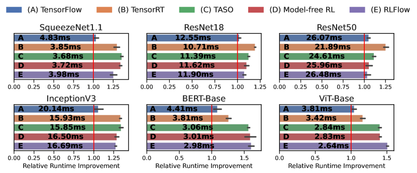
Figure 6. Runtime of optimised graphs using an agent trained using the model-based world model. We also show the baseline results as comparison. The x-axis shows the relative runtime improvement, a higher relative runtime is better. Each experiment was performed five times; we report the mean inference time, and 95% CI through error bars.

Firstly, we note that training the agents on convolutional networks, especially SqueezeNet1.1 and InceptionV3, the model-based agent failed to outperform TASO, although we still decreased the runtime compared to the graph produced by TensorFlow optimisations. Importantly, we observe that the model-based agent outperformed all baseline approaches on the BERT transformer network; we improved the runtime by 54.1% and 7.3% compared to TensorFlow and TASO, respectively. Figure 10 shows the transformations applied by the model-based agent on the test graphs, and compared to TASO, we only apply a single transformation over 20 times—compared to TASO that uses four transformations to produce the optimised graph.

Our model-based agent achieved a similar level of performance on the majority of the tested graphs compared to a model-free agent trained using the real system environment. The model-free agent was trained for 2000 epochs and, by extension, over 4,000,000 interactions with the real environment. Comparatively, the model-based agent performed approximately 1,000,000 interactions with the real environment as the agent did not interact with the real environment while training inside the world model. Therefore, it is evident that by training inside the world model, we improved the sample efficiency of the agent. On the other hand, the agent’s performance decreased compared to the model-free agent in four of the six tested graphs.

Furthermore, an important consideration is the wall-clock time for stepping the environment to a new state, based upon the agent action, when training inside a systems environment. We analysed the time required to perform a single step while training on the ResNet50 graph. We found that stepping the world model (performing inference of the world-model) takes, on average 10ms, whereas stepping the real environment takes on average 850ms. Thus, although the performance of the model-based agent was comparatively lower, our wall-clock time required for training was reduced by a factor of 85x.

Finally, we can observe that RLFlow has higher performance when optimising transformer-based models compared to convolutional networks. A transformer is a deep learning model that adopts the mechanism of attention based on Sequence-to-Sequence (Seq2Seq) architecture (Cho et al., 2014; Sutskever et al., 2014; Vaswani et al., 2017). Seq2Seq models are particularly good at translation, such as Natural Language Processing (NLP), where the sequence of words from one language is translated into an equivalent sequence of words in another language. A popular choice for this type of model is Long-Short-Term-Memory (LSTM) based models. With sequence-dependent data, the LSTM modules can give meaning to the sequence while remembering, or forgetting, the parts it finds important, or unimportant.

Transformers are getting very popular nowadays. Not only in Natural Language Processing (NLP), Vision Transformers (ViTs) (Dosovitskiy et al., 2021) give a good performance on Computer Vision tasks, to the point of outperforming traditional CNNs that have excelled at such tasks. The trend seems to favour Transformers for the majority of NLP tasks. Although, CNNs are still important and are now embedded in GNNs.

4.5. Optimisation Time

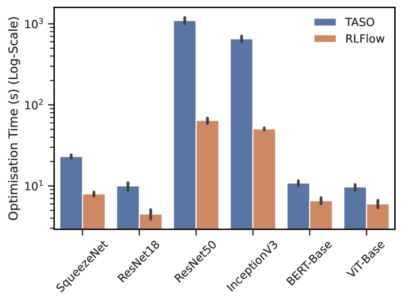
Figure 7. Time required to generate the optimised model using model-based RL and TASO. In all cases, the optimisation time using our proposed approach is lower than that of TASO.

Figure 7 shows the optimisation time required to generate the optimised graph of the tested models. We note that the optimisation time for the model-based agent does not include the time needed to learn the world model, nor training the controller in the environment. The optimisation time is measured as the wall-clock time to perform $n$ agent steps to generate the optimised graph using our RL agents. Thus, although TASO has a longer optimisation time compared to the RL agent, TASO only requires us to perform the cost-based search a single time.

4.6. Memory Usage

Table 2. Relative performance improvement of the graphs when optimised by RLFlow ($\tau=1.0$) compared to TensorFlow

	TensorFlow		RLFlow
	Inf. time (ms)	Mem. usage (GiB)	% Improvement
ResNet18	12.55	1.18	5.2%	1.1%
ResNet50	26.07	2.34	-1.6%	0.6%
InceptionV3	20.14	2.11	17.1%	2.3%
SqueezeNet1.1	4.83	1.14	17.6%	1.8%
BERT-Base	4.41	0.26	32.4%	4.5%
ViT-Base	3.81	0.34	30.7%	3.2%

Table 2 shows the percentage improvement of both the inference time and the memory used for performing inference on the optimised models. Importantly, although we only tasked the agent to optimise for reducing the runtime of the graphs, we observe a secondary effect in a reduction of memory usage by the model of up to 4.5%, compared to TensorFlow. Although this result is not unsurprising, as optimising a model’s architecture leads to a smaller model, based upon the number of trainable parameters. It shows that tasking the agent with reducing runtime does not come at the expense of other resources with strict usage constraints.

4.7. World-model accuracy

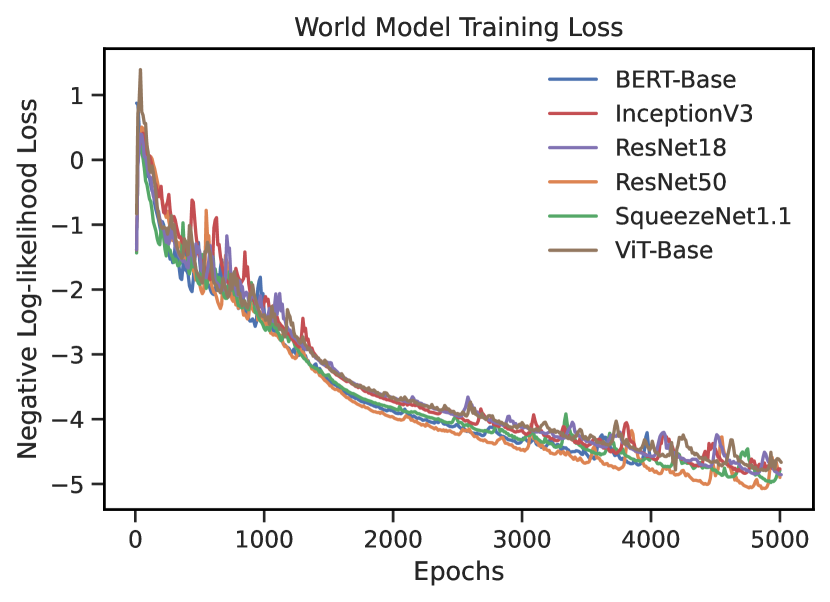
Figure 8. Log-likelihood loss during training on each of the six graphs. The learning rate was decayed over the course of 5000 epochs using a 2nd-degree polynomial decay policy.

The training of the model-based agent is split into two parts. First, we train the world model, the network that learns to simulate the environment dynamics, and secondly, we train the controller network inside the world model. Figure 8 is a plot of the log-likelihood loss for each graph during training of the world model; it shows the convergence of the world model during training after approximately 5000 epochs on all graphs. We used the same hyperparameters for training each world model as well as decaying the learning rate over the course of 5000 epochs with a 2nd-degree polynomial decay policy. We note that despite all the graphs having different architectures, depths and transformation availability, the world model is able to generalise and learn to represent the transformation state transitions accurately after a short period of training. The MDN-RNN is trained with 8 Gaussians and 256 hidden units, all other hyperparameters used in training the MDN-RNN world model are the same as those used by Ha and Schmidhuber (Ha and Schmidhuber, 2018), unless otherwise stated.

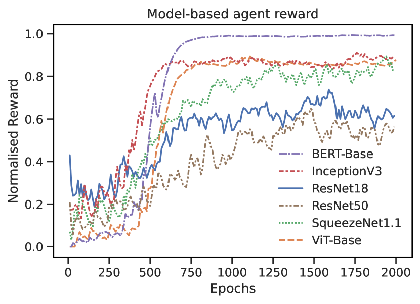
Figure 9. Predicted reward produced by the world model while training the agent inside a the imagined environment. All rewards are normalised into the same range.

Figure 9 shows the reward (decrease in estimated runtime) for each graph as predicted by the world model during training. The tested graphs have a wide range of epoch rewards. We perform min-max normalisation to scale the plots into the same range. This finding also supports the results shown in Figure 6. The agent applies higher-performing optimisations to transformer networks (BERT-Base and ViT-Base) compared to convolutional networks. Notably, for all transformer networks, the optimal strategy is found after approximately 700 epochs.

On the contrary, networks such as ResNet 18/50 are less stable during training with a high epoch to epoch variation in rewards, and we see that the agent struggles to learn an optimal sequence of subgraph transformations to apply.

If we assume that both the model-free and model-based agents should achieve a similar level of performance once trained, the results in Figure 9 shows that the agents trained in the world model are less stable. We hypothesise that there are three factors for such a discrepancy to occur:

• Imperfect world-model reward predictions leading to incorrect (or invalid) actions being performed

• Next state prediction by the world-model generating states that are invalid due to poor generalisation of the model

• Incorrect action mask predictions that would lead to a divergence between the world-model state and real environment state

In an attempt to resolve the issues highlighted above, we performed further experiments that aid in both reducing the variance in reward predictions, as well as stabilise the world model during training to prevent state divergence over time. We performed a temperature sweep of the hyperparameter $\tau$ that is used in training agents inside the world model, shown in Section 4.8.

4.8. Temperature Sweep

Table 3. Temperature sweep of trained model-based agent optimising the BERT network. We show the percentage improvement of the models compared to TensorFlow in the scores produced by the world model and in the real environment. The highest performing model (over five runs) in shown in bold

Temperature	World-model Score	Real Score
0.1	6.67% $\pm$ 0.6%	43.92% $\pm$ 5.1%
0.5	7.75% $\pm$ 0.3%	55.33% $\pm$ 6.7%
0.75	9.10% $\pm$ 0.4%	55.80% $\pm$ 5.2%
1.0	8.85% $\pm$ 1.2%	55.78 $\pm$ 4.0%
1.2	9.91% $\pm$ 0.8%	57.01% $\pm$ 3.9%
1.5	10.20% $\mathbf{\pm}$ 0.6%	58.23% $\mathbf{\pm}$ 3.6%
1.75	9.92% $\pm$ 1.0%	52.07% $\pm$ 5.8%
2.0	9.65% $\pm$ 0.8%	46.12% $\pm$ 5.4%
2.5	10.04% $\pm$ 2.0%	41.14% $\pm$ 10.2%
3.0	10.38% $\pm$ 1.9%	51.32% $\pm$ 7.2%

Table 3 shows the results from performing a temperature sweep in which we used different values of $\tau$ while training the agent in a world model. After training, we evaluated the agent that produced an optimised graph which we evaluated to determine average runtime. The table shows the average reduction in runtime and standard deviation, averaged over five runs, compared to the unoptimised graph. The motivation for using a range of temperatures is that a higher value of $\tau$ leads to softer targets for the agent to predict, thereby improving generalisation. Conversely, a lower value of $\tau$ presents hard targets and thus, when $\tau=1.0$, it is equivalent to using the unmodified mixing weight, $\pi$, of the MDN.

Based upon the results in table 3 from the conducted experiments, we note that the world model agents are stable to temperatures within the range of $\tau=0.5$ to $\tau=1.75$. Although the runtime improvement world-model from the environment is consistently above 6%, we observe a large difference between the predicted runtime improvement and the real environment reward. One approach to producing more accurate reward predictions could be to use a separate reward prediction network.

4.9. Graph transformations

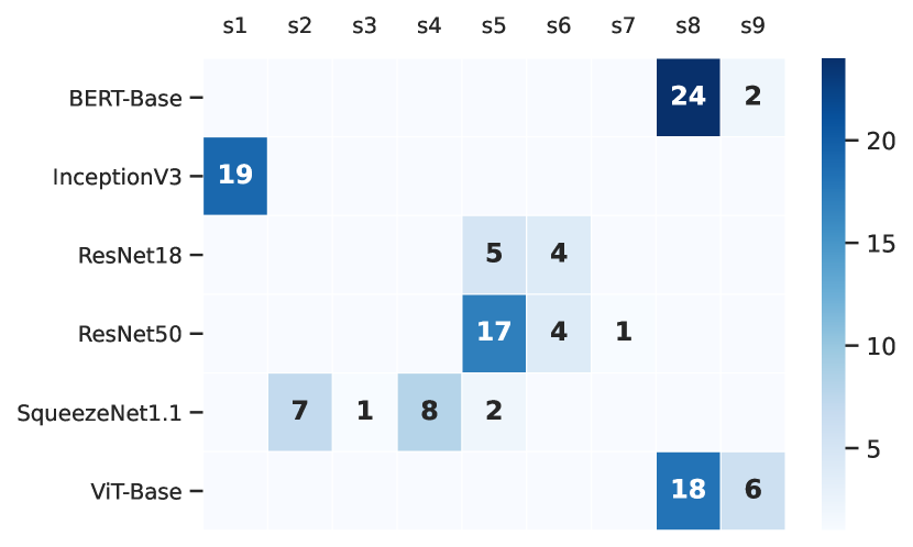
Figure 10. Heatmap showing the transformations applied by the trained controller acting inside the world model. Although there are over 100 possible transformations, we only show the transformations applied onto at least one graph. The counts for each transformation shows the number of times it has been applied. A higher count means that RLFlow was able to find a long sequence of transformations before termination. This can indicate RLFlow has discovered a performant graph via the transformation sequence.

Figure 10 shows a heatmap of the various graph transformations that have been applied by a trained model-based agent during evaluation. Notably, the optimisations applied to the ResNet18/50 graphs apply similar transformations, those targeting the convolutions in the network. The networks are composed of similar convolutional operators, albeit with different depths, and apply analogous transformations. For recurrent networks such as BERT and ViT, we perform relatively few transformations. This is in contrast to transformations performed by TASO that perform four substitutions, in comparison RLFlow that uses only two.

As we can infer from Figure 10, and the results presented in TASO, there is a difference between the two approaches in both the specific transformations and the number of times each was applied. Despite this difference, we found that our method can achieve a similar level of performance in convolutional networks and outperform TASO when optimising transformer-based networks. Primarily, this shows that there are many possible optimisation paths to achieve a performant, highly optimised network architecture.

4.10. Effectiveness on Transformers

Figure 10 shows that RLFlow applies two sub-graph substitutions to the BERT-Base and ViT-Base graphs. These two graphs use a transformer-style architecture that features many repeated layers of Multi-Head Attention, Addition and Normalisation. RLFlow automatically discovered and applied a sub-graph transformation that fused multiple element-wise additions into a single operation that provides a significant reduction in model runtime.

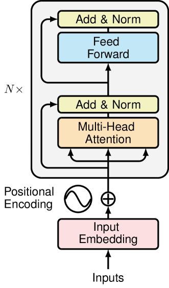
Figure 11. Transformer Encoder architecture. We only show the encoder slice of the whole transformer network. The architecture of ViT (Dosovitskiy et al., 2021) is similar to the transformer architecture presented here, thus, RLFlow can apply the same optimisations that improve model runtime. Adapted from (Vaswani et al., 2017).

Figure 11 shows a simplified version of Transformer encoder block used in state-of-the-art transformer networks. The network contains $N$ repeated blocks, in a similar fashion, the decoder uses repeated blocks of the Transformer Decoder. RLFlow can avoid greedily exploring the search space needlessly when the graph context doesn’t change and instead fuses multiple addition/normalisation operations. In comparison, TASO fails to find the same sub-graph substitution sequence due to its cost-based search ignoring viable substitution sequences. Importantly, using this result, we note that it could be possible to directly implement such rules into the existing heuristics of TensorFlow and PyTorch to automatically improve the performance of transformer-style architectures.

4.11. Summary

In summary, the performance of a cost-directed search is dependent on the neural network architecture. RLFlow’s approach performs better on specific architecture types (such as transformers), compared to convolutional networks (CNNs). The cost-directed search method might be altered and the appropriate optimisation methods for transforming the sub-graphs might be selected.

Recent work, PET (Wang et al., 2021), has shown that CNNs can generally benefit more from partially equivalent transformations compared to the Transformer-based model. The CNN model provides more opportunities for transposing tensor shapes/layouts across dimensions, most of which are partially equivalent transformations, and as the CNNs access data in irregular ways, the approximate transformations are more applicable to achieve higher performance.

The RL agent can consider possible non-equivalent transformations during exploration, therefore, it could achieve better performance on CNN’s. Such a modification only requires adding the partially equivalent transformations to the agent’s action set. However, this is left for future work.

5. Related Work

5.1. Optimisation of computation graphs

To optimise computation graphs we employ a strategy by which we transform an input graph to alter its performance characteristics. Rule-based approaches such as those used in TensorFlow (Abadi et al., 2015; Abadi et al., 2016) and TVM (Chen et al., 2018) use a pre-defined set of transformations that are applied greedily. In addition, recent work, such as (Jia et al., 2019b, a) automatically search for transformations to apply to the input graph with the modification that we allow performance decreasing transformations. Our work is similar as we use the same automated approach to automatically discover and verify the operator transformations in an offline manner, before the optimisation of the models.

5.2. Model-based Reinforcement Learning

Model-based RL is a class of reinforcement learning algorithms in which we aim to learn a model (or use a given model) of the real environment where an agent acts. The work in (Ha and Schmidhuber, 2018) proposed a novel approach to learn a “world model” using recurrent neural networks; we take inspiration from such work and use world models and a policy optimisation algorithm as the controller in the world model. In contrast, alternative approaches have been proposed such as imagination-augmented agents (Racanière et al., 2017) and model-based value estimation for model-free agents (Feinberg et al., 2018). Furthermore, Nagabandi et al. (Nagabandi et al., 2017) proposed a method to combine the sample efficiency of model-based RL and the major benefit of model-free RL, stable performant agents. Our work differs as we use an RNN-based world model to simulate the environment dynamics. Other works such as (Robine et al., 2021; Hafner et al., 2021) build discrete world models and train directly in latent space. Prior work on world models used a variation on a variational auto-encoders (Ha and Schmidhuber, 2018; Hafner et al., 2020) to generate a latent state of the pixel input, instead, we use a graph neural network (Battaglia et al., 2018) to generate a latent representation of the input computation graphs.

5.3. Transformer Networks

Transformer networks are a recent innovation, first described in its popular form by Vaswani et al. (Vaswani et al., 2017). They described a Transformer encoder architecture to solve the Sequence-to-Sequence problem by handling long-range dependencies. Recently, Dosovitskiy et al. (Dosovitskiy et al., 2021) described an approach to encode an RGB image into small patches with positional embedding for use in a Transformer encoder. RLFlow performs well on Transformer-style networks as they share a common architecture. A Transformer encoder is made of repeated blocks of addition, normalisation and multi-head attention operations for which RLFlow can discover and apply sub-graph transformations that results in a high throughput model.

5.4. RL in Computer Systems

Reinforcement Learning in Computer Systems is a relatively recent topic of research. In recent years there has been an increased focus on using model-free RL in a variety of systems environments. For example, in (Mirhoseini et al., 2017, 2018; Addanki et al., 2019; Paliwal et al., 2020), reinforcement learning is used to optimise the placement of machine learning models to improve throughput. In (Brown et al., 2020), model-based RL is used successfully to optimise the selection of bitrate when streaming data across a network. Although prior work has used a cost-directed search or manually defined heuristics, instead, we used model-based RL techniques to optimise the architecture of deep learning models.

6. Conclusion

In this work, we have shown how to apply model-based reinforcement learning techniques to optimise the architecture of neural networks. Our approach uses RL agents to select optimal actions that apply sub-graph transformations to computation graphs to improve on-device runtime. We performed experiments that show RL agents decreased the runtime on all of the six test graphs, each of which had unique properties and architectures. Notably, we provide evidence to support our claim that it is possible to learn a world model of the environment which is sufficiently accurate to enable the end-to-end training of an agent inside a fully imagined world model.

This work has highlighted that the performance of model-based agents trained inside a hallucinogenic is highly dependent on the accuracy of the world model. Inaccuracies in the model, can lead to compounding errors and thus the agent choosing sub-optimal, or invalid, actions that diverge the imagined state from the true environment state. Hence, there are still significant fundamental difficulties in training stable, accurate world models that can simulate the true environment; if one can train such a model by carefully tuning hyperparameters, we can gain substantial benefits through increased sample efficiency and decreased training time.

Finally, we also highlight that RLFlow performs notably well on Transformer-style architectures compared to the state-of-the-art. RLFlow has shown that it is possible to extract further performance from these models through a sequence of sub-graph transformations that combine operations in transformer-encoder blocks—providing up to a 5% decrease in model runtime.

References

- (1)
- Abadi et al. (2015) Martín Abadi, Ashish Agarwal, Paul Barham, Eugene Brevdo, Zhifeng Chen, Craig Citro, Greg S. Corrado, Andy Davis, Jeffrey Dean, Matthieu Devin, Sanjay Ghemawat, Ian Goodfellow, Andrew Harp, Geoffrey Irving, Michael Isard, Rafal Jozefowicz, Yangqing Jia, Lukasz Kaiser, Manjunath Kudlur, Josh Levenberg, Dan Mané, Mike Schuster, Rajat Monga, Sherry Moore, Derek Murray, Chris Olah, Jonathon Shlens, Benoit Steiner, Ilya Sutskever, Kunal Talwar, Paul Tucker, Vincent Vanhoucke, Vijay Vasudevan, Fernanda Viégas, Oriol Vinyals, Pete Warden, Martin Wattenberg, Martin Wicke, Yuan Yu, and Xiaoqiang Zheng. 2015. TensorFlow, Large-scale machine learning on heterogeneous systems. https://github.com/tensorflow/tensorflow. https://doi.org/10.5281/zenodo.4724125
- Abadi et al. (2016) Martín Abadi, Paul Barham, Jianmin Chen, Zhifeng Chen, Andy Davis, Jeffrey Dean, Matthieu Devin, Sanjay Ghemawat, Geoffrey Irving, Michael Isard, Manjunath Kudlur, Josh Levenberg, Rajat Monga, Sherry Moore, Derek G. Murray, Benoit Steiner, Paul Tucker, Vijay Vasudevan, Pete Warden, Martin Wicke, Yuan Yu, and Xiaoqiang Zheng. 2016. TensorFlow: A System for Large-Scale Machine Learning. In 12th USENIX Symposium on Operating Systems Design and Implementation (OSDI 16). USENIX Association, Savannah, GA, 265–283. https://www.usenix.org/conference/osdi16/technical-sessions/presentation/abadi
- Addanki et al. (2019) Ravichandra Addanki, Shaileshh Bojja Venkatakrishnan, Shreyan Gupta, Hongzi Mao, and Mohammad Alizadeh. 2019. Placeto: Learning Generalizable Device Placement Algorithms for Distributed Machine Learning. In Proceedings of the 33rd International Conference on Neural Information Processing Systems. Curran Associates Inc., Red Hook, NY, USA, Article 358, 11 pages.
- Bai et al. (2019) Junjie Bai, Fang Lu, Ke Zhang, et al. 2019. ONNX: Open Neural Network Exchange. https://github.com/onnx/onnx.
- Battaglia et al. (2018) Peter W. Battaglia, Jessica B. Hamrick, Victor Bapst, Alvaro Sanchez-Gonzalez, Vinicius Zambaldi, Mateusz Malinowski, Andrea Tacchetti, David Raposo, Adam Santoro, Ryan Faulkner, Caglar Gulcehre, Francis Song, Andrew Ballard, Justin Gilmer, George Dahl, Ashish Vaswani, Kelsey Allen, Charles Nash, Victoria Langston, Chris Dyer, Nicolas Heess, Daan Wierstra, Pushmeet Kohli, Matt Botvinick, Oriol Vinyals, Yujia Li, and Razvan Pascanu. 2018. Relational inductive biases, deep learning, and graph networks. arXiv:1806.01261 [cs.LG]
- Bellman (1957) Richard Bellman. 1957. A Markovian Decision Process. Journal of Mathematics and Mechanics 6, 5 (1957), 679–684. http://www.jstor.org/stable/24900506
- Brockman et al. (2016) Greg Brockman, Vicki Cheung, Ludwig Pettersson, Jonas Schneider, John Schulman, Jie Tang, and Wojciech Zaremba. 2016. OpenAI Gym. arXiv preprint arXiv:1606.01540 (2016).
- Brown et al. (2020) Harrison Brown, Kai Fricke, and Eiko Yoneki. 2020. World-Models for Bitrate Streaming. Applied Sciences 10, 19 (2020). https://doi.org/10.3390/app10196685
- Chen et al. (2015) Tianqi Chen, Mu Li, Yutian Li, Min Lin, Naiyan Wang, Minjie Wang, Tianjun Xiao, Bing Xu, Chiyuan Zhang, and Zheng Zhang. 2015. MXNet: A Flexible and Efficient Machine Learning Library for Heterogeneous Distributed Systems. arXiv:1512.01274 [cs.DC]
- Chen et al. (2018) Tianqi Chen, Thierry Moreau, Ziheng Jiang, Lianmin Zheng, Eddie Q. Yan, Haichen Shen, Meghan Cowan, Leyuan Wang, Yuwei Hu, Luis Ceze, Carlos Guestrin, and Arvind Krishnamurthy. 2018. TVM: An Automated End-to-End Optimizing Compiler for Deep Learning. In 13th USENIX Symposium on Operating Systems Design and Implementation, OSDI 2018, Carlsbad, CA, USA, October 8-10, 2018, Andrea C. Arpaci-Dusseau and Geoff Voelker (Eds.). USENIX Association, 578–594. https://www.usenix.org/conference/osdi18/presentation/chen
- Cho et al. (2014) Kyunghyun Cho, Bart van Merrienboer, Çaglar Gülçehre, Dzmitry Bahdanau, Fethi Bougares, Holger Schwenk, and Yoshua Bengio. 2014. Learning Phrase Representations using RNN Encoder-Decoder for Statistical Machine Translation. In Proceedings of the 2014 Conference on Empirical Methods in Natural Language Processing, EMNLP 2014, October 25-29, 2014, Doha, Qatar, A meeting of SIGDAT, a Special Interest Group of the ACL, Alessandro Moschitti, Bo Pang, and Walter Daelemans (Eds.). ACL, 1724–1734. https://doi.org/10.3115/v1/d14-1179
- Devlin et al. (2019) Jacob Devlin, Ming-Wei Chang, Kenton Lee, and Kristina Toutanova. 2019. BERT: Pre-training of Deep Bidirectional Transformers for Language Understanding. In Proceedings of the 2019 Conference of the North American Chapter of the Association for Computational Linguistics: Human Language Technologies, NAACL-HLT 2019, Minneapolis, MN, USA, June 2-7, 2019, Volume 1 (Long and Short Papers), Jill Burstein, Christy Doran, and Thamar Solorio (Eds.). Association for Computational Linguistics, 4171–4186. https://doi.org/10.18653/v1/n19-1423
- Dosovitskiy et al. (2021) Alexey Dosovitskiy, Lucas Beyer, Alexander Kolesnikov, Dirk Weissenborn, Xiaohua Zhai, Thomas Unterthiner, Mostafa Dehghani, Matthias Minderer, Georg Heigold, Sylvain Gelly, Jakob Uszkoreit, and Neil Houlsby. 2021. An Image is Worth 16x16 Words: Transformers for Image Recognition at Scale. In 9th International Conference on Learning Representations, ICLR 2021, Virtual Event, Austria, May 3-7, 2021. OpenReview.net. https://openreview.net/forum?id=YicbFdNTTy
- Feinberg et al. (2018) Vladimir Feinberg, Alvin Wan, Ion Stoica, Michael I. Jordan, Joseph E. Gonzalez, and Sergey Levine. 2018. Model-Based Value Estimation for Efficient Model-Free Reinforcement Learning. arXiv:1803.00101 [cs.LG]
- Graves (2014) Alex Graves. 2014. Generating Sequences With Recurrent Neural Networks. arXiv:1308.0850 [cs.NE]
- Ha and Schmidhuber (2018) David Ha and Jürgen Schmidhuber. 2018. Recurrent World Models Facilitate Policy Evolution. In Advances in Neural Information Processing Systems 31: Annual Conference on Neural Information Processing Systems 2018, NeurIPS 2018, December 3-8, 2018, Montréal, Canada, Samy Bengio, Hanna M. Wallach, Hugo Larochelle, Kristen Grauman, Nicolò Cesa-Bianchi, and Roman Garnett (Eds.). 2455–2467. https://proceedings.neurips.cc/paper/2018/hash/2de5d16682c3c35007e4e92982f1a2ba-Abstract.html
- Hafner et al. (2020) Danijar Hafner, Timothy P. Lillicrap, Jimmy Ba, and Mohammad Norouzi. 2020. Dream to Control: Learning Behaviors by Latent Imagination. In 8th International Conference on Learning Representations, ICLR 2020, Addis Ababa, Ethiopia, April 26-30, 2020. OpenReview.net. https://openreview.net/forum?id=S1lOTC4tDS
- Hafner et al. (2021) Danijar Hafner, Timothy P. Lillicrap, Mohammad Norouzi, and Jimmy Ba. 2021. Mastering Atari with Discrete World Models. In 9th International Conference on Learning Representations, ICLR 2021, Virtual Event, Austria, May 3-7, 2021. OpenReview.net. https://openreview.net/forum?id=0oabwyZbOu
- Hansen and Auger (2014) Nikolaus Hansen and Anne Auger. 2014. Principled design of continuous stochastic search: From theory to practice. In Theory and principled methods for the design of metaheuristics. Springer, 145–180.
- Hansen and Ostermeier (2001) Nikolaus Hansen and Andreas Ostermeier. 2001. Completely Derandomized Self-Adaptation in Evolution Strategies. Evol. Comput. 9, 2 (2001), 159–195. https://doi.org/10.1162/106365601750190398
- He et al. (2016) Kaiming He, Xiangyu Zhang, Shaoqing Ren, and Jian Sun. 2016. Deep Residual Learning for Image Recognition. In 2016 IEEE Conference on Computer Vision and Pattern Recognition, CVPR 2016, Las Vegas, NV, USA, June 27-30, 2016. IEEE Computer Society, 770–778. https://doi.org/10.1109/CVPR.2016.90
- Hinton et al. (2015) Geoffrey Hinton, Oriol Vinyals, and Jeffrey Dean. 2015. Distilling the Knowledge in a Neural Network. In NIPS Deep Learning and Representation Learning Workshop. http://arxiv.org/abs/1503.02531
- Iandola et al. (2016) Forrest N. Iandola, Song Han, Matthew W. Moskewicz, Khalid Ashraf, William J. Dally, and Kurt Keutzer. 2016. SqueezeNet: AlexNet-level accuracy with 50x fewer parameters and <0.5MB model size. arXiv:1602.07360 [cs.CV]
- Jia et al. (2019a) Zhihao Jia, Oded Padon, James Thomas, Todd Warszawski, Matei Zaharia, and Alex Aiken. 2019a. TASO: Optimizing Deep Learning Computation with Automatic Generation of Graph Substitutions. In Proceedings of the 27th ACM Symposium on Operating Systems Principles (Huntsville, Ontario, Canada) (SOSP ’19). Association for Computing Machinery, New York, NY, USA, 47–62. https://doi.org/10.1145/3341301.3359630
- Jia et al. (2019b) Zhihao Jia, James Thomas, Tod Warszawski, Mingyu Gao, Matei Zaharia, and Alex Aiken. 2019b. Optimizing dnn computation with relaxed graph substitutions. SysML 2019 (2019).
- Kaiser et al. (2020) Lukasz Kaiser, Mohammad Babaeizadeh, Piotr Milos, Blazej Osinski, Roy H. Campbell, Konrad Czechowski, Dumitru Erhan, Chelsea Finn, Piotr Kozakowski, Sergey Levine, Afroz Mohiuddin, Ryan Sepassi, George Tucker, and Henryk Michalewski. 2020. Model Based Reinforcement Learning for Atari. In 8th International Conference on Learning Representations, ICLR 2020, Addis Ababa, Ethiopia, April 26-30, 2020. OpenReview.net. https://openreview.net/forum?id=S1xCPJHtDB
- Lanctot et al. (2019) Marc Lanctot, Edward Lockhart, Jean-Baptiste Lespiau, Vinicius Zambaldi, Satyaki Upadhyay, Julien Pérolat, Sriram Srinivasan, Finbarr Timbers, Karl Tuyls, Shayegan Omidshafiei, Daniel Hennes, Dustin Morrill, Paul Muller, Timo Ewalds, Ryan Faulkner, János Kramár, Bart De Vylder, Brennan Saeta, James Bradbury, David Ding, Sebastian Borgeaud, Matthew Lai, Julian Schrittwieser, Thomas Anthony, Edward Hughes, Ivo Danihelka, and Jonah Ryan-Davis. 2019. OpenSpiel: A Framework for Reinforcement Learning in Games. CoRR abs/1908.09453 (2019). arXiv:1908.09453 [cs.LG] http://arxiv.org/abs/1908.09453
- Mirhoseini et al. (2018) Azalia Mirhoseini, Anna Goldie, Hieu Pham, Benoit Steiner, Quoc V Le, and Jeff Dean. 2018. A hierarchical model for device placement. In International Conference on Learning Representations.
- Mirhoseini et al. (2017) Azalia Mirhoseini, Hieu Pham, Quoc V Le, Benoit Steiner, Rasmus Larsen, Yuefeng Zhou, Naveen Kumar, Mohammad Norouzi, Samy Bengio, and Jeff Dean. 2017. Device Placement Optimization with Reinforcement Learning. In Proceedings of the 34th International Conference on Machine Learning-Volume 70. JMLR. org, 2430–2439.
- Mnih et al. (2016) Volodymyr Mnih, Adria Puigdomenech Badia, Mehdi Mirza, Alex Graves, Timothy Lillicrap, Tim Harley, David Silver, and Koray Kavukcuoglu. 2016. Asynchronous Methods for Deep Reinforcement Learning. In International Conference on Machine Learning. 1928–1937.
- Mnih et al. (2015) Volodymyr Mnih, Koray Kavukcuoglu, David Silver, Andrei A. Rusu, Joel Veness, Marc G. Bellemare, Alex Graves, Martin A. Riedmiller, Andreas Fidjeland, Georg Ostrovski, Stig Petersen, Charles Beattie, Amir Sadik, Ioannis Antonoglou, Helen King, Dharshan Kumaran, Daan Wierstra, Shane Legg, and Demis Hassabis. 2015. Human-level control through deep reinforcement learning. Nat. 518, 7540 (2015), 529–533. https://doi.org/10.1038/nature14236
- Nagabandi et al. (2017) Anusha Nagabandi, Gregory Kahn, Ronald S. Fearing, and Sergey Levine. 2017. Neural Network Dynamics for Model-Based Deep Reinforcement Learning with Model-Free Fine-Tuning. arXiv:1708.02596 [cs.LG]
- Nayak (2019) Pandu Nayak. 2019. Understanding searches better than ever before. https://blog.google/products/search/search-language-understanding-bert.
- NVIDIA (2017) NVIDIA. 2017. TensorRT: Programmable Inference Accelerator. https://developer.nvidia.com/tensorrt.
- OpenAI et al. (2019) OpenAI, Ilge Akkaya, Marcin Andrychowicz, Maciek Chociej, Mateusz Litwin, Bob McGrew, Arthur Petron, Alex Paino, Matthias Plappert, Glenn Powell, Raphael Ribas, Jonas Schneider, Nikolas Tezak, Jerry Tworek, Peter Welinder, Lilian Weng, Qiming Yuan, Wojciech Zaremba, and Lei Zhang. 2019. Solving Rubik’s Cube with a Robot Hand. arXiv:1910.07113 [cs.LG]
- Paliwal et al. (2020) Aditya Paliwal, Felix Gimeno, Vinod Nair, Yujia Li, Miles Lubin, Pushmeet Kohli, and Oriol Vinyals. 2020. Reinforced Genetic Algorithm Learning for Optimizing Computation Graphs. In 8th International Conference on Learning Representations, ICLR 2020, Addis Ababa, Ethiopia, April 26-30, 2020. OpenReview.net. https://openreview.net/forum?id=rkxDoJBYPB
- Paszke et al. (2019) Adam Paszke, Sam Gross, Francisco Massa, Adam Lerer, James Bradbury, Gregory Chanan, Trevor Killeen, Zeming Lin, Natalia Gimelshein, Luca Antiga, Alban Desmaison, Andreas Kopf, Edward Yang, Zachary DeVito, Martin Raison, Alykhan Tejani, Sasank Chilamkurthy, Benoit Steiner, Lu Fang, Junjie Bai, and Soumith Chintala. 2019. PyTorch: An Imperative Style, High-Performance Deep Learning Library. In Advances in Neural Information Processing Systems 32. Curran Associates, Inc., 8024–8035. http://papers.neurips.cc/paper/9015-pytorch-an-imperative-style-high-performance-deep-learning-library.pdf
- Racanière et al. (2017) Sébastien Racanière, Theophane Weber, David P. Reichert, Lars Buesing, Arthur Guez, Danilo Jimenez Rezende, Adrià Puigdomènech Badia, Oriol Vinyals, Nicolas Heess, Yujia Li, Razvan Pascanu, Peter W. Battaglia, Demis Hassabis, David Silver, and Daan Wierstra. 2017. Imagination-Augmented Agents for Deep Reinforcement Learning. In Advances in Neural Information Processing Systems 30: Annual Conference on Neural Information Processing Systems 2017, December 4-9, 2017, Long Beach, CA, USA, Isabelle Guyon, Ulrike von Luxburg, Samy Bengio, Hanna M. Wallach, Rob Fergus, S. V. N. Vishwanathan, and Roman Garnett (Eds.). 5690–5701. https://proceedings.neurips.cc/paper/2017/hash/9e82757e9a1c12cb710ad680db11f6f1-Abstract.html
- Robine et al. (2021) Jan Robine, Tobias Uelwer, and Stefan Harmeling. 2021. Smaller World Models for Reinforcement Learning. arXiv:2010.05767 [cs.LG]
- Schulman et al. (2017) John Schulman, Filip Wolski, Prafulla Dhariwal, Alec Radford, and Oleg Klimov. 2017. Proximal Policy Optimization Algorithms. arXiv preprint arXiv:1707.06347 (2017).
- Schuster and Paliwal (1997) M. Schuster and K.K. Paliwal. 1997. Bidirectional recurrent neural networks. IEEE Transactions on Signal Processing 45, 11 (1997), 2673–2681. https://doi.org/10.1109/78.650093
- Silver et al. (2016) David Silver, Aja Huang, Chris J Maddison, Arthur Guez, Laurent Sifre, George Van Den Driessche, Julian Schrittwieser, Ioannis Antonoglou, Veda Panneershelvam, Marc Lanctot, et al. 2016. Mastering the game of Go with deep neural networks and tree search. Nature 529, 7587 (2016), 484.
- Silver et al. (2018) David Silver, Thomas Hubert, Julian Schrittwieser, Ioannis Antonoglou, Matthew Lai, Arthur Guez, Marc Lanctot, Laurent Sifre, Dharshan Kumaran, Thore Graepel, Timothy Lillicrap, Karen Simonyan, and Demis Hassabis. 2018. A general reinforcement learning algorithm that masters chess, shogi, and Go through self-play. Science 362, 6419 (2018), 1140–1144. https://doi.org/10.1126/science.aar6404 arXiv:https://www.science.org/doi/pdf/10.1126/science.aar6404
- Sutskever et al. (2014) Ilya Sutskever, Oriol Vinyals, and Quoc V Le. 2014. Sequence to sequence learning with neural networks. In Advances in neural information processing systems. 3104–3112.
- Szegedy et al. (2016) Christian Szegedy, Vincent Vanhoucke, Sergey Ioffe, Jonathon Shlens, and Zbigniew Wojna. 2016. Rethinking the Inception Architecture for Computer Vision. In 2016 IEEE Conference on Computer Vision and Pattern Recognition, CVPR 2016, Las Vegas, NV, USA, June 27-30, 2016. IEEE Computer Society, 2818–2826. https://doi.org/10.1109/CVPR.2016.308
- Vaswani et al. (2017) Ashish Vaswani, Noam Shazeer, Niki Parmar, Jakob Uszkoreit, Llion Jones, Aidan N. Gomez, Lukasz Kaiser, and Illia Polosukhin. 2017. Attention is All you Need. In Advances in Neural Information Processing Systems 30: Annual Conference on Neural Information Processing Systems 2017, December 4-9, 2017, Long Beach, CA, USA, Isabelle Guyon, Ulrike von Luxburg, Samy Bengio, Hanna M. Wallach, Rob Fergus, S. V. N. Vishwanathan, and Roman Garnett (Eds.). 5998–6008. https://proceedings.neurips.cc/paper/2017/hash/3f5ee243547dee91fbd053c1c4a845aa-Abstract.html
- Wang et al. (2021) Haojie Wang, Jidong Zhai, Mingyu Gao, Zixuan Ma, Shizhi Tang, Liyan Zheng, Yuanzhi Li, Kaiyuan Rong, Yuanyong Chen, and Zhihao Jia. 2021. PET: Optimizing Tensor Programs with Partially Equivalent Transformations and Automated Corrections. In 15th USENIX Symposium on Operating Systems Design and Implementation (OSDI 21). 37–54.
- Watkins and Dayan (1992) Christopher JCH Watkins and Peter Dayan. 1992. Q-learning. Machine Learning 8, 3-4 (1992), 279–292.