Kepler and the Behemoth: Three Mini-Neptunes in a 40 Million Year Old Association

Abstract

Stellar positions and velocities from Gaia are yielding a new view of open cluster dispersal. Here we present an analysis of a group of stars spanning Cepheus ($l=100^{\circ}$) to Hercules ($l=40^{\circ}$), hereafter the Cep-Her complex. The group includes four Kepler Objects of Interest: Kepler-1643 b ($R_{\rm p}=2.32\pm 0.13\,R_{\oplus}$, $P=5.3\ {\rm days}$), KOI-7368 b ($R_{\rm p}=2.22\pm 0.12\,R_{\oplus}$, $P=6.8\ {\rm days}$), KOI-7913 Ab ($R_{\rm p}=2.34\pm 0.18\,R_{\oplus}$, $P=24.2\ {\rm days}$), and Kepler-1627 Ab ($R_{\rm p}=3.85\pm 0.11\,R_{\oplus}$, $P=7.2\ {\rm days}$). The latter Neptune-sized planet is in part of the Cep-Her complex called the $\delta$ Lyr cluster (Bouma et al., 2022). Here we focus on the former three systems, which are in other regions of the association. Based on kinematic evidence from Gaia, stellar rotation periods from TESS, and spectroscopy, these three objects are also $\approx$40 million years (Myr) old. More specifically, we find that Kepler-1643 is $46^{+9}_{-7}$ Myr old, based on its membership in a dense sub-cluster of the complex called RSG-5. KOI-7368 and KOI-7913 are $36^{+10}_{-8}$ Myr old, and are in a diffuse region that we call CH-2. Based on the transit shapes and high resolution imaging, all three objects are most likely planets, with false positive probabilities of $6\times 10^{-9}$, $4\times 10^{-3}$, and $1\times 10^{-4}$ for Kepler-1643, KOI-7368, and KOI-7913 respectively. These planets demonstrate that mini-Neptunes with sizes of $\approx$2 Earth radii exist at ages of 40 million years.

1 Introduction

The discovery and characterization of planets younger than a billion years is a major frontier in current exoplanet research. The reason is that the properties of young planets provide benchmarks for studies of planetary evolution. For instance, young planets can inform our understanding of when hot Jupiters arrive on their close-in orbits (Dawson & Johnson, 2018), how the sizes of planets with massive gaseous envelopes evolve (Rizzuto et al., 2020), the timescales for close-in multiplanet systems to fall out of resonance (Izidoro et al., 2017; Arevalo et al., 2022; Goldberg & Batygin, 2022), and whether and how mass-loss explains the radius valley (Lopez et al., 2012; Owen & Wu, 2013; Fulton et al., 2017; Ginzburg et al., 2018; Lee & Connors, 2021).

The discovery of a young planet requires two claims to be true: the planet must exist, and its age must be secured. Spaced-based photometry from K2 and TESS has yielded a number of exemplars for which the planetary evidence comes from transits, and the age is based on either cluster membership (Mann et al., 2017; David et al., 2019; Newton et al., 2019; Bouma et al., 2020; Nardiello et al., 2020) or else on correlates of youth such as stellar rotation, photospheric lithium content, x-ray activity, and emission line strength (Zhou et al., 2021; Hedges et al., 2021).

In this work, we leverage recent analyses of the Gaia data, which have greatly expanded our knowledge of stellar groups (e.g., Cantat-Gaudin et al., 2018; Kounkel & Covey, 2019; Kerr et al., 2021). So far, these analyses have mostly leveraged 3D stellar positions and 2D on-sky tangential velocities. One important result has been the discovery of diffuse streams and tidal tails comparable in stellar mass to the previously known cores of nearby open clusters (Meingast et al., 2019, 2021; Gagné et al., 2021). Even though these streams are spread over tens to hundreds of parsecs, their velocity dispersions can remain coherent at the $\sim$1 km s^-1 level. Internal dynamics and projection effects can also drive them to be much more kinematically diffuse: in the Hyades, stars in the tidal tails are expected to span up to $\pm 40{\rm\,km\,s^{-1}}$ in velocity relative to the cluster center (Jerabkova et al., 2021). The stars in such diffuse regions can be verified to be the same age as the core cluster members through analyses of color–absolute magnitude diagrams (Kounkel & Covey, 2019), stellar rotation periods (Curtis et al., 2019; Bouma et al., 2021), and chemical abundances (Hawkins et al., 2020; Arancibia-Silva et al., 2020). While there are implications for our understanding of star formation and cluster evolution (Dinnbier & Kroupa, 2020), a separate consequence is that we now know the ages of many more stars, including previously known planet hosts.

The prime Kepler mission (Borucki et al., 2010) found most of the currently known transiting exoplanets, and it was conducted before Gaia. It is therefore sensible to revisit the Kepler field, given our new constraints on the stellar ages.

Here, we expand on our earlier study of a $38^{+7}_{-6}$ Myr old Neptune-sized planet in the Kepler field (Kepler-1627 Ab; Bouma et al. 2022). This planet’s age was derived based on its host star’s membership in the $\delta$ Lyr cluster. While our analysis of the cluster focused on the immediate vicinity of Kepler-1627 in order to have a reasonable scope, it became clear that the $\delta$ Lyr cluster seems to also be part of a much larger group of similarly aged stars. This association, which is at an average distance of 330 pc from the Sun, spans Cepheus to Hercules (galactic longitudes, $l$, between 40^∘ and 100^∘), at galactic latitudes between 0^∘ and 20^∘. An assessment of its membership, substructure, and age distribution will be provided as part of the 1 kpc expansion of the SPYGLASS project (R. Kerr et al. in prep), where it is given the name Cep-Her, after the endpoint constellations.

Our focus is on the intersection of the Cep-Her complex with the Kepler field. Cross-matching the stars thought to be in Cep-Her against known Kepler Objects of Interest (KOIs; Thompson et al. 2018) yielded four candidate cluster members: Kepler-1627, Kepler-1643, KOI-7368, and KOI-7913. Given our earlier analysis of Kepler-1627, we focus here on the latter three objects. After analyzing the relevant properties of Cep-Her (Section 2), we derive the stellar properties (Section 3) and validate the planetary nature of each system using a combination of the Kepler photometry and high-resolution imaging (Section 4). We conclude with a discussion of mini-Neptune size evolution, and point out possible directions for future work (Section 5).

2 The Cep-Her Complex

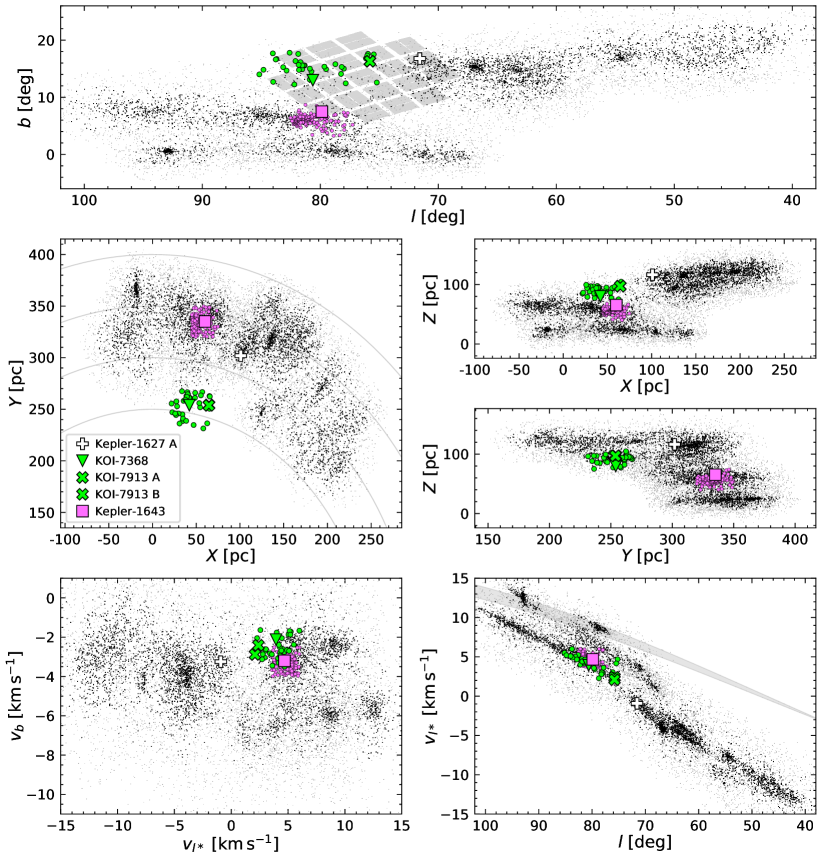
Figure 1: Positions and velocities of candidate members of the Cep-Her complex. Top row: On-sky positions in galactic coordinates. Black points are stars for which group membership is more secure than for gray points. Kepler-1627 is in the outskirts of the $\delta$ Lyr cluster (Bouma et al., 2022), which is centered at $(l,b)\approx(66^{\circ},12^{\circ})$. The Kepler footprint is shown in gray. Middle row: Galactic positions. The Sun is at $(X,Y,Z)=(0,0,20.8)$ pc; lines of constant heliocentric distance are shown between 250 and 400 pc, spaced by 50 pc. Bottom row: Galactic tangential velocities (left) and galactic longitudinal velocity versus galactic longitude (right). The gray band in the lower-right shows the $\pm$1-$\sigma$ projection of the Solar velocity with respect to the local standard of rest (Schönrich et al., 2010). There is a strong spatial and kinematic overlap between Kepler-1643 and RSG-5 (magenta; smaller circles). The local population of candidate young stars around KOI-7368 and KOI-7913 is more diffuse – we call this region “CH-2” (lime-green; larger circles). The selection method for these groups is described in Section 2.2.

2.1 Previous Related Work

Our focus is on a region of the Galaxy 200 to 500 pc from the Sun, above the galactic plane, and spanning galactic longitudes of $40^{\circ}$ to $100^{\circ}$. Two rich clusters in this region are the $\delta$ Lyr cluster (Stephenson, 1959) and RSG-5 (Röser et al., 2016). Each of these clusters was known before Gaia. Their reported ages are between 30 and 60 Myr. Early empirical evidence that these two clusters could be part of a large and more diffuse population was apparent in the Gaia-based photometric analysis of pre-main-sequence stars by Zari et al. (2018, compare their Figures 11 and 13 to our Figure 1). Further kinematic connections and complexity were highlighted by Kounkel & Covey (2019), who included these previously known groups in the larger structures dubbed “Theia 73” and “Theia 96”. The connection made by Kounkel & Covey (2019) between the previously known open clusters and the other groups in the region was made as part of an unsupervised clustering analysis of the Gaia DR2 positions and on-sky velocities with a subsequent manual “stitching” step. Their results support the idea that there is an overdensity of 30 to 60 Myr old stars in this region of the Galaxy. Kerr et al. (2021), in a volume-limited analysis of the Gaia DR2 point-source catalog out to one third of a kiloparsec, identified three of the nearest sub-populations of Cep-Her, dubbed “Cepheus-Cygnus”, “Lyra”, and “Cerberus”. Kerr et al. (2021) reported ages for each of these subgroups between 30 and 35 Myr.

2.2 Member Selection

The possibility that the $\delta$ Lyr cluster, RSG-5, and the sub-populations identified by Kerr et al. (2021) share a common origin has yet to be fully substantiated, but preliminary clustering results from the 1 kpc SPYGLASS analysis (R. Kerr et al. in prep) suggest the presence of contiguous stellar populations connecting each of these groups in both space and velocity coordinates. In other words, the stars appear to be comoving, though with a continuous gradient in velocity as a function of position. The lower panels of Figure 1 show this in detail, where $v_{b}$ is the distance-corrected proper motion in the direction of increasing galactic latitude, and $v_{l^{*}}=v_{l}\cos b$ is the distance-corrected proper motion in the direction of increasing galactic longitude after accounting for the local tangent plane correction. Some, but not all, of the gradient in the $v_{l^{*}}$ vs. $l$ plane can be understood through a projection effect stemming from the Sun’s motion with respect to the local standard of rest (see also Figure 11 by Zari et al. 2018). In this work, our primary interest in this region of sky stems from the fact that a portion of it was observed by Kepler (Figure 1, top panel). To further explore this sub-population, we select candidate Cep-Her members through four steps, the first three being identical to those described in Section 3 of Kerr et al. (2021). We briefly summarize them here.

The first step is to select stars that are photometrically distinct from the field star population based on Gaia EDR3 magnitudes $\{G,G_{\rm RP},G_{\rm BP}\}$, parallaxes and auxiliary reddening estimates (Lallement et al., 2019). This step yielded 1,097 stars with high-quality photometry and astrometry. These stars are either pre-main-sequence K and M dwarfs due to their long contraction timescales, or massive stars near the zero-age main sequence due to their rapid evolutionary timescales.

The second step is to perform an unsupervised HDBSCAN clustering on the photometrically selected population (Campello et al., 2015; McInnes et al., 2017). The parameters we use in the clustering are $\{X,Y,Z,cv_{b},cv_{l^{*}}\}$, where $c$ is the size-velocity corrective factor, which is taken as $c=6\,{\rm pc/km\,s}^{-1}$ to ensure that the spatial and velocity scales have identical standard deviations. Positions are computed assuming the astropy v4.0 coordinate standard (Astropy Collaboration et al., 2018). As input parameters to HDBSCAN, we set the minimum $\epsilon$ threshold past which clusters cannot be fragmented as $25$ pc in physical space, and $25/c$  km s^-1 in velocity. The minimum cluster size $N$ is set to 10, as is $k$, the parameter used to define the “core distance” density metric. Core distance is the distance to the $k^{\rm th}$ nearest star, and therefore $k$ acts as a smoothing parameter, where a larger value reduces the influence of local overdensities smaller than the scale that interests us.

The unsupervised clustering in this case yielded 8 distinct subgroups. These groups are then used as the “seed” populations, in which the stellar members each have their own individually-assigned distances to their tenth-nearest photometrically-young neighbor. Using those distances, we search the entire Gaia EDR3 point source catalog for stars that fall within each star’s 10^th nearest-neighbor distance. This third step yields stars that are spatially and kinematically close to the photometrically young stars, but which cannot be identified as young based on their positions in the color–absolute magnitude diagram.

The outcome of the analysis up to the point of the third step is shown in Figure 1. To enable a selection cut that filters out field-star contaminants, we also compute a weight metric, $D$, defined such that the group member with the smallest core distance has $D=1$, the group member with the greatest core distance has $D=0$, and the weight $D$ scales linearly between the two extremes. After applying a set of quality cuts on the astrometry and photometry this procedure yields a distribution of weights $D$ that is well described by a log-normal distribution with $\log_{10}\mathcal{N}(-1.55,0.61)$. To visualize the results, in Figure 1 we show 12,436 objects with $D>0.02$ as gray points, and 4,763 objects with $D>0.10$ as black points. These thresholds were selected visually based on the apparent purity with which they yielded pre-main-sequence stars on a color–absolute magnitude diagram. The $\delta$ Lyr cluster is visible at $(l,b)=(68^{\circ},15^{\circ}$) and $(v_{l^{*}},v_{b})=(-4.5,-4){\rm\,km\,s^{-1}}$. RSG-5 is visible at $(l,b)=(83^{\circ},6^{\circ})$, $(v_{l^{*}},v_{b})=(5.5,-3.5){\rm\,km\,s^{-1}}$. Most of the other subclusters, including in Cep-Cyg ($l,b=90^{\circ},7^{\circ}$) and Cerberus ($l,b=48^{\circ},18^{\circ}$) are too small or dispersed to have previously been analyzed in great detail.

Our fourth and final step was to cross-match the candidate Cep-Her member list against all known Kepler Objects of Interest. We used the Cumulative KOI table from the NASA Exoplanet Archive from 27 March 2022, and also compared against the q1_q17_dr25 table (Thompson et al., 2018). From the candidate members with weights exceeding 0.02, this yielded 11 known false positives, 6 confirmed planets, and 8 candidate planets (see Appendix A). To determine whether these objects were potentially consistent with being i) planets, and ii) $\lesssim 10^{8}$ years old, we inspected the Kepler data validation reports and Robovetter classifications. Youth was assessed based on the presence of rotational modulation at the expected period and amplitude for stars at least as young as the Pleiades (e.g., Rebull et al., 2020). Planetary status was assessed through the Robovetter flags, and by requiring non-grazing transits with ${\rm S/N}>10$. Four objects passed both cuts: Kepler-1627, Kepler-1643, KOI-7368, and KOI-7913.

Figure 1 shows the positions of these KOIs along various projections. Kepler-1643 is near the core RSG-5 population both spatially and kinematically. KOI-7368 and KOI-7913 are in a diffuse region $\approx$40 pc above RSG-5 in $Z$ and $\approx$100 pc closer to the Sun in $Y$. In tangential galactic velocity space, there is some kinematic overlap between the region containing the latter two KOIs and the main RSG-5 group.

We define two sets of stars in the local vicinity of our objects of interest. For candidate RSG-5 members near Kepler-1643, we require:

$$X/{\rm pc} \in[45,75]$$

$$Y/{\rm pc} \in[320,350]$$

$$Z/{\rm pc} \in[40,80]$$

$$v_{b}/{\rm km\,s^{-1}} \in[-4,-2.5]$$

$$v_{l^{*}}/{\rm km\,s^{-1}} \in[3.5,6],$$

though RSG-5 does have a greater spatial extent toward smaller $X$ (Figure 1, middle panels). For the diffuse stars near KOI-7368 and KOI-7913, we require

$$X/{\rm pc} \in[20,70]$$

$$Y/{\rm pc} \in[230,270]$$

$$Z/{\rm pc} \in[75,105]$$

$$v_{b}/{\rm km\,s^{-1}} \in[-3.5,-1.5]$$

$$v_{l^{*}}/{\rm km\,s^{-1}} \in[2,6]$$

and we call this latter set of stars “CH-2”, using the preliminary Cep-Her (CH) subgroup identifier from R. Kerr et al. (in prep). These cuts yielded 173 candidate RSG-5 members, and 37 candidate CH-2 members. These stars are listed in Appendix A, as is the set of Cep-Her candidates that was observed by Kepler.

2.3 The Cluster’s Age

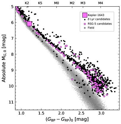
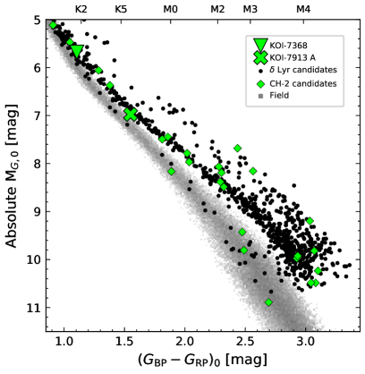
(a)

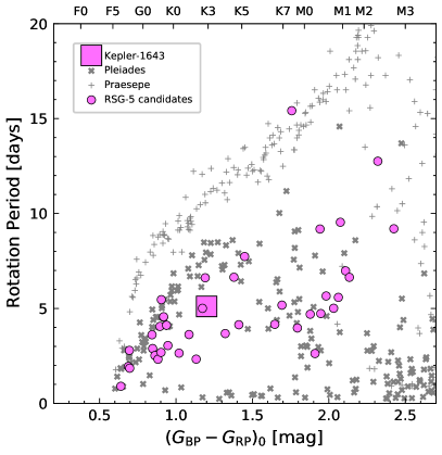
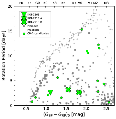
(b)

Figure 2: Age-diagnostic diagrams from the stellar groups near Kepler-1643, KOI-7368, and KOI-7913. Top row: Color–absolute magnitude diagram of candidate Cep-Her members, plotted over candidate members of the $\delta$ Lyr cluster ($\approx 38$ Myr; Bouma et al. 2022) and the Gaia EDR3 Catalog of Nearby Stars (gray background). The left and right columns shows stars in RSG-5 and CH-2, respectively. The range of colors is truncated to emphasize the pre-main-sequence; approximate spectral types are shown on the upper axes. Stars that fall far below the cluster sequences are field interlopers. Bottom row: TESS and ZTF-derived stellar rotation periods, with the Pleiades ($\approx 112$ Myr) and Praesepe ($\approx 650$ Myr) shown for reference (Rebull et al., 2016; Douglas et al., 2017). The detection efficiency for reliable rotation periods falls off beyond $(G_{\rm BP}-G_{\rm RP})_{0}\gtrsim 2.6$.

2.3.1 Color–Absolute Magnitude Diagram

Color–absolute magnitude diagrams (CAMDs) of the candidate RSG-5 and CH-2 members are shown in the upper row of Figure 2. The stars from the $\delta$ Lyr cluster are from Bouma et al. (2022), and the field stars are from the Gaia EDR3 Catalog of Nearby Stars (Gaia Collaboration et al., 2021b). To make these diagrams, we imposed the data filtering criteria from Gaia Collaboration et al. (2018, Appendix B), which include binaries while omitting artifacts from for instance low photometric signal to noise, or a small number of visibility periods. We then corrected for extinction using the Lallement et al. (2018) dust maps and the extinction coefficients $k_{X}\equiv A_{X}/A_{0}$ from Gaia Collaboration et al. (2018), assuming that $A_{0}=3.1E(B-V)$. This yielded a mean and standard deviation for the reddening of $E(B-V)=0.036\pm 0.002$ for RSG-5, and $E(B-V)=0.017\pm 0.001$ for CH-2. By way of comparison, in Bouma et al. (2022) the same query for the $\delta$ Lyr cluster yielded $E(B-V)=0.032\pm 0.006$. Finally, for the plots we set the color axis to best visualize the region of maximal age information content: the pre-main-sequence.

The CAMDs show that for RSG-5, all but one of the candidate members are on a tight pre-main-sequence locus. Quantitatively, 88/89 stars with $(G_{\rm BP}-G_{\rm RP})_{0}\geq 1.5$ are consistent with being on the pre-main-sequence. This implies a false positive rate of a few percent, at most. In comparison, our reference sample (the $\delta$ Lyr candidates) has a false positive rate of $\approx$12%, based on the number of stars that photometrically overlap with the field population. For CH-2, our membership selection gives 27 objects in the color range displayed, and 23 of them appear to be consistent with being on the pre-main-sequence. This would imply a false positive rate in CH-2 of $\approx$15%.

Figure 2 also shows that most RSG-5 and CH-2 members overlap with the $\delta$ Lyr cluster on the CAMD, and that the groups are therefore roughly the same age. To quantify this, we use the method introduced by Gagné et al. (2020, their Section 6.3). The idea is to fit the pre-main-sequence loci of a set of reference clusters, and to then model the locus of the target cluster as a linear combination of these reference cluster loci. For our reference clusters, we used UCL, IC 2602, and the Pleiades, with the memberships reported by Damiani et al. (2019) and Cantat-Gaudin et al. (2018) respectively. We adopted ages of 16 Myr for UCL (Pecaut & Mamajek, 2016), 38 Myr for IC 2602 (David & Hillenbrand, 2015; Randich et al., 2018) and 112 Myr for the Pleiades (Dahm, 2015). These assumptions and the subsequent processing steps taken to exclude field stars and binaries were identical to those described in Bouma et al. (2022). The mean and uncertainty of the resulting age posterior are $46^{+9}_{-7}$ Myr for RSG-5, and $36^{+10}_{-8}$ Myr for CH-2. For comparison, this procedure yields an age for the $\delta$ Lyr cluster of $38^{+6}_{-5}$ Myr. The older isochronal age of RSG-5 is consistent with its location relative to the $\delta$ Lyr cluster in the upper left panel of Figure 2. Generally speaking, this method is expected to be accurate provided that the metallicities of IC 2602 and the Cep-Her groups (RSG-5, CH-2, and the $\delta$ Lyr cluster) are roughly identical. The spectroscopic metallicities that we find in Section 3 suggest that this is indeed the case. While in reality stellar populations do not evolve linearly in the dimensions of absolute magnitude versus color, in our case the Cep-Her loci are nearly indistinguishable from IC 2602 (e.g., Figure 3 of Bouma et al. 2022). Systematic errors incurred in the age from the non-linear evolution are therefore likely much smaller than the $\approx$10 Myr systematic uncertainty in the absolute reference age for IC 2602 itself (David & Hillenbrand, 2015; Randich et al., 2018).

2.3.2 Stellar Rotation Periods

An independent way to assess the age of the candidate cluster members is to measure their stellar rotation periods. This approach can be achieved using surveys such as TESS (Ricker et al., 2015) and the Zwicky Transient Facility (ZTF, Bellm et al. 2019); it leverages a storied tradition of measuring rotation periods of stars in benchmark open clusters (see e.g., Skumanich, 1972; Curtis et al., 2020). The TESS data in our case are especially useful, since they provide 3 to 5 lunar months of photometry for all of our candidate CH-2 and RSG-5 members.

We selected stars suitable for gyrochronology by requiring $(G_{\rm BP}-G_{\rm RP})_{0}\geq 0.6$ to focus on FGKM stars that experience magnetic braking. For TESS, we also restricted our sample to $G<16$, to ensure the stars are bright enough to extract usable light curves from the full-frame images. The magnitude cut corresponds to $(G_{\rm BP}-G_{\rm RP})_{0}<2.6$ ($\sim$M3V) at the relevant distances. These cuts gave 19 stars in CH-2 and 42 stars in RSG-5. We extracted light curves from the TESS images using the unpopular package (Hattori et al., 2021), and regressed them against systematics with its causal pixel model. We measured rotation periods using Lomb-Scargle periodograms and visually vetted the results using an interactive program that allows us to switch between TESS Cycles, select particular sectors, flag stars with multiple periods, and correct half-period harmonics. For ZTF, we used the same color cut to focus on FGKM stars, but restricted the sample to $13<G<18$ to avoid the saturation limit on the bright end and ensure sufficient photometric precision at the faint end. We followed the procedure outlined in Curtis et al. (2020): we downloaded $8^{\prime}\times 8^{\prime}$ image cutouts, ran aperture photometry for the target and neighboring stars identified with Gaia, and used them to define a systematics correction to refine the target light curves.

The lower panels of Figure 2 show the results. In RSG-5, 39/42 stars have rotation periods at least as fast as the Pleiades (93%). This numerator omits the two stars with periods $>$$12$ days visible in the lower-left panel of Figure 2. The age interpretation for these latter stars, particularly the $\approx$M2.5 dwarf, is not obvious. Rebull et al. (2018) for instance have found numerous M-dwarfs with 10-12 day rotation periods at ages of USco ($\sim$$8$ Myr), and some still exist at the age of LCC ($\sim$$16$ Myr; Rebull et al. 2022). Regardless, since only one field star outlier seems to be present on the RSG-5 CAMD, the fact that we do not detect rotation periods for $\approx$7% of stars should perhaps be taken as an indication for the fraction of stars for which rotation periods might not be detectable, due to e.g., pole-on stars having lower amplitude starspot modulation. Field star contamination is another possible contributor.

For CH-2, 13/19 stars have rotation periods that are obviously faster than their counterparts in the Pleiades. 4 stars, not included in the preceding numerator, are M-dwarfs with rotation periods between 10 and 12.5 days. As previously noted, the age interpretation for these M-dwarfs is ambiguous. If none are cluster members, the rotation period detection fraction is 68%; if all are members, it is 89%.

This sets an upper bound on the contamination fraction in our candidate CH-2 members at about one in three. Combined with the roughly one in six contaminant rate implied by the earlier CAMD analysis, this suggests that the sample of candidate CH-2 members is more polluted by field stars than the RSG-5 sample.

It is challenging to convert these stellar rotation periods to a precise age estimate, since on the pre-main-sequence the stars are spinning up due to thermal contraction rather than down due to magnetized braking. Regardless, the rotation period distributions of both CH-2 and RSG-5 seem consistent with other 30 Myr to 50 Myr clusters (e.g., IC 2602 and IC 2391; Douglas et al. 2021). They also seem consistent with the false positive rates estimated from the color–absolute magnitude diagrams.

3 The Stars

Table 1: Selected system parameters of Kepler-1643, KOI-7368, and KOI-7913.

Parameter	Value	Uncertainty	Comment
Kepler-1643
Stellar parameters:
Gaia $G$ [mag]	$13.836$	$\pm 0.003$	A
$T_{\rm eff}$ [K]	$4916$	$\pm 110$	B
$\log g_{\star}$ [cgs]	$4.502$	$\pm 0.035$	C
$R_{\star}$ [R⊙]	$0.855$	$\pm 0.044$	C
$M_{\star}$ [M⊙]	$0.845$	$\pm 0.025$	C
$\rho_{\star}$ [g cm-3]	$1.910$	$\pm 0.271$	C
$P_{\rm rot}$ [days]	$5.106$	$\pm 0.044$	D
Li EW [mÅ]	$130$	$+6$, $-5$	E
Transit parameters:
$P$ [days]	$5.3426258$	$\pm 0.0000101$	D
$R_{\rm p}/R_{\star}$	$0.025$	$\pm 0.001$	D
$b$	$0.58$	$\pm 0.05$	D
$R_{\rm p}$ [R⊕]	$2.32$	$\pm 0.14$	D
$t_{14}$ [hours]	$2.41$	$\pm 0.06$	D
KOI-7368
Stellar parameters:
Gaia $G$ [mag]	$12.831$	$\pm 0.004$	A
$T_{\rm eff}$ [K]	$5241$	$\pm 100$	F
$\log g_{\star}$ [cgs]	$4.499$	$\pm 0.030$	C
$R_{\star}$ [R⊙]	$0.876$	$\pm 0.035$	C
$M_{\star}$ [M⊙]	$0.879$	$\pm 0.018$	C
$\rho_{\star}$ [g cm-3]	$1.840$	$\pm 0.225$	C
$P_{\rm rot}$ [days]	$2.606$	$\pm 0.038$	D
Li EW [mÅ]	$236$	$+16$, $-14$	E
Transit parameters:
$P$ [days]	$6.8430341$	$\pm 0.0000125$	D
$R_{\rm p}/R_{\star}$	$0.023$	$\pm 0.01$	D
$b$	$0.50$	$\pm 0.06$	D
$R_{\rm p}$ [R⊕]	$2.22$	$\pm 0.12$	D
$t_{14}$ [hours]	$2.79$	$\pm 0.07$	D
KOI-7913
Stellar parameters:
Gaia $G$ [mag]	$14.200$	$\pm 0.003$	A
$T_{\rm eff,A}$ [K]	$4324$	$\pm 70$	B
$T_{\rm eff,B}$ [K]	$4038$	$\pm 70$	B
$\log g_{\star,A}$ [cgs]	$4.523$	$\pm 0.043$	C
$R_{\star,A}$ [R⊙]	$0.790$	$\pm 0.049$	C
$M_{\star,A}$ [M⊙]	$0.760$	$\pm 0.025$	C
$\rho_{\star,A}$ [g cm-3]	$2.172$	$\pm 0.379$	C
$P_{\rm rot,A}$ [days]	$3.387$	$\pm 0.016$	D
$P_{\rm rot,B}$ [days]	$2.642$	$\pm 0.067$	D
(Li EW)A [mÅ]	$65$	$+8$, $-6$	E
(Li EW)B [mÅ]	$42$	$+12$, $-19$	E
$\Delta G_{\rm AB}$ [mag]	$0.51$	$\pm 0.01$	G
Apparent sep. [au]	$959.4$	$\pm 1.9$	G
Transit parameters†:
$P$ [days]	$24.278571$	$\pm 0.000263$	D
$R_{\rm p}/R_{\star}$	$0.027$	$\pm 0.001$	D
$b$	$0.30$	$\pm 0.15$	D
$R_{\rm p}$ [R⊕]	$2.34$	$\pm 0.18$	D
$t_{14}$ [hours]	$4.40$	$0.21$	D

Note. — ^†The planet orbits KOI-7913 A (Section 4.3). (A) Gaia Collaboration et al. (2021a). (B) HIRES SpecMatch-Emp (Yee et al., 2017). (C) Cluster isochrone (Choi et al., 2016; Bressan et al., 2012). (D) Kepler light curve. (E) HIRES/TRES (Bouma et al., 2021). (F) TRES SPC (Buchhave et al., 2012; Bieryla et al., 2021). (G) Magnitude difference and apparent physical separation between primary and secondary; from Gaia EDR3. (H) HIRES SpecMatch-Synth (Petigura et al., 2017).

Many of the salient properties of the Kepler objects of interest in Cep-Her can be gleaned from Figure 2. The stars span spectral types of G8V (Kepler-1627) to K6V (KOI-7913 A). The secondary in the KOI-7913 system has spectral type $\approx$K8V. And since a star with Solar mass and metallicity arrives at the zero-age main sequence at $t\approx 40$ Myr (Choi et al., 2016), these stars are all in the late stages of their pre-main-sequence contraction.

The adopted stellar parameters are listed in Table 1. The stellar surface gravity, radius, mass, and density are found by interpolating against the MIST isochrones in reddening-corrected absolute $G$-band magnitude as a function of $(G_{\rm BP}-G_{\rm RP})_{0}$ color (Choi et al., 2016). The statistical uncertainties from this technique mostly originate from the parallax uncertainties; the systematic uncertainties are taken to be the absolute difference between the PARSEC (Bressan et al., 2012) and MIST isochrones. Reported uncertainties are a quadrature sum of the statistical and systematic components.

To verify these parameters, determine the stellar effective temperatures, and to analyze youth proxies such as the Li 6708 Å doublet and H$\alpha$, we acquired high resolution optical spectra. We also acquired high resolution imaging for each system, to constrain the existence of visual companions, including possible bound binaries. We give the system-by-system details in Sections 3.1 through 3.3, and summarize their implications for the youth of the stars in Section 3.4.

3.1 Kepler 1643

Spectra

For Kepler-1643, we acquired two iodine-free spectra from Keck/HIRES on the nights of 2020 Aug 16 and 2021 Oct 25. The acquisition and analysis followed the usual techniques of the California Planet Survey (Howard et al., 2010). We derived the stellar parameters ($T_{\rm eff},\log g,R_{\star}$) using SpecMatch-Emp (Yee et al., 2017), which yielded values in $<$$1$-$\sigma$ agreement with those from the cluster-isochrone method. This approach also yielded $[{\rm Fe/H}]=0.13\pm 0.09$. Using the broadened synthetic templates from SpecMatch-Synth (Petigura et al., 2017), we found $v\sin i=9.3\pm 1.0\,{\rm\,km\,s^{-1}}$. The systemic radial velocity at the two epochs was $-9.1\pm 1.9\,{\rm\,km\,s^{-1}}$ and $-7.8\pm 1.2\,{\rm\,km\,s^{-1}}$ respectively, and was calculated following the methods of Chubak et al. (2012). To infer the equivalent width of the Li I 6708 Å doublet, we followed the procedure described by Bouma et al. (2021). In brief, this involved calculating the line width by numerically integrating a single best-fit Gaussian over a local window, and estimating the uncertainties through a Monte Carlo procedure in which the continuum normalization was allowed to vary through a bootstrap approach based on the local scatter in the spectra. For Kepler-1643, this yielded a strong detection: ${\rm EW}_{\rm Li}=130^{+6}_{-5}$ mÅ, with values consistent at $<$$1$-$\sigma$ between the two epochs. The quoted value does not correct for the Fe I blend at 6707.44 Å. Given the purported age and effective temperature of the star, the lithium equivalent width is somewhat low. We discuss this in greater depth in Section 3.4.

High-Resolution Imaging

We acquired adaptive optics imaging of Kepler-1643 on the night of 2019 June 28 using the NIRC2 imager on Keck-II. Using the narrow camera (FOV = 10.2″), we obtained 4 images in the $K^{\prime}$ filter ($\lambda=2.12\,\mu$m) with a total exposure time of 320 s. The images did not show any additional visual companions. We analyzed the data following Kraus et al. (2016), and determined the detection limits by analyzing the residuals after subtracting an empirical PSF template. This procedure yielded contrast limits of $\Delta K^{\prime}=4.1$ mag at $\rho=150$ mas, $\Delta K^{\prime}=5.8$ mag at $\rho=300$ mas, and $\Delta K^{\prime}=8.3$ mag at $\rho>1000$ mas.

3.2 KOI-7368

Spectra

For KOI-7368, we acquired a spectrum on 2015 June 1 using the echelle spectrograph (TRES; Fűrész et al. 2008) mounted at the Tillinghast 1.5m at the Fred Lawrence Whipple Observatory. The Stellar Parameter Classification pipeline for TRES has been described by Bieryla et al. (2021). It is based on the synthetic template library constructed by Buchhave et al. (2012). The resulting stellar parameters ($T_{\rm eff},\log g,R_{\star}$) agreed with those from the cluster-isochrone method within $1$-$\sigma$. Auxiliary spectroscopic parameters included the metallicity $[{\rm Fe/H}]=-0.02\pm 0.08$, the equatorial velocity $v\sin i=20.2\pm 1.0\,{\rm\,km\,s^{-1}}$, and the systemic velocity ${\rm RV}_{\rm sys}=-10.9\pm 0.2\,{\rm\,km\,s^{-1}}$. The Li 6708Å EW measurement procedure yielded ${\rm EW}_{\rm Li}=236^{+16}_{-14}$ mÅ.

High-Resolution Imaging

We acquired adaptive optics imaging of KOI-7368 on the night of 2019 June 12, again using NIRC2. The observational configuration and reduction were identical as for Kepler-1643. No companions were detected, and the analysis of the image residuals yielded contrast limits of $\Delta K^{\prime}=5.2$ mag at $\rho=150$ mas, $\Delta K^{\prime}=6.7$ mag at $\rho=300$ mas, and $\Delta K^{\prime}=8.7$ mag at $\rho>1000$ mas.

3.3 KOI-7913

Binarity

KOI-7913 is a binary. The north-west primary is $\approx$0.5 magnitudes brighter than the south-east secondary in optical passbands. The two stars are separated in Gaia EDR3 by $3\farcs 5$ on-sky, and have parallaxes consistent within $1$-$\sigma$ (with an average $\varpi=3.66\pm 0.01$ mas). The apparent on-sky separation is $959\pm 2$ au. The Gaia EDR3 proper motions are also very similar. Since the two stars were resolved in the Kepler Input Catalog and are roughly one Kepler pixel apart, an accurate crowding metric has already been applied in the NASA Ames data products to correct the mean flux level (Morris et al., 2017). This is important for deriving accurate transit depths.

Spectra

We acquired Keck/HIRES spectra for KOI-7913 A on the night of 2021 Nov 13, and KOI-7913 B on the night of 2021 Oct 26. The SpecMatch-Emp machinery yielded $T_{\rm eff,A}=4324\pm 70\,{\rm K}$, and $T_{\rm eff,B}=4038\pm 70\,{\rm K}$. These temperatures as well as the other spectroscopic parameters agreed with those from the cluster isochrone method within 1-$\sigma$. For the primary, we also found $[{\rm Fe/H}]=-0.06\pm 0.09$, $v\sin i=13.3\pm 1.0\,{\rm\,km\,s^{-1}}$, and ${\rm RV}_{\rm sys}=-17.8\pm 1.1\,{\rm\,km\,s^{-1}}$. For the secondary, these same parameters were $[{\rm Fe/H}]=-0.01\pm 0.09$, $v\sin i=10.7\pm 1.0\,{\rm\,km\,s^{-1}}$, and ${\rm RV}_{\rm sys}=-18.8\pm 1.1\,{\rm\,km\,s^{-1}}$. The primary showed lithium in absorption with ${\rm EW}_{\rm Li}=65^{+8}_{-6}$ mÅ, while the secondary had a marginal detection of ${\rm EW}_{\rm Li}=42^{+12}_{-19}$ mÅ. . Both components displayed H$\alpha$ in emission. Given the spectral types of the stars, these observations are consistent with a $\approx$40 Myr age for KOI-7913 (see Section 3.4).

High-Resolution Imaging

We acquired adaptive optics imaging of KOI-7913 on the night of 2020 Aug 27 using the NIRC2 imager. The observational configuration and reduction were identical as before. The images showed KOI-7913 A, KOI-7913 B, and an additional faint neighbor $\approx$$0\farcs 99$ due East of KOI-7913 B. Applying the PSF-fitting routines from Kraus et al. (2016), the tertiary object has a separation $\rho=4397\pm 3$ mas from the primary, at a position angle $231.17^{\circ}\pm 0.02^{\circ}$, with $\Delta K^{\prime}=6.97\pm 0.04$. While it is too faint to affect the interpretation of the transit signal, it would be amusing if this faint neighbor were comoving and therefore part of the system, because it would have a mass between 10 and 15 M_Jup at an assumed age of 40 Myr. Additional imaging epochs will tell.

3.4 Spectroscopic Youth Indicators

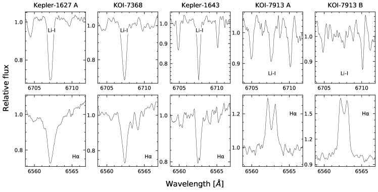
Figure 3: Spectroscopic youth diagnostics for Kepler-1627, KOI-7368, Kepler-1643, and KOI-7913 AB. The spectra are shown in the observed frame, and the stars are sorted left-to-right in order of decreasing effective temperature.

Figure 3 shows key portions of the HIRES and TRES spectra for the Kepler objects in Cep-Her. Lithium absorption is obvious at 6708Å in all stars except KOI-7913 B. H$\alpha$ is in emission for both components of KOI-7913, and in absorption for the hotter stars. Here, we compare these observations against benchmark open clusters in order to assess their implications for the stellar ages.

3.4.1 Lithium

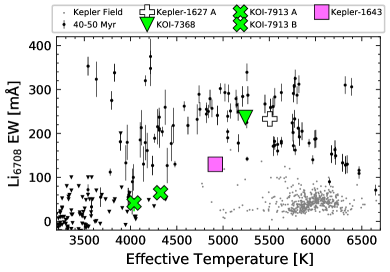
(a)

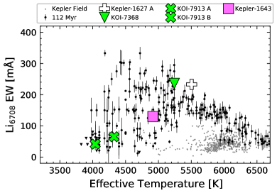
(b)

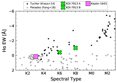
(c)

Figure 4: Lithium 6708Å and H$\alpha$ equivalent widths for the objects of interest compared to young open clusters and field stars. Positive equivalent width means absorption; negative equivalent width means emission. Top & middle: The field stars are KOIs from Berger et al. (2018). The “40-50 Myr” reference stars (left) are from IC 2602 (Randich et al., 2001) and Tuc-Hor (Kraus et al., 2014). The “112 Myr” stars are from the Pleiades (Soderblom et al., 1993; Jones et al., 1996; Bouvier et al., 2018). The statistical uncertainties on the equivalent widths are shown, or else are smaller than the markers. Bottom: The H$\alpha$ comparison is against Tuc-Hor ($\approx$$40$ Myr; Kraus et al., 2014) and the Pleiades (Fang et al., 2018).

Figure 4 compares the measured lithium equivalent widths of the Kepler objects against a few reference populations. We selected reference studies from the literature only when upper limits were explicitly reported. KOI-7368 and KOI-7913 A have secure lithium detections, while for KOI-7913 B the detection is marginal (${\rm EW}_{\rm Li}=42^{+12}_{-19}$ mÅ). For all three stars, as well as for Kepler-1627 A, the observed lithium equivalent width is consistent with the stellar effective temperatures and a $\approx 40$ Myr age.

Kepler-1643, in RSG-5, is conspicuously below the 40-50 Myr sequence in the top panel of Figure 4, though above the field stars (${\rm EW}_{\rm Li}=130^{+6}_{-5}$ mÅ).

Quantitatively, there are 14 reference stars within $\pm$150 K of Kepler-1643. The mean and standard deviation of their lithium EWs is $255\pm 31$ mÅ, which implies that Kepler-1643 is $4.0$-$\sigma$ discrepant from expectations.

The middle panel shows a comparison against the Pleiades, where Kepler-1643 is more consistent with the observed dispersion in lithium.

One explanation for the low Li equivalent width in Kepler-1643 relative to the comparison stars could be that it is a field interloper; another could be that RSG-5 is much older than 50 Myr. We do not favor either explanation. RSG-5 cannot be much older than 50 Myr based on its proximity to the $\delta$ Lyr cluster and IC 2602 in the CAMD, and because it is below the Pleiades in the rotation versus color diagram (Figure 2). Kepler-1643 also seems highly unlikely to be a field interloper, because we demonstrated a few-percent false positive probability in our spatio-kinematic selection of RSG-5 members, and there is a similar independent chance ($\approx$$1\%$) of a field K2V star having a rotation period below the Pleiades (McQuillan et al., 2014). This yields a puzzle: how could a star have spatial, kinematic, and rotational evidence consistent with being in a $\approx$50 Myr cluster, but a low lithium content?

Our preferred explanation for Kepler-1643’s meager lithium content is that the reference samples of IC 2602 and Tuc-Hor stars may not fully explore all possible lithium equivalent widths at this age. This would be somewhat surprising since over a dozen stars have already been analyzed in the relevant effective temperature range. However, considering the top panels of Figure 4, it is also remarkable that in 50 million years, stars between $4500$ K and $5200$ K go from having a tight lithium sequence to one with a dispersion $\approx$$10\times$ greater. The existence of the Li dispersion in Pleiades-age K-dwarfs has been known for decades; it has also been known that the stars with the largest lithium abundances are also the most rapidly rotating (Butler et al., 1987; Soderblom et al., 1993). More recent analyses of this correlation have been reviewed by Bouvier (2020). The conclusion of that work was that the origin of the rotation-lithium correlation likely lies within pre-main-sequence stellar physics. If so, one would expect the IC 2602 and Tuc-Hor K-dwarfs to show a larger intrinsic lithium dispersion. A recent analysis of the $\approx$40 Myr NGC 2547 by Binks et al. (2022) suggests that this may be the case, though that study only had $\approx$10 stars in the relevant effective temperature range. An alternative explanation could be that the overall metallicity of Cep-Her is different from Tuc-Hor and IC 2602, but this seems unlikely given the near-solar metallicities we have measured for the Kepler Objects of Interest. Broadly, these considerations suggest that Cep-Her is a worthy object for further spectroscopic analyses of lithium near the zero-age main sequence.

3.4.2 H$\alpha$

As shown in Figure 3, H$\alpha$ is in emission for both components of KOI-7913, and in absorption for the hotter stars. Additionally, the emission appears double-peaked for both of the KOI-7913 components. An important note is that KOI-7913 A and KOI-7913 B were spatially resolved from each other during data acquisition. Performing a cross-correlation between each of the stars and the nearest matches in the Keck/HIRES template library, we also found that the CCFs for both components of KOI-7913 showed no indications of double-lined binarity (Kolbl et al., 2015).

Balmer line emission, particularly in H$\alpha$, is expected for low-mass stars of this age. Kraus et al. (2014) for instance, in their survey of Tuc-Hor ($\approx$40 Myr), observed that all cluster members with spectral types $>$${\rm K4.5V}$ had H$\alpha$ in emission. This is consistent with our observations: KOI-7913 shows H$\alpha$ in emission for both components, and in absorption for all of our other Kepler objects (Figure 3, lower panel). The double-peaked nature of the emission, though not always present, is also common for active stars. Proxima Centauri, for instance, has double-peaked H$\alpha$ emission (Collins et al., 2017). Given that we have ruled out spectroscopic binarity, the most likely explanation is self-absorption: photons near the center of the line see a greater optical depth from higher layers of the chromosphere, while photons on the wings are too far from the rest wavelength to excite electrons and be re-absorbed in the upper layers. The exact details of when a star’s atmosphere reaches the conditions for such self-absorption require non-local thermal equilibrium models of the chromosphere (Short & Doyle, 1998; Fuhrmeister et al., 2005).

4 The Planets

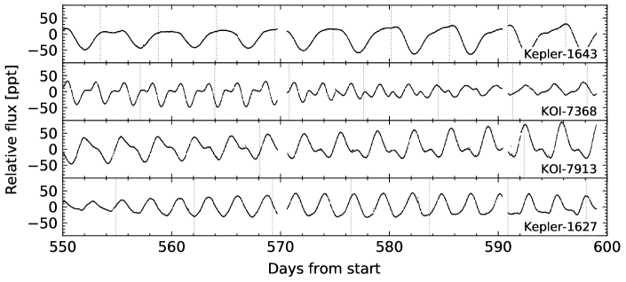
(a)

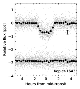
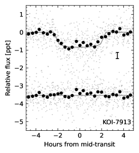
(b)

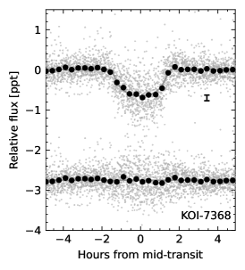
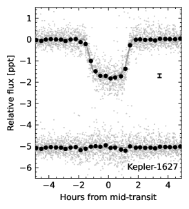
(c)

Figure 5: Raw and processed light curves for the Kepler Objects of Interest in Cep-Her. Top: 50 day light curve segment from the 3.9 years of Kepler data. The ordinate shows the PDCSAP median-subtracted flux in units of parts-per-thousand ($\times 10^{-3}$). The dominant signal is from starspots; planetary transit times are indicated with vertical dashed lines, but the individual transits are not visible at this scale. Bottom: Phase-folded transits of Kepler-1643, KOI-7913, KOI-7368, and Kepler-1627 with stellar variability removed. The maximum a posteriori model is shown with the gray line, and the residual after subtracting the transit model is vertically displaced. Windows over 10 hours are shown. Gray points are individual flux measurements; black points are binned to 20 minute intervals, and have a representative 1-$\sigma$ error bar in the center-right of each panel.

4.1 Kepler Data

The Kepler space telescope observed Kepler-1643, KOI-7913, and KOI-7368 at a 30-minute cadence between May 2009 and April 2013. For all three systems quarters 1 through 17 were observed with minimal data gaps. The top panel of Figure 5 shows a 50-day slice of the PDCSAP light curves for the three new Cep-Her candidates, along with Kepler-1627. In PDCSAP, non-astrophysical variability is removed through a cotrending approach that uses a set of basis vectors derived by applying singular value decomposition to a set of systematics-dominated light curves (Smith et al., 2017). In our analysis, we used the PDCSAP light curves with the default optimal aperture (Smith et al., 2016). Cadences with non-zero quality flags were omitted. In all cases, the stars are dominated by spot-induced modulation with peak-to-peak variability between 2% and 10%. These signals are much larger than the transits, which have depth $\approx$0.1%. To quantify the stellar rotation periods, we calculated the Lomb-Scargle periodogram for each Kepler quarter independently. The resulting means and standard deviations are in Table 1.

4.2 Transit and Stellar Variability Model

Our goals in fitting the Kepler light curves are twofold. First, we want to derive accurate planetary sizes and orbital properties. Second, we want to remove the spot-induced variability signal to enable a statistical assessment of the probability that the transit signals are planetary.

We fitted the data as follows. Given the transit ephemeris from Thompson et al. (2018), we first trimmed the light curve to a local window around each transit that spanned three transit durations before and after each transit midpoint. The out-of-transit points in each local window were then fitted with a fourth-order polynomial, which was divided out from the light curve. The resulting flattened transits were then fitted with a transit model that assumed quadratic limb darkening. The model therefore included 8 free parameters for the transit ($\{P,t_{0},\log R_{\rm p}/R_{\star},b,u_{1},u_{2},R_{\star},\log g\}$), 2 free parameters for the light curve normalization and a white noise jitter ($\{\langle f\rangle,\sigma_{f}\}$), and 5 fixed parameters for each transit.

We fitted the data using exoplanet (Foreman-Mackey et al., 2020). We assumed a Gaussian likelihood, and sampled using PyMC3’s No-U-Turn Sampler (Hoffman & Gelman, 2014), after having initialized to the the maximum a posteriori (MAP) model. We used the Gelman & Rubin (1992) statistic, $\hat{R}$, as our convergence diagnostic. The resulting fits are shown in the lower panels of Figure 5, and the important derived parameters are in Table 1. The set of full parameters and their priors are given in Appendix B.

A potential drawback of our approach is that to remove the starspot-induced variability, we fixed 5 parameters per transit to their MAP values. An alternative could be to fit the planetary transits simultaneously with the starspot-induced variability using a quasiperiodic Gaussian process (GP). We explored this approach, but ultimately prefer our model for its simplicity, and for the benefit that the white noise jitter never trades off with any parameter equivalent to a damping timescale for the coherence of the GP. It is also computationally efficient, and it captures the planetary parameters about which we care the most.

4.3 Planet Validation

In the future, it may be possible to obtain independent evidence for the planetary nature of the Cep-Her planets, for instance by observing spectroscopic transits. For now, it is of interest whether the transit signals might be astrophysical false positives, or whether they are statistically more likely to be planetary. We adopt the Bayesian framework implemented in VESPA to assess the relevant probabilities (Morton, 2012, 2015). Briefly summarized, the priors in VESPA assume the binary star occurrence rate from Raghavan et al. (2010), direction-specific star counts from Girardi et al. (2005), and planet occurrence rates as described by Morton (2012, Section 3.4). The likelihoods are then evaluated by forward-modeling a synthetic population of eclipsing bodies for each astrophysical model class, in which each population member has a known trapezoidal eclipse depth, total duration, and ingress duration. These summary statistics are then compared against the actual photometric data to evaluate the probabilities of false positive scenarios such as foreground eclipsing binaries, hierarchical eclipsing binaries, and background eclipsing binaries.

Kepler-1643

Kepler-1643 b (KOI-6186.01) was already validated as a transiting planet by Morton et al. (2016), who found a probability for any of the aforementioned false positive scenarios of 9$\times$10^-6. Repeating the calculation with our own stellar-variability correction and the new NIRC2 imaging constraints, we find ${\rm FPP}=6\times 10^{-9}$. Figure 5 shows the justification: the transit is flat and has a high S/N ($\approx$$47$). The shape is therefore nearly impossible to reproduce with eclipsing binary models.

Intriguingly, Kepler-1643 failed one of the data validation centroid shift tests (see the q1_q17_dr25_koi data release): the angular distance between the target star’s KIC catalog position and the position of the transiting source was measured as $1\farcs 0$ at 4.4-$\sigma$. The reports show however that two outlying quarters (2 and 6) drive the offset — the centroid locations from the other Kepler quarters are consistent at $\lesssim 0\farcs 4$ (3-$\sigma$). Bryson et al. (2013) showed that for typical field star KOIs without centroid offsets, the mean offset distribution peaks at 0.3^′′ (their Figure 23). By comparison, stars with centroid offsets that can be localized to nearby stars have a distribution that peaks at 7^′′ (their Figure 32). The stellar variability in Kepler-1643 complicates the centroid-based vetting tests, because the shifts measured by these tests are determined from the in- and out-of-transit flux-weighted centroids. For stars with significant spot-induced variability there is no static baseline in either the in- or out-of-transit phases, and so the centroid location may shift depending on the rotation phase combined with the local scene. Based on these considerations, the centroid-level diagnostics for Kepler-1643 appear to be consistent with the transit signal being localized to the target star.

KOI-7368

KOI-7368.01 is listed on the NASA Exoplanet Archive as a “candidate” planet. Morton et al. (2016) did not compute a false positive probability for the system because their default trapezoidal fitting routine failed, presumably due to the spot-induced variability. Our fitting approach rectifies this point, and our new NIRC2 images revealed no new stellar companions. Performing the relevant calculation, we find ${\rm FPP}=4\times 10^{-3}$. Though not as convincing as Kepler-1643, this clears the threshold probability of 1 in 100 suggested by Morton et al. (2016) for calling a planet statistically validated. The S/N of the transit is $\approx$$32$, which indicates that it is unlikely to be caused by systematic noise in the light curve (see Figure 5). The positional probability calculated by Bryson & Morton (2017) also indicates that the transit signal shares its position with the target star.

It bears mentioning that KOI-7368 shows a centroid shift in the q1_q17_dr25_koi validation reports, similar to Kepler-1643. For KOI-7368, the reported offset is smaller, and less formally significant ($0\farcs 2$; 3.0-$\sigma$). Again, the data validation reports show that the shift is caused by a few outlying quarters (4, 5, 8, and 12). Since the remaining quarters show consistent scatter in their centroid locations, these outlying quarters are likely also caused by the stellar variability, because their directions are inconsistent across different quarters. Our NIRC2 imaging independently shows that there are no known neighboring sources that could cause an offset of the observed amplitude, as is also the case for Kepler-1643.

KOI-7913

KOI-7913.01 is also currently listed on the NASA Exoplanet Archive as a “candidate” planet. The Morton et al. (2016) analysis was of Q1-Q17 KOIs from DR24, and therefore spanned KOI-1.01 to KOI-7620.01 (omitting KOI-7913.01). However the results of the subsequent DR25 analysis by Morton et al. are listed at the NASA Exoplanet Archive. The relevant table gives a probability for the system being an astrophysical false positive of $1.4\times 10^{-4}$, with the most likely false positive scenario being a blended eclipsing binary. Repeating the calculation with our new detrending and NIRC2 contrast curves, we find a similar result: ${\rm FPP}=1.3\times 10^{-4}$. Though the transit has the lowest S/N of any of the objects discussed ($\approx$$14$), its low FPP can be understood through its flat-bottomed shape, combined with its long transit duration relative to most eclipsing binary models (Figure 5). The positional probability calculation performed by Bryson & Morton (2017) yielded a near-unity probability that the transit event is at the same location as the host star, and so the cumulative evidence suggests that KOI-7913 Ab is indeed a statistically validated planet. Its disposition has however previously fluctuated from “false positive” to “candidate” (see Appendix C). The most likely explanation is the presence of KOI-7913 B, which is located $\approx 0.9$ Kepler pixels away from Kepler-7913 A. While the $\approx$1.5 pixel FWHM of the Kepler pixel response function implies that there is blending between the two stars, the target-pixel level data for KOI-7913 B reveals an entirely different stellar rotation period (Table 1), and no hint of the transit signal. This implies that KOI-7913 B cannot host the planet.

5 Discussion & Conclusion

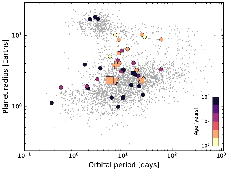
Figure 6: Radii, orbital periods, and ages of transiting exoplanets. Planets younger than a gigayear with ages more precise than a factor of three are emphasized. The Cep-Her planets are Kepler-1643 b ($\square$), KOI-7368 b ($\triangledown$), KOI-7913 Ab (X), and Kepler-1627 Ab (+). Interesting trends in the population of planets younger than $10^{8}$ years old include i) their large sizes and ii) the lack of hot Jupiters. The new objects of interest in Cep-Her have normal mini-Neptune sizes between 2 and 3 $R_{\oplus}$, which is a novelty given their ages. Parameters are from the NASA Exoplanet Archive (2022).

5.1 Normal-Sized Mini-Neptunes Exist at 40 Myr

The most significant novelty about the planets in Kepler-1643, KOI-7368, and KOI-7913 is that their sizes (2.2 to 2.3 $R_{\oplus}$) are normal relative to the known population of mini-Neptunes from Kepler. At field star ages, mini-Neptune sizes span 1.8 $R_{\oplus}$ to 3.6 $R_{\oplus}$, with the most common size being $\approx 2.4\,R_{\oplus}$ (Fulton et al., 2017). The known planets younger than $10^{8}$ years are almost all larger, with sizes between 4 and 10$\,R_{\oplus}$ (Mann et al., 2016; David et al., 2016; Benatti et al., 2019; David et al., 2019; Newton et al., 2019; Rizzuto et al., 2020; Bouma et al., 2020; Mann et al., 2022). Figure 6 explores this by showing the sizes, orbital periods, and ages of the known transiting planets, emphasizing planets with precise ages. The smallest previously known planets comparable to the new Cep-Her mini-Neptunes are AU Mic c ($3.0\pm 0.2\,R_{\oplus}$, see Martioli et al. 2021 and Gilbert et al. 2022), Kepler-1627 Ab ($3.8\pm 0.2\,R_{\oplus}$; Bouma et al. 2022), and AU Mic d ($4.2\pm 0.2\,R_{\oplus}$; Plavchan et al. 2020).

The theoretical expectation is that mini-Neptunes with sizes of 2 to 3 $R_{\oplus}$ should be common at ages of $10^{7}$ to $10^{8}$ years. This expectation is tied to inferences about the initial distributions of planetary core mass, core composition, and atmospheric mass fraction (Owen & Wu, 2017). The Kelvin-Helmholtz cooling timescale, which is tied to the entropy of the planetary interior shortly after disk dispersal, also plays a significant role (Owen, 2020). As an example, Rogers & Owen (2021) predicted that given a core mass distribution peaked at $\approx$$4$ $M_{\oplus}$, an ice-poor rock/iron core composition, and a typical H/He mass fraction of $\approx$4%, there should be a single local maximum in planet occurrence rates at 2 to 3 $R_{\oplus}$, at times between 10 and 100 Myr. In other words, Rogers & Owen (2021) predict the existence of a “radius mountain” at these early times, rather than a “radius valley”. The models advanced by Gupta & Schlichting (2020) and Lee & Connors (2021) agree that this local maximum should exist; their differences lie in the mechanism for producing the radius valley, and in whether a population of rocky planets is predicted to exist at the time of disk dispersal.

Systems such as K2-25, V1298 Tau, HIP-67522, TOI-837, and TOI-1227 have sizes that are anomalously large relative to the predicted peak in planet occurrence at 2 to 3 $R_{\oplus}$. However, their large sizes can be accommodated by invoking any of i) larger core masses, ii) more volatile-rich compositions, iii) larger initial atmospheric mass fractions, or iv) longer thermal cooling times. Secure mass measurements would help constrain this parameter space, but the $\sim$1  km s^-1 spot-induced radial velocity semi-amplitudes make measuring the Doppler orbits very difficult (Cale et al., 2021; Zicher et al., 2022; Klein et al., 2022). Regardless, the new Kepler-1643, KOI-7368, and KOI-7913 systems do demonstrate that at least some planets at 40 Myr have sizes that are consistent with theoretical expectations for mini-Neptunes. While selection effects imposed by spot-induced photometric variability are a likely explanation for why planets this small have not previously been identified (e.g., Zhou et al., 2021), future work should quantify this bias more carefully, in order to enable empirical studies of how the planetary size distribution changes at early times.

5.2 Is CH-2 a Coeval Population?

RSG-5, and Kepler-1643’s membership inside it, meet typical expectations for a star claimed to be in an open cluster. RSG-5 is an obvious overdensity relative to the local field, and our membership selection easily yielded a clean pre-main-sequence locus (Figure 2). CH-2, and KOI-7913 and KOI-7368’s membership inside it, do not meet these expectations in as obvious a manner. This is because the CH-2 association is diffuse.

To quantify the density difference between CH-2 and RSG-5, we can compare the spatial and velocity volumes searched for each group. For RSG-5, we drew 173 candidate members from a $30\,{\rm pc}\times 30\,{\rm pc}\times 40\,{\rm pc}$ rectangular prism, given a $1.5{\rm{\rm\,km\,s^{-1}}}\times 2.5{\rm{\rm\,km\,s^{-1}}}$ rectangle in apparent galactic velocity. For CH-2, our 37 candidate members came from a rectangular prism of dimension $50\,{\rm pc}\times 40\,{\rm pc}\times 30\,{\rm pc}$, and a rectangular box of $2{\rm{\rm\,km\,s^{-1}}}\times 4{\rm{\rm\,km\,s^{-1}}}$. If we define the searched volume in units of ${\rm pc}^{3}\,{\rm km^{2}}\,{\rm s^{-2}}$, then the volume ratio of CH-2 to RSG-5 is 3.5 to 1. The ratio of number densities (candidate members per unit searched volume) in RSG-5 relative to CH-2 is 16 to 1.

Given its low density, is CH-2 truly a star cluster? For this discussion, we adopt the definition that a star cluster is a group of at least 12 stars that was physically associated at its time of formation. The “12” is set to distinguish star clusters from high-order multiples (see Krumholz et al., 2019). We explicitly do not require a “star cluster” to be gravitationally bound: dissolved clusters as well as their tidal tails are included in our adopted definition of “clusters”. We similarly do not require a threshold number of stars per unit spatial volume. The latter point acknowledges that an important factor in cluster identification is also coherence in velocity space. For instance, the Psc-Eri stream, which has a shape that can be approximated as a 600 parsec-long cylinder with a radius of 30 parsecs, has a number density roughly a factor of three times lower than even CH-2 (Röser & Schilbach, 2020). However its existence is discernible because of the $\lesssim 2.5$ km s^-1 scatter in its cylindrical velocities. Perhaps once stellar rotation periods and chemical abundances reach the same level of ubiquity as stellar proper motions, they might enable further refinement in our ability to discover stars that formed as part of the same event.

From a data-driven perspective, demonstrating that a group of stars was physically associated at its time of formation is challenging. While some young groups show kinematic evidence for expansion (Kuhn et al., 2019), many, including Sco-Cen, do not (Wright & Mamajek, 2018). This complicates the feasibility of deriving kinematic ages through traceback, as well as through the expansion itself (see Crundall et al., 2019). A more minimal approach is that suggested by Tofflemire et al. (2021): search for coeval, phase-space neighbors, measure their ages, and determine if they share a common age. This approach can demonstrate whether a star is currently associated with a set of coeval stars, though it falls short of determining what the association looked like in the past. Our analysis of CH-2 meets the latter standard for demonstrating the existence of a $\approx$40 Myr stellar association.

It would be a worthy exercise to perform a similar search for coeval phase-space neighbors on the entire dataset of known exoplanet hosts. For the time being, we can offer the anecdotal point that in our experience, most stars do not have dozens of 40 Myr neighbors within a local volume of a few ​ km s^-1 and tens of parsecs.

5.3 Future work

Cep-Her

Our analysis to date has focused only on portions of Cep-Her that were observed by Kepler: RSG-5, CH-2, and the $\delta$ Lyr cluster. In Bouma et al. (2022) as well as this work, we have shown that these groups share similar ages, and have kinematic correlations that suggest a common origin. With that said, the membership and kinematics of the other Cep-Her groups shown in Figure 1 deserve independent attention. An important aspect of the remaining work will be to acquire radial velocities for a larger subset of the stars, and to determine whether the traceback approach could be applicable. Wide-field spectroscopic surveys such as LAMOST (Zhao et al., 2012) or SDSS-V (Kollmeier et al., 2017) could enable such analyses for the brightest members, while also providing sensitivity to the Li 6708 Å line. The Gaia DR3 RVS spectra (released during review of this manuscript) could contain similar velocity information down to spectral types of $\approx$K5V ($G_{\rm RVS}\lesssim 14$), and perhaps also enable analyses of the calcium infrared triplet as a youth indicator. The combination of more complete kinematics and youth indicators would help in definitively unraveling the formation history of the complex.

A number of worthy photometric projects also seem possible given the new understanding of Cep-Her. One is asteroseismology of the $\delta$ Sct stars, using either TESS or Kepler data (Bedding et al., 2020). For cases in which the modes are resolved, this might yield age or metallicity estimates for the subgroups independent of other methods. Other projects could include a more comprehensive analysis of the stellar rotation periods, searches of the Kepler light curves for exocomets (Zieba et al., 2019), and searches for missed planets around the most rapid rotators.

Exoplanet demographics at early times

Our main motivation for finding new young planets is to help benchmark models for planetary evolution. However demographic analyses of the known planets between $10^{7}$ and $10^{9}$ years have so far been rather limited. Approximately 40 such planets are now known (Figure 2). About half come from K2, a quarter from TESS, and now a quarter from Kepler.

Given the current state of the field, a few reflections regarding experimental design of a demographic survey focused on planetary evolution over the first gigayear might be useful. The first is that such a project requires a set of target stars with known ages. A promising way to compile relevant stars could be to combine automated spatio-kinematic clustering from Gaia with rotation periods measured using TESS (see the appendices of Bouma et al., 2022). The second consideration is that all the known young planets smaller than $3$ $R_{\oplus}$ come from either K2 or Kepler. Demographic inferences based on TESS are therefore limited to planetary sizes $\gtrsim 4$ $R_{\oplus}$, for planets close-in to their host stars. It would be worthwhile to compare the occurrence rates of both types of planets with those from the main Kepler sample. One specific question that seems within reach would be to clarify whether enough young stars have been searched for the dearth of young hot Jupiters to be significant. Since the hot Jupiter occurrence rate is strongly dependent on stellar mass and metallicity (Petigura et al., 2018, 2022), particular care would be needed to select a sample of well-studied FGK dwarfs for the measurement, likely using stars in Sco OB2, Cep-Her, and Orion. For demographic studies focused on how mini-Neptune sizes evolve, the combined K2 and Kepler dataset would be the better primary source.

5.4 Summary

We have shown that Kepler-1643 b, KOI-7368 b, and KOI-7913 Ab are 40 to 50 million years old, and that each system is most likely planetary. The evidence for the planetary interpretation comes from an application of VESPA to the Kepler data, alongside new imaging from NIRC2. The validity of the VESPA framework rests on the premise that non-astrophysical false positives can be rejected. This seems to be the case for all three objects, even though Kepler-1643 and KOI-7368 both show weak centroid offsets in specific quarters. For both systems, the observed shifts are consistent with being caused by starspot-induced variability in specific quarters spuriously moving the stellar center-of-light. Independently, our imaging rules out companion stars with the brightnesses and positions that would be needed to explain the reported shifts. All three objects are therefore most likely planets.

Each system has multiple indicators of youth that support the reported ages. For Kepler-1643, the strongest youth indicator is its physical and kinematic association with RSG-5. Based on the color–absolute magnitude diagram, we are able to select members of this cluster with a false positive rate of a few percent (Figure 2). Kepler-1643 is one such member. While the stellar rotation period period agrees with this assessment, the star’s lithium equivalent width is marginally low, which might motivate future exploration of lithium depletion across FGKM stars in RSG-5 (see Section 3.4).

The spatio-kinematic argument for the youth of KOI-7368 and KOI-7913 is weaker because they are in an association of stars, CH-2, that is more diffuse. For KOI-7913, stronger indicators of its age come from its binarity. Both stellar components in KOI-7913 have isochronal ages consistent with $40$ Myr. Both components also show H$\alpha$ in emission, which for the transit-hosting $\approx$K6V primary is a strong indicator that the star is $\lesssim$100 Myr old. KOI-7368 is more massive, and its Li 6708 Å measurement and stellar rotation period provide independent verification of the star’s youth.

The astrophysical implication of these considerations is that planets $\approx$2 Earth radii in size exist at ages of 40 million years. It will be interesting to continue the push down to smaller planetary sizes at comparable ages – the planetary detections we have presented are well above the average detection significance for Kepler planets. There may still be room at the bottom.

Appendix A Candidate Cep-Her Members

Table 2

contains 338 candidate Cep-Her members with weights $D>0.02$ observed by Kepler. The complete catalog of candidate Cep-Her members will be provided by R. Kerr et al. in prep. using Gaia DR3; Table 2 is from an early version of that analysis based on Gaia EDR3. Note that more restrictive weight cuts should be imposed if one wishes to remove the majority of field star interlopers. Table 2 was created by cross-matching candidate Cep-Her members (selected using Gaia EDR3; Section 2.2) against a Kepler to Gaia DR2 cross-match (the gaia-kepler.fun crossmatch database created by Megan Bedell). The kic_dr2_ang_dist column is from the latter table. The EDR3 to DR2 match was performed using the gaiaedr3.dr2_neighbourhood table, and the closest proper motion and epoch-corrected angular distance neighbor was taken as the single best match. The edr3_dr2_mag_diff column gives some indication of the reliability of this EDR3 to DR2 conversion, as there are a few cases between Gaia DR2 and EDR3 where partially resolved binaries became fully resolved.

Candidate matches between Cep-Her and the Kepler Objects of Interest:

The full list of candidate matches between Cep-Her and the Kepler Objects of Interest is as follows – the objects are listed in order of descending weights, $D$. Objects designated as confirmed planets included Kepler-1627, Kepler-1643, Kepler-1331, Kepler-1062, and Kepler-1933. Objects designated as candidate planets included KOI-5264, KOI-8007, KOI-7572, KOI-7375, KOI-7368, KOI-7638, KOI-5632, and KOI-7913. Objects designated known false positive planet candidates included KOI-6437, KOI-5988, KOI-7871, KOI-7655, KOI-5024, KOI-61, KOI-4336, KOI-6812, KOI-3399, and KOI-6277. Finally, Kepler-1902 (KOI-3090) has one confirmed planet (KOI-3090.02), and one false positive (KOI-3090.01). Of these objects, only Kepler-1627, Kepler-1643, KOI-7368, and KOI-7913 met our requirements for potentially both i) having real planets, and ii) being $\lesssim 10^{8}$ years old, based on the presence of rotational modulation at the expected period and amplitude. Of the 14 confirmed and candidate planets, 6 failed the first filter, and 7 independently failed the second. One object was ambiguous: Kepler-1933. This system has a confirmed $\approx$$1.4\,R_{\oplus}$ planet, a stellar rotation period of 6.5 days, and an effective temperature of $\approx$$5750\,{\rm K}$. This places it near the upper envelope of the rotation period vs. color distribution for the Pleiades, making it unlikely to be $\approx$40 Myr old. Nonetheless, we acquired a reconnaissance HIRES spectrum, and it yielded ${\rm EW}_{\rm Li}=93\pm 5$ mÅ. Combined with the rotation period, this suggests an age for Kepler-1933 between 100 and 300 Myr. Based on these indicators, the system is unlikely to be part of Cep-Her, but could merit further study.

Table 3

contains spatial, kinematic, astrometric, and rotation period information for the 173 candidate RSG-5 members and 37 candidate CH-2 members described in Section 2.2. These are the data used to make the lower panels of Figure 2; as with Table 2, these are from a preliminary version of the SPYGLASS 1 kpc expansion (R. Kerr et al. in prep). We adopted the ZTF period over the TESS period in three cases: (1) Gaia EDR3 2081755809272821248: the top ZTF Lomb-Scargle peak gave 6.61 days, while our default pipeline favored a TESS peak of 13.34 days; manual inspection of the light curve favors the former; (2) Gaia EDR3 2081737529891330560: we found 3.06 days with TESS and 6.64 days with ZTF; we suspect that TESS captured the 1/2-period harmonic and adopt the approximately double value from ZTF; (3) 2134851775526125696: for this star, we measured 1.91 days with TESS from Cycle 2, but noted that the signal appeared to be missing in Cycle 4; ZTF found a strong signal at 12.23 days and we adopt this as the star’s period. In the remaining overlap cases, we adopted the average between TESS and ZTF as the final period. For these overlap stars, the median absolute deviation is 0.01 days, showing remarkable consistency between the surveys. For three stars, we failed to detect a period in TESS but recovered one from ZTF; in all cases the periods appear to be 13–16 days. These stars were: (1) Gaia EDR3 2129930258400157440, for which TESS showed a flat light curve while ZTF yielded a 15.3-day period; (2) Gaia EDR3 2082376861542398336, LS found a 7.6-day period which we rejected during visual validation; we found 15.4 days with ZTF, and we suspect that the weak/rejected signal form TESS might have been a 1/2 period harmonic; (3) Gaia EDR3 2082397099429013120, similar to the previous case, we rejected a 6.7-day signal from TESS and recovered a 12.8-day period with ZTF.

Appendix B Table of Transit Fit Parameters

Table 4 gives the full set of fitted and derived parameters from the model described in Section 4.2. Priors and convergence statistics are also listed.

Appendix C Disposition History of KOI-7913

The disposition of KOI-7913.01 has been debated: in q1_q17_dr25_koi the source was flagged as a false positive, with the comment “cent_kic_pos—halo_ghost”. This comment and disposition were removed in the q1_q17_dr25_sup_koi data release, which renamed the planet a “candidate”. In this note, we discuss the interpretation of these flags (which do not apply to the system, according to the latest analysis). We also discuss how the relative on-sky positions of KOI-7913 A and KOI-7913 B affect the interpretation of the Kepler data.

As described by Thompson et al. (2018), the “cent_kic_pos” flag is an indication that the measured source centroid is offset from its expected location in the Kepler Input Catalog. The final Kepler data validation reports, generated 2016 Jan 30, do not show this to be the case for KOI-7913. Moreover, the statistical significance of any centroid offset is lower than for KOI-7368 and Kepler-1643 (which both show centroid offsets that are likely explained by the stellar variability).

What of the “halo_ghost” flag? This test measures the transit strength for the pixels inside the aperture, and compares it to that measured in the ring of pixels around said aperture (the “halo”). One usually expects the transit signal to be strongest in the central aperture, rather than the halo. Two types of false positive scenarios can change this and trigger the flag: the first is when optical ghosts from bright eclipsing binaries reflect off the CCD, and contaminate the target star. The second is when the PRF of nearby stars directly overlaps with the PRF of the target star (see Thompson et al. 2018, Section A.5.2). The most obvious explanation for KOI-7913 is the latter case, given that KOI-7913 B is $\approx 0.9$ Kepler pixels away from Kepler-7913 A and so it usually part of the “halo”. Due to the on-sky orientation of KOI-7913 A and KOI-7913 B, the default “optimal aperture” selected in quarters 3, 7, 11, and 15 in fact included both stars, while for the remaining quarters KOI-7913 B was excluded from the optimal aperture but was included as part of the halo (see pages 35 through 71 of the data validation reports.)

Given the orientation of the stars and the $\approx$1.5 pixel FWHM of the Kepler pixel response function, some blending between the two stars is present. The pointing geometries from quarters 3, 7, 11, and 15 however did not affect the observed transit depths, which is an indication that the crowding metric applied in the data products accurately correct the mean flux level (Morris et al., 2017). Analysis of the target-pixel data that was separately acquired for KOI-7913 B also reveals a different stellar rotation period, and no hint of the transit signal.

Table 2: Candidate Cep-Her members observed by Kepler

Parameter	Example Value	Description
dr2_source_id	2073765172933035008	Gaia DR2 source identifier.
dr3_source_id	2073765172933035008	Gaia (E)DR3 source identifier.
kepid	5641711	KIC identifier.
ra	297.40986	Gaia EDR3 right ascension [deg].
dec	40.89719	Gaia EDR3 declination [deg].
weight	0.041	Strength of connectivity to other candidate cluster members.
v_l	-0.51	Longitudinal galactic velocity, $v_{l^{*}}$ [km s-1].
v_b	-8.23	Latitudinal galactic velocity [km s-1].
x_pc	-8035.4	Galactocentric $X$ position coordinate [pc].
y_pc	331.4	Galactocentric $Y$ position coordinate [pc].
z_pc	65.3	Galactocentric $Z$ position coordinate [pc].
kic_dr2_ang_dist	0.298	Separation between KIC and Gaia DR2 positions [arcsec].
edr3_dr2_mag_diff	0.002	$G$-band difference between EDR3 and DR2 source match [mag].

Note. — Table 2 is published in its entirety in a machine-readable format. One entry is shown for guidance regarding form and content.

Table 3: Rotation periods and kinematics for candidate RSG-5 and CH-2 members.

Parameter	Example Value	Description
dr3_source_id	2127562009133684480	Gaia (E)DR3 source identifier.
ra	291.02306	Gaia EDR3 right ascension [deg].
dec	46.43843	Gaia EDR3 declination [deg].
parallax	3.7099	Gaia EDR3 parallax [milliarcsec].
ruwe	0.981	Gaia EDR3 renormalized unit weight error.
weight	0.087	Strength of connectivity to other candidate cluster members.
v_l	2.78	Longitudinal galactic velocity, $v_{l^{*}}$ [km s-1].
v_b	-2.87	Latitudinal galactic velocity [km s-1].
x_pc	-8068.5	Galactocentric $X$ position coordinate [pc].
y_pc	256.0	Galactocentric $Y$ position coordinate [pc].
z_pc	86.3	Galactocentric $Z$ position coordinate [pc].
(BP-RP)0	-0.115	Gaia $G_{\mathrm{BP}}$-$G_{\mathrm{RP}}$ color, minus $E$($G_{\mathrm{BP}}$-$G_{\mathrm{RP}}$).
(M_G)0	0.442	Absolute $G$-band magnitude, corrected for extinction.
cluster	CH-2	RSG-5 or CH-2.
Prot_Adopted	NaN	Adopted rotation period if available, else NaN [days].
Prot_TESS	NaN	TESS rotation period if available, else NaN [days].
Prot_ZTF	NaN	ZTF rotation period if available, else NaN [days].
Prot_Confused	NaN	Boolean flag; true when stars are photometrically blended.

Note. — Table 3 is published in its entirety in a machine-readable format. One entry is shown for guidance regarding form and content.

Table 4: Priors and posteriors for the transit models with local polynomials removed.

Param.	Unit	Prior	Median	Mean	Std. Dev.	3% HDI	97% HDI	ESS	$\hat{R}-1$
Kepler-1643
$P$	d	$\mathcal{N}(5.34264;0.01000)$	5.3426257	5.3426258	0.0000101	5.3426071	5.3426454	7884	1.1e-03
$t_{0}^{(1)}$	d	$\mathcal{N}(134.38;0.02)$	134.3820	134.3820	0.0011	134.3799	134.3841	7390	3.7e-04
$\log R_{\rm p}/R_{\star}$	–	$\mathcal{U}(-6.215;0.000)$	-3.688	-3.689	0.021	-3.728	-3.653	4449	-7.8e-05
$b$	–	$\mathcal{U}(0;1+R_{\mathrm{p}}/R_{\star})$	0.583	0.578	0.051	0.485	0.673	4705	1.9e-04
$u_{1}$	–	Kipping (2013)	0.26	0.29	0.21	0.00	0.68	5324	7.9e-04
$u_{2}$	–	Kipping (2013)	0.32	0.31	0.32	-0.26	0.88	4908	8.4e-04
$R_{\star}$	$R_{\odot}$	$\mathcal{N}(0.855;0.044)$	0.851	0.851	0.045	0.766	0.933	7473	7.2e-04
$\log g$	cgs	$\mathcal{N}(4.502;0.035)$	4.507	4.507	0.035	4.442	4.576	6530	-1.4e-04
$\log\sigma_{f}$	–	$\mathcal{N}(\log\langle\sigma_{f}\rangle;2.000)$	-8.520	-8.520	0.019	-8.556	-8.486	7966	2.1e-04
$\langle f\rangle$	–	$\mathcal{N}(1.000;0.100)$	1.000	1.000	0.000	1.000	1.000	7488	3.2e-04
$R_{\rm p}/R_{\star}$	–	–	0.025	0.025	0.001	0.024	0.026	4449	-7.8e-05
$\rho_{\star}$	g  cm-3	–	1.94	1.95	0.19	1.60	2.31	6081	9.4e-05
$R_{\rm p}$	$R_{\mathrm{Jup}}$	–	0.207	0.207	0.012	0.184	0.231	6326	2.5e-04
$R_{\rm p}$	$R_{\mathrm{Earth}}$	–	2.32	2.32	0.13	2.06	2.59	6326	2.5e-04
$a/R_{\star}$	–	–	14.31	14.32	0.47	13.49	15.23	6081	8.2e-05
$\cos i$	–	–	0.041	0.040	0.005	0.032	0.049	4929	2.4e-04
$T_{14}$	hr	–	2.41	2.41	0.06	2.30	2.53	4774	5.3e-04
$T_{13}$	hr	–	2.23	2.23	0.07	2.11	2.36	4561	6.2e-04
KOI-7368
$P$	d	$\mathcal{N}(6.84294;0.01000)$	6.8430344	6.8430341	0.0000125	6.8430107	6.8430574	10045	6.5e-05
$t_{0}^{(1)}$	d	$\mathcal{N}(137.06;0.02)$	137.0463	137.0463	0.0014	137.0437	137.0489	10303	9.2e-05
$\log R_{\rm p}/R_{\star}$	–	$\mathcal{U}(-4.605;0.000)$	-3.760	-3.763	0.031	-3.819	-3.708	4043	6.3e-04
$b$	–	$\mathcal{U}(0;1+R_{\mathrm{p}}/R_{\star})$	0.508	0.500	0.064	0.380	0.612	4434	3.5e-04
$u_{1}$	–	Kipping (2013)	0.98	0.95	0.27	0.43	1.42	5809	-5.6e-05
$u_{2}$	–	Kipping (2013)	-0.19	-0.16	0.31	-0.66	0.42	4387	2.6e-04
$R_{\star}$	$R_{\odot}$	$\mathcal{N}(0.876;0.035)$	0.874	0.874	0.036	0.804	0.938	9902	7.3e-04
$\log g$	cgs	$\mathcal{N}(4.499;0.030)$	4.503	4.502	0.030	4.445	4.557	7527	2.7e-05
$\log\sigma_{f}$	–	$\mathcal{N}(\log\langle\sigma_{f}\rangle;2.000)$	-8.314	-8.314	0.012	-8.337	-8.292	10636	1.3e-03
$\langle f\rangle$	–	$\mathcal{N}(1.000;0.100)$	1.000	1.000	0.000	1.000	1.000	9742	-2.9e-04
$R_{\rm p}/R_{\star}$	–	–	0.023	0.023	0.001	0.022	0.025	4043	6.3e-04
$\rho_{\star}$	g  cm-3	–	1.87	1.88	0.15	1.59	2.16	6829	3.4e-04
$R_{\rm p}$	$R_{\mathrm{Jup}}$	–	0.198	0.198	0.011	0.177	0.218	5676	2.8e-04
$R_{\rm p}$	$R_{\mathrm{Earth}}$	–	2.22	2.22	0.12	1.98	2.44	5676	2.8e-04
$a/R_{\star}$	–	–	16.67	16.68	0.45	15.86	17.54	6829	3.3e-04
$\cos i$	–	–	0.030	0.030	0.004	0.022	0.038	4518	5.4e-04
$T_{14}$	hr	–	2.79	2.79	0.07	2.65	2.93	4845	5.0e-04
$T_{13}$	hr	–	2.62	2.62	0.08	2.47	2.78	4575	3.1e-04
KOI-7913
$P$	d	$\mathcal{N}(24.27838;0.01000)$	24.278553	24.278571	0.000263	24.278112	24.279085	4413	1.5e-03
$t_{0}^{(1)}$	d	$\mathcal{N}(154.51;0.05)$	154.5121	154.5124	0.0063	154.4998	154.5237	5612	6.0e-04
$\log R_{\rm p}/R_{\star}$	–	$\mathcal{U}(-5.298;0.000)$	-3.599	-3.602	0.046	-3.689	-3.519	4290	5.6e-04
$b$	–	$\mathcal{U}(0;1+R_{\mathrm{p}}/R_{\star})$	0.312	0.298	0.153	0.005	0.523	2373	1.8e-03
$u_{1}$	–	Kipping (2013)	0.27	0.34	0.28	0.00	0.86	4491	-6.1e-05
$u_{2}$	–	Kipping (2013)	0.21	0.23	0.32	-0.31	0.86	5935	7.0e-04
$R_{\star}$	$R_{\odot}$	$\mathcal{N}(0.790;0.049)$	0.788	0.788	0.049	0.699	0.881	6847	2.8e-04
$\log g$	cgs	$\mathcal{N}(4.523;0.043)$	4.526	4.527	0.042	4.450	4.606	5714	6.6e-04
$\log\sigma_{f}$	–	$\mathcal{N}(\log\langle\sigma_{f}\rangle;2.000)$	-7.197	-7.197	0.019	-7.230	-7.161	6976	1.4e-04
$\langle f\rangle$	–	$\mathcal{N}(1.000;0.100)$	1.000	1.000	0.000	1.000	1.000	6998	2.8e-04
$R_{\rm p}/R_{\star}$	–	–	0.027	0.027	0.001	0.025	0.030	4290	5.6e-04
$\rho_{\star}$	g  cm-3	–	2.20	2.21	0.25	1.78	2.70	5357	5.6e-04
$R_{\rm p}$	$R_{\mathrm{Jup}}$	–	0.209	0.209	0.016	0.179	0.238	4882	1.3e-03
$R_{\rm p}$	$R_{\mathrm{Earth}}$	–	2.34	2.34	0.18	2.01	2.67	4882	1.3e-03
$a/R_{\star}$	–	–	40.92	40.95	1.54	38.14	43.84	5357	6.6e-04
$\cos i$	–	–	0.008	0.007	0.004	0.000	0.013	2344	1.9e-03
$T_{14}$	hr	–	4.39	4.40	0.21	3.98	4.76	3952	5.6e-04
$T_{13}$	hr	–	4.13	4.13	0.22	3.72	4.55	3632	7.6e-04

Note. — ESS refers to the number of effective samples. $\hat{R}$ is the Gelman-Rubin convergence diagnostic. Logarithms in this table are base-$e$. $\mathcal{U}$ denotes a uniform distribution, and $\mathcal{N}$ a normal distribution. (1) The ephemeris is in units of BJKD (BJDTDB-2454833).

References

- Agol et al. (2020) Agol, E., Luger, R., & Foreman-Mackey, D. 2020, AJ, 159, 123
- Akeson et al. (2013) Akeson, R. L., Chen, X., Ciardi, D., et al. 2013, PASP, 125, 989
- Arancibia-Silva et al. (2020) Arancibia-Silva, J., Bouvier, J., Bayo, A., et al. 2020, A&A, 635, L13
- Arevalo et al. (2022) Arevalo, R. T., Tamayo, D., & Cranmer, M. 2022, arXiv:2203.02805 [astro-ph]
- Astropy Collaboration et al. (2018) Astropy Collaboration, Price-Whelan, A. M., Sipőcz, B. M., et al. 2018, AJ, 156, 123
- Bedding et al. (2020) Bedding, T. R., Murphy, S. J., Hey, D. R., et al. 2020, Nature, 581, 147
- Bellm et al. (2019) Bellm, E. C., Kulkarni, S. R., Graham, M. J., et al. 2019, PASP, 131, 018002
- Benatti et al. (2019) Benatti, S., Nardiello, D., Malavolta, L., et al. 2019, A&A, 630, A81
- Berger et al. (2018) Berger, T. A., Howard, A. W., & Boesgaard, A. M. 2018, ApJ, 855, 115
- Bieryla et al. (2021) Bieryla, A., Tronsgaard, R., Buchhave, L. A., et al. 2021, in Posters from the TESS Science Conference II (TSC2), 124
- Binks et al. (2022) Binks, A. S., Jeffries, R. D., Sacco, G. G., et al. 2022, arXiv e-prints, arXiv:2204.05820
- Borucki et al. (2010) Borucki, W. J., Koch, D., Basri, G., et al. 2010, Science, 327, 977
- Bouma et al. (2021) Bouma, L. G., Curtis, J. L., Hartman, J. D., Winn, J. N., & Bakos, G. Á. 2021, AJ, 162, 197
- Bouma et al. (2020) Bouma, L. G., Hartman, J. D., Brahm, R., et al. 2020, AJ, 160, 239
- Bouma et al. (2022) Bouma, L. G., Curtis, J. L., Masuda, K., et al. 2022, AJ, 163, 121
- Bouvier (2020) Bouvier, J. 2020, Mem. Soc. Astron. Italiana, 91, 39
- Bouvier et al. (2018) Bouvier, J., Barrado, D., Moraux, E., et al. 2018, A&A, 613, A63
- Brasseur et al. (2019) Brasseur, C. E., Phillip, C., Fleming, S. W., Mullally, S. E., & White, R. L. 2019, Astrophysics Source Code Library, ascl:1905.007
- Bressan et al. (2012) Bressan, A., Marigo, P., Girardi, L., et al. 2012, MNRAS, 427, 127
- Bryson & Morton (2017) Bryson, S. T., & Morton, Timothy, D. 2017, Kepler Science Document KSCI-19108-001
- Bryson et al. (2013) Bryson, S. T., Jenkins, J. M., Gilliland, R. L., et al. 2013, PASP, 125, 889
- Buchhave et al. (2012) Buchhave, L. A., Latham, D., Johansen, A., et al. 2012, Nature, 486, 375
- Butler et al. (1987) Butler, R. P., Cohen, R. D., Duncan, D. K., & Marcy, G. W. 1987, ApJ, 319, L19
- Cale et al. (2021) Cale, B. L., Reefe, M., Plavchan, P., et al. 2021, AJ, 162, 295
- Campello et al. (2015) Campello, R. J. G. B., Moulavi, D., Zimek, A., & Sander, J. 2015, ACM Transactions on Knowledge Discovery from Data, 10, 5:1
- Cantat-Gaudin et al. (2018) Cantat-Gaudin, T., Jordi, C., Vallenari, A., et al. 2018, A&A, 618, A93
- Choi et al. (2016) Choi, J., Dotter, A., Conroy, C., et al. 2016, ApJ, 823, 102
- Chubak et al. (2012) Chubak, C., Marcy, G., Fischer, D. A., et al. 2012, arXiv e-prints, arXiv:1207.6212
- Collins et al. (2017) Collins, J. M., Jones, H. R. A., & Barnes, J. R. 2017, å, 602, A48
- Crundall et al. (2019) Crundall, T. D., Ireland, M. J., Krumholz, M. R., et al. 2019, MNRAS, 489, 3625
- Curtis et al. (2019) Curtis, J. L., Agüeros, M. A., Mamajek, E. E., Wright, J. T., & Cummings, J. D. 2019, AJ, 158, 77
- Curtis et al. (2020) Curtis, J. L., Agüeros, M. A., Matt, S. P., et al. 2020, ApJ, 904, 140
- Dahm (2015) Dahm, S. E. 2015, ApJ, 813, 108
- Damiani et al. (2019) Damiani, F., Prisinzano, L., Pillitteri, I., Micela, G., & Sciortino, S. 2019, A&A, 623, A112
- David & Hillenbrand (2015) David, T. J., & Hillenbrand, L. A. 2015, ApJ, 804, 146
- David et al. (2019) David, T. J., Petigura, E. A., Luger, R., et al. 2019, ApJ, 885, L12
- David et al. (2016) David, T. J., Hillenbrand, L. A., Petigura, E. A., et al. 2016, Nature, 534, 658
- Dawson & Johnson (2018) Dawson, R. I., & Johnson, J. A. 2018, ARA&A, 56, 175
- Dinnbier & Kroupa (2020) Dinnbier, F., & Kroupa, P. 2020, å, 640, A85
- Douglas et al. (2017) Douglas, S. T., Agüeros, M. A., Covey, K. R., & Kraus, A. 2017, ApJ, 842, 83
- Douglas et al. (2021) Douglas, S. T., Pérez Chávez, J., Cargile, P. A., et al. 2021, 10.5281/zenodo.5131306
- Doyle et al. (2014) Doyle, A. P., Davies, G. R., Smalley, B., Chaplin, W. J., & Elsworth, Y. 2014, MNRAS, 444, 3592
- Fang et al. (2018) Fang, X.-S., Zhao, G., Zhao, J.-K., & Bharat Kumar, Y. 2018, MNRAS, 476, 908
- Fűrész et al. (2008) Fűrész, G., Szentgyorgyi, A. H., & Meibom, S. 2008, in Precision Spectroscopy in Astrophysics, ed. N. C. Santos, L. Pasquini, A. C. M. Correia, & M. Romaniello, 287
- Foreman-Mackey et al. (2020) Foreman-Mackey, D., Czekala, I., Luger, R., et al. 2020, exoplanet-dev/exoplanet v0.2.6
- Fuhrmeister et al. (2005) Fuhrmeister, B., Schmitt, J. H. M. M., & Hauschildt, P. H. 2005, A&A, 439, 1137
- Fulton et al. (2017) Fulton, B. J., Petigura, E. A., Howard, A. W., et al. 2017, AJ, 154, 109
- Gagné et al. (2021) Gagné, J., Faherty, J. K., Moranta, L., & Popinchalk, M. 2021, ApJ, 915, L29
- Gagné et al. (2020) Gagné, J., David, T. J., Mamajek, E. E., et al. 2020, ApJ, 903, 96
- Gaia Collaboration et al. (2018) Gaia Collaboration, Babusiaux, C., van Leeuwen, F., et al. 2018, A&A, 616, A10
- Gaia Collaboration et al. (2021a) Gaia Collaboration, Brown, A. G. A., Vallenari, A., et al. 2021a, A&A, 649, A1
- Gaia Collaboration et al. (2021b) Gaia Collaboration, Smart, R. L., Sarro, L. M., et al. 2021b, A&A, 649, A6
- Gelman & Rubin (1992) Gelman, A., & Rubin, D. B. 1992, Statistical Science, 7, 457, publisher: Institute of Mathematical Statistics
- Gilbert et al. (2022) Gilbert, E. A., Barclay, T., Quintana, E. V., et al. 2022, AJ, 163, 147
- Ginsburg et al. (2018) Ginsburg, A., Sipocz, B., Madhura Parikh, et al. 2018, Astropy/Astroquery: V0.3.7 Release
- Ginzburg et al. (2018) Ginzburg, S., Schlichting, H. E., & Sari, R. 2018, MNRAS, 476, 759
- Girardi et al. (2005) Girardi, L., Groenewegen, M. A. T., Hatziminaoglou, E., & da Costa, L. 2005, A&A, 436, 895
- Goldberg & Batygin (2022) Goldberg, M., & Batygin, K. 2022, arXiv:2203.00801 [astro-ph]
- Gupta & Schlichting (2020) Gupta, A., & Schlichting, H. E. 2020, MNRAS, 493, 792
- Hattori et al. (2021) Hattori, S., Foreman-Mackey, D., Hogg, D. W., et al. 2021, arXiv e-prints, arXiv:2106.15063
- Hawkins et al. (2020) Hawkins, K., Lucey, M., & Curtis, J. 2020, MNRAS, 496, 2422
- Hedges et al. (2021) Hedges, C., Hughes, A., Zhou, G., et al. 2021, AJ, 162, 54
- Hirano et al. (2011) Hirano, T., Suto, Y., Winn, J. N., et al. 2011, ApJ, 742, 69
- Hoffman & Gelman (2014) Hoffman, M. D., & Gelman, A. 2014, Journal of Machine Learning Research, 15, 1593
- Howard et al. (2010) Howard, A. W., Johnson, J. A., Marcy, G. W., et al. 2010, ApJ, 721, 1467
- Izidoro et al. (2017) Izidoro, A., Ogihara, M., Raymond, S. N., et al. 2017, MNRAS, 470, 1750
- Jerabkova et al. (2021) Jerabkova, T., Boffin, H. M. J., Beccari, G., et al. 2021, A&A, 647, A137
- Jones et al. (1996) Jones, B. F., Shetrone, M., Fischer, D., & Soderblom, D. R. 1996, AJ, 112, 186
- Kerr et al. (2021) Kerr, R. M. P., Rizzuto, A. C., Kraus, A. L., & Offner, S. S. R. 2021, ApJ, 917, 23
- Kipping (2013) Kipping, D. M. 2013, MNRAS, 435, 2152
- Klein et al. (2022) Klein, B., Zicher, N., Kavanagh, R. D., et al. 2022, arXiv:2203.08190 [astro-ph]
- Kolbl et al. (2015) Kolbl, R., Marcy, G. W., Isaacson, H., & Howard, A. W. 2015, AJ, 149, 18
- Kollmeier et al. (2017) Kollmeier, J. A., Zasowski, G., Rix, H.-W., et al. 2017, arXiv e-prints, arXiv:1711.03234
- Kounkel & Covey (2019) Kounkel, M., & Covey, K. 2019, AJ, 158, 122
- Kraus et al. (2016) Kraus, A. L., Ireland, M. J., Huber, D., Mann, A. W., & Dupuy, T. J. 2016, AJ, 152, 8
- Kraus et al. (2014) Kraus, A. L., Shkolnik, E. L., Allers, K. N., & Liu, M. C. 2014, AJ, 147, 146
- Krumholz et al. (2019) Krumholz, M. R., McKee, C. F., & Bland-Hawthorn, J. 2019, ARA&A, 57, 227
- Kuhn et al. (2019) Kuhn, M. A., Hillenbrand, L. A., Sills, A., Feigelson, E. D., & Getman, K. V. 2019, ApJ, 870, 32
- Lallement et al. (2019) Lallement, R., Babusiaux, C., Vergely, J. L., et al. 2019, A&A, 625, A135
- Lallement et al. (2018) Lallement, R., Capitanio, L., Ruiz-Dern, L., et al. 2018, A&A, 616, A132
- Lee & Connors (2021) Lee, E. J., & Connors, N. J. 2021, ApJ, 908, 32
- Lopez et al. (2012) Lopez, E. D., Fortney, J. J., & Miller, N. 2012, ApJ, 761, 59
- Luger et al. (2019) Luger, R., Agol, E., Foreman-Mackey, D., et al. 2019, AJ, 157, 64
- Mann et al. (2016) Mann, A. W., Newton, E. R., Rizzuto, A. C., et al. 2016, AJ, 152, 61
- Mann et al. (2017) Mann, A. W., Gaidos, E., Vanderburg, A., et al. 2017, AJ, 153, 64
- Mann et al. (2022) Mann, A. W., Wood, M. L., Schmidt, S. P., et al. 2022, AJ, 163, 156
- Martioli et al. (2021) Martioli, E., Hébrard, G., Correia, A. C. M., Laskar, J., & Lecavelier des Etangs, A. 2021, A&A, 649, A177
- McInnes et al. (2017) McInnes, L., Healy, J., & Astels, S. 2017, The Journal of Open Source Software, 2, 205
- McQuillan et al. (2014) McQuillan, A., Mazeh, T., & Aigrain, S. 2014, ApJS, 211, 24
- Meingast et al. (2019) Meingast, S., Alves, J., & Fürnkranz, V. 2019, A&A, 622, L13
- Meingast et al. (2021) Meingast, S., Alves, J., & Rottensteiner, A. 2021, A&A, 645, A84
- Morris et al. (2017) Morris, R. L., Twicken, J. D., Smith, J. C., et al. 2017, Kepler Science Document KSCI-19081-002
- Morton (2012) Morton, T. D. 2012, ApJ, 761, 6
- Morton (2015) Morton, T. D. 2015, VESPA: False positive probabilities calculator, Astrophysics Source Code Library, record ascl:1503.011
- Morton et al. (2016) Morton, T. D., Bryson, S. T., Coughlin, J. L., et al. 2016, ApJ, 822, 86
- Nardiello et al. (2020) Nardiello, D., Piotto, G., Deleuil, M., et al. 2020, MNRAS, 495, 4924
- NASA Exoplanet Archive (2022) NASA Exoplanet Archive. 2022, Planetary Systems Composite Parameters, DOI: 10.26133/NEA13. Version: 2022-04-05
- Newton et al. (2019) Newton, E. R., Mann, A. W., Tofflemire, B. M., et al. 2019, ApJ, 880, L17
- Owen (2020) Owen, J. E. 2020, MNRAS, 498, 5030
- Owen & Wu (2013) Owen, J. E., & Wu, Y. 2013, ApJ, 775, 105
- Owen & Wu (2017) —. 2017, ApJ, 847, 29
- Pecaut & Mamajek (2016) Pecaut, M. J., & Mamajek, E. E. 2016, MNRAS, 461, 794
- Petigura et al. (2017) Petigura, E. A., Howard, A. W., Marcy, G. W., et al. 2017, AJ, 154, 107
- Petigura et al. (2018) Petigura, E. A., Marcy, G. W., Winn, J. N., et al. 2018, AJ, 155, 89
- Petigura et al. (2022) Petigura, E. A., Rogers, J. G., Isaacson, H., et al. 2022, AJ, 163, 179
- Plavchan et al. (2020) Plavchan, P., Barclay, T., Gagné, J., et al. 2020, Nature, 582, 497
- Raghavan et al. (2010) Raghavan, D., McAlister, H. A., Henry, T. J., et al. 2010, ApJS, 190, 1
- Randich et al. (2001) Randich, S., Pallavicini, R., Meola, G., Stauffer, J. R., & Balachandran, S. C. 2001, A&A, 372, 862
- Randich et al. (2018) Randich, S., Tognelli, E., Jackson, R., et al. 2018, A&A, 612, A99
- Rebull et al. (2020) Rebull, L. M., Stauffer, J. R., Cody, A. M., et al. 2020
- Rebull et al. (2018) —. 2018, AJ, 155, 196
- Rebull et al. (2022) Rebull, L. M., Stauffer, J. R., Hillenbrand, L. A., et al. 2022, AJ, 164, 80
- Rebull et al. (2016) Rebull, L. M., Stauffer, J. R., Bouvier, J., et al. 2016, AJ, 152, 113
- Ricker et al. (2015) Ricker, G. R., Winn, J. N., Vanderspek, R., et al. 2015, JATIS, 1, 014003
- Rizzuto et al. (2020) Rizzuto, A. C., Newton, E. R., Mann, A. W., et al. 2020, AJ, 160, 33
- Rogers & Owen (2021) Rogers, J. G., & Owen, J. E. 2021, MNRAS, 503, 1526
- Röser & Schilbach (2020) Röser, S., & Schilbach, E. 2020, A&A, 638, A9
- Röser et al. (2016) Röser, S., Schilbach, E., & Goldman, B. 2016, å, 595, A22
- Salvatier et al. (2016) Salvatier, J., Wieckiâ, T. V., & Fonnesbeck, C. 2016, PyMC3: Python probabilistic programming framework
- Schönrich et al. (2010) Schönrich, R., Binney, J., & Dehnen, W. 2010, MNRAS, 403, 1829
- Short & Doyle (1998) Short, C. I., & Doyle, J. G. 1998, å, 336, 613
- Skumanich (1972) Skumanich, A. 1972, ApJ, 171, 565
- Smith et al. (2016) Smith, J. C., Morris, R. L., Jenkins, J. M., et al. 2016, PASP, 128, 124501
- Smith et al. (2017) Smith, J. C., Stumpe, M. C., Jenkins, J. M., et al. 2017, Kepler Science Document, 8
- Soderblom et al. (1993) Soderblom, D. R., Jones, B. F., Balachandran, S., et al. 1993, AJ, 106, 1059
- Stephenson (1959) Stephenson, C. B. 1959, PASP, 71, 145
- Theano Development Team (2016) Theano Development Team. 2016, arXiv e-prints, abs/1605.02688
- Thompson et al. (2018) Thompson, S. E., Coughlin, J. L., Hoffman, K., et al. 2018, ApJS, 235, 38
- Tofflemire et al. (2021) Tofflemire, B. M., Rizzuto, A. C., Newton, E. R., et al. 2021, AJ, 161, 171
- Wright & Mamajek (2018) Wright, N. J., & Mamajek, E. E. 2018, MNRAS, 476, 381
- Yee et al. (2017) Yee, S. W., Petigura, E. A., & von Braun, K. 2017, ApJ, 836, 77
- Zari et al. (2018) Zari, E., Hashemi, H., Brown, A. G. A., Jardine, K., & de Zeeuw, P. T. 2018, A&A, 620, A172
- Zhao et al. (2012) Zhao, G., Zhao, Y.-H., Chu, Y.-Q., Jing, Y.-P., & Deng, L.-C. 2012, Research in Astronomy and Astrophysics, 12, 723
- Zhou et al. (2021) Zhou, G., Quinn, S. N., Irwin, J., et al. 2021, AJ, 161, 2
- Zicher et al. (2022) Zicher, N., Barragán, O., Klein, B., et al. 2022, arXiv:2203.01750 [astro-ph]
- Zieba et al. (2019) Zieba, S., Zwintz, K., Kenworthy, M. A., & Kennedy, G. M. 2019, A&A, 625, L13
- Zucker et al. (2022) Zucker, C., Peek, J. E. G., & Loebman, S. R. 2022, arXiv e-prints, arXiv:2205.14160