The diffuse supernova neutrino background as a probe of late-time neutrino mass generation
Abstract
The relic neutrinos from old supernova explosions are among the most ancient neutrino fluxes within experimental reach. Thus, the diffuse supernova neutrino background (DSNB) could teach us if neutrino masses were different in the past (redshifts ). Oscillations inside the supernova depend strongly on the neutrino mass-squared differences and the values of the mixing angles, rendering the DSNB energy spectrum sensitive to variations of these parameters. Considering a purely phenomenological parameterization of the neutrino masses as a function of redshift, we compute the expected local DSNB spectrum here on Earth. Given the current knowledge of neutrino oscillation parameters, specially the fact that is small, we find that the spectrum could be significantly different from standard expectations if neutrinos were effectively massless at as long as the neutrino mass ordering is normal. On the other hand, the flux is not expected to be significantly impacted. Hence, a measurement of both the neutrino and antineutrino components of the DSNB should allow one to test the possibility of recent neutrino mass generation.
I Introduction
The discovery of neutrino oscillations in the last century established without a doubt that neutrinos are massive. Neutrino oscillations provide precise information on the neutrino mass-squared differences but are independent from the absolute masses of the neutrinos. Data from neutrino oscillation experiments can be used to constrain the sum of the neutrino masses to , in case of the Normal Mass Ordering (NO) or in the case of the Inverted Mass Ordering (IO) Tanabashi et al. (2018). A kinematic upper bound to the neutrino masses, mostly model independent, comes from the KATRIN experiment Aker et al. (2019, 2021), which measures the beta-decay spectrum of tritium atoms. KATRIN is sensitive to a linear combination of the neutrino masses; their most recent analysis yields an upper limit of ( confidence level) Aker et al. (2021). The , elements of the mixing matrix are measured with good precision by neutrino oscillation experiments , , Esteban et al. (2020).
The most stringent bounds on neutrino masses come from indirect measurements that rely on their effect on cosmological observables. Massless neutrinos are hot dark matter candidates and mediate a “washing out” of small-scale perturbations in the early Universe. Observations of the Cosmic Microwave Background (CMB) by the Planck Satellite, combined with gravitational lensing data, Baryon Acoustic Oscillations (BAO) and large-scale structure limit the sum of neutrino masses Abbott et al. (2022). Excluding BAO, this limit relaxes to Aghanim et al. (2020). Adding Lyman alpha data and CMB temperature and polarization data to the lensing and the BAO data further improves the bound to Palanque-Delabrouille et al. (2020).
On the theoretical front, extending the SM to incorporate neutrino masses has been a topic of intense research. The idea, if neutrinos are Majorana fermions, is to augment the SM in a way so as to generate the effective Weinberg operator Weinberg (1979), where is the lepton doublet containing the neutrino, and is the Higgs doublet. Popular mechanisms like the seesaw models, radiative mass models, and several others, rely on the introduction of new degrees of freedom at relatively high energy scales (see, for example, de Gouvêa (2016) and references therein). These new massive particles typically decouple from the cosmic plasma in the very early Universe, and hence do not alter its evolution.
All current evidence of non-zero neutrino masses arises from experiments at redshift . In some sense, the “oldest” measurements of the non-zero nature of neutrino masses comes from solar neutrinos. Data from cosmology do not preclude a zero value of neutrino mass but only provide upper limits; the vanilla CDM cosmology is perfectly consistent with zero neutrino masses Aghanim et al. (2020). As a result, scenarios where neutrinos are massless in the early Universe and gain mass only after recombination are not ruled out. Models predicting a late-time neutrino mass generation rely on time-varying neutrino masses arising out of the neutrino coupling to some time-varying scalar field Fardon et al. (2004); Krnjaic et al. (2018); Dev et al. (2021), a late-time cosmic phase transition Lorenz et al. (2019), or the gravitational anomaly Dvali and Funcke (2016). Using a combination of CMB temperature and polarization power spectra, plus lensing data, the authors of Lorenz et al. (2019) explored models where the neutrino masses are redshift dependent. They report a slight preference for models of late-time neutrino mass generated by a cosmic phase transition. In this scenario, due to the non-trivial dynamics of the phase transition, the bound on the current sum of neutrino masses is significantly weaker, eV at CL. In a follow up work Lorenz et al. (2021), the authors extracted the best-fit values of the neutrino masses as a function of redshift in a model-independent manner, using CMB and BAO data and data from Type-IA SNe, and found a significantly weaker bound, (95 CL). These looser bounds indicate, for example, that the hypothetical discovery of nonzero neutrino masses in future laboratory experiments Formaggio et al. (2021) would be consistent with bounds from cosmic surveys if we allow for late-time neutrino masses.
The CMB probes high redshifts , and one may wonder if there are other probes capable of testing the hypothesis that neutrino mass-generation occurs at much smaller redshifts. The answer to this question may lie in the diffuse supernova neutrino background (DSNB), a sea of MeV-neutrinos emerging from all supernova (SN) explosions in the Universe since the moment of the first stars Lunardini (2006); Beacom (2010). This isotropic, time-independent flux of neutrinos can be computed with precise knowledge of the underlying cosmology and the rate at which SNe happen in the Universe. The DSNB can be used as an excellent astrophysical laboratory to probe fundamental particle physics de Gouvêa et al. (2020); Tabrizi and Horiuchi (2021); Das et al. (2022).
The DSNB flux depends on whether the neutrinos are massive because of neutrino oscillations. For massless neutrinos, flavor eigenstates trivially coincide with mass eigenstates and will not undergo oscillations. However, the picture changes if the neutrinos acquire mass at a certain redshift. This leads to a scenario where the neutrino flavor and mass eigenstates are identical before a certain redshift (hence the mixing matrix is diagonal) and, as soon as they develop a non-zero mass, these two bases no longer coincide. This impacts the DSNB flux that arrives at the Earth in a nontrivial way. Neutrinos that were massless at the time of production would not suffer the usual effects that arise from neutrino oscillations inside the SN. As a result, we expect the net DSNB flux to be altered compared to what is predicted in the standard scenario.
The detection of an altered DSNB flux can be used to probe such scenarios of late neutrino mass generation. The Super-Kamiokande (SK) experiment Zhang et al. (2015), enriched with Gadolinium, is ready to search for the DSNB, and is expected to establish its existence within a decade Abe et al. (2021). Several upcoming experiments like Hyper-Kamiokande (HK) Abe et al. (2018), the Jiangmen Underground Neutrino Observatory (JUNO) An et al. (2016), and the Deep Underground Neutrino Experiment (DUNE) Abi et al. (2020) will also be instrumental in detecting the DSNB in the future. Moreover, the possibility of observing the total –all flavors– DNSB flux via Coherent Elastic Neutrino-Nucleus Scattering (CEvNS) has been recently demonstrated in Pattavina et al. (2020); Suliga et al. (2022); Baum et al. (2022). As a result, the detection of the DSNB in the next few decades will serve as a unique probe of the epoch of neutrino mass-generation.
This work is organised as follows. We discuss our modelling of the DSNB flux in Sec. II. We introduce our phenomenological approach to describing mass-varying neutrinos in Sec. III. In Sec. IV, we determine the impact of late neutrino-mass generation on the DSNB fluxes to be measured on the Earth. We compute the expected event spectra in a DUNE-like detector in Sec. V. We present our conclusions in Sec. VI. We use natural units where throughout this manuscript.
II Modelling the DSNB flux
A prediction of the DSNB flux requires a good understanding of the evolution of the Universe, including the rate of core-collapse supernova (CCSN) , as well as a handle on the flavor-dependent neutrino spectra from a SN. The CCSN rate, in turn, depends on the history of the star-formation rate (SFR), and has been measured by a number of independent astronomical surveys Hopkins and Beacom (2006). The SFR data can be approximated by the following Yuksel et al. (2008); Horiuchi et al. (2009):
| (II.1) |
where is the overall normalization of the rate and indicate the relevant slopes at different values of . The parameters and are defined as
| (II.2) | |||||
| (II.3) |
We quote the parameters for the SFR used in our work in Tab. 1. A more detailed discussion of these different parameters can be found in de Gouvêa et al. (2020), and references therein. Using this, can be calculated as
| (II.4) |
where – the initial mass function (IMF) of stars – gives the density of stars in a given mass range Salpeter (1955). The lower limit on the IMF indicates tentatively the lowest mass at which a CCSN can form (we neglect lower mass electron capture SNe), while the upper limit is more ad hoc, including a reasonable fraction of failed SNe.
| Parameter | Value |
|---|---|
Finally, neutrino emission from a SN can be parameterized by the well-known alpha-fit spectra Tamborra et al. (2012)
| (II.5) |
where is the average energy for a flavor or , and is a parameter that determines the width of the distribution. The DSNB spectra are dominated by neutrino emission from the cooling phase, where the spectra are approximately thermal. approximates Eq. (II.5) as a Fermi-Dirac spectrum Lunardini (2006).
With this information, in the absence of neutrino oscillations, the diffuse neutrino flux from all past SNe, is Horiuchi et al. (2009); Beacom (2010); Møller et al. (2018)
| (II.6) |
where is the Hubble function with and , represent the matter and vacuum contribution to the energy density, respectively Aghanim et al. (2018). The integral over ranges up to the maximum redshift of star-formation . in Eq. (II.6), contains contributions from CCSNe and black-hole-forming (BHF) failed SNe,
| (II.7) |
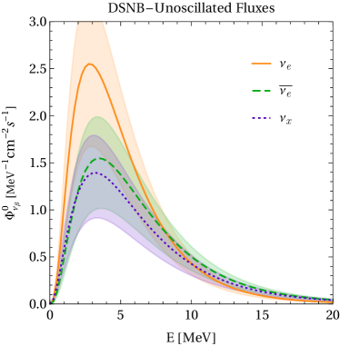
where are the fraction of CC and BH-forming explosions, and are the time-integrated energy spectra for CCSNe and BHF-SNe. In the following, we take . For the , we have performed a fit of the time-integrated neutrino fluences obtained by the Garching group results from (????) in the form of Eq. (II.5), taking as benchmark the data for for CCSNe and as for BHF-SNe. We present in Fig. 1 the unoscillated fluxes at the Earth, obtained from Eq. (II.6) for (orange), (green dashed), and and the corresponding antineutrinos (purple dotted). The flux is about twice the flux at MeV. This difference arises mainly due to the interactions with neutrons that render the average energy of the flux smaller. Meanwhile, the and have closer average energies, making the fluxes much more similar. Such difference will be crucial in our scenario of mass-varying neutrinos.
The neutrino flux gets processed through oscillation effects inside the SN and on the way to Earth. In this study, we neglect the effects of collective neutrino oscillations arising out of neutrino self-interactions deep inside the SN Duan et al. (2006); Hannestad et al. (2006). The quantitative impact of collective oscillations is inconclusive to date, and we expect it to be relatively smaller for neutrinos predominantly produced in the cooling phase. The neutrino flux gets affected by adiabatic Mikheyev-Smirnov-Wolfenstein (MSW) resonant flavor conversion Wolfenstein (1978); Mikheev and Smirnov (1985). Assuming NO, this implies that the are primarily emitted as , while the non-electron neutrinos are emitted as combinations of and . In this case, the final flux at the Earth is given by
| (II.8) |
where , and is the Pontecorvo-Maki-Nakagawa-Sakata (PMNS) mixing matrix. Clearly, the DSNB flux depends on the underlying neutrino oscillation scenario. For example, if the neutrinos were massless at the time of the SN, the flavor evolution of the and (and the antineutrinos) would be trivial inside the explosion. On their way here, these would start oscillating, fast, once the neutrino masses turn on. In this case, the probability that a is detected as a at the Earth is
| (II.9) |
Since SN neutrino energies are smaller than the muon mass, it is convenient to define so
| (II.10) |
In the next sections, we discuss in detail how the DSNB is modified if a fraction of it comes from neutrinos that were “born” with smaller masses or different mixing parameters.
III Mass Varying neutrinos
Following Koksbang and Hannestad (2017); Dvali and Funcke (2016); Lorenz et al. (2019), we assume that the neutrinos remain practically massless down to a certain redshift and gain a non-zero mass for . We further assume the neutrino mass reaches its current value over a finite transition period. This could happen due to neutrinos coupling to the gravitational- term, causing a late phase transition in the Universe Dvali and Funcke (2016), or to neutrinos coupled to a scalar background, which evolves as a function of time Fardon et al. (2004); Berlin (2016); Krnjaic et al. (2018); Dev et al. (2021). Here, we remain agnostic regarding the details of mass-generation.
Assuming momentarily there is only one neutrino mass, we propose that it varies as a function of redshift according to
| (III.1) |
where is the current mass of the neutrino, is a parameter which controls the width of the transition from a massless neutrino to a massive neutrino, and is the redshift below which the neutrino mass turns on. The specific form of the function is irrelevant and is chosen just to present a smooth transition to a non-zero mass. The values of and determine when and at what rate the neutrino mass turns on.
Since there are three neutrino masses, it is possible that they would “turn on” at different and that the transition would be associated to a different value of Bs. Here we assume a universal value for these two phenomenological paramaters. It is also possible to imagine that, as the neutrino mass turns on at , so do all the PMNS mixing angles , and that these turn on in a way that is also captured by Eq. (III.1). We will discuss this possibility later but remain agnostic about the origin of such variations.
In the next section, we will detail the impact of redshift-dependent neutrino masses and mixing angles on the flavor evolution of neutrinos within the SN, as well as from the SN to Earth.
IV Impact of mass varying neutrinos on the DSNB
IV.1 Only masses
We first consider the case where the neutrino masses vary as a function of red-shift while the elements of the mixing matrix are time independent.
IV.1.1 Calculation of the survival probability
In the standard three-massive-neutrinos paradigm, neutrinos produced via charged-current weak interactions are described as superpositions of the three neutrinos with well defined masses, , , . During propagation, the fact that the neutrino masses are different leads the neutrino flavor to oscillate; the associated oscillation lengths are inversely proportional to the differences of the squares of the neutrino masses. Global analysis of the present data indicate that the two independent mass-squared differences are and (plus for NO, minus for IO) Esteban et al. (2020). In matter, the neutrino flavor evolution is modified by the forward elastic neutrino–electron interaction amplitude along the neutrino path.***As mentioned earlier, we will ignore collective effects throughout. This interaction is captured by a matter potential and modifies the effective Hamiltonian that describes neutrino flavor evolution Wolfenstein (1978); Mikheyev and Smirnov (1985). The matter potential depends on the electron number density () along the neutrino path. For position-dependent matter potentials, flavor evolution is rather involved. For certain matter profiles, however, the phenomenon is well understood Parke (1986); Petcov (1988); Krastev and Petcov (1988); Petcov (1988); Friedland (2001). The case where neutrinos are produced in a region of space where is large and propagate towards in the direction where falls roughly exponentially is well known and applies to both solar neutrinos and neutrinos produced in the core of SN explosions.
In the limit where , where is the Fermi constant, is much larger than , where is the neutrino energy and are the neutrino mass-squared differences, electron neutrinos coincide with one of the propagation-Hamiltonian eigenstates (the one with the largest eigenvalue) in the production region. If neutrino flavor evolution is adiabatic inside the medium, the electron neutrino exits the matter distribution as a mass-eigenstate (eigenstate of the flavor-evolution Hamiltonian in vaccum). This “mapping” between the electron neutrino and mass-eigenstates depends on the mass ordering and whether we are considering electron neutrinos or antineutrinos, keeping in mind that the matter potential is positive for neutrinos, negative for antineutrinos.
Given what we know about the mass-squared differences, electron neutrinos, if the flavor evolution inside the SN is adiabatic, exit the SN as for NO and for IO. Electron antineutrinos, instead, exit the SN as for NO and for IO. In the adiabatic regime, it is easy to generalize this picture to the case where is not much larger than one or both : the flavor evolution along the matter potential is just described by the effective mixing parameters at neutrino production.
In the case of two neutrino flavors, if the electron number density decreases roughly exponentially, adiabaticity is controlled by the “crossing probability” . When vanishes, the flavor evolution is perfectly adiabatic. given by Petcov (1988); Krastev and Petcov (1988); Petcov (1988)
| (IV.1) |
where F depends on the matter distribution inside the supernova and the mixing angle Kuo and Pantaleone (1989). The dependence of on the oscillation parameters and is controlled by , which takes the following expression around the resonant region, defined by values that satisfy .
| (IV.2) |
If the variation of the effective mixing angles with the electron number density is slower than the oscillation wavelength in matter, and the neutrino evolution is adiabatic.
It is easy to generalize the discussion to three flavors, taking advantage of the fact that the magnitudes of the two known mass-squared differences differ by two orders of magnitude. In this case, one can define two resonance regions and two crossing probabilities: ( for high), associated to and and ( for low), associated to and . In our computations, in the standard case and NO, we use, for , and and, for , and Esteban et al. (2020).
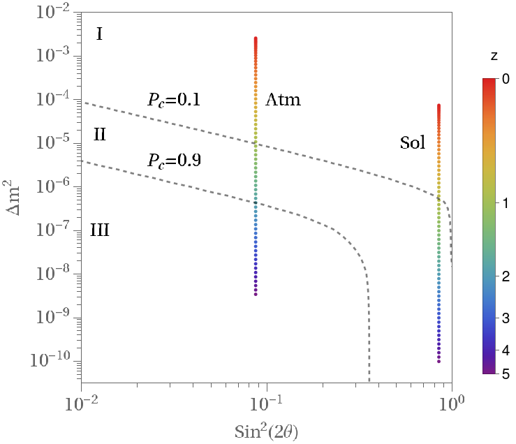
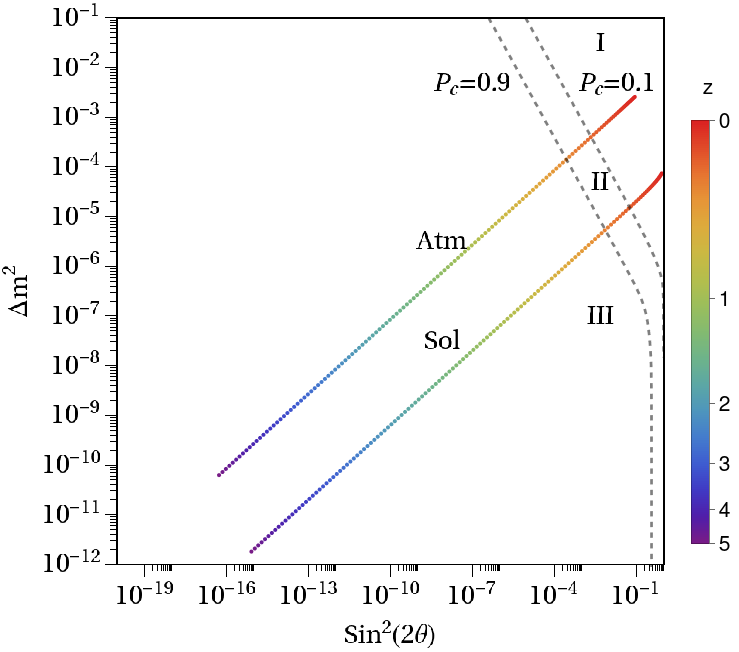
The flavor-at-production and the neutrino spectrum emitted by the supernova depends on the evolution of the collapse of the star. After the shock-wave, free electrons are captured by free protons generated by the dissociation of nuclei yielding a -rich flux – the neutronization burst. Thereafter, a large fraction of the neutrinos are emitted during the cooling phase when the supernova loses the remaining gravitation binding energy via the thermal emission of neutrinos of all flavors. In this phase, the temperature of is expected to be smaller than that of and that of , since interacts more strongly with the production medium. Most of the neutrinos are created deep inside the explosion where the density is quite large. On their way out, neutrinos cross both the atmospheric (), and the solar resonances () at lower densities. Both resonances happen well outside of the neutrinospheres. In Fig. 2, we depict contours of constant in the -plane. We identify three qualitatively distinct regions: (I) , where flavor-evolution “through” the resonance is adiabatic, (II) (region II), and (III) , where neutrino flavor-evolution is highly non-adiabatic. Given the current values of the mass-squared differences ( in the figure), flavor-evolution is very adiabatic through both the atmospheric and solar resonances Dighe and Smirnov (2000). The large value of the density in the region where the neutrinos are produced leads to, as discussed earlier, being mapped to the most massive state (e.g. for NO) while the is mapped into the lighter states (e.g., for NO, some combination of and ). In this case, for NO, the flux of electron neutrinos at the Earth is given by the projection of the three massive states weighted by the initial flux – Eq. (II.8). The small value of implies that most of the at the Earth started out as a deep inside the explosion.
If the neutrino masses were smaller at a given time in the history of the Universe, the flavor evolution inside the supernova might no longer be adiabatic. This is depicted in Fig. 2, where we indicate the different values of the mass-squared differences for different redshifts, following Eq. (III.1) with and . This allows the possibility that one massive state “flip” into another one as the neutrinos propagate through the supernova. In the case of a non-adiabatic evolution and NO, the initial component of the flux will also be partially mapped to and fluxes outside the SN. Following Dighe and Smirnov (2000), the flux at the Earth in the case of a non-adiabatic evolution is given by Eq. (II.10) where the survival probability is given by
| (IV.3) |
In the adiabatic limit (), we recover the standard expression for the flux at the Earth, Eq. (II.8). As the neutrino masses decrease, the atmospheric and solar resonances shift to lower densities. Note that, if the neutrino mass is low enough, the neutrinos might not “cross” one of the resonances on their way out of the SN. That will also impact the final flux.
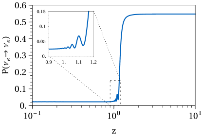
In the case of the normal mass ordering, the non-adiabatic evolution leads to an enhancement of the flux because the initial flux is larger than that of the other flavors. Fig. 3 depicts the electron-neutrino survival probability on the Earth as a function of the redshift of the SN, for MeV, and . For this choice of mass-varying parameters, the transition between massless and massive neutrinos happens around . If the neutrino energy increases, the transition shifts to lower redshifts. Around , we observe a small oscillatory pattern in , highlighted in the inset. For those values of , eV2 and the associated oscillation length is of order the size of the SN.
IV.1.2 The DSNB flux on Earth
In order to include the possibility that neutrino masses are redshift-dependent, Eq. (II.8) needs to be altered:
| (IV.4a) | ||||
| (IV.4b) | ||||
| (IV.4c) | ||||
where, for clarity, we omitted the dependence of on . () indicate the oscillation probabilities for neutrinos (antineutrinos) from a SN explosion at a redshift as described in the last subsection. It depends on the parameters, so the final DSNB flux will contain information regarding them. The DSNB is an integrated flux, so, in principle, there is no an explicit way to distinguish neutrinos that were emitted at higher redshifts from those produced more recently. However, the energies of the neutrinos produced earlier are more redshifted and hence we expect that time-dependent neutrino masses will distort the DSNB energy spectrum.
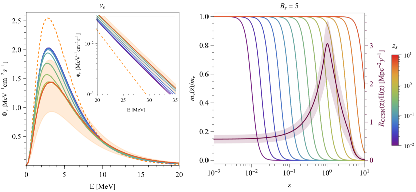
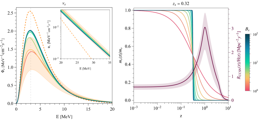
We first consider the case where only the neutrino masses change over time, assuming the NO. Fig. 4, left, depicts the electron neutrino flux at the Earth for different values of , for . The standard flux, for constant neutrino masses, including uncertainties associated to the SFR, is depicted as the orange band while the dashed orange line corresponds to the unoscillated DSNB flux, (i.e., expectations in the scenario where all neutrino masses are exactly zero). We observe that the hypothesis that neutrino masses depend on the redshift can significantly impact the DSNB electron-neutrino flux for . In fact, for , the DSNB flux can be larger than standard expectations by a factor of order for . Moreover, from a simple flux conservation argument, this also implies that the flux at larger energies is reduced with respect to the standard case, see the inset plot. Such neutrinos would have acquired their masses rather recently, when the Universe was old (compare with the age of the Universe ), therefore the DSNB was mostly produced when neutrinos were virtually massless. The increment on the flux at low energies is directly related to the difference between the unoscillated and fluxes. In the standard scenario , so the flux at the Earth is basically the flux produced at the neutrinosphere, which is much broader in energy. However, if significantly differs from the standard case, the contribution from the flux that exited the neutrinosphere becomes significant, thus modifying the flux at the Earth.
For values of , the flux is still larger than the SM flux at low energies. Meanwhile, for , the DSNB flux is basically indistinguishable from the standard case. To understand the dependence on the values of , we show in the right panel of Fig. 4 the redshift evolution of neutrino masses along with the factor , cf. Eq. (II.6). This object describes the SN neutrino production as a function of redshift, including effects associated to the expansion of the Universe. It reveals that most of the DSNB flux is produced at . Thus, if , the SNe matter effects are basically the same as in the standard case, so we do not expect any impact from the mass-varying hypothesis. On the other hand, if , a significant fraction of the DNSB comes from SN explosions that happened when the neutrino masses were significantly smaller. The largest effects occur when neutrinos were effectively massless during most of the history of the Universe, , as noted above.
Fig. 5 captures the dependence of the DSNB flux on the parameter for a fixed . controls how fast neutrino masses increase, larger values associated to more abrupt transitions. For , the transition is almost instantaneous. Whenever the growth of neutrino masses is rapid () the flux is relatively larger (by the same factor, discussed earlier, ). This dependence on again is understood by comparing the redshift dependence of both and (right panel). If the masses become non-zero instantaneously, neutrinos emitted before the transition () would have been effectively massless, and their contribution to the flux will be associated to the electron neutrino survival probability , characteristic of electron neutrinos propagating very long distances in vacuum. After the masses “turn on,” neutrinos will be subject to matter effects inside the SN and in the NO, as discussed earlier. The final DSNB flux will be an amalgam of neutrinos from two different epochs whose contributions are weighted by the SFR divided by the expansion rate. If the transition is not instantaneous (small Bs), the DSNB flux is reduced because matter effects would impact the propagation inside the SN for a longer period of time and the neutrino masses would be of order the current masses for an extended range of redshifts (when the neutrino masses are of the masses today, the matter effects are very similar to the standard case.). Thence, the DSNB flux in such cases is closer to the standard case, as can be observed in Fig. 5.
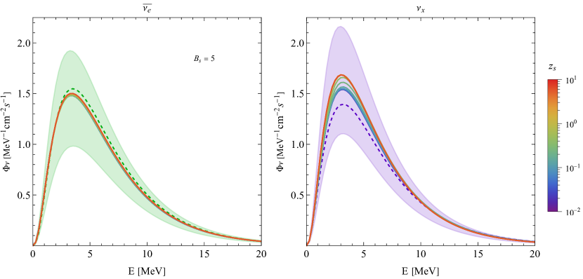
So far, we have focused on the impact of redshift-dependent neutrino masses on the flux assuming NO. Instead the impact on the spectrum is minimal. This is depicted in Fig. 6, left, for NO. This indifference is not strongly dependent on the mass ordering and is mostly a consequence of the fact that the original and fluxes (keeping in mind that includes the antineutrino flavors) are very similar, see Fig. 1. In this case, oscillation effects are invisible. Nonetheless, it is worth discussing the oscillation of in a little more detail. The standard prediction assuming adiabatic propagation indicates that emerges from the SN as so at low energies. The flux at the Earth is, therefore, roughly an equal admixture of and , fluxes that are close to each other. Furthermore, if neutrino masses arise later in the evolution of the Universe (), as in the case. The difference between these fluxes is safely within the star-formation-rate uncertainty, making the effect unobservable, even in the most optimistic cases. Similarly, , measurable only via NC interactions at these low energies, is also modified in a negligible way, as can be observed in the right panel of Fig. 6, for NO. Since it contains the contributions of both neutrinos and antineutrinos, the modification of this flux is at most , within the star-formation-rate uncertainty.
For the IO, the situation changes significantly for . In the standard scenario, the MSW effect predicts that the a created at the neutrinosphere leaves the SNe as a mass eigenstate, so . Meanwhile, if neutrinos only acquired their masses recently (), we would have the same probability as in the NO, . Thus, we find that any possible modification on the DSNB energy spectrum in the IO will lie within the current star-formation uncertainty band. On the other hand, for antineutrinos and the IO, we have , so, if matter effects inside the SNe were significantly different at some point of the evolution of the Universe, would be considerably different from the standard value. Nevertheless, since and are very similar, cf. Fig. 1, any imprint of the mass-varying hypothesis would be very difficult to measure.
IV.2 Masses and mixing
If one allows for the possibility that the neutrino masses are redshfit-dependent, it is reasonable to ask whether the the neutrino mixing parameters also depend on the redshift. We address this possibility in this subsection.
IV.2.1 Calculation of the survival probability
In the case where both the neutrino masses and the mixing parameters depend on the redshift, the adiabaticity of the neutrino flavor-evolution inside the SN is modified relative to the case where only the masses depend on the redshift. Similar to Fig. 2, Fig. 7 depicts contours of constant in the -plane along with the -dependent values of the oscillation parameters. Here, however, both the masses and mixing angles go to zero as grows. Explicitly, we postulate that the redshit-dependent mixing angles , are
| (IV.5) |
Similar to the mass varying scenario, the non-adiabatic evolution of the neutrinos for smaller masses and mixing angles will lead to an enhancement of the flux in the Earth. The lower values of the mixing parameters imply that the flavor resonances happen at lower electron number densities. The minimum densities considered here are around . If the MSW resonance happens at lower densities, neutrinos will not “cross” them as they exit the supernova. In this case, flavor-evolution resembles the vacuum case Friedland (2000). For and , this happens for for the “atmospheric” resonance and for the solar one.
IV.2.2 The DSNB flux at Earth
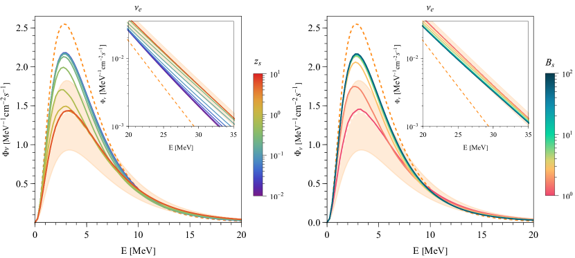
We compute the DNSB flux as discussed around Eq. (IV.4a), this time including in the -dependency of (). As in the previous subsection, we concentrate on the NO and on electron neutrinos, where we anticipate the strongest effects. Similar to the results presented in the last subsection, Fig. 8 depicts the DSNB flux as function of the neutrino energy for different values of . In the left panel, we fix , and vary . In the right panel, we fix , and vary . We observe that the enhancement of at , larger than what we found in the mass-only varying case. At higher energies, instead, the flux is relatively suppressed, by a factor ranging from, roughly, for to at . Hence, the fact that the mixing angles also decrease with increasing redshift leads to more pronounced effects. Taking as example , we find that a emitted at redshifts will exit mostly as a (assuming the normal mass ordering) since the mixing angles are small enough that the PMNS matrix is effectively diagonal. After exiting the supernova, neutrino masses turn on in such a way that they remain a throughout. Thus, at the Earth, the electron survival probability is simply , which enhances the observable flux at lower energies. For the same reason, the flux is suppressed at higher energies MeV, such that, for , the flux lies below the smallest value allowed by the uncertainty on the SFR, see the inset in the left panel.
The dependence on and of the final flux is similar to the masses-only varying case. If , the DSNB is mostly composed of neutrinos that were emitted when their masses and mixing angles where small. On the other hand, if , the largest contribution to the DSNB comes from neutrinos produced with masses and mixing angles similar to the ones observed today. In the latter case, the DSNB will be consistent with standard values. On the other hand, depending on how fast the transition between almost massless neutrinos and the observed mixing pattern occurs, parametrized by , the flux is enhanced at low energies. If the transition is rather sharp (), the DSNB is simply the superposition of a nearly massless component coming from SN explosions with , and a standard part emitted when . For smaller values of , the dependence on redshift is smoother, leading to a small variation of the masses as a function of redshift. For instance, for , and the propagation in the SN is still adiabatic. In this case, there are no significant changes to the DSNB spectrum.
The spectra in this case is virtually unaltered. The MSW adiabatic flavor conversion predicts that , value equal to the probability obtained when the mixing angles are small. Since would be mostly composed by , because the PMNS matrix would be close to diagonal, the predicted antineutrino flux at the Earth would be identical to the standard case. As before, a measurement of both neutrinos and antineutrinos from the DNSB would be crucial to test this scenario.
V Event Spectra in a DUNE-like detector
The detection of the DSNB is one of the main goals of current and future experiments, including SK and HK Abe et al. (2021, 2018), JUNO An et al. (2016), and DUNE Abi et al. (2020). Our results from the last section can be summarized as follows. If the neutrino mass varies as a function of redshift around and if the neutrino mass ordering is normal, we expect the DNSB flux to be very different from standard expectations. The DSNB flux, on the other hand, is quite indifferent to the potential -dependency of neutrino masses. These two facts point towards a simple strategy for testing the hypothesis that neutrino masses “turn on” as a function of time. The detection of the DSNB flux in experiments like SK and HK,†††These experiments, along with scintillator experiments, predominantly detect the DSNB via inverse beta-decay. can be used to normalize the total flux, thus reducing systematic uncertainties, including those related to uncertainties in the SFR. Meanwhile, data from an experiment like DUNE, which can detect electron neutrinos instead of antineutrinos, can be used to provide information on whether the spectrum is consistent with standard expectations.
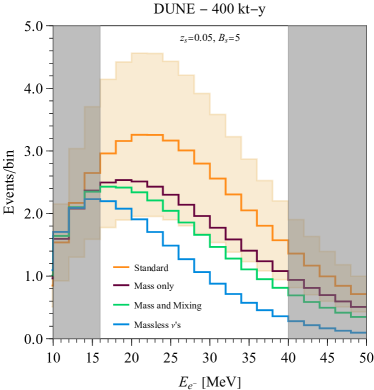
Of course, a measurement of the DSNB in either Cherenkov or Liquid Argon detectors is not an easy task. There are many sources of uncertainty and backgrounds that will impact the search for the DSNB. We do not address these in any detail here but instead, provide a simple example. We compute the number of events at a DUNE-like detector fixing , assuming an exposure of 400 kton-years, and considering as detection channel the process . As far as other characteristics of the DUNE-like detector, we repeat the assumptions we made in Ref. de Gouvêa et al. (2020). Fig. 9 depicts event spectra as a function of the electron kinetic energy. The standard case is depicted in orange along with the uncertainties associated to our imperfect understanding of the SFR (orange region). We consider the case where only the neutrino masses vary (Tyrian purple) and the one where both the masses and mixing angles vary (green). The blue curve corresponds to the expected flux under the assumption that the neutrinos are massless. The gray bands correspond to regions where background events are expected to be dominant. If the neutrino masses “turn on” at a finite redshift, the DSNB flux is significantly smaller relative to standard expectations, as observed in the previous section. For MeV, in the case where both masses and mixing angles vary (green), the flux is expected to lie slightly below the orange-shaded standard region. Fig. 9 reveals that a better understanding of systematic uncertainties is crucial to test the hypothesis that the neutrino oscillation parameters is -dependent. As previously mentioned, a high-statistics measurement of the DSNB antineutrino flux should play a decisive role in reducing uncertainties.
VI Conclusions
After more than two decades, the mystery surrounding the origin of the neutrino mass persists. A popular direction to pursue is to introduce new physics at high or very high energy scales but it is clear that very light new physics can also do the job. There is the possibility that the neutrinos are effectively massless at high redshifts and gain masses only recently, at very low redshifts, due to some exotic new physics operating at these scales. Such low-scale physics only affects the evolution of the Universe after photon decoupling and hence is completely compatible with observations of the CMB and other cosmic surveys.
In this work, we propose that imprints of such low redshift neutrino-mass generation can be found on the diffuse supernova neutrino background (DSNB). The DSNB consists of neutrinos from all past supernovae (SNe), since the birth of star formation (redshifts around ). If neutrino masses are generated at relatively low redshifts, neutrino flavor-evolution through the SN is different from standard expectations. These effects can lead to significant changes to the flavor content of the neutrinos arriving at the Earth. Using a phenomenological parametrization for the redshift evolution of neutrino masses and mixing angles, we computed the DSNB spectra at the Earth. We found that the DSNB spectral shape is sensitive to the epoch of neutrino mass generation: the peak can be, roughly, larger by up to a factor , while the tail can be suppressed, leading to a more pinched spectrum. We also identified scenarios where, earlier in the history of the Universe, neutrino flavor propagation is completely non-adiabatic inside the SN. Finally, we simulated DSNB event spectra in a DUNE-like detector for different hypotheses concerning the time-dependency of the neutrino oscillation parameters and demonstrated that redshift-varying neutrino masses and mixing angles can lead to the suppression of the event spectrum. We find that there are circumstances under which effects due to time-dependent oscillation parameters are significant even if one includes uncertainties associated with our current understanding of the SFR, especially in the higher energy bins. The concurrent measurement, with enough statistics, of both electron neutrinos and antineutrinos from the DSNB, should allow one to make relatively robust claims about the constancy of neutrino masses.
Measurements of the DSNB are possibly the only way to test scenarios where the mass-generation of neutrinos occurred only recently in the history of the Universe. The Super-Kamiokande experiment, doped with gadolinium, is expected to make a compelling discovery of the DSNB within this decade Abe et al. (2021). Future experiments like Hyper-Kamiokande (also doped with gadolinium) and DUNE are expected to collect a significant sample of DSNB events. On the astrophysical front, we expect the uncertainties on the SFR to go down in the coming decades. As a result, it is exciting to wonder whether a measurement of the DSNB can shed some light on the origin of the neutrino mass.
Acknowledgements
We would like to thank Pedro Machado for illuminating discussions on mass-varying neutrinos. IMS, YFPG, and MS would like thank Northwestern University where part of the work was done. IMS and YFPG would like to thank the Fermilab theory group where this work started and for the lovely years well spent there. This work was supported in part by the US Department of Energy (DOE) grant #de-sc0010143 and in part by the National Science Foundation under Grant Nos. PHY-1630782 and PHY-1748958.
References
- Tanabashi et al. (2018) Particle Data Group Collaboration, M. Tanabashi et al., “Review of Particle Physics”, Phys. Rev. D98 (2018), no. 3, 030001.
- Aker et al. (2019) KATRIN Collaboration, M. Aker et al., “Improved Upper Limit on the Neutrino Mass from a Direct Kinematic Method by KATRIN”, Phys. Rev. Lett. 123 (2019), no. 22, 221802, arXiv:1909.06048.
- Aker et al. (2021) M. Aker et al., “First direct neutrino-mass measurement with sub-eV sensitivity”, arXiv:2105.08533.
- Esteban et al. (2020) I. Esteban, M. C. Gonzalez-Garcia, M. Maltoni, T. Schwetz, and A. Zhou, “The fate of hints: updated global analysis of three-flavor neutrino oscillations”, JHEP 09 (2020) 178, arXiv:2007.14792.
- Abbott et al. (2022) DES Collaboration, T. M. C. Abbott et al., “Dark Energy Survey Year 3 results: Cosmological constraints from galaxy clustering and weak lensing”, Phys. Rev. D 105 (2022), no. 2, 023520, arXiv:2105.13549.
- Aghanim et al. (2020) Planck Collaboration, N. Aghanim et al., “Planck 2018 results. VI. Cosmological parameters”, Astron. Astrophys. 641 (2020) A6, arXiv:1807.06209.
- Palanque-Delabrouille et al. (2020) N. Palanque-Delabrouille, C. Yèche, N. Schöneberg, J. Lesgourgues, M. Walther, S. Chabanier, and E. Armengaud, “Hints, neutrino bounds and WDM constraints from SDSS DR14 Lyman- and Planck full-survey data”, JCAP 04 (2020) 038, arXiv:1911.09073.
- Weinberg (1979) S. Weinberg, “Baryon and Lepton Nonconserving Processes”, Phys. Rev. Lett. 43 (1979) 1566–1570.
- de Gouvêa (2016) A. de Gouvêa, “Neutrino Mass Models”, Annual Review of Nuclear and Particle Science 66 (2016), no. 1, 197–217.
- Fardon et al. (2004) R. Fardon, A. E. Nelson, and N. Weiner, “Dark energy from mass varying neutrinos”, JCAP 10 (2004) 005, astro-ph/0309800.
- Krnjaic et al. (2018) G. Krnjaic, P. A. N. Machado, and L. Necib, “Distorted neutrino oscillations from time varying cosmic fields”, Phys. Rev. D 97 (2018), no. 7, 075017, arXiv:1705.06740.
- Dev et al. (2021) A. Dev, P. A. N. Machado, and P. Martínez-Miravé, “Signatures of ultralight dark matter in neutrino oscillation experiments”, JHEP 01 (2021) 094, arXiv:2007.03590.
- Lorenz et al. (2019) C. S. Lorenz, L. Funcke, E. Calabrese, and S. Hannestad, “Time-varying neutrino mass from a supercooled phase transition: current cosmological constraints and impact on the - plane”, Phys. Rev. D 99 (2019), no. 2, 023501, arXiv:1811.01991.
- Dvali and Funcke (2016) G. Dvali and L. Funcke, “Small neutrino masses from gravitational -term”, Phys. Rev. D 93 (2016), no. 11, 113002, arXiv:1602.03191.
- Lorenz et al. (2021) C. S. Lorenz, L. Funcke, M. Löffler, and E. Calabrese, “Reconstruction of the neutrino mass as a function of redshift”, arXiv:2102.13618.
- Formaggio et al. (2021) J. A. Formaggio, A. L. C. de Gouvêa, and R. G. H. Robertson, “Direct Measurements of Neutrino Mass”, Phys. Rept. 914 (2021) 1–54, arXiv:2102.00594.
- Lunardini (2006) C. Lunardini, “The diffuse supernova neutrino flux, supernova rate and sn1987a”, Astropart. Phys. 26 (2006) 190–201, astro-ph/0509233.
- Beacom (2010) J. F. Beacom, “The Diffuse Supernova Neutrino Background”, Ann. Rev. Nucl. Part. Sci. 60 (2010) 439–462, arXiv:1004.3311.
- de Gouvêa et al. (2020) A. de Gouvêa, I. Martinez-Soler, Y. F. Perez-Gonzalez, and M. Sen, “Fundamental physics with the diffuse supernova background neutrinos”, Phys. Rev. D 102 (2020) 123012, arXiv:2007.13748.
- Tabrizi and Horiuchi (2021) Z. Tabrizi and S. Horiuchi, “Flavor Triangle of the Diffuse Supernova Neutrino Background”, JCAP 05 (2021) 011, arXiv:2011.10933.
- Das et al. (2022) A. Das, Y. F. Perez-Gonzalez, and M. Sen, “Neutrino secret self-interactions: a booster shot for the cosmic neutrino background”, arXiv:2204.11885.
- Zhang et al. (2015) Super-Kamiokande Collaboration, H. Zhang et al., “Supernova Relic Neutrino Search with Neutron Tagging at Super-Kamiokande-IV”, Astropart. Phys. 60 (2015) 41–46, arXiv:1311.3738.
- Abe et al. (2021) Super-Kamiokande Collaboration, K. Abe et al., “Diffuse supernova neutrino background search at Super-Kamiokande”, Phys. Rev. D 104 (2021), no. 12, 122002, arXiv:2109.11174.
- Abe et al. (2018) Hyper-Kamiokande Collaboration, K. Abe et al., “Hyper-Kamiokande Design Report”, arXiv:1805.04163.
- An et al. (2016) JUNO Collaboration, F. An et al., “Neutrino Physics with JUNO”, J. Phys. G43 (2016), no. 3, 030401, arXiv:1507.05613.
- Abi et al. (2020) DUNE Collaboration, B. Abi et al., “Deep Underground Neutrino Experiment (DUNE), Far Detector Technical Design Report, Volume II DUNE Physics”, arXiv:2002.03005.
- Pattavina et al. (2020) L. Pattavina, N. Ferreiro Iachellini, and I. Tamborra, “Neutrino observatory based on archaeological lead”, Phys. Rev. D 102 (2020), no. 6, 063001, arXiv:2004.06936.
- Suliga et al. (2022) A. M. Suliga, J. F. Beacom, and I. Tamborra, “Towards probing the diffuse supernova neutrino background in all flavors”, Phys. Rev. D 105 (2022), no. 4, 043008, arXiv:2112.09168.
- Baum et al. (2022) S. Baum, F. Capozzi, and S. Horiuchi, “Rocks, Water and Noble Liquids: Unfolding the Flavor Contents of Supernova Neutrinos”, arXiv:2203.12696.
- Hopkins and Beacom (2006) A. M. Hopkins and J. F. Beacom, “On the normalisation of the cosmic star formation history”, Astrophys. J. 651 (2006) 142–154, arXiv:astro-ph/0601463.
- Yuksel et al. (2008) H. Yuksel, M. D. Kistler, J. F. Beacom, and A. M. Hopkins, “Revealing the High-Redshift Star Formation Rate with Gamma-Ray Bursts”, Astrophys. J. 683 (2008) L5–L8, arXiv:0804.4008.
- Horiuchi et al. (2009) S. Horiuchi, J. F. Beacom, and E. Dwek, “The Diffuse Supernova Neutrino Background is detectable in Super-Kamiokande”, Phys. Rev. D79 (2009) 083013, arXiv:0812.3157.
- Salpeter (1955) E. E. Salpeter, “The Luminosity function and stellar evolution”, Astrophys. J. 121 (1955) 161–167.
- Tamborra et al. (2012) I. Tamborra, B. Muller, L. Hudepohl, H.-T. Janka, and G. Raffelt, “High-resolution supernova neutrino spectra represented by a simple fit”, Phys. Rev. D 86 (2012) 125031, arXiv:1211.3920.
- Møller et al. (2018) K. Møller, A. M. Suliga, I. Tamborra, and P. B. Denton, “Measuring the supernova unknowns at the next-generation neutrino telescopes through the diffuse neutrino background”, JCAP 1805 (2018) 066, arXiv:1804.03157.
- Aghanim et al. (2018) Planck Collaboration, N. Aghanim et al., “Planck 2018 results. VI. Cosmological parameters”, arXiv:1807.06209.
- results from (????) results from, “https://wwwmpa.mpa-garching.mpg.de/ccsnarchive/”.
- Duan et al. (2006) H. Duan, G. M. Fuller, J. Carlson, and Y.-Z. Qian, “Simulation of Coherent Non-Linear Neutrino Flavor Transformation in the Supernova Environment. 1. Correlated Neutrino Trajectories”, Phys. Rev. D74 (2006) 105014, arXiv:astro-ph/0606616.
- Hannestad et al. (2006) S. Hannestad, G. G. Raffelt, G. Sigl, and Y. Y. Y. Wong, “Self-induced conversion in dense neutrino gases: Pendulum in flavour space”, Phys. Rev. D74 (2006) 105010, arXiv:astro-ph/0608695, [Erratum: Phys. Rev.D76,029901(2007)].
- Wolfenstein (1978) L. Wolfenstein, “Neutrino oscillations in matter”, Phys. Rev. D 17 May (1978) 2369–2374.
- Mikheev and Smirnov (1985) S. P. Mikheev and A. Yu. Smirnov, “Resonance Amplification of Oscillations in Matter and Spectroscopy of Solar Neutrinos”, Sov. J. Nucl. Phys. 42 (1985) 913–917, [Yad. Fiz.42,1441(1985)].
- Koksbang and Hannestad (2017) S. M. Koksbang and S. Hannestad, “Constraining dynamical neutrino mass generation with cosmological data”, JCAP 09 (2017) 014, arXiv:1707.02579.
- Berlin (2016) A. Berlin, “Neutrino Oscillations as a Probe of Light Scalar Dark Matter”, Phys. Rev. Lett. 117 (2016), no. 23, 231801, arXiv:1608.01307.
- Wolfenstein (1978) L. Wolfenstein, “Neutrino Oscillations in Matter”, Phys. Rev. D 17 (1978) 2369–2374.
- Mikheyev and Smirnov (1985) S. P. Mikheyev and A. Y. Smirnov, “Resonance Amplification of Oscillations in Matter and Spectroscopy of Solar Neutrinos”, Sov. J. Nucl. Phys. 42 (1985) 913–917.
- Parke (1986) S. J. Parke, “Nonadiabatic Level Crossing in Resonant Neutrino Oscillations”, Phys. Rev. Lett. 57 (1986) 1275–1278.
- Petcov (1988) S. T. Petcov, “Exact analytic description of two neutrino oscillations in matter with exponentially varying density”, Phys. Lett. B 200 (1988) 373–379.
- Krastev and Petcov (1988) P. I. Krastev and S. T. Petcov, “On the Analytic Description of Two Neutrino Transitions of Solar Neutrinos in the Sun”, Phys. Lett. B 207 (1988) 64, [Erratum: Phys.Lett.B 214, 661 (1988)].
- Petcov (1988) S. T. Petcov, “On the Oscillations of Solar Neutrinos in the Sun”, Phys. Lett. B 214 (1988) 139–146.
- Friedland (2001) A. Friedland, “On the evolution of the neutrino state inside the sun”, Phys. Rev. D 64 (2001) 013008, hep-ph/0010231.
- Kuo and Pantaleone (1989) T.-K. Kuo and J. T. Pantaleone, “Nonadiabatic Neutrino Oscillations in Matter”, Phys. Rev. D 39 (1989) 1930.
- Dighe and Smirnov (2000) A. S. Dighe and A. Yu. Smirnov, “Identifying the neutrino mass spectrum from the neutrino burst from a supernova”, Phys. Rev. D62 (2000) 033007, arXiv:hep-ph/9907423.
- Friedland (2000) A. Friedland, “MSW effects in vacuum oscillations”, Phys. Rev. Lett. 85 (2000) 936–939, hep-ph/0002063.
- Abe et al. (2021) Super-Kamiokande Collaboration, K. Abe et al., “First Gadolinium Loading to Super-Kamiokande”, arXiv:2109.00360.
- Abe et al. (2018) Hyper-Kamiokande Collaboration, K. Abe et al., “Hyper-Kamiokande Design Report”, arXiv:1805.04163.
- An et al. (2016) JUNO Collaboration, F. An et al., “Neutrino Physics with JUNO”, J. Phys. G 43 (2016), no. 3, 030401, arXiv:1507.05613.
- Abi et al. (2020) DUNE Collaboration, B. Abi et al., “Deep Underground Neutrino Experiment (DUNE), Far Detector Technical Design Report, Volume I Introduction to DUNE”, JINST 15 (2020), no. 08, T08008, arXiv:2002.02967.