Article Title

Coordination-free Multi-robot Path Planning for Congestion Reduction Using Topological Reasoning

Abstract

We consider the problem of multi-robot path planning in a complex, cluttered environment with the aim of reducing overall congestion in the environment, while avoiding any inter-robot communication or coordination. Such limitations may exist due to lack of communication or due to privacy restrictions (for example, autonomous vehicles may not want to share their locations or intents with other vehicles or even to a central server). The key insight that allows us to solve this problem is to stochastically distribute the robots across different routes in the environment by assigning them paths in different topologically distinct classes, so as to lower congestion and the overall travel time for all robots in the environment. We outline the computation of topologically distinct paths in a spatio-temporal configuration space and propose methods for the stochastic assignment of paths to the robots. A fast replanning algorithm and a potential field based controller allow robots to avoid collision with nearby agents while following the assigned path. Our simulation and experiment results show a significant advantage over shortest path following under such a coordination-free setup.

1 Introduction

1.1 Motivation and Problem Description

Autonomous vehicles are expected to travel in urban environments in the future for increased safety and overall efficiency. They could be of different car brands running different navigation & communication systems that do not share their route-choosing processes or travel data, either due to lack of communication or due to privacy restrictions. To avoid traffic congestion, such as those caused by non-cooperating human drivers nowadays, independent autonomous vehicles need to have a method for distributing traffic in the environment without communication. Motivated by this real-world scenario, in this paper we consider the problem of path planning for a large number of privacy-aware robots in a complex, cluttered indoor or urban environment with uncertainties (other unpredictable agents such as pedestrians), where the robots need to be well-distributed throughout the environment and avoid congestion in any region, but are not allowed to communicate or share their location data or intents with other robots. This is relevant to avoiding congestion in distributed vehicle routing problems when a vehicle’s location/intent cannot be shared either due to lack of communication or due to privacy restrictions. We address the fundamental question of

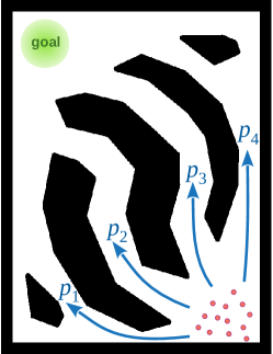
Figure 1: Key idea: Make each robot stochastically choose from a set of topologically distinct paths in the environment.

path planning under such circumstances without any inter-robot coordination, while trying to minimize the overall congestion in the environment. We assume that each robot knows the map of the environment and can localize itself in it, but do not know the location or intent of the other robots. Furthermore, a robot can detect other agents in its immediate neighborhood (for example using on-board cameras or laser range sensors) so as to be able to avoid immediate collisions with them, although they cannot broadcast or communicate any information with each other. The key insight that allows us to solve this problem is to make each robot stochastically choose from a set of different routes in the environment which correspond to paths in different topologically distinct classes (Figure 1), so as to lower congestion and the overall travel time for all robots in the environment.

1.2 Literature Review

MAPF: Multi-agent path finding (MAPF) is a well-studied problem with a variety of practical applications. Given a set of robots and their start locations, the objective of MAPF is to find a set of paths that lead them to their corresponding goals without collision, while minimize the sum of travel time of each agent. Early studies (silver2005cooperative, ) focused on computing valid collision-free solutions, while recent method (sharon2015conflict, ) and its many variants have strived to compute optimal solutions. They all focus on conflict resolution among the agents’ path choices so that an optimal or near-optimal solution can be achieved. Furthermore, existing algorithms (han2020ddm, ; wagner2011m, ) are designed to deal with agents that are well-distributed across the environment and not have similar start/goal locations. For example, in  han2020ddm , in all presented results, the initial robot positions are chosen to be distributed uniformly throughout the environment. For a large group of robots with similar start and goal points, the computation involved in existing MAPF methods will increase drastically due to increased collision avoidance computations, and the collision/congestion avoidance still happens at a local level.

MAPF in dynamic, cluttered and uncertain environments is also well-studied in robotics (MOHANAN2018171, ; Kushleyev:09, ; 2020arXiv200614195C, ; Hasan:18, ). Such dynamic environments exist in presence of pedestrians and other robots in busy indoor or urban environments. Robots employed in such environments need to arrive at designated target locations while avoiding both static and dynamic obstacles such as pedestrians, which is usually unknown to the path planner at the first place. The dynamic nature of the environment in all these existing work, however (see the review paper 2020arXiv200614195C for example), is assumed to arises from completely unpredictable agents (both human pedestrians and other robots), and hence these work focus primarily on improving the short-term prediction of the behavior of such agents without consideration for long-term congestion reduction. We, on the other hand, consider the problem where the robots in the environment use the same stochastic algorithm that, even without inter-agent coordination or communication, results in overall reduction of congestion in the environment in the long-term.

Along similar lines, some studies (ziebart2009planning, ; kretzschmar2016socially, ) have focused more on pedestrian’s trajectory prediction or social compliance with humans that facilitate obstacle avoidance in a more human-friendly way, but is still at a local level and over short time horizons. Over longer time periods, when multi-robot groups run on a large complicated map cluttered by dynamic obstacles, this does not help proactively avoid robot congestion in the long run if the robots’ routes are not well-distributed across the environment. In this paper we focus on developing algorithms for individual robots that, even without inter-robot communication or coordination, tries to reduce overall congestion in the environment by stochastically distributing the robots over different routes.

While the presence of uncertain agents such as pedestrians in such planning problems have been considered (kirby2009companion, ; sisbot2007human, ; ferrer2013social, ; shiomi2014towards, ), the problem of reducing robot traffic congestion by taking advantage of the structure of the environment without explicit inter-robot coordination remains open.

Congestion Avoidance in MAPF: Both with and without uncertainties, existing literature uses inter-robot coordination for global planning to avoid congestion (atzmon2020probabilistic, ; santos2011hierarchical, ; toutouh2018swarm, ; ANTONIOU20131167, ), or use information stored in the environment (represented as a network) as a means of indirect coordination between the agents (1706747, ; gunes2002ara, ; di2005anthocnet, ). A recent work on congestion-aware policy synthesis (street2021congestion, ) is notable, and tries to achieve a balance between congestion reduction and minimization of detours by designing single-robot automata. However, even in this approach, significant centralized inter-robot coordination (using a shared probabilistic reservation table) is necessary. This assumption of inter-robot coordination is fundamentally different from the premise of our current work, where we assume that there exists no inter-agent communication or coordination, and robots do not share their plan or intent. Furthermore, (street2021congestion, ) does not consider out-of-system agents (unpredictable agents such as pedestrians), which we do in our current work.

Other Related Multi-robot Coordination Problems: Most multi-robot persistent patrolling/surveillance methods use some centralized coordination (Stump:11:surveillance, ; Leahy:Surveillance:16, ; Kusnur_muav_19, ; Thakur-2013-109538, ). In a inter-robot communication denied situation, local methods (e.g., repulsive force or velocity obstacle (van2008reciprocal, )) or other decentralized framework (using topological braids (mavrogiannis2019multi, ) or rotations (mavrogiannis2022winding, )) can only help avoid collision but not avoid congestion proactively. In those methods, without inter-robot coordination, congestion could readily happen. Action strategy planning for robots minimizing expected cost, while a well-researched area (and often addressed using reinforcement learning or game-theoretic methods (lavalle2000robot, ; he2020integral, )), mostly focuses on local actions, do not take global topology of the environment into account, rely on shared information, or do not scale with the number of robots (for example, he2020integral presents results with only three robots).

1.3 Solution Overview and Paper Outline

The technical problem considered in this paper can be summarized as follows:

Problem Statement: Given a discrete graph representation of an environment, how can a large number of privacy-aware robots with local sensing plan their respective paths in the graph without inter-robot communication or centralized coordination (i.e., without sharing their location or intents) so as to minimize the overall congestion in the environment.

If all robots choose the same/similar paths (e.g., shortest paths), certain regions of the environment will inevitably be traversed more. This issue is even more aggravated when the robots or groups of robots have similar start and goal locations. Instead, a robot stochastically chooses between different topologically distinct classes of solutions with an aim of reducing overall congestion in the environment and to altruistically minimize overall travel time for any robot. We leverage the topological path planning methods introduced in the author’s prior works (planning:AURO:12, ; Homotopy-Planning:journal:18, ; Wang:Cable-Controlled:2018, ; DARS:14:HRI, ; Persistence-Plnning:TRO:15, ; ICRA:20:path:deconfliction, ) for computing the topologically distinct paths in the environment.

Contributions: The main new contributions of the paper are:

1. Formulating an optimization problem for coordination/communication-free computation of probability values using which a robot stochastically chooses a path out of the available topologically distinct choices.

2. Develop efficient computation methods for solving the said optimization problem by employing simplifications.

3. Design the controller used by each non-holonomic robot to follow their chosen path while locally avoiding collisions with other agents in its immediate neighborhood. This requires the development of a fast re-planner that takes the topological class into account.

4. Validate the proposed method in simulations and real robot experiments.

Paper Outline: In Section 2 we provide background on the computation of paths in topologically distinct classes using discrete search in $\mathbb{Z}_{2}$-homology augmented graphs. The main contributions of the paper appear in Section 3, where we describe the coordination-free computation of the probability values using which a robot stochastically chooses a path out of the available topologically distinct choices. This includes estimation of traffic density in the environment (Section 3.2), which is used

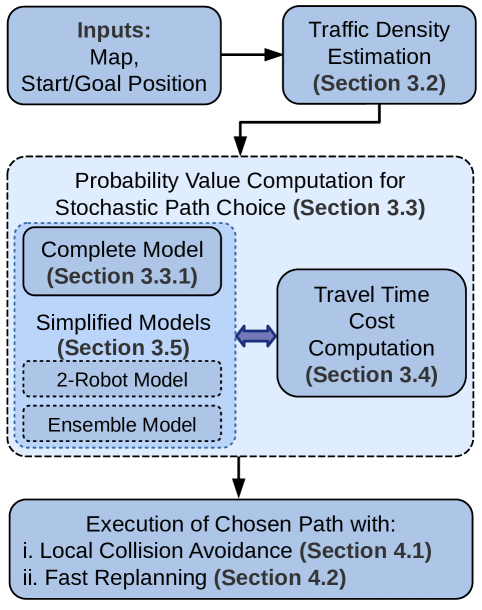
Figure 2: Workflow of the proposed coordination-free planning. Each robot follows this sequence of algorithms for computing and executing its own path without any inter-robot coordination or communication.

in the evaluation of the cost of path choices (Section 3.4), which in turn is used in the computation of the probability values through an optimization process (Section 3.3). We also provide multiple appromixations and simplifications to the optimization problem for fast and efficient computation (Section 3.5). A robot stochastically chooses a path using the computed probability values. We call a chosen path the reference path of the robot, and once chosen, a robot commits to it. Section 4 describes the controller used by each non-holonomic robot to follow the reference path while locally avoiding collisions with other agents in its immediate neighborhood. This includes a prediction of the future position of agents in the immediate neighborhood (Section 4.1) and fast re-planning of path to avoid collision (Section 4.2). Section 5 provides simulation results and results from real-robot experiments.

The overall algorithm that each robot follows in computing and executing their respective paths is shown in the pipeline diagram of Figure 2. The relevnat section numbers containing the details of each of the algorithmic components are also shown in the figure.

2 Preliminaries – Topological Planning and Rationalized Discretization in Spatio-Temporal Domain

In this section we provide brief background on topological path planning that allows the computation of shortest path in different topological classes using a graph search-based approach. For further details on topological path planning the reader can refer to the author’s prior work (planning:AURO:12, ; Homotopy-Planning:journal:18, ; Wang:Cable-Controlled:2018, ; DARS:14:HRI, ). The type of topological classes that we consider in particular is the $\mathbb{Z}_{2}$ homology class (Persistence-Plnning:TRO:15, ; ICRA:20:path:deconfliction, ), and we describe the path planning in spatio-temporal domain in order to account for dynamic agents during replanning.

2.1 Background: $\mathbb{Z}_{2}$ Homology and $H_{2}$-signature

Two trajectories connecting the same start and goal points on a planar domain are said to be in the same homology class if the closed loop formed by the two trajectories forms the oriented boundary of a two-dimensional obstacle-free region (planning:AURO:12, ). The homology class of a loop can be quantified by winding numbers around the connected components of obstacles. In order to prevent the separate counting of the homology classes that loop around an obstacle multiple times, one can compute the homology in the “mod $2$” coefficient (Persistence-Plnning:TRO:15, ; ICRA:20:path:deconfliction, ). Doing so identifies all the even winding numbers to $0$ and all the odd winding numbers to $1$. This prevents the creation of separate homology classes for loops that wind around obstacles multiple times (Figure LABEL:pic:z2homology) and we refer to this homology as $\mathbb{Z}_{2}$-homology.

In order to quantitatively identify and represent $\mathbb{Z}_{2}$-homology class of trajectories in a planar domain, $\mathcal{C}=\mathbb{R}^{2}-\mathcal{O}$ (where $\mathcal{O}\subset\mathbb{R}^{2}$ is the obstacle set), we construct a homology invariant called $H_{2}$-signature, which is a function on the space of curves in $\mathcal{C}$ that uniquely identifies a curve’s $\mathbb{Z}_{2}$-homology class. This computation and the associated construction (see (cable:separation:IJRR:14, ; Persistence-Plnning:TRO:15, ) for more details) can be summarized as follows: In an environment with $o$ connected components of obstacles we place a representative point, $\zeta_{i}$, on the $i^{\text{th}}$ connected component and construct non-intersecting rays, $\{r_{i}\}_{i=1,2\cdots,o}$, emanating from the representative points. The $H$-signature of a curve, $\tau$, is then given by a vector of integers, $H(\tau)=[h_{1},h_{2},\cdots,h_{o}]\in\mathbb{Z}^{o}$, where $h_{i}$ is the winding number around the $i^{\text{th}}$ obstacle and can be computed by the number of times the curve intersects the ray emanating from $\zeta_{i}$ (in counting the number of intersections, crossing from left to right is considered positive and that from right to left is considered negative). Subsequently, the $H_{2}$-signature of $\tau$ is defined as $H_{2}(\tau)=[h_{1},h_{2},\cdots,h_{o}]\mod 2\in\mathbb{Z}_{2}^{o}$, in which the $i^{\text{th}}$ element assumes value in $\mathbb{Z}_{2}=\mathbb{Z}/2\mathbb{Z}=\{0,1\}$ and gives the parity of the number of times the curve intersects the ray emanating from $\zeta_{i}$. This computation is further illustrated in Figure LABEL:pic:z2homology.

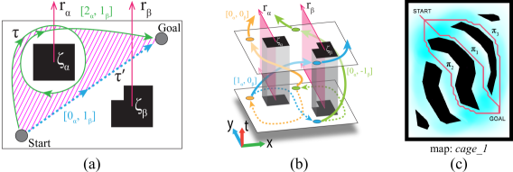
Figure 3: Topological Planning in $H_{2}$-augmented graph: (a) Homology classes of trajectories: $\tau$ and $\tau^{\prime}$ are in different classes in regular homology ($H(\tau)=[2,1],H(\tau^{\prime})=[0,1]$), but map to the same class in $\mathbb{Z}_{2}$-coefficient homology ($H_{2}(\tau)=H_{2}(\tau^{\prime})=[0,1]$), where the elements of the vector are reduced ‘$\!\!\mod 2$’. As a consequence, in computing paths in different homology classes, searching in the $H_{2}$-augmented graph does not return paths that loop around obstacles multiple times. (b) $H_{2}$-signature in a spatio-temporal configuration space. (c) Three paths in different $\mathbb{Z}_{2}$-homology classes (colored in pink) from the start to the goal in map “cage_1” computed using search in the $H_{2}$-augmented graph $\mathcal{G}_{H_{2}}$. Their base costs (travel time cost computed by the A* search) are $\mathscr{C}_{B}(\pi_{1})\!=\!8.803$, $\mathscr{C}_{B}(\pi_{2})\!=\!9.803$, $\mathscr{C}_{B}(\pi_{3})\!=\!10.603$. Cyan shade shows the estimated traffic density, $\rho$ (described in Section 3.2).

2.2 Topological Planning in $H_{2}$-Augmented Graph In Spatio-Temporal Domain

The configuration space of each of the robots in our case is a discrete representation of the spatio-temporal domain. For a single robot, it is represented by the graph, $\mathcal{G}=(\mathcal{V},\mathcal{E})$, so that a vertex $\mathbf{v}\in\mathcal{V}$ is represented by $\mathbf{v}=(x,y,t)$, and edges connect neighboring vertices. In order to keep track of the $\mathbb{Z}_{2}$ homology invariants, we define an $H_{2}$-augmented graph (see (planning:AURO:12, ; cable:separation:IJRR:14, ; Persistence-Plnning:TRO:15, ) for detailed construction), $\mathcal{G}_{H_{2}}=(\mathcal{V}_{H_{2}},\mathcal{E}_{H_{2}})$, based on the graph $\mathcal{G}$, such that a vertex in it is represented as $(\mathbf{v},\mathfrak{H})\in\mathcal{V}_{H_{2}}$, which contains the additional information of the $H_{2}$-signature, $\mathfrak{H}$, of the trajectory leading from a start vertex $\mathbf{v}_{s}\in\mathcal{V}$ up to the vertex $\mathbf{v}$. An edge connecting vertex $(\mathbf{v},\mathfrak{H})$ to vertex $(\mathbf{v}^{\prime},\mathfrak{H}^{\prime})$ exists if $(\mathbf{v},\mathbf{v}^{\prime})\in\mathcal{E}$, and $\mathfrak{H}^{\prime}$ is the sum of $\mathfrak{H}$ and the $H_{2}$-signature of the edge connecting $\mathbf{v}$ to $\mathbf{v}^{\prime}$.

In the spatio-temporal setup the rays in Figure LABEL:pic:z2homology emanating from obstacles are extruded in the temporal direction to construct half-planes (Figure LABEL:pic_Haugmentedspace) and the intersections of trajectories are counted with these half-planes for computing the $H_{2}$-signature. Thus in this case the $H_{2}$-signature computation for a path in the X-Y-T space requires counting the number of intersections of the path with each of those half-planes.

Formally, given the graph, $\mathcal{G}$ and a start vertex $\mathbf{v}_{s}\in\mathcal{V}$, the vertex set, edge set and the cost function of the $H_{2}$-augmented graph can be described as:

1. $(\mathbf{v},\mathbf{0})\in\mathcal{V}_{H_{2}}$ is the start vertex, and the vertex set is given by:

   $$\mathcal{V}_{H_{2}}=\left\{(\mathbf{v},\mathfrak{H})\left|\begin{aligned} &\mathbf{v}\in\mathcal{V},\text{ and},\mathfrak{H}=H_{2}(\widetilde{\mathbf{v}_{s}\mathbf{v}})\\ &\text{ for some trajectory }\widetilde{\mathbf{v}_{s}\mathbf{v}}\\ &\text{from the start vertex }\mathbf{v}_{s}\text{ to }\mathbf{v}\end{aligned}\right.\right\}$$

2. An edge $\{(\mathbf{v},\mathfrak{H})\to(\mathbf{v}^{\prime},\mathfrak{H}^{\prime})\}$ is in $\mathcal{E}_{H_{2}}$ iff $(\mathbf{v}\to\mathbf{v}^{\prime})\in\mathcal{E}$ and $\mathfrak{H}^{\prime}=\left(\mathfrak{H}+H_{2}(\mathbf{v}\to\mathbf{v}^{\prime})\right)\!\!\mod 2$, where, $H_{2}(\mathbf{v}\to\mathbf{v}^{\prime})$ is the $H_{2}$-signature of the directed segment representing the edge $(\mathbf{v}\to\mathbf{v}^{\prime})$, and “$+$” is vector addition.

3. The cost associated with an edge, $C_{\mathcal{G}_{H_{2}}}\left(\{(\mathbf{v},\mathfrak{H})\to(\mathbf{v}^{\prime},\mathfrak{H}^{\prime})\}\right)$ is the same as the cost of the projected edge in, $\mathcal{G}$, i.e., $C_{\mathcal{G}}\left(\{\mathbf{v}\to\mathbf{v}^{\prime}\}\right)$. The cost function is described in more details in Section 2.4.

Searching in this $H_{2}$-augmented graph from the start vertex $(\mathbf{v}_{s},\mathbf{0})$ using A* search Choset_2005 , paths to vertices of the form $(\mathbf{v}_{g},*)$ give paths in different $\mathbb{Z}_{2}$ homology classes connecting $\mathbf{v}_{s}$ and $\mathbf{v}_{g}$ (Figure LABEL:pic_classes). The vertices are generated on-the-fly and as required during the execution of A* search on the graph. The paths obtained in the different homology classes are in ascending order of the cost.

2.3 Rationalized Discretization of the Spatio-Temporal Configuration Space for Constructing $\mathcal{G}$

In order to construct the configuration graph, $\mathcal{G}$, we discretize the spatio-temporal domain into a grid and place a vertex in every discrete cell in the grid. The time axis is discretized uniformly with the time layers separated by $\delta t$ (Figure LABEL:pic_successors_2). In the initial planning for the reference path we assume a constant robot speed, $V_{\text{max}}$, which is difficult to achieve with a uniform spatial discretization of $\delta r=V_{\text{max}}\delta t$ along X and Y directions (since diagonal edges of an uniform square grid discreitization are longer than the edges parallel to the coordinate axes). Instead, we discretize the spatial directions (both X and Y) using intervals of $\delta r^{\prime}=\frac{\delta r}{4}$ and establish edges connecting a vertex $(x,y,t)\in\mathcal{V}$ with vertices of the form $(x\pm 3\delta r^{\prime},y\pm 3\delta r^{\prime},t+\delta t)$, $(x\pm 4\delta r^{\prime},y,t+\delta t)$ and $(x,y\pm 4\delta r^{\prime},t+\delta t)$ (see Figure LABEL:pic_successors_1). In doing so, the spatial length of edges parallel to X or Y axes are $\delta r$, while the spatial length of the diagonal edges are $\sqrt{2}\frac{3}{4}\delta r=1.06\cdots\delta r\approx\delta r$ (Figure LABEL:pic_successors_1), thus allowing the implementation of almost-isotropic (direction-independent) velocity of $V_{\text{max}}$ along the edges. We call this the “Rationalized Discretization”.

Figure 4: Successors (cyan) of a vertex $(x,y,t)\in\mathcal{V}$ (in red) using the rational discretization. Note how, although the successors with different spatial coordinates do not exactly fall on a circle of radius $V_{\text{max}}\delta t$, they do approximate the circle reasonably well due to the rationlized discretization.

2.4 Cost Function and Heuristic Function for A* Search for Computing Paths in Different Topological Classes

For the topological planning of the paths in different $\mathbb{Z}_{2}$-homology classes for a particular robot, the cost function accounts for the traversal time for the edges. The cost of an edge connecting vertices $(x,y,t,\mathfrak{h})$ and $(x^{\prime},y^{\prime},t+\delta t,\mathfrak{h}^{\prime})$ in $\mathcal{E}_{H_{2}}$ is thus chosen to be $\sqrt{(x^{\prime}-x)^{2}+(y^{\prime}-y)^{2}}/V_{\text{max}}$. From a vertex $(x,y,t,\mathfrak{h})$ it will take at least $T_{g}=\frac{\sqrt{(x_{g}-x)^{2}+(y_{g}-y)^{2}}}{V_{\text{max}}}$ time to reach a goal vertex of the form $(x_{g},y_{g},*,*)$ using any $\mathbb{Z}_{2}$ homology class, which is used as the heuristic function for A* search in $\mathcal{G}_{H_{2}}$. An A* search in this $H_{2}$-augmented graph is used to find paths to vertices of the form $(x_{g},y_{g},*,*)$, which returns paths in increasing order of cost, and the cost of a path, $\pi$, is denoted by $\mathscr{C}_{B}(\pi)$, which is referred to as the base travel cost.

3 Stochastic Topological Path Assignment for Coordination-free Multi-robot System

In this section we describe the algorithm that a robot uses for computing the probability values with which it stochastically assigns itself to one of the topologically distinct paths that it has computed. The main consideration in designing the algorithm is that the robots are not allowed to communicate or coordinate among themselves in either the computation of the probability values or in choosing their own path assignments. A robot does not share its location or its intent/choice with other robots. In the next section we start with a brief description of the problem setup and introduce some terminologies.

3.1 The Environment and a Robot’s Mental Model of the Environment

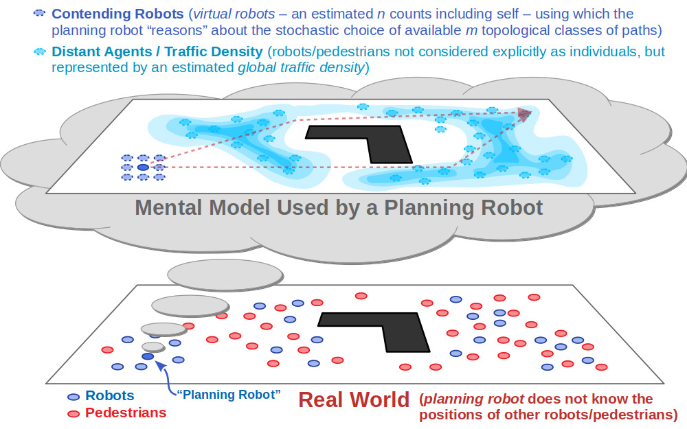
Figure 5: The mental model of a robot computing its own path (a planning robot): In absence of the knowledge of the positions of other robots or pedestrians, a robot reasons about its stochastic choice from the available topological classes of paths using a team of virtual robots with similar start/goal (the “contending robots”). All other agents (robots or pedestrians – referred to as “distant agents”) are accounted by an estimated traffic density map, $\rho$.

We consider a planar indoor or urban environment with multiple robots navigating from one location to another within the environment while trying to avoid global traffic congestion. While the robots are rational agents (their actions are determined by an algorithm that altruistically tries to reduce global traffic congestion), there also exist non-rational agents (pedestrians) that do not attempt to reduce congestion in their path planning. Robots need to maintain a minimum safe distance from other robots as well as pedestrians. Because of that, if a passage or route in the environment becomes too crowded, some may have to slow down or wait for the congestion to reduce. Due to lack of inter-robot coordination, a lack of knowledge of the current global traffic state/distribution in the environment, and the unpredictable nature of the pedestrians, it is virtually impossible to predict such congestion ahead of time. As a consequence, the overall travel time of all robots could increase significantly. The key insight in addressing this problem is to distribute the robots across different routes in the environment so as to lower the probability of congestion. Assigning the robots paths in different topological ($\mathbb{Z}_{2}$ homology) classes in the environment can help achieving that.

3.1.1 Types of Agents and the “Planning Robot”

In the environment we assume that there are two types of agents – i. non-rational agents, also referred to as pedestrians, that always choose the shortest path without consideration for global congestion reduction, and ii. rational agents, also referred to as robots, that stochastically chooses one of the multiple topologically distinct paths available to it with an aim of reducing global congestion. Without coordination between the robots, all computation of the paths and stochastic path selection for a particular robot happen onboard the robot itself in a decentralized manner, without communication with other robots. In the following sections, we describe the computations made by a particular robot (i.e., from the perspective of that individual robot), referred to as “the planning robot”. It is to be noted that all robots are planning robots in their own rights, and the same algorithm is used by each robot for its individual computation.

3.1.2 Decoupling the Problem to Reason About Global Agent Distribution and Local Path Selection

A planning robot needs to not only reason about other robots that may have similar start and goal locations as itself, but also the robots that may have different start/goal locations as well as the pedestrians. Without knowing the location, intent, or choices of other agents in the environment, a planning robot decouples this complex problem into two parts: i. Estimation of global traffic density, $\rho$, in the environment based on a prior belief of agent trajectories (Section 3.2), and, i. Probabilistic choice of topologically distinct paths for avoiding congestion (Sections 3.3–3.5).

A planning robot does not know the location of other agents (pedestrians or other robots) in the environment. In order to reason about the available topological classes connecting its own start and goal locations, it considers a group of virtual robots with similar start & goal locations. These robots are referred to as contending robots, and having similar start/goal locations have the same topological classes of paths as the planning robot and thus enables reasoning about the stochastic choice of a class (Figure 5). Other agents (referred to as distant agents) in the environment are represented by an estimated traffic density map, which is used in evaluating the different topological classes of paths when making the stochastic choice.

3.2 Estimation of Traffic Density in an Environment

Figure 6: Maps used for simulations and experiments. Traffic density maps estimated without a priori knowledge of any historic traffic data are shown using shades of cyan – darker cyan indicates potentially busier traffic regions.

This density estimation not only accounts for pedestrians, but also potentially accounts for robots that have start & goal locations that are widely different from the planning robot. We refer to such agents as distant agents. This density is used in formulating the optimization problem for computing the probability values associated with the different topologically distinct path options available to the planning robot.

The distant agents’ traffic density, $\rho:V\rightarrow\mathbb{R}_{+}$, is described by a real number associated with each cell (pixel) in the discrete representation of the environment. While $\rho$ can be computed from historic traffic data, in absence of such data it can also be estimated from the structure of the environment. In order to do that, traffic is randomly generated with thousands of shortest paths connecting random starts to goals. Then each path is thickened by Minkowski summing it with the pedestrians’ disk-shaped footprint, and for each discrete cell in the map the number of such thickened paths that pass through it is counted. This distribution is then normalized to obtain the density function, $\rho$. Some examples of traffic density maps computed this way are shown in Figure 6. This traffic density is an estimation only, related to the map’s topology and geometry, and needs to be computed only once for a given environment.

3.3 Probabilistic Choice of a Topological Class

In order to avoid congestion along the possible routes that the planning robot can choose to reach its goal, the robot needs to reason about the choices made by other robots that have similar start and goal locations as itself. To that end the robot can choose from multiple topological classes of paths representing distinct routes leading to its goal. However, without coordination between the robots, a probabilistic approach is taken in which the planning robot reasons about an estimated $n$ robots, including itself, with similar start and goal (refereed to as contending robots) and chooses a topological class stochastically based on probability values computed to minimize the travel time for all the contending robots.

The planning robot starts by computing $m$ topologically distinct paths connecting its start to its goal location (Section 2). The paths are referred by by their number/index from the set $S=\{1,2,\dots,m\}$. The planning robot needs to choose one out of these $m$ classes stochastically. Suppose $P_{j}$ is the probability with which the robot chooses the $j$-th path. In order to compute the path choice probabilities, $\{P_{j}\}_{j\in S}$, the robot reasons about the time of travel if all the contending robots choose the paths from $S$ according to the probabilities $\{P_{j}\}_{j\in S}$ (the contending robots being rational agents will use the same probability computation method themselves, thus arriving at the same probability values).

3.3.1 Path Choice Probability Computation – The Complete Formulation

The value of $n$, while unknown, can be estimated based on the a priori knowledge of agent density in the environment or through local sensing. However, the planning robot uses the value $n$ only for the computation of its own path choice probability values $\{P_{j}\}_{j\in S}$, while in reality there is no real coordination between the planing robot and the other robots.

We denote the set of contending robots as $R=\{1,2,\cdots,n\}$. Suppose the $i$-th contending robot’s choice of path is $\sigma_{i}\in S$, for $i\in R$. We define a joint path choice made by the $n$ contending robots to be $\sigma=(\sigma_{1},\sigma_{2},\dots,\sigma_{n})\in S^{n}$. Given a joint path choice $\sigma\in S^{n}$, suppose $C(\sigma)$ is the estimated travel time cost of the entire group of contending robots (which is determined by the geometry of the $m$ paths, the prior estimated traffic density, $\rho$, along those paths, and the number of contending robots in each of those paths due to the joint path choice, $\sigma$ – the computation of the cost $C(\sigma)$ is described in details in Section 3.4). Since the robots make their individual choices independently, the probability of making the joint path choice $\sigma$ is $\prod_{i=1}^{n}P_{\sigma_{i}}$. We thus formulate the following optimization problem for minimizing the expected cost:

$$\quad\min_{P_{1},P_{2},\cdots,P_{m}}\sum_{\sigma\in S^{n}}C(\sigma)\prod_{i=1}^{n}P_{\sigma_{i}}$$ (1)

s.t. $$\!\!\!\!\qquad\sum_{j=1}^{m}P_{j}=1\leavevmode\nobreak\ ,\qquad 0\leq P_{j}\leq 1,\leavevmode\nobreak\ \forall j\in S$$

where the summation in the objective function is over all possible joint path choices, and hence involves $m^{n}$ terms.

Lemma 1.

The optimization problem (1) is convex.

Proof: The equality constraint is clearly affine and the inequality constraints are linear. Define the objective function $f(\{P_{j}\}_{j\in S})=\sum_{\sigma\in{S}^{n}}C(\sigma)\prod_{i=1}^{n}P_{\sigma_{i}}$, which is homogeneous of degree $n$ in the probabilities. Thus, for two sets of probability values, $\{P^{(1)}_{j}\}_{j\in S}$ and $\{P^{(2)}_{j}\}_{j\in S}$, and with $0\leq\lambda\leq 1$,

$$f(\{\lambda P^{(1)}_{j}\}_{j\in S})+f(\{(1-\lambda)P^{(2)}_{j}\}_{j\in S})$$

$$= \lambda^{n}f(\{P^{(1)}_{j}\}_{j\in S})+(1-\lambda)^{n}f(\{P^{(2)}_{j}\}_{j\in S})$$

$$\leq \lambda f(\{P^{(1)}_{j}\}_{j\in S})+(1-\lambda)f(\{P^{(2)}_{j}\}_{j\in S})$$

Hence the objective function is convex.

Even though this optimization problem is convex, the number of terms in the objective function grows exponentially (or factorially, upon some simplification) with $n$. Hence, for all practical purposes, a direct solution to this optimization problem is not feasible since the evaluation of the objective function takes a lot of time. Hence in Section 3.5 we will formulate two simplified optimization problems that are computationally more amenable.

3.4 Travel Time Cost Computation

In this section, we describe the computation of the travel time cost function $C:S^{n}\rightarrow\mathbb{R}_{+}$ that estimates the travel time of the team of contending robots for a joint path choice, $\sigma$. We first observe that the individual travel time of the $i$-th contending robot will not only depend on its own chosen path, $\sigma_{i}$, but also the choices made by the other contending robots since that will determine the level of congestion along the different parts of the path. Define the set of contending robots that choose the path $j\in S$ as $R_{j}=\{i\leavevmode\nobreak\ |\leavevmode\nobreak\ \sigma_{i}=j\}\subseteq R$ and the number of those contending robots as $N_{j}(\sigma)=\left|R_{j}(\sigma)\right|$. Due to uniformity between the contending robots, if two contending robots, $i_{1}$ and $i_{2}$, choose the same path (say, $j=\sigma_{i_{1}}=\sigma_{i_{2}}$), then their estimated individual travel times will be the same. Thus, for a given joint path choice $\sigma$, we define the estimated travel time cost for the $j$-th path as $D_{j}(\sigma)$. We define two possible types of travel time cost functions for use in the objective function of (1):

• Average Travel Time Cost: $C_{\text{avg}}(\sigma)\!=\!\displaystyle\frac{1}{n}\sum_{j=1}^{m}N_{j}(\sigma)D_{j}(\sigma)$,

  using which would try to minimize the average of the travel times of all the contending robots.

• Maximum Travel Time Cost: $C_{\text{max}}(\sigma)\!=\!\displaystyle\max_{j\in S}D_{j}(\sigma)$,

  using would try to minimize the maximum out of the travel times of all the contending robots.

The estimated travel time cost for the $j$-th path, $D_{j}(\sigma)$, for a given joint path choice $\sigma$, not only depends on the number of contending robots assigned to the path in the $j$-th class, but also the number of contending robots assigned to the other paths in $S$, since those paths can potentially have geometric overlaps with the $j$-th path (Figure 7). As described earlier, we use A* search in the $H_{2}$-augmented graph (Section 2.2) to compute distinct paths in the $m$ different topological classes connecting the start and the goal location of the planning robot. Let’s refer to these paths as $\{\pi_{j}\}_{j\in S}$. The travel cost for the $j$-th path is then computed as

$$D_{j}(\sigma)=\mathscr{C}_{B}(\pi_{j})+a\,Q\,\mathscr{C}_{T}(\pi_{j})+b\,\sum_{j^{\prime}\in S}\!N_{j^{\prime}}(\sigma)\leavevmode\nobreak\ \mathscr{C}_{P}(\pi_{j},\pi_{j^{\prime}})\leavevmode\nobreak\ \leavevmode\nobreak\$$ (2)

where,

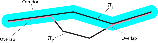
Figure 7: In the proximity penalty computation, the overlap of two paths is determined by drawing a corridor around the path, $\pi_{j}$, then measuring the part of the path $\pi_{j^{\prime}}$ that lies within that corridor.

• $\mathscr{C}_{B}(\pi_{j})$ is the base travel cost as computed by the search in the $H_{2}$-augmented graph (i.e. estimated time taken to follow the path without consideration for any other agent in the environment).

• The second term computes the additional cost due to the a priori belief of traffic density, $\rho$, modeled to be proportional to the net estimated traffic density along the path, $\mathscr{C}_{T}(\pi_{j})=\sum_{s\in\pi_{j}}\rho(s)$ – referred to as the traffic-weighted travel cost, and scaled by the estimated number of distant agents, $Q$, in the environment. The proportionality constant, $a$, is determined experimentally (described in the next paragraph).

• The last term computes the proximity penalty or overlap cost between pairs of paths due to multiple contending robots from different (or the same) paths creating congestion along the regions of $\pi_{j}$ where there is a geometric overlap with $\pi_{j^{\prime}}$ (Figure 7). This includes self-overlap cost (when $j^{\prime}=j$) due to the multiplicity of contending robots following the $j$-th path. The cost is proportional${}^{\ref{foot:lin}}$ to the number of additional contending robots, $N_{j^{\prime}}(\sigma)$, in the overlapping path and the amount of overlap, $\mathscr{C}_{P}(\pi_{j},\pi_{j^{\prime}})$. The amount of overlap itself consists of two parts: $\mathscr{C}_{P}(\pi_{j},\pi_{j^{\prime}})=\mathscr{C}_{P,B}(\pi_{j},\pi_{j^{\prime}})+a\,Q\,\mathscr{C}_{P,T}(\pi_{j},\pi_{j^{\prime}})$, where the first part is the time cost of the part of the path $\pi_{j^{\prime}}$ that overlaps with $\pi_{j}$ as is computed by the search in the $H_{2}$-augmnted graph (with the overlap being determined by the proximity between the points on the two paths – Figure 7), and $\mathscr{C}_{O,T}(\pi_{j},\pi_{j^{\prime}})$ is the net estimated traffic density on the overlapping parts of $\pi_{j^{\prime}}$.

The values of $a$ and $b$ are determined experimentally by running multiple simulations in a simple single-passage map (Figure 8) with a varying number of distant agents (we choose pedestrians only) and a varying number of contending robots. The width and the length of the passage in this map are chosen to be similar to those in the maps used in experiments and simulations. For more details on the implementation of the simulations, refer to Section 4.

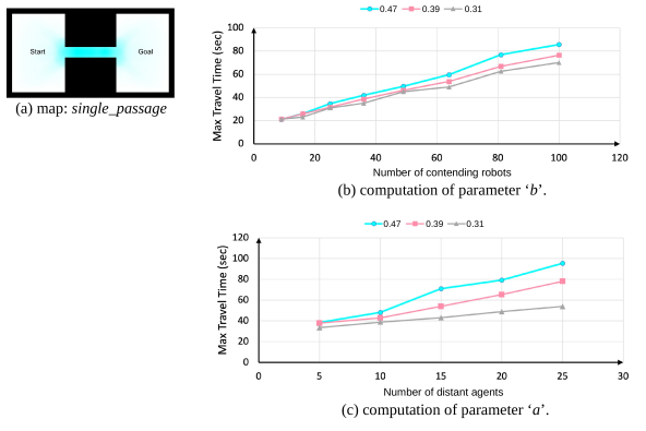
Figure 8: Experimental estimation of the proportionality constants $a$ and $b$ in (2). The curves in different colors in (b) and (c) are with different ratios of the robot’s safety distance to the passage’s width as that is different for different environments. (a) The single-passage map used to experimentally compute the proportionality constants $a$ and $b$, with the estimated traffic density, $\rho$ colored in cyan. (b) Max travel time increases with the number of contending robots, with the fixed number of pedestrians. The slope of this curve computes the constant $b$. (c) Max travel time increases with the number of pedestrians, with the number of robots fixed at 10. The slope of this curve computes the constant $a$.

3.5 Simplified Formulations

The optimization problem in (1) is referred to as the complete model and has $O(m^{n})$ terms in the objective function, making it extremely computationally expensive to solve with a large number of robots and available topological classes. We thus propose couple of approximations to simplify the optimization problem. These approximations rely on the fact that the number of contending robots, $n$, that the planning robot assumes is an estimate and is purely for the purpose of computing its own path choice probabilities. In reality, there is no coordination or communication between nearby robots. We thus use extreme values of $n$ to simplify the models.

3.5.1 Two-robot Model

In this model we assume that the number of contending robots the planning robot considers is $n=2$, so that the objective function in (1) becomes quadratic, which can be solved efficiently using a quadratic program. However, in computing the travel time cost for the $j$-th path, $D_{j}(\sigma)$, with $\sigma\in S^{2}$, we can still account for a number $n$ other than $2$ by simply replacing each of the $2$ robots with $\frac{n}{2}$ robots when computing the overlap costs. This is effectively done in (2) by scaling & redefining the robot counting function as $N_{j^{\prime}}(\sigma)=\frac{n}{2}|R_{j^{\prime}}(\sigma)|,\leavevmode\nobreak\ \sigma\in S^{2}$.

3.5.2 Ensemble Model

In this model the planning robot assumes a large number of contending robots so that the number of robots in the $j$-th class is approximately $nP_{j}$. Considering the problem of minimizing the maximum travel time cost (i.e., the maximum out of the travel times of all the contending robots) This allows us to reformulate the optimization problem as

$$\min_{P_{1},P_{2},\cdots,P_{m}}\Big{(}\max_{j\in S}\leavevmode\nobreak\ K_{j}(P_{1},P_{2},\dots,P_{m})\Big{)}$$ (3)

s.t. $$\sum_{j=1}^{m}P_{j}=1\leavevmode\nobreak\ ,\quad 0\leq P_{j}\leq 1,\leavevmode\nobreak\ \forall j\in S$$

where $K_{j}(P_{1},P_{2},\dots,P_{m})$ is the estimated travel time cost for a robot assigned to the $j$-th path if the number of robots following the $l$-th path is $nP_{l}$ for all $l\in S$. The expression of $K_{j}$ is derived naturally from the definition of $D_{j}$ in (2):

$$\!\!\!\!\!\!\!\!\!\!\!\!K_{j}(P_{1},P_{2},\dots,P_{m})$$

$$=\mathscr{C}_{B}(\pi_{j})+a\,Q\,\mathscr{C}_{T}(\pi_{j})+b\,\sum_{j^{\prime}\in S}\!\mathscr{C}_{P}(\pi_{j},\pi_{j^{\prime}})\leavevmode\nobreak\ nP_{j^{\prime}}$$

$$\approx nb\,\sum_{j^{\prime}\in S}\!\mathscr{C}_{P}(\pi_{j},\pi_{j^{\prime}})P_{j^{\prime}}\quad\text{(since $n$ is large)}$$ (4)

Note that $K_{j}(P_{1},P_{2},\dots,P_{m})$ is affine in $\{P_{j}\}_{l\in S}$, and hence the objective function in (3) being $\max$ of affine functions, is convex (boyd2004convex, ). As a consequence, the optimization problem in (3) can be solved using efficient numerical methods and does not have an exponentially large number of terms as was the case in (1). It is worth noting that there is no meaningful analogous ensemble model for minimization of the average travel time cost since the average of the affine functions, $\{K_{j}\}_{j\in S}$, would result in an affine objective function in (3), which would result in a linear program, the solutions to which is always trivial with one of the probabilities in $\{P_{j}\}_{j\in S}$ being equal to $1$ and rest $0$.

3.5.3 Path Choice Probability Values

Given a planning robot’s start and goal location in an environment, the path choice probabilities, $\{P_{j}\}_{j\in S}$, depend on the choice of the model (complete model, 2-robot model or ensemble model) as well as the number of contending agents, $n$. For the ensemble model, with the large $n$ assumption, it is clear from (3) and (4) that the probability values are independent of the choice of $n$. A comparison of the probability values computed using the different models and different $n$ is shown in Table 1. The similarity among the values computed using the complete model and the $2$-robot model is apparent, while the values from the ensemble model get closer to the $2$-robot model as the value of $n$ increases. This allows us to choose a simplified model for fast computation of the probabilities in experiments and simulations with a large number of contending robots.

Table 1: A comparison of the probability distribution over classes by different models on Map “cage_1” without non-rational agents. The paths of classes are shown in Figure LABEL:pic_classes.

Contd. Rbt. # $n$	Probability Distribution ($m=3$)*
	Class 1	Class 2	Class 3
Complete Model: Average Travel Time Cost
5	0.64071	0.35917	0.00012
10	0.54207	0.35219	0.10574
15	0.49175	0.35085	0.15740
20	—**	—**	—**
Complete Model: Maximum Travel Time Cost
5	0.76014	0.23985	0.00000
10	0.67781	0.32215	0.00004
15	0.54728	0.38163	0.07109
20	—**	—**	—**
$2$-robot Model: Average Travel Time Cost
5	0.70690	0.29310	0.00000
10	0.55048	0.34206	0.10746
15	0.48449	0.33841	0.17710
20	0.45323	0.33669	0.21009
25	0.43499	0.33568	0.22933
30	0.42304	0.33502	0.24194
$2$-robot Model: Maximum Travel Time Cost
5	0.63448	0.36552	0.00000
10	0.46863	0.36812	0.16325
15	0.42046	0.35715	0.22239
20	0.40036	0.35227	0.24737
25	0.38933	0.34950	0.26117
30	0.38237	0.34772	0.26991
Ensemble Model: Maximum Travel Time Cost
Any $n$	0.36570	0.33185	0.30245

• All methods use $a=0.1625$, $b=0.04548$, and $Q=0$.

• Not computable due to the memory overflow in computation of $3^{20}$ terms in the objective function of the complete model.

4 Execution of Chosen Path with Local Collision Avoidance

In this section we describe the algorithm and controller used by a robot for following the stochastically chosen path in a topological class while avoiding immediate collisions based on local sensing.

The overall algorithm for each robot is as follows: A robot stochastically chooses a reference path from the paths $\{\pi_{j}\}_{j\in S}$ that it computed using A* search in the $H_{2}$-augmented graph according to its own computed probability distribution $\{P_{j}\}_{j\in S}$. Once a robot chooses its own reference path, it commits to that path, since without inter-robot coordination and without live global traffic updates, there is not new information to warrant a full-blown replanning of reference path. Each robot then starts executing its reference path while performing a fast replanning (described in Section 4.2) at regular intervals of time with an appropriately chosen heuristic function in order to follow the reference path while avoiding collision with pedestrians and other robots. The fast replanning is performed using A* search in the $H_{2}$-augmented graph, $\mathcal{G}_{H_{2}}$, and does not compute the path choice probabilities, but simply avoids high pedestrian/robot density regions as estimated in the immediate future in the spatio-temporal domain using sensing of the immediate vicinity. Feedback linearization and a potential-based approach allows control of the robot while avoiding collision. The following subsections give more details on prediction of agent density in the immediate spatiotemporal neighborhood (Section 4.1), the fast replanning algorithm (Section 4.2), and a potential-based local collision avoidance for the non-holonomic robot model (Section 4.3).

4.1 Spatio-temporal Representation of Other Agents’ Near-future Occupancy Probability Distribution

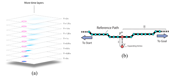
Figure 9: Fast replanning: (a) Illustration of computation of a nearby agent’s probability in X-Y-T configuration space with $\delta_{t}=0.25s$. The lighter cyan, the less likely it is occupied by the agent. The red ring shows the region (including safety radius) occupied by the agent at the time of prediction. (b) Heuristic function for fast re-planning returns the estimated time of travel for the parts I and II.

For each agent in its immediate vicinity, a robot performs a short-term prediction of the agent’s occupancy probability distribution as a density function in its spatio-temporal configuration space. Given the instantaneous position and velocity of a nearby agent (estimated using sensors onboard the robot), the robot employs a simple prediction-only Markov localization approach (FOX1998195, ; zhan2021frontiers, ) (a discrete analog of Kalman filter) that uses a motion model to predict the probability of occupancy distribution (in a uniform discrete representation of the spatio-temporal domain) of the agent for the next $m_{\text{max}}$ timesteps (with each times-step of length $\delta t$, and a spatial discretization of $\delta r^{\prime}$ – the same discretization used in construction of $\mathcal{G}$ – Section 2.3). These occupancy probability values from the different nearby agents are aggregated (point-wise maximum) to construct the probability of occupancy map, $\mathcal{P}(x,y,t)$, that assigns a value to every discrete cell (Figure LABEL:pic_timelayers). In practice, the probability computations are done on-the-fly during the graph search and only for $t$ between the current time and $m_{\text{max}}$ time-steps into the future.

4.2 Fast Replanning – Heuristic Function and Cost Function

In order to perform a fast re-planning to avoid collision with other nearby agents, while ensuring that a robot stays committed to its reference path, we design a reference-path-based heuristic function for guiding an A* search on the $H_{2}$-augmented graph $\mathcal{G}_{H_{2}}$ for quickly computing a path in the same homology class as the reference path. The heuristic function for the fast re-planner for a vertex $(\mathbf{v},t,h)\in\mathcal{V}_{H_{2}}$ is computed as follows (Figure LABEL:pic_heuristic_re-planning): We compute the closest vertex $\mathbf{p}^{*}=\arg\!\min_{\mathbf{p}\in\pi_{\text{ref}}}\|\mathbf{x}-\mathbf{p}\|$ on the reference path, $\pi_{\text{ref}}$ (described as a sequence of points on the planar domain), and return the Euclidean distance between $\mathbf{v}$ and $\mathbf{p}^{*}$ (referred to as part I of the heuristic function), and add to it the cost (travel time) from $\mathbf{p}^{*}$ to the goal on the reference path (referred to as part II of the heuristic function) which was pre-computed as part of the reference path search in $H_{2}$-augmented graph. More formally, the heuristic function evaluated at $(\mathbf{x},t,h)\in\mathcal{V}_{H_{2}}$ is described as $h_{\pi_{\text{ref}}}(\mathbf{x},t,h)=\alpha\left(\frac{\|\mathbf{x}-\mathbf{p}^{*}\|}{V_{\text{max}}}+C_{\pi_{\text{ref}}}(\mathbf{p}^{*})\right)$, where $\alpha\leq 1$ is a constant to tune the inadmisibility of the heuristic function, with lower value of $\alpha$ allowing greater deviation of the re-planned path from the reference path.

The cost function for fast replanning not only tries to minimize travel time, but also accounts for the computed nearby agent probability of occupancy, $\mathcal{P}$. In particular, the cost of an edge, $e\in\mathcal{E}$, connecting two points in the spatio-temporal domain is described by $C_{\mathcal{G}}(e)=\int_{\overline{e}}\frac{1+\iota}{1+\iota-\mathcal{P}(x,y,t)}\,dt$, where the integration is a line integration on the segment representing the edge and is performed numerically using linear interpolation of $\mathcal{P}$ along the uniformly discretized segment, and $\iota=0.001$ is a small positive constant used for numerical stability. Note that if the probability of occupancy is close to $1$ at some point, that point will have very high cost and will hence be avoided.

4.3 Non-holonomic Robot Control for Trajectory Tracking and Potential-based Collision Avoidance

Trajectory tracking: Each robot tracks its computed trajectory (the reference trajectory at the beginning, and the fast-replanned trajectory subsequently). In the experiments, each non-holonomic differential drive robot controls a lookahead point (d1992dynamic, ) by computing the corresponding linear and angular velocities. At a given time step, a target point $\mathbf{p}_{l}=(x_{l},y_{l})$ is extracted from the time parametrized trajectory output by the re-planning algorithm. This set point is tracked using a feedback linearization controller designed as follows: Given the current robot position $\mathbf{p}_{c}=(x_{c},y_{c})$, orientation $\theta_{c}$ and a constant lookahead distance $d_{f}$, a Cartesian velocity $\mathbf{v}=(v_{x},v_{y})=c_{s}(\mathbf{p}_{l}-\mathbf{p}_{d})$ is computed for a point, $\mathbf{p}_{d}=(x_{d},y_{d})=(x_{c}+d_{f}\cos\theta_{c},y_{c}+d_{f}\sin\theta_{c})$, which is a point at a distance $d_{f}$ ahead of the robot. This enables the lookahead point track the target point $\mathbf{p}_{l}$. $c_{s}$ is a constant scalar gain. Corresponding linear and angular velocities for the robot is thus computed as $u=v_{x}\cos\theta_{c}+v_{y}\sin\theta_{c}$ and $\omega=(v_{y}\cos\theta_{c}-v_{x}\sin\theta_{c})/d_{f}$. For the differential drive robot, linear and angular velocities can be mapped to left and right wheel efforts (or velocities) as $v_{L}=u-\omega l/2$ and $v_{R}=u+\omega l/2$ where $l$ is the separation between the two wheels of the robot.

Local collision avoidance with other agents: Depending on the robot heading, a fan-shaped collision cone is generated in front of the robot with radius $r_{c}$ and angle $\alpha_{c}$. For every other agent, $i$, detected inside the collision cone with position $\mathbf{p}_{\text{agnt},i}=(x_{\text{agnt},i},y_{\text{agnt},i})$, a repulsion velocity to slow down the robot, that is inversely proportional to the distance between them, is computed as $\mathbf{v}_{\text{rep},i}=-c_{\text{a}}\,(\mathbf{p}_{\text{agnt},i}-\mathbf{p}_{c})/\|\mathbf{p}_{\text{agnt},i}-\mathbf{p}_{c}\|^{2}$, where $c_{\text{a}}$ is a positive constant. The resulting Cartesian velocity of the robot is computed as $\mathbf{v}_{\text{avoid}}=\mathbf{v}+\sum_{i}\mathbf{v}_{\text{agnt},i}$. This emulates the behavior of a vehicle that tries to avoid other agents ahead of it, but not behind it.

Local collision avoidance with obstacles: For avoiding robot-environment collision (including environment boundaries and obstacles) we use a velocity cancellation policy as follows: The closest point on an obstacle or environment boundary to the robot is denoted as $\mathbf{p}_{\text{env}}=(x_{\text{env}},y_{\text{env}})$. Then the vector from the robot to the environment is defined as $\mathbf{v}_{\text{env}}=\mathbf{p}_{\text{env}}-\mathbf{p}_{c}$. An obstacle repulsion component of the velocity is activated only if the obstacle is sufficiently close, and the robot has a velocity component towards the obstacle, and thus the final velocity of the robot is computed as follows:

$\mathbf{v}_{\text{final}}=\left\{\begin{array}[]{ll}\mathbf{v}_{\text{avoid}}-c_{\text{e}}\,(\mathbf{v}_{\text{avoid}}\cdot\mathbf{v}_{\text{env}})\mathbf{v}_{\text{env}}/\|\mathbf{v}_{\text{env}}\|^{2},&\leavevmode\nobreak\ \leavevmode\nobreak\ \text{if }\|\mathbf{v}_{\text{env}}\|<d_{e}\text{ and }\mathbf{v}\cdot\mathbf{v}_{\text{env}}>0,\\ \mathbf{v}_{\text{avoid}},&\leavevmode\nobreak\ \leavevmode\nobreak\ \text{otherwise.}\end{array}\right.$

where, $c_{\text{e}}$ and $d_{e}$ are positive constants.

5 Results & Discussions

We run the simulations on several maps: “cage_1” (Figure LABEL:pic_classes), “cage_2” (Figure LABEL:pic_density_map_1), “lehigh” (Figure LABEL:pic_density_map_2), “o2” (Figure LABEL:pic_o2), and “group” (Figure LABEL:pic_group). Three types of comparisons are made:

1. We first compare our proposed topological planning algorithm (a robot stochastically choosing paths from available topological classes) with a shortest-path algorithm (each robot, without any inter-robot coordination, chooses the shortest path to goal). In this comparison all distant agents are modeled as pedestrians and their trajectories are randomly generated.

2. Then, we demonstrate the effectiveness of a. the traffic density map, and, b. the proposed computation of path choice probabilities by comparing the performance of our algorithm with versions that either does use an uniform traffic density map or uniformly path choice probabilities over the topological classes.

3. Finally, we apply our proposed method to a setup with multiple groups of robots that start from different locations and have different goal locations, and compare the performance of our method with the performance of the shortest-path algorithm.

It is worth noting that the fundamental premise of lack of inter-agent coordination or communication makes our work extremely unique. We assume that there exists no inter-agent communication or coordination, and robots do not share their plan or intent with other agents or with any central server. No other prior work, to our knowledge, assumes complete lack of communication or coordination (for example, in street2021congestion there exists communication and coordination between the robots in construction of a shared PRT). Hence a fair comparison of our method with such alternatives in literature is not possible.

i. In the topological-versus-shortest-path comparison, the robots are allowed to choose one out of up to $m=6$ classes. In each environment we vary the number of robots, $n$, and the number of pedestrians, $Q$, and note the average travel time of the robots and the maximum travel time (the time taken by the last robot to reach its goal). We also measure the average time spent on collision avoidance per robot. A simulation with the same initial conditions is performed using each of the proposed topological algorithm and the shortest path algorithm. Tables 2 and 3 shows a performance comparison. Each of the percentage numbers is the ratio of travel time (average or maximum) between the simulations using the topological algorithm and that using the shortest path algorithm. For collisions we show the difference between the time spent avoiding collisions using the topological algorithm and that using the shortest path algorithm In computing the path assignment probability values for the topological algorithm we can use either the maximum travel time cost, $C_{\text{max}}$, or the average travel time cost, $C_{\text{avg}}$, and choose one out of the two simplified formulations – 2-robot model (solved using QP library ‘qpOASES’) or the ensemble model (solved using NLP library ‘NLopt’). This is indicated in the first column of the tables.

As evident from the results, as the number of robots and pedestrians increase (i.e., the potential of congestion increases), our proposed topological algorithm significantly outperforms the shortest path algorithm in all aspects. It is also worth noting that in the larger lehigh map, using the travel time costs $C_{\text{max}}$, the advantage is higher in the maximum travel time than the average travel time.

Table 2: Performance of our proposed topological algorithm as compared to a shortest path algorithm in simulations for map “cage_1”, using two time-cost & assignment probability computation models. Darker cyan indicates bigger advantage of the topological algorithm over the shortest-path one, while darker red indicates cases where it underperformed. Each cell shows the the average over 10 simulation runs with different initial conditions. See multimedia attachment for sample simulation runs.

Method	Feature	Ped. #	Robot #
			5	10	15	20
2-robot Model, minimizing Avg. Travel Time Cost	Avg. travel time	0	95.27%	87.67%	80.52%	75.44%
		5	93.78%	86.59%	82.05%	72.41%
		10	94.60%	80.00%	78.87%	71.12%
		15	90.68%	76.95%	66.80%	60.63%
		20	78.51%	104.11%	74.36%	72.50%
		25	94.08%	115.45%	93.12%	72.28%
		30	80.32%	65.95%	56.22%	54.44%
	Max. travel time	0	90.72%	80.78%	73.41%	67.27%
		5	90.60%	82.18%	75.30%	69.17%
		10	90.19%	70.53%	74.91%	70.06%
		15	83.84%	73.83%	61.88%	58.50%
		20	77.07%	111.23%	76.51%	71.93%
		25	98.84%	128.70%	96.81%	70.97%
		30	82.64%	63.98%	48.89%	53.23%
	Collision (s)	0	-0.01	-0.05	-0.35	-0.49
		5	-0.03	-0.13	-0.88	-1.63
		10	-0.05	-0.10	-1.22	-1.54
		15	-0.08	-0.27	-1.57	-2.55
		20	-0.21	-3.92	-3.41	-5.17
		25	-0.20	-4.86	-4.95	-5.41
		30	-0.34	-0.17	-1.24	-2.84
Ensemble Model, minimizing Max. Travel Time Cost	Avg. travel time	0	111.56%	90.25%	82.04%	75.55%
		5	115.29%	90.41%	79.99%	71.99%
		10	108.19%	83.36%	82.94%	69.79%
		15	99.85%	74.00%	70.07%	62.32%
		20	89.91%	98.68%	72.78%	69.40%
		25	94.89%	109.67%	87.84%	74.45%
		30	82.13%	66.33%	59.58%	55.01%
	Max. travel time	0	109.48%	83.52%	73.95%	66.68%
		5	112.16%	85.17%	74.40%	64.25%
		10	100.58%	75.71%	85.01%	65.39%
		15	89.90%	69.52%	64.88%	61.92%
		20	96.68%	105.01%	75.10%	68.03%
		25	98.23%	124.14%	87.29%	72.70%
		30	82.95%	61.12%	52.84%	52.27%
	Collision (s)	0	-0.01	-0.05	-0.31	-0.34
		5	-0.04	-0.08	-1.01	-1.50
		10	-0.05	-0.15	-1.13	-1.42
		15	-0.10	-0.33	-1.46	-2.02
		20	-0.19	-3.89	-3.30	-4.62
		25	-0.21	-4.91	-5.11	-5.67
		30	-0.30	-0.45	-1.00	-3.60

• All methods use $a=0.1625$, $b=0.04548$.

• % values: $\frac{\text{time taken in topological algorithm}}{\text{time taken in shortest path algorithm}}\times 100\%$

• Collision numbers: (colliding duration per robot in topological algorithm) - (colliding duration per robot in shortest-path algorithm)

Table 3: Performance comparisons in the other two maps.

Method	Feature	Ped. #	Robot #
			5	10	15	20
Map: cage_2
$2$-robot Model, Avg. Time Cost	Avg (%)	0	95.85%	90.29%	84.85%	80.81%
		5	86.65%	79.37%	76.02%	68.26%
		10	85.97%	69.49%	70.12%	61.40%
		15	75.84%	73.91%	58.37%	57.25%
		20	76.86%	61.80%	51.63%	51.70%
	Max (%)	0	93.18%	85.70%	78.55%	74.66%
		5	86.11%	79.69%	69.92%	64.10%
		10	84.49%	66.14%	69.57%	62.41%
		15	80.55%	76.35%	57.79%	50.84%
		20	76.73%	58.49%	53.16%	50.63%
	Collision (s)	0	-0.04	-0.05	0.23	0.41
		5	-0.02	-0.13	-0.05	0.48
		10	-0.01	-0.13	0.27	-0.28
		15	-0.18	-0.23	-0.02	-4.58
		20	-0.18	0.21	-2.20	-6.96

Map: lehigh
Method	Feature	Ped. #	10	20	30	40	50
Ensemble Model, Max. Time Cost	Avg (%)	0	104.20%	97.99%	91.13%	91.27%	91.77%
		20	101.19%	93.67%	91.53%	83.36%	81.93%
		40	98.09%	97.74%	89.98%	84.98%	80.06%
		60	95.61%	91.20%	82.21%	77.04%	72.55%
		80	119.92%	92.39%	80.57%	73.80%	70.18%
		100	99.30%	85.08%	75.62%	72.94%	71.27%
	Max (%)	0	110.32%	95.62%	85.99%	85.78%	88.53%
		20	106.89%	95.49%	89.06%	80.53%	80.11%
		40	105.61%	105.41%	89.96%	81.80%	76.91%
		60	98.76%	89.79%	76.87%	69.52%	66.96%
		80	132.74%	89.90%	72.13%	66.38%	60.62%
		100	99.15%	84.85%	68.58%	67.18%	60.94%
	Collision (s)	0	0.00	0.02	0.00	-0.01	-3.04
		20	0.00	0.00	-0.55	-0.02	-0.02
		40	0.00	-0.30	0.25	-0.05	-0.05
		60	0.00	-0.02	-0.01	-0.09	-0.09
		80	-1.38	0.01	-0.09	0.06	-0.89
		100	-0.01	0.04	-0.14	-0.45	-1.72

ii. a. To verify that the traffic density map (as described in Section 3.2) in our proposed algorithm makes a difference in performance, we used a uniform traffic density map to run 10 simulations for comparison (while keeping the rest of the algorithm the same). The results in Table 4 suggests that the algorithm without an appropriately computed traffic density map underperforms. The role of the traffic density map in predicting the traffic for computation of the path assignment probabilities is statistically significant.

ii. b. To demonstrate the effectiveness of our proposed path assignment probability computation, we compare the performance of our ensemble model for probability computation with uniform path assignment probabilities. In particular, in map o2 (Figure LABEL:pic_o2), the ensemble model minimizing the max. travel time cost gives path assignment probabilities of $0.34$, $0.25$, $0.26$ and $0.14$ for the $4$ topological classes in the environment, which is sufficiently different from uniform probability of $0.25$ for all the classes. This makes this environment a prime candidate for comparison of our method with the uniform path assignment probability method. Table 5 shows that the path assignment probabilities computed using the proposed algorithm leads to an improved performance with a variety of robot and pedestrian setups, when compared against the uniform path assignment probability method.

Table 4: Performance comparisons between simulations using traffic density map, $\rho$, and not using it (i.e., effectively uniform traffic density by setting traffic density term 0) on Map “cage_1”, both with 6 classes, 10 robots, 10 pedestrians, and using the 2-robot model minimizing average travel time cost. Each cell shows the the average over 10 simulation runs with different initial conditions.

Using TDM (s)		Not Using TDM (s)		Comparison (%)
Avg	Max	Avg	Max	Avg	Max
62.14	124.83	67.14	143.45	92.57%	87.02%

Table 5: Performance comparisons between simulations using path assignment probabilities computed using the ensemble model minimizing max. travel time cost, and using an uniform path assignment probability over 4 topological classes on map “o2” (Figure LABEL:pic_o2). Each cell shows the the average over 10 simulation runs with different initial conditions.

Robot #	Ped. #	Ensemble Model (s)		Uniform Path Assignment (s)		Comparison (%)
		Avg	Max	Avg	Max	Avg	Max
5	5	43.01	61.81	49.61	72.94	86.70%	84.74%
10	10	75.66	142.06	91.16	150.30	82.99%	94.51%
15	15	106.53	196.84	120.04	237.92	88.74%	82.73%

Table 6: Performance comparisons for multi-group scenarios (3 groups, 5 robots in each group) between the topological method and the shortest-path method in map “group” (Figure LABEL:pic_group). The topological method uses ensemble model minimizing max. time time cost with 10 classes. Each cell shows the the average over 10 simulation runs with different initial conditions.

Topological (s)		Shortest (s)		Comparison (%)
Avg	Max	Avg	Max	Avg	Max
59.7901	107.439	65.0912	115.988	91.86%	92.63%

iii. Although most of our simulations focus on single-group scenarios, we have applied our algorithm to a multi-group case as well. In map “group” (Figure LABEL:pic_group), three groups of robots starting of from different locations try to reach their respective goals cross the map. As suggested by Table 6, our method, with 10 classes for robots to choose from performs better than the shortest-path algorithm in a statistically significant manner.

Real Robot Experiments: Real-robot experiments were run only on the cage_2 map with 9 robots and 9 pedestrians (Fig 10). The results from each of the 10 runs are summarized in Table 7 and demonstrate similar advantages as seen in simulations. Complete video of the simulation can be found in the multimedia attachment. It is to be noted that the robots used in the experiments are omni-directional and are is allowed to stop and/or move back in order to avoid immediate collision with other robots or pedestrians that it can sense in its immediate neighborhood. Since the robots follow paths computed by A* planer on a discrete grid representation of the environment, it needs to follow a piece-wise path that is restricted to the graph.

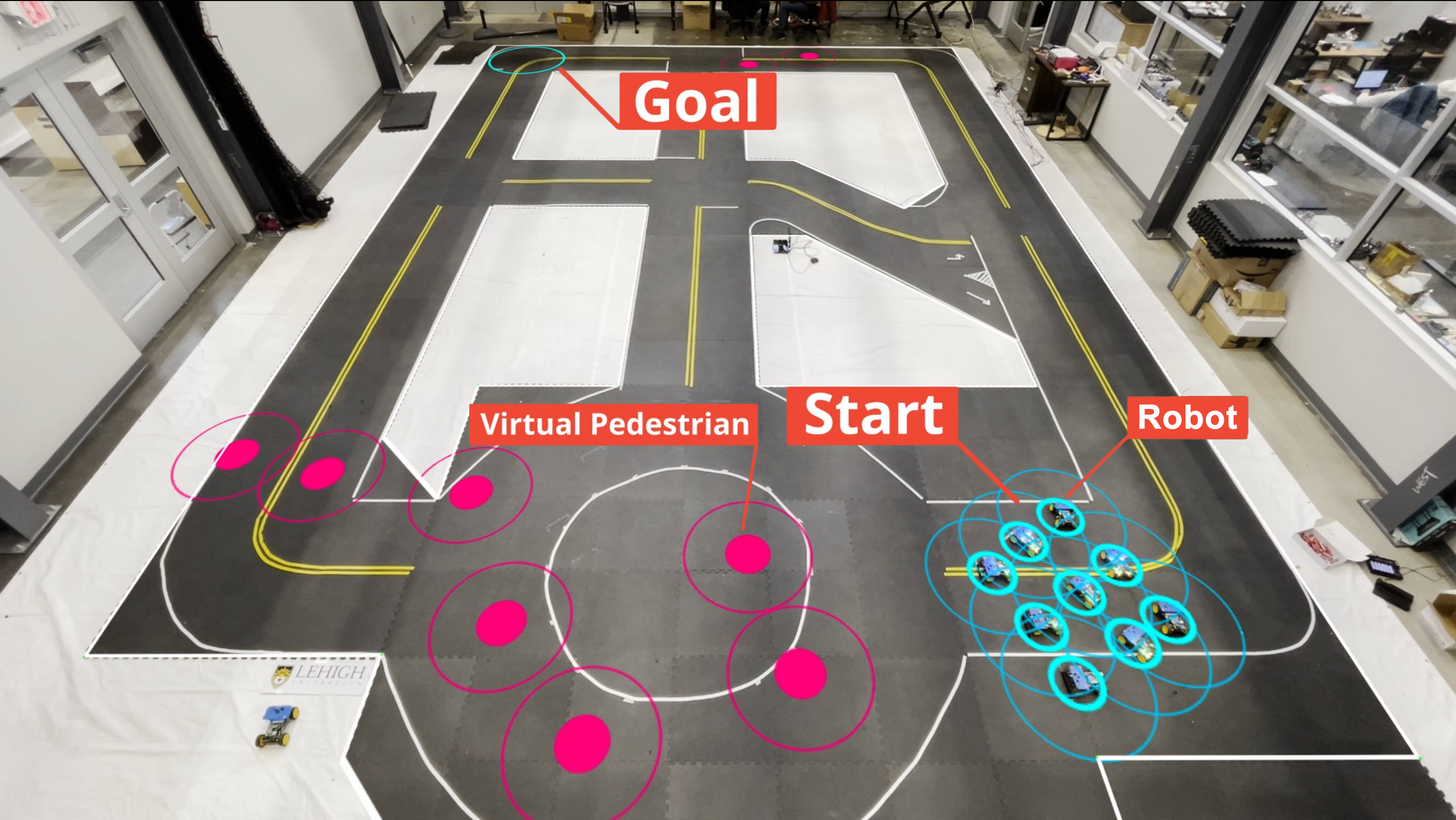
Figure 10: Real robot experiment in map “cage_2”. Virtual (augmented reality) pedestrians are used in the experiment (see multimedia attachment).

Table 7: Statistic from individual real-robot experiments on map “cage_2”. All runs are with 9 robots and 9 virtual pedestrians, using the 2-robot model minimizing average travel time cost, $C_{\text{avg}}$.

	Topological (s)			Shortest (s)			Avg	Max	Coll
Expt.#	Avg	Max	Coll	Avg	Max	Coll	(ratio)	(ratio)	(diff.)
1	56.82	86.20	0.00	86.93	143.14	0.02	65.37%	60.22%	-0.02
2	70.04	120.27	0.20	72.76	116.96	0.19	96.26%	102.83%	0.01
3*	76.32	94.45	0.17	111.68	162.72	0.70	68.34%	58.04%	-0.53
4	60.69	116.82	0.00	106.08	138.78	0.68	57.21%	84.18%	-0.68
5	57.32	85.92	0.04	79.75	96.77	0.37	71.87%	88.79%	-0.32
6	57.69	99.05	0.43	98.10	201.87	0.44	58.81%	49.07%	-0.01
7	46.83	55.03	0.34	90.86	132.60	0.61	51.55%	41.50%	-0.27
8	51.59	82.63	0.07	83.15	105.48	0.43	62.04%	78.34%	-0.37
9	63.45	81.31	0.20	86.74	129.86	0.54	73.15%	62.61%	-0.34
10	65.42	140.28	0.29	130.53	169.16	0.67	50.12%	82.92%	-0.38
						Avg	65.47%	70.85%	-0.29

• See this run in the supplementary video.

• All experiments use $a=0.0001$, $b=0.7222$.

Discussions, Limitations and Future Directions: As demonstrated in the simulations and the experiments, our inter-agent coordination-free method distributing the agents across different routes outperforms other coordination-free methods with respect to the overall travel time. The advantage is particularly amplified when there are a large number of robots in the environment. Compared to other MAPF methods, our method does not require real-time traffic information of both in- and out-of-system agents. The probability computation time using one of the simplified models for each robot is constant irrespective of the number of agents in the environment, and hence the computation complexity per robot does not increase with the number of agents, making our algorithm suitable for an environment with a large number of agents.

Despite the demonstrated effectiveness of the proposed method, we recognize several limitations of the current method, which warrant further future investigations:

1. We use a priory traffic density estimation in the cost function for computing the reference paths for each robot. Currently this traffic density is computed synthetically purely based on the structure/map of the environment. In a real urban environment, historic traffic date can provide more accurate traffic density. In future we plan to test the proposed method with real traffic data collected from the department of transportation for constructing the traffic density map.

2. It is assumed that each robot has a priori knowledge of the environment (a map) and also knows its own location (using a global localization system such as GPS). Without one or both of these information, each robot will also need to simultaneously create a map of the environment and/or localize itself in the environment. This will require each robot to use a SLAM (Simultaneous Localization and Mapping) jia2019survey module on top of our coordination-free planning algorithm, which we will do in the future.

3. We have used A* search algorithm in a discrete graph representation of the environment for computing the cost-minimizing paths restricted to the graph. This results in the individual robots following paths that are piecewise linear, but may have sudden turns because of the discrete nature of the graph. In future we will use any-angle planning algorithms such Theta* daniel2010theta or S* bhattacharya2019towards to generate smoother paths for the individual robots to follow.

Acknowledgments

This material is based upon work supported by the National Science Foundation under Grant No. CCF-2144246.

References

- \bibcommenthead
- (1) Silver, D.: Cooperative pathfinding. In: Proceedings of the Aaai Conference on Artificial Intelligence and Interactive Digital Entertainment, vol. 1, pp. 117–122 (2005)
- (2) Sharon, G., Stern, R., Felner, A., Sturtevant, N.R.: Conflict-based search for optimal multi-agent pathfinding. Artificial Intelligence 219, 40–66 (2015)
- (3) Han, S.D., Yu, J.: Ddm: Fast near-optimal multi-robot path planning using diversified-path and optimal sub-problem solution database heuristics. IEEE Robotics and Automation Letters 5(2), 1350–1357 (2020)
- (4) Wagner, G., Choset, H.: M*: A complete multirobot path planning algorithm with performance bounds. In: Intelligent Robots and Systems (IROS), 2011 IEEE/RSJ International Conference On, pp. 3260–3267 (2011). IEEE
- (5) Mohanan, M.G., Salgoankar, A.: A survey of robotic motion planning in dynamic environments. Robotics and Autonomous Systems 100, 171–185 (2018). https://doi.org/10.1016/j.robot.2017.10.011
- (6) Kushleyev, A., Likhachev, M.: Time-bounded lattice for efficient planning in dynamic environments. In: 2009 IEEE International Conference on Robotics and Automation, pp. 1662–1668 (2009)
- (7) Cai, K., Wang, C., Cheng, J., De Silva, C.W., Meng, M.Q.-H.: Mobile robot path planning in dynamic environments: A survey. arXiv e-prints, 2006–14195 (2020) arXiv:2006.14195 [cs.RO]
- (8) Hasan, A.H., Mosa, A.M.: Multi-robot path planning based on max–min ant colony optimization and d* algorithms in a dynamic environment. In: 2018 International Conference on Advanced Science and Engineering (ICOASE), pp. 110–115 (2018)
- (9) Ziebart, B.D., Ratliff, N., Gallagher, G., Mertz, C., Peterson, K., Bagnell, J.A., Hebert, M., Dey, A.K., Srinivasa, S.: Planning-based prediction for pedestrians. In: 2009 IEEE/RSJ International Conference on Intelligent Robots and Systems, pp. 3931–3936 (2009). IEEE
- (10) Kretzschmar, H., Spies, M., Sprunk, C., Burgard, W.: Socially compliant mobile robot navigation via inverse reinforcement learning. The International Journal of Robotics Research 35(11), 1289–1307 (2016)
- (11) Kirby, R., Simmons, R., Forlizzi, J.: Companion: A constraint-optimizing method for person-acceptable navigation. In: RO-MAN 2009-The 18th IEEE International Symposium on Robot and Human Interactive Communication, pp. 607–612 (2009). IEEE
- (12) Sisbot, E.A., Marin-Urias, L.F., Alami, R., Simeon, T.: A human aware mobile robot motion planner. IEEE Transactions on Robotics 23(5), 874–883 (2007)
- (13) Ferrer, G., Garrell, A., Sanfeliu, A.: Social-aware robot navigation in urban environments. In: 2013 European Conference on Mobile Robots, pp. 331–336 (2013). IEEE
- (14) Shiomi, M., Zanlungo, F., Hayashi, K., Kanda, T.: Towards a socially acceptable collision avoidance for a mobile robot navigating among pedestrians using a pedestrian model. International Journal of Social Robotics 6(3), 443–455 (2014)
- (15) Atzmon, D., Stern, R., Felner, A., Sturtevant, N.R., Koenig, S.: Probabilistic robust multi-agent path finding. In: Proceedings of the International Conference on Automated Planning and Scheduling, vol. 30, pp. 29–37 (2020)
- (16) Santos, V.G., Chaimowicz, L.: Hierarchical congestion control for robotic swarms. In: 2011 IEEE/RSJ International Conference on Intelligent Robots and Systems, pp. 4372–4377 (2011). IEEE
- (17) Toutouh, J., Alba, E.: A swarm algorithm for collaborative traffic in vehicular networks. Vehicular Comms. 12, 127–137 (2018)
- (18) Antoniou, P., Pitsillides, A., Blackwell, T., Engelbrecht, A., Michael, L.: Congestion control in wireless sensor networks based on bird flocking behavior. Computer Networks 57(5), 1167–1191 (2013). https://doi.org/10.1016/j.comnet.2012.12.008
- (19) Tatomir, B., Rothkrantz, L.: Hierarchical routing in traffic using swarm-intelligence. In: 2006 IEEE Intelligent Transportation Systems Conference, pp. 230–235 (2006). https://doi.org/10.1109/ITSC.2006.1706747
- (20) Gunes, M., Sorges, U., Bouazizi, I.: Ara-the ant-colony based routing algorithm for manets. In: Proceedings. International Conference on Parallel Processing Workshop, pp. 79–85 (2002). IEEE
- (21) Di Caro, G., Ducatelle, F., Gambardella, L.M.: Anthocnet: an adaptive nature-inspired algorithm for routing in mobile ad hoc networks. European Transactions on Telecommunications 16(5), 443–455 (2005)
- (22) Street, C., Pütz, S., Mühlig, M., Hawes, N., Lacerda, B.: Congestion-aware policy synthesis for multirobot systems. IEEE Transactions on Robotics (2021)
- (23) Stump, E., Michael, N.: Multi-robot persistent surveillance planning as a vehicle routing problem. In: IEEE International Conference on Automation Science and Engineering, pp. 569–575 (2011)
- (24) Leahy, K., Zhou, D., Vasile, C.-I., Oikonomopoulos, K., Schwager, M., Belta, C.: Persistent surveillance for unmanned aerial vehicles subject to charging and temporal logic constraints. Auton. Robots 40(8), 1363–1378 (2016). https://doi.org/10.1007/s10514-015-9519-z
- (25) Kusnur, T., Mukherjee, S., Saxena, D.M., Fukami, T., Koyama, T., Salzman, O., Likhachev, M.: A Planning Framework for Persistent, Multi-UAV Coverage with Global Deconfliction. In: Proceedings of the 12th Conference on Field and Service Robotics (2019)
- (26) Thakur, D., Likhachev, M., Keller, J., Kumar, V., Dobrokhodov, V., Jones, K., Wurz, J., Kaminer, I.: Planning for Opportunistic Surveillance with Multiple Robots. In: IEEE/RSJ International Conference on Intelligent Robots and Systems (2013)
- (27) Van den Berg, J., Lin, M., Manocha, D.: Reciprocal velocity obstacles for real-time multi-agent navigation. In: 2008 IEEE International Conference on Robotics and Automation, pp. 1928–1935 (2008). Ieee
- (28) Mavrogiannis, C.I., Knepper, R.A.: Multi-agent path topology in support of socially competent navigation planning. The International Journal of Robotics Research 38(2-3), 338–356 (2019)
- (29) Mavrogiannis, C., Balasubramanian, K., Poddar, S., Gandra, A., Srinivasa, S.S.: Winding through: Crowd navigation via topological invariance. IEEE Robotics and Automation Letters 8(1), 121–128 (2022)
- (30) LaValle, S.M.: Robot motion planning: A game-theoretic foundation. Algorithmica 26(3), 430–465 (2000)
- (31) He, C., Wan, Y., Gu, Y., Lewis, F.L.: Integral reinforcement learning-based multi-robot minimum time-energy path planning subject to collision avoidance and unknown environmental disturbances. IEEE Control Systems Letters 5(3), 983–988 (2020)
- (32) Bhattacharya, S., Likhachev, M., Kumar, V.: Topological constraints in search-based robot path planning. Autonomous Robots, 1–18 (2012). DOI: 10.1007/s10514-012-9304-1
- (33) Bhattacharya, S., Ghrist, R.: Path homotopy invariants and their application to optimal trajectory planning. Annals of Mathematics and Artificial Intelligence 84(3-4), 139–160 (2018)
- (34) Wang, X., Bhattacharya, S.: A topological approach to workspace and motion planning for a cable-controlled robot in cluttered environments. IEEE Robotics and Automation Letters 3(3), 2600–2607 (2018). https://doi.org/10.1109/LRA.2018.2817684
- (35) Govindarajan, V., Bhattacharya, S., Kumar, V.: Human-robot collaborative topological exploration for search & rescue applications. In: Intl. Symp. on Distributed Autonomous Robotic Sysystems (2014)
- (36) Bhattacharya, S., Ghrist, R., Kumar, V.: Persistent homology for path planning in uncertain environments. IEEE Transactions on Robotics (T-RO) 31(3), 578–590 (2015)
- (37) Wu, W., Bhattacharya, S., Prorok, A.: Multi-robot path deconfliction through prioritization by path prospects. In: Proceedings of IEEE Intl. Conference on Robotics and Automation (ICRA) (2020)
- (38) Bhattacharya, S., Kim, S., Heidarsson, H., Sukhatme, G., Kumar, V.: A topological approach to using cables to separate and manipulate sets of objects. International Journal of Robotics Research 34(6), 799–815 (2015). DOI: 10.1177/0278364914562236
- (39) Choset, H., Lynch, K.M., Hutchinson, S., Kantor, G.A., Burgard, W., Kavraki, L.E., Thrun, S.: Principles of Robot Motion: Theory, Algorithms, and Implementations. Principles of Robot Motion: Theory, Algorithms, and Implementations. MIT Press, Cambridge, MA (2005)
- (40) Boyd, S., Vandenberghe, L.: Convex Optimization. Cambridge university press, Cambridge, UK (2004)
- (41) Fox, D., Burgard, W., Thrun, S.: Active markov localization for mobile robots. Robotics and Autonomous Systems 25(3), 195–207 (1998). Autonomous Mobile Robots
- (42) Zhang, L., Prorok, A., Bhattacharya, S.: Pursuer assignment and control strategies in multi-agent pursuit-evasion under uncertainties. Frontiers in Robotics and AI 8, 262 (2021). https://doi.org/10.3389/frobt.2021.691637
- (43) d’Andrea-Novel, B., Bastin, G., Campion, G.: Dynamic feedback linearization of nonholonomic wheeled mobile robots. In: Proceedings 1992 IEEE International Conference on Robotics and Automation, pp. 2527–2528 (1992). IEEE Computer Society
- (44) Jia, Y., Yan, X., Xu, Y.: A survey of simultaneous localization and mapping for robot. In: 2019 IEEE 4th Advanced Information Technology, Electronic and Automation Control Conference (IAEAC), vol. 1, pp. 857–861 (2019). IEEE
- (45) Daniel, K., Nash, A., Koenig, S., Felner, A.: Theta*: Any-angle path planning on grids. Journal of Artificial Intelligence Research 39, 533–579 (2010)
- (46) Bhattacharya, S.: Towards optimal path computation in a simplicial complex. The International Journal of Robotics Research 38(8), 981–1009 (2019)