Coherent enhancement of optical remission in diffusive media
From the earth’s crust to the human brain, remitted waves are used for sensing and imaging in a diverse range of diffusive media. Separating the source and detector increases the penetration depth of remitted light, yet rapidly decreases the signal strength, leading to a poor signal-to-noise ratio. Here, we experimentally and numerically show that wavefront shaping a laser beam incident on a diffusive sample enables an order of magnitude remission enhancement, with a penetration depth of up to 10 transport mean free paths. We develop a theoretical model which predicts the maximal-remission enhancement. Our analysis reveals a significant improvement in the sensitivity of remitted waves, to local changes of absorption deep inside diffusive media. This work illustrates the potential of coherent wavefront control for non-invasive diffuse-wave imaging applications, such as diffuse optical tomography and functional near-infrared spectroscopy.
Introduction
The remission geometry is broadly used for imaging and sensing deep inside random media (?, ?, ?, ?, ?, ?, ?, ?, ?), because it combines the non-invasiveness of reflection with the deep-penetration of transmission. In real world applications where transmitted waves are either inaccessible or strongly attenuated, diffusive waves remitted from the same side of the medium as their source are collected as signals (?, ?). To enhance the penetration depth of detected signals, the source and detector are spatially separated on the medium’s surface. With increasing source-detector distance , waves from the source migrate deeper into the diffusive medium before reaching the detector (?, ?). Their paths are distributed over a banana-shaped region with two ends connecting the source and the detector, with the mid-region reaching deepest (close to ). Since the waves generated by the source diffuse in all directions, only a small portion eventually reaches the detector. The signal strength decays rapidly with increasing the source-detector separation; thus the signal-to-noise ratio (SNR) is poor for large penetration depths.
Recent advances in optical wavefront shaping have enabled the control of coherent wave transport in random scattering media, enhancing light transmission and energy deposition (?, ?). Finding the optimal wavefront for an incident beam mostly relies on the detector/camera on the other side or a guide star inside the medium (?, ?). Non-invasive focusing and imaging schemes have been developed utilizing: the optical memory effect (?, ?, ?, ?), nonlinear excitation (?, ?), the interaction between light and acoustic waves (?, ?, ?, ?, ?, ?), and linear fluorescence (?, ?, ?, ?). Moreover, steady-state and time-gated reflection eigenchannels are employed for focusing light onto –and image reconstruction of– embedded targets (?, ?, ?, ?). In these setups the backscattered signals, which are collected at the same location as the injected light, have a penetration depth less than or comparable to the transport mean free path (?, ?). Spatial displacement of a source and a detector –the common geometry for diffuse optical tomography (DOT) and functional near-infrared spectroscopy (fNIRS)– has yet to be explored in wavefront shaping experiments; even though remitted waves can go much deeper than into a diffusive sample (?, ?).
Here we shape the incident wavefront of a monochromatic laser beam to enhance remitted waves at source-detector distances . The key issue is whether the penetration depth is compromised by remission enhancement. We demonstrate, experimentally and numerically, an order of magnitude enhancement of remission with no change in the penetration depth up to 10 deep. Our theoretical model predicts the maximal-remission enhancement and its dependence on the source-detector separation , the transport mean free path , and the number of input and output channels. Finally we analyze the sensitivity of remitted waves, to local changes of absorption deep inside diffusive media. The maximum remission eigenchannel enhances the sensitivity by one order of magnitude. This work illustrates the power of wavefront shaping for steering coherent waves deep inside diffusive media, with potential applications in DOT and fNIRS.
Experimental Setup
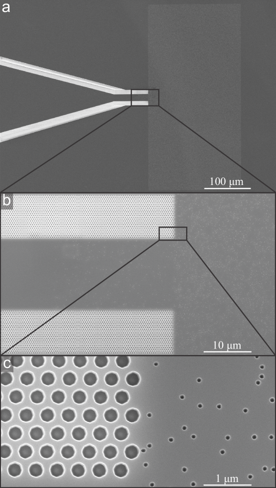
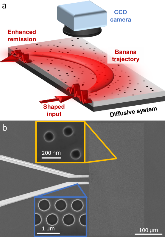
In order to monitor the migration paths of remitted waves inside the diffusive medium, we fabricate two-dimensional (2D) disordered structures on a silicon chip and observe the internal light distribution from the third dimension [Fig. 1 (a)] (?). The remission matrix is introduced to relate input fields within a finite region of the interface to remitted waves from another region displaced from the injection site, on the same interface. We experimentally measure for different separations from 3 to 25, find the maximum-remission eigenstates, and investigate their spatial structures.
The 2D diffusive system has a slab geometry (width = 400 µm, thickness = 200 µm) and open boundaries on all four sides [Fig. 1(b)]. Inside the slab, air holes of 100 nm diameter are randomly distributed with a filling fraction of . The transport mean free path is µm at (vacuum) wavelength µm (?). With slab dimensions and much larger than but still smaller than the 2D localization length, light transport is diffusive. Out-of-plane scattering is treated as loss, corresponding to a diffusive dissipation length of = 56 µm (see supplementary section 1.1).
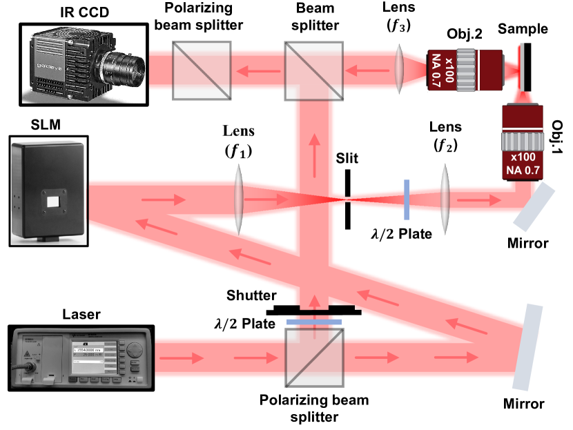
A spatial light modulator (SLM) shapes the phase front of the monochromatic laser beam, which is then coupled into a multimode waveguide etched on a silicon-on-insulator wafer. The waveguide delivers light of 1.55 µm to a 2D slab on the same chip via 56 guided modes. The field distribution across the entire slab is measured in an interferometric setup. We scan the input wavelength to obtain different configurations.
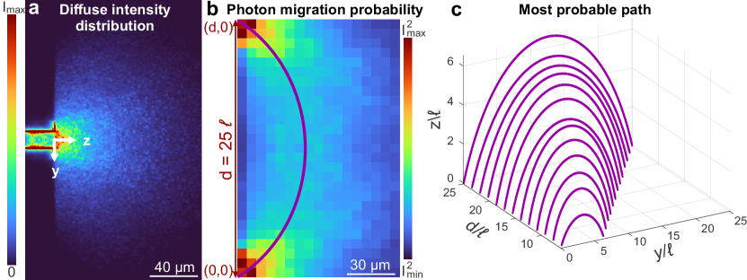
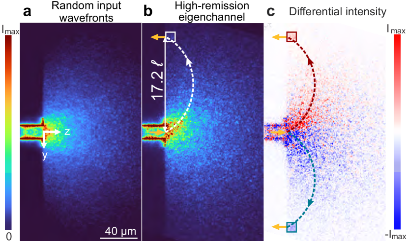
First, we generate random illumination patterns using the SLM, and map diffusive light transport inside the slab. Figure 2(a) shows the ensemble-averaged intensity distribution . The injection site is centered at and has a width = 15 µm. Away from it, the intensity of the remitted light drops quickly. Along the front boundary of the slab, the diffusive intensity decreases quadratically with distance .
The probability of photon migration from the injection site to the remission site via the position inside the slab equals the product of the probability of migrating from to and that from to . The former is proportional to , and the latter to the average intensity distribution for light injected at , according to optical reciprocity (?). With random incident wavefronts, the maximum probability of photon migration follows a banana-shaped trajectory from to . While increasing injection-remission separation gives access to deeper-penetrating light, it comes at the price of a rapidly reduced signal strength.
Remission Matrix & Eigenchannels
Our aim is to utilize the spatial degrees of freedom in the coherent illumination pattern to improve the remitted signal strength. To find the optimal input wavefront, we measure the remission matrix , and find its associated eigenstates. In a standard DOT setup, light is delivered onto a diffusive sample by a waveguide and the remitted signal is collected by another waveguide. The incident field and remitted field are decomposed into and flux-carrying modes of the waveguides. In a linear scattering medium, they are related by the remission matrix as
| (1) |
Singular value decomposition of gives the remission eigenchannels. The one corresponding to the largest singular value has the highest possible remittance.
While the waveguide mode basis is used in Eq. 1, any orthogonal basis is sufficient. In our experiment, instead of using a waveguide to collect the remitted light, we directly measure the field at the front boundary of the slab at a distance from the injection waveguide. More specifically, we sample the fields at spatial positions within a 10 µm 10 µm square. By displaying orthogonal phase patterns on the SLM, we construct the remission matrix . Singular value decomposition of provides the remission eigenchannels and associated input vectors. Since our SLM can only modulate phase, not amplitude, it will not excite a pure eigenchannel. Alternatively, we measure the matrix that connects the incoming fields to the field everywhere inside the slab. Multiplying it by the input vector of a remission eigenchannel recovers the field distribution across the entire slab.
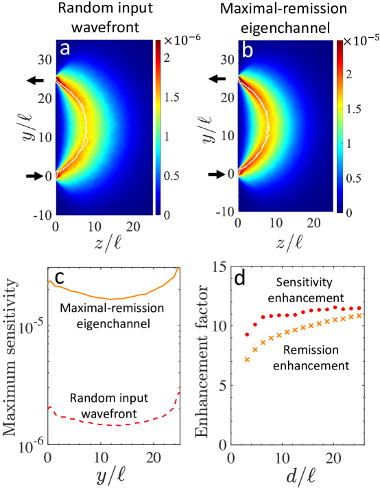
Figure 2(b) shows an example high-remission eigenchannel profile . The remission region (white square) is located at from the input waveguide. shows that the diffuse light is steered towards the detector via the banana trajectory, which is obtained by tracing the maximum photon migration probability under random illumination (see supplementary section 1.3). The steering is further illustrated by the difference in Fig. 2(c). The positive (red) or negative (blue) intensity pattern reveals light is directed towards the remission site at or . In both cases, high-remission eigenchannels redistribute optical energy along the banana trajectories connecting the injection and detection sites.
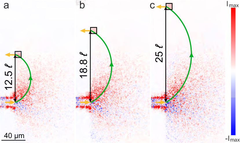
We vary the injection-detection distance and plot the difference between high-remission eigenchannel profile and random input pattern for , in Fig. 3. The positive (red) and negative (blue) intensity areas demonstrate that high-remission eigenchannels redistribute optical energy inside the system compared to random inputs. Furthermore, the positive (red) intensity regions in (a-c) concentrate along the banana trajectories (green line). Therefore, it is possible to direct the flow of light deep inside diffusive systems by coupling into high-remission eigenchannels. The penetration depth is not affected at all by the remission enhancement.
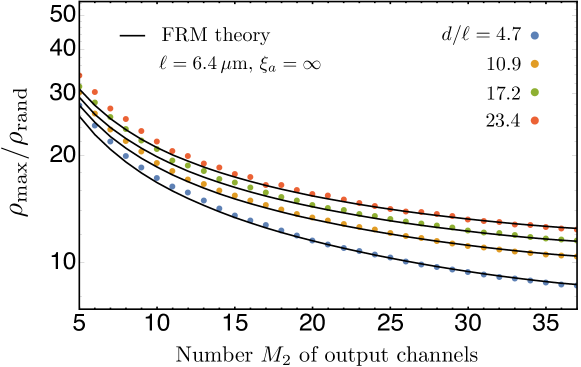
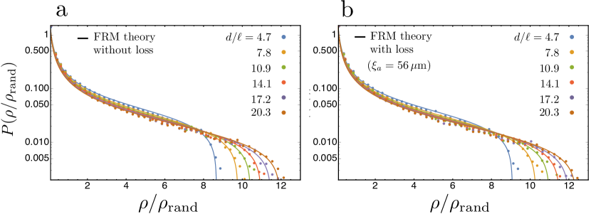
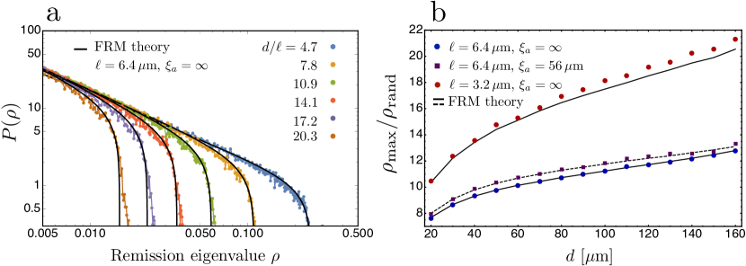
In our experiment, wavefront shaping can also increase the out-of-plane scattering from the detection site, which inflates the remission intensity. We thus resort to numerical simulations of the experimental system to quantify the remission enhancement as a function of . For this purpose, we simulate wave propagation in 2D disordered slabs using the Kwant package (?, ?), and compute the remission matrix with input channels and output channels. The eigenvalues of give the fraction of power remitted to the output waveguide of width µm when sending the associated input vectors into the slab. We represent in Fig. 4(a) the probability density function (PDF) of non-zero eigenvalues, , for a broad range of source-detector distance (larger than the transport mean free path µm). The PDF decays monotonically, indicating that most eigenstates deliver little power at the remission port. However, we note that the PDF presents an upper edge much larger than (the fraction of power delivered by random input illumination). For example, of the total injected power can be remitted at a distance , compared to for random illumination. As the distance increases, all eigenvalues get smaller, since less power is collected, and the PDF narrows. To quantify the benefit of using the eigenstate associated with the largest remission eigenvalue instead of random illumination, we represent in Fig. 4(b) the ratio as a function of the distance . Enhancement typically larger than is reached (blue circles). Remarkably, the enhancement increases with , which illustrates the power of coherent wavefront control for . When including out-of-plane scattering loss in our simulations (purples squares), the enhancement slightly increases because dissipation has more impact on the random input propagation than on a high-remission eigenchannel (?); see supplementary section 2.4 for the full distributions in the presence of loss. Moreover, increasing the scattering strength of the disordered medium through a reduction of (red triangles) leads to further enhancement of remission , which can be as large as at µm.
To elucidate the intricate dependence of and on relevant parameters , , , and , we develop a theoretical model based on a combination of random matrix theory and microscopic computations of intensity fluctuations in remission. Our approach relies on the concept that any structure consisting of effective diffusive systems with comparable conductance in series is characterized by a universal bimodal eigenvalue distribution, irrespective of the microscopic origin of scattering and the geometry of the scattering system (?). This distribution, initially put forward for transmission through diffusive wires (?), can in principle be used for the remission configuration, as long as input and output spatial channels do not belong to the same waveguide. However in our setup, light propagates in an open geometry with input/output covering only a small fraction of the total surface area. Therefore, we must also take into account the incomplete channel control of the injection and detection. We model the remission matrix as a filtered matrix of dimension , drawn from a virtual matrix characterized by a bimodal distribution of eigenvalues with mean , and use the predictions of the filtered random matrix (FRM) ensemble (?). The only free parameters of this model are thus and , which can be determined from microscopic calculations of the first two moments of the distribution . Details of the full model are given in supplementary section 2. Solid lines in Fig. 4(a,b) show our theoretical predictions for and its upper edge , which are in excellent agreement with the numerical results.
Next we consider limiting cases. If the number of output spatial channels is equal to 1, the remission enhancement equals the number of input channels , regardless of the injection-remission distance and the transport mean free path . As increases, the maximal remitted signal grows, but the enhancement drops. A key quantity controlling the scaling of with microscopic parameters is the non-Gaussian component of intensity fluctuations measured at the remission port and generated by random illumination from the injection port. These fluctuations are commonly termed (?); see supplementary section 2.2 for their explicit calculation. When is small, , the remission matrix can be approximated by a Gaussian random matrix, and the enhancement factor scales as (?, ?, ?). However, if is larger, , non-Gaussian intensity correlations can further enhance the remission. In a 2D diffusive system, leads to the increase of with both scattering strength and injection-remission distance . Indeed, in the situation we find that the remission enhancement depends on a single parameter: the normalized variance of the PDF , related to as , where (see supplementary section 2.2). In the limit , the remission enhancement takes the form (supplementary section 2.3)
| (2) |
Contrary to the remission under random illumination , the high-remission eigenchannel generates a flux that is independent of the scattering strength . Ignoring the weak dependence of on , the enhancement factor scales linearly with the number of input channels . Furthermore, the dependence of on and explains the general trends beyond the above limits in Fig. 4(b). We refer to the supplementary section 4.3 for a study of the continuous evolution of with .
Sensitivity Analysis
Given that high-remission eigenchannels improve the signal-to-noise ratio, a natural question is whether they provide higher sensitivity to local perturbations of the dielectric constant inside a diffusive medium. The answer is important to DOT and fNIRS, which often monitor the change in remitted signal due to localized absorptive targets. The answer to this question is not straightforward because sensitivity depends not only on the value of remission, but also on position inside the medium, as shown below. Furthermore, prior analysis of the problem, based on the diffusion equation (?), is not applicable as the enhanced remission here is achieved through wave interference: which is not captured by diffusion theory.
Let be the total power collected at the remission port divided by the incident power for an arbitrary incident field . With fixed, a small amount of absorption is introduced as the imaginary part of the relative permittivity over a subwavelength area centered at location . It changes the collected remission by . The sensitivity is defined as . Under the scalar wave equation approximation in 2D, we show in supplementary section 3 that
| (3) |
where is the vacuum wave number, is the total field given as the incident field, and is the total field with in the remission port as the incident field. Eq. (3) generalizes the adjoint method commonly used in inverse designs (?) to multi-channel systems. We evaluate the sensitivity for different input wavefront in our numerical simulation.
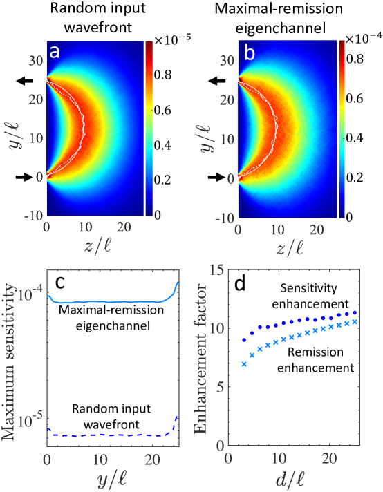
Figure 5(a-b) shows the ensemble-averaged sensitivity map computed using Eq. (3) for random input wavefronts and for high-remission eigenchannels respectively, in a lossless system. The sensitivity map of high-remission eigenchannels has the same spatial profile as that of random inputs, with the sensitivity maximized along the banana trajectory. The high-remission eigenchannels improve the sensitivity about 11 times along such trajectory in Fig. 5(c). We further find that the sensitivity enhancement increases with , similar to the remission enhancement. Notably, the sensitivity enhancement is even larger than the remission enhancement in Fig. 5(d). To illustrate that the sensitivity depends not just on the remission, we separate the incident and the scattered contributions of the conjugate field, . The numerator of Eq. (3) has two terms: and . A high-remission eigenchannel naturally enhances the first term which is proportional to the remission for near the remission port, but it may also increase the second term to further enhance the sensitivity. Similar results are observed in systems with loss (Supplementary Fig. 12).
Discussion & Conclusion
We have shown that coherent wavefront shaping greatly enhances the remitted signal and its sensitivity to local change of absorption deep inside a diffusive medium. Our method differs from the existing method of structured illumination in optical tomography, which utilizes an incoherent light and modulates only its intensity (?). While the latter improves the speed and accuracy of image reconstruction, it does not increase the remitted signal (?, ?). In our case, coherent light must be used for illumination, both its amplitude and phase are modulated. The phase modulation is essential to the enhancement of remitted signal via constructive interference of multiply scattered light.
While the current study is conducted on 2D diffusive systems, our method is applicable to 3D, so is our theoretical model. The remission enhancement increases with , but decreases with . A difference from 2D is that the maximal-remission enhancement in 3D no longer varies with , because becomes independent of (supplementary section 2.3). However, the dependence due to is preserved. In DOT and fNIRS, the commonly used 3D biological samples have negligible , and the maximal-remission enhancement is approximately , according to the Marcenko–Pastur law (?).
In conclusion, we have introduced and investigated, both theoretically and experimentally, the concept of remission eigenchannels in open diffusive systems with a slab geometry. Using our on-chip interferometric platform, we measure remission matrices and investigate the associated eigenchannel profiles inside disordered systems. Selective excitation of high-remission eigenchannels significantly enhances the signal strength of diffusive remitted light with deep penetration up to 10 transport mean free paths. The greatly improved sensitivity of remitted signals, to local perturbations deep inside diffusive media, is promising for many diffusive-wave imaging and sensing applications, ranging from seismology to noninvasive photomedical devices and brain-computer interfaces.
References
- 1. A. Yodh, B. Chance, Spectroscopy and imaging with diffusing light, Phys. Today 48, 34 (1995).
- 2. M. Campillo, A. Paul, Long-range correlations in the diffuse seismic coda, Science 299, 547 (2003).
- 3. A. P. Gibson, J. C. Hebden, S. R. Arridge, Recent advances in diffuse optical imaging, Phys. Med. Biol. 50, R1 (2005).
- 4. T. Durduran, R. Choe, W. B. Baker, A. G. Yodh, Diffuse optics for tissue monitoring and tomography, Rep. Prog. Phys. 73, 076701 (2010).
- 5. A. T. Eggebrecht, et al., Mapping distributed brain function and networks with diffuse optical tomography, Nat. Photon. 8, 448 (2014).
- 6. J. Gunther, S. Andersson-Engels, Review of current methods of acousto-optical tomography for biomedical applications, Front. Optoelectron. 10, 211 (2017).
- 7. M. A. Yücel, J. J. Selb, T. J. Huppert, M. A. Franceschini, D. A. Boas, Functional near infrared spectroscopy: enabling routine functional brain imaging, Curr. Opin. Biomed. Eng. 4, 78 (2017).
- 8. J. P. Angelo, et al., Review of structured light in diffuse optical imaging, J. Biomed. Opt. 24, 071602 (2018).
- 9. K. Wapenaar, J. Brackenhoff, J. Thorbecke, Green’s theorem in seismic imaging across the scales, Solid Earth 10, 517 (2019).
- 10. D. A. Boas, et al., Imaging the body with diffuse optical tomography, IEEE Signal Process. Mag. 18, 57 (2001).
- 11. M. Ferrari, V. Quaresima, A brief review on the history of human functional near-infrared spectroscopy (fNIRS) development and fields of application, Neuroimage 63, 921 (2012).
- 12. W. Cui, C. Kumar, B. Chance, Time-Resolved Spectroscopy and Imaging of Tissues (International Society for Optics and Photonics, 1991), vol. 1431, pp. 180–191.
- 13. S. Feng, F.-A. Zeng, B. Chance, Photon migration in the presence of a single defect: a perturbation analysis, Appl. Opt. 34, 3826 (1995).
- 14. A. P. Mosk, A. Lagendijk, G. Lerosey, M. Fink, Controlling waves in space and time for imaging and focusing in complex media, Nat. Photon. 6, 283 (2012).
- 15. S. Rotter, S. Gigan, Light fields in complex media: mesoscopic scattering meets wave control, Rev. Mod. Phys. 89, 015005 (2017).
- 16. R. Horstmeyer, H. Ruan, C. Yang, Guidestar-assisted wavefront-shaping methods for focusing light into biological tissue, Nat. Photon. 9, 563 (2015).
- 17. S. Yoon, et al., Deep optical imaging within complex scattering media, Nat. Rev. Phys. 2, 141 (2020).
- 18. J. Bertolotti, et al., Non-invasive imaging through opaque scattering layers, Nature 491, 232 (2012).
- 19. O. Katz, P. Heidmann, M. Fink, S. Gigan, Non-invasive single-shot imaging through scattering layers and around corners via speckle correlations, Nat. Photon. 8, 784 (2014).
- 20. H. Yılmaz, et al., Speckle correlation resolution enhancement of wide-field fluorescence imaging, Optica 2, 424 (2015).
- 21. G. Stern, O. Katz, Noninvasive focusing through scattering layers using speckle correlations, Opt. Lett. 44, 143 (2019).
- 22. J. Tang, R. N. Germain, M. Cui, Superpenetration optical microscopy by iterative multiphoton adaptive compensation technique, Proc. Natl. Acad. Sci. U.S.A. 109, 8434 (2012).
- 23. O. Katz, E. Small, Y. Guan, Y. Silberberg, Noninvasive nonlinear focusing and imaging through strongly scattering turbid layers, Optica 1, 170 (2014).
- 24. X. Xu, H. Liu, L. V. Wang, Time-reversed ultrasonically encoded optical focusing into scattering media, Nat. Photon. 5, 154 (2011).
- 25. B. Judkewitz, Y. M. Wang, R. Horstmeyer, A. Mathy, C. Yang, Speckle-scale focusing in the diffusive regime with time reversal of variance-encoded light (TROVE), Nat. Photon. 7, 300 (2013).
- 26. T. Chaigne, et al., Controlling light in scattering media non-invasively using the photoacoustic transmission matrix, Nat. Photon. 8, 58 (2014).
- 27. C. Ma, X. Xu, Y. Liu, L. V. Wang, Time-reversed adapted-perturbation (TRAP) optical focusing onto dynamic objects inside scattering media, Nat. Photon. 8, 931 (2014).
- 28. P. Lai, L. Wang, J. W. Tay, L. V. Wang, Photoacoustically guided wavefront shaping for enhanced optical focusing in scattering media, Nat. Photon. 9, 126 (2015).
- 29. O. Katz, F. Ramaz, S. Gigan, M. Fink, Controlling light in complex media beyond the acoustic diffraction-limit using the acousto-optic transmission matrix, Nat. Commun. 10, 1 (2019).
- 30. A. Daniel, D. Oron, Y. Silberberg, Light focusing through scattering media via linear fluorescence variance maximization, and its application for fluorescence imaging, Opt. Express 27, 21778 (2019).
- 31. A. Boniface, B. Blochet, J. Dong, S. Gigan, Noninvasive light focusing in scattering media using speckle variance optimization, Optica 6, 1381 (2019).
- 32. A. Boniface, J. Dong, S. Gigan, Non-invasive focusing and imaging in scattering media with a fluorescence-based transmission matrix, Nat. Commun. 11, 1 (2020).
- 33. D. Li, S. K. Sahoo, H. Q. Lam, D. Wang, C. Dang, Non-invasive optical focusing inside strongly scattering media with linear fluorescence, Appl. Phys. Lett. 116, 241104 (2020).
- 34. S. M. Popoff, et al., Exploiting the time-reversal operator for adaptive optics, selective focusing, and scattering pattern analysis, Phys. Rev. Lett. 107, 263901 (2011).
- 35. Y. Choi, et al., Measurement of the time-resolved reflection matrix for enhancing light energy delivery into a scattering medium, Phys. Rev. Lett. 111, 243901 (2013).
- 36. A. Badon, et al., Smart optical coherence tomography for ultra-deep imaging through highly scattering media, Sci. Adv. 2, e1600370 (2016).
- 37. S. Jeong, et al., Focusing of light energy inside a scattering medium by controlling the time-gated multiple light scattering, Nat. Photon. 12, 277 (2018).
- 38. A. Badon, et al., Distortion matrix concept for deep optical imaging in scattering media, Sci. Adv. 6, eaay7170 (2020).
- 39. N. Bender, et al., Depth-targeted energy delivery deep inside scattering media, Nat. Phys. 18, 309 (2022).
- 40. N. Bender, A. Yamilov, H. Yılmaz, H. Cao, Fluctuations and correlations of transmission eigenchannels in diffusive media, Phys. Rev. Lett. 125, 165901 (2020).
- 41. C. W. Groth, M. Wimmer, A. R. Akhmerov, X. Waintal, Kwant: A software package for quantum transport, New J. Phys. 16 (2014).
- 42. R. Sarma, A. Yamilov, S. Petrenko, Y. Bromberg, H. Cao, Control of energy density inside a disordered medium by coupling to open or closed channels, Phys. Rev. Lett. 117 (2016).
- 43. S. F. Liew, S. M. Popoff, A. P. Mosk, W. L. Vos, H. Cao, Transmission channels for light in absorbing random media: from diffusive to ballistic-like transport, Phys. Rev. B 89, 224202 (2014).
- 44. Y. V. Nazarov, Y. M. Blanter, Quantum Transport: Introduction to Nanoscience (Cambridge Univ. Press, 2009).
- 45. C. W. Beenakker, Random-matrix theory of quantum transport, Rev. Mod. Phys. 69, 731 (1997).
- 46. A. Goetschy, A. D. Stone, Filtering random matrices: the effect of incomplete channel control in multiple scattering, Phys. Rev. Lett. 111, 063901 (2013).
- 47. S. Feng, C. Kane, P. A. Lee, A. D. Stone, Correlations and fluctuations of coherent wave transmission through disordered media, Phys. Rev. Lett. 61, 834 (1988).
- 48. S. M. Popoff, A. Goetschy, S. F. Liew, A. D. Stone, H. Cao, Coherent control of total transmission of light through disordered media, Phys. Rev. Lett. 112, 133903 (2014).
- 49. C. W. Hsu, S. F. Liew, A. Goetschy, H. Cao, A. D. Stone, Correlation-enhanced control of wave focusing in disordered media, Nat. Phys. 13, 497 (2017).
- 50. S. Molesky, et al., Inverse design in nanophotonics, Nat. Photon. 12, 659 (2018).
- 51. V. Lukic, V. A. Markel, J. C. Schotland, Optical tomography with structured illumination, Opt. Lett. 34, 983 (2009).
- 52. S. D. Konecky, et al., Quantitative optical tomography of sub-surface heterogeneities using spatially modulated structured light, Opt. Express 17, 14780 (2009).
- 53. R. Pnini, B. Shapiro, Fluctuations in transmission of waves through disordered slabs, Phys. Rev. B 39, 6986 (1989).
Acknowledgments
H.C. and A.Y. thank Michael A. Choma for stimulating discussions. Funding: This work is supported partly by the Office of Naval Research (ONR) under Grant No. N00014-20-1-2197, by the National Science Foundation under Grant Nos. DMR-1905465, DMR-1905442, OAC-1919789, and ECCS-2146021, and by LABEX WIFI (Laboratory of Excellence within the French Program “Investments for the Future”) under references ANR-10-LABX-24 and ANR-10-IDEX-0001-02 PSL*.
Author contributions: N.B. conducted the experiments and analyzed the data; A.Y. performed the numerical simulations and derived the long-range correlations with P.J.P. A.G. developed the analytical model. C.W.H. did the sensitivity analysis with A.G. and A.Y. H.Y. contributed to the experimental study. H.C. initiated the project and supervised the research. All authors contributed to the manuscript writing and editing.
Competing interests: The authors declare no competing financial interests.
Data and materials availability: All data needed to evaluate the conclusions in the paper are present in the paper or the supplementary materials.
Supplementary materials
1 Experiment
1.1 Diffusive Samples
To directly observe the spatial structure of remission eigenchannels inside open diffusive systems, we fabricate two-dimensional diffusive structures on a silicon-on-insulator (SOI) wafer using electron beam lithography and reactive ion etching. An example of the fabricated structure is shown in Fig. 6. The on-chip optical structures we use to route light into the diffusive slab are described in the following paragraphs.
The probe light is injected from the side/edge of the wafer into a ridge waveguide (width = 300 µm, length = 15 mm). It then enters a tapered waveguide (tapering angle = ), shown in Fig. 6(a). The tapered waveguide width decreases gradually from 300 µm to 15 µm. The tapering results in waveguide mode mixing. To avoid significant light leakage, the sidewalls of the tapered waveguide consist of a trigonal lattice of air holes (radius = 155 nm, lattice constant = 440 nm). They provide a 2D complete bandgap for TE polarized light (electric field parallel to the sample surface) within the wavelength range of 1120 nm to 1580 nm. In addition, we etch a 10 µm trench on the outside interface of the photonic crystal layer. The trench scatters light out of the wafer, preventing any light leaking through the photonic-crystal layer from reaching the open diffusive slab. Because the remitted light can be orders of magnitude weaker than the incident light, mitigating any stray light from the input is essential.
As can be seen in Fig. 6(b), we include a “buffer” region in the injection waveguide, after the taper segment, consisting of a small number of random holes (?). The buffer region causes mode mixing in the lead waveguide, ensuring the incident light is distributed over all available spatial channels.
We inject light into a diffusive system configured in a slab geometry with a width of = 400 µm, a depth of = 200 µm, and open boundaries on all sides. Inside the diffusive slab, air holes (diameter = 100 nm) induce light scattering and are randomly distributed with a minimum (edge-to-edge) distance of 50 nm, shown in Fig. 6(c). The filling fraction of air holes is and as a result, the transport mean free path µm and diffusive dissipation length = 56 µm (?). In-plane light scattering by a subwavelength air hole is isotropic, and therefore the transport mean free path is equal to the scattering mean free path.
1.2 Experimental Setup
A detailed schematic of our experimental setup is presented in Fig. 7. A wavelength tunable laser (Keysight 81960A) outputs a linearly-polarized continuous-wave (CW) beam with a wavelength around 1554 nm. The collimated beam is split with a polarizing beam splitter into two beams. One is used as a reference beam –with its polarization subsequently flipped with a half-wave plate– while the other illuminates a phase-only SLM (Hamamatsu LCoS X10468). A one-dimensional (1D) phase-modulation pattern consisting of 128 macropixels is displayed on the SLM. Each macropixel has SLM pixels. We image the field reflected from the SLM plane onto the back focal plane of a long-working-distance objective Obj. 1 (Mitutoyo M Plan APO NIR HR100, Numerical Aperture = 0.7) using two lenses with focal lengths of mm and mm. To prevent the unmodulated light from entering the objective lens, we display a binary diffraction grating within each macropixel to shift the modulated light away from the unmodulated light in the focal plane of the first lens . With a slit in the focal plane, we block all light except the phase-modulated light in the first diffraction order. Right after the slit and before the second lens , we insert a half-wave plate to rotate the polarization of light so that it is transverse-electric (TE) polarized relative to our sample (electric field parallel to the sample surface). The waveguide entrance at the edge of our SOI wafer is placed at the front focal plane of Obj. 1, so that it is illuminated with the Fourier transform of the phase-modulation pattern displayed on the SLM. From the top of the wafer, another long-working-distance objective Obj. 2 (Mitutoyo M Plan APO NIR HR100) collects light scattered out-of-plane from the sample. We use a third lens with a focal length of mm together with Obj. 2 to image the light distribution inside the sample. In conjunction, the lens and the objective magnify the sample image by times. Using a second beam splitter, we combine the signal from the sample with the reference beam. Afterwards, a polarizing beam splitter ensures that the signal has the same polarization as the reference beam. The resulting interference patterns produced by the reference and signal are recorded with an IR CCD camera (Allied Vision Goldeye G-032 Cool).
1.3 Remitted Light For Random Illumination
When a finite region of the disordered slab’s front interface is illuminated with a random wavefront, the light diffuses inside the slab in every direction. The experimentally measured, ensemble-averaged intensity distribution, , generated by random illumination patterns is shown in Fig. 8(a). The intensity distribution for light injected at is obtained by shifting along -axis by a distance . The product is proportional to the probability of photon migrating from the injection site to the remission site via the position inside the diffusive system, as shown in Fig. 8(b). For every cross-section of between and , we locate the maximum probability, max, and fit the corresponding location to part of a circle (purple line) to obtain the most-probable trajectory of the remitted light, for a given injection-remission separation . In Fig. 8(c) we plot such trajectory as a function of . The penetration depth of the remitted light increases with . In order for photons to reach the remission site further away from the injection site, they must travel deeper inside the diffusive system to avoid leaking through the front interface (). While increased injection-remission distance gives access to a larger penetration depth, it comes with the price of a reducion of signal-strength: . Our goal is to use coherent wavefront shaping to manipulate the spatial degrees of freedom, in the incident wavefront, to improve the remitted signal strength without compromising the penetration depth.
1.4 Remission Matrix Measurement
With the interferometric setup shown in Fig. 7, we can determine the field distribution across the disordered region of the sample for any incident wavefront. To measure the field of the light scattered out-of-plane from the sample, for a specific phase modulation pattern displayed on the SLM, we first measure the 2D intensity pattern of the out-of-plane scattered light across the entire disordered region by blocking the reference beam with a shutter. Then after unblocking the reference beam, we retrieve the phase profile of the out-of-plane scattered light with a four-phase measurement. In this measurement, the global phase of the pattern displayed on the SLM is modulated four times in increments of rad. By performing this measurement for a complete, orthogonal set of SLM phase patterns, we reconstruct a linear matrix that maps the field profile on the SLM to the field distribution across the entire slab. The remission matrix is a part of that maps the fields from the SLM to the remission region.
Using , we can recover the spatial field distribution anywhere inside the diffusive slab for any phase modulation pattern on the SLM. To check the accuracy of this recovery, we measure the spatial intensity distribution inside the slab and compare to that given by . The measured spatial intensity distributions of a high-remission eigenchannel generated with phase-only modulation on the SLM have a Pearson correlation coefficient of with the corresponding intensity distribution predicted by .
To experimentally generate different statistical ensembles, we average measurements of the same disorder configuration over different wavelengths of input light from a tunable laser. Specifically, 12 different wavelengths, in increments of 1 nm, from 1547 nm to 1558 nm are averaged to generate our experimental ensembles.
2 Theoretical model and prediction
2.1 Filtered random matrix model
As explained in the main text, the remission matrix is modeled as a filtered random matrix drawn from a larger matrix that characterizes transmission through an arbitrary disordered system supporting input and output propagating channels. This model captures the idea that only a fraction of the scattering channels are effectively excited and detected at the injection and remission sites. Both and the mean of the bimodal eigenvalue PDF of are effective parameters of the model, which are unknown a priori. A theoretical calculation of the flux and its fluctuations detected in the output port will be used to express and in terms of the parameters involved in the remission experiment: the mean free path , the injection-remission distance , and the numbers of input and output spatial channels and .
The mathematical relation between the PDFs of and has been established in Ref. (?). In our remission experiment , so that has non-zero eigenvalues. The PDF of these non-zero eigenvalues, , is equal to the eigenvalue PDF of . According to Ref. (?), it is given by , where is the solution of the equation
| (4) |
where , and
| (5) |
Equation (4) expresses a relation between the Stieltjes transforms and , from which it is possible to express the moments of in terms of those of the eigenvalue PDF of . For the two first cumulants of , we find (?)
| (6) | ||||
| (7) |
We now solve these equations to express the unknown parameters , , and of Eq. (4) in terms of the two first moments and . We get
| (8) | ||||
| (9) | ||||
| (10) |
where . By solving Eq. (4) with above expressions for , , and , we are able to predict the full distribution from the first two moments and only. Figure 4(a) of the main text has been obtained using this procedure. In addition, the upper edge of the PDF is given by (?)
| (11) |
where is the solution of
| (12) |
Theoretical predictions shown in Figure 4(b) of the main text have been generated by evaluating Eq. (11) for different injection-remission distances and mean free paths .
2.2 Theoretical evaluation of and
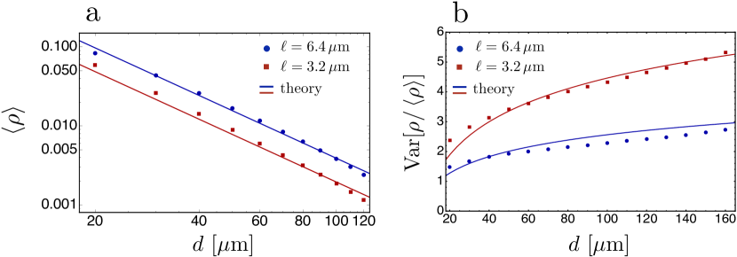
Let us now evaluate analytically the first two moments and of the PDF . First, we note that , where is the mean diffusive flux measured in the output waveguide, also equal to the mean of the eigenvalues of . It is given by
| (13) |
where is the solution of the stationary diffusion equation
| (14) |
In previous equations, is the width of the output waveguide, is the diffusion coefficient of light and is the depth at which the diffusion process is initiated (of the order of the mean free path ). The solution takes the form in the limit . Substituting , we get and
| (15) |
This prediction is compared to numerical simulations in Fig. 9(a).
To find the expression of the normalized variance , we first express it in terms of the full set of eigenvalues (including zeros) of as
| (16) |
Note that . Then, we relate to the fluctuations of the total intensity measured in the output waveguide after exciting a channel of the input waveguide. This is done by means of the singular value decomposition , where is the diagonal matrix . Using this representation, we find . As a result, the fluctuations of depend on the fluctuations of as well as the statistical properties of the matrix . Assuming that is randomly distributed in the unitary group as in Ref. (?), we get
| (17) |
in the limit . The average in the unitary group makes the result independent of the channel . It is thus also equal to the fluctuations of intensity in the output waveguide resulting from a uniform excitation of all modes in the input waveguide. We evaluate the latter by decomposing the field as a sum of all possible scattering contributions reaching the output waveguide. Using standard diagrammatic techniques, we find
| (18) |
with
| (19) |
where is the mean intensity generated inside the disordered material at the position by a uniform illumination of the input waveguide located at the origin, and is the Green’s function of the stationary diffusion equation , evaluated at the position of the output waveguide. The Green’s function being equal to zero at the sample interface, it takes the form
| (20) |
In the limit , the calculation of the integral defining gives
| (21) |
with . The value of is sensitive to regularization procedure required to compute Eq. (19) and, therefore, may deviate in simulations from the value quoted above, while still remaining on the order of unity. Kwant numerical simulation of gives . Finally, the combination of Eq. (16), Eq. (17), and Eq. (18) yields
| (22) |
Numerical simulations of the eigenvalue variance shown in Fig. 9(b) confirm the theoretical result Eq. (22), which predicts a linear dependence on the mean free path as well as logarithmic dependence on the injection-remission distance .
2.3 Approximate FRM solution
In order to gain some insight into the FRM predictions, we can perform an analytical expansion of the exact implicit solution given by Eq. (4). First, we note that for the distance covered in the experiment, the predicted PDF is almost independent of the parameter appearing in Eq. (8) and Eq. (9). Hence, we can take in these equations. We note that still depends on and through and . In addition, we also observe that for µm, which allows us to search for an approximate solution in the limit . In this limit we establish in Ref. (?) that the upper edge of takes the form
| (23) |
where . Using Eq. (8) and Eq. (10) with , we get
| (24) | ||||
| (25) |
For the values of the mean free path and injection-remission distance in our simulation and experiment ( µm or µm, and µm), the parameter takes values . This indicates that the qualitative behavior of can be captured by considering the limit of Eq. (23):
| (26) |
In particular, in the limit , this result predicts that the relative enhancement with respect to the random illumination should scale as
| (27) |
This prediction captures the strong impact of the number of input channels and the mean free path, as well as the weak logarithmic dependence on the distance , observed both in simulations and with the exact FRM solution (see Fig. 4b of the main text). We also note that the leading order given by Eq. (27) is independent of in the limit of large number of remitted channels (). As is progressively increased, the enhancement factor first decreases and then saturates to a value larger than unity. This is confirmed in Fig. 10, where we show the energy enhancement obtained by wavefront shaping as a function of for different injection-remission distance . The completed dependence on is well captured by the solution of Eq. (4), while the saturation in the limit is qualitatively described by Eq. (27).
In 3D, has been computed for transmission in the slab geometry in Ref. (?). For slabs of thickness , it is found
| (28) |
where is the diameter of the incident cylindrical beam. We note absence of any dependence on in transmission geometry. This result suggests that in 3D, even in remission geometry, correlations should saturate when distance from the source beam is large enough . Therefore, we expect the transition between Gaussian and non-Gaussian limits for remission enhancement discussed in the main text (i.e. ), to take place for in 3D diffusive samples.
2.4 FRM predictions for samples with loss
The power and versatility of the FRM model can be further exemplified by analyzing the case of samples with loss. Let us consider the disordered system characterized by a diffusive dissipation length µm, as in the experiment. The largest injection-remission distance is three times the value of , and the dissipation leads to a strong attenuation in the amount of signal collected in the remission port under random illumination. Here we evaluate the impact of loss on the full PDF . To set aside the effect of loss on the mean eigenvalue , we normalize all non-zero eigenvalues of by , and present the resulting PDF in Fig. 11. Remarkably, we find that losses have weak influence on the distribution , despite their strong impact on the mean . A close comparison between Fig. 11(a) and Fig. 11(b) reveals that the enhancement is actually slightly larger in the presence of loss. Furthermore, we confirm that the FRM predictions given by Eq. (4) and Eq. (5) still apply in the presence of loss, as solid lines faithfully capture the small changes found in the tail of for arbitrary distance .
3 Sensitivity Map
Here we derive Eq. (3) in the main text. Consider scalar wave equation in 2D with . Let be the unperturbed total field profile given as the incident field with satisfying an outgoing boundary condition. satisfies
| (29) |
where and is the relative permittivity profile of the disordered medium before perturbation. Consider a small amount of absorption introduced to the imaginary part of the relative permittivity profile over a subwavelength area centered at location , which we treat as a perturbation. The incident field is fixed, and the total field changes to , which satisfies
| (30) |
Taking the difference between Eq. (30) and Eq. (29), we get
| (31) |
Defining the retarded Green’s function of the disordered medium by
| (32) |
with an outgoing boundary condition, we see that the resulting change in field profile is
| (33) |
where we replace with on the right-hand side because the perturbation is small and we can invoke the Born approximation.
Next, we compute the resulting change in remission . Define as the total power collected at the remission port divided by the incident power for incident field . The time-averaged Poynting vector, , is proportional to , so the remission is
| (34) |
where and indicate integration over the injection port and the remission port respectively. Now, substituting Eq. (33) into Eq. (34), invoking reciprocity , and keeping only terms to leading order of , we obtain the change in remission as
| (35) | ||||
where
| (36) |
Invoking Green’s theorem, we see that is the total field given in the remission port as the incident field111The evanescent components of in the remission port can either be included or excluded; it won’t change the result since evanescent components do not contribute to the flux in Eq. (34).. This completes the proof of Eq. (3) in the main text.