Orthogonal Statistical Learning with Self-Concordant Loss

Abstract

Orthogonal statistical learning and double machine learning have emerged as general frameworks for two-stage statistical prediction in the presence of a nuisance component. We establish non-asymptotic bounds on the excess risk of orthogonal statistical learning methods with a loss function satisfying a self-concordance property. Our bounds improve upon existing bounds by a dimension factor while lifting the assumption of strong convexity. We illustrate the results with examples from multiple treatment effect estimation and generalized partially linear modeling.

1 Introduction

As statistical machine learning impacts several domain applications of major importance to the planet and society, ranging from healthcare to the environment, sophisticated approaches to estimation, proceeding in multiple stages, are being developed to overcome confounding factors and to address high-dimensional nuisance parameters (Peters et al., 2017). Orthogonal statistical learning (OSL), and its statistical estimation predecessor double machine learning (DML), have emerged as general frameworks for two-stage statistical machine learning in the presence of a nuisance component (Mackey et al., 2018; Liu et al., 2021; Nekipelov et al., 2022).

The power of this framework can be illustrated on the task of assessing the causal effect of a treatment on an outcome of interest. Let $Z:=(Y,D,X)$ be a vector of observed variables, where $Y\in{\mathbb{R}}$ is the outcome, $D\in\{0,1\}$ is the treatment, and $X\in{\mathbb{R}}^{p}$ is a vector of features. Denote by $Y(\mathrm{d})$ the potential outcome of $Y$ when the treatment variable $D$ is set (by intervention) to be $\mathrm{d}\in\{0,1\}$. Our goal is to estimate the average treatment effect (ATE) of $D$ on $Y$, defined as $\theta_{0}:=\operatorname{\mathbb{E}}[Y(1)-Y(0)]$.

If the treatment assignment $D$ is conditionally ignorable (unconfounded) given $X$; or, equivalently, if the set of features $X$ satisfy the “backdoor” (adjustment) criterion for estimating the causal effect of $D$ on $Y$ (see Figure 1 for an illustrative causal diagram), a well known identification result in the causal inference literature is that the ATE $\theta_{0}$ can be identified as a functional of the conditional expectation function (CEF) of the outcome (Rosenbaum and Rubin, 1983; Pearl, 2009; Shpitser et al., 2010; Imbens and Rubin, 2015; Hernán and Robins, 2020). To be more concrete, we obtain that $\theta_{0}=\operatorname{\mathbb{E}}\big{[}\operatorname{\mathbb{E}}[Y\mid D=1,X]-\operatorname{\mathbb{E}}[Y\mid D=0,X]\big{]}$. Note that, in order to estimate $\theta_{0}$, which is a scalar, we may need to learn the potentially infinite dimensional nuisance $g:=(g_{0},g_{1})$ where $g_{d}:=\operatorname{\mathbb{E}}[Y\mid D=\mathrm{d},X]$. This type of challenges, where in order to learn about the target of inference, one needs to estimate many quantities that are not of primary interest, is the one OSL and DML both seek to address.

Figure 1: Causal diagram in which $X$ satisfies the backdoor criterion for the causal effect of $D$ on $Y$. Here, unconfoundedness holds conditional on $X$, that is, $Y(\mathrm{d})\perp\!\!\!\perp D\mid X$.

We work in the framework of OSL and state our results in terms of excess risk in the spirit of statistical learning theory. Formally, let $\mathcal{D}:=\{Z_{1},\dots,Z_{2n}\}$ be an i.i.d. sample of size $2n$ from an unknown distribution $\operatorname{\mathbb{P}}$ on $\mathcal{Z}$. We are interested in learning parameters from the model $\mathcal{M}_{\theta,g}$ equipped with some loss function $\ell(\theta,g;z)$, where $\theta\in\Theta\subset\mathbb{R}^{d}$ is the target parameter and $g\in(\mathcal{G},\left\lVert\cdot\right\rVert_{\mathcal{G}})$ is the nuisance parameter which may be infinite dimensional. Define the population risk at $(\theta,g)$ as $L(\theta,g):=\operatorname{\mathbb{E}}_{Z\sim\operatorname{\mathbb{P}}}[\ell(\theta,g;Z)]$. We will assume throughout that $\ell$ is three times differentiable w.r.t. $\theta$ and twice differentiable w.r.t. $g$.

Following Foster and Syrgkanis (2020), we assume that there exists a true nuisance parameter $g_{0}\in\mathcal{G}$. Without access to $g_{0}$, we aim to learn an estimator $\hat{\theta}$ that minimizes the excess risk,

$$\mathcal{E}(\theta,g_{0}):=L(\theta,g_{0})-\inf_{\theta\in\Theta}L(\theta,g_{0}).$$ (1)

We assume that the infimum in the excess risk is attainable at a minimizer $\theta_{\star}$ and the Hessian of $L(\cdot,g_{0})$ at $\theta_{\star}$ is invertible. Consequently, we can rewrite (1) as

$$\mathcal{E}(\theta,g_{0})=L(\theta,g_{0})-L(\theta_{\star},g_{0}).$$

We focus on the two-stage learning procedure with sample splitting from Foster and Syrgkanis (2020); see also Chernozhukov et al. (2018). Denote by $\mathcal{D}_{1}:=\{Z_{i}\}_{i=1}^{n}$ the first sample split, and by $\mathcal{D}_{2}:=\{Z_{i}\}_{i=n+1}^{2n}$ the second sample split. The estimator we study in this paper is constructed from the following algorithm.

OSL Meta-Algorithm • Nuisance parameter. The first stage learning algorithm takes $\mathcal{D}_{2}$ as input and outputs an estimator $\hat{g}$. • Target parameter. The second stage learning algorithm solves the minimization problem $\displaystyle\min_{\theta\in\Theta}L_{n}(\theta,\hat{g}):=\frac{1}{n}\sum_{i=1}^{n}\ell(\theta,\hat{g};Z_{i})$ (2) and outputs an estimator $\hat{\theta}$.

The main contribution of this paper is establishing non-asymptotic guarantees on the excess risk $\mathcal{E}(\hat{\theta},g_{0})$ for the OSL estimator $\hat{\theta}$ under a uniform self-concordance assumption, allowing the dimension of the target parameter to grow at the rate $d=O(n^{1/2})$. In particular, Theorems 1 and 2 derive novel non-asymptotic bounds for the excess risk and characterize its convergence as $n\rightarrow\infty$, both in a “fast” and “slow” regime. Compared to previous work, such as (Foster and Syrgkanis, 2020), these new bounds depend on the “effective dimension” as defined by the trace of the sandwich covariance matrix, and recover guarantees that were only available to supervised learning without a nuisance parameter. Effectively, this improves prior bounds on the excess risk at least by a factor of $d$ in a wide range of eigendecay regimes.

In what follows, Section 2 provides the main definitions, assumptions, and establishes the main results of this paper. Section 3 provides further discussions on the converge rate and how our work relates to existing literature. Section 4 examines concrete examples such as treatment effect estimation in a partially linear model and semi-parametric logistic regression. Finally, Section 5 offers some concluding remarks. The full proofs are collected in the Appendix sections.

2 Main Results

We first introduce the notation and some key definitions. We then present all the assumptions required by our analysis. Finally, we summarize our main results and their proof sketches.

2.1 Preliminaries

Notation.

Let $S(\theta,g;z):=\nabla_{\theta}\ell(\theta,g;z)$ be the gradient at $z$ and $H(\theta,g;z):=\nabla_{\theta}^{2}\ell(\theta,g,z)$ be the Hessian at $z$. We also call $S(\theta,g;z)$ the score at $z$ which is named after the likelihood score in maximum likelihood estimation. Their population counterparts are $S(\theta,g):=\operatorname{\mathbb{E}}_{Z\sim\operatorname{\mathbb{P}}}[S(\theta,g;Z)]$ and $H(\theta,g):=\operatorname{\mathbb{E}}_{Z\sim\operatorname{\mathbb{P}}}[H(\theta,g;Z)]$. We assume standard regularity assumptions so that $S(\theta,g)=\nabla_{\theta}L(\theta,g)$ and $H(\theta,g)=\nabla_{\theta}^{2}L(\theta,g)$. Moreover, we let $G(\theta,g):=\operatorname{\mathbb{C}ov}_{Z\sim\operatorname{\mathbb{P}}}(S(\theta,g;Z))$ be the covariance matrix of the score $S(\theta,g;Z)$. For simplicity of the notation, we let $S_{\star}:=S(\theta_{\star},g_{0})$, $G_{\star}:=G(\theta_{\star},g_{0})$, and $H_{\star}:=H(\theta_{\star},g_{0})$. We define their empirical quantities as $S_{n}(\theta,g):=\frac{1}{n}\sum_{i=1}^{n}S(\theta,g;Z_{i})$, $H_{n}(\theta,g):=\frac{1}{n}\sum_{i=1}^{n}H(\theta,g;Z_{i})$, and

$$G_{n}(\theta,g):=\frac{1}{n}\sum_{i=1}^{n}[S(\theta,g;Z_{i})-S(\theta,g)][S(\theta,g;Z_{i})-S(\theta,g)]^{\top}.$$

Our analysis is local to a Dikin ellipsoid at $\theta_{\star}$ of radius $\bar{r}_{1}:=r_{1}\sqrt{\lambda_{\min}(H_{*})}$ and a ball at $g_{0}$ of radius $r_{2}$, i.e.,

$$\Theta_{\bar{r}_{1}}(\theta_{\star}):=\{\theta\in\Theta:\left\lVert\theta-\theta_{\star}\right\rVert_{H_{\star}}<\bar{r}_{1}\}\quad\mbox{and}\quad\mathcal{G}_{r_{2}}(g_{0}):=\{g\in\mathcal{G}:\left\lVert g-g_{0}\right\rVert_{\mathcal{G}}<r_{2}\},$$

where, given a positive semi-definite matrix $J$, we let $\left\lVert x\right\rVert_{J}:=\left\lVert J^{1/2}x\right\rVert_{2}=\sqrt{x^{\top}Jx}$.

Effective dimension.

The quantity that plays a central role in our analysis is the profile effective dimension defined as follows. The term profile is used in the same sense as in the profile likelihood literature; see, e.g., Murphy and Van der Vaart (2000).

Definition 1.

We define the profile effective dimension to be

$$\bar{d}_{\star}:=\sup_{g\in\mathcal{G}_{r_{2}}(g_{0})}\operatorname{\bf Tr}(H_{\star}^{-1/2}G(\theta_{\star},g)H_{\star}^{-1/2}).$$ (3)

When the model is well-specified, we have $H_{\star}=G_{\star}$ and thus $\bar{d}_{*}\approx d$. When the model is mis-specified, it corresponds to the mismatch between the covariance matrix $G_{*}$ and the Hessian matrix $H_{*}$. It can be either as small as a constant or as large as exponential in $d$ depending on the eigendecays of $G_{*}$ and $H_{*}$; see Section 3 for more details.

Self-concordance.

We shall use the notion of self-concordance from convex optimization. Self-concordance was introduced to analyze the interior-point and Newton-type convex optimization algorithms (Nesterov and Nemirovskii, 1994). Bach (2010) introduced a modified version, which we call the pseudo self-concordance, to derive non-asymptotic bounds for the logistic regression. We focus here on the pseudo self-concordance. For a functional $F$ mapping from a vector space $\mathcal{F}$ to ${\mathbb{R}}$, we define the derivative operator $\mathrm{D}$ as $\mathrm{D}F(f)[h]:=\frac{\mathrm{d}}{\mathrm{d}t}F(f+th)|_{t=0}$ for $f,h\in\mathcal{F}$.

Definition 2.

Let $\mathcal{X}\subset{\mathbb{R}}^{d}$ be open and $f:\mathcal{X}\rightarrow{\mathbb{R}}$ be a closed convex function. We say $f$ is pseudo self-concordant with parameter $R$ on $\mathcal{X}$ if

$$\left|\mathrm{D}^{3}f(x)[u,u,u]\right|\leq R\left\lVert u\right\rVert_{2}\mathrm{D}^{2}f(x)[u,u],\quad\mbox{for all }x\in\mathcal{X},u\in{\mathbb{R}}^{d}.$$

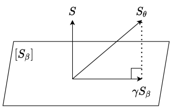
Figure 2: Illustration of the orthogonal score by projection.

Neyman orthogonality.

We use Neyman orthogonality (Neyman, 1959, 1979) to obtain a fast rate for the excess risk. The intuition behind it is that we want the risk to be insensitive to perturbations in the nuisance $g$ so that a good estimate $\hat{\theta}$ can be obtained even if $\hat{g}$ is of poor quality.

Definition 3.

We say the population risk $L$ is Neyman orthogonal at $(\theta_{\star},g_{0})$ over $\Theta^{\prime}\times\mathcal{G}^{\prime}$ if

$$\mathrm{D}_{g}\mathrm{D}_{\theta}L(\theta_{\star},g_{0})[\theta-\theta_{\star},g-g_{0}]=0,\quad\mbox{for all }\theta\in\Theta^{\prime},g\in\mathcal{G}^{\prime}.$$ (4)

Since (4) also implies that $\mathrm{D}_{g}S(\theta_{\star},g_{0})[g-g_{0}]=0$ for all $g\in\mathcal{G}^{\prime}$, we will also say the score $S$ is Neyman orthogonal at $(\theta_{\star},g_{0})$.

When $g$ is parametrized by a finite-dimensional vector $\beta$, we can obtain a Neyman orthogonal score by projection. Let $L(\theta,\beta)$ be some population risk which may not be Neyman orthogonal. We project $S_{\theta}:=\nabla_{\theta}L(\theta,\beta)$ onto the space spanned by $S_{\beta}:=\nabla_{\beta}L(\theta,\beta)$ and obtain $S:=S_{\theta}-\gamma S_{\beta}$ where $\gamma:=[\nabla_{\theta}\nabla_{\beta}L(\theta,\beta)][\nabla^{2}_{\beta}L(\theta,\beta)^{-1}]$. It can be shown that $S$ is Neyman orthogonal at $(\theta_{\star},\beta_{0})$. This procedure is illustrated in Figure 2. Now, to get a population risk that satisfies Neyman orthogonality, it suffices to take the integral of $S$ w.r.t. $\theta$.

2.2 Assumptions

Since our analysis is local to neighborhoods of $\theta_{\star}$ and $g_{0}$, our first assumption localizes the estimator $\hat{\theta}$ and $\hat{g}$ to such neighborhoods.

Assumption 1 (Localization).

Let $r_{1},r_{2}>0$ be constants and $\bar{r}_{1}:=r_{1}\sqrt{\lambda_{\min}(H_{\star})}>0$. There exists a function $N_{\bar{r}_{1},r_{2}}:[0,1]\rightarrow{\mathbb{N}}_{+}$ and such that for any $\delta\in(0,1)$ we have, with probability at least $1-\delta$, $\hat{\theta}\in\Theta_{\bar{r}_{1}}(\theta_{\star})$ and $\hat{g}\in\mathcal{G}_{r_{2}}(g_{0})$ for all $n\geq N_{\bar{r}_{1},r_{2}}(\delta)$.

The localization assumption is necessary to avoid a global strong convexity assumption which is assumed by Foster and Syrgkanis (2020). In order to control the empirical score, we assume that the normalized score at $\theta_{\star}$ is sub-Gaussian uniformly over $\mathcal{G}_{r_{2}}(g_{0})$.

Assumption 2 (Score sub-Gaussianity).

There exists a constant $K_{1}>0$ such that, for every $g\in\mathcal{G}_{r_{2}}(g_{0})$, we have $\left\lVert G(\theta_{\star},g)^{-1/2}[S(\theta_{\star},g;Z)-S(\theta_{\star},g)]\right\rVert_{\psi_{2}}\leq K_{1}$, where $\left\lVert\cdot\right\rVert_{\psi_{2}}$ is the sub-Gaussian norm defined in Appendix C.

Another quantity that we need to control is $S(\theta_{\star},\hat{g})^{\top}(\hat{\theta}-\theta_{\star})=\mathrm{D}_{\theta}L(\theta_{\star},\hat{g})[\hat{\theta}-\theta_{\star}]$. Note that $S(\theta_{\star},g_{0})=0$ by the first order optimality condition. Hence, we may control it with a smoothness assumption on the population risk.

Assumption 3a.

For all $\theta\in\Theta_{\bar{r}_{1}}(\theta_{\star})$ and $g,\bar{g}\in\mathcal{G}_{r_{2}}(g_{0})$, it holds that

$$\left|\mathrm{D}_{g}\mathrm{D}_{\theta}L(\theta_{\star},\bar{g})[\theta-\theta_{\star},g-g_{0}]\right|\leq\beta_{1}\left\lVert\theta-\theta_{\star}\right\rVert_{H_{\star}}\left\lVert g-g_{0}\right\rVert_{\mathcal{G}}$$

for some constant $\beta_{1}>0$.

As we will show in Section 2, this assumption will lead to a slow rate which scales as $O(n^{-1}+\left\lVert\hat{g}-g_{0}\right\rVert_{\mathcal{G}}^{2})$. If $S(\theta_{\star},g)$ is insensitive to $g$ around $g_{0}$, we can obtain a faster rate $O(n^{-1}+\left\lVert\hat{g}-g_{0}\right\rVert_{\mathcal{G}}^{4})$. This insensitivity can be characterized by the Neyman orthogonality and higher order smoothness.

Assumption 3b.

The population risk $L$ is Neyman orthogonal at $(\theta_{\star},g_{0})$ over $\Theta_{\bar{r}_{1}}(\theta_{\star})\times\mathcal{G}_{r_{2}}(g_{0})$. Moreover, it holds for some constant $\beta_{2}>0$ that

$$\left|\mathrm{D}_{g}^{2}\mathrm{D}_{\theta}L(\theta_{\star},\bar{g})[\theta-\theta_{\star},g-g_{0},g-g_{0}]\right|\leq\beta_{2}\left\lVert\theta-\theta_{\star}\right\rVert_{H_{\star}}\left\lVert g-g_{0}\right\rVert_{\mathcal{G}}^{2}$$

for all $\theta\in\Theta_{\bar{r}_{1}}(\theta_{\star})$ and $g,\bar{g}\in\mathcal{G}_{r_{2}}(g_{0})$.

To facilitate the control of the empirical Hessian, we use the pseudo self-concordance as in Definition 2, which allows us to relate $H_{n}(\theta,g)$ and $H(\theta,g)$ to $H_{n}(\theta_{\star},g)$ and $H(\theta_{\star},g)$, respectively.

Assumption 4 (Uniform pseudo self-concordance).

For any $z\in\mathcal{Z}$ and $g\in\mathcal{G}_{r_{2}}(g_{0})$, $\ell(\cdot,g;z)$ is pseudo self-concordant with parameter $R$ on $\Theta_{\bar{r}_{1}}(\theta_{\star})$. Consequently, for any $g\in\mathcal{G}_{r_{2}}(g_{0})$, $L(\cdot,g)$ is pseudo self-concordant with parameter $R$ on $\Theta_{\bar{r}_{1}}(\theta_{\star})$.

Since $\hat{\theta}$ is random, we assume that the Hessian satisfies the Bernstein condition so that we can use a covering number argument to relate $H_{n}(\hat{\theta},g)$ to $H(\theta_{\star},g)$. Due to the variability in $\hat{g}$, the Bernstein condition is satisfied uniformly over a neighborhood of $g_{0}$ and we also assume the stability of $H(\theta_{\star},g)$ around $g_{0}$.

Assumption 5.

For any $\theta\in\Theta_{\bar{r}_{1}}(\theta_{\star})$ and $g\in\mathcal{G}_{r_{2}}(g_{0})$, the centered sandwich Hessian

$$H(\theta,g)^{-1/2}H(\theta,g;Z)H(\theta,g)^{-1/2}-I_{d}$$

satisfies a Bernstein condition with parameter $K_{2}$ and

$$\sigma_{H}^{2}:=\sup_{\theta\in\Theta_{\bar{r}_{1}}(\theta_{\star}),g\in\mathcal{G}_{r_{2}}(g_{0})}\left|\operatorname{\mathbb{V}ar}\left(H(\theta,g)^{-1/2}H(\theta,g;Z)H(\theta,g)^{-1/2}\right)\right|_{2}<\infty,$$

where, for a matrix $J\in{\mathbb{R}}^{d\times d}$, we define $\left|J\right|_{2}:=\max\{\lambda_{\max}(J),\left|\lambda_{\min}(J)\right|\}$ and $\operatorname{\mathbb{V}ar}(J):=\operatorname{\mathbb{E}}[JJ^{\top}]-\operatorname{\mathbb{E}}[J]\operatorname{\mathbb{E}}[J]^{\top}$. Moreover, there exist constants $\kappa$ and $\mathcal{K}$ depending on $r_{2}$ such that

$$\kappa H_{\star}\preceq H(\theta_{\star},g)\preceq\mathcal{K}H_{\star},\quad\mbox{for all }g\in\mathcal{G}_{r_{2}}(g_{0}).$$ (5)

2.3 Main Results

We now present our main results. We will discuss our results in more detail in Section 3. The first result is a fast rate of convergence for the excess risk assuming Neyman orthogonality.

Theorem 1 (Fast rate).

Under Assumptions 1, 2, 3b, 4, and 5, the OSL estimator $\hat{\theta}$ has excess risk, with probability at least $1-\delta$,

$$\mathcal{E}(\hat{\theta},g_{0})\lesssim\frac{e^{3Rr_{1}}}{\kappa^{2}}\left[\frac{K_{1}^{2}\log{(1/\delta)}\bar{d}_{\star}}{n}+\beta_{2}^{2}\left\lVert\hat{g}-g_{0}\right\rVert_{\mathcal{G}}^{4}\right]$$ (6)

whenever $n\geq\max\{N_{\bar{r}_{1},r_{2}}(\delta/5),16(K_{2}^{2}+2\sigma_{H}^{2})[\log{(20d/\delta)}+d\log{(3Rr_{1}/\log{2})}]^{2}\}$, where $\lesssim$ hides an absolute constant.

When Neyman orthogonality fails to hold, we have a similar bound with $\left\lVert\hat{g}-g_{0}\right\rVert_{\mathcal{G}}^{4}$ being replaced by $\left\lVert\hat{g}-g_{0}\right\rVert_{\mathcal{G}}^{2}$.

Theorem 2 (Slow rate).

Under Assumptions 1, 2, 3a, 4, and 5, the OSL estimator $\hat{\theta}$ has excess risk, with probability at least $1-\delta$,

$$\mathcal{E}(\hat{\theta},g_{0})\lesssim\frac{e^{3Rr_{1}}}{\kappa^{2}}\left[\frac{K_{1}^{2}\log{(1/\delta)}\bar{d}_{\star}}{n}+\beta_{1}^{2}\left\lVert\hat{g}-g_{0}\right\rVert_{\mathcal{G}}^{2}\right]$$ (7)

whenever $n\geq\max\{N_{\bar{r}_{1},r_{2}}(\delta/5),16(K_{2}^{2}+2\sigma_{H}^{2})[\log{(20d/\delta)}+d\log{(3Rr_{1}/\log{2})}]^{2}\}$, where $\lesssim$ hides an absolute constant.

The detailed proofs of Theorems 1 and 2 are deferred to Appendix B. On a high level, the proofs proceed as follows. To begin with, due to Assumption 1, we can dedicate our analysis to the case when $\hat{\theta}\in\Theta_{\bar{r}_{1}}(\theta_{\star})$. By Taylor’s theorem,

$$\mathcal{E}(\hat{\theta},g_{0}):=L(\hat{\theta},g_{0})-L(\theta_{\star},g_{0})=S(\theta_{\star},g_{0})^{\top}(\hat{\theta}-\theta_{\star})+\frac{1}{2}\left\lVert\hat{\theta}-\theta_{\star}\right\rVert_{H(\bar{\theta},g_{0})}^{2}$$

for some $\bar{\theta}\in\mbox{Conv}\{\hat{\theta},\theta_{\star}\}$. By the first order orthogonality condition, it holds that $S(\theta_{\star},g_{0})=0$. For the second term, it follows from the property of the pseudo self-concordance (4) that

$$\left\lVert\hat{\theta}-\theta_{\star}\right\rVert_{H(\bar{\theta},g_{0})}^{2}\leq e^{R\left\lVert\bar{\theta}-\theta_{\star}\right\rVert_{2}}\left\lVert\hat{\theta}-\theta_{\star}\right\rVert_{H_{\star}}^{2}\leq e^{Rr_{1}}\left\lVert\hat{\theta}-\theta_{\star}\right\rVert_{H_{\star}}^{2}.$$

It now remains to control $\left\lVert\hat{\theta}-\theta_{\star}\right\rVert_{H_{\star}}^{2}$.

By Taylor’s theorem again, it holds that

$$L_{n}(\hat{\theta},\hat{g})-L_{n}(\theta_{\star},\hat{g})=S_{n}(\theta_{\star},\hat{g})^{\top}(\hat{\theta}-\theta_{\star})+\frac{1}{2}\left\lVert\hat{\theta}-\theta_{\star}\right\rVert^{2}_{H_{n}(\bar{\theta}^{\prime},\hat{g})},$$ (8)

where $\bar{\theta}^{\prime}\in\mbox{Conv}\{\hat{\theta},\theta_{\star}\}$. By the optimality of $\hat{\theta}$, we have $L_{n}(\hat{\theta},\hat{g})-L_{n}(\theta_{\star},\hat{g})\leq 0$. We then lower bound the right hand side of (8). According to Assumption 1, we have $\hat{g}\in\mathcal{G}_{r_{2}}(g_{0})$ with high probability when $n$ is sufficiently large. The following Lemma 3, which is a direct consequence of the independence between $\{Z_{i}\}_{i=1}^{n}$ and $\hat{g}$, allows us to work with fixed $g\in\mathcal{G}_{r_{2}}(g_{0})$ instead of the random estimator $\hat{g}$.

Lemma 3.

Let $\mathcal{A}(\hat{g},\{Z_{i}\}_{i=1}^{n})$ be some event regarding $\hat{g}$ and $\{Z_{i}\}_{i=1}^{n}$. Let $\mathcal{G}^{\prime}\subset\mathcal{G}$. If there exists $\delta\in(0,1)$ such that $\operatorname{\mathbb{P}}(\mathcal{A}(g,\{Z_{i}\}_{i=1}^{n}))\geq 1-\delta$ for all fixed $g\in\mathcal{G}^{\prime}$, then $\operatorname{\mathbb{P}}(\mathcal{A}(\hat{g},\{Z_{i}\}_{i=1}^{n}))\geq(1-\delta)\operatorname{\mathbb{P}}(\hat{g}\in\mathcal{G}^{\prime})$.

Now we focus on the score term $S_{n}(\theta_{\star},g)^{\top}(\hat{\theta}-\theta_{\star})$ in (8) with $\hat{g}$ replaced by a fixed $g\in\mathcal{G}_{r_{2}}(g_{0})$. We split it into two terms

$$[S_{n}(\theta_{\star},g)-S(\theta_{\star},g)]^{\top}(\hat{\theta}-\theta_{\star})+S(\theta_{\star},g)^{\top}(\hat{\theta}-\theta_{\star}).$$ (9)

The first term in (9) can be controlled using the sub-Gaussianity of the score. Recall that

$$\bar{d}_{\star}:=\sup_{g\in\mathcal{G}_{r_{2}}(g_{0})}\operatorname{\bf Tr}(H_{\star}^{-1/2}G(\theta_{\star},g)H_{\star}^{-1/2}).$$

Proposition 4.

Under Assumption 2, it holds for any fixed $g\in\mathcal{G}_{r_{2}}(g_{0})$ that, with probability at least $1-\delta$,

$$\left\lVert S_{n}(\theta_{\star},g)-S(\theta_{\star},g)\right\rVert_{H_{\star}^{-1}}^{2}\lesssim\frac{K_{1}^{2}\log{(1/\delta)}\bar{d}_{\star}}{n}.$$

We handle the second term in (9) by Neyman orthogonality and smoothness assumptions.

Lemma 5.

Under 3b, it holds that

$$S(\theta_{\star},g)^{\top}(\theta-\theta_{\star})\geq-\frac{\beta_{2}}{2}\left\lVert\theta-\theta_{\star}\right\rVert_{H_{\star}}\left\lVert g-g_{0}\right\rVert_{\mathcal{G}}^{2},\quad\mbox{for all }\theta\in\Theta_{\bar{r}_{1}}(\theta_{0})\mbox{ and }g\in\mathcal{G}_{r_{2}}(g_{0}).$$

By Proposition 4 and Lemma 5, we have

$$S_{n}(\theta_{\star},g)^{\top}(\hat{\theta}-\theta_{\star}) \geq-\left\lVert S_{n}(\theta_{\star},g)-S(\theta_{\star},g)\right\rVert_{H_{\star}^{-1}}\left\lVert\hat{\theta}-\theta_{\star}\right\rVert_{H_{\star}}+S(\theta_{\star},g)^{\top}(\hat{\theta}-\theta_{\star})$$

$$\gtrsim-\sqrt{\frac{K_{1}^{2}\log{(1/\delta)}\bar{d}_{\star}}{n}}\left\lVert\hat{\theta}-\theta_{\star}\right\rVert_{H_{\star}}-\beta_{2}\left\lVert\hat{\theta}-\theta_{\star}\right\rVert_{H_{\star}}\left\lVert\hat{g}-g_{0}\right\rVert_{\mathcal{G}}^{2}.$$ (10)

For the Hessian term, with $\hat{g}$ replaced by $g$, $\lVert\hat{\theta}-\theta_{\star}\rVert_{H_{n}(\bar{\theta},g)}$ in (8), we control it using pseudo self-concordance and a covering number argument.

Proposition 6.

Under Assumptions 4 and 5, it holds, with probability at least $1-\delta$, that

$$\frac{\kappa}{4e^{Rr_{1}}}H_{\star}\preceq H_{n}(\theta,g)\preceq 3\mathcal{K}e^{Rr_{1}}H_{\star},\quad\mbox{for all }\theta\in\Theta_{\bar{r}_{1}}(\theta_{\star}),g\in\mathcal{G}_{r_{2}}(g_{0}),$$

whenever $n\geq 16(K_{2}^{2}+2\sigma_{H}^{2})[\log{(4d/\delta)}+d\log{(3Rr_{1}/\log{2})}]^{2}$.

As a consequence of Proposition 6, we have

$$\frac{1}{2}\left\lVert\hat{\theta}-\theta_{\star}\right\rVert_{H_{n}(\bar{\theta},g)}^{2}\gtrsim\frac{\kappa}{e^{Rr_{1}}}\left\lVert\hat{\theta}-\theta_{\star}\right\rVert_{H_{\star}}^{2}.$$ (11)

Putting together (8), (2.3) and (11) leads to an upper bound on $\lVert\hat{\theta}-\theta_{\star}\rVert_{H_{\star}}$ and thus an upper bound on the excess risk $\mathcal{E}(\hat{\theta},g_{0})$.

When Neyman orthogonality fails to hold, we can replace Lemma 5 by the following lemma and repeat the above steps to obtain the slow rate.

Lemma 7.

Under 3a, it holds that

$$S(\theta_{\star},g)^{\top}(\theta-\theta_{\star})\geq-\beta_{1}\left\lVert\theta-\theta_{\star}\right\rVert_{H_{\star}}\left\lVert g-g_{0}\right\rVert_{\mathcal{G}},\quad\mbox{for all }\theta\in\Theta_{\bar{r}_{1}}(\theta_{0})\mbox{ and }g\in\mathcal{G}_{r_{2}}(g_{0}).$$

3 Discussion

Table 1: In its simplest version (e.g., ignoring the effect of $\hat{g}$), our bound scales as $O(d_{\star}/n)$ where $d_{*}:=\operatorname{\bf Tr}(H_{*}^{-1/2}G_{*}H_{*}^{-1/2})$ is the effective dimension, while the bound of Foster and Syrgkanis (2020) scales as $O(d^{\prime}/n)$ where $d^{\prime}:=d^{2}/\lambda_{\min}(H_{\star})$. We compare the two in different regimes of eigendecays of $G_{*}$ and $H_{*}$ assuming they share the same eigenvectors.

	Eigendecay		Dimension Dependency		Ratio
	$G_{\star}$	$H_{\star}$	$d_{\star}$	$d^{\prime}$	$d^{\prime}/d_{\star}$
Poly-Poly	$i^{-\alpha}$	$i^{-\beta}$	$d^{(\beta-\alpha+1)\vee 0}$	$d^{\beta+2}$	$d^{(\alpha+1)\wedge(\beta+2)}$
Poly-Exp	$i^{-\alpha}$	$e^{-\nu i}$	$d^{-(\alpha-1)\vee 1}e^{\nu d}$	$d^{2}e^{\nu d}$	$d^{1\wedge(3-\alpha)}$
Exp-Poly	$e^{-\mu i}$	$i^{-\beta}$	$1$	$d^{\beta+2}$	$d^{\beta+2}$
Exp-Exp	$e^{-\mu i}$	$e^{-\nu i}$	$d$ if $\mu=\nu$   $1$ if $\mu>\nu$ $e^{(\nu-\mu)d}$ if $\mu<\nu$	$d^{2}e^{\nu d}$	$de^{\nu d}$ if $\mu=\nu$ $d^{2}e^{\nu d}$ if $\mu>\nu$ $d^{2}e^{\mu d}$ if $\mu<\nu$

Convergence rate and effective dimension.

There are two terms in the bounds (6) and (7). In the case of no nuisance parameter, the second term involving $\left\lVert\hat{g}-g\right\rVert_{\mathcal{G}}$ vanishes. As for the first term, the profile effective dimension $\bar{d}_{\star}$ simplifies to $d_{\star}:=\operatorname{\bf Tr}(H_{\star}^{-1/2}G_{\star}H_{\star}^{-1/2})$ as shown in Appendix A. This coincides with the result from Ostrovskii and Bach (2021) on generalized linear models, i.e., the loss is given by $\ell(\theta;Z):=\ell(Y,X^{\top}\theta)$. Under a well-specified model, the effective dimension $d_{\star}$ becomes $d$, recovering the same rate $O(d/n)$ as in classical parametric least-squares regression (see, e.g.  Bach, 2021, Proposition 3.5). When the model is misspecified, the effective dimension measures the mismatch between the covariance matrix $G_{\star}$ and the Hessian matrix $H_{\star}$. This quantity is related to the sandwich covariance in statistics (Wakefield, 2013, Sec. 6.7).

To facilitate its understanding, we summarize the effective dimension $d_{\star}$ in Table 1 under different regimes of eigendecay, assuming that $G_{\star}$ and $H_{\star}$ share the same eigenvectors. Table 1 shows that the dimension dependence can be better than $O(d)$ when the spectrum of $G_{\star}$ decays faster than the one of $H_{\star}$. In particular, it is most favorable when the spectrum of $G_{\star}$ decays as $e^{-\mu i}$ and the one of $H_{\star}$ decays as $i^{-\beta}$.

In the case when the nuisance parameter needs to be estimated, we pay the price of not knowing the true nuisance in both of the two terms. In this first term, we have $\bar{d}_{\star}$ rather than $d_{\star}$ which is the maximum effective dimension in a neighborhood of $g_{0}$. As for the second term, the estimator $\hat{g}$ will typically have a rate of convergence $\left\lVert\hat{g}-g_{0}\right\rVert_{\mathcal{G}}=O(n^{-\varphi})$ with $\varphi<1/2$ in high dimensions (Chernozhukov et al., 2018, Section 1). As a result, the term $\left\lVert\hat{g}-g_{0}\right\rVert_{\mathcal{G}}^{2}$ has a dominating effect in the bound (7) which is slower than $O(n^{-1})$. If Neyman orthogonality holds as assumed in Theorem 1, we do not pay this price in the fast rate (6) as long as $\varphi\geq 1/4$. Note that Neyman orthogonality is only used in Lemma 5 to control $S(\theta_{\star},g)^{\top}(\theta-\theta_{\star})$. If $\lvert\mathrm{D}_{g}\mathrm{D}_{\theta}L(\theta_{\star},g_{0})[\hat{\theta}-\theta_{\star},\hat{g}-g_{0}]\rvert$ does not vanish but decays as $O(r_{n})$, then the second term in (6) will read $O(r_{n}^{2}+\left\lVert\hat{g}-g_{0}\right\rVert_{\mathcal{G}}^{4})$.

Orthogonal statistical learning and double machine learning.

Our work lies in the framework of orthogonal statistical learning. Under a strong convexity assumption and a Neyman orthogonality assumption on the population risk, Foster and Syrgkanis (2020) obtain the rate

$$\mathcal{E}(\hat{\theta},g_{0})\lesssim O\left(\frac{d^{2}}{n\lambda^{2}}+\frac{d}{\lambda^{2}}\left\lVert\hat{g}-g_{0}\right\rVert_{\mathcal{G}}^{4}\right),\quad\mbox{for all }n\geq 1,$$ (12)

where $\lambda$ is the infimum of $\lambda_{\min}(H(\theta,g_{0}))$ over a neighborhood of $\theta_{\star}$ (see Foster and Syrgkanis, 2020, Theorems 1 and 3). Our results improve on theirs in several ways. When $\bar{d}_{\star}$ is at most proportional to the dimension $d$, our results improve the excess risk bound by at least a factor of $d$. Our bounds also remove the explicit dependence on the minimum eigenvalue $\lambda$, owing to our tail assumptions 2 and 5 on the normalized score and the Hessian. However, our bounds may depend on $\lambda$ implicitly through, e.g., the sub-Gaussian parameter $K_{1}$. This dependency contributes at most a factor of $\lambda^{-1}$ for applications considered in Section 4. Hence, to be more concrete, we compare $d_{\star}$ with $d^{2}/\lambda_{\min}(H_{\star})$ in different eigendecay regimes in Table 1. For instance, when the spectrum of $G_{\star}$ decays as $e^{-\mu i}$ and the one of $H_{\star}$ decays as $i^{-\beta}$, our bound gives a rate $O(n^{-1})$ while theirs gives a rate $O(d^{\beta+2}/n)$.

Chernozhukov et al. (2018) recently proposed a set of methods based on Neyman orthogonal scores and cross-fitting, denoted by double or debiased machine learning (DML), to the classical problem of semi-parametric inference. There is an abundant literature on semi-parametric estimation in mathematical statistics (Xia and Härdle, 2006; Wellner and Zhang, 2007) and machine learning (Smola et al., 1998; Rakotomamonjy et al., 2005; Mackey et al., 2018; Bertail et al., 2021) and we refer to classical books for a bibliography (Bickel et al., 1998; Ruppert et al., 2003; Tsiatis, 2006; Kosorok, 2008; Van der Laan and Rose, 2011). In Chernozhukov et al. (2018), the authors establish the asymptotic normality of their estimators when the dimension of the target parameter is kept fixed. In this work, we provide non-asymptotic guarantees in terms of excess risk for DML under self-concordance, allowing the dimension of the target parameter to grow at the rate $d=O(n^{1/2})$. In a recent work (Nekipelov et al., 2022), regularized estimators with sparsity-inducing regularization are analyzed in terms of parameter recovery under restricted convexity assumptions.

4 Applications and Examples

4.1 Treatment Effect Estimation

Let us revisit the problem of treatment effect estimation under the assumption of unconfoundedness, as presented in the introduction. Before we had a binary treatment case, and our target of inference was a one dimensional parameter. Here, to better fit our framework, we consider a vector of predictors $D:=(D^{k})_{k=1}^{d}\in\mathbb{R}^{d}$, under partially linear CEF of the following form:

$$\operatorname{\mathbb{E}}[Y\mid D,X]=\theta_{0}^{\top}D+\gamma_{0}(X).$$

Note that, by targeting multiple coefficients $\theta\in\Theta\subset\mathbb{R}^{d}$, we can model not only multiple treatments, but also heterogeneous treatment effects across different binary groups, as well as other non-linear effects, by performing nonlinear transformations of our original treatment variable. To illustrate, suppose $T$ is the original treatment and there is a finite dimensional feature map $D:=\phi(T)=[\phi_{1}(T),\dots,\phi_{d}(T)]$ such that $\operatorname{\mathbb{E}}[Y\mid T,X]=\theta_{0}^{\top}\phi(T)+\gamma_{0}(X)$. Under the the assumption of uncounfoundedness conditional on $X$, the ATE of setting $T$ to $t_{1}$ versus $t_{0}$ is then given by:

$$\operatorname{\mathbb{E}}[Y(T=t_{1})-Y(T=t_{0})]=\theta_{0}^{\top}(\phi(t_{1})-\phi(t_{0})).$$

Heterogeneous effects could be estimated in a similar manner. Letting $G=[G_{1},\dots,G_{d}]$ denote indicators for $d$ subgroups, and letting $T\in\{0,1\}$ denote the binary treatment indicator, we can define the covariates $D:=TG$. With this flexibility in mind, we now examine the partially linear model in the context of our framework.

Multiple target coefficients in a partially linear model.

Let the “target” predictors be $D:=(D^{k})_{k=1}^{d}\in\mathbb{R}^{d}$. Consider the model

$$D =\alpha_{0}(X)+U$$

$$Y =\theta_{0}^{\top}D+\gamma_{0}(X)+V=\zeta_{0}(X)+\theta_{0}^{\top}U+V,$$

where $\alpha_{0}:{\mathbb{R}}^{p}\rightarrow{\mathbb{R}}^{d}$, $\operatorname{\mathbb{E}}[U\mid X]\overset{\mbox{\scriptsize a.s.}}{=}0$ and $\operatorname{\mathbb{E}}[V\mid D,X]\overset{\mbox{\scriptsize a.s.}}{=}0$ are the residuals. Moreover, $U$ has a non-singular covariance $\Sigma_{u}$ and $V$ is independent of $D$ and $X$ with variance $\sigma_{v}^{2}>0$. We reparametrize the model by $g=(\zeta,\alpha)$ and work with the loss

$$\ell(\theta,g;Z):=[Y-\zeta(X)-\theta^{\top}(D-\alpha(X))]^{2}.$$

Since $\operatorname{\mathbb{E}}[UV]=\operatorname{\mathbb{E}}[(D-\alpha_{0}(X))V]=0$, we have

$$L(\theta,g) :=\operatorname{\mathbb{E}}[[Y-\zeta(X)-\theta^{\top}(D-\alpha(X))]^{2}]$$

$$=\operatorname{\mathbb{E}}\left[\left(\zeta_{0}(X)-\zeta(X)-\theta^{\top}(\alpha_{0}(X)-\alpha(X))\right)^{2}\right]+\left\lVert\theta-\theta_{0}\right\rVert_{\Sigma_{u}}^{2}+\sigma_{v}^{2}.$$

This implies that the population risk $L$ at $g_{0}$ has a unique minimizer $\theta_{\star}=\theta_{0}$.

Now suppose that $U$ is bounded (i.e., $\left\lVert U\right\rVert_{2}\leq M$), $V$ is sub-Gaussian with parameter $\left\lVert V\right\rVert_{\psi_{2}}$, and $\left\lVert\cdot\right\rVert_{\mathcal{G}}$ is chosen as the sup-norm, i.e., $\left\lVert g\right\rVert_{\mathcal{G}}=\sup_{x}\sqrt{\left\lVert\alpha(x)\right\rVert^{2}+\zeta^{2}(x)}$. Let us verify the assumptions in Section 2.2 for this model. For Assumption 2, we have

$$S(\theta_{\star},g;Z) =2(\alpha_{0}(X)-\alpha(X)+U)\left[(\alpha_{0}(X)-\alpha(X))^{\top}\theta_{\star}-(\zeta_{0}(X)-\zeta(X)+V)\right],$$

$$S(\theta_{\star},g) =2\operatorname{\mathbb{E}}\left[(\alpha_{0}(X)-\alpha(X))(\alpha_{0}(X)-\alpha(X))^{\top}\theta_{\star}-(\alpha_{0}(X)-\alpha(X))(\zeta_{0}(X)-\zeta(X))\right],$$

and $G(\theta_{\star},g)\succeq 4\sigma_{v}^{2}\Sigma_{u}$. Note that $\left\lVert\alpha_{0}(X)-\alpha(X)\right\rVert\leq\left\lVert g-g_{0}\right\rVert_{\mathcal{G}}\leq r_{2}$, $\left\lVert\zeta_{0}(X)-\zeta(X)\right\rVert\leq\left\lVert g-g_{0}\right\rVert_{\mathcal{G}}\leq r_{2}$, $\left\lVert U\right\rVert_{2}\leq M$, and $V$ is sub-Gaussian. Hence, it follows from Lemmas 11,12 and 13 that the normalized score is sub-Gaussian with sub-Gaussian norm

$$K_{1}\lesssim\frac{(r_{2}+M)[r_{2}(\left\lVert\theta_{\star}\right\rVert_{2}+1)+\left\lVert V\right\rVert_{\psi_{2}}]}{\sigma_{v}\sqrt{\lambda_{\min}(\Sigma_{u})}}.$$

For 3b, it holds that, for any $\bar{\theta}\in\Theta$,

$$\mathrm{D}_{g}\mathrm{D}_{\theta}L(\bar{\theta},g_{0})[\theta-\theta_{\star},g-g_{0}]\equiv 0,$$

which verifies the Neyman orthogonality. Moreover, we have $H_{\star}=\nabla_{\theta}^{2}L(\theta_{\star},g_{0})=2\Sigma_{u}$ and

$$\quad\left|\mathrm{D}_{g}^{2}\mathrm{D}_{\theta}L(\theta_{\star},\bar{g})[\theta-\theta_{\star},g-g_{0},g-g_{0}]\right|$$

$$=\left|4(\theta-\theta_{\star})^{\top}\operatorname{\mathbb{E}}\left\{(\alpha_{0}(X)-\alpha(X))\left[(\alpha_{0}(X)-\alpha(X))^{\top}\theta_{\star}-(\zeta_{0}(X)-\zeta(X))\right]\right\}\right|$$

$$\lesssim\frac{\left\lVert\theta_{\star}\right\rVert_{2}+1}{\sqrt{\lambda_{\min}(\Sigma_{u})}}\left\lVert\theta-\theta_{\star}\right\rVert_{H_{\star}}\left\lVert g-g_{0}\right\rVert_{\mathcal{G}}^{2}.$$

In other words, 3b holds true with $\beta_{2}\lesssim(\left\lVert\theta_{\star}\right\rVert_{2}+1)/\sqrt{\lambda_{\min}(\Sigma_{u})}$.

For 4, both the loss $\ell$ and the population risk $L$ are pseudo self-concordant with arbitrary parameter $R\geq 0$ since their third derivatives w.r.t. $\theta$ are zero. For 5, we have

$$H(\theta,g;Z) =2(\alpha_{0}(X)-\alpha(X)+U)(\alpha_{0}(X)-\alpha(X)+U)^{\top},$$

$$H(\theta,g) =2\operatorname{\mathbb{E}}[(\alpha_{0}(X)-\alpha(X)+U)(\alpha_{0}(X)-\alpha(X)+U)^{\top}]\succeq 2\Sigma_{u}.$$

Note that $H(\theta,g)^{-1/2}H(\theta,g;Z)H(\theta,g)^{-1/2}-I_{d}$ has mean-zero and satisfies

$$\left|H(\theta,g)^{-1/2}H(\theta,g;Z)H(\theta,g)^{-1/2}-I_{d}\right|_{2}\lesssim\left\lVert H(\theta,g)^{-1}\right\rVert_{2}[\left\lVert g-g_{0}\right\rVert_{\mathcal{G}}^{2}+\left\lVert U\right\rVert_{2}^{2}]\lesssim\frac{r_{2}^{2}+M^{2}}{\lambda_{\min}(\Sigma_{u})}.$$

Hence, it follows from Wainwright (2019, Equation 6.30) that

$$H(\theta,g)^{-1/2}H(\theta,g;Z)H(\theta,g)^{-1/2}-I_{d}$$

satisfies the Bernstein condition with parameter $K_{2}\lesssim(r_{2}^{2}+M^{2})/\lambda_{\min}(\Sigma_{u})$. Moreover, $\sigma_{H}^{2}\lesssim(r_{2}^{2}+M^{2})^{2}/\lambda_{\min}^{2}(\Sigma_{u})$. For the stability (5), we have $H_{\star}=2\Sigma_{u}$ and

$$2\Sigma_{u}\preceq H(\theta_{\star},g)=2\operatorname{\mathbb{E}}[(\alpha_{0}(X)-\alpha(X)+U)(\alpha_{0}(X)-\alpha(X)+U)^{\top}]\preceq 2[r_{2}^{2}I_{d}+\Sigma_{u}].$$

Thus, the stability holds with $\kappa=1$ and $\mathcal{K}=1+r_{2}^{2}/\lambda_{\min}(\Sigma_{u})$. To summarize, invoking Theorem 1 gives the following risk bound up to a constant factor:

$$\frac{(r_{2}+M)^{2}[r_{2}(\left\lVert\theta_{\star}\right\rVert_{2}+1)+\left\lVert V\right\rVert_{\psi_{2}}]^{2}}{\sigma_{v}^{2}\lambda_{\min}(\Sigma_{u})}\frac{\bar{d}_{\star}}{n}\log{(1/\delta)}+\frac{(\left\lVert\theta_{\star}\right\rVert_{2}+1)^{2}}{\lambda_{\min}(\Sigma_{u})}\left\lVert\hat{g}-g_{0}\right\rVert_{\mathcal{G}}^{4}.$$ (13)

Remark 1.

As a comparison, assuming $\left\lVert U\right\rVert_{2}\leq M$, $\left\lVert V\right\rVert_{2}\leq M^{\prime}$, and $R:=\sup_{\theta\in\Theta}\left\lVert\theta\right\rVert_{2}\vee 1<\infty$, Theorems 1 and 3 of Foster and Syrgkanis (2020) yield the bound

$$\frac{\bar{K}^{2}}{\lambda_{\min}(\Sigma_{u})^{2}}\frac{d^{2}}{n}\log{(1/\delta)}+\frac{R\bar{K}d}{\lambda_{\min}(\Sigma_{u})^{2}}\left\lVert\hat{g}-g_{0}\right\rVert_{\mathcal{G}}^{4},$$

where $\bar{K}:=(r_{2}+M)[r_{2}(R+1)+M^{\prime}+RM]$. Our result not only requires less stringent assumptions but also improves their result by a factor of $d/\lambda_{\min}(\Sigma_{u})$ when $\bar{d}_{\star}\lesssim d$.

4.2 Semi-Parametric Logistic Regression

We consider a semi-parametric logistic regression model to illustrate the usefulness of the pseudo self-concordance assumption.

Let $Z:=(X,W,Y)$ where $X\in{\mathbb{R}}^{d}$, $W\in\mathcal{W}$, and $Y\in\{-1,1\}$. Consider the model

$$\operatorname{\mathbb{P}}(Y=1\mid X,W)=\sigma\left(\theta_{0}^{\top}X+g_{0}(W)\right),$$

where $\sigma(u):=(1+e^{-u})^{-1}$. It is clear that

$$\operatorname{\mathbb{E}}[Y\mid X,W] =\operatorname{\mathbb{P}}(Y=1\mid X,W)-\operatorname{\mathbb{P}}(Y=-1\mid X,W)=2\sigma(\theta_{0}^{\top}X+g_{0}(W))-1.$$

The logistic loss is defined as

$$\ell(\theta,g;Z):=\log{\left(1+\exp\left(-Y(\theta^{\top}X+g(W))\right)\right)}.$$

It can be shown that

$$S(\theta,g;Z)=\left[\sigma(\theta^{\top}X+g(W))-\frac{1}{2}-\frac{Y}{2}\right]X$$

and

$$S(\theta,g) =\operatorname{\mathbb{E}}[\operatorname{\mathbb{E}}[S(\theta,g;Z)\mid X,W]]=\operatorname{\mathbb{E}}\left\{X\left[\sigma(\theta^{\top}X+g(W))-\sigma(\theta_{0}^{\top}X+g_{0}(W))\right]\right\}$$

$$H(\theta,g) =\operatorname{\mathbb{E}}\left[\sigma(\theta^{\top}X+g(W))[1-\sigma(\theta^{\top}X+g(W))]XX^{\top}\right]$$

$$G(\theta,g) =\operatorname{\mathbb{E}}\left\{[\sigma(\theta^{\top}X+g(W))-\sigma(\theta_{0}^{\top}X+g_{0}(W))]^{2}XX^{\top}\right\}-S(\theta,g)S(\theta,g)^{\top}+H(\theta_{0},g_{0}).$$

Assume that $H_{\star}:=H(\theta_{0},g_{0})$ is non-singular. The population risk $L(\theta,g_{0})$ is minimized at $\theta_{\star}=\theta_{0}$.

Suppose that $X$ is bounded (i.e., $\left\lVert X\right\rVert_{2}\leq M$), $r_{1}\leq\lambda_{\min}(H_{\star})/M^{3}$, and $r_{2}\leq\lambda_{\min}(H_{\star})/M^{2}$. By the non-singularity of $H_{\star}$, the covariance $G(\theta,g)$ is non-singular for all $\theta\in\Theta$ and $g\in\mathcal{G}$. Let us verify the assumptions in Section 2.2 for this model. For Assumption 2, it follows directly from Lemmas 11 and 13 that the normalized score is sub-Gaussian with sub-Gaussian norm $K_{1}\lesssim M/\sqrt{\lambda_{\min}(H_{\star})}$. 3a holds true with $\beta_{1}:=M/(4\sqrt{\lambda_{\min}(H_{\star})})$ since

$$\quad\left|\mathrm{D}_{g}\mathrm{D}_{\theta}L(\theta_{\star},\bar{g})[\theta-\theta_{\star},g-g_{0}]\right|$$

$$=\left|\operatorname{\mathbb{E}}\left[\sigma(\theta_{\star}^{\top}X+\bar{g}(W))[1-\sigma(\theta_{\star}^{\top}X+\bar{g}(W))]X^{\top}(\theta-\theta_{\star})(g(W)-g_{0}(W))\right]\right|$$

$$\leq\frac{M}{4\sqrt{\lambda_{\min}(H_{\star})}}\left\lVert\theta-\theta_{\star}\right\rVert_{H_{\star}}\left\lVert g-g_{0}\right\rVert_{\mathcal{G}}.$$

For 4, we have, with $a:=\theta^{\top}x+g(w)$,

$$\left|\mathrm{D}_{\theta}^{3}\ell(\theta,g;z)[u,u,u]\right| =\left|\sigma(a)[1-\sigma(a)][1-2\sigma(a)](u^{\top}x)^{3}\right|$$

$$\leq\left|\sigma(a)[1-\sigma(a)]\left\lVert u\right\rVert_{2}\left\lVert x\right\rVert_{2}(u^{\top}x)^{2}\right|$$

$$\leq M\left\lVert u\right\rVert_{2}\mathrm{D}_{\theta}^{2}\ell(\theta,g;z)[u,u],$$

which implies that $\ell(\cdot,g;z)$ is pseudo self-concordance with parameter $R=M$. The pseudo self-concordance of $L(\theta,g)$ can be verified similarly.

For 5, we first show that $H(\theta,g)$ is non-singular on $\Theta_{\bar{r}_{1}}(\theta_{\star})\times\mathcal{G}_{r_{2}}(g_{0})$. In fact, with $A:=\theta^{\top}X+g(W)$ and $A_{0}:=\theta_{0}^{\top}X+g_{0}(W)$, we have

$$\left|H(\theta,g)-H_{\star}\right|_{2} \leq\operatorname{\mathbb{E}}\left[\left|\sigma(A)-\sigma(A_{0})\right|\left|XX^{\top}\right|_{2}\right]$$

$$\leq\frac{1}{4}\operatorname{\mathbb{E}}\left[[\lvert\theta^{\top}X-\theta_{0}^{\top}X\rvert+\left|g(W)-g_{0}(W)\right|]\left|XX^{\top}\right|_{2}\right]$$

$$\leq\frac{1}{4}\left(r_{1}M^{3}+r_{2}M^{2}\right),\quad\mbox{for all }(\theta,g)\in\Theta_{\bar{r}_{1}}(\theta_{\star})\times\mathcal{G}_{r_{2}}(g_{0}).$$

This yields that

$$\left|H_{\star}^{-1/2}H(\theta,g)H_{\star}^{-1/2}-I_{d}\right|_{2}\leq\frac{1}{4\lambda_{\min}(H_{\star})}\left(r_{1}M^{3}+r_{2}M^{2}\right)\leq\frac{1}{2},$$

and thus $H(\theta,g)\succeq I_{d}/2$ for all $(\theta,g)\in\Theta_{\bar{r}_{1}}(\theta_{\star})\times\mathcal{G}_{r_{2}}(g_{0})$. Analogously, we can show that

$$\left|H_{\star}^{-1/2}H(\theta_{\star},g)H_{\star}^{-1/2}-I_{d}\right|_{2}\leq\frac{r_{2}M^{2}}{4\lambda_{\min}(H_{\star})}\leq\frac{1}{4},$$

and thus the stability (5) holds true with $\kappa=3/4$ and $\mathcal{K}=5/4$. As for the Bernstein condition, we note that

$$\left|H(\theta,g;Z)\right|_{2}=\left|\sigma(\theta^{\top}X+g(W))[1-\sigma(\theta^{\top}X+g(W))]XX^{\top}\right|_{2}\leq\frac{M^{2}}{4}.$$

It follows that

$$\left|H(\theta,g)^{-1/2}H(\theta,g;Z)H(\theta,g)^{-1/2}-I_{d}\right|_{2}\leq\frac{M^{2}}{2\lambda_{\min}(H(\theta,g))}\leq M^{2}.$$

Due to (Wainwright, 2019, Equation 6.30), $H(\theta,g)^{-1/2}H(\theta,g;Z)H(\theta,g)^{-1/2}-I_{d}$ satisfies the Bernstein condition with parameter $K_{2}\lesssim M^{2}$. Moreover, $\sigma_{H}^{2}\lesssim M^{4}$. To summarize, invoking Theorem 2 gives the following risk bound up to a constant factor:

$$\frac{M^{2}}{\lambda_{\min}(H_{\star})}\left[\frac{\bar{d}_{\star}}{n}\log{(1/\delta)}+\left\lVert\hat{g}-g_{0}\right\rVert_{\mathcal{G}}^{2}\right].$$

Remark 2.

Since the semi-parametric logistic loss does not satisfy the Neyman orthogonality, the results of Foster and Syrgkanis (2020) do not directly apply here.

5 Conclusion

We established non-asymptotic guarantees in terms of the excess risk for the orthogonal statistical learning under pseudo self-concordance, allowing the dimension of the target parameter to grow at the rate $d=O(n^{1/2})$. The dimension dependency in our bound is characterized by the effective dimension—the trace of the sandwich covariance matrix—which recovers existing results in supervised learning without the nuisance parameter. Compared with previous work (Foster and Syrgkanis, 2020), our results improve on the excess risk bound at least by a factor of $d$ in a wide range of eigendecay regimes. The extension of our theoretical analysis to handle sparse regularization is an interesting venue for future work.

Acknowledgements

The authors would like to thank Jon Wellner for fruitful discussions. L. Liu is supported by NSF CCF-2019844 and NSF DMS-2023166. Z. Harchaoui is supported by NSF CCF-2019844, NSF DMS-2134012, NSF DMS-2023166, CIFAR-LMB, and faculty research awards. Part of this work was done while Z. Harchaoui was visiting the Simons Institute for the Theory of Computing.

The Appendix is organized as follows. For simplicity, we first prove in Appendix A the main results assuming that the true nuisance parameter $g_{0}$ is known. We then prove in Appendix B the main results presented in Section 2. The technical tools used in the proofs are reviewed and developed in Appendix C.

Appendix A Risk Bound with Known Nuisance Parameter

In this section, we assume that the true nuisance parameter $g_{0}$ is known and control the excess risk. The proofs in this section are inspired by and extend those from Ostrovskii and Bach (2021). We denote by $\hat{\theta}_{0}$ the minimizer of the empirical risk $L_{n}(\theta,g_{0})$. Our analysis is local to $\theta_{\star}$, in other words, we make the following assumption on $\hat{\theta}_{0}$. Recall that $\Theta_{r}(\theta_{\star}):=\{\theta\in\Theta:\left\lVert\theta-\theta_{\star}\right\rVert_{H_{\star}}<r\}$.

Assumption 6.

Let $r_{0}>0$ be a constant and $\tilde{r}_{0}:=\min\{r_{0},r_{0}\sqrt{\lambda_{\min}(H_{\star})}\}>0$. There exists a function $N_{\tilde{r}_{0}}:[0,1]\rightarrow{\mathbb{N}}_{+}$ such that for any $\delta\in(0,1)$ we have, with probability at least $1-\delta$, $\hat{\theta}_{0}\in\Theta_{\tilde{r}_{0}}(\theta_{\star})$ for all $n\geq N_{\tilde{r}_{0}}(\delta)$.

Control of the score.

In order to control the score, we assume that the normalized score at $\theta_{\star}$ is sub-Gaussian.

Assumption 7.

The normalized score at $\theta_{0}$ is sub-Gaussian, i.e., there exists a constant $K_{1,0}>0$ such that

$$\left\lVert G_{\star}^{-1/2}[S(\theta_{\star},g_{0};Z)-S(\theta_{\star},g_{0})]\right\rVert_{\psi_{2}}\leq K_{1,0}.$$

Recall that $d_{\star}:=\operatorname{\bf Tr}(\Omega_{\star})$ and $\Omega_{\star}:=H_{\star}^{-1/2}G_{\star}H_{\star}^{-1/2}$.

Proposition 8.

Under 7, it holds that, with probability at least $1-\delta$,

$$\left\lVert S_{n}(\theta_{\star},g_{0})\right\rVert_{H_{\star}^{-1}}^{2}\lesssim\frac{1}{n}[d_{\star}+K_{1,0}^{2}\log{(e/\delta)}\left\lVert\Omega_{\star}\right\rVert_{2}],$$

where $\lesssim$ hides an absolute constant.

Proof.

By the first order optimality condition, we have $S(\theta_{\star},g_{0})=0$. As a result,

$$X:=\sqrt{n}G_{\star}^{-1/2}S_{n}(\theta_{\star},g_{0};Z)$$

is an isotropic random vector. Moreover, we have $\left\lVert X\right\rVert_{\psi_{2}}\lesssim K_{1,0}$ by Lemma 14. Define $J:=G_{\star}^{1/2}H_{\star}^{-1}G_{\star}^{1/2}/n$. Then we have

$$\left\lVert S_{n}(\theta_{\star},g_{0})\right\rVert_{H_{\star}^{-1}}^{2}=\left\lVert X\right\rVert_{J}^{2}.$$

Invoking Theorem 15 yields the claim. ∎

Control of the Hessian.

In order to control the Hessian, we use the pseudo self-concordance as in Definition 2.

Assumption 8.

For any $z\in\mathcal{Z}$, $\ell(\theta,g_{0};z)$ is pseudo self-concordant on $\Theta_{\tilde{r}_{0}}(\theta_{\star})$, i.e.,

$$\left|\mathrm{D}_{\theta}^{3}\ell(\theta,g_{0};z)[u,u,u]\right|\leq R_{0}\left\lVert u\right\rVert_{2}\mathrm{D}_{\theta}^{2}\ell(\theta,g_{0};z)[u,u],\quad\mbox{for all }\theta\in\Theta_{\tilde{r}_{0}}(\theta_{\star}),u\in{\mathbb{R}}^{d}.$$

Moreover, $L(\theta,g_{0})$ is pseudo self-concordant on $\Theta_{\tilde{r}_{0}}(\theta_{\star})$.

We also assume that the Hessian $H(\theta,g_{0};Z)$ satisfies the Bernstein condition uniformly over $\Theta_{\tilde{r}_{0}}(\theta_{\star})$.

Assumption 9.

For any $\theta\in\Theta_{\tilde{r}_{0}}(\theta_{\star})$, the centered sandwich Hessian

$$H(\theta,g_{0})^{-1/2}H(\theta,g_{0};Z)H(\theta,g_{0})^{-1/2}-I_{d}$$

satisfies a Bernstein condition with parameter $K_{2,0}$. Moreover,

$$\sigma_{H,0}^{2}:=\sup_{\theta\in\Theta_{\tilde{r}_{0}}(\theta_{\star})}\left|\operatorname{\mathbb{V}ar}(H(\theta,g_{0})^{-1/2}H(\theta,g_{0};Z)H(\theta,g_{0})^{-1/2})\right|_{2}<\infty.$$

Proposition 9.

Under 8, for any $\theta\in\Theta_{\tilde{r}_{0}}(\theta_{\star})$, we have

$$e^{-R_{0}r_{0}}H_{\star}\preceq H(\theta,g_{0})\preceq e^{R_{0}r_{0}}H_{\star}.$$ (14)

Moreover, if 9 holds true, then, with probability at least $1-\delta$, we have

$$\frac{1}{4e^{R_{0}r_{0}}}H_{\star}\preceq H_{n}(\theta,g_{0})\preceq 3e^{R_{0}r_{0}}H_{\star},\quad\mbox{for all }\theta\in\Theta_{\tilde{r}_{0}}(\theta_{\star}),$$ (15)

whenever $n\geq 16(K_{2,0}^{2}+2\sigma_{H,0}^{2})\left[\log{(4d/\delta)}+d\log{(3r_{0}R_{0}/\log{2})}\right]^{2}$.

Proof.

According to 8 and Proposition 17, we have

$$e^{-R_{0}\left\lVert\theta-\theta_{\star}\right\rVert_{2}}H_{\star}\preceq H(\theta,g_{0})\preceq e^{R_{0}\left\lVert\theta-\theta_{\star}\right\rVert_{2}}H_{\star}.$$

Hence, the claim (14) follows from $\left\lVert\theta-\theta_{\star}\right\rVert_{2}\leq\tilde{r}_{0}/\sqrt{\lambda_{\min}(H_{\star})}\leq r_{0}$. As for (15), we prove it in the following steps.

Step 1. Let $\epsilon=\sqrt{\lambda_{\min}(H_{\star})}\log{2}/R_{0}$. Take an $\epsilon$-covering $\mathcal{N}_{\epsilon}$ of $\Theta_{\tilde{r}_{0}}(\theta_{\star})$ w.r.t. $\left\lVert\cdot\right\rVert_{H_{\star}}$, and let $\pi(\theta)$ be the projection of $\theta$ onto $\mathcal{N}_{\epsilon}$. By the self-concordance of $\ell(\cdot,g_{0};z)$ (8), we have, for all $\theta\in\Theta_{\tilde{r}_{0}}(\theta_{\star})$,

$$e^{-R_{0}r}H(\pi(\theta),g_{0};Z)\preceq H(\theta,g_{0};Z)\preceq e^{R_{0}r}H(\pi(\theta),g_{0};Z),$$

where $r:=\left\lVert\theta-\pi(\theta)\right\rVert_{2}\leq\epsilon/\sqrt{\lambda_{\min}(H_{\star})}=\log{2}/R_{0}$. It then follows that

$$\frac{1}{2}H(\pi(\theta),g_{0};Z_{i})\preceq H(\theta,g_{0};Z_{i})\preceq 2H(\pi(\theta),g_{0};Z_{i}),\quad\mbox{for all }\theta\in\Theta_{\tilde{r}_{0}}(\theta_{\star})\mbox{ and }i\in[n],$$

which yields

$$\frac{1}{2}H_{n}(\pi(\theta),g_{0})\preceq H_{n}(\theta,g_{0})\preceq 2H_{n}(\pi(\theta),g_{0}),\quad\mbox{for all }\theta\in\Theta_{\tilde{r}_{0}}(\theta_{\star}).$$ (16)

Step 2. By Theorem 16, for each $\theta\in\Theta_{\tilde{r}_{0}}(\theta_{\star})$, it holds that, with probability at least $1-\delta$,

$$\left|H(\theta,g_{0})^{-1/2}H_{n}(\theta,g_{0})H(\theta,g_{0})^{-1/2}-I_{d}\right|_{2}\leq\frac{1}{2},$$

or equivalently,

$$\frac{1}{2}H(\theta,g_{0})\preceq H_{n}(\theta,g_{0})\preceq\frac{3}{2}H(\theta,g_{0})$$

whenever $n\geq 16(K_{2,0}^{2}+2\sigma_{H,0}^{2})\log^{2}{(2d/\delta)}$. Since $\left|\mathcal{N}_{\epsilon}\right|\leq(3\tilde{r}_{0}/\epsilon)^{d}$ (Ostrovskii and Bach, 2021), by a union bound, we get, with probability at least $1-\delta/2$,

$$\frac{1}{2}H(\pi(\theta),g_{0})\preceq H_{n}(\pi(\theta),g_{0})\preceq\frac{3}{2}H(\pi(\theta),g_{0}),\quad\mbox{for all }\theta\in\Theta_{\tilde{r}_{0}}(\theta_{\star}),$$ (17)

whenever $n\geq 16(K_{2,0}^{2}+2\sigma_{H,0}^{2})\left[\log{(4d/\delta)}+d\log{(3r_{0}R_{0}/\log{2})}\right]^{2}$. Hence, the statement (15) follows from (14), (16), and (17). ∎

Control of the excess risk.

The next theorem shows that the excess risk is upper bounded by $d_{\star}/n$ up to a constant factor.

Theorem 10.

Under Assumptions 6-9, with probability at least $1-\delta$, the excess risk of $\hat{\theta}_{0}$ satisfies

$$\mathcal{E}(\hat{\theta}_{0},g_{0})\lesssim K_{1,0}^{2}e^{3R_{0}r_{0}}\log{(1/\delta)}\frac{d_{\star}}{n}$$ (18)

whenever $n\geq\max\{N_{\tilde{r}_{0}}(\delta/3),16(K_{2,0}^{2}+2\sigma_{H,0}^{2})\left[\log{(12d/\delta)}+d\log{(3r_{0}R_{0}/\log{2})}\right]^{2}\}$.

Proof.

We start by defining three events. Let

$$\mathcal{A} :=\left\{\hat{\theta}_{0}\in\Theta_{\tilde{r}_{0}}(\theta_{\star})\right\}$$

$$\mathcal{B} :=\left\{\frac{1}{4e^{R_{0}r_{0}}}H_{\star}\preceq H_{n}(\theta,g_{0})\preceq 3e^{R_{0}r_{0}}H_{\star},\quad\mbox{for all }\theta\in\Theta_{\tilde{r}_{0}}(\theta_{\star})\right\}$$

$$\mathcal{C} :=\left\{\left\lVert S_{n}(\theta_{\star},g_{0})\right\rVert_{H_{\star}^{-1}}\lesssim\sqrt{\frac{d_{\star}+K_{1,0}^{2}\log{(3e/\delta)}\left\lVert\Omega_{\star}\right\rVert_{2}}{n}}\right\}.$$

In the following, we let

$$n\geq\max\{N_{\tilde{r}_{0}}(\delta/3),16(K_{2,0}^{2}+2\sigma_{H,0}^{2})\left[\log{(12d/\delta)}+d\log{(3r_{0}R_{0}/\log{2})}\right]^{2}\}.$$

According to 6, we have $\operatorname{\mathbb{P}}(\mathcal{A})\geq 1-\delta/3$. By Proposition 9, it holds that $\operatorname{\mathbb{P}}(\mathcal{B})\geq 1-\delta/3$. Finally, it follows from Proposition 8 that $\operatorname{\mathbb{P}}(\mathcal{C})\geq 1-\delta/3$.

Now, we prove the upper bound (18) on the event $\mathcal{A}\mathcal{B}\mathcal{C}$. By Taylor’s theorem,

$$\mathcal{E}(\hat{\theta}_{0},g_{0}):=L(\hat{\theta}_{0},g_{0})-L(\theta_{\star},g_{0})=S(\theta_{\star},g_{0})^{\top}(\hat{\theta}_{0}-\theta_{\star})+\frac{1}{2}\left\lVert\hat{\theta}_{0}-\theta_{\star}\right\rVert_{H(\bar{\theta},g_{0})}^{2}$$

for some $\bar{\theta}\in\mbox{Conv}\{\hat{\theta}_{0},\theta_{\star}\}\subset\Theta_{\tilde{r}_{0}}(\theta_{\star})$. According to (14), it holds that

$$\left\lVert\hat{\theta}_{0}-\theta_{\star}\right\rVert_{H(\bar{\theta},g_{0})}^{2}\leq e^{R_{0}r_{0}}\left\lVert\hat{\theta}_{0}-\theta_{\star}\right\rVert_{H_{\star}}^{2}.$$

By the first order optimality condition, we have $S(\theta_{\star},g_{0})=0$. As a result,

$$\mathcal{E}(\hat{\theta}_{0},g_{0})\leq\frac{1}{2}e^{R_{0}r_{0}}\left\lVert\hat{\theta}_{0}-\theta_{\star}\right\rVert_{H_{\star}}^{2}.$$

It then suffices to upper bound $\left\lVert\hat{\theta}_{0}-\theta_{\star}\right\rVert_{H_{\star}}$.

Note that, by Taylor’s theorem,

$$L_{n}(\hat{\theta}_{0},g_{0})-L_{n}(\theta_{\star},g_{0})=S_{n}(\theta_{\star},g_{0})^{\top}(\hat{\theta}_{0}-\theta_{\star})+\frac{1}{2}\left\lVert\hat{\theta}_{0}-\theta_{\star}\right\rVert_{H_{n}(\bar{\theta},g_{0})}^{2}$$

for some $\bar{\theta}\in\mbox{Conv}\{\hat{\theta}_{0},\theta_{\star}\}\subset\Theta_{\tilde{r}_{0}}(\theta_{\star})$. On the event $\mathcal{B}$, it holds that

$$\left\lVert\hat{\theta}_{0}-\theta_{\star}\right\rVert_{H_{n}(\bar{\theta},g_{0})}^{2}\geq\frac{1}{4e^{R_{0}r_{0}}}\left\lVert\hat{\theta}_{0}-\theta_{\star}\right\rVert_{H_{\star}}^{2}.$$

Moreover, by the Cauchy-Schwarz inequality,

$$S_{n}(\theta_{\star},g_{0})^{\top}(\hat{\theta}_{0}-\theta_{\star})\geq-\left\lVert S_{n}(\theta_{\star},g_{0})\right\rVert_{H_{\star}^{-1}}\left\lVert\hat{\theta}_{0}-\theta_{\star}\right\rVert_{H_{\star}}.$$

On the event $\mathcal{C}$, we get

$$\left\lVert S_{n}(\theta_{\star},g_{0})\right\rVert_{H_{\star}^{-1}}\lesssim\frac{\sqrt{d_{\star}+K_{1,0}^{2}\log{(3e/\delta)}\left\lVert\Omega_{\star}\right\rVert_{2}}}{\sqrt{n}}.$$

Due to the optimality of $\hat{\theta}_{0}$, we also have $L_{n}(\hat{\theta}_{0},g_{0})-L_{n}(\theta_{\star},g_{0})\leq 0$. Consequently,

$$\frac{1}{4e^{R_{0}r_{0}}}\left\lVert\hat{\theta}_{0}-\theta_{\star}\right\rVert_{H_{\star}}^{2}\lesssim\frac{\sqrt{d_{\star}+K_{1,0}^{2}\log{(3e/\delta)}\left\lVert\Omega_{\star}\right\rVert_{2}}}{\sqrt{n}}\left\lVert\hat{\theta}_{0}-\theta_{\star}\right\rVert_{H_{\star}}.$$

It then follows that

$$\mathcal{E}(\hat{\theta}_{0},g_{0})\leq\frac{e^{R_{0}r_{0}}}{2}\left\lVert\hat{\theta}_{0}-\theta_{\star}\right\rVert_{H_{\star}}^{2}\lesssim\frac{d_{\star}+K_{1,0}^{2}\log{(3e/\delta)}\left\lVert\Omega_{\star}\right\rVert_{2}}{e^{-3R_{0}r_{0}}n}\lesssim K_{1,0}^{2}e^{3R_{0}r_{0}}\log{(1/\delta)}\frac{d_{\star}}{n}.$$

Therefore, the claim (18) holds with probability at least

$$\operatorname{\mathbb{P}}(\mathcal{A}\mathcal{B}\mathcal{C})=1-\operatorname{\mathbb{P}}(\mathcal{A}^{c}\cup\mathcal{B}^{c}\cup\mathcal{C}^{c})\geq 1-\operatorname{\mathbb{P}}(\mathcal{A}^{c})-\operatorname{\mathbb{P}}(\mathcal{B}^{c})-\operatorname{\mathbb{P}}(\mathcal{C}^{c})\geq 1-\delta.$$

∎

Remark 3.

Our results generalize the results (Ostrovskii and Bach, 2021, Theorem 4.1) which were developed for parametric linear models, i.e., when the loss is given by $\ell(\theta;Z):=\ell(Y,X^{\top}\theta)$. The paper of Ostrovskii and Bach (2021) relies heavily on the special structure of the Hessian. Our results apply to a broader class of models owing to the matrix Bernstein inequality.

Appendix B Proof of Theorem 1

We then consider the case when the true nuisance parameter $g_{0}$ is unknown and estimated from a separate sample as in the OSL meta-algorithm. Again, our analysis is local to both $\theta_{\star}$ and $g_{0}$. The independence between $\hat{g}$ and the sample $\{Z_{i}\}_{i=1}^{n}$ greatly simplifies our analysis according to Lemma 3 in Section 2.

Proof of Lemma 3.

By the independence between $\hat{g}$ and $\{Z_{i}\}_{i=1}^{n}$, we have

$$\operatorname{\mathbb{E}}[\mathds{1}\{\mathcal{A}(\hat{g},\{Z_{i}\}_{i=1}^{n})\}\mid\hat{g}](g)=\operatorname{\mathbb{E}}[\mathds{1}\{\mathcal{A}(g,\{Z_{i}\}_{i=1}^{n})\}]\geq 1-\delta,\quad\mbox{for any }g\in\mathcal{G}^{\prime}.$$

By the tower property of the conditional expectation,

$$\operatorname{\mathbb{P}}(\mathcal{A}(\hat{g},\{Z_{i}\}_{i=1}^{n})) =\operatorname{\mathbb{E}}\big{[}\operatorname{\mathbb{E}}[\mathds{1}\{\mathcal{A}(\hat{g},\{Z_{i}\}_{i=1}^{n})\}\mid\hat{g}]\big{]}$$

$$\geq\operatorname{\mathbb{E}}\big{[}\operatorname{\mathbb{E}}[\mathds{1}\{\mathcal{A}(\hat{g},\{Z_{i}\}_{i=1}^{n})\}\mid\hat{g}]\mathds{1}\{\hat{g}\in\mathcal{G}^{\prime}\}\big{]}\geq(1-\delta)\operatorname{\mathbb{P}}(\hat{g}\in\mathcal{G}^{\prime}).$$

∎

Control of the score.

Recall that $\bar{d}_{\star}:=\sup_{g\in\mathcal{G}_{r_{2}}(g_{0})}\operatorname{\bf Tr}(H_{\star}^{-1/2}G(\theta_{\star},g)H_{\star}^{-1/2})$.

Proof of Proposition 4.

Define $W:=\sqrt{n}G(\theta_{\star},g)^{-1/2}\bar{S}_{n}(\theta_{\star},g)$ where

$$\bar{S}_{n}(\theta_{\star},g):=S_{n}(\theta_{\star},g)-S(\theta_{\star},g).$$

It is straightforward to check that $W$ is isotropic. Moreover, it follows from Lemma 14 that $\left\lVert W\right\rVert_{\psi_{2}}\leq K_{1}$. Let $J:=G(\theta_{\star},g)^{1/2}H_{\star}^{-1}G(\theta_{\star},g)^{1/2}$. By Theorem 15, we have, with probability at least $1-\delta$,

$$\left\lVert W\right\rVert_{J}^{2}\lesssim K_{1}^{2}\log{(e/\delta)}\operatorname{\bf Tr}(J)\leq K_{1}^{2}\log{(e/\delta)}\bar{d}_{\star}.$$

The statement then follows from the fact that

$$\left\lVert W\right\rVert_{J}^{2}=W^{\top}JW=n\bar{S}_{n}(\theta_{\star},g)^{\top}H_{\star}^{-1}\bar{S}_{n}(\theta_{\star},g)=n\left\lVert S_{n}(\theta_{\star},g)-S(\theta_{\star},g)\right\rVert_{H_{\star}^{-1}}^{2}.$$

∎

Proof of Lemma 5.

By Taylor’s theorem,

$$S(\theta_{\star},g)^{\top}(\hat{\theta}-\theta_{\star}) =\mathrm{D}_{\theta}L(\theta_{\star},g)[\hat{\theta}-\theta_{\star}]$$

$$=\mathrm{D}_{\theta}L(\theta_{\star},g_{0})[\hat{\theta}-\theta_{0}]+\mathrm{D}_{g}\mathrm{D}_{\theta}L(\theta_{\star},g_{0})[\hat{\theta}-\theta_{\star},g-g_{0}]\;+$$

$$\qquad\frac{1}{2}\mathrm{D}_{g}^{2}\mathrm{D}_{\theta}L(\theta_{\star},\bar{g})[\hat{\theta}-\theta_{\star},g-g_{0},g-g_{0}]$$

$$\geq-\frac{\beta_{2}}{2}\left\lVert\hat{\theta}-\theta_{\star}\right\rVert_{H_{\star}}\left\lVert g-g_{0}\right\rVert_{\mathcal{G}}^{2},$$

where the last inequality follows from the first order optimality condition and 3b. ∎

Proof of Lemma 7.

By Taylor’s theorem,

$$S(\theta_{\star},g)^{\top}(\hat{\theta}-\theta_{\star}) =\mathrm{D}_{\theta}L(\theta_{\star},g)[\hat{\theta}-\theta_{\star}]$$

$$=\mathrm{D}_{\theta}L(\theta_{\star},g_{0})[\hat{\theta}-\theta_{0}]+\mathrm{D}_{g}\mathrm{D}_{\theta}L(\theta_{\star},\bar{g})[\hat{\theta}-\theta_{\star},g-g_{0}]$$

$$\geq-\beta_{1}\left\lVert\hat{\theta}-\theta_{\star}\right\rVert_{H_{\star}}\left\lVert g-g_{0}\right\rVert_{\mathcal{G}},$$

where the last inequality follows from the first order optimality condition and 3a. ∎

Control of the Hessian.

We then prove Proposition 6.

Proof Proposition 6.

Fix an arbitrary $g\in\mathcal{G}_{r_{2}}(g_{0})$. Step 1. Invoking Proposition 17 leads to

$$e^{-Rr}H(\theta_{\star},g)\preceq H(\theta,g)\preceq e^{Rr}H(\theta_{\star},g),\quad\mbox{for all }\theta\in\Theta_{\bar{r}_{1}}(\theta_{\star}),$$

where $r:=\left\lVert\theta-\theta_{\star}\right\rVert_{2}\leq\bar{r}_{1}/\sqrt{\lambda_{\min}(H_{\star})}\leq r_{1}$. Consequently, by (5), we have, for all $\theta\in\Theta_{\tilde{r}_{1}}(\theta_{\star})$,

$$\kappa e^{-Rr_{1}}H_{\star}\preceq e^{-Rr_{1}}H(\theta_{\star},g)\preceq H(\theta,g)\preceq e^{Rr_{1}}H(\theta_{\star},g)\preceq\mathcal{K}e^{Rr_{1}}H_{\star}.$$ (19)

Step 2. Let $\epsilon:=\sqrt{\lambda_{\min}(H_{\star})}\log{2}/R$. Take an $\epsilon$-covering $\mathcal{N}_{\epsilon}$ of $\Theta_{\bar{r}_{1}}(\theta_{\star})$ w.r.t. $\left\lVert\cdot\right\rVert_{H_{\star}}$, and let $\pi(\theta)$ be the projection of $\theta$ onto $\mathcal{N}_{\epsilon}$. By 4, we have, for all $\theta\in\Theta_{\bar{r}_{1}}(\theta_{\star})$,

$$e^{-Rr^{\prime}}H(\pi(\theta),g;Z)\preceq H(\theta,g;Z)\preceq e^{Rr^{\prime}}H(\pi(\theta),g;Z),$$

where $r^{\prime}:=\left\lVert\theta-\pi(\theta)\right\rVert_{2}\leq\epsilon/\sqrt{\lambda_{\min}(H_{\star})}=\log{2}/R$. This implies that

$$\frac{1}{2}H(\pi(\theta),g;Z_{i})\preceq H_{n}(\theta,g;Z_{i})\preceq 2H_{n}(\pi(\theta),g;Z_{i}),\quad\mbox{for all }\theta\in\Theta_{\bar{r}_{1}}(\theta_{\star})\mbox{ and }i\in[n].$$

Hence,

$$\frac{1}{2}H_{n}(\pi(\theta),g)\preceq H_{n}(\theta,g)\preceq 2H_{n}(\pi(\theta),g),\quad\mbox{for all }\theta\in\Theta_{\bar{r}_{1}}(\theta_{\star}).$$ (20)

Step 3. By Theorem 16, for each $\theta\in\Theta_{\bar{r}_{1}}(\theta_{\star})$, it holds that, with probability at least $1-\delta$,

$$\frac{1}{2}H(\theta,g)\preceq H_{n}(\theta,g)\preceq\frac{3}{2}H(\theta,g)$$

whenever $n\geq 16(K_{2}^{2}+2\sigma_{H}^{2})\log^{2}{(2d/\delta)}$. Since $\left|\mathcal{N}_{\epsilon}\right|\leq(3\bar{r}_{1}/\epsilon)^{d}$ (Ostrovskii and Bach, 2021), by a union bound, we get, with probability at least $1-\delta/2$,

$$\frac{1}{2}H(\pi(\theta),g)\preceq H_{n}(\pi(\theta),g)\preceq\frac{3}{2}H(\pi(\theta),g),\quad\mbox{for all }\theta\in\Theta_{\bar{r}_{1}}(\theta_{\star}),$$ (21)

whenever $n\geq 16(K_{2}^{2}+2\sigma_{H}^{2})[\log{(4d/\delta)}+d\log{(3Rr_{1}/\log{2})}]^{2}$. Hence, the claim follows from (19), (20), and (21). ∎

Control of the excess risk.

Now we are ready to prove Theorem 1.

Proof of Theorem 1.

Fix an arbitrary $g\in\mathcal{G}_{r_{2}}(g_{0})$. We start by defining three events. Let

$$\mathcal{A} :=\left\{\hat{\theta}\in\Theta_{\bar{r}_{1}}(\theta_{\star}),\hat{g}\in\mathcal{G}_{r_{2}}(g_{0})\right\}$$

$$\mathcal{B}(g) :=\left\{\frac{\kappa}{4e^{Rr_{1}}}H_{\star}\preceq H_{n}(\theta,g)\preceq 3\mathcal{K}e^{Rr_{1}}H_{\star},\quad\mbox{for all }\theta\in\Theta_{\bar{r}_{1}}(\theta_{\star})\right\}$$

$$\mathcal{C}(g) :=\left\{\left\lVert S_{n}(\theta_{\star},g)-S(\theta_{\star},g)\right\rVert_{H_{\star}^{-1}}\lesssim\sqrt{\frac{K_{1}^{2}\log{(5e/\delta)}\bar{d}_{\star}}{n}}\right\}.$$

In the following, we let

$$n\geq\max\{N_{\bar{r}_{1},r_{2}}(\delta/5),16(K_{2}^{2}+2\sigma_{H}^{2})[\log{(20d/\delta)}+d\log{(3Rr_{1}/\log{2})}]^{2}\}.$$

According to Assumption 1, we have $\operatorname{\mathbb{P}}(\mathcal{A})\geq 1-\delta/5$. By Propositions 4 and 6, it holds that $\operatorname{\mathbb{P}}(\mathcal{C}(g))\geq 1-\delta/5$ and $\operatorname{\mathbb{P}}(\mathcal{B}(g))\geq 1-\delta/5$, respectively. Since $g\in\mathcal{G}_{r_{2}}(g_{0})$ is arbitrary, it follows from Lemma 3 that

$$\operatorname{\mathbb{P}}(\mathcal{B}(\hat{g}))\geq(1-\delta/5)\operatorname{\mathbb{P}}(\hat{g}\in\mathcal{G}_{r_{2}}(g_{0}))\geq 1-2\delta/5.$$

Similarly, $\operatorname{\mathbb{P}}(\mathcal{C}(\hat{g}))\geq 1-2\delta/5$.

Now, we prove the upper bound (18) on the event $\mathcal{A}\mathcal{B}(\hat{g})\mathcal{C}(\hat{g})$. By Taylor’s theorem,

$$\mathcal{E}(\hat{\theta},g_{0}):=L(\hat{\theta},g_{0})-L(\theta_{\star},g_{0})=S(\theta_{\star},g_{0})^{\top}(\hat{\theta}-\theta_{\star})+\frac{1}{2}\left\lVert\hat{\theta}-\theta_{\star}\right\rVert_{H(\bar{\theta},g_{0})}^{2}$$

for some $\bar{\theta}\in\mbox{Conv}\{\hat{\theta},\theta_{\star}\}\subset\Theta_{r_{1}}(\theta_{\star})$. According to (14), it holds that

$$\left\lVert\hat{\theta}-\theta_{\star}\right\rVert_{H(\bar{\theta},g_{0})}^{2}\leq e^{Rr_{1}}\left\lVert\hat{\theta}-\theta_{\star}\right\rVert_{H_{\star}}^{2}.$$

By the first order optimality condition, we have $S(\theta_{\star},g_{0})=0$. As a result,

$$\mathcal{E}(\hat{\theta},g_{0})\leq\frac{e^{Rr_{1}}}{2}\left\lVert\hat{\theta}-\theta_{\star}\right\rVert_{H_{\star}}^{2}.$$

It then suffices to upper bound $\left\lVert\hat{\theta}-\theta_{\star}\right\rVert_{H_{\star}}$.

Note that, by Taylor’s theorem,

$$L_{n}(\hat{\theta},\hat{g})-L_{n}(\theta_{\star},\hat{g})=S_{n}(\theta_{\star},\hat{g})^{\top}(\hat{\theta}-\theta_{\star})+\frac{1}{2}\left\lVert\hat{\theta}-\theta_{\star}\right\rVert_{H_{n}(\bar{\theta},\hat{g})}^{2}$$

for some $\bar{\theta}\in\mbox{Conv}\{\hat{\theta},\theta_{\star}\}\subset\Theta_{\bar{r}_{1}}(\theta_{\star})$. On the event $\mathcal{B}(\hat{g})$, it holds that

$$\left\lVert\hat{\theta}-\theta_{\star}\right\rVert_{H_{n}(\bar{\theta},\hat{g})}^{2}\geq\frac{\kappa}{4e^{Rr_{1}}}\left\lVert\hat{\theta}-\theta_{\star}\right\rVert_{H_{\star}}^{2}.$$

Moreover,

$$\quad S_{n}(\theta_{\star},\hat{g})^{\top}(\hat{\theta}-\theta_{\star})$$

$$=\bar{S}_{n}(\theta_{\star},\hat{g})^{\top}(\hat{\theta}-\theta_{\star})+S(\theta_{\star},\hat{g})^{\top}(\hat{\theta}-\theta_{\star})$$

$$\geq\bar{S}_{n}(\theta_{\star},\hat{g})^{\top}(\hat{\theta}-\theta_{\star})-\frac{\beta_{2}}{2}\left\lVert\hat{\theta}-\theta_{\star}\right\rVert_{H_{\star}}\left\lVert\hat{g}-g_{0}\right\rVert_{\mathcal{G}}^{2},\quad\mbox{by Lemma \ref{lem:score_orthogonal}}$$

$$\geq-\left\lVert\bar{S}_{n}(\theta_{\star},\hat{g})\right\rVert_{H_{\star}^{-1}}\left\lVert\hat{\theta}-\theta_{\star}\right\rVert_{H_{\star}}-\frac{\beta_{2}}{2}\left\lVert\hat{\theta}-\theta_{\star}\right\rVert_{H_{\star}}\left\lVert\hat{g}-g_{0}\right\rVert_{\mathcal{G}}^{2},\quad\mbox{by the Cauchy-Schwarz}$$

$$\gtrsim-\left\lVert\hat{\theta}-\theta_{\star}\right\rVert_{H_{\star}}\left[\sqrt{\frac{K_{1}^{2}\log{(5e/\delta)}\bar{d}_{\star}}{n}}+\frac{\beta_{2}}{2}\left\lVert\hat{g}-g_{0}\right\rVert_{\mathcal{G}}^{2}\right],\quad\mbox{by the event }\mathcal{C}(\hat{g}).$$

Due to the optimality of $\hat{\theta}$, we also have $L_{n}(\hat{\theta},\hat{g})-L_{n}(\theta_{\star},\hat{g})\leq 0$. Consequently,

$$\frac{\kappa}{4e^{Rr_{1}}}\left\lVert\hat{\theta}-\theta_{\star}\right\rVert_{H_{\star}}^{2}\lesssim\left[\sqrt{\frac{K_{1}^{2}\log{(5e/\delta)}\bar{d}_{\star}}{n}}+\frac{\beta_{2}}{2}\left\lVert\hat{g}-g_{0}\right\rVert_{\mathcal{G}}^{2}\right]\left\lVert\hat{\theta}-\theta_{\star}\right\rVert_{H_{\star}}.$$

It then follows that

$$\mathcal{E}(\hat{\theta},g_{0}) \leq\frac{e^{Rr_{1}}}{2}\left\lVert\hat{\theta}-\theta_{\star}\right\rVert_{H_{\star}}^{2}$$

$$\lesssim\frac{e^{3Rr_{1}}}{\kappa^{2}}\left[\frac{K_{1}^{2}\log{(1/\delta)}\bar{d}_{\star}}{n}+\beta_{2}^{2}\left\lVert\hat{g}-g_{0}\right\rVert_{\mathcal{G}}^{4}\right].$$

Therefore, the claim holds with probability at least

$$\operatorname{\mathbb{P}}(\mathcal{A}\mathcal{B}(\hat{g})\mathcal{C}(\hat{g}))=1-\operatorname{\mathbb{P}}(\mathcal{A}^{c}\cup\mathcal{B}(\hat{g})^{c}\cup\mathcal{C}(\hat{g})^{c})\geq 1-\operatorname{\mathbb{P}}(\mathcal{A}^{c})-\operatorname{\mathbb{P}}(\mathcal{B}(\hat{g})^{c})-\operatorname{\mathbb{P}}(\mathcal{C}(\hat{g})^{c})\geq 1-\delta.$$

∎

Proof of Theorem 2.

The proof is largely similar to the one of Theorem 1. The only difference is that Lemma 5 is replaced by Lemma 7 at places where it is invoked. ∎

Appendix C Technical Tools

In this section, we give the precise definitions of sub-Gaussian random vectors (Vershynin, 2018, Chapter 3.4) and the matrix Bernstein condition (Wainwright, 2019, Chapter 6.4). We then review and prove some key results that are used in our analysis. Finally, we recall a proposition for the pseudo self-concordance.

Definition 4 (Sub-Gaussian vector).

Let $S\in{\mathbb{R}}^{d}$ be a mean-zero random vector. We say $S$ is sub-Gaussian if ${\langle S,s\rangle}$ is sub-Gaussian for every $s\in{\mathbb{R}}^{d}$. Moreover, we define the sub-Gaussian norm of $S$ as

$$\left\lVert S\right\rVert_{\psi_{2}}:=\sup_{\left\lVert s\right\rVert_{2}=1}\left\lVert{\langle S,s\rangle}\right\rVert_{\psi_{2}}.$$

Note that $\left\lVert\cdot\right\rVert_{\psi_{2}}$ is a norm and satisfies, e.g., the triangle inequality.

Definition 5 (Matrix Bernstein condition).

Let $H\in{\mathbb{R}}^{d\times d}$ be a zero-mean symmetric random matrix. We say $H$ satisfies a Bernstein condition with parameter $b>0$ if, for all $j\geq 3$,

$$\operatorname{\mathbb{E}}[H^{j}]\preceq\frac{1}{2}j!b^{j-2}\operatorname{\mathbb{V}ar}(H).$$

Lemma 11.

If $X\in{\mathbb{R}}^{d}$ is a bounded random vector with $\left\lVert X\right\rVert_{2}\leq_{a.s.}M<\infty$, then $X$ is a sub-Gaussian random vector with

$$\left\lVert X\right\rVert_{\psi_{2}}\lesssim M\quad\mbox{and}\quad\left\lVert X-\operatorname{\mathbb{E}}[X]\right\rVert_{\psi_{2}}\lesssim M.$$

Proof.

For any $x\in{\mathbb{R}}^{d}$, we have ${\langle X,x\rangle}\leq\left\lVert X\right\rVert_{2}\left\lVert x\right\rVert\leq M$. Hence, by definition, $X$ is a sub-Gaussian random vector with

$$\left\lVert X\right\rVert_{\psi_{2}}=\sup_{\left\lVert x\right\rVert=1}\left\lVert{\langle X,x\rangle}\right\rVert_{\psi_{2}}\lesssim M.$$

Moreover, since $\left\lVert\cdot\right\rVert_{\psi_{2}}$ is a norm, we have

$$\left\lVert X-\operatorname{\mathbb{E}}[X]\right\rVert_{\psi_{2}}\leq\left\lVert X\right\rVert_{\psi_{2}}+\left\lVert\operatorname{\mathbb{E}}[X]\right\rVert_{\psi_{2}}.$$

Note that $\left\lVert a\right\rVert_{\psi_{2}}\lesssim\left\lVert a\right\rVert_{2}$ for a constant vector $a$. Hence, we have $\left\lVert X-\operatorname{\mathbb{E}}[X]\right\rVert_{\psi_{2}}\lesssim M$. ∎

Lemma 12.

Let $X\in{\mathbb{R}}^{d}$ be a random vector with $\left\lVert X\right\rVert_{2}\leq_{a.s.}M<\infty$ and $Y\in{\mathbb{R}}$ be a sub-Gaussian random variable. Then $XY$ is a sub-Gaussian random vector with

$$\left\lVert XY\right\rVert_{\psi_{2}}\leq M\left\lVert Y\right\rVert_{\psi_{2}}.$$

Proof.

By the definition of sub-Gaussian random variables, we have

$$\operatorname{\mathbb{E}}[\exp(Y^{2}/\left\lVert Y\right\rVert_{\psi_{2}}^{2})]\leq 2.$$ (22)

It then follows that, for any $\left\lVert x\right\rVert=1$,

$$\operatorname{\mathbb{E}}[\exp((x^{\top}X)^{2}Y^{2}/M^{2}\left\lVert Y\right\rVert_{\psi_{2}}^{2})] \leq\operatorname{\mathbb{E}}[\exp(\left\lVert X\right\rVert_{2}^{2}Y^{2}/M^{2}\left\lVert Y\right\rVert_{\psi_{2}}^{2})]\leq 2,$$

and thus $\left\lVert XY\right\rVert_{\psi_{2}}\leq M\left\lVert Y\right\rVert_{\psi_{2}}$. ∎

Lemma 13.

Let $X\in{\mathbb{R}}^{d}$ be a sub-Gaussian random vector and $A\in{\mathbb{R}}^{d\times d}$ be a fixed matrix. Then $AX$ is a sub-Gaussian random vector with

$$\left\lVert AX\right\rVert_{\psi_{2}}\leq\left\lVert A\right\rVert_{2}\left\lVert X\right\rVert_{\psi_{2}}.$$

Proof.

Take an arbitrary $\left\lVert x\right\rVert_{2}=1$. It holds that

$$\operatorname{\mathbb{E}}[\exp(\lambda x^{\top}AX)] =\operatorname{\mathbb{E}}\left[\exp\left(\lambda\left\lVert A^{\top}x\right\rVert_{2}\left(\frac{A^{\top}x}{\left\lVert A^{\top}x\right\rVert_{2}}\right)^{\top}X\right)\right]$$

$$\leq\exp\left(\left\lVert A^{\top}x\right\rVert_{2}^{2}\left\lVert X\right\rVert_{\psi_{2}}^{2}\lambda^{2}\right),\quad\mbox{by the sub-Gaussianity of }X$$

$$\leq\exp\left(\left\lVert A\right\rVert_{2}^{2}\left\lVert X\right\rVert_{\psi_{2}}^{2}\lambda^{2}\right).$$

Hence, we obtain $\left\lVert AX\right\rVert_{\psi_{2}}\leq\left\lVert A\right\rVert_{2}\left\lVert X\right\rVert_{\psi_{2}}$. ∎

The sum of i.i.d. sub-Gaussian vectors is also sub-Gaussian according to the following lemma.

Lemma 14 (Vershynin (2018), Lemma 5.9).

Let $X_{1},\dots,X_{n}$ be i.i.d. random vectors, then we have $\left\lVert\sum_{i=1}^{n}X_{i}\right\rVert_{\psi_{2}}^{2}\lesssim\sum_{i=1}^{n}\left\lVert X_{i}\right\rVert_{\psi_{2}}^{2}$.

We call a random vector $X\in{\mathbb{R}}^{d}$ isotropic if $\operatorname{\mathbb{E}}[X]=0$ and $\operatorname{\mathbb{E}}[XX^{\top}]=I_{d}$. The following theorem is a tail bound for quadratic forms of isotropic sub-Gaussian random vectors.

Theorem 15 (Ostrovskii and Bach (2021), Theorem A.1).

Let $X\in{\mathbb{R}}^{d}$ be an isotropic random vector with $\left\lVert X\right\rVert_{\psi_{2}}\leq K$, and let $J\in{\mathbb{R}}^{d\times d}$ be positive semi-definite. Then, with probability at least $1-\delta$, it holds that

$$\left\lVert X\right\rVert_{J}^{2}-\text{Tr}(J)\lesssim K^{2}\left(\left\lVert J\right\rVert_{2}\sqrt{\log{(e/\delta)}}+\left\lVert J\right\rVert_{\infty}\log{(1/\delta)}\right).$$ (23)

A zero-mean symmetric random matrix $Q$ is said to be sub-Gaussian with parameter $V$ if $\operatorname{\mathbb{E}}[e^{\lambda Q}]\preceq e^{\lambda^{2}V/2}$ for all $\lambda\in{\mathbb{R}}$. The next theorem is the Bernstein bound for random matrices.

Theorem 16 (Wainwright (2019), Theorem 6.17).

Let $\{Q_{i}\}_{i=1}^{n}$ be a sequence of zero-mean independent symmetric random matrices that satisfies the Bernstein condition with parameter $b>0$. Then, for all $\delta>0$, it holds that

$$\operatorname{\mathbb{P}}\left(\left|\frac{1}{n}\sum_{i=1}^{n}Q_{i}\right|_{2}\geq\delta\right)\leq 2\operatorname{\bf Rank}\left(\sum_{i=1}^{n}\operatorname{\mathbb{V}ar}(Q_{i})\right)\exp\left\{-\frac{n\delta^{2}}{2(\sigma^{2}+b\delta)}\right\},$$ (24)

where $\sigma^{2}:=\frac{1}{n}\left|\sum_{i=1}^{n}\operatorname{\mathbb{V}ar}(Q_{i})\right|_{2}$.

One advantage of pseudo self-concordance is that we can relate the Hessian at $y$ to the Hessian at $x$ in terms of the norm $\left\lVert y-x\right\rVert_{2}$.

Proposition 17 (Bach (2010), Proposition 1).

Assume that $f$ is pseudo self-concordant with parameter $R$ on $\mathcal{X}$. For any $y\in\mathcal{X}$, we have

$$e^{-R\left\lVert y-x\right\rVert_{2}}\nabla^{2}f(x)\preceq\nabla^{2}f(y)\preceq e^{R\left\lVert y-x\right\rVert_{2}}\nabla^{2}f(x).$$

References

- Bach (2010) F. Bach. Self-concordant analysis for logistic regression. Electronic Journal of Statistics, 4, 2010.
- Bach (2021) F. Bach. Learning Theory from First Principles. Online version, 2021.
- Bertail et al. (2021) P. Bertail, S. Clémençon, Y. Guyonvarch, and N. Noiry. Learning from biased data: A semi-parametric approach. In ICML, 2021.
- Bickel et al. (1998) P. J. Bickel, C. A. Klaassen, Y. Ritov, and J. A. Wellner. Efficient and Adaptive Estimation for Semiparametric Models. Springer, 1998.