Optimal Control of Several Motion Models

Abstract

This paper is devoted to the study of the dynamic optimization of several controlled crowd motion models in the general planar settings, which is an application of a class of optimal control problems involving a general nonconvex sweeping process with perturbations. A set of necessary optimality conditions for such optimal control problems involving the crowd motion models with multiple agents and obstacles is obtained and analyzed. Several effective algorithms based on such necessary optimality conditions are proposed and various nontrivial illustrative examples together with their simulations are also presented.

¹Department of Applied Mathematics and Statistics, SUNY (State University of New York) Korea, Yeonsu-Gu, Incheon, Korea
²Institute of Mathematics, Vietnam Academy of Science and Technology, 18 Hoang Quoc Viet, Hanoi, Vietnam
³ Department of Mathematics, Wayne State University, Detroit, Michigan, USA

Keywords: Optimal control, Sweeping process, Crowd motion model, Discrete approximation, Obstacles, Necessary optimality conditions, Variational analysis, Generalized differentiation.

AMS Subject Classifications. 49J52; 49J53; 49K24; 49M25; 90C30.

1 Introduction and Problem Formulations

This paper continues some developments on solving the dynamic optimization problems for a microscopic version of the crowd motion model in general settings. We refer the readers to [28] for the mathematical framework of this model developed by Maury and Venel which enables us to deal with local interactions between agents in order to describe the whole dynamics of the participant traffic. Such a model can be described in the framework of a version of Moreau’s sweeping process with perturbation as follows

$$\dot{\bf x}(t)\in-N_{C(t)}({\bf x}(t))+f({\bf x}(t))\mbox{ a.e. }t\in[0,T]$$ (1.1)

where $C(\cdot)$ is an appropriate moving set, where $f(\cdot)$ represents some given external force, and where $N_{C(t)}({\bf x}(t))$ denotes some appropriate normal cone of the set $C(t)$ at the point ${\bf x}(t)$. The original so-called Moreau’s sweeping process was first introduced by Jean Jacques Moreau in 1970s in the differential form

$$\begin{cases}\dot{\bf x}(t)\in-N_{\Omega(t)}({\bf x}(t))\mbox{ a.e. }t\in[0,T],\\ {\bf x}(0)={\bf x}_{0}\in\Omega(0),\end{cases}$$ (1.2)

where $N_{\Omega}$ stands for the normal cone of convex analysis defined by

$$N_{\Omega}({\bf x}):=\begin{cases}\{{\bf v}\in\mathbb{R}^{n}|\;\left\langle{\bf v},{\bf y}-{\bf x}\right\rangle\leq 0,\;{\bf y}\in\Omega\}&\mbox{if }{\bf x}\in\Omega,\\ \emptyset&\mbox{if }{\bf x}\notin\Omega\end{cases}$$ (1.3)

for the given convex set $\Omega=\Omega(t)$ moving in a continuous way at the point ${\bf x}={\bf x}(t)$. The sweeping model described in (1.2) relies on two ingredients: the sweeping set $\Omega(t)$ and the object (sometimes called the ball) ${\bf x}(t)$ that is swept. The object initially stays in the set $\Omega(0)$ which starts to move at the time $t=0$. Depending on the motion of the moving set, the object will just stay where it is (in case it is not hit by the moving set), or otherwise it is swept towards the interior of the moving set. In the latter case, the object will point inwards to the moving set in order not to leave. The model was originally motivated from elastoplasticity theory and has been well recognized over the years for many other applications in mechanics, hysteresis systems, electric circuits, traffic equilibria, social and economic modeling, populations motion in confined spaces, and other areas of applied sciences and operations research. The well-posedness of the sweeping process (1.2) was established using the catching-up algorithm developed by Moreau under some appropriate assumptions on the set-valued map $\Omega(\cdot)$ and several important developments have been provided since then by relaxing the convexity assumption of the moving set and by extending the model in (1.2) to the perturbed version (1.1). In fact, the convexity assumption is somehow too strong and not appropriate when it comes to describe the movements of participants in a crowd without overlapping each other. Then the notion of uniform prox-regularity, that was probably first developed by Canino [4] in the study of geodesics, comes into play in order to weaken the convexity assumptions of sets $\Omega(t)$. As a consequence, one should choose the proximal normal cone construction which appears to be the suitable tool to describe the nonconvex sweeping process under consideration.

It is well-known in the sweeping process theory that the Cauchy problem (1.2) admits a unique solution under the absolute continuity of the moving set $\Omega(t)$ (see [33]) and hence there is no room to consider any optimization problem associated with the sweeping differential (1.2). This makes a striking difference between the discontinuous differential inclusion (1.2) and the classical ones $\dot{\bf x}(t)\in F({\bf x}(t))$ described by Lipschitzian set-valued mappings (multifunctions) $F:\mathbb{R}^{n}\rightrightarrows\mathbb{R}^{n}$ which has been broadly developed in variational analysis and optimal control theory for various methods, e.g. discrete approximation methods, and results in necessary optimality conditions; see. e.g the books [15, 32, 41] and the references therein. We refer the reader to [22, 29, 31] for further developments for optimization of Lipschitzian and one-sided Lipschitzian differential inclusions in this direction and their various applications. However, the results and developments for the latter theory are not applicable to the discontinuous sweeping process (1.2).

To the best of our knowledge, in the literature optimal control problems for sweeping differential inclusion (1.1) where the control actions were added to the perturbation were first formulated and studied by Edmond and Thibault in [23], for which existence and relaxation results, but not necessary optimality conditions, were established; see [14, 37, 38] for subsequent developments in this direction. It seems that the first work with necessary optimality conditions was addressed by Colombo et al. [18] where a new class of optimal control problems for the sweeping differential (1.2) with controlled moving sets $C(t)=C({\bf u}(t))$ in (1.2) was first considered and a set of necessary optimality conditions was derived using the methods of discrete approximations and advanced tools of variational analysis and generalized differentiation when $C({\bf u}(t))$ is a half-space. Soon after that the authors in [19] introduced a control version of the sweeping set $C(t)=C({\bf u}(t),{b}(t))$ in the following polyhedral structure

$$C(t)=\{{\bf x}\in\mathbb{R}^{n}|\;\left\langle{\bf u}_{i}(t),{\bf x}\right\rangle\leq b_{i}(t),\;i=1,\ldots,m\},\;\|{\bf u}_{i}(t)\|=1,\mbox{ for all }t\in[0,T]$$ (1.4)

where the control actions ${\bf u}_{i}(\cdot)$ and $b_{i}(\cdot)$ are subjected to minimize some certain cost functional. This optimization for controlled sweeping differentials (1.2) with the moving polyhedral set (1.4) can be equivalently written as an optimal problem for unbounded and discontinuous differential inclusions with pointwise constraints of inequality and equality types, which have never been addressed before in the optimal control theory. Perturbed versions of various types of polyhedral sweeping processes were considered in [8, 9, 10, 11, 16, 17, 19] in the form

$$\dot{\bf x}(t)\in-N_{C(t)}({\bf x}(t))+f({\bf x}(t),{\bf a}(t))\mbox{ a.e. }t\in[0,T]$$ (1.5)

with controls ${\bf a}(\cdot)$ acting in additive perturbations. The necessary optimality conditions for the dynamic optimization of such controlled sweeping processes of type (1.5) were derived successfully thanks to the discrete approximation approach of variational analysis, which significantly extends the developed one in [31, 32] for Lipschitzian differential inclusions, coupled with appropriate tools of generalized differentiation. The authors in [10] applied the necessary optimality conditions derived therein to solving optimal control problems for the crowd motion models in corridor settings in the case when the controlled moving set $C$ is given by

$$C(t)\colon=C+{\bf u}(t)\mbox{ with }C\colon=\{{\bf x}\in\mathbb{R}^{n}|\;\left\langle{\bf x}^{\ast}_{i},{\bf x}\right\rangle\leq 0\mbox{ for all }i=1,\ldots,m\}.$$

However, the polyhedral structures may not adequately fit to describe the planar crowd motion models which requires to deal with nonpolyhedral and nonconvex sweeping sets ; see [13, 39]. Our objective in this paper is to consider applications of a class of optimal control problems for a perturbed nonconvex sweeping process in [12] to solving dynamic optimization problems involving several motion models of our interests. Our work can also be considered as a development of the recent work in [7], where an optimal control problem for the planar crowd motion models with obstacles was formulated and a particular controlled motion model with a single agent whose goal is to reach the target while avoiding the given obstacle using the minimum control effort was solved analytically based on the efficient necessary optimality conditions derived therein. Nevertheless, the aforementioned controlled motion model problem with a single agent and one obstacle in [7] under general data settings has not been solved completely. We aim to address the optimal control of several crowd motion models in general planar settings in a systematic way using effective constructed algorithms based on the theoretic optimality conditions for the general controlled nonconvex sweeping processes in [12] that is formulated in what follows. Given the terminal cost $\varphi\colon\mathbb{R}^{n}\to\overline{\mathbb{R}}\colon=(-\infty,\infty]$ and the running cost $\ell\colon\mathbb{R}\times\mathbb{R}^{4n+2d}\to\overline{\mathbb{R}}$, consider the problem of minimizing the Bolza-type functional

$$\mbox{minimize }J[{\bf x},{\bf u},{\bf a}]\colon=\varphi({\bf x}(T))+\int^{T}_{0}\ell(t,{\bf x}(t),{\bf u}(t),{\bf a}(t),\dot{\bf x}(t),\dot{\bf u}(t),\dot{\bf a}(t))dt$$ (1.6)

over the control functions ${\bf u}(\cdot)\in W^{1,2}([0,T];\mathbb{R}^{n})$ and ${\bf a}(\cdot)\in W^{1,2}([0,T];\mathbb{R}^{d})$ and the corresponding trajectories $x(\cdot)\in W^{1,2}([0,T];\mathbb{R}^{n})$ of the following differential inclusion

$$\begin{cases}-{\bf x}(t)\in N^{P}_{C(t)}({\bf x}(t))+f({\bf x}(t),{\bf a}(t))\mbox{ a.e. }t\in[0,T],\\ C(t)\colon=C+{\bf u}(t)=\bigcap^{m}_{i=1}C_{i}+{\bf u}(t),\\ C_{i}:=\{{\bf x}\in\mathbb{R}^{n}|\;g_{i}({\bf x})\geq 0\},\;i=1,\ldots,m,\\ r_{1}\leq\|{\bf u}(t)\|\leq r_{2}\mbox{ for all }t\in[0,T]\end{cases}$$ (1.7)

where the symbol $N^{P}_{C}$ signifies the proximal normal cone of the nonconvex moving set $C$ defined by the convex and $\mathcal{C}^{2}$-smooth function $g_{i}:\mathbb{R}^{n}\to\mathbb{R}$. In the last few years, the derivation of necessary optimality conditions for various types of controlled sweeping processes with their broad applications to practical models using various approaches have rapidly drawn attention to many researchers and several papers in this direction were published; see, e.g. [1, 3, 6, 7, 8, 9, 10, 11, 12, 13, 16, 17, 18, 19, 30, 42] and their extensive bibliographies therein. Recently, the authors in [26, 27, 34, 35, 42] have introduced and developed an innovative exponential penalization technique (also known as a continuous approximation approach as opposed to the method of discrete approximations) to obtain the existence of solution and derive a set of nonsmooth necessary optimality conditions in the form of Pontryagin maximum principle involving a controlled nonconvex sweeping process governed by a sublevel-sweeping set. This exponential penalization technique allows them to approximate the controlled sweeping differential inclusions by the sequence of standard smooth control systems and hence has successfully demonstrated to be an appropriate technique for developing a numerical algorithm to efficiently compute an approximate solution for certain forms of controlled sweeping processes with smooth data; see [26, 27, 34, 35, 42] for details. In the last few years, a new class of bilevel sweeping control problems has been addressed and formulated in [5, 24, 25]. These challenging bilevel optimal control problems arise naturally with various applications in managing the motion of structured crowds organized in groups, in operating team of drones providing complementary services in a shared confined space, among many others.

The paper is organized as follows. Some notations and definitions from variational analysis will be given in the next section. Section 3 is devoted to the study of controlled motion models with single agent and single obstacle in general settings. The motion models with multiple agents and multiple obstacles will be addressed in section 4. The necessary optimality conditions for such dynamic optimization problems of controlled crowd motion models are derived. Several effective algorithms are given based on these optimality conditions to solve various controlled motion models in different scenarios. In section 5 we discuss some future work.

2 Preliminaries

The notation of this paper is standard in variational analysis and optimal control; see e.g [32, 41]. The notations $\|\cdot\|,\left\langle\cdot,\cdot\right\rangle,B({\bf x},\varepsilon)$, and $\angle({\bf x},{\bf y})$ denote respectively the Euclidean norm, the usual inner product, the ball with center ${\bf x}\in\mathbb{R}^{n}$ and radius $\varepsilon>0$, and the angle between ${\bf x}$ and ${\bf y}$. In this section we recall the notions of proximal normal cone and uniform prox-regularity that will be used in what follows.

Let $\Omega\subset\mathbb{R}^{n}$ be a given locally closed around $\overline{\bf x}\in\mathbb{R}^{n}$. The Euclidean projection of ${\bf x}$ onto $\Omega$ is defined by

$$\Pi(x;\Omega):=\left\{{\bf w}\in\Omega|\;\|{\bf x}-{\bf w}\|=\inf_{{\bf y}\in\Omega}\|{\bf x}-{\bf y}\|\right\}.$$ (2.8)

Then proximal normal cone to $\Omega$ at ${\bf x}$ is given by

$$N^{P}_{\Omega}({\bf x}):=\left\{{\bf\xi}\in\Omega|\;\exists\alpha>0\mbox{ such that }\overline{\bf x}\in\Pi(\overline{\bf x}+\alpha{\bf\xi};\Omega)\right\},\;{\bf x}\in\Omega$$ (2.9)

with $N^{P}_{\Omega}({\bf x})=\emptyset$ if $\overline{\bf x}\notin\Omega$; see Figure 1.

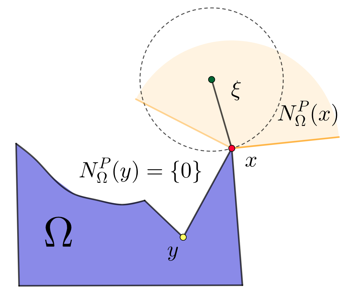
Figure 1: Proximal normal cones

This construction allows us to formulate the notion of uniform prox-regular sets that plays a crucial role in our problem formulations.

Definition 2.1

(Uniform prox-regularity) Let $\Omega$ be a closed subset of $\mathbb{R}^{n}$ and let $\eta>0$. Then $\Omega$ is said to be $\eta$-uniformly prox-regular if for all ${\bf x}\in\mbox{\rm bd}\,\Omega$ and ${\bf v}\in N^{P}_{\Omega}({\bf x})$ with $\|{\bf v}\|=1$ we have

$$B({\bf x}+\eta{\bf v},\eta)\cap\Omega=\emptyset.$$

Equivalently, $\Omega$ is $\eta$-prox-regular if for all ${\bf y}\in\Omega,\;{\bf x}\in\mbox{\rm bd}\,\Omega$, and ${\bf v}\in N^{P}_{\Omega}({\bf x})$ the following inequality holds

$$\left\langle{\bf v},{\bf y}-{\bf x}\right\rangle\leq\dfrac{\|{\bf v}\|}{2\eta}\|{\bf y}-{\bf x}\|^{2}.$$

In other words, $\Omega$ is $\eta$-prox-regular if any external ball with radius smaller than $\eta$ can be rolled around it; see Figure 3 and Figure 3.

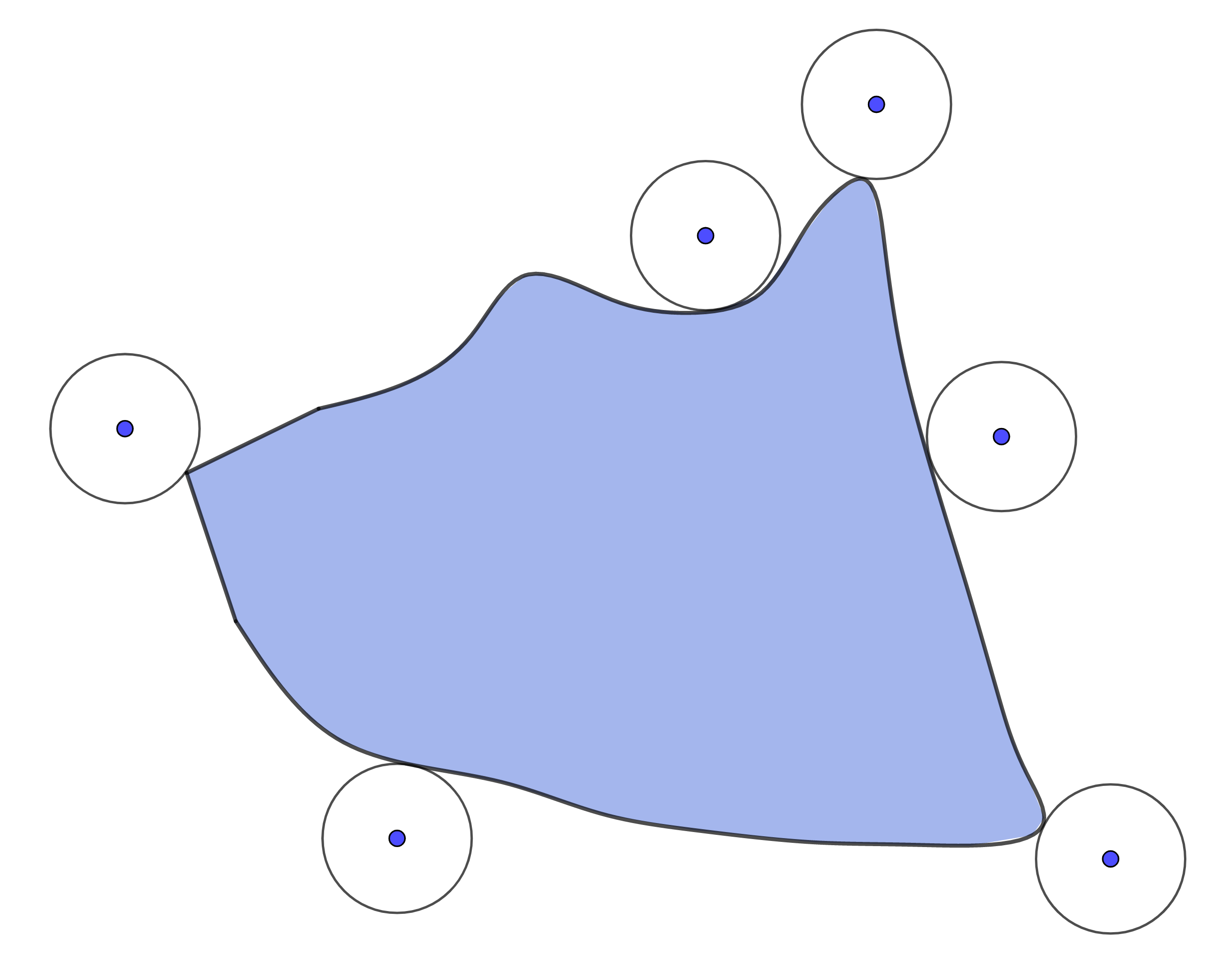
Figure 2: Uniform prox-regular set

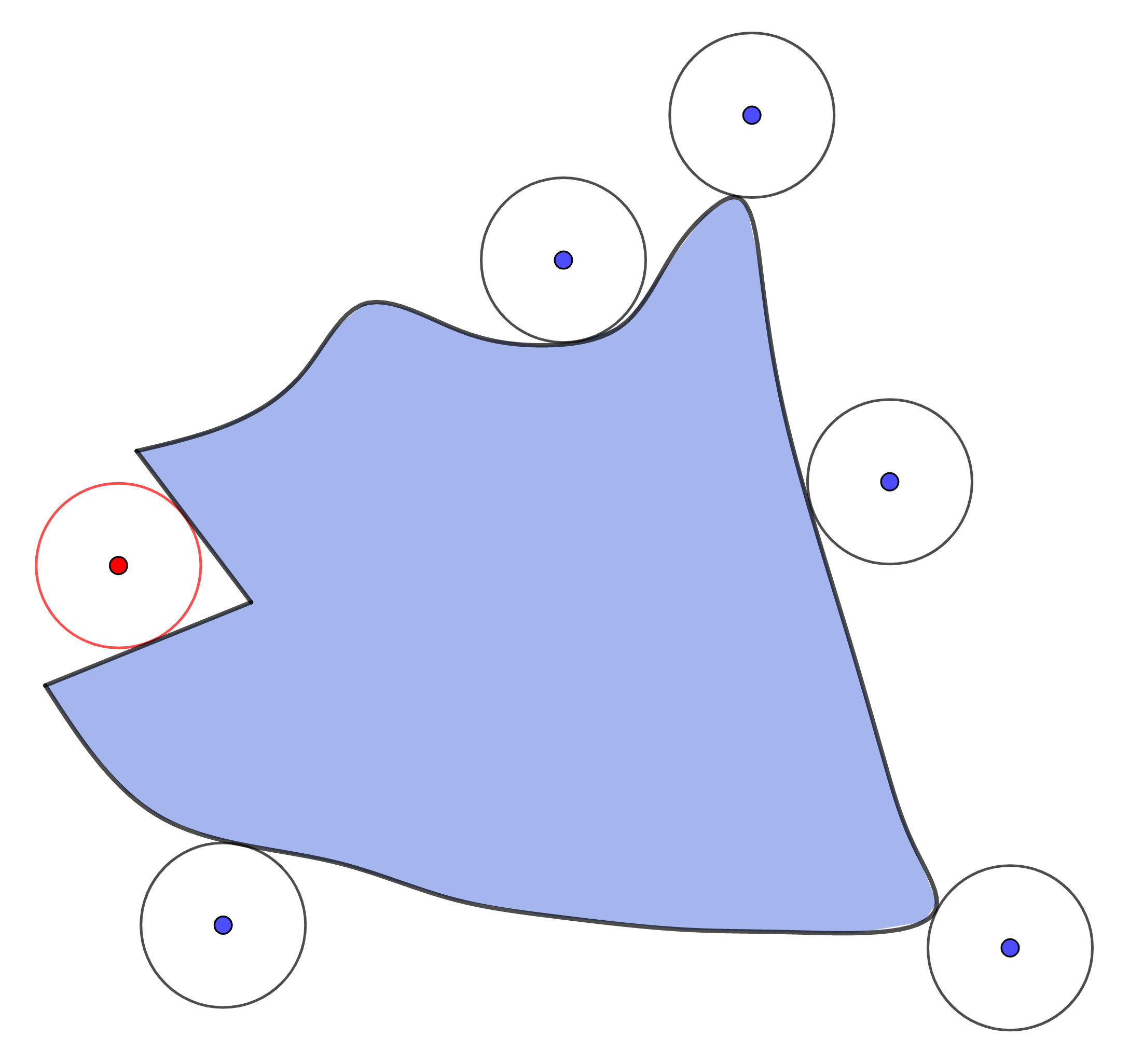
Figure 3: Non uniform prox-regular set

It is worth mentioning that this notion of uniform prox-regularity can be considered as a relaxed version of convexity, i.e., convex sets are $\infty$-uniformly prox-regular. Moreover, this definition ensures that the projection operator $\Pi({\bf x};\Omega)$ onto such a set is well-defined and continuous if $\mbox{\rm dist}\,({\bf x};\Omega)\colon=\inf_{{\bf y}\in\Omega}\|{\bf x}-{\bf y}\|<\eta$. These type of sets are also known as “sets with positive reach” in geometric measure theory; we refer the reader to the excellent survey [20] for numerous results and history of prox-regular sets. In the next sections, we will study the optimal control of several crowd motion models of our own interests.

3 Controlled Motion Models with Single Agent

This section is devoted to the study of the motion models with single agent and several obstacles in general settings. Motivated from [7], consider the motion of an agent identified to an inelastic disk whose center is denoted by ${\bf x}=(x_{1},x_{2})$ and whose radius is $L$ in the given domain $\Omega\in\mathbb{R}^{2}$. Our goal here is find an optimal obstacle-free path $\pi$ of the agent from a start point ${\bf x^{0}}=(x^{0}_{1},x^{0}_{2})$ to a destination ${\bf{\bf x}^{des}}=(x^{des}_{1},x^{des}_{2})$ during the given time interval $[0,T]$ subject to $m$ (static or dynamic) obstacles. To represent the location of the $i$th obstacle, we also use a rigid disk with radius $r_{i}$ whose center is denoted by ${\bf x}^{obs}_{i}=(x^{obs}_{i1},x^{obs}_{i2})$. The agent in this setting can be thought of a robot or a person that moves along the path $\pi$ and is always able to look ahead a distance $L$; for example, to see whether the pathway is clear of debris. This is vitally important especially for safe drivings, the agent should be able to see if there are rocks, limbs, children in the roadway $L$ distance away so that he/she can stop safely or slow down if needed. To reflect this very situation, we introduce the following set of admissible configurations

$$C=\{{\bf x}\in\mathbb{R}^{2}:\;D_{i}({\bf x})\geq 0\;\forall i=1,\ldots,m\}$$ (3.1)

where $D_{i}({\bf x}):=\left\|{{\bf x}}-{\bf x}^{obs}_{i}\right\|-(L+r_{i})$ is the signed distance between the agent and the $i$th obstacle; see Figure 4.

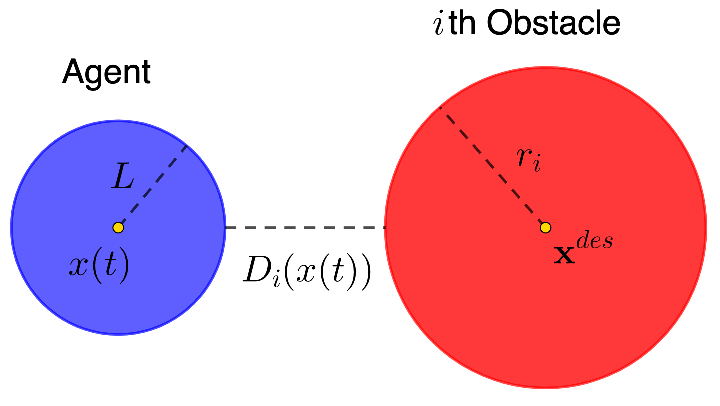
Figure 4: The distance between the agent and the obstacle

In the absence of obstacles, the agent aims to reach the destination using his/her own desired velocity. However, when the agent is in contact with the obstacle in the sense that $D_{i}({{\bf x}})=0$, he/she must adjust the desired velocity to avoid it. In this very case, the desired velocity and the actual velocity do not agree when the obstacle is close enough to the agent. The actual velocity should be selected in such a way that the agent will not collide with the obstacle. In fact, it must belong to the set of admissible velocities $V({\bf x})$ defined as follows

$$V({\bf x})=\{{\bf v}\in\mathbb{R}^{2}:\;D_{i}({\bf x})=0\Rightarrow\left\langle\nabla D_{i}({\bf x}),{\bf v}\right\rangle\geq 0,\forall i=1,\ldots,m\}$$ (3.2)

where $\nabla D_{i}(\cdot)$ denotes the gradient of the function $D_{i}(\cdot)$ and is calculated by

$$\nabla D_{i}({\bf x})=\dfrac{{\bf x}-{{\bf x}^{obs}_{i}}}{\left\|{\bf x}-{{\bf x}^{obs}_{i}}\right\|}.$$

Next let ${\bf U}({\bf x})$ be the desired velocity of the agent assuming that he/she aims to reach the destination using the shortest path. In this case, we have

$${\bf U}({\bf x})=-s\nabla D^{des}({\bf x})$$

where $s$ denotes the speed of the agent and where $D^{des}({\bf x}):=\left\|{\bf x}-{\bf{\bf x}^{des}}\right\|$ represents the distance between the agent and the destination. To ensure the collision free path, the actual velocity denoted by $\dot{\bf x}(t)$ at time $t$ must be selected from the set of admissible velocities $V({\bf x}(t))$ in (3.2). Let us see how this selection can ensure that the agent will not get stuck with the nearby obstacles. Employing the first-order Taylor polynomial for the distance function $D_{i}({\bf x}(t))$ we obtain

$$D_{i}({\bf x}(t+h))=D_{i}({\bf x}(t))+h\left\langle\nabla D_{i}({\bf x}(t)),\dot{\bf x}(t)\right\rangle+o(h)$$

where $h>0$ is a small unit of time. Suppose that the agent is in contact with the obstacle $i$ at time $t$, i.e. $D_{i}({\bf x}(t))=0$. Moreover, since $\dot{\bf x}(t)\in V({\bf x}(t))$, then

$$\left\langle\nabla D_{i}({\bf x}(t)),\dot{\bf x}(t)\right\rangle\geq 0$$

which in turn implies that $D_{i}({\bf x}(t+h))\geq D_{i}({\bf x}(t))=0$. Therefore, the set of admissible configurations in (3.1) ensures that the agent will not collide with the obstacles and the set of admissible velocities in (3.2) offers a guideline to take appropriate actions to avoid the obstacles. Although the actual velocity and the desired velocity of the agent will be no longer the same when the agent is in contact with the obstacles as mentioned above, these two kinds of velocities should not be too much different. To reflect this situation, the actual velocity should be chosen as the closet one to the desired velocity in the following sense

$$\dot{\bf x}(t)=\Pi({\bf U}({\bf x}(t));V({\bf x}(t)))$$ (3.3)

where $\Pi({\bf U}({\bf x}(t));V({\bf x}(t)))$ is defined in (2.8). Using the orthogonal decomposition via the sum of mutually polar cone gives us

$${\bf U}({\bf x}(t)) =\Pi({\bf U}({\bf x}(t));V({\bf x}(t)))+\Pi({\bf U}({\bf x}(t));V^{\ast}({\bf x}(t)))$$

$$=\dot{\bf x}(t)+\Pi({\bf U}({\bf x}(t));V^{\ast}({\bf x}(t)))$$

where $V^{\ast}({\bf x})$ stands for the polar to the admissible velocity set $V({\bf x})$ defined by

$$V^{\ast}({\bf x}):=\left\{{\bf w}:\;\left\langle{\bf w},{\bf v}\right\rangle\leq 0\mbox{ for all }{\bf v}\in V({\bf x})\right\}.$$

It then follows from [39, Proposition 4.1] that

$$V^{\ast}({\bf x})=N^{P}_{C}({\bf x})=\left\{-\lambda_{i}\nabla D_{i}({\bf x})|\;\lambda_{i}\geq 0,D_{i}({\bf x})>0\Rightarrow\lambda_{i}=0\right\}$$

As a consequence, the differential equation (3.3) can be rewritten in the following form of the perturbed sweeping process

$$\dot{\bf x}(t)\in-N_{C}({\bf x}(t))+{\bf U}({\bf x}(t))$$

which is a special case of (1.1). Consider the following optimal control problem, denoted by $(P)$.

$$\mbox{minimize}\;\;J[{\bf x},a]=\frac{1}{2}\left\|{\bf x}(T)-{\bf x}^{des}\right\|^{2}+\frac{\tau}{2}\int^{T}_{0}\left\|a(t)\right\|^{2}dt$$ (3.4)

over the control functions $a(\cdot)\in L^{2}([0,T];\mathbb{R})$ and the corresponding trajectory ${\bf x}(\cdot)\in W^{1,2}([0,T];\mathbb{R}^{2})$ of the nonconvex sweeping process

$$\begin{cases}\dot{\bf x}(t)\in-N_{C}({\bf x}(t))+{\bf U}({\bf x}(t),a(t))\;\;\mbox{a.e.}\;\;t\in[0,T],\\ {\bf U}({\bf x},a):=-sa\nabla D^{des}({\bf x})=-sa\dfrac{{\bf x}-{\bf x}^{des}}{\left\|{\bf x}-{\bf x}^{des}\right\|},\\ {\bf x}(0)={\bf x}_{0}\in C\end{cases}$$ (3.5)

where the set $C$ is given in (3.1), where ${\bf U}({\bf x},a)$ denotes the controlled desired velocity, and where $\tau>0$ is a given constant. The meaning of the cost functional in (3.4) is minimizing the distance of the agent to the destination together with the minimum energy of feasible controls $a(\cdot)$ used to adjust the desired velocity. Let us first consider the control problem with single obstacle ($m=1$) and recall the corresponding set of necessary conditions derived in [7].

3.1 Necessary Optimality Conditions

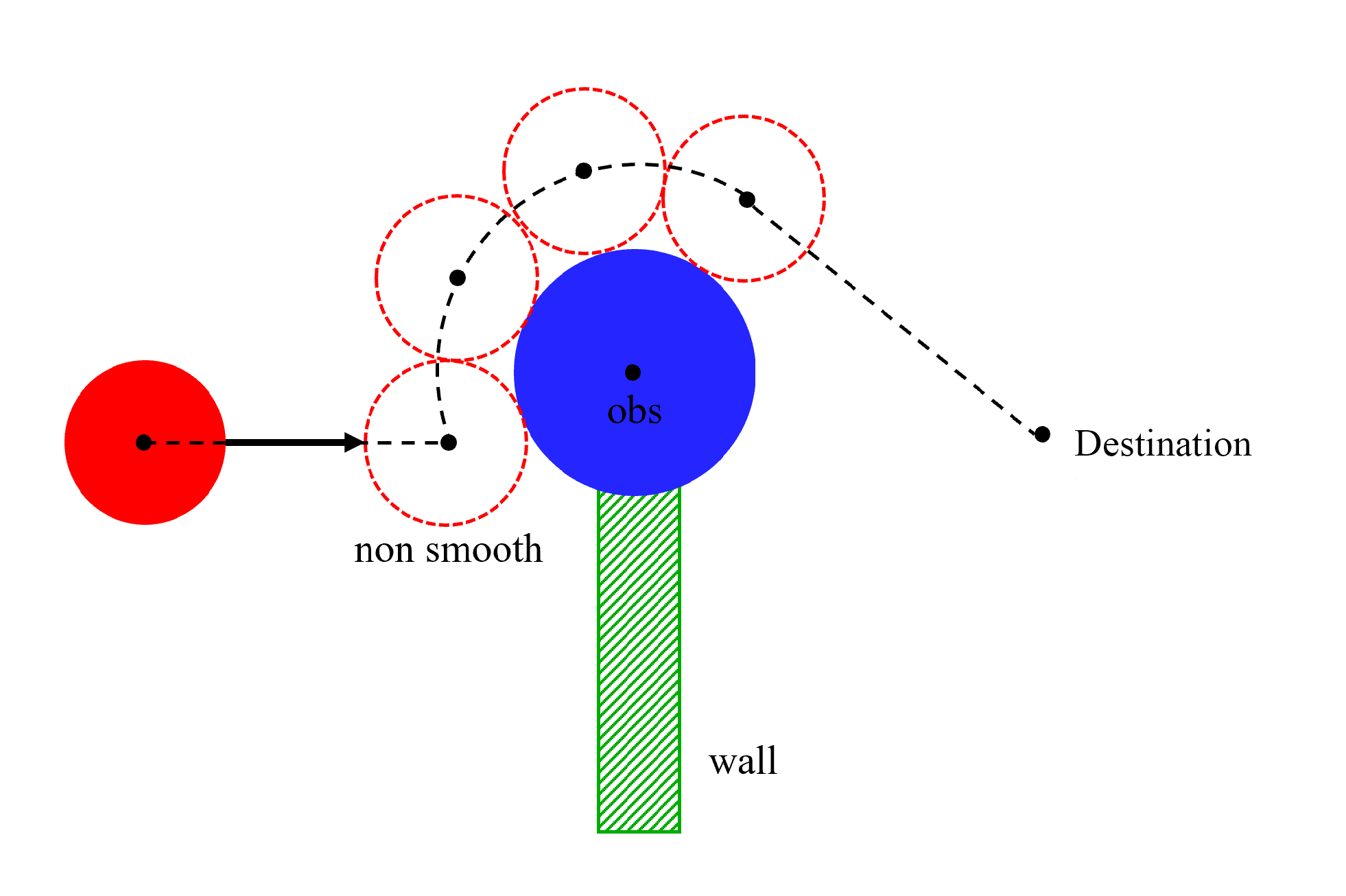
Figure 5: The controlled crowd motion with single agent and single obstacle

Theorem 3.1

(Necessary optimality conditions for optimization of controlled crowd motions with obstacles) Let $(\overline{\bf x}(\cdot),\overline{a}(\cdot))\in W^{2,\infty}([0,T];\mathbb{R}^{2}\times\mathbb{R})$ be a strong local minimizer of the crowd motion problem in (3.4). There exist some dual elements $\lambda\geq 0,\;\eta(\cdot)\in L^{2}([0,T];\mathbb{R}_{+})$ well-defined at $t=T$ ${\bf w}(\cdot)=({\bf w}^{x}(\cdot),{\bf w}^{a}(\cdot))\in L^{2}([0,T];\mathbb{R}^{2}\times\mathbb{R})$, ${\bf v}(\cdot)=({\bf v}^{x}(\cdot),{\bf v}^{a}(\cdot))\in L^{2}([0,T];\mathbb{R}^{2}\times\mathbb{R})$, an absolutely continuous vector function ${\bf p}(\cdot)=({\bf p}^{x}(\cdot),{\bf p}^{a}(\cdot))\in W^{1,2}([0,T];\mathbb{R}^{2})$, a measure $\gamma\in C^{*}([0,T];\mathbb{R}^{2})$, and a vector function ${\bf q}(\cdot)=({\bf q}^{x}(\cdot),{\bf q}^{a}(\cdot)):[0,T]\to\mathbb{R}^{2}\times\mathbb{R}$ of bounded variation on $[0,T]$ such that the following conditions are satisfied:

1. ${\bf w}(t)=(0,\overline{a}(t)),\;\;{\bf v}(t)=(0,0)$ for a.e. $t\in[0,T]$;

2. $\dot{\overline{\bf x}}(t)=-s\overline{a}(t)d\left(\overline{\bf x}(t),{\bf x}^{des}\right)-\eta(t)d\left({\bf x}^{obs},\overline{\bf x}(t)\right)$ for a.e. $t\in[0,T]$, where $d({\bf x},{\bf y}):=\dfrac{{\bf x}-{\bf y}}{\left\|{\bf x}-{\bf y}\right\|}$;

3. $\left\|{\bf x}(t)-{\bf x}^{obs}\right\|>L+r\Longrightarrow\eta(t)=0$;

4. $\eta(t)>0\Longrightarrow\left\langle{\bf q}^{x}(t),{\bf x}^{obs}-\overline{\bf x}(t)\right\rangle=0$ for a.e. $t\in[0,T]$;

5. $\dot{\bf p}(t)=\bigg{(}0,\lambda\overline{a}(t)-s\big{[}\left\langle{\bf q}^{x}(t),d(\overline{\bf x}(t),{\bf x}^{des})\right\rangle\big{]}\bigg{)}$;

6. ${\bf q}^{x}(t)={\bf p}^{x}(t)+\gamma([t,T])$ for a.e. $t\in[0,T]$;

7. ${\bf q}^{a}(t)={\bf p}^{a}(t)=0$ for a.e. $t\in[0,T]$;

8. ${\bf p}^{x}(T)+\lambda\overline{(}{\bf x}(T)-{\bf x}^{des})=-\eta(T)d({\bf x}^{obs},\overline{\bf x}(T))$;

9. ${\bf p}^{a}(T)=0$;

10. $\lambda+\|{\bf p}^{x}(T)\|>0$.

Proof. To justify our claim, we elaborate the arguments that are similar to those in the proof of [13, Theorem 3.1] for the following data sets of the model under consideration:

$$\begin{cases}g({\bf x})\colon=\|{\bf x}-{\bf x}^{obs}\|-(L+r),\\ V\colon=\left\{{\bf x}\in\mathbb{R}|\;\|{\bf x}-{\bf x}^{obs}\|>\frac{1}{2}(L+r)\right\}.\end{cases}$$

Then $g$ is convex, belongs to the space $\mathcal{C}^{2}(V)$ with the above open set $V$, and satisfies estimate (2.3) in [13] with $c\colon=\dfrac{L+r}{\sqrt{2}}$. Moreover, it is obvious that

$$\|\nabla g({\bf x})\|=1\;\mbox{ and }\left\|\nabla^{2}g({\bf x})\right\|\leq\dfrac{2}{L+r}\mbox{ for all }{\bf x}\in V$$

and hence the inequalities (2.4) and (2.5) in [13] hold, which completes the proof of the theorem. $\hfill\quad\square$

The authors in [7] considered a particular numerical example with the given data illustrating the above necessary optimality conditions and solved the problem successfully. In what follows, we consider a general numerical framework with arbitrary data which can be described as follows:

• The ending time $T$ is given.

• The initial position of the agent is ${\bf x}^{0}=(x^{0}_{1},x^{0}_{2})$.

• The position of the agent is ${\bf x}(t)=(x_{1}(t),x_{2}(t))$ assuming that he/she is identified to the disk whose center is ${\bf x}(t)$ and whose radius is $L>0$.

• The obstacle is located at the rigid disk with radius $r$ whose center is ${\bf x}^{obs}=(x_{1}^{obs},x_{2}^{obs})$.

• The destination is ${\bf x}^{des}=(x_{1}^{des},x_{2}^{des})$.

• The (uncontrolled) constant speed of the agent during $[0,T]$ is $s=\dfrac{\sqrt{(x^{des}_{1}-x^{0}_{1})^{2}+(x^{des}_{2}-x^{0}_{2})^{2}}}{T}$.

• The running cost presents the energy that the agent used to adjust his/her speed and is given by $\ell=\dfrac{a^{2}}{2}$.

• The terminal cost is $\varphi(x)=\frac{1}{2}\sqrt{(x^{des}_{1}-x^{0}_{1})^{2}+(x^{des}_{2}-x^{0}_{2})^{2}}$.

Our goal here is to find the best control strategies for which the agent is able to get close to the target while avoiding the obstacle using the minimum energy. Employing the necessary optimality conditions in Theorem 3.1 gives us the dual elements satisfying all conditions from (1) to (10). To reduce the complexity of the problem, the control function $\overline{a}(t)$ is assumed to be constant during $[0,T]$; that is $\overline{a}(t)\equiv\overline{a}$ for all $t\in[0,T]$. Recall that desired velocity of the agent is given by

$${\bf U}(\overline{\bf x}(t),\overline{a})=-s\overline{a}\dfrac{\overline{\bf x}(t)-{\bf x}^{des}}{\left\|\overline{\bf x}(t)-{\bf x}^{des}\right\|}$$

pointing in the direction towards the target, while the control $a$ is used to adjust the speed of the agent. It is not hard to see that $\overline{a}>0$ in this setting. When the agent is nearby the obstacle, he/she must take it into account on the way to the target. So his/her actual velocity described by (2) has the following representation

$$\dot{\overline{\bf x}}(t)=-s\overline{a}\dfrac{\overline{\bf x}(t)-{\bf x}^{des}}{\left\|\overline{\bf x}(t)-{\bf x}^{des}\right\|}-\eta(t)\dfrac{{\bf x}^{obs}-\overline{\bf x}(t)}{\|{\bf x}^{obs}-\overline{\bf x}(t)\|}$$ (3.6)

for a.e. $t\in[0,T]$, where the second term in the right hand side is generated from the proximal normal cone $N^{P}_{C}({\bf x}(t))$. Let $t_{f}$ and $t_{l}$ be the first time that the agent is in contact with the obstacle and the first time that he/she leaves the obstacle respectively. The agent would behave differently during the time interval $[0,T]$ depending on his/her contact with the obstacle. Before the contact time $t_{f}$, the agent heads towards the target with the velocity

$$\dot{\overline{\bf x}}(t)={\bf U}(\overline{\bf x}(t),\overline{a})=-s\overline{a}\dfrac{\overline{\bf x}(t)-{\bf x}^{des}}{\left\|\overline{\bf x}(t)-{\bf x}^{des}\right\|}$$

for all $t\in[0,t_{f})$, i.e. the actual and desired velocities are identical.

(a) The behavior of the agent when he/she is first in contact with the obstacle: In this case we have $\|{\bf x}^{obs}-\overline{\bf x}(t)\|=L+r$ which hence implies that

$$\left\langle\overline{\bf x}(t)-{\bf x}^{obs},\overline{\bf x}(t)-{\bf x}^{obs}\right\rangle=(L+r)^{2}$$

for all $t\in[t_{f},t_{l}]$. Differentiating both sides of the above equation with respect to $t$ gives us

$$\left\langle\dot{\overline{\bf x}}(t),\overline{\bf x}(t)-{\bf x}^{obs}\right\rangle=0$$ (3.7)

for a.e. $t\in[t_{f},t_{l}]$. Combining this with the representation of $\dot{\overline{\bf x}}(t)$ in (3.6) we obtain

$$\left\langle-s\overline{a}\dfrac{\overline{\bf x}(t)-{\bf x}^{des}}{\left\|\overline{\bf x}(t)-{\bf x}^{des}\right\|}-\eta(t)\dfrac{{\bf x}^{obs}-\overline{\bf x}(t)}{\|{\bf x}^{obs}-\overline{\bf x}(t)\|},\overline{\bf x}(t)-{\bf x}^{obs}\right\rangle=0$$

and thus get the useful information for the scalar function $\eta(t)$ as follows

$$\eta(t)=s\overline{a}\left\langle\dfrac{\overline{\bf x}(t)-{\bf x}^{des}}{\left\|\overline{\bf x}(t)-{\bf x}^{des}\right\|},\dfrac{\overline{\bf x}(t)-{\bf x}^{obs}}{\left\|\overline{\bf x}(t)-{\bf x}^{obs}\right\|}\right\rangle.$$ (3.8)

This tells us that the behavior of $\eta(\cdot)$ heavily depends on the position of the agent with respect to the obstacle and the destination. Note that $\eta(t)$ will achieve its maximum value when two unit vectors $\dfrac{\overline{\bf x}(t)-{\bf x}^{des}}{\left\|\overline{\bf x}(t)-{\bf x}^{des}\right\|}$ and $\dfrac{\overline{\bf x}(t)-{\bf x}^{obs}}{\left\|\overline{\bf x}(t)-{\bf x}^{obs}\right\|}$ point in the same direction; that is $\overline{x}(t),{\bf x}^{obs}$, and ${\bf x}^{des}$ are collinear; see Figure 7. In this very situation the vector $\eta(t)\dfrac{\overline{\bf x}(t)-{\bf x}^{obs}}{\left\|\overline{\bf x}(t)-{\bf x}^{obs}\right\|}$ will have the maximum effect pushing the agent away from the obstacle which is reflected in (3.6). On the other hand, it follows from (5) and (7) that

$$\lambda\overline{a}=s\left\langle{\bf q}^{x}(t),\dfrac{\overline{\bf x}(t)-{\bf x}^{des}}{\left\|\overline{\bf x}(t)-{\bf x}^{des}\right\|}\right\rangle$$

and thus

$$\left\langle{\bf q}^{x}(t),\dot{\overline{\bf x}}(t)\right\rangle =-s\overline{a}\left\langle{\bf q}^{x}(t),\dfrac{\overline{\bf x}(t)-{\bf x}^{des}}{\left\|\overline{\bf x}(t)-{\bf x}^{des}\right\|}\right\rangle-\eta(t)\left\langle{\bf q}^{x}(t),\dfrac{{\bf x}^{obs}-\overline{\bf x}(t)}{\|{\bf x}^{obs}-\overline{\bf x}(t)\|}\right\rangle$$

$$=-\lambda\overline{a}^{2}-\eta(t)\left\langle{\bf q}^{x}(t),\dfrac{{\bf x}^{obs}-\overline{\bf x}(t)}{\|{\bf x}^{obs}-\overline{\bf x}(t)\|}\right\rangle$$

for a.e. $t\in[0,T]$.

$\bullet$ If $\eta(t)=0$, $\left\langle{\bf q}^{x}(t),\dot{\overline{\bf x}}(t)\right\rangle=-\lambda\overline{a}^{2}$.

$\bullet$ If $\eta(t)>0$, using (4) also gives us $\left\langle{\bf q}^{x}(t),\dot{\overline{\bf x}}(t)\right\rangle=-\lambda\overline{a}^{2}$.

In general, we have

$$\left\langle{\bf q}^{x}(t),\dot{\overline{\bf x}}(t)\right\rangle=-\lambda\overline{a}^{2}<0$$ (3.9)

for a.e. $t\in[0,T]$. Let us next track the positions of the agent during the contact time interval $[t_{f},t_{l}]$.

(b) The positions of the agent during the contact time interval $[t_{f},t_{l}]$: Once the agent is in contact with the obstacle, he/she would stay on the circle centered at ${\bf x}^{obs}=(x^{obs}_{1},x^{obs}_{2})$ with radius $L+r$ and would leave the obstacle at $t=t_{l}$. In this case it makes a perfect sense to assume that $\eta(t)>0$, that is the normal cone $N_{C}({\bf x}(t))$ is activated (or nontrivial) on $[t_{f},t_{l})$. Then using condition (4) and (3.7) we deduce that two vectors ${\bf q}^{x}(t)$ and $\dot{\overline{\bf x}}(t)$ are parallel in $\mathbb{R}^{2}$, i.e.,

$${\bf q}^{x}(t)=m(t)\dot{\overline{\bf x}}(t)$$ (3.10)

for some scalar function $m(\cdot)$. Combining this with (3.9) we obtain that

$$m(t)\|\dot{\overline{\bf x}}(t)\|^{2}=-\lambda\overline{a}^{2}$$

and that $m(t)<0$ showing that ${\bf q}^{x}(t)$ points in the opposite direction of the velocity $\dot{\overline{\bf x}}(t)$. For simplicity we assume that the agent only switches the speed at the time he/she first is in contact with the obstacle and at the time he/she leaves it. This ensures that $\|\dot{\overline{\bf x}}(\cdot)\|$ is piecewise constant on $[0,T]$ and hence $m(\cdot)$ is constant on $[t_{f},t_{l}),$ i.e. $m(t)\equiv m$ on $[t_{f},t_{l})$. Rewrite the above equation we get

$$\|\dot{\overline{\bf x}}(t)\|=K|\overline{a}|$$

where $K:=\sqrt{-\dfrac{\lambda}{m}}$. For convenience, we select $\lambda=-m$ and thus

$$\|\dot{\overline{\bf x}}(t)\|=|\overline{a}|$$ (3.11)

for a.e. $t\in[t_{f},t_{l}]$. Hence, the distance traveled during the contact time interval $[t_{f},t_{l}]$ can be computed by

$$\int^{t_{l}}_{t_{f}}\|\dot{\overline{\bf x}}(t)\|dt=(t_{l}-t_{f})|\overline{a}|.$$ (3.12)

We next track the position of the agent ${\bf x}(t_{l})$ when he/she leaves the obstacle. In this case two vectors $\dfrac{\overline{\bf x}(t)-{\bf x}^{des}}{\left\|\overline{\bf x}(t)-{\bf x}^{des}\right\|}$ and $\dfrac{\overline{\bf x}(t)-{\bf x}^{obs}}{\left\|\overline{\bf x}(t)-{\bf x}^{obs}\right\|}$ are orthogonal, that is $\eta(t)=0$ due to (3.8). In fact, when the agent first is in contact with the obstacle, he/she will move in either one of two directions to reach the destination (see the figure). Thus, there are two possible locations of ${\bf x}(t_{l})$ and we should select the one that has a shorter traveled distance from ${\bf x}(t_{f})$. The coordinates of ${\bf x}(t_{l})=(x_{1}(t_{l}),x_{2}(t_{l}))$ can be determined by finding the intersection of the circle centered at ${\bf x}^{obs}$ with radius $L+r$ and the circle centered at $\frac{1}{2}({\bf x}^{obs}+{\bf x}^{des})$ with radius $\frac{1}{2}\sqrt{(x^{des}_{1}-x^{obs}_{1})^{2}+(x^{des}_{2}-x^{obs}_{2})^{2}}$. Hence, $x_{1}(t_{l})$ and $x_{2}(t_{l})$ satisfy the following system of equations

$$\begin{cases}\left(x_{1}-\dfrac{x^{obs}_{1}+x^{des}_{1}}{2}\right)^{2}+\left(x_{2}-\dfrac{x^{obs}_{2}+x^{des}_{2}}{2}\right)^{2}=\dfrac{(x^{des}_{1}-x^{obs}_{1})^{2}+(x^{des}_{2}-x^{obs}_{2})^{2}}{4}\\[8.61108pt] \left(x_{1}-x^{obs}_{1}\right)^{2}+\left(x_{2}-x^{obs}_{2}\right)^{2}=(L+r)^{2}\end{cases}$$ (3.13)

which is equivalent to

$$\begin{cases}\left(x_{1}-x^{obs}_{1}\right)^{2}+\left(x_{2}-x^{obs}_{2}\right)^{2}=(L+r)^{2}\\[8.61108pt] \left(x^{obs}_{1}-x^{des}_{1}\right)\left(x_{1}-\dfrac{x^{des}_{1}+3x^{obs}_{1}}{4}\right)+\left(x^{obs}_{2}-x^{des}_{2}\right)\left(x_{2}-\dfrac{x^{des}_{2}+3x^{obs}_{2}}{4}\right)\\[8.61108pt] =\dfrac{(x^{des}_{1}-x^{obs}_{1})^{2}+(x^{des}_{2}-x^{obs}_{2})^{2}}{4}-(L+r)^{2}.\end{cases}$$

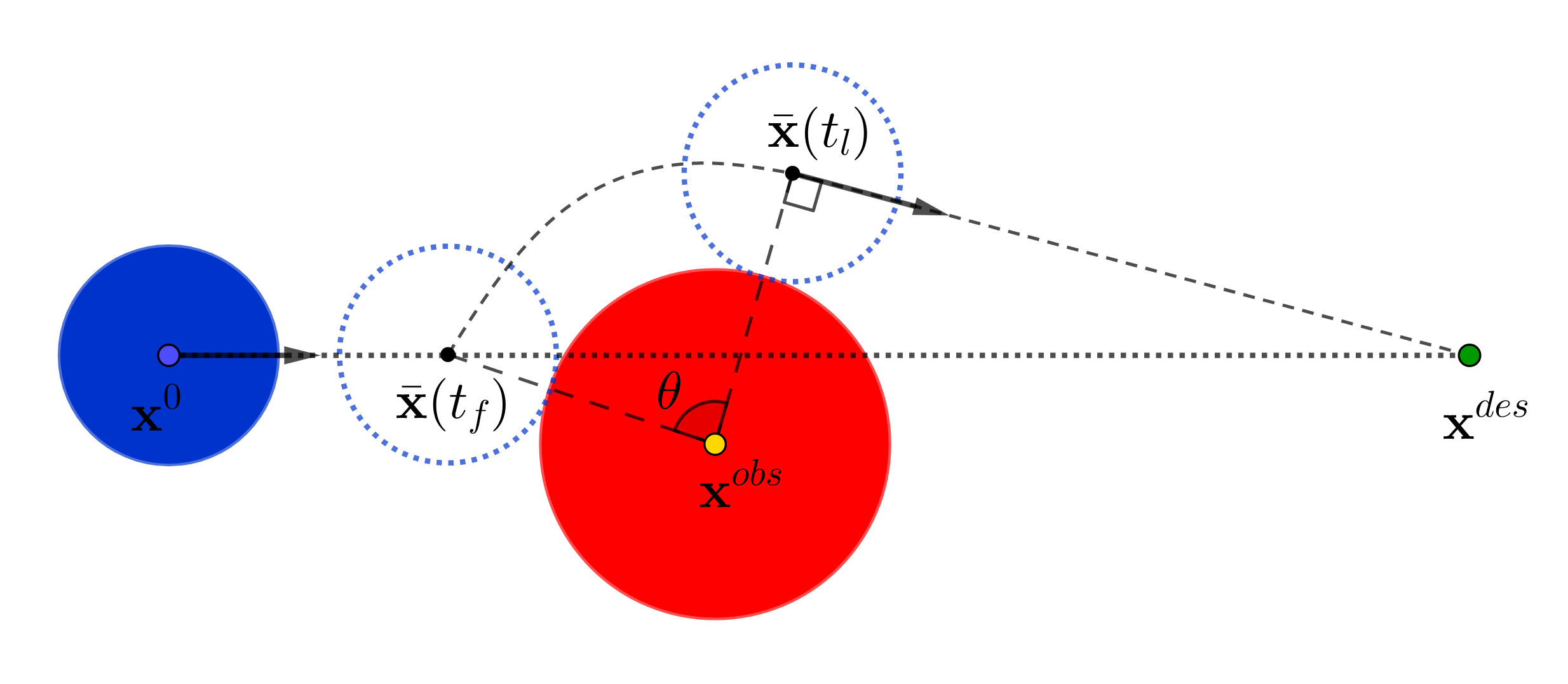
Figure 6: The controlled crowd motion with single agent and single obstacle

Let $\theta$ be the angle between two vectors ${\bf x}(t_{f})-{\bf x}^{obs}$ and ${\bf x}(t_{l})-{\bf x}^{obs}$. Then

$$\theta=\cos^{-1}\left(\left\langle\dfrac{\overline{\bf x}(t_{f})-{\bf x}^{obs}}{\|\overline{\bf x}(t_{f})-{\bf x}^{obs}\|},\dfrac{\overline{\bf x}(t_{l})-{\bf x}^{obs}}{\|\overline{\bf x}(t_{l})-{\bf x}^{obs}\|}\right\rangle\right).$$ (3.14)

When the components of $\overline{\bf x}(t_{l})=(\overline{x}_{1}(t_{l}),\overline{x}_{2}(t_{l}))$ are determined by solving the system of equations in (3.13), we are able to find the value of $\theta$ using (3.14). In fact, this system of equations has two possible solutions which hence gives us two corresponding values of $\theta$, say $\theta_{1}$ and $\theta_{2}$. Then we can select $\theta$ as $\theta=\min\{\theta_{1},\theta_{2}\}$. In other words, the coordinates of $\overline{\bf x}(t_{l})$ are the solutions of the system (3.13) that minimize $\left\|\overline{\bf x}(t_{l})-\overline{\bf x}(t_{f})\right\|$.

In fact, the control $\overline{a}$ needs to take sufficiently large enough value to support the agent, at least, to exceed the position ${\bf x}(t_{l})$, i.e., $t_{l}\leq T$. The distance of the agent travels from $t=t_{f}$ to $t=t_{l}$ can be found as follows

$$\int^{t_{l}}_{t_{f}}\|\dot{\overline{\bf x}}(t)\|\;dt=\dfrac{\pi\theta(r+L)}{180}.$$

Combining this with (3.12) gives us

$$(t_{l}-t_{f})|\overline{a}|=\dfrac{\pi\theta(r+L)}{180}$$

which hence implies that

$$t_{l}=\dfrac{\pi\theta(r+L)}{180|\overline{a}|}+t_{f}.$$ (3.15)

Note that $t_{f}=\dfrac{\|\overline{\bf x}(t_{f})-{\bf x^{0}}\|}{s|\overline{a}|}.$ Therefore, the assumption that $t_{l}\leq T$ yields

$$\dfrac{\|\overline{\bf x}(t_{f})-{\bf x^{0}}\|}{s|\overline{a}|}+\dfrac{\pi\theta(r+L)}{180|\overline{a}|}\leq T.$$

Equivalently,

$$|\overline{a}|\geq\dfrac{1}{T}\left(\dfrac{\|\overline{\bf x}(t_{f})-{\bf x^{0}}\|}{s}+\dfrac{\pi\theta(r+L)}{180}\right).$$ (3.16)

The distances the agent travels during the contact time $[t_{f},t_{l}]$ and after the contact time: In fact the distance of the agent travels from $t=t_{f}$ to $t=t_{l}$ can be found as follows

$$\int^{t_{l}}_{t_{f}}\|\dot{\overline{\bf x}}(t)\|\;dt=\dfrac{\pi\theta(r+L)}{180^{\circ}}.$$

Combining this with (3.12) gives us

$$(t_{l}-t_{f})|\overline{a}|=\dfrac{\pi\theta(r+L)}{180}$$

which hence implies that

$$t_{l}=\dfrac{\pi\theta(r+L)}{180|\overline{a}|}+t_{f}.$$

We next compute the distance that the agent traveled from $t=0$ to $t=t_{f}$. To proceed we first determine the coordinates of ${\bf x}(t_{f})$ whose representation is given as follows

$$\overline{\bf x}(t_{f})=(1-\mu){\bf x}^{0}+\mu{\bf x}^{des},$$

where $\mu\in[0,1]$. At $t=t_{f}$, the agent is contact with the obstacle, so

$$\left\|\overline{\bf x}(t_{f})-{\bf x}^{obs}\right\|=r+L.$$

In other words, $\mu$ is the solution of the equation

$$\left\|\left[(1-\mu){\bf x}^{0}+\mu{\bf x}^{des}\right]-{\bf x}^{obs}\right\|=r+L$$ (3.17)

that minimizes $d(\mu):=\left\|\left[(1-\mu){\bf x}^{0}+\mu{\bf x}^{des}\right]-{\bf x}^{0}\right\|=\mu\left\|{\bf x}^{des}-{\bf x}^{0}\right\|$. Then the time $t=t_{f}$ can be computed by

$$t_{f}=\dfrac{d(\mu)}{s|\overline{a}|}$$

which leads us in turn to

$$t_{l}=\dfrac{\pi\theta(r+L)}{180\overline{a}}+\dfrac{d(\mu)}{s|\overline{a}|}.$$

In addition, the distance that the agent travels from $t=t_{l}$ to $t=T$ (the ending time) is

$$\left\|\overline{\bf x}(t_{l})-{\bf x}^{des}\right\|-\left\|\overline{\bf x}(T)-{\bf x}^{des}\right\|,$$

which can also be found by multiplying the travel time $(T-t_{l})$ by the constant speed $s|\overline{a}|$. As a result, we have

$$(T-t_{l})s|\overline{a}|=\left\|{\bf x}(t_{l})-{\bf x}^{des}\right\|-\left\|{\bf x}(T)-{\bf x}^{des}\right\|$$

and hence obtain

$$\left\|\overline{\bf x}(T)-{\bf x}^{des}\right\|=\left\|\overline{\bf x}(t_{l})-{\bf x}^{des}\right\|-(T-t_{l})s|\overline{a}|.$$

Therefore, the cost functional can be written in the following form

$$J =\frac{1}{2}\left[\left\|\overline{\bf x}(t_{l})-{\bf x}^{des}\right\|-(T-t_{l})s|\overline{a}|\right]^{2}+\dfrac{\tau T}{2}\overline{a}^{2}$$ (3.18)

$$=\frac{1}{2}\left[\left\|\overline{\bf x}(t_{l})-{\bf x}^{des}\right\|-\left(T-\dfrac{\pi\theta(r+L)}{180|\overline{a}|}-\dfrac{d(\mu)}{s|\overline{a}|}\right)s|\overline{a}|\right]^{2}+\dfrac{\tau T}{2}\overline{a}^{2}$$

$$=\frac{1}{2}\left[\left\|\overline{\bf x}(t_{l})-{\bf x}^{des}\right\|-\left(T|\overline{a}|-\dfrac{\pi\theta(r+L)}{180}-\dfrac{d(\mu)}{s}\right)s\right]^{2}+\dfrac{\tau T}{2}\overline{a}^{2}.$$

Minimizing this cost functional with respect to $\overline{a}$ gives us an optimal control $\overline{a}$. Our work can be summarized in Algorithm 1.

Our next task is to compute the corresponding trajectory. We first consider the cases when the agent is not in contact with the obstacle, i.e. $t\notin[t_{f},t_{l}]$. In such cases, the actual velocity and desired velocity are identical, that is

$$\dot{\overline{\bf x}}(t) ={\bf U}(\overline{\bf x}(t),\overline{a})=-s\overline{a}\dfrac{\overline{\bf x}(t)-{\bf x}^{des}}{\left\|\overline{\bf x}(t)-{\bf x}^{des}\right\|}$$

$$=\begin{cases}-s\overline{a}(\cos\alpha_{1},\sin\alpha_{1})&\mbox{ if }t<t_{f}\\ -s\overline{a}(\cos\alpha_{2},\sin\alpha_{2})&\mbox{ if }t>t_{l}\end{cases}$$

where $\alpha_{1}=\angle({\bf x}^{0}-{\bf x}^{des},\bf i)$ and $\alpha_{2}=\angle({\bf x}(t_{l})-{\bf x}^{des},\bf i)$. As a consequence,

$$\overline{\bf x}(t)=\begin{cases}{\bf x}^{0}-s\overline{a}t(\cos\alpha_{1},t\sin\alpha_{1})&\mbox{ if }t<t_{f}\\ \overline{\bf x}(t_{l})-s\overline{a}(t-t_{l})(\cos\alpha_{2},t\sin\alpha_{2})&\mbox{ if }t>t_{l}.\end{cases}$$

For all $t\in[t_{f},t_{l}]$, let $\theta_{t}$ be the angle between ${\bf x}(t_{f})-{\bf x}^{obs}$ and ${\bf x}(t)-{\bf x}^{obs}$. It then follows that

$$\theta_{t}=\dfrac{(t-t_{f})|\overline{a}|}{r+L}.$$

Denote $\alpha=\angle(\overline{\bf x}(t_{f})-{\bf x}^{obs},{\bf i}),\;A=\left[\begin{array}[]{c c}\cos(-\alpha)&-\sin(-\alpha)\\ \sin(-\alpha)&\cos(-\alpha)\end{array}\right],$ and ${\bf y}=(\overline{y}_{1},\overline{y}_{2})=(\overline{\bf x}(t_{l})-{\bf x}^{obs})A^{T}$. The trajectory of the agent when he or she is in contact with the obstacle can be computed as follows

$$\overline{\bf x}(t)=\begin{cases}{\bf x}^{obs}+(\overline{\bf x}(t_{f})-{\bf x}^{obs})\left[\begin{array}[]{c c}\cos(\theta_{t})&\sin(\theta_{t})\\ -\sin(\theta_{t})&\cos(\theta_{t})\end{array}\right]\qquad&\text{ if }\overline{y}_{2}\geq 0,\\ &\\ {\bf x}^{obs}+(\overline{\bf x}(t_{f})-{\bf x}^{obs})\left[\begin{array}[]{c c}\cos(-\theta_{t})&\sin(-\theta_{t})\\ -\sin(-\theta_{t})&\cos(-\theta_{t})\end{array}\right]&\text{ otherwise,}\end{cases}$$

for $t\in[t_{f},t_{l}]$. During the contact time, the normal cone $N_{C}(\overline{\bf x}(t))$ is activated with $\eta(t)$ which is given by (3.8) and hence can be written in the following form

$$\eta(t)=\left\langle{\bf U}(\overline{\bf x}(t),\overline{a}),\dfrac{{\bf x}^{obs}-\overline{\bf x}(t)}{\|{\bf x}^{obs}-\overline{\bf x}(t)\|}\right\rangle.$$

It is interesting to see that $\eta(t)$ keeps track the connection between the desired velocity and the agent’s position relative to the obstacle.

3.2 Illustrative Examples

In this section, we present several examples to illustrate some characteristic features of the necessary optimality conditions derived in Theorem 3.1. These examples are solved using Algorithm 1 and the corresponding Python code.

Example 3.2

Let us first consider an example in [7] with the following data:

$$\begin{cases}T=6,\;{\bf x}_{0}=(0,48),\;{\bf x}^{obs}=(0,24),\;{\bf x}^{des}=(0,0),\\ s=\frac{48}{6}=8,\;r=L=3.\end{cases}$$

In this case the positions of the agent, the obstacle, and the destination are collinear (see Figure 7).

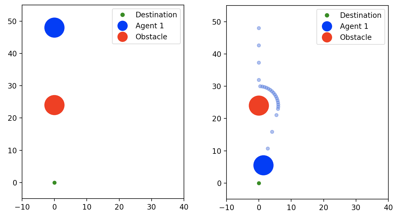
Figure 7: Illustration for Example 3.2 at $t=0$ and $t=T$

The performances of the agent are recorded in the following table with various values of $\tau>0$.

$\tau$	$\overline{a}$	$t_{f}$	$t_{l}$	$J[{\overline{\bf x}},\overline{a}]$
1.0	2.675632	0.840923	4.929998	21.532945
2.0	2.668700	0.843107	4.942803	42.954320
3.0	2.661804	0.845291	4.955609	64.264990
4.0	2.654944	0.847476	4.968414	85.465812
5.0	2.648119	0.849660	4.981219	106.557632
6.0	2.641329	0.851844	4.994024	127.541289
7.0	2.634573	0.854028	5.006829	148.417612
8.0	2.627853	0.856212	5.019635	169.187424
9.0	2.621166	0.858397	5.032440	189.851537
10.0	2.614513	0.860581	5.045245	210.410756

Note that the results shown in the above table are slightly different from the ones in [7]. In fact the first time the agent is in contact with the obstacle, denoted by $t_{1}$ in [7] which is $t_{f}$ in this paper, was miscalculated. It should be $t_{1}=\dfrac{24-6}{8|\overline{a}|}=\dfrac{18}{8\overline{a}}$, not $\dfrac{24}{8\overline{a}}$ as in [7].

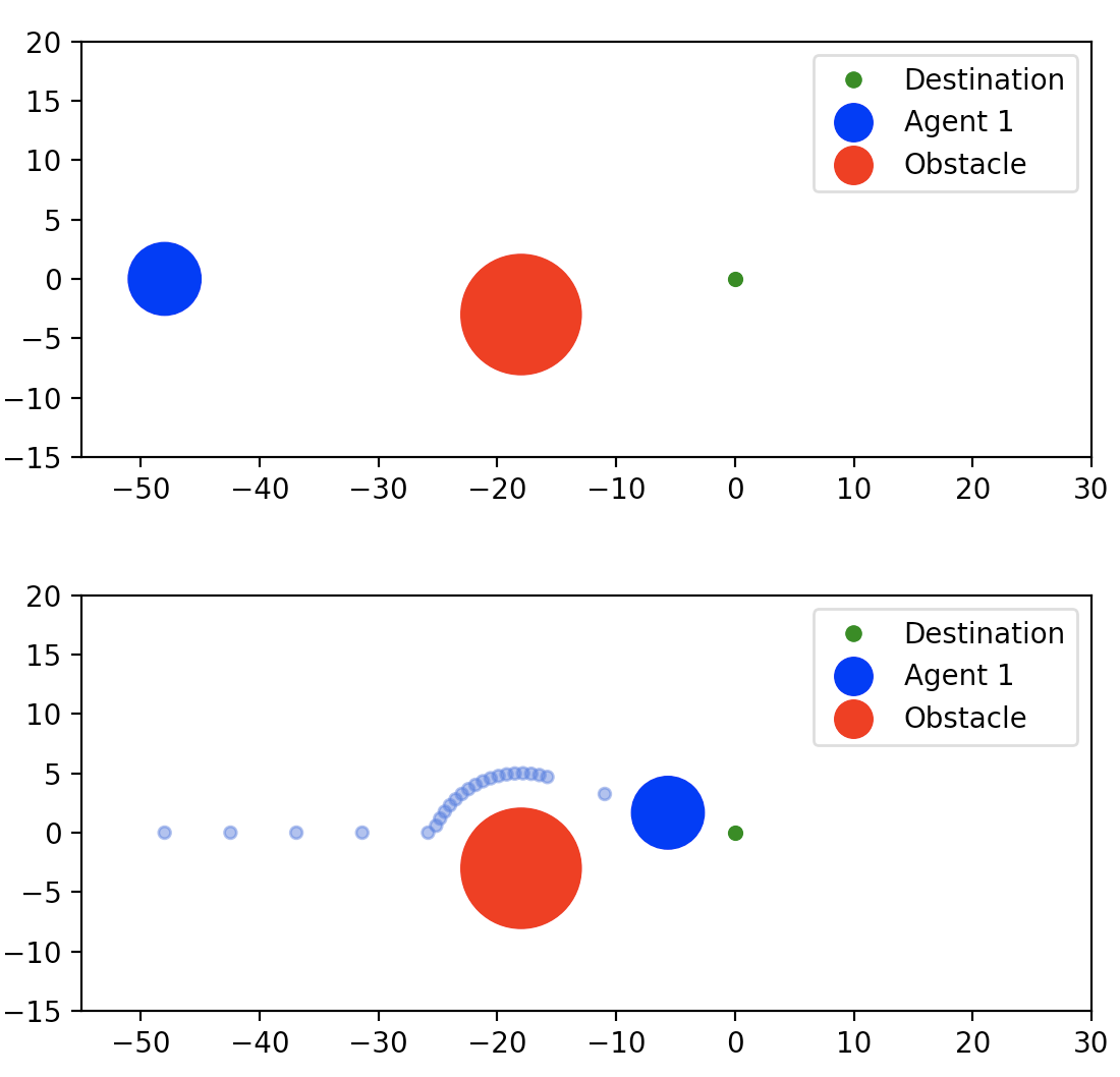
Figure 8: Illustration for Example 3.3 at $t=0$ and $t=T$

Example 3.3

In this example, we consider the case where the obstacle ${\bf x}^{obs}$ is not collinear with ${\bf x}^{0}$ and ${\bf x}^{des}$ (see Figure 8) with the following data:

$$\begin{cases}T=6,\;{\bf x}_{0}=(-48,0),\;{\bf x}^{obs}=(-18,-3),\;{\bf x}^{des}=(0,0)\\ r=5,\;L=3.\end{cases}$$

The performances of the agent in various cases of $\tau$ are shown in the following table.

$\tau$	$\overline{a}$	$t_{f}$	$t_{l}$	$J[\overline{x},\overline{a}]$
1.0	2.771724	1.018491	5.275958	23.107381
2.0	2.764543	1.021136	5.289662	46.095035
3.0	2.757400	1.023782	5.303366	68.963889
4.0	2.750293	1.026427	5.317069	91.714863
5.0	2.743223	1.029072	5.330773	114.348866
6.0	2.736189	1.031718	5.344477	136.866796
7.0	2.729191	1.034363	5.358181	159.269545
8.0	2.722229	1.037009	5.371885	181.557995
9.0	2.715302	1.039654	5.385588	203.733017
10.0	2.708411	1.042300	5.399292	225.795476

In the cases where the obstacle is not on the way from the agent to the destination, the problem becomes trivial since there is no sweeping effect involved; see Figure 9.

Example 3.4

Consider the optimal control problem with the following data:

$$\begin{cases}T=6,\;{\bf x}_{0}=(-48,0),\;{\bf x}^{obs}=(-30,-9),\;{\bf x}^{des}=(0,0)\\ r=5,\;L=3.\end{cases}$$

In this case, the agent is free to reach the destination without any contact with the obstacle. We deduce from (3.6) that

$$\dot{\overline{\bf x}}(t)=-s\overline{a}\dfrac{\overline{\bf x}(t)-{\bf x}^{des}}{\left\|\overline{\bf x}(t)-{\bf x}^{des}\right\|},\quad\forall t\in[0,T]$$

and hence

$$J =\frac{1}{2}\left\|\overline{\bf x}(T)-{\bf x}^{des}\right\|^{2}+\dfrac{\tau T}{2}\overline{a}^{2}$$

$$=\frac{1}{2}\left\|x_{0}+s\overline{a}T\dfrac{{\bf x}^{des}-{\bf x}^{0}}{\|{\bf x}^{des}-{\bf x}^{0}\|}-{\bf x}^{des}\right\|^{2}+\dfrac{\tau T}{2}\overline{a}^{2}$$

$$=\frac{1}{2}\|{\bf x}^{des}-{\bf x}^{0}\|^{2}\left[\dfrac{1}{\|{\bf x}^{des}-{\bf x}^{0}\|}s\overline{a}T-1\right]^{2}+\dfrac{\tau T}{2}\overline{a}^{2}.$$

The optimal value of $\overline{a}$ and of $J[{\bf x},\overline{a}]$ are provided in the following table depending on $\tau$.

$\tau$	$\overline{a}$	$t_{f}$	$t_{l}$	$J[\overline{x},\overline{a}]$
1.0	0.9974025924461699	empty	empty	2.992207792207821
2.0	0.9948186479096565	empty	empty	5.968911917098474
3.0	0.992248057110637	empty	empty	8.930232558139565
4.0	0.9896907167795382	empty	empty	11.876288659793842
5.0	0.9871465247276625	empty	empty	14.807197943444757
6.0	0.984615379889146	empty	empty	17.72307692307695
7.0	0.9820971819338324	empty	empty	20.624040920716144
8.0	0.9795918320755072	empty	empty	23.510204081632683
9.0	0.9770992320887493	empty	empty	26.381679389313003
10.0	0.9746192847468523	empty	empty	29.23857868020307

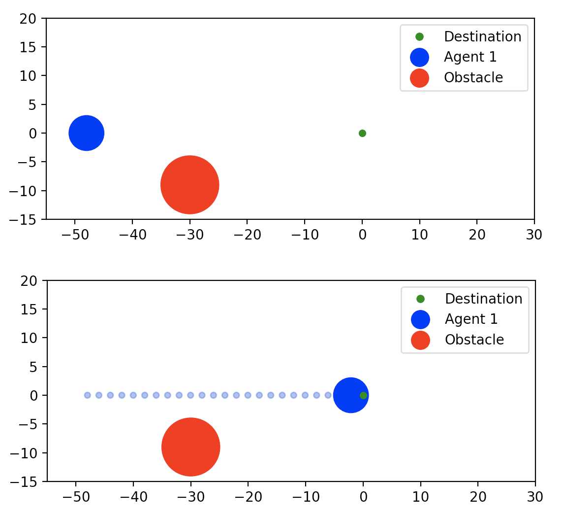
Figure 9: Illustration for Example 3.4 at $t=0$ and $t=T$

4 Controlled Crowd Motion Models with Multiple Agents and Multiple Obstacles

Our goal in this section is to study the crowd motion models with several agents and multiple obstacles. In what follows we consider $n$ agents $(n\geq 2)$ in the crowd motion model with $m$ obstacles in a given domain $\Omega\subset\mathbb{R}^{2}$. Our goal here is to search for an optimal strategy to drive all agents to a desired target with the minimum effort during a given time interval $[0,T]$. Following the mathematical framework in section 2 and in [7] we identify $n$ agents and $m$ obstacles to inelastic disks with different radii $L_{i}$ and $r_{i}$ whose centers are denoted by ${\bf x}_{i}=(x_{i1},x_{i2})$ and ${\bf x}^{obs}_{k}=(x^{obs}_{k1},x^{obs}_{k2})$ respectively for $i=1,\ldots,n$ and $k=1,\ldots,m$. To reflect the nonoverlapping of multiple agents and obstacles in this setting, the set of admissible configurations in (3.1) should be replaced by

$$C_{1}=\left\{{\bf x}\in\mathbb{R}^{2n}\big{|}\;D_{ij}({\bf x})\geq 0,\;\forall i<j,i,j\in\{1,\ldots,n\},\;D^{obs}_{ik}({\bf x})\geq 0,\forall i=1,\ldots,n,\;\forall k=1,\ldots,m\right\}$$ (4.1)

where $D_{ij}({\bf x}):=\left\|{\bf x}_{i}-{\bf x}_{j}\right\|-(L_{i}+L_{j})$ and $D^{obs}_{ik}({\bf x}):=\left\|{\bf x}_{i}-{\bf x}^{obs}_{k}\right\|-(L_{i}+r_{k})$ for $i=1,\ldots,n$ and for $k=1,\ldots,m$. Note that agent $i$ and $j$ will interact with each other when they are in contact, i.e. $D_{ij}({\bf x})=0$, while the interaction between agent $i$ and obstacle $k$ is a one-way interaction since – if the agent is close enough to the obstacle he/she will move away from it but the obstacle has no reaction to the agent. Thus the interactions among agents and interactions between agents and obstacles should be treated independently. Therefore the sweeping set $C_{1}$ in this framework is significantly different from the one in [13] (see [7] for more details). Motivated from the work in [7] we consider the following optimal control problem

$$\mbox{minimize}\;\;J[x,a]=\frac{1}{2}\left\|{\bf x}(T)-{\bf x}^{des}\right\|^{2}+\frac{\tau}{2}\int^{T}_{0}\left\|a(t)\right\|^{2}dt$$ (4.2)

over the control functions $a(\cdot)\in L^{2}([0,T];\mathbb{R}^{n})$ and the corresponding trajectory ${\bf x}(\cdot)\in W^{1,2}([0,T];\mathbb{R}^{2n})$ of the nonconvex sweeping process

$$\begin{cases}\dot{\bf x}(t)\in-N_{C}({\bf x}(t))+U({\bf x}(t),a(t))\;\;\mbox{a.e.}\;\;t\in[0,T],\\ {\bf x}(0)={\bf x}_{0}\in C_{1}\end{cases}$$ (4.3)

where the set $C_{1}$ is given in (4.1), where the desired velocity $U({\bf x},a)$ is given by

$$U({\bf x},a) =\left(-a_{1}s_{1}\nabla D^{des}({\bf x}_{1}),\ldots,-a_{n}s_{n}\nabla D^{des}({\bf x}_{n})\right)$$

$$=\left(-a_{1}s_{1}\dfrac{{\bf x}_{1}-{\bf x}^{des}_{1}}{\left\|{\bf x}_{1}-{\bf x}^{des}_{1}\right\|},\ldots,-a_{n}s_{n}\dfrac{{\bf x}_{n}-{\bf x}^{des}_{n}}{\left\|{\bf x}_{n}-{\bf x}^{des}_{n}\right\|}\right)$$

where ${\bf x}^{des}=\left({\bf x}^{des}_{1},\ldots,{\bf x}^{des}_{n}\right)\in\mathbb{R}^{2n}$ stands for the desired destination that the agents aim to, and where $\tau$ is a given constant. The objective of all the agents here is to minimize their distances to the desired destinations using the minimum control effort. The scalar $\tau\geq 0$ in (4.2) is a trade-off between the distance and the energy. Let us next derive a set of necessary optimality conditions for our optimal control problem in (4.2) – (4.3).

Theorem 4.1

(necessary optimality conditions for optimization of controlled crowd motions with multiple agents and obstacles) Let $(\overline{\bf x}(\cdot),\overline{\bf a}(\cdot))\in W^{2,\infty}([0,T];\mathbb{R}^{2n}\times\mathbb{R}^{n})$ be a strong local minimizer for the controlled crowd motion problem in (4.2) – (4.3). Then there exist $\lambda\geq 0$, $\eta_{ij}(\cdot)\in L^{2}([0,T];\mathbb{R}_{+}),\eta^{obs}_{ij}(\cdot)\in L^{2}([0,T];\mathbb{R}_{+})$ $(i,j=1,\ldots,n)$ well defined at $t=T$, ${\bf w}(\cdot)=({\bf w}^{x}(\cdot),{\bf w}^{a}(\cdot))\in L^{2}([0,T];\mathbb{R}^{3n})$, ${\bf v}(\cdot)=({\bf v}^{x}(\cdot),{\bf v}^{a}(\cdot))\in L^{2}([0,T];\mathbb{R}^{3n})$, an absolutely continuous vector function ${\bf p}(\cdot)=({\bf p}^{x}(\cdot),{\bf p}^{a}(\cdot))\in W^{1,2}([0,T];\mathbb{R}^{2n})$, a measure $\gamma\in C^{*}([0,T];\mathbb{R}^{2n})$ on $[0,T]$, and a vector function ${\bf q}(\cdot)=({\bf q}^{x}(\cdot),{\bf q}^{a}(\cdot))\colon[0,T]\to\mathbb{R}^{3n}$ of bounded variation on $[0,T]$ such that the following conditions are satisfied:

1. ${\bf w}(t)=(0,\overline{a}(t)),\;\;{\bf v}(t)=(0,0)$ for a.e. $t\in[0,T]$;

2. $\dot{\overline{\bf x}}(t)=\left(-\overline{a}_{1}(t)s_{1}\dfrac{\overline{\bf x}_{1}(t)-{\bf x}^{des}_{1}}{\left\|\overline{\bf x}_{1}(t)-{\bf x}^{des}_{1}\right\|},\ldots,-\overline{a}_{n}(t)s_{n}\dfrac{\overline{\bf x}_{n}-{\bf x}^{des}_{n}}{\left\|\overline{\bf x}_{n}-{\bf x}^{des}_{n}\right\|}\right)$
   $+\displaystyle\bigg{(}-\sum_{j>1}\eta_{1j}(t)\dfrac{\overline{\bf x}_{j}(t)-\overline{\bf x}_{1}(t)}{\|\overline{\bf x}_{j}(t)-\overline{\bf x}_{1}(t)\|}-\sum^{m}_{j=1}\eta^{obs}_{1j}\dfrac{{{\bf x}^{obs}_{j}}-\overline{\bf x}_{1}(t)}{\left\|{{\bf x}^{obs}_{j}}-\overline{\bf x}_{1}(t)\right\|},\ldots,\sum_{i<j}\eta_{ij}(t)\dfrac{\overline{\bf x}_{j}(t)-\overline{\bf x}_{i}(t)}{\|\overline{\bf x}_{j}(t)-\overline{\bf x}_{i}(t)\|}$
   $\displaystyle-\sum_{i>j}\eta_{ji}(t)\dfrac{\overline{\bf x}_{i}(t)-\overline{\bf x}_{j}(t)}{\|\overline{\bf x}_{i}(t)-\overline{\bf x}_{j}(t)\|}-\sum^{m}_{i=1}\eta^{obs}_{ji}\dfrac{{{\bf x}^{obs}_{i}}-\overline{\bf x}_{j}(t)}{\left\|{{\bf x}^{obs}_{i}}-\overline{\bf x}_{j}(t)\right\|},\displaystyle\ldots,\sum_{j<n}\eta_{jn}(t)\dfrac{\overline{\bf x}_{n}(t)-\overline{\bf x}_{j}(t)}{\|\overline{\bf x}_{n}(t)-\overline{\bf x}_{j}(t)\|}$
   $-\displaystyle\sum^{m}_{j=1}\eta^{obs}_{nj}(t)\dfrac{{{\bf x}^{obs}_{i}}-\overline{\bf x}_{n}(t)}{\left\|{{\bf x}^{obs}_{i}}-\overline{\bf x}_{n}(t)\right\|}\bigg{)}$;

3. $\begin{cases}\left\|\overline{\bf x}_{i}(t)-\overline{\bf x}_{j}(t)\right\|>L_{i}+L_{j}\Longrightarrow\eta_{ij}(t)=0,\forall i<j,\\ \left\|\overline{\bf x}_{i}(t)-{\bf x}^{obs}_{k}\right\|>L_{i}+r_{k}\Longrightarrow\eta^{obs}_{ik}(t)=0,\forall i=1,\ldots,n,\forall k=1,\ldots,m\end{cases}$ for a.e. $t\in[0,T]$;

4. $\begin{cases}\eta_{ij}(t)>0\Longrightarrow\left\langle{\bf q}^{x}_{j}(t)-{\bf q}^{x}_{i}(t),\overline{\bf x}_{j}(t)-\overline{\bf x}_{i}(t)\right\rangle=0,\forall i<j\\ \eta^{obs}_{ik}(t)>0\Longrightarrow\left\langle{\bf q}_{i}^{x}(t),{\bf x}^{obs}_{k}-\overline{\bf x}_{i}(t)\right\rangle=0,\forall i=1,\ldots,n,\forall k=1,\ldots,m\end{cases}$ for a.e. $t\in[0,T]$;

5. $\dot{\bf p}(t)=\bigg{(}0,\lambda\overline{a}_{1}(t)-s_{1}\left\langle{\bf q}^{x}_{1}(t),\dfrac{\overline{\bf x}_{1}(t)-{\bf x}^{des}_{1}}{\left\|\overline{\bf x}_{1}(t)-{\bf x}^{des}_{1}\right\|}\right\rangle,\ldots,\lambda\overline{a}_{n}(t)-s_{n}\left\langle{\bf q}^{x}_{n}(t),\dfrac{\overline{\bf x}_{n}(t)-{\bf x}^{des}_{n}}{\left\|\overline{\bf x}_{n}(t)-{\bf x}^{des}_{n}\right\|}\right\rangle\bigg{)}$
   for a.e. $t\in[0,T]$;

6. ${\bf q}^{x}(t)={\bf p}^{x}(t)+\gamma([t,T])$ for a.e. $t\in[0,T]$;

7. ${\bf q}^{a}(t)={\bf p}^{a}(t)=0$ for a.e. $t\in[0,T]$;

8. ${\bf p}^{x}(T)+\lambda(\overline{\bf x}(T)-{\bf x}^{des})$
   $=\displaystyle\bigg{(}-\sum_{j>1}\eta_{1j}(T)\dfrac{\overline{\bf x}_{j}(T)-\overline{\bf x}_{1}(T)}{\|\overline{\bf x}_{j}(T)-\overline{\bf x}_{1}(T)\|}-\sum^{m}_{j=1}\eta^{obs}_{1j}\dfrac{{{\bf x}^{obs}_{j}}-\overline{\bf x}_{1}(T)}{\left\|{{\bf x}^{obs}_{j}}-\overline{\bf x}_{1}(T)\right\|},\ldots,\sum_{i<j}\eta_{ij}(T)\dfrac{\overline{\bf x}_{j}(T)-\overline{\bf x}_{i}(T)}{\|\overline{\bf x}_{j}(T)-\overline{\bf x}_{i}(T)\|}$
   $\displaystyle-\sum_{i>j}\eta_{ji}(T)\dfrac{\overline{x}_{i}(T)-\overline{x}_{j}(T)}{\|\overline{x}_{i}(T)-\overline{x}_{j}(T)\|}-\sum^{m}_{i=1}\eta^{obs}_{ji}\dfrac{{{\bf x}^{obs}_{i}}-\overline{\bf x}_{j}(T)}{\left\|{{\bf x}^{obs}_{i}}-\overline{\bf x}_{j}(T)\right\|},\displaystyle\ldots,\sum_{j<n}\eta_{jn}(T)\dfrac{\overline{\bf x}_{n}(T)-\overline{\bf x}_{j}(T)}{\|\overline{\bf x}_{n}(T)-\overline{\bf x}_{j}(T)\|}$
   $-\displaystyle\sum^{m}_{j=1}\eta^{obs}_{nj}(T)\dfrac{{{\bf x}^{obs}_{i}}-\overline{\bf x}_{j}(T)}{\left\|{{\bf x}^{obs}_{i}}-\overline{\bf x}_{j}(T)\right\|}\bigg{)}$;

9. ${\bf p}^{a}(T)=0$;

10. $\lambda+\|{\bf p}^{x}(T)\|>0$.

Proof. To verify the claimed set of necessary optimality conditions for our dynamical optimization (4.2) – (4.3) we elaborate the arguments similar to those in the proof of [13, Theorem 3.1] for the new setting of the controlled crowd motion model with obstacles under consideration with $g_{ij}({\bf x}):=D_{ij}({\bf x})=\left\|{\bf x}_{i}-{\bf x}_{j}\right\|-(L_{i}+L_{j})$ for $i<j$, where $i,j\in\{1,\ldots,n\}$ and $g^{obs}_{ik}({\bf x}):=D^{obs}_{ik}({\bf x})=\left\|{\bf x}_{i}-{\bf x}^{obs}_{k}\right\|-(L_{i}+r_{k})$ for $i=1,\ldots,n$ and $k=1,\ldots,m$. Then the functions $g_{ij}$ and $g^{obs}_{ik}$ are convex, belong to the spaces $\mathcal{C}^{2}(V_{ij})$ and $\mathcal{C}^{2}(V^{obs}_{ik})$ respectively with $V_{ij}$ and $V^{obs}_{ij}$ given by

$$V_{ij}\colon=\left\{{\bf x}\in\mathbb{R}^{2n}\big{|}\;\left\|{\bf x}_{i}-{\bf x}_{j}\right\|>\frac{1}{2}(L_{i}+L_{j})\right\}$$

for $i<j$, where $i,j\in\{1,\ldots,n\}$,

$$V^{obs}_{ik}\colon=\left\{{\bf x}\in\mathbb{R}^{2n}\big{|}\;\left\|{\bf x}_{i}-{\bf x}^{obs}_{k}\right\|>\frac{1}{2}(L_{i}+r_{k})\right\}$$

for $i=1,\ldots,n$ and $k=1,\ldots,m$ and satisfy estimate (2.3) in [13] with

$$c\colon=\min\left\{\min_{\begin{subarray}{c}i<j\\ i,j\in\{1,\ldots,n\}\end{subarray}}\left\{\dfrac{L_{i}+L_{j}}{\sqrt{2}}\right\},\min_{\begin{subarray}{c}i=1,\ldots,n\\ k=1,\ldots,m\end{subarray}}\left\{\dfrac{L_{i}+r_{k}}{\sqrt{2}}\right\}\right\}.$$

It is obvious that

$$\begin{cases}\left\|\nabla g_{ij}({\bf x})\right\|=\sqrt{2}\mbox{ and }\left\|\nabla g^{obs}_{ik}({\bf y})\right\|=1,\\ \left\|\nabla^{2}g_{ij}({\bf x})\right\|\leq\dfrac{2}{L_{i}+L_{j}}\mbox{ and }\left\|\nabla^{2}g^{obs}_{ik}({\bf y})\right\|\leq\dfrac{2}{L_{i}+r_{k}}\end{cases}$$

for ${\bf x}\in V_{ij}$ and ${\bf y}\in V^{obs}_{ik}$ respectively. Finally, it follows from [39, Proposition 4.7] that there exist some $\beta_{1}>1$ and $\beta_{2}>1$ such that

$$\begin{cases}\sum_{(i,j)\in I_{1}({\bf x})}\alpha_{ij}\left\|\nabla g_{ij}({\bf x})\right\|\leq\beta_{1}\left\|\sum_{(i,j)\in I_{1}({\bf x})}\alpha_{ij}\nabla g_{ij}({\bf x})\right\|\\[8.61108pt] \sum_{(i,k)\in I_{2}({\bf x})}\alpha_{ik}\left\|\nabla g^{obs}_{ik}({\bf x})\right\|\leq\beta_{2}\left\|\sum_{(i,k)\in I_{2}({\bf x})}\alpha_{ik}\nabla g^{obs}_{ik}({\bf x})\right\|\end{cases}$$

for all ${\bf x}\in C_{1}$, with

$$I_{1}({\bf x})\colon=\left\{(i,j)|\;g_{ij}({\bf x})=0,\;i>j\right\},$$

$$I_{2}({\bf x})\colon=\left\{(i,k)|\;g^{obs}_{ik}({\bf x})=0,\;i=1,\ldots,n,\;k=1,\ldots,m\right\},$$

$\alpha_{ij}\geq 0$ and $\alpha_{ik}\geq 0$, which justifies the validity of inequality (2.5) in [13]. This completes the proof of the theorem. $\hfill\quad\square$

Let us next try to find the optimal control strategy for driving the agents to the desired targets with the minimum effort. To reduce the complexity of the problem we assume that the control function $\overline{\bf a}(\cdot)$ is constant over the interval $[0,T]$, i.e. $\overline{\bf a}(t)=\overline{\bf a}=(\overline{a}_{1},\ldots,\overline{a}_{n})$ for all $t\in[0,T]$. Note that equation (2) shows us a relationship between the actual velocity $\dot{\bf x}(t)$ and the controlled desired velocity

$$U(\overline{\bf x}(t),\overline{\bf a}(t))=\left(-\overline{a}_{1}s_{1}\dfrac{\overline{\bf x}_{1}-{\bf x}^{des}_{1}}{\left\|\overline{\bf x}_{1}-{\bf x}^{des}_{1}\right\|},\ldots,-\overline{a}_{n}s_{n}\dfrac{\overline{\bf x}_{n}-{\bf x}^{des}_{n}}{\left\|\overline{\bf x}_{n}-{\bf x}^{des}_{n}\right\|}\right)$$

while taking into account the interactions among the agents and obstacles. This relationship between two types of velocities of individual agent is reflected in the following equations

$$\begin{cases}\dot{\overline{\bf x}}_{1}(t)=-\overline{a}_{1}s_{1}\dfrac{\overline{\bf x}_{1}(t)-{\bf x}^{des}_{1}}{\left\|\overline{\bf x}_{1}(t)-{\bf x}^{des}_{1}\right\|}-\displaystyle\sum_{j>1}\eta_{1j}(t)\dfrac{\overline{\bf x}_{j}(t)-\overline{\bf x}_{1}(t)}{\|\overline{\bf x}_{j}(t)-\overline{\bf x}_{1}(t)\|}-\sum^{m}_{j=1}\eta^{obs}_{1j}(t)\dfrac{{{\bf x}^{obs}_{j}}-\overline{\bf x}_{1}(t)}{\left\|{{\bf x}^{obs}_{j}}-\overline{\bf x}_{1}(t)\right\|}\\[4.30554pt] \vdots\\ \dot{\overline{\bf x}}_{j}(t)=\displaystyle-\overline{a}_{j}s_{j}\dfrac{\overline{\bf x}_{j}-{\bf x}^{des}_{j}}{\left\|\overline{\bf x}_{j}-{\bf x}^{des}_{j}\right\|}+\sum_{i<j}\eta_{ij}(t)\dfrac{\overline{\bf x}_{j}(t)-\overline{\bf x}_{i}(t)}{\|\overline{\bf x}_{j}(t)-\overline{\bf x}_{i}(t)\|}-\sum_{i>j}\eta_{ji}(t)\dfrac{\overline{\bf x}_{i}(t)-\overline{\bf x}_{j}(t)}{\|\overline{\bf x}_{i}(t)-\overline{\bf x}_{j}(t)\|}\\[4.30554pt] -\displaystyle\sum^{m}_{i=1}\eta^{obs}_{ji}\dfrac{{{\bf x}^{obs}_{i}}-\overline{\bf x}_{j}(t)}{\left\|{{\bf x}^{obs}_{i}}-\overline{\bf x}_{j}(t)\right\|},\mbox{ for }1<j<n,\\[4.30554pt] \vdots\\[4.30554pt] \dot{\overline{\bf x}}_{n}(t)=\displaystyle-\overline{a}_{n}s_{n}\dfrac{\overline{\bf x}_{n}-{\bf x}^{des}_{n}}{\left\|\overline{\bf x}_{n}-{\bf x}^{des}_{n}\right\|}+\sum_{j<n}\eta_{jn}(t)\dfrac{\overline{\bf x}_{n}(t)-\overline{\bf x}_{j}(t)}{\|\overline{\bf x}_{n}(t)-\overline{\bf x}_{j}(t)\|}-\sum^{m}_{j=1}\eta^{obs}_{nj}(t)\dfrac{{{\bf x}^{obs}_{i}}-\overline{\bf x}_{n}(t)}{\left\|{{\bf x}^{obs}_{i}}-\overline{\bf x}_{n}(t)\right\|}.\end{cases}$$ (4.4)

Each equation means that on the way to the destination each individual agent has to consider not overlapping with other agents and not colliding with the obstacles; see Figure 10.

Figure 10: Crowd Motion Model with Multiple Agents and Obstacles

The implications in (3) tell us that if there is no contact between agents $i$ and $j$ or between agent $i$ and obstacle $k$, there is no interaction at all. In case of contact, the implications in (4) provide us some useful information about the interaction between agents $i$ and $j$ or between agent $i$ and obstacle $k$. To proceed further in this case, we deduce from equations (5) and (7) that

$$\lambda\overline{a}_{i}(t)=s_{i}\left\langle{\bf q}^{x}_{i}(t),\dfrac{\overline{\bf x}_{i}(t)-{\bf x}^{des}_{i}}{\left\|\overline{\bf x}_{i}(t)-{\bf x}^{des}_{i}\right\|}\right\rangle$$ (4.5)

for $i=1,\ldots,n$ which tells us how the quantities ${\bf q}^{x}_{i}(t),\overline{\bf x}_{i}(t)$ and ${\bf x}^{des}_{i}$ relate to the control $\overline{a}_{i}(t)$. To simplify our writing necessary optimality conditions, let us introduce the following notations

$$\begin{cases}\alpha_{i}(t)=\angle(\overline{\bf x}_{i}(t)-{\bf x}^{des}_{i},{\bf i}),\forall i=1,\ldots,n,\\ \alpha_{ij}(t)=\angle(\overline{\bf x}_{j}(t)-\overline{\bf x}_{i}(t),{\bf i}),\forall i<j,i,j\in\{1,\ldots,n\},\\ \alpha^{obs}_{ik}(t)=\angle({\bf x}^{obs}_{k}-\overline{\bf x}_{i}(t),{\bf i}),\forall i=1,\ldots,n,\forall k=1,\ldots,m.\end{cases}$$ (4.6)

Then the system of differential equations (4.4) can be read as

$$\begin{cases}\dot{\overline{\bf x}}_{1}(t)=-\overline{a}_{1}s_{1}(\cos\alpha_{1}(t),\sin\alpha_{1}(t))-\displaystyle\sum_{j>1}\eta_{1j}(t)(\cos\alpha_{1j}(t),\sin\alpha_{1j}(t))-\sum^{m}_{j=1}\eta^{obs}_{1j}(t)(\cos\alpha^{obs}_{1j}(t),\sin\alpha^{obs}_{1j}(t))\\[4.30554pt] \vdots\\[4.30554pt] \dot{\overline{\bf x}}_{j}(t)=\displaystyle-\overline{a}_{j}s_{j}(\cos\alpha_{j}(t),\sin\alpha_{j}(t))+\sum_{i<j}\eta_{ij}(t)(\cos\alpha_{ij}(t),\sin\alpha_{ij}(t))-\sum_{i>j}\eta_{ji}(t)(\cos\alpha_{ji}(t),\sin\alpha_{ji}(t))\\[4.30554pt] -\displaystyle\sum^{m}_{i=1}\eta^{obs}_{ji}(\cos\alpha^{obs}_{ji}(t),\sin\alpha^{obs}_{ji}(t)),\mbox{ for }1<j<n,\\[4.30554pt] \vdots\\[4.30554pt] \dot{\overline{\bf x}}_{n}(t)=\displaystyle-\overline{a}_{n}s_{n}(\cos\alpha_{n}(t),\sin\alpha_{n}(t))+\sum_{j<n}\eta_{jn}(t)(\cos\alpha_{jn}(t),\sin\alpha_{jn}(t))-\sum^{m}_{j=1}\eta^{obs}_{nj}(t)(\cos\alpha^{obs}_{nj}(t),\sin\alpha^{obs}_{nj}(t))\end{cases}$$ (4.7)

To simplify the complexity of the problem, it is reasonable to assume that the agents only adjust their directions once they have contact with each other or with the obstacles and all agents aim to reach to the same destination, i.e. ${\bf x}^{des}_{i}={\bf x}^{des}_{j}$ for all $i,j\in\{1,2,\ldots,n\}$. If agents $i$ and $j$ are in contact, they would adjust their own velocities to the new identical one and remain it until the end of the process or until having contact with other agents or with the obstacles, i.e. $\dot{\overline{\bf x}}_{i}(t)=\dot{\overline{\bf x}}_{j}(t)$ during the contact-time interval.

Let us next explore more about the case when agents $i$ and $j$ are in contact. In this very situation it makes a perfect sense to expect that $\eta_{ij}(t^{f}_{ij})>0$ and hence we can deduce from the first implication in (4) that

$$\left\langle{\bf q}^{x}_{j}(t^{f}_{ij})-{\bf q}^{x}_{i}(t^{f}_{ij}),(\cos\alpha_{ij}(t^{f}_{ij}),\sin\alpha_{ij}(t^{f}_{ij}))\right\rangle=0$$

which is equivalent to

$$\left[q^{x}_{j1}(t^{f}_{ij})-q^{x}_{i1}(t^{f}_{ij})\right]\cos\alpha_{ij}(t^{f}_{ij})+\left[q^{x}_{j2}(t^{f}_{ij})-q^{x}_{i2}(t^{f}_{ij})\right]\sin\alpha_{ij}(t^{f}_{ij})=0.$$ (4.8)

This equation somehow provides us some useful information about the interaction between agents $i$ and $j$ at the contact time $t^{f}_{ij}$. To make use of equation (4.8), we rewrite equation (4.5) in the following form

$$\lambda\overline{a}_{i}=s_{i}q^{x}_{i1}(t)\cos\alpha_{i}(t)+s_{i}q^{x}_{i2}(t)\sin\alpha_{i}(t)$$ (4.9)

for all $t\in[0,T]$ and try to relate it to equation (4.8). Let us investigate the behaviors of agents $i$ and $j$ at the contact time $t=t^{f}_{ij}$ in two following cases.

Case 1: Agents $i$ and $j$ are collinear with the destination at $t=t^{f}_{ij}$.

Without loss of generality we assume that agent $i$ stays in front of agent $j$ relative to the destination. Then $\alpha_{i}(t^{f}_{ij})=\alpha_{j}(t^{f}_{ij})=\alpha_{ij}(t^{f}_{ij})$. Combing this together with (4.8) and (4.9) we come up to

$$\lambda s_{i}\overline{a}_{j}=\lambda s_{j}\overline{a}_{i}$$ (4.10)

which in turn implies that $s_{i}\overline{a}_{j}=s_{j}\overline{a}_{i}$ assuming that $\lambda>0$; otherwise we do not have enough information to proceed. Equation (4.10) provides us a useful relationship between agents $i$ and $j$ at the contact time. Let $t^{l}_{ij}$ denote the time they have contact with other agents or the obstacles, it is possible that $t^{l}_{ij}=T$. In this case, we have

$$\dot{\overline{\bf x}}_{i}(t)=\dot{\overline{\bf x}}_{j}(t)\mbox{ for all }t\in\left[t^{f}_{ij},t^{l}_{ij}\right].$$

This case can be treated as a version of the corridor setting considered in what follows.

Case 2: Agents $i$ and $j$ are not collinear with the destination at $t=t^{f}_{ij}$.

As mentioned before, two agents adjust their own velocities to the new identical one and remain it until the end of the process or until having contact with other agents or with the obstacles. In this particular case, equation (4.8) showing the relation between the agents cannot be fully utilized and hence we are not able to obtain (4.10).

To understand how our set of necessary optimality conditions derived in Theorem 4.1 can be used to solve the formulated dynamic optimization problems systematically, we consider several general crowd motion control problems for multiple agents in the corridor settings; we refer the reader to [10, 11] for more details.

The Controlled Crowd Motion Models with Multiple Agents in a Corridor

This part is devoted to the study of the crowd motion control problem for multiple agents ${\bf x}_{1},{\bf x}_{2},\ldots,{\bf x}_{n}$ in a corridor without any obstacles in general settings; see Figure 11. For our convenience, we assume that the destination is always on the right side of the agents, which implies that

$$\begin{cases}\alpha_{i}(t)=180^{\circ},\mbox{ for all }i=1,2,\ldots,n,\\ \alpha_{ii+1}(t)=0^{\circ},\mbox{for all }i=1,2,\ldots,n-1.\end{cases}$$

Then the differential relation in (4.5) can be read as

$$\begin{cases}\dot{\overline{\bf x}}_{1}(t)=(\overline{a}_{1}s_{1},0)-(\eta_{12}(t),0),\\ \vdots\\ \dot{\overline{\bf x}}_{j}(t)=(\overline{a}_{j}s_{j},0)+(\eta_{j-1j}(t)-\eta_{j+1j}(t),0),\mbox{ for }j=2,\ldots,n-1,\\ \vdots\\ \dot{\overline{\bf x}}_{n}(t)=(\overline{a}_{n}s_{n},0)+(\eta_{n-1n}(t),0).\end{cases}$$ (4.11)

Figure 11: Crowd Motion Models in a Corridor

The Crowd Motion Model with Two Agents

Let us first consider the motion model with two agents in general settings. It follows from (4.11) that the velocities of two agents are related via the following equations

$$\begin{cases}\dot{\overline{\bf x}}_{1}(t)=(\overline{a}_{1}s_{1}-\eta_{12}(t),0),\\ \dot{\overline{\bf x}}_{2}(t)=(\overline{a}_{2}s_{2}+\eta_{12}(t),0).\end{cases}$$ (4.12)

Consider the following cases:

Case 1: Two agents are in contact, i.e. $0\leq t^{f}_{12}\leq T$. In this case, they would adjust their own velocities to the new identical one and remain it until the end of the process in case of contact, i.e., $\dot{\overline{\bf x}}_{1}(t)=\dot{\overline{\bf x}}_{2}(t)$ for all $t\in[t^{f}_{12},T]$ (see Figure 13). This enables us to compute the quantity $\eta_{12}(t)$ generated by the normal cone $N^{P}_{C}(\overline{\bf x})$ as follows

$$\eta_{12}(t)=\frac{1}{2}(\overline{a}_{1}s_{1}-\overline{a}_{2}s_{2})>0$$ (4.13)

for all $t\in[t^{f}_{12},T]$. Moreover, the interaction between the agents is reflected via the equation $s_{2}\overline{a}_{1}=s_{1}\overline{a}_{2}$ by (4.10) or equivalently $\overline{a}_{1}=\dfrac{s_{1}}{s_{2}}\overline{a}_{2}$ which allows us to compute $\eta_{12}(\cdot)$ explicitly as follows

$$\eta_{12}(t)=\begin{cases}0&\mbox{ if }t\in[0,t^{f}_{12})\\[4.30554pt] \dfrac{\overline{a}_{2}(s_{1}^{2}-s^{2}_{2})}{2s_{2}}&\mbox{ if }t\in[t^{f}_{12},T]\end{cases}$$ (4.14)

thanks to (4.13). Note that this formula tells us $s_{1}>s_{2}$, which always happens since agent 1 is farther to the destination compared to agent 2. In fact, we can select $s_{1}$ and $s_{2}$ by

$$s_{1}=\dfrac{\|{\bf x}^{des}-\overline{\bf x}_{1}(0)\|}{T}>\dfrac{\|{\bf x}^{des}-\overline{\bf x}_{2}(0)\|}{T}=s_{2}.$$

The value of the scalar function $\eta_{12}(\cdot)$ during the contact time interval $[t^{f}_{12},T]$ basically tells us some information about the interaction effort between two agents: each should contribute one half of the quantity $(\overline{a}_{1}s_{1}-\overline{a}_{2}s_{2})$ in such a way that agent 1 should slow down and agent 2 should speed up with the same quantity $\eta_{12}(t)=\frac{1}{2}(\overline{a}_{1}s_{1}-\overline{a}_{2}s_{2})$ in order to balance out their velocities.

Next using the Newton-Leibniz formula for (4.12) gives us

$$\begin{cases}\overline{\bf x}_{1}(t)=\overline{\bf x}_{1}(0)+(t\overline{a}_{1}s_{1}-t\eta_{12}(t^{f}_{12})+t^{f}_{12}\eta_{12}(t^{f}_{12}),0)\\[4.30554pt] \overline{\bf x}_{2}(t)=\overline{\bf x}_{2}(0)+(t\overline{a}_{2}s_{2}+t\eta_{12}(t^{f}_{12})-t^{f}_{12}\eta_{12}(t^{f}_{12}),0)\end{cases}$$ (4.15)

for all $t\in[t^{f}_{12},T]$ taking into account ${\bf x}_{22}(0)={\bf x}_{12}(0)$. We then deduce from the fact $\left\|\overline{x}_{2}(t)-x_{1}(t)\right\|=L_{2}+L_{1}$ for all $t\in[t^{f}_{12},T]$ that

$$\left|-2t^{f}_{12}\eta_{12}(t^{f}_{12})+\overline{x}_{21}(0)-\overline{x}_{11}(0)\right|=L_{1}+L_{2}$$

or equivalently

$$\begin{cases}t^{f}_{12}\eta_{12}(t^{f}_{12})=\frac{1}{2}\left[\overline{x}_{21}(0)-\overline{x}_{11}(0)\mp(L_{1}+L_{2})\right]:=\Lambda_{12}\\[4.30554pt] t^{f}_{12}=\dfrac{\Lambda_{12}}{\eta_{12}(t^{f}_{12})}.\end{cases}$$ (4.16)

Note that the first equation in (4.16) reduces to

$$t^{f}_{12}\eta_{12}(t^{f}_{12})=\frac{1}{2}\left[\overline{x}_{21}(0)-\overline{x}_{11}(0)-(L_{1}+L_{2})\right]=\Lambda_{12}$$

since the destination is assumed to be on the right side of the agents. This equation somehow tells us the contact time and the interaction effort between two agents rely on their initial positions. In summary, all terms $\overline{\bf x}_{1}(T),\overline{\bf x}_{2}(T),$ and $t^{f}_{12}$ can be expressed in terms of control $\overline{a}_{2}$, so the cost functional given by

$$J[\overline{\bf x},\overline{a}]=\frac{1}{2}\left[\left\|\overline{\bf x}_{1}(T)-{\bf x}^{des}\right\|^{2}+\left\|\overline{\bf x}_{2}(T)-{\bf x}^{des}\right\|^{2}\right]+\dfrac{\tau T}{2}(\overline{a}_{1}^{2}+\overline{a}_{2}^{2})$$ (4.17)

can also be expressed in terms of $\overline{a}_{2}$ as well. There are two possibilities regarding the contact time $t^{f}_{12}$.

Case 1a: The agents are initially in contact, i.e. $\overline{\bf x}_{21}(0)-\overline{\bf x}_{11}(0)=L_{1}+L_{2}$. In this very situation, we have $t^{f}_{12}=0$ and the agents are heading to the destination with the same velocity until the end of the process. Their trajectories can be computed as follows

$$\begin{cases}\overline{\bf x}_{1}(t)=\overline{\bf x}_{1}(0)+\left(t\overline{a}_{1}s_{1}-t\dfrac{\overline{a}_{2}(s_{1}^{2}-s^{2}_{2})}{2s_{2}},0\right)\\[8.61108pt] \overline{\bf x}_{2}(t)=\overline{\bf x}_{2}(0)+\left(t\overline{a}_{2}s_{2}+t\dfrac{\overline{a}_{2}(s_{1}^{2}-s^{2}_{2})}{2s_{2}},0\right),\end{cases}$$ (4.18)

and the cost functional is given explicitly by

$$J[\overline{\bf x},\overline{a}]=\frac{1}{2}\left[\left|\overline{\bf x}_{11}(0)+T\dfrac{\overline{a}_{2}(s_{1}^{2}+s^{2}_{2})}{2s_{2}}-{\bf x}^{des}_{1}\right|^{2}+\left|\overline{\bf x}_{21}(0)+T\dfrac{\overline{a}_{2}(s_{1}^{2}+s^{2}_{2})}{2s_{2}}-{\bf x}^{des}_{1}\right|^{2}\right]+\dfrac{\tau T\overline{a}_{2}^{2}(s_{1}^{2}+s^{2}_{2})}{2s_{2}^{2}}.$$ (4.19)

Minimizing this quadratic function with respect to $\overline{a}_{2}$ gives an optimal pair $(\overline{a}_{1},\overline{a}_{2})$ to our optimal control problem.

Case 1b: The agents are out of contact at the beginning i.e. $t^{f}_{12}>0.$ It then follows from (4.15), (4.16) and the fact $t^{f}_{12}\leq T$ that

$$\dfrac{\Lambda_{12}}{\eta_{12}(t^{f}_{12})}\leq T\iff\eta_{12}(t^{f}_{12})\geq\dfrac{\Lambda_{12}}{T}\iff\overline{a}_{2}\geq\dfrac{2s_{2}\Lambda_{12}}{T(s^{2}_{1}-s^{2}_{2})}$$ (4.20)

The cost functional in this case is

$$J[\overline{\bf x},\overline{a}] =\frac{1}{2}\bigg{[}\left\|\overline{\bf x}_{11}(0)+T\overline{a}_{1}s_{1}-T\eta_{12}(t^{f}_{12})+t^{f}_{12}\eta_{12}(t^{f}_{12})-{\bf x}^{des}_{1}\right\|^{2}$$ (4.21)

$$+\left\|\overline{\bf x}_{21}(0)+T\overline{a}_{2}s_{2}+T\eta_{12}(t^{f}_{12})-t^{f}_{12}\eta_{12}(t^{f}_{12})-{\bf x}^{des}_{1}\right\|^{2}\bigg{]}+\dfrac{\tau T\overline{a}_{2}^{2}(s_{1}^{2}+s^{2}_{2})}{2s_{2}^{2}}.$$

Minimizing this quadratic function with respect to $\overline{a}_{2}$ subject to constraint (4.20) gives an optimal pair $(\overline{a}_{1},\overline{a}_{2})$ to our optimal control problem.

Case 2: There is no contact between agents during the whole time interval $[0,T]$. Then the scalar function $\eta_{12}(\cdot)$ vanishes on $[0,T]$ due to the inactivity of the normal cone $N^{P}_{C}(\overline{\bf x})$. Thus the cost functional is simply given by

$$J[\overline{\bf x},\overline{a}]=\frac{1}{2}\left[\left|\overline{\bf x}_{11}(0)+T\overline{a}_{1}s_{1}-{\bf x}^{des}_{1}\right|^{2}+\left|\overline{\bf x}_{21}(0)+T\overline{a}_{2}s_{2}-{\bf x}^{des}_{1}\right|^{2}\right]+\dfrac{\tau T}{2}(\overline{a}_{1}^{2}+\overline{a}_{2}^{2}).$$ (4.22)

In this case we have

$$\left\|{\bf x}_{2}(t)-{\bf x}_{1}(t)\right\|=\left|\overline{x}_{21}(0)-\overline{x}_{11}(0)+t(\overline{a}_{2}s_{2}-\overline{a}_{1}s_{1})\right|>L_{1}+L_{2}$$

which in turn implies that

$$t(\overline{a}_{1}s_{1}-\overline{a}_{2}s_{2})<\overline{x}_{21}(0)-\overline{x}_{11}(0)-(L_{1}+L_{2})$$ (4.23)

for all $t\in[0,T]$.

$\bullet$ If $\overline{a}_{1}s_{1}<\overline{a}_{2}s_{2}$, inequality (4.23) holds true. This case means we can force agent 2 to move faster than agent 1 to ensure that they are out of contact until the end of the process.

$\bullet$ If $\overline{a}_{1}s_{1}>\overline{a}_{2}s_{2}$, inequality (4.23) implies that

$$T<\dfrac{\overline{x}_{21}(0)-\overline{x}_{11}(0)-(L_{1}+L_{2})}{\overline{a}_{1}s_{1}-\overline{a}_{2}s_{2}}$$ (4.24)

In this case although agent 1 is pushed to move faster than the other, the agents are still not in contact within a small period of time. The right hand side of (4.24) serves as an upper bound of the time they are out of contact depending on their initial positions.

Figure 12: Two Agents Before Contact

Figure 13: Two Agents After Contact

We summarize the above work in Algorithm 2. This can be considered as an extension of the work in [11] to general data settings. In what follows, we present two examples with distinct data sets illustrating the effectiveness of the proposed algorithm.

Example 4.2

Consider the controlled crowd motion problem with the following data:

$$\begin{cases}{\bf x}^{des}=(0,0),\;{\bf x}_{1}^{0}=(0,48),\;{\bf x}_{2}^{0}=(0,24),\\ T=6,\;L_{1}=L_{2}=3.\end{cases}$$

The performances of the agents are shown in the below table and Figure 14.

$\tau$	$\overline{a}_{1}$	$\overline{a}_{2}$	$t^{f}_{12}$	$J[\overline{x},\overline{a}]$
1.0	1.195021	0.597510	2.510417	14.377593
2.0	1.190083	0.595041	2.520833	19.710744
3.0	1.185185	0.592593	2.531250	25.000000
4.0	1.180328	0.590164	2.541667	30.245902
5.0	1.175510	0.587755	2.552083	35.448980
6.0	1.170732	0.585366	2.562500	40.609756
7.0	1.165992	0.582996	2.572917	45.728745
8.0	1.161290	0.580645	2.583333	50.806452
9.0	1.156626	0.578313	2.593750	55.843373
10.0	1.152000	0.576000	2.604167	60.840000

Although Example 14 and Example 3.2 share the same initial data, the performance results are completely different which evidently shows that the obstacle cannot be considered as an agent.

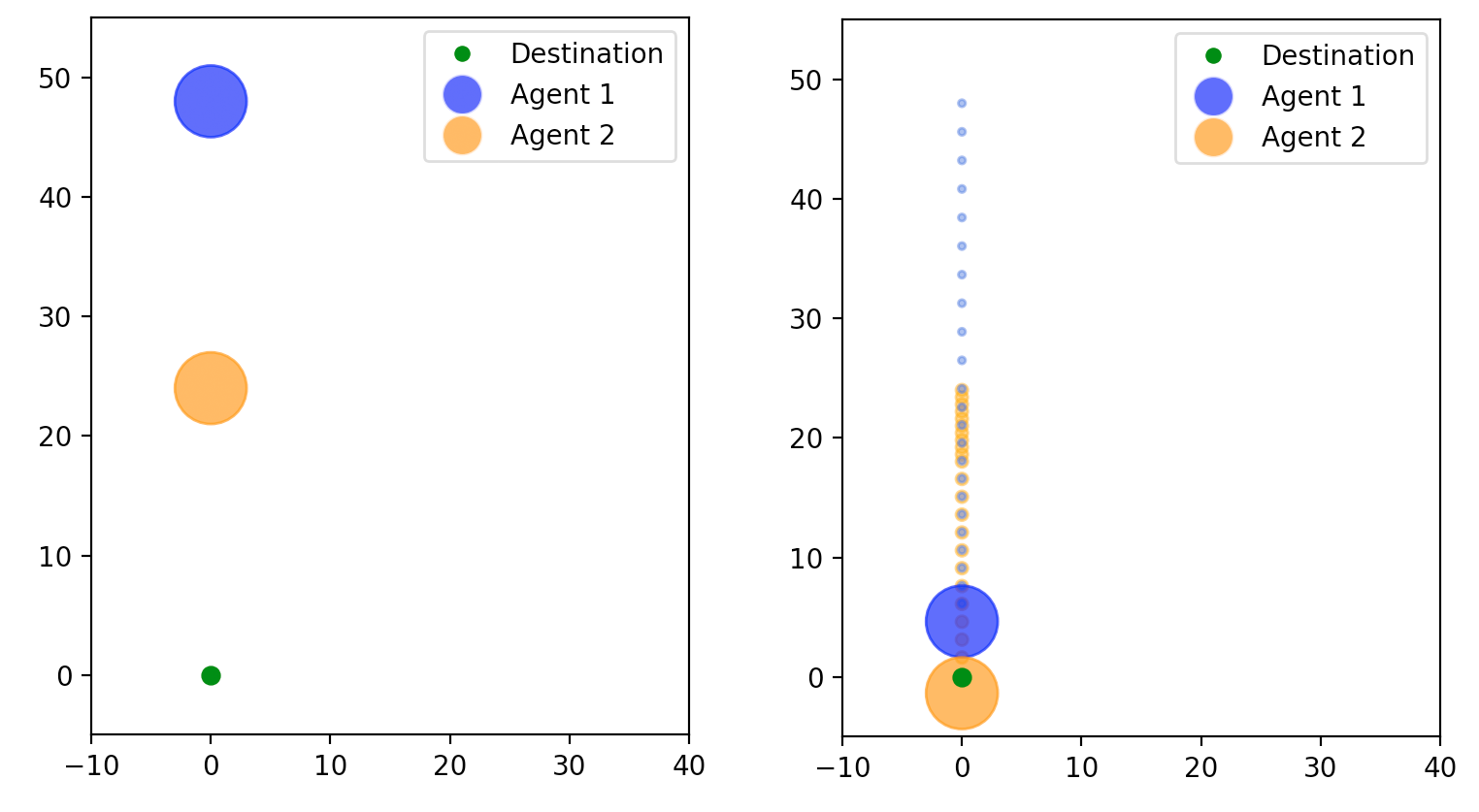
Figure 14: Illustration for Example 4.2 at $t=0$ and $t=T$

Example 4.3

Consider the controlled crowd motion problem with the following data (see Figure 15):

$$\begin{cases}{\bf x}^{des}=(0,0),\;{\bf x}_{1}^{0}=(-48,48),\;{\bf x}_{2}^{0}=(-24,24),\\ T=6,\;L_{1}=5,\;L_{2}=3.\end{cases}$$

The optimal value of $\overline{a}$ and of $J[\overline{\bf x},\overline{a}]$ are provided in the following table depending on $\tau$.

$\tau$	$\overline{a}_{1}$	$\overline{a}_{2}$	$t^{f}_{12}$	$J[\overline{x},\overline{a}]$
1.0	1.166355	0.728972	2.170803	21.685981
2.0	1.164179	0.727612	2.174861	27.350746
3.0	1.162011	0.726257	2.178918	32.994413
4.0	1.159851	0.724907	2.182976	38.617100
5.0	1.157699	0.723562	2.187033	44.218924
6.0	1.155556	0.722222	2.191091	49.800000
7.0	1.153420	0.720887	2.195149	55.360444
8.0	1.151291	0.719557	2.199206	60.900369
9.0	1.149171	0.718232	2.203264	66.419890
10.0	1.147059	0.716912	2.207321	71.919118

The performances of the agents are significantly better than the uncontrolled cases (with $\overline{a}_{1}=\overline{a}_{2}=1$), which is clearly shown in the below table.

$\tau$	$t^{f}_{12}$	$J[\overline{x}]$
1.0	4.114382	114.16
2.0	4.114382	120.16
3.0	4.114382	126.16
4.0	4.114382	132.16
5.0	4.114382	138.16
6.0	4.114382	144.16
7.0	4.114382	150.16
8.0	4.114382	156.16
9.0	4.114382	162.16
10.0	4.114382	168.16

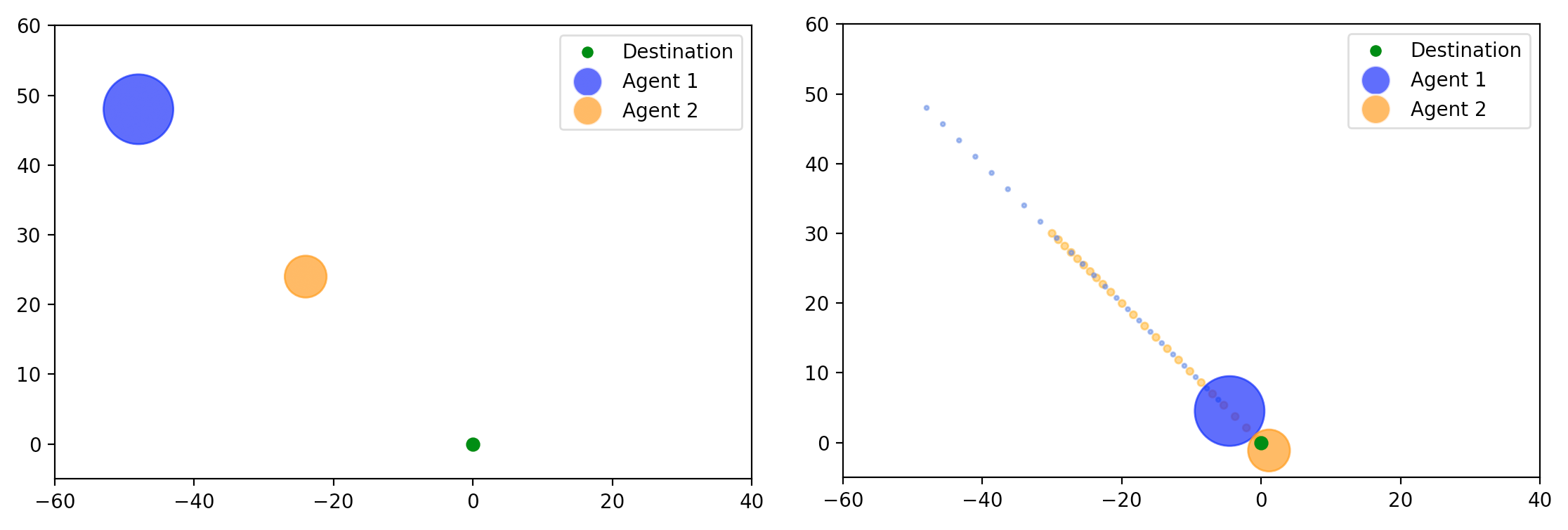
Figure 15: Illustration for Example 4.3 at $t=0$ and $t=T$

Remark 4.4

It is worth mentioning that the relation between $\overline{a}_{1}$ and $\overline{a}_{2}$ via equation (4.10) is very crucial for computational issues. Although one is still able to perform other computations and obtain the same solution without it by minimizing the cost functional with respect to $\overline{a}_{1}$ and $\overline{a}_{2}$, the computational complexity of Algorithm 2 in this case is remarkably worse. This clearly shows the importance and effectiveness of such a relation derived from the necessary conditions in Theorem 4.1. Furthermore, this relation also significantly reduces the complexity of the controlled crowd motion models with three or more agents which are much more involved than the cases of two agents.

The Crowd Motion Model with Three Agents

Now, let us consider crowd motion control problem for three agents $\overline{\bf x}_{1},\overline{\bf x}_{2},$ and $\overline{\bf x}_{3}$ in general settings. The differential relation in (4.11) reduces to

$$\begin{cases}\dot{\overline{\bf x}}_{1}(t)=(\overline{a}_{1}s_{1}-\eta_{12}(t),0),\\ \dot{\overline{\bf x}}_{2}(t)=(\overline{a}_{2}s_{2}+\eta_{12}(t)-\eta_{32}(t),0),\\ \dot{\overline{\bf x}}_{3}(t)=(\overline{a}_{3}s_{3}+\eta_{23}(t),0)\end{cases}$$ (4.25)

for a.e. $t\in[0,T]$.

Figure 16: Three Agents in a Corridor

In this very situation, agent 2 (the middle one) must take agents 1 and 3 into account. Note that $\eta_{32}(\cdot)=\eta_{23}(\cdot)$ in (4.25) since the interaction between any two agents is a two-way contact. Let us denote the first time three agents are in contact by $t^{f}_{123}$, then $\max\left\{t^{f}_{12},t^{f}_{23}\right\}\leq t^{f}_{123}$. We next investigate the behaviors of all agents at the contact times. Observe from (4.10) that $\overline{a}_{1}=\dfrac{s_{1}}{s_{2}}\overline{a}_{2}$ and $\overline{a}_{2}=\dfrac{s_{2}}{s_{3}}\overline{a}_{3}$ which are only valid during the contact times and hence imply that

$$\overline{a}_{2}=\dfrac{s_{2}}{s_{3}}\overline{a}_{3},\;\overline{a}_{1}=\dfrac{s_{1}}{s_{3}}\overline{a}_{3}$$ (4.26)

at $t=t^{f}_{123}$. It then follows from $\dot{\overline{\bf x}}_{1}(t^{f}_{12})=\dot{\overline{\bf x}}_{2}(t^{f}_{12})$ and $\dot{\overline{\bf x}}_{2}(t^{f}_{23})=\dot{\overline{\bf x}}_{3}(t^{f}_{23})$ that

$$\begin{cases}\eta_{12}(t^{f}_{12})=\frac{1}{2}\left[\overline{a}_{1}s_{1}-\overline{a}_{2}s_{2}+\eta_{23}(t^{f}_{12})\right]\\[8.61108pt] \eta_{23}(t^{f}_{23})=\frac{1}{2}\left[\overline{a}_{2}s_{2}-\overline{a}_{3}s_{3}+\eta_{12}(t^{f}_{23})\right]\end{cases}$$ (4.27)

which reflect the relations between the interaction efforts at the contact times. Since $\dot{\overline{\bf x}}_{1}(t^{f}_{123})=\dot{\overline{\bf x}}_{2}(t^{f}_{123})=\dot{\overline{\bf x}}_{3}(t^{f}_{123})$,

$$\begin{cases}\overline{a}_{1}s_{1}-\eta_{12}(t^{f}_{123})=\overline{a}_{2}s_{2}+\eta_{12}(t^{f}_{123})-\eta_{23}(t^{f}_{123})\\ \overline{a}_{2}s_{2}+\eta_{12}(t^{f}_{123})-\eta_{23}(t^{f}_{123})=\overline{a}_{3}s_{3}+\eta_{23}(t^{f}_{123})\end{cases}$$

which gives us

$$\begin{cases}\eta_{12}(t^{f}_{123})=\frac{1}{3}(2\overline{a}_{1}s_{1}-\overline{a}_{2}s_{2}-\overline{a}_{3}s_{3})\\[4.30554pt] \eta_{23}(t^{f}_{123})=\frac{1}{3}(\overline{a}_{1}s_{1}+\overline{a}_{2}s_{2}-2\overline{a}_{3}s_{3}).\end{cases}$$

Combining these relations with equations in (4.26) we can compute $\eta_{12}(t^{f}_{123})$ and $\eta_{23}(t^{f}_{123})$ in terms of $\overline{a}_{3}$ as follows

$$\begin{cases}\eta_{12}(t^{f}_{123})=\dfrac{(2s^{2}_{1}-s^{2}_{2}-s^{2}_{3})\overline{a}_{3}}{3s_{3}}\\[8.61108pt] \eta_{23}(t^{f}_{123})=\dfrac{(s^{2}_{1}+s^{2}_{2}-2s^{2}_{3})\overline{a}_{3}}{3s_{3}}.\end{cases}$$ (4.28)

Thus, the velocities of three agents during the time interval $[t^{f}_{123},T]$ are given by

$$\dot{\overline{\bf x}}_{1}(t)=\dot{\overline{\bf x}}_{2}(t)=\dot{\overline{\bf x}}_{3}(t)=\left(\dfrac{(s^{2}_{1}+s^{2}_{2}+s^{2}_{3})\overline{a}_{3}}{3s_{3}},0\right)\mbox{ for all }t\in[t^{f}_{123},T].$$ (4.29)

Consider the following cases.

$\bullet$ Case 1: $t^{f}_{12}<t^{f}_{23},$ i.e. agent 1 and agent 2 are in contact first.

Figure 17: Agents 1 and 2 are in contact first

In this case there is no contact between agent 2 and 3 at $t^{f}_{12}$, i.e. $\eta_{23}(t^{f}_{12})=0$, and $t^{f}_{23}=t^{f}_{123}$. Thus, the first equation in (4.27) implies

$$\eta_{12}(t^{f}_{12})=\frac{1}{2}(\overline{a}_{1}s_{1}-\overline{a}_{2}s_{2})>0$$

which reduces to (4.13). The scalar functions $\eta_{12}(\cdot)$ and $\eta_{23}(\cdot)$ showing the interactions among three agents are given by

$$\eta_{12}(t)=\begin{cases}0&\mbox{ if }t\in[0,t^{f}_{12})\\[4.30554pt] \frac{1}{2}(\overline{a}_{1}s_{1}-\overline{a}_{2}s_{2})=\dfrac{(s_{1}^{2}-s^{2}_{2})\overline{a}_{2}}{2s_{2}}&\mbox{ if }t\in[t^{f}_{12},t^{f}_{123})\\[4.30554pt] \frac{1}{3}(2\overline{a}_{1}s_{1}-\overline{a}_{2}s_{2}-\overline{a}_{3}s_{3})=\dfrac{(2s^{2}_{1}-s^{2}_{2}-s^{2}_{3})\overline{a}_{3}}{3s_{3}}&\mbox{ if }t\in[t^{f}_{123},T]\end{cases}$$ (4.30)

and

$$\eta_{23}(t)=\begin{cases}0&\mbox{ if }t\in[0,t^{f}_{12})\\[4.30554pt] 0&\mbox{ if }t\in[t^{f}_{12},t^{f}_{123})\\[4.30554pt] \frac{1}{3}(\overline{a}_{1}s_{1}+\overline{a}_{2}s_{2}-2\overline{a}_{3}s_{3})=\dfrac{(s^{2}_{1}+s^{2}_{2}-2s^{2}_{3})\overline{a}_{3}}{3s_{3}}&\mbox{ if }t\in[t^{f}_{123},T].\end{cases}$$ (4.31)

Here the values of the functions $\eta_{12}(\cdot)$ and $\eta_{23}(\cdot)$ during the contact time intervals are used to balance out the velocities of three agents to ensure they will not overlap.

Let us next compute the contact time $t^{f}_{12}$ for agents 1 and 2 and $t^{f}_{23}$ for agents 2 and 3 respectively. Indeed, we have

$$\begin{cases}\overline{\bf x}_{2}(t^{f}_{12})-\overline{\bf x}_{1}(t^{f}_{12})&=\overline{\bf x}_{2}(0)-\overline{\bf x}_{1}(0)+\left(t^{f}_{12}(\overline{a}_{2}s_{2}-\overline{a}_{1}s_{1}),0\right)\\[4.30554pt] &=\overline{\bf x}_{2}(0)-\overline{\bf x}_{1}(0)+\left(-2t^{f}_{12}\eta_{12}(t^{f}_{12}),0\right)\\[8.61108pt] \overline{\bf x}_{3}(t^{f}_{23})-\overline{\bf x}_{2}(t^{f}_{23})&=\overline{\bf x}_{3}(0)-\overline{\bf x}_{2}(0)+\left(t^{f}_{23}(\overline{a}_{3}s_{3}-\overline{a}_{2}s_{2}-\eta_{12}(t^{f}_{12}))+t^{f}_{12}\eta_{12}(t^{f}_{12}),0\right)\\[4.30554pt] &=\overline{\bf x}_{3}(0)-\overline{\bf x}_{2}(0)+\left(t^{f}_{23}\dfrac{2\overline{a}_{3}s_{3}-\overline{a}_{2}s_{2}-\overline{a}_{1}s_{1}}{2}+t^{f}_{12}\eta_{12}(t^{f}_{12}),0\right)\end{cases}$$

thanks to (4.30). It then follows from $\left\|\overline{\bf x}_{2}(t^{f}_{12})-\overline{\bf x}_{1}(t^{f}_{12})\right\|=L_{1}+L_{2}$ and $\left\|\overline{\bf x}_{3}(t^{f}_{23})-\overline{\bf x}_{1}(t^{f}_{23})\right\|=L_{2}+L_{3}$ that

$$\begin{cases}t^{f}_{12}\eta_{12}(t^{f}_{12})&=\dfrac{\overline{x}_{21}(0)-\overline{x}_{11}(0)-(L_{1}+L_{2})}{2}:=\Lambda_{12}\\[8.61108pt] t^{f}_{12}&=\dfrac{\Lambda_{12}}{\eta_{12}(t^{f}_{12})}\\[12.91663pt] \frac{3}{2}t^{f}_{23}\eta_{23}(t^{f}_{23})&=2\Lambda_{23}+\Lambda_{12}\\[8.61108pt] t^{f}_{123}=t^{f}_{23}&=\dfrac{2(2\Lambda_{23}+\Lambda_{12})}{3\eta_{23}(t^{f}_{123})}\leq T\\[8.61108pt] \mbox{where }\Lambda_{23}&\colon=\dfrac{\overline{x}_{31}(0)-\overline{x}_{21}(0)-(L_{2}+L_{3})}{2}\end{cases}$$ (4.32)

Combing (4.30) and (4.31) together with (4.32) enables us to compute the contact time $t^{f}_{12}$ and $t^{f}_{23}=t^{f}_{123}$ in terms of the controls $\overline{a}_{1},\overline{a}_{2}$ and $\overline{a}_{3}$. Now we have enough information to compute the velocities and hence the corresponding trajectories of three agents respectively as follows

$$\dot{\overline{\bf x}}_{1}(t)=\begin{cases}(\overline{a}_{1}s_{1},0)&\mbox{ if }t\in[0,t^{f}_{12})\\[8.61108pt] \left(\dfrac{(s^{2}_{1}+s^{2}_{2})\overline{a}_{2}}{2s_{2}},0\right)&\mbox{ if }t\in[t^{f}_{12},t^{f}_{123})\\[8.61108pt] \left(\dfrac{(s^{2}_{1}+s^{2}_{2}+s^{2}_{3})\overline{a}_{3}}{3s_{3}},0\right)&\mbox{ if }t\in[t^{f}_{123},T],\end{cases}$$

$$\dot{\overline{\bf x}}_{2}(t)=\begin{cases}(\overline{a}_{2}s_{2},0)&\mbox{ if }t\in[0,t^{f}_{12})\\[8.61108pt] \left(\dfrac{(s^{2}_{1}+s^{2}_{2})\overline{a}_{2}}{2s_{2}},0\right)&\mbox{ if }t\in[t^{f}_{12},t^{f}_{123})\\[8.61108pt] \left(\dfrac{(s^{2}_{1}+s^{2}_{2}+s^{2}_{3})\overline{a}_{3}}{3s_{3}},0\right)&\mbox{ if }t\in[t^{f}_{123},T],\end{cases}$$

$$\dot{\overline{\bf x}}_{3}(t)=\begin{cases}(\overline{a}_{3}s_{3},0)&\mbox{ if }t\in[0,t^{f}_{12})\\[8.61108pt] (\overline{a}_{3}s_{3},0)&\mbox{ if }t\in[t^{f}_{12},t^{f}_{123})\\[8.61108pt] \left(\dfrac{(s^{2}_{1}+s^{2}_{2}+s^{2}_{3})\overline{a}_{3}}{3s_{3}},0\right)&\mbox{ if }t\in[t^{f}_{123},T],\end{cases}$$

and

$$\overline{\bf x}_{1}(t)=\begin{cases}\overline{\bf x}_{1}(0)+(t\overline{a}_{1}s_{1},0)&\mbox{ if }t\in[0,t^{f}_{12})\\[8.61108pt] \overline{\bf x}_{1}(0)+\left(t^{f}_{12}\overline{a}_{1}s_{1}+(t-t^{f}_{12})\dfrac{(s^{2}_{1}+s^{2}_{2})\overline{a}_{2}}{2s_{2}},0\right)&\mbox{ if }t\in[t^{f}_{12},t^{f}_{123})\\[8.61108pt] \overline{\bf x}_{1}(0)+\left(t^{f}_{12}\overline{a}_{1}s_{1}+(t^{f}_{123}-t^{f}_{12})\dfrac{(s^{2}_{1}+s^{2}_{2})\overline{a}_{2}}{2s_{2}}+(t-t^{f}_{123})\dfrac{(s^{2}_{1}+s^{2}_{2}+s^{2}_{3})\overline{a}_{3}}{3s_{3}},0\right)&\mbox{ if }t\in[t^{f}_{123},T],\end{cases}$$ (4.33)

$$\overline{\bf x}_{2}(t)=\begin{cases}\overline{\bf x}_{2}(0)+(t\overline{a}_{2}s_{2},0)&\mbox{ if }t\in[0,t^{f}_{12})\\[8.61108pt] \overline{\bf x}_{2}(0)+\left(t^{f}_{12}\overline{a}_{2}s_{2}+(t-t^{f}_{12})\dfrac{(s^{2}_{1}+s^{2}_{2})\overline{a}_{2}}{2s_{2}},0\right)&\mbox{ if }t\in[t^{f}_{12},t^{f}_{123})\\[8.61108pt] \overline{\bf x}_{2}(0)+\left(t^{f}_{12}\overline{a}_{2}s_{2}+(t^{f}_{123}-t^{f}_{12})\dfrac{(s^{2}_{1}+s^{2}_{2})\overline{a}_{2}}{2s_{2}}+(t-t^{f}_{123})\dfrac{(s^{2}_{1}+s^{2}_{2}+s^{2}_{3})\overline{a}_{3}}{3s_{3}},0\right)&\mbox{ if }t\in[t^{f}_{123},T],\end{cases}$$ (4.34)

$$\overline{\bf x}_{3}(t)=\begin{cases}\overline{\bf x}_{3}(0)+(t\overline{a}_{3}s_{3},0)&\mbox{ if }t\in[0,t^{f}_{12})\\[8.61108pt] \overline{\bf x}_{3}(0)+(t\overline{a}_{3}s_{3},0)&\mbox{ if }t\in[t^{f}_{12},t^{f}_{123})\\[8.61108pt] \overline{\bf x}_{3}(0)+\left(t^{f}_{123}\overline{a}_{3}s_{3}+(t-t^{f}_{123})\dfrac{(s^{2}_{1}+s^{2}_{2}+s^{2}_{3})\overline{a}_{3}}{3s_{3}},0\right)&\mbox{ if }t\in[t^{f}_{123},T].\end{cases}$$ (4.35)

Therefore we are able to compute the final positions $\overline{\bf x}_{1}(T),\overline{\bf x}_{2}(T)$, and $\overline{\bf x}_{3}(T)$ by (4.33)–(4.35) and thus the cost functional given by

$$J[\overline{\bf x},\overline{a}]=\frac{1}{2}\sum^{3}_{i=1}\left\|\overline{\bf x}_{i}(T)-{\bf x}^{des}\right\|^{2}+\dfrac{\tau T}{2}(\overline{a}_{1}^{2}+\overline{a}_{2}^{2}+\overline{a}_{3}^{2})$$ (4.36)

in terms of $\overline{a}_{3}$.

$\bullet$ Case 2: $t^{f}_{23}<t^{f}_{12},$ i.e. agent 2 and agent 3 are in contact first.

Figure 18: Agents 2 and 3 are in contact first

In this case there is no contact between agent 1 and 2 at $t^{f}_{23}$, i.e. $\eta_{12}(t^{f}_{23})=0$, and $t^{f}_{12}=t^{f}_{123}$. Then (4.27) implies that

$$\begin{cases}\eta_{12}(t^{f}_{123})=\frac{1}{2}\left[\overline{a}_{1}s_{1}-\overline{a}_{2}s_{2}+\eta_{23}(t^{f}_{123})\right]\\[8.61108pt] \eta_{23}(t^{f}_{23})=\frac{1}{2}\left[\overline{a}_{2}s_{2}-\overline{a}_{3}s_{3}\right]\end{cases}$$

and hence the functions $\eta_{12}(\cdot)$ and $\eta_{23}(\cdot)$ are given by

$$\eta_{12}(t)=\begin{cases}0&\mbox{ if }t\in[0,t^{f}_{23,})\\[4.30554pt] 0&\mbox{ if }t\in[t^{f}_{23},t^{f}_{123})\\[4.30554pt] \frac{1}{3}(2\overline{a}_{1}s_{1}-\overline{a}_{2}s_{2}-\overline{a}_{3}s_{3})=\dfrac{(2s^{2}_{1}-s^{2}_{2}-s^{2}_{3})\overline{a}_{3}}{3s_{3}}&\mbox{ if }t\in[t^{f}_{123},T]\end{cases}$$ (4.37)

and

$$\eta_{23}(t)=\begin{cases}0&\mbox{ if }t\in[0,t^{f}_{23})\\[4.30554pt] \frac{1}{2}(\overline{a}_{2}s_{2}-\overline{a}_{3}s_{3})=\dfrac{(s^{2}_{2}-s^{2}_{3})\overline{a}_{2}}{2s_{2}}&\mbox{ if }t\in[t^{f}_{23},t^{f}_{123})\\[4.30554pt] \frac{1}{3}(\overline{a}_{1}s_{1}+\overline{a}_{2}s_{2}-2\overline{a}_{3}s_{3})=\dfrac{(s^{2}_{1}+s^{2}_{2}-2s^{2}_{3})\overline{a}_{3}}{3s_{3}}&\mbox{ if }t\in[t^{f}_{123},T].\end{cases}$$ (4.38)

Using the same arguments in the previous case allows us to compute the contact time $t^{f}_{12}$ for agents 1 and 2 and $t^{f}_{23}$ for agents 2 and 3 respectively in this case as follows

$$\begin{cases}\overline{\bf x}_{2}(t^{f}_{12})-\overline{\bf x}_{1}(t^{f}_{12})&=\overline{\bf x}_{2}(0)-\overline{\bf x}_{1}(0)+\left(t^{f}_{12}(\overline{a}_{2}s_{2}-\overline{a}_{1}s_{1})-(t^{f}_{23}-t^{f}_{12})\eta_{23}(t^{f}_{23})),0\right)\\[4.30554pt] &=\overline{\bf x}_{2}(0)-\overline{\bf x}_{1}(0)+\left(t^{f}_{12}(\overline{a}_{2}s_{2}-\overline{a}_{1}s_{1}-\eta_{23}(t^{f}_{23}))+\eta_{23}(t^{f}_{23})t^{f}_{23},0\right)\\[8.61108pt] \overline{\bf x}_{3}(t^{f}_{23})-\overline{\bf x}_{2}(t^{f}_{23})&=\overline{\bf x}_{3}(0)-\overline{\bf x}_{2}(0)+\left(t^{f}_{23}(\overline{a}_{3}s_{3}-\overline{a}_{2}s_{2}),0\right)\\[4.30554pt] &=\overline{\bf x}_{3}(0)-\overline{\bf x}_{2}(0)+\left(-2t^{f}_{23}\eta_{23}(t^{f}_{23}),0\right)\end{cases}$$

thanks to (4.30). We deduce from $\left\|\overline{\bf x}_{2}(t^{f}_{12})-\overline{\bf x}_{1}(t^{f}_{12})\right\|=L_{1}+L_{2}$ and $\left\|\overline{\bf x}_{3}(t^{f}_{23})-\overline{\bf x}_{1}(t^{f}_{23})\right\|=L_{2}+L_{3}$ that

$$\begin{cases}t^{f}_{23}\eta_{23}(t^{f}_{23})&=\dfrac{\overline{x}_{31}-\overline{x}_{21}(0)-(L_{2}+L_{3})}{2}=\Lambda_{23}\\[8.61108pt] t^{f}_{23}&=\dfrac{\Lambda_{23}}{\eta_{23}(t^{f}_{23})}\\[12.91663pt] \frac{3}{2}t^{f}_{12}\eta_{12}(t^{f}_{12})&=2\Lambda_{12}+\Lambda_{23}\\[8.61108pt] t^{f}_{123}=t^{f}_{12}&=\dfrac{2(2\Lambda_{12}+\Lambda_{23})}{3\eta_{12}(t^{f}_{12})}\leq T.\end{cases}$$ (4.39)

Then the velocities and the corresponding trajectories of the agents can be computed as follows

$$\dot{\overline{\bf x}}_{1}(t)=\begin{cases}(\overline{a}_{1}s_{1},0)&\mbox{ if }t\in[0,t^{f}_{23})\\[8.61108pt] (\overline{a}_{1}s_{1},0)&\mbox{ if }t\in[t^{f}_{23},t^{f}_{123})\\[8.61108pt] \left(\dfrac{(s^{2}_{1}+s^{2}_{2}+s^{2}_{3})\overline{a}_{3}}{3s_{3}},0\right)&\mbox{ if }t\in[t^{f}_{123},T],\end{cases}$$

$$\dot{\overline{\bf x}}_{2}(t)=\begin{cases}(\overline{a}_{2}s_{2},0)&\mbox{ if }t\in[0,t^{f}_{23})\\[8.61108pt] \left(\dfrac{(s^{2}_{2}+s^{2}_{3})\overline{a}_{3}}{2s_{3}},0\right)&\mbox{ if }t\in[t^{f}_{23},t^{f}_{123})\\[8.61108pt] \left(\dfrac{(s^{2}_{1}+s^{2}_{2}+s^{2}_{3})\overline{a}_{3}}{3s_{3}},0\right)&\mbox{ if }t\in[t^{f}_{123},T],\end{cases}$$

$$\dot{\overline{\bf x}}_{3}(t)=\begin{cases}(\overline{a}_{3}s_{3},0)&\mbox{ if }t\in[0,t^{f}_{23})\\[8.61108pt] \left(\dfrac{(s^{2}_{2}+s^{2}_{3})\overline{a}_{3}}{2s_{3}},0\right)&\mbox{ if }t\in[t^{f}_{23},t^{f}_{123})\\[8.61108pt] \left(\dfrac{(s^{2}_{1}+s^{2}_{2}+s^{2}_{3})\overline{a}_{3}}{3s_{3}},0\right)&\mbox{ if }t\in[t^{f}_{123},T],\end{cases}$$

and

$$\overline{\bf x}_{1}(t)=\begin{cases}\overline{\bf x}_{1}(0)+(t\overline{a}_{1}s_{1},0)&\mbox{ if }t\in[0,t^{f}_{23})\\[8.61108pt] \overline{\bf x}_{1}(0)+(t\overline{a}_{1}s_{1},0)&\mbox{ if }t\in[t^{f}_{23},t^{f}_{123})\\[8.61108pt] \overline{\bf x}_{1}(0)+\left(t^{f}_{123}\overline{a}_{1}s_{1}+(t-t^{f}_{123})\dfrac{(s^{2}_{1}+s^{2}_{2}+s^{2}_{3})\overline{a}_{3}}{3s_{3}},0\right)&\mbox{ if }t\in[t^{f}_{123},T],\end{cases}$$ (4.40)

$$\overline{\bf x}_{2}(t)=\begin{cases}\overline{\bf x}_{2}(0)+(t\overline{a}_{2}s_{2},0)&\mbox{ if }t\in[0,t^{f}_{23})\\[8.61108pt] \overline{\bf x}_{2}(0)+\left(t^{f}_{23}\overline{a}_{2}s_{2}+(t-t^{f}_{23})\dfrac{(s^{2}_{2}+s^{2}_{3})\overline{a}_{3}}{2s_{3}},0\right)&\mbox{ if }t\in[t^{f}_{23},t^{f}_{123})\\[8.61108pt] \overline{\bf x}_{2}(0)+\left(t^{f}_{23}\overline{a}_{2}s_{2}+(t^{f}_{123}-t^{f}_{23})\dfrac{(s^{2}_{2}+s^{2}_{3})\overline{a}_{3}}{2s_{3}}+(t-t^{f}_{123})\dfrac{(s^{2}_{1}+s^{2}_{2}+s^{2}_{3})\overline{a}_{3}}{3s_{3}},0\right)&\mbox{ if }t\in[t^{f}_{123},T],\end{cases}$$ (4.41)

$$\overline{\bf x}_{3}(t)=\begin{cases}\overline{\bf x}_{3}(0)+(t\overline{a}_{3}s_{3},0)&\mbox{ if }t\in[0,t^{f}_{23})\\[8.61108pt] \overline{\bf x}_{3}(0)+\left(t^{f}_{23}\overline{a}_{3}s_{3}+(t-t^{f}_{23})\dfrac{(s^{2}_{2}+s^{2}_{3})\overline{a}_{3}}{2s_{3}},0\right)&\mbox{ if }t\in[t^{f}_{23},t^{f}_{123})\\[8.61108pt] \overline{\bf x}_{2}(0)+\left(t^{f}_{23}\overline{a}_{3}s_{3}+(t^{f}_{123}-t^{f}_{23})\dfrac{(s^{2}_{2}+s^{2}_{3})\overline{a}_{3}}{2s_{3}}+(t-t^{f}_{123})\dfrac{(s^{2}_{1}+s^{2}_{2}+s^{2}_{3})\overline{a}_{3}}{3s_{3}},0\right)&\mbox{ if }t\in[t^{f}_{123},T],\end{cases}$$ (4.42)

Therefore we are able to compute the final positions $\overline{\bf x}_{1}(T),\overline{\bf x}_{2}(T)$, and $\overline{\bf x}_{3}(T)$ by (4.40)–(4.42) and thus the cost functional given by (4.36) in terms of $\overline{a}_{3}$.

$\bullet$ Case 3: $t^{f}_{12}=t^{f}_{23}=t^{f}_{123}$. In this very situation, the functions $\eta_{12}(\cdot)$ and $\eta_{23}(\cdot)$ are simply given by

$$\eta_{12}(t)=\begin{cases}0&\mbox{ if }t\in[0,t^{f}_{123}),\\ \dfrac{(2s^{2}_{1}-s^{2}_{2}-s^{2}_{3})\overline{a}_{3}}{3s_{3}}&\mbox{ if }t\in[t^{f}_{123},T]\end{cases}$$ (4.43)

and

$$\eta_{23}(t)=\begin{cases}0&\mbox{ if }t\in[0,t^{f}_{123}),\\ \dfrac{(s^{2}_{1}+s^{2}_{2}-2s^{2}_{3})\overline{a}_{3}}{3s_{3}}&\mbox{ if }t\in[t^{f}_{123},T].\end{cases}$$ (4.44)

The velocities and the corresponding trajectories of the agents in this case can be computed as follows

$$\dot{\overline{\bf x}}_{i}(t)=\begin{cases}(\overline{a}_{i}s_{i},0)&\mbox{ if }t\in[0,t^{f}_{123})\\[8.61108pt] \left(\dfrac{(s^{2}_{1}+s^{2}_{2}+s^{2}_{3})\overline{a}_{3}}{3s_{3}},0\right)&\mbox{ if }t\in[t^{f}_{123},T],\end{cases}\mbox{ for }i=1,2,3,$$ (4.45)

and

$$\overline{\bf x}_{i}(t)=\begin{cases}\overline{\bf x}_{i}(0)+(t\overline{a}_{i}s_{i},0)&\mbox{ if }t\in[0,t^{f}_{123})\\[8.61108pt] \overline{\bf x}_{i}(0)+\left(t^{f}_{123}\overline{a}_{i}s_{i}+(t-t^{f}_{123})\dfrac{(s^{2}_{1}+s^{2}_{2}+s^{2}_{3})\overline{a}_{3}}{3s_{3}},0\right)&\mbox{ if }t\in[t^{f}_{123},T],\end{cases}\mbox{ for }i=1,2,3.$$ (4.46)

Using the fact $\left\|\overline{\bf x}_{3}(t^{f}_{123})-\overline{\bf x}_{2}(t^{f}_{123})\right\|=L_{2}+L_{3}$ and $\left\|\overline{\bf x}_{2}(t^{f}_{123})-\overline{\bf x}_{1}(t^{f}_{123})\right\|=L_{1}+L_{2}$ gives us

$$\begin{cases}(\overline{a}_{1}s_{1}-\overline{a}_{2}s_{2})t^{f}_{123}=2\Lambda_{12}\\ (\overline{a}_{2}s_{2}-\overline{a}_{3}s_{3})t^{f}_{123}=2\Lambda_{23}\end{cases}$$

which implies that

$$\begin{cases}\dfrac{\Lambda_{12}}{s_{1}^{2}-s_{2}^{2}}=\dfrac{\Lambda_{23}}{s_{2}^{2}-s_{3}^{2}}\\[8.61108pt] t^{f}_{123}=\dfrac{2\Lambda_{12}}{\overline{a}_{1}s_{1}-\overline{a}_{2}s_{2}}=\dfrac{2\Lambda_{23}}{\overline{a}_{2}s_{2}-\overline{a}_{3}s_{3}}\end{cases}$$ (4.47)

thanks to (4.26). As a result, we are able to compute the final positions $\overline{\bf x}_{1}(T),\overline{\bf x}_{2}(T)$, and $\overline{\bf x}_{3}(T)$ by (4.46) and thus the cost functional given by (4.36) in terms of $\overline{a}_{3}$. It should be emphasized that the first equation in (4.47) can serve a condition to ensure the validity of this particular case.

In fact, it is not hard to verify that

$$t^{f}_{12}<t^{f}_{23}\iff\dfrac{\Lambda_{12}}{s_{1}^{2}-s_{2}^{2}}<\dfrac{\Lambda_{23}}{s_{2}^{2}-s_{3}^{2}}$$

and

$$t^{f}_{12}>t^{f}_{23}\iff\dfrac{\Lambda_{12}}{s_{1}^{2}-s_{2}^{2}}>\dfrac{\Lambda_{23}}{s_{2}^{2}-s_{3}^{2}}.$$

These facts provide us a very useful guideline to determine which agents have contact to each other first in advance. This again shows the efficiency and the essential role of the relations (4.10) and (4.26) derived from our necessary optimality conditions in Theorem 4.1. Our work is summarized in Algorithm 6 and is illustrated by the following examples.

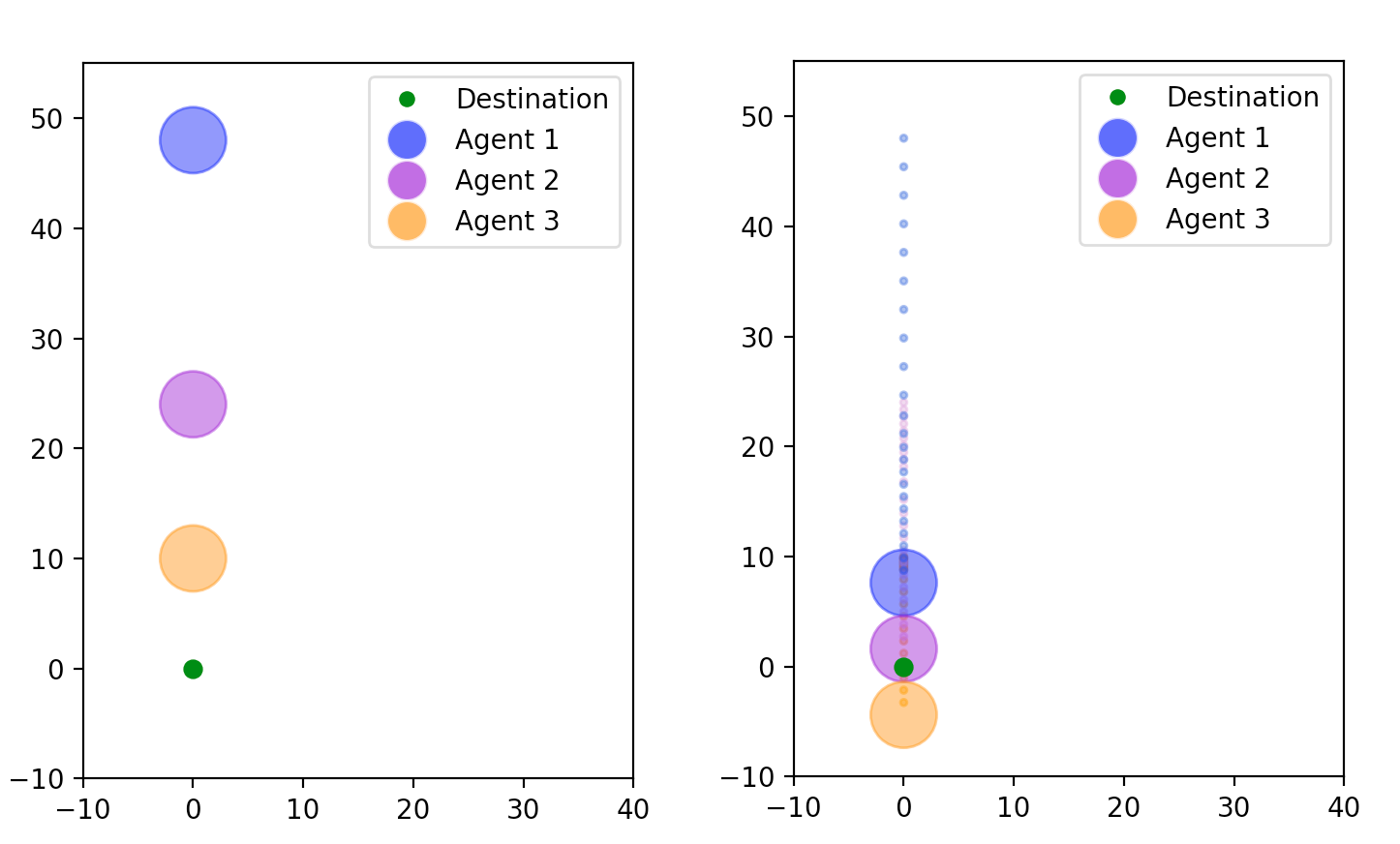
Figure 19: Illustration for Example 4.5 at $t=0$ and $t=T$

Example 4.5

Consider the controlled crowd motion problem with the following data (see Figure 19):

$$\begin{cases}{\bf x}^{des}=(0,0),\;{\bf x}_{1}^{0}=(0,48),\;{\bf x}_{2}^{0}=(0,24),\;{\bf x}_{3}^{0}=(0,10)\\ T=6,\;L_{1}=L_{2}=L_{3}=3.\end{cases}$$

The performances of the agents are computed in the below table.

$\tau$	$\overline{a}_{1}$	$\overline{a}_{2}$	$\overline{a}_{3}$	$t^{f}_{12}$	$t^{f}_{23}$	$J[\overline{x},\overline{a}]$
1.0	1.306309	0.653154	0.272148	2.296547	2.796989	60.465
2.0	1.291812	0.645906	0.269128	2.322319	2.828377	84.660
3.0	1.277315	0.638658	0.266107	2.348676	2.860477	108.585
4.0	1.262819	0.631409	0.263087	2.375638	2.893314	132.240
5.0	1.248322	0.624161	0.260067	2.403226	2.926914	155.625
6.0	1.233825	0.616913	0.257047	2.431462	2.961303	178.740
7.0	1.219329	0.609664	0.254027	2.460370	2.996510	201.585
8.0	1.204832	0.602416	0.251007	2.489973	3.032564	224.160
9.0	1.190336	0.595168	0.247987	2.520298	3.069497	246.465
10.0	1.175839	0.587919	0.244966	2.551370	3.107340	268.500

In this case agents 1 and 2 are in contact first as $t^{f}_{12}<t^{f}_{23}$.

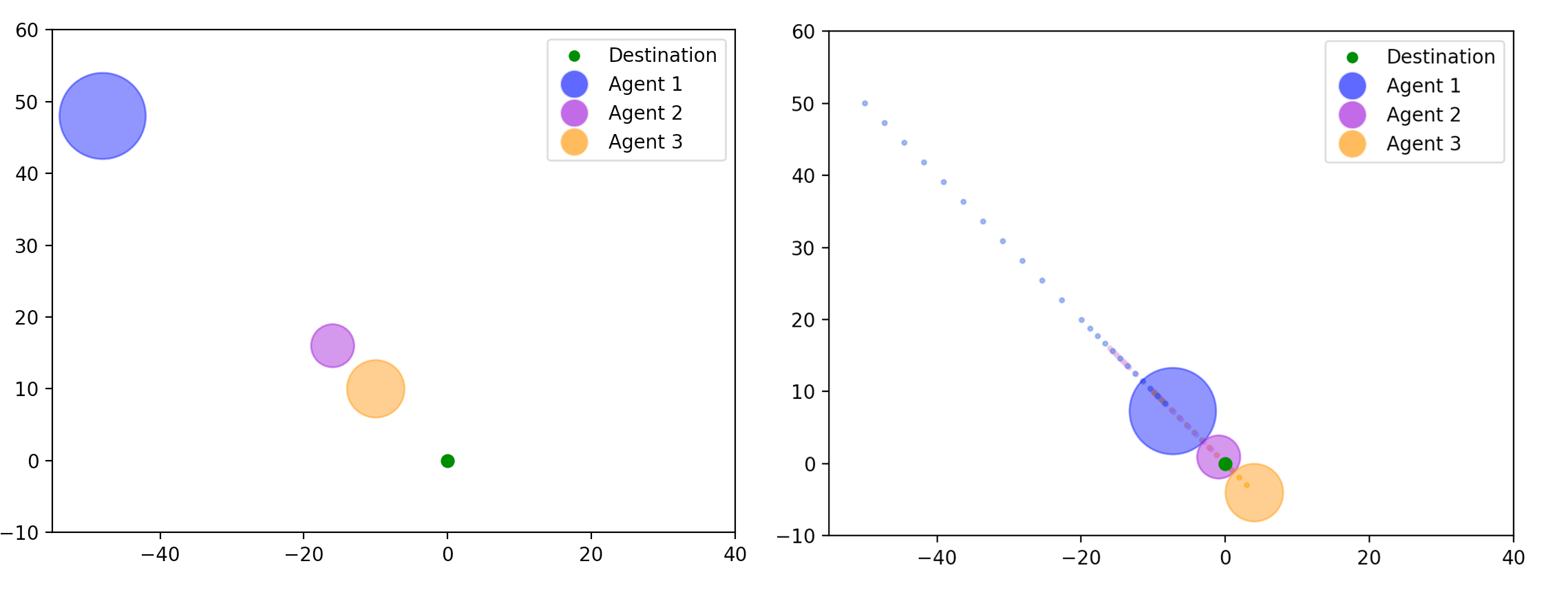
Figure 20: Illustration for Example 4.6 at $t=0$ and $t=T$

Example 4.6

Consider the controlled crowd motion problem with the following data (see Figure 20):

$$\begin{cases}{\bf x}^{des}=(0,0),\;{\bf x}_{1}^{0}=(-50,50),\;{\bf x}_{2}^{0}=(-16,16),\;{\bf x}_{3}^{0}=(-10,10)\\ T=6,\;L_{1}=6,\;L_{2}=3,\;L_{3}=4.\end{cases}$$

We can calculate the optimal velocities, the contact times and the optimal costs with respect to $\tau$ in the following table.

$\tau$	$\overline{a}_{1}$	$\overline{a}_{2}$	$\overline{a}_{3}$	$t^{f}_{12}$	$t^{f}_{23}$	$J[\overline{x},\overline{a}]$
1.0	1.322654	0.423249	0.264531	2.750828	1.527018	87.065833
2.0	1.314776	0.420728	0.262955	2.767311	1.536168	109.663333
3.0	1.306898	0.418207	0.261380	2.783992	1.545428	132.125833
4.0	1.299020	0.415686	0.259804	2.800877	1.554801	154.453333
5.0	1.291141	0.413165	0.258228	2.817967	1.564288	176.645833
6.0	1.283263	0.410644	0.256653	2.835267	1.573891	198.703333
7.0	1.275385	0.408123	0.255077	2.852780	1.583613	220.625833
8.0	1.267507	0.405602	0.253501	2.870512	1.593456	242.413333
9.0	1.259629	0.403081	0.251926	2.888465	1.603422	264.065833
10.0	1.251751	0.400560	0.250350	2.906644	1.613513	285.583333

In this case agents 2 and 3 are in contact first as $t^{f}_{12}>t^{f}_{23}$.

Remark 4.7

If two of the three agents, e.g. $\overline{\bf x}_{1}$ and $\overline{\bf x}_{2}$, have contact initially, they can be regarded to only agent denoted by $\overline{\bf x}_{12}\colon=\frac{1}{2}(\overline{\bf x}_{1}+\overline{\bf x}_{2})$ and hence can be identified with an elastic disk with the center $\overline{\bf x}_{12}$ and radius $L_{12}=L_{1}+L_{2}$. As a result, the motion models with three agents can be reduced to the one with two agents. In this particular case, agent 2 can be considered the leader and agent 1 will follow him/her by copying his/her action. The motion models with more than three agents are too more complicated but can be reduced to the models with three agents by assigning all agents to three different groups in an appropriate way.

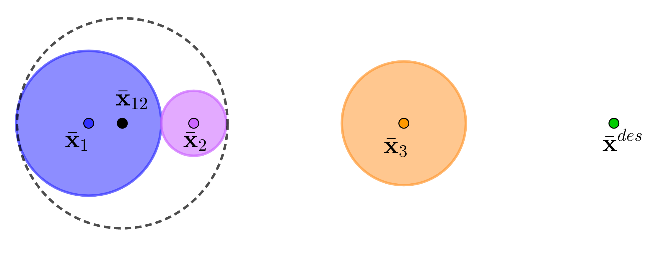
Figure 21: Illustration for Remark 4.7

5 Concluding Remarks and Future Research

Several optimal control problems for the crowd motion models of our interests are studied and their necessary optimality conditions are obtained in this paper. These effective conditions together with the constructive algorithms allow us to solve the dynamic optimization problems associated with the single agent and one obstacle and the problems associated with two and three agents in corridors in a systematic way. The framework of our models can be applied to solve some practical models in real-world situations. For example, the agent (a robot or a driver) may need a smart device to compute an optimal obstacle-free path $\pi$ from some starting point to the destination such that for any point $p$ on $\pi$, the point $q$ on $\pi$ that is distance $L$ away from $p$ is seen by $p$, as is all of the path $\pi$ between $p$ and $q$. In particular, the agent moving along the path $\pi$ is always able to look ahead a distance $L$ to see whether the pathway is clear of debris or one may think of driving a road and wanting to be able to see if there are rocks, limbs, children in the roadway so that one has sufficient amount of time.

In our future research, we intend to explore our study of the controlled planar crowd motion model for two or more participants with general data sets. The cases when two agents are not inline with the destination (in general planar settings) are much more involved and have not been studied fully in this paper and even in [13]. Note that in such cases, the relation (4.10) which plays an essential role in computing optimal solutions is no longer valid due to the fact that two agents have different directions towards the destination. The challenging issue is how to make use of (4.8) and (4.9) derived from the necessary optimality conditions in Theorem 4.1 in order to deduce some useful relation between agents $i$ and $j$ that is similar to (4.10). In case when agents $i$ and $j$ are collinear with the destination, we can obtain that $\alpha_{i}(t^{f}_{ij})=\alpha_{j}(t^{f}_{ij})=\alpha_{ij}(t^{f}_{ij})$. This is, however, not the case when they are not inline and hence such a relation between the directions $\alpha_{i}(t^{f}_{ij}),\alpha_{j}(t^{f}_{ij})$, and $\alpha_{ij}(t^{f}_{ij})$ is missing which complicates the problems under consideration. Using the results from [13, Section 4] together with the effective necessary optimality conditions in Theorem 4.1 may allow us to address such challenging issues and hence to solve the dynamic optimization problems for the planar crowd motion models successfully. Our current work in this paper and in [7, 12, 13] only considered the simplest choice for the desired (spontaneous) velocity of all agents. They have the same behavior: they would like to reach the destination by following the shortest path. Thus, the uncontrolled desired velocity follows the gradient descent of the distance function between the agent and the destination, i.e.,

$${\bf U}({\bf x}):=-s\nabla D^{des}({\bf x})=-s\dfrac{{\bf x}-{\bf x}^{des}}{\left\|{\bf x}-{\bf x}^{des}\right\|}$$

where $s$ denotes the speed of the agent. Motivated from [40] we will consider more practical choices for the desired velocity: the agents can elaborate complex strategies to escape. For instance, in case of congestion, they may decelerate or try to avoid the jam, instead of keeping pushing ineffectively; see [40] for more details. In addition, we also intend to continue our study of solving optimization of controlled crowd motions with multiple agents and obstacles by developing numerical algorithms based on the necessary optimality conditions in Theorem 4.1. Furthermore, our results in this paper can be developed to investigate a new challenging class of bilevel optimal sweeping control problems arising in many real-world situations in which the systems of objects subject to sweeping control have an heterogeneous nature; for example, managing the motion of structured crowds organized in groups, operating teams of drones providing complementary services in a shared confined space. At the upper level of this bilevel framework, each agent of groups of participants seeks an optimal strategy to reach the destination in the minimum time while not overlapping with other groups. At the lower level, each subgroup will follow its own agent with minimum effort while keeping a safe distance with agent and with other members in the same group. Moreover, we may consider the three-dimensional controlled crowd motion model and develop innovative algorithms to solve future problems of maintaining air traffic; for instance, the navigation of a swarm of drones which can intercommunicate. We refer the reader to the excellent survey [36] for the swarm robotic behaviors and current applications. The necessity to develop such algorithms arises from the problems associated with escalating ground traffic congestion and with maintaining the road infrastructure; see [2]. In recent years, there have been researchers working on sustainable aerial transportation systems such as drones and hybrid flying cars. Therefore, it is essential to design efficient obstacle-avoiding algorithms to navigate these unmanned aerial vehicles.

6 Algorithms

This section presents all the algorithms used in our paper.

   1 Optimal control

 

1:procedure optimal a($T$, ${\bf x}^{0}$, ${\bf x}^{obs}$, ${\bf x}^{des}$, $L$, $r$, $s$, $\tau$)

2:     Compute $\mu=\arg\min\{d(\mu):\mu\mbox{ satisfies }\eqref{mu}\}$

3:     Compute $\overline{\bf x}(t_{f})=(1-\mu){\bf x}^{0}+\mu{\bf x}^{des}$

4:     Compute $\overline{\bf x}(t_{l})=\arg\min\left\{\|{\bf x}-\overline{\bf x}(t_{f})\|:\;{\bf x}\mbox{ satisfies }\eqref{e13}\right\}$

5:     Minimize the cost functional $J[\overline{\bf x},\overline{a}]$ in (3.18)

6:end procedure

 

   2 Optimal control for the crowd motion models with two agents in a corridor

 

1:procedure optimal a($T$, ${\bf x}^{0}$, ${\bf x}^{des}$, $L_{1}$, $L_{2}$, $\tau$)

2:     Compute $s_{i}=\dfrac{\|{\bf x}^{des}-\overline{\bf x}_{i}(0)\|}{T}$

3:     if $\overline{\bf x}_{21}(0)-\overline{\bf x}_{11}(0)=L_{1}+L_{2}$ then

4:         minimize the cost functional $J[\overline{\bf x},\overline{a}]$ in (4.19)

5:     else

6:         minimize the cost functional $J[\overline{\bf x},\overline{a}]$ in (4.22) (there is no contact)

7:         compute $\eta_{12}(t^{f}_{12})$ in terms of $\overline{a}_{2}$ using (4.14)

8:         compute $\Lambda_{12}$ and $t^{f}_{12}$ in terms of $\overline{a}_{2}$ using (4.16)

9:         compute ${\bf x}_{1}(t),{\bf x}_{2}(t)$ in terms of $\overline{a}_{2}$ using (4.15)

10:         minimize the cost functional $J[\overline{\bf x},\overline{a}]$ in (4.17)

11:         compare the minimum cost in (4.17) and (4.22)

12:     end if

13:     compute $\overline{a}_{1}=\dfrac{s_{1}}{s_{2}}\overline{a}_{2}$

14:end procedure

 

   3 Optimal control for the crowd motion models with three agents in a corridor

 

1:procedure optimal a($T$, ${\bf x}^{0}$, ${\bf x}^{des}$, $L_{1}$, $L_{2}$, $L_{3}$, $\tau$)

2:     compute $s_{i}=\dfrac{\|{\bf x}^{des}-\overline{\bf x}_{i}(0)\|}{T}$

3:     compute $\Lambda=\dfrac{\Lambda_{12}}{s_{1}^{2}-s_{2}^{2}}-\dfrac{\Lambda_{23}}{s_{2}^{2}-s_{3}^{2}}$

4:     if $\Lambda<0$ then

5:         $t^{f}_{12}<t^{f}_{123}=t^{f}_{23}$

6:         compute $\eta_{12}(t^{f}_{12}),\eta_{12}(t^{f}_{123}),$ and $\eta_{23}(t^{f}_{123})$ using (4.30) and (4.31)

7:         compute $t^{f}_{123}$ using (4.32)

8:         compute $\overline{\bf x}_{1}(T),\overline{\bf x}_{2}(T),$ and $\overline{\bf x}_{3}(T)$ using (4.33)–(4.35)

9:         minimize the objective function $J[\overline{\bf x},\overline{a}]$ in (4.36)

10:     end if

11:     if $\Lambda>0$ then

12:         $t^{f}_{23}<t^{f}_{123}=t^{f}_{12}$

13:         compute $\eta_{23}(t^{f}_{23}),\eta_{23}(t^{f}_{123}),$ and $\eta_{12}(t^{f}_{123})$ using (4.37) and (4.38)

14:         compute $t^{f}_{123}$ using (4.39)

15:         compute $\overline{\bf x}_{1}(T),\overline{\bf x}_{2}(T),$ and $\overline{\bf x}_{3}(T)$ using (4.40)–(4.42)

16:         minimize the objective function $J[\overline{\bf x},\overline{a}]$ in (4.36)

17:     end if

18:     if $\Lambda=0$ then

19:         compute $\eta_{12}(t^{f}_{123})$ and $\eta_{23}(t^{f}_{123})$ using (4.43) and (4.44)

20:         minimize the objective function $J[\overline{\bf x},\overline{a}]$ in (4.36)

21:     end if

22:end procedure

 

Acknowledgments. The authors are indebted to Boris Mordukhovich for his helpful remarks and discussions on the original presentation.

References

- [1] L. Adam and J. V. Outrata, On optimal control of a sweeping process coupled with an ordinary differential equation, Discrete Contin. Dyn. Syst. Ser. B, 19 (2014), 2709–2738.
- [2] S. S. Ahmed , K. F. Hulme, G. Fountas, U. Eker, I. V. Benedyk, S. E. Still, and P. C. Anastasopoulos, The flying car – challenges and strategies toward future adoption, Frontiers in Built Environment, 6 (2020).
- [3] C. E. Arroud and G. Colombo, A maximum principle of the controlled sweeping process, Set-Valued Var. Anal., 26 (2018), 607–629.
- [4] A. Canino, On -convex sets and geodesics, J. Diff. Eqs., 75 (1988), 118–0157.
- [5] T. H. Cao, N. T. Khalil, B. S. Mordukhovich, D. Nguyen, and F. L. Pereira, Crowd motion paradigm modeled by a bilevel sweeping control problem, IEEE Control Systems Letters, 6 (2022), 385–390.
- [6] T. H. Cao, N. T. Khalil, B. S. Mordukhovich, D. Nguyen, T. Nguyen, and F. L. Pereira, Optimization of controlled free-time sweeping process with applications to marine surface vehicle modeling, IEEE Control Systems Letters, 6 (2022), 782–787.
- [7] T. H. Cao, B. S. Mordukhovich, D. Nguyen, and T. Nguyen, Applications of controlled sweeping processes to nonlinear crowd motion models with obstacles, IEEE Control Systems Letters , 6 (2022), 740–745.
- [8] T. H. Cao, G. Colombo, B. S. Mordukhovich, and D. Nguyen, Optimization of fully controlled sweeping process, J. Diff. Eqs, 295 (2021), 138–186.
- [9] T. H. Cao, G. Colombo, B. S. Mordukhovich, and D. Nguyen, Optimization and discrete approximation of sweeping process with controlled moving sets and perturbations, J. Diff. Eqs., 274 (2021), 461–509 .
- [10] T. H. Cao and B. S. Mordukhovich, Optimal control of a perturbed sweeping process via discrete approximations. Discrete Contin. Dyn. Syst.-Ser. B, 21 (2016), 3331–3358.
- [11] T. H. Cao and B. S. Mordukhovich, Optimality conditions for a controlled sweeping process with applications to the crowd motion model, Discrete Contin. Dyn. Syst.-Ser. B, 21 (2017), 267–306.
- [12] T. H. Cao and B. S. Mordukhovich, Optimal control of a nonconvex perturbed sweeping process, J. Diff. Eqs., 266 (2019), 100–1050.
- [13] T. H. Cao and B. S. Mordukhovich, Applications of the controlled sweeping process to optimal control of the planar crowd motion model, Discrete Contin. Dyn. Syst., Ser. B, 24 (2019), 4191–4216.
- [14] C. Castaing, M. D. P. Monteiro Marques and P. Raynaud de Fitte, Some problems in optimal control governed by the sweeping process, J. Nonlinear Convex Anal., 15 (2014), 1043–1070.
- [15] F. H. Clarke, Necessary conditions in dynamic optimization, Mem. Amer. Math. Soc., 173 (2005), No. 816.
- [16] G. Colombo, B. S. Mordukhovich and D. Nguyen, Optimal control of sweeping processes in robotics and traffic flow models, J. Optim. Theory Appl., 182 (2019), 439–472.
- [17] G. Colombo, B. S. Mordukhovich and D. Nguyen, Optimization of a perturbed sweeping process by discontinuous control, SIAM J. Control Optim., 58 (2020), 2678–2709.
- [18] G. Colombo, R. Henrion, N. D. Hoang and B. S. Mordukhovich, Optimal control of the sweeping process. Dyn. Contin. Discrete Impuls. Syst.–Ser. B, 19 (2012), 117–159.
- [19] G. Colombo, R. Henrion, N. D. Hoang and B. S. Mordukhovich, Optimal control of the sweeping process over polyhedral controlled sets. J. Diff. Eqs., 260 (2016), 3397–3447.
- [20] G. Colombo and L. Thibault, Prox-regular sets and applications, In Y. Gao and D. Motreanu, editors, Handbook of Nonconvex Analysis, pages 99–182. International Press, 2010.
- [21] M. d. R. de Pinho, M. M. A. Ferreira and G. V. Smirnov. Optimal control involving sweeping processes. Set-Valued Var. Anal., to appear.
- [22] T. Donchev, E. Farkhi, and B. S. Mordukhovich, Discrete approximations, relaxation, and optimization of one-sided Lipschitzian differential inclusions in Hilbert spaces. J. Diff. Eqs., 243 (2007), 301–328.
- [23] J. F. Edmond and L. Thibault, Relaxation of an optimal control problem involving a perturbed sweeping process. Math. Program., 104 (2005), 347–373.
- [24] N. T. Khalil and F. L. Pereira, A framework for the control of bilevel sweeping processes, IEEE 58th Conference on Decision and Control (CDC), 2019.
- [25] N. T. Khalil and F. L. Pereira, A Maximum Principle for a time-optimal bi-level sweeping control problem, IFAC-PapersOnLine, 53 (2020), 6831–6836.
- [26] M. d. R. de Pinho, M. M. A. Ferreira and G. V. Smirnov, Optimal control with sweeping processes: numerical method, J. Optim. Theory Appl., 185 (2020), 845–858.
- [27] M. d. R. de Pinho, M. M. A. Ferreira and G. V. Smirnov, Optimal control involving sweeping processes, Set-Valued Var. Anal., 27 (2019), 523–548.
- [28] B. Maury and J. Venel, A discrete model for crowd motion, ESAIM: M2AN, 45 (2011), 145–168.
- [29] B. S. Mordukhovich, Optimal control of differential inclusions, I: Lipschitzian case, Bull. Irkutsk State Univ. Ser. Math., 30 (2019), 39–50.
- [30] B. S. Mordukhovich, Optimal control of differential inclusions, II: Sweeping, Bull. Irkutsk State Univ., Ser. Math., 31 (2020), 62–77.
- [31] B. S. Mordukhovich, Discrete approximations and refined Euler-Lagrange conditions for differential inclusions, SIAM J. Control Optim. 33 (1995), 882–915.
- [32] B. S. Mordukhovich, Variational Analysis and Generalized Differentiation, I: Basic Theory, II: Applications, Springer, Berlin, 2006.
- [33] J. J. Moreau, On Unilateral Constraints, Friction and Plasticity, in: G. Capriz and G. Stampacchia (Eds.), New Variational Techniques in Mathematical Physics, Proceedings of C.I.M.E. Summer Schools, Cremonese, Rome, 1974, 173–322.
- [34] C. Nour and V. Zeidan, Optimal control of nonconvex sweeping processes with separable endpoints: nonsmooth maximum principle for local minimizers, J. Diff. Eqs., 318 (2022), 113–168.
- [35] C. Nour and V. Zeidan, Numerical solution for a controlled nonconvex sweeping process, IEEE Control Systems Letters, 6 (2022), 1190–1195.
- [36] M. Schranz, M. Umlauft, M. Sende, and W. Elmenreich, Swarm robotic behaviors and current applications, Frontiers in Robotics and AI, 7 (2020).
- [37] A. A. Tolstonogov, Sweeping process with unbounded nonconvex perturbation, Nonlinear Anal., 108 (2014), 291–301.
- [38] A. A. Tolstonogov, Control sweeping processes, J. Convex Anal., 23 (2016), 1099–1123.
- [39] J. Venel, A numerical scheme for a class of sweeping process. Numerische Mathematik, 118 (2011), 451–484.
- [40] J. Venel, Integrating strategies in numerical modeling of crowd motion, Pedestrian and Evacuation Dynamics ’08, Springer 641–646 (2010).
- [41] R. B. Vinter, Optimal Control, Birkhäuser Boston, MA, 2000.
- [42] V. Zeidan, C. Nour, and H. Saoud, A nonsmooth maximum principle for a controlled nonconvex sweeping process, J. Diff. Eqs., 269 (2020), 9531–9582.