Path integral in position-deformed Heisenberg algebra with strong quantum gravitational measurement

Abstract

Position-deformed Heisenberg algebra with maximal length uncertainty has recently been proven to induce strong quantum gravitational fields at the Planck scale (2022 J. Phys. A: Math. Theor. 55 105303). In the present study, we use the position space representation on the one hand and the Fourier transform and its inverse representations on the other to construct propagators of path integrals within this deformed algebra. The propagators and the corresponding actions of a free particle and a simple harmonic oscillator are discussed as examples. Since the effects of quantum gravity are strong in this Euclidean space, we show that the actions which describe the classical trajectories of both systems are bounded by the ordinary ones of classical mechanics. This indicates that quantum gravity bends the paths of particles, allowing them to travel quickly from one point to another. It is numerically observed by the decrease in values of classical actions as one increases the quantum gravitational effects.

1 Introduction

Due to a constant search for a consistent theory of quantum gravity, the deformation of Heisenberg algebra with minimal measurable uncertainty length has been one of the most intense fields in the last two decades [2, 3, 4, 5, 6, 7, 8, 9, 10, 11, 12, 13]. It is widely known that the existence of this minimal uncertainty length presents the issue of high energy requirements that are beyond the scope of any experimental feasibility. To circumvent this requirement, one of us recently has proposed a position-deformed Heisenberg algebra [14] in two dimensions (2D) that introduces the simultaneous existence of minimal and maximal length uncertainties. The emergence of this maximal length demonstrated strong quantum gravitational effects in this space and predicted the detection of low-energy gravity particles [1]. In continuation of this work, we construct the position space representation describing this maximal length, as well as the corresponding Fourier transform and its inverse representations. We derive the propagators of path integrals based on these different representations by following the work done in minimal length scenarios [15, 16, 17, 18].

The Hamiltonian’s principle of least action is used to generate the equations of motion. We compute the propagators and actions of a free particle and a simple harmonic oscillator as applications. Since the quantum gravity is strongly measured in this space [1], we show that the classical trajectories of particles described by their actions are deformed, allowing particles to take the shortest path between two points in the minimum time. This result strengthens the claim that the recently proposed position-deformed algebra [1] induces strong quantum gravitational fields with features close to those of classical ones of general relativity.

This paper is outlined as follows: in section 2, we establish Hilbert space representations of wave functions associated with this deformed algebra. In section 3, we construct the path integrals in these wave function representations and deduce the corresponding quantum propagators and classical actions. As examples, we compute the propagators and the actions for some simple models such as the free particle and the harmonic oscillators. In the last section, we present our conclusion.

2 Position deformed Heisenberg algebra with maximal length

Let $\mathcal{H}=\mathcal{L}^{2}(\mathbb{R})$ be the Hilbert space of square integrable functions. The Hermitian operators $\hat{x}$ and $\hat{p}$ that act in this space satisfy the condition

$${[\hat{x},\hat{p}]}=i\hbar\mathbb{I}.$$ (1)

The corresponding Heisenberg uncertainty principle is given by

$$\Delta x\Delta p\geq\frac{\hbar}{2}.$$ (2)

Let $\{|x\rangle\}\in\mathcal{H}$ be the complete position basis vectors. The action operators in equation (1) on this basis vector reads as follows

$$\hat{x}|x\rangle=x|x\rangle\quad\mbox{and}\quad\hat{p}|x\rangle=-i\hbar\frac{d}{dx}|x\rangle,\quad x\in\mathbb{R}.$$ (3)

The completeness and orthogonality relations are given by

$$\langle x^{\prime}|x\rangle=\delta(x-x^{\prime}),\quad\int_{-\infty}^{+\infty}dx|x\rangle\langle x|=\mathbb{I}.$$ (4)

Another useful choice of basis vectors is the momentum vector $\{|p\rangle\}\in\mathcal{H}$ defined by taking Fourier transforms

$$|p\rangle=\int_{-\infty}^{+\infty}dxe^{ipx}|x\rangle\quad\mbox{with}\quad p\in\mathbb{R}$$ (5)

and its inverse is defined as follows

$$|x\rangle=\int_{-\infty}^{+\infty}\frac{dp}{2\pi}e^{-ipx}|p\rangle.$$ (6)

The inner product and completeness relations are given by

$$\langle p^{\prime}|p\rangle=\delta(p-p^{\prime}),\quad\int_{-\infty}^{+\infty}\frac{dp}{2\pi}|p\rangle\langle p|=\mathbb{I}.$$ (7)

The action of the operators in (1) on the vector $|p\rangle$ is given by

$$\hat{p}|p\rangle=\int_{-\infty}^{+\infty}dx\left(-i\frac{d}{dx}e^{ipx}\right)|x\rangle=p|p\rangle,\quad\hat{x}|p\rangle=\int_{-\infty}^{+\infty}dx\left(i\hbar\frac{d}{dp}e^{ipx}\right)|x\rangle=i\hbar\frac{d}{dp}|p\rangle.$$ (8)

Let us consider new operators $\hat{X}$ and $\hat{P}$ on $\mathcal{H}$. We define them by

$$\hat{X}=\hat{x},\quad\hat{P}=(\mathbb{I}-\tau\hat{x}+\tau^{2}\hat{x}^{2})\hat{p}.$$ (9)

They satisfy the following relation [1]

$${[\hat{X},\hat{P}]}=i\hbar(\mathbb{I}-\tau\hat{X}+\tau^{2}\hat{X}^{2}),$$ (10)

where $\tau\in(0,1)$ is the generalized uncertainty principle parameter related to quantum gravitational effects in this space which describes the Planck scale [2, 3]. Obviously by taking $\tau\rightarrow 0$, we recover the algebra (1). The action of these operators on the following unit basis vectors $\{|x\rangle\}$ and $\{|p\rangle\}$ reads as follows

$$\hat{X}|x\rangle = x|x\rangle\quad\mbox{and}\quad\hat{P}|x\rangle=-i\hbar(1-\tau x+\tau^{2}x^{2})\partial_{x}|x\rangle,\quad x\in\mathbb{R}.$$ (11)

$$\hat{X}|p\rangle = i\hbar\partial_{p}|x\rangle\quad\mbox{and}\quad\hat{P}|p\rangle=(1-i\tau\hbar\partial_{p}-\tau^{2}\hbar^{2}\partial_{p}^{2})p|p\rangle,\quad p\in\mathbb{R}.$$ (12)

Let us consider an arbitrary vector $|\phi\rangle\in\mathcal{H}$, the projection of this vector on the unit vectors $\{|x\rangle\}$ and $\{|p\rangle\}$ generates the functions $\phi(x)$ and $\phi(p)$. As a result, we can write the above equations as follows

$$\hat{X}\phi(x) = x\phi(x)\quad\mbox{and}\quad\hat{P}\phi(x)=-i\hbar(1-\tau x+\tau^{2}x^{2})\partial_{x}\phi(x),$$ (13)

$$\hat{X}\phi(p) = i\hbar\partial_{p}\phi(p)\quad\mbox{and}\quad\hat{P}\phi(p)=(1-i\tau\hbar\partial_{p}-\tau^{2}\hbar^{2}\partial_{p}^{2})p\phi(p).$$ (14)

An interesting feature can be observed from the commutation relation (10) through the following uncertainty relation:

$$\Delta X\Delta P\geq\frac{\hbar}{2}\left(1-\tau\langle\hat{X}\rangle+\tau^{2}\langle\hat{X}^{2}\rangle\right).$$ (15)

Using the relation $\langle\hat{X}^{2}\rangle=(\Delta X)^{2}+\langle\hat{X}\rangle^{2}$, the equation (15) can be rewritten as a second order equation for $\Delta X$

$$\Delta X^{2}-\frac{2}{\hbar\tau^{2}}\Delta P\Delta X+\langle\hat{X}\rangle^{2}-\frac{1}{\tau}\langle\hat{X}\rangle+\frac{1}{\tau^{2}}\leq 0.$$ (16)

The solutions for $\Delta X$ are given by

$$\Delta X=\frac{\Delta P}{\hbar\tau^{2}}\pm\sqrt{\left(\frac{\Delta P}{\hbar\tau^{2}}\right)^{2}-\frac{\langle\hat{X}\rangle}{\tau}\left(\tau\langle\hat{X}\rangle-1\right)-\frac{1}{\tau^{2}}}.$$ (17)

This equation leads to the absolute minimal uncertainty $\Delta P_{min}$ in $P$-direction and the absolute maximal uncertainty $\Delta X_{max}$ in $X$-direction when $\langle\hat{X}\rangle=0$ [14]

$$\quad\Delta X_{max}=\frac{1}{\tau}\quad\mbox{and}\quad\Delta P_{min}=\hbar\tau.$$ (18)

It is well known that [2], the existence of minimal uncertainty raises the question of the loss of representation i.e., the space is inevitably bounded by minimal quantity beyond which any further localization of particles is not possible. In the presente situation, the minimal momentum $\Delta P_{min}$ leads to a loss of $\phi(p)$-representation and a maximal $\phi(x)$-representation. Thus, the corresponding representation of operators are given by

$$\hat{X}\phi(x) = x\phi(x)\quad\mbox{and}\quad\hat{P}\phi(x)=-i\hbar D_{x}\phi(x),$$ (19)

where $D_{x}=(1-\tau x+\tau^{2}x^{2})\partial_{x}$ is a deformed derivative. Using this equation (19), one can recover the algebra (10).

As one can see from the representation of operators in equation (9) or in equation (19), the position operator $\hat{X}$ is Hermitian while the momentum operator $\hat{P}$ is not

$$\hat{X}^{\dagger}=\hat{X}\quad\mbox{and}\quad\hat{P}^{\dagger}=\hat{P}+i\hbar\tau(\mathbb{I}-2\tau\hat{X})\implies\hat{P}^{\dagger}\neq\hat{P}.$$ (20)

Thus, the Hermicity requirement of the momentum operator leads to the introduction of the following completeness relation [1]

$$\int_{-\infty}^{+\infty}\frac{dx}{1-\tau x+\tau^{2}x^{2}}|x\rangle\langle x|=\mathbb{I}.$$ (21)

To proof the Hermicity of this operator, we have to restrict the action of $\hat{P}$ in a physical dense subset, $\mathcal{D}(\hat{P})\subset\mathcal{H}$, which we shall call the domain of $\hat{P}$ defined as follows

$$\mathcal{D}(\hat{P})=\{\varphi,-i\hbar D_{x}\varphi\in\mathcal{L}^{2}(-\infty,+\infty),\,\,\lim_{x\rightarrow\pm\infty}\varphi(x)=0\}.$$ (22)

The restriction to dense subset guarantees the existence of the adjoint operator $\hat{P}^{\dagger}$, a necessary condition for one to obtain the Hermicity of this operator. The adjoint domain is defined by

$$\mathcal{D}(\hat{P}^{\dagger})=\{\xi,-i\hbar D_{x}\xi\in\mathcal{L}^{2}(-\infty,+\infty)\}.$$ (23)

Thus, we may write $\mathcal{D}(\hat{P})\subset\mathcal{D}(\hat{P}^{\dagger})$, which means that the domain of $\hat{P}$ is a proper subset of the domain of its adjoint $\hat{P}^{\dagger}$. To show the Hermicity of the oparator $\hat{P}$, we consider the functional $B(\xi,\varphi)$ defined by

$$B(\xi,\varphi):=\langle\xi|\hat{P}\varphi\rangle-\langle\hat{P}^{\dagger}\xi|\varphi\rangle.$$ (24)

Using the relation (21) and by a straightforward computation of this functional, we have

$$B(\xi,\varphi) = \int_{-\infty}^{+\infty}\frac{dx}{1-\tau x+\tau^{2}x^{2}}\left[\xi^{*}(x)\left(-i\hbar D_{x}\varphi(x)\right)-\left(-i\hbar D_{x}\xi(x)\right)^{*}\varphi(x)\right]$$ (25)

$$= -i\hbar\int_{-\infty}^{+\infty}d\left(\xi^{*}(x)\varphi(x)\right)=-i\hbar\left[\xi^{*}(x)\varphi(x)\right]_{-\infty}^{+\infty}.$$ (26)

Since $\lim_{x\rightarrow\pm\infty}\varphi(x)=0$, and $\xi(x)$ can reach any arbitrary value at the boundaries. This lead to the vanishing of $B(\xi,\varphi)$ i.e., $B(\xi,\varphi)=0$. Consequently, the operator $\hat{P}$ is a Hermitian in $\mathcal{D}(\hat{P})$ such that

$$\langle\xi|\hat{P}\varphi\rangle=\langle\hat{P}^{\dagger}\xi|\varphi\rangle\implies\hat{P}=\hat{P}^{\dagger}.$$ (27)

Despite the fact that the momentum is Hermitian, it is not always a self-adjoint operator because its domain includes the domain of $\hat{P}^{\dagger}$. It could have none, or it could have an infinite number of self-adjoint extensions. Note that, as rule in quantum mechanics, the operators that act on square integrable functions are essentially self-adjoint. There are exceptions to the rule. This is because the basic quantization requirement that operators whose expectation values are real do not strictly require these operators be self-adjoint. Indeed, the Hermicity result (27) is a sufficient condition to ensure that all expectation values of the momentum operator are real. Moreover, using the completeness relation (21), the scalar product between two states $|\Psi\rangle$ and $|\Phi\rangle$ and the orthogonality of eigenstates become

$$\langle\Psi|\Phi\rangle = \int_{-\infty}^{+\infty}\frac{dx}{1-\tau x+\tau^{2}x^{2}}\Psi^{*}(x)\Phi(x),$$ (28)

$$\langle x|x^{\prime}\rangle = (1-\tau x+\tau^{2}x^{2})\delta(x-x^{\prime}).$$ (29)

To construct a Hilbert space representation that describes the maximal length and the minimal momentum uncertainties, one has to solve the eigenvalue problem

$$-i\hbar D_{x}\phi_{\rho}(x)=\rho\phi_{\rho}(x),\quad\quad\rho\in\mathbb{R}^{*}.$$ (30)

The solution of this equation is given by

$$\phi_{\rho}(x)=A\exp\left(i\frac{2\rho}{\tau\hbar\sqrt{3}}\left[\arctan\left(\frac{2\tau x-1}{\sqrt{3}}\right)+\frac{\pi}{6}\right]\right),$$ (31)

where $A$ is an abritrary constant. Then by normalization, $\langle\phi_{\rho}|\phi_{\rho}\rangle=1$, we have

$$A = \sqrt{\frac{\tau\sqrt{3}}{2\pi}}.$$ (32)

Substituting this equation (32) into the equation (31) gives

$$\phi_{\rho}(x) = \sqrt{\frac{\tau\sqrt{3}}{2\pi}}\exp\left(i\frac{2\rho}{\tau\hbar\sqrt{3}}\left[\arctan\left(\frac{2\tau x-1}{\sqrt{3}}\right)+\frac{\pi}{6}\right]\right).$$ (33)

This wave function describes simultaneously the maximal length and the minimal momentum uncertainties. Furthermore, using the relations (33) and (29), we can defined a new identity operator as follows

$$\int_{-\infty}^{+\infty}\frac{d\rho}{\tau\hbar\sqrt{3}}d\rho|\rho\rangle\langle\rho|=\mathbb{I}.$$ (34)

This identity operator (34) will play the role of the completeness relation of the momentum eigenstates in the derivation of the path-integral.

By projecting an arbitrary state $|\psi\rangle$ onto this localized states $|\phi_{\rho}\rangle$ one can obtain the quasi-momentum representation, that is

$$\psi(\rho)=\langle\phi_{\rho}|\psi\rangle=\sqrt{\frac{\tau\sqrt{3}}{2\pi}}\int_{-\infty}^{+\infty}\frac{dx\psi(x)}{1-\tau x+\tau^{2}x^{2}}e^{-i\frac{2\rho}{\tau\hbar\sqrt{3}}\left[\arctan\left(\frac{2\tau x-1}{\sqrt{3}}\right)+\frac{\pi}{6}\right]}.$$ (35)

This mapping defined the generalized Fourier transform of the representation in equation (33). Its inverse representation is given by

$$\psi(x)=\frac{1}{\hbar\sqrt{2\pi\tau\sqrt{3}}}\int_{-\infty}^{+\infty}d\rho\psi(\rho)e^{i\frac{2\rho}{\tau\hbar\sqrt{3}}\left[\arctan\left(\frac{2\tau x-1}{\sqrt{3}}\right)+\frac{\pi}{6}\right]}.$$ (36)

Moreover from equation (35), we can deduce that

$$\frac{d}{d\rho}e^{-i\frac{2\rho}{\tau\hbar\sqrt{3}}\left[\arctan\left(\frac{2\tau x-1}{\sqrt{3}}\right)+\frac{\pi}{6}\right]} = -i\frac{2}{\tau\hbar\sqrt{3}}\left[\arctan\left(\frac{2\tau x-1}{\sqrt{3}}\right)+\frac{\pi}{6}\right]$$ (38)

$$\times e^{-i\frac{2\rho}{\tau\hbar\sqrt{3}}\left[\arctan\left(\frac{2\tau x-1}{\sqrt{3}}\right)+\frac{\pi}{6}\right]}.$$

This equation is equivalent to

$$i\frac{\tau\hbar\sqrt{3}}{2}\frac{d}{d\rho}=\left[\arctan\left(\frac{2\tau x-1}{\sqrt{3}}\right)+\frac{\pi}{6}\right]=\left[\arctan\left(\frac{2\tau x-1}{\sqrt{3}}\right)+\arctan\left(\frac{1}{\sqrt{3}}\right)\right].$$ (39)

From the following relation [19]

$$\arctan\alpha+\arctan\beta=\arctan\left(\frac{\alpha+\beta}{1-\alpha\beta}\right),\quad\mbox{with}\quad\alpha\beta<1,$$ (40)

we deduce that

$$\tan\left[\arctan\left(\frac{2\tau x-1}{\sqrt{3}}\right)+\arctan\left(\frac{1}{\sqrt{3}}\right)\right]=\frac{\tau x\sqrt{3}}{2-\tau x}.$$ (41)

In equation (39), we can see that the position operator is represented as [10]

$$\hat{X} = \frac{2}{\tau}\frac{\tan\left(i\frac{\tau\hbar\sqrt{3}}{2}\frac{d}{d\rho}\right)}{\sqrt{3}+\tan\left(i\frac{\tau\hbar\sqrt{3}}{2}\frac{d}{d\rho}\right)},$$ (42)

$$\hat{X}\psi(\rho) = \frac{2}{\tau}\frac{\tan\left(i\frac{\tau\hbar\sqrt{3}}{2}\frac{d}{d\rho}\right)}{\sqrt{3}+\tan\left(i\frac{\tau\hbar\sqrt{3}}{2}\frac{d}{d\rho}\right)}\psi(\rho).$$ (43)

From the action of $\hat{P}$ on the quasi representation (36) and using equation (13), we have

$$\hat{P}\psi(\rho)=\rho\psi(\rho).$$ (44)

Note that in the limit $\tau\rightarrow 0$, we recover the corresponding ordinary quantum mechanics results in momentum space (8)

$$\lim_{\tau\rightarrow 0}\hat{X}\psi(\rho)=i\hbar\frac{d}{d\rho}\psi(\rho)\quad\mbox{and}\quad\lim_{\tau\rightarrow 0}\hat{P}\psi(\rho)=\rho\psi(\rho).$$ (45)

3 Path integral and propagator in position-deformed algebra

From the path integrals within this position-deformed Heisenberg algebra, we construct the propagator depending on the position-representation and on the Fourier transform and its inverse representations. We compute propagators and deduce the actions of a free particle and a harmonic oscillator as applications.

3.1 Path integral and propagator in position-space representation

The Hamiltonian operator for a particle with mass $m$ living in one spatial dimension is given by

$$\hat{H}=\frac{\hat{P}^{2}}{2m}+V(\hat{X}),$$ (46)

where V is the potential energy of the system. The time-dependent deformed Schrödinger equation in the position representation is given by

$$\hat{H}|\phi_{\rho}(t)\rangle=-\frac{\hbar^{2}}{2m}D_{x}^{2}|\phi_{\rho}(t)\rangle+V(x)|\phi_{\rho}(t)\rangle=i\hbar\partial_{t}|\phi_{\rho}(t)\rangle.$$ (47)

The time-evolution process is described by

$$|\phi_{\rho}(t)\rangle=e^{-\frac{i}{\hbar}\hat{H}(t-t^{\prime})}|\phi_{\rho}(t^{\prime})\rangle,$$ (48)

Multiplication of $\langle x|$ from the left of the equation (48) gives

$$\phi_{\rho}(x,t)=\int_{-\infty}^{+\infty}\frac{dx^{\prime}}{1-\tau x^{\prime}+\tau^{2}x^{\prime 2}}K(x,t,x^{\prime},t^{\prime})\phi_{\rho}(x^{\prime},t^{\prime})$$ (49)

where $K$ is the kernel in Hamiltonian or the amplitude for a particle to propagate from the state with position $x^{\prime}$ to the state with position $x\,(x>x^{\prime})$ in a time interval $\Delta t=t-t^{\prime}$ [20] and it is defined as

$$K(x,t,x^{\prime},t^{\prime})=\langle x|e^{-\frac{i}{\hbar}\hat{H}(t-t^{\prime})}|x^{\prime}\rangle.$$ (50)

Splitting the interval $t-t^{\prime}$ into N intervals of length $\epsilon=(t_{k}-t_{k-1})/N$ and inserting the completeness relations in (28) and (34), the propagator (52) becomes

$$K(x,t,x^{\prime},t^{\prime}) = \prod_{k=1}^{N-1}\left(\int_{-\infty}^{+\infty}\frac{dx_{k}}{1-\tau x_{k}+\tau^{2}x_{k}^{2}}\right)\prod_{k=1}^{N}\left(\int_{-\infty}^{+\infty}\frac{d\rho_{k}}{\tau\hbar\sqrt{3}}\right)$$ (52)

$$\times\langle x_{k}|\rho_{k}\rangle\langle\rho_{k}|e^{-\frac{i}{\hbar}\epsilon\hat{H}}|x_{k-1}\rangle.$$

Recall that

$$\langle x_{k}|\rho_{k}\rangle = \phi_{\rho_{k}}(x_{k})=\sqrt{\frac{\tau\sqrt{3}}{2\pi}}e^{\left(i\frac{2\rho_{k}}{\tau\hbar\sqrt{3}}\left[\arctan\left(\frac{2\tau x_{k}-1}{\sqrt{3}}\right)+\frac{\pi}{6}\right]\right)},$$ (53)

$$\langle\rho_{k}|e^{-\frac{i}{\hbar}\epsilon\hat{H}}|x_{k-1}\rangle = e^{-\frac{i}{\hbar}\epsilon H(\rho_{k},x_{k-1})}\langle\rho_{k}|x_{k-1}\rangle=e^{-\frac{i}{\hbar}\epsilon H(\rho_{k},x_{k-1})}\phi_{\rho_{k}}^{*}(x_{k-1}).$$ (54)

Substituting these expressions into equation (52) gives

$$K(x,t,x^{\prime},t^{\prime})=\left[\prod_{k=1}^{N-1}\left(\int_{-\infty}^{+\infty}\frac{dx_{k}}{1-\tau x_{k}+\tau^{2}x_{k}^{2}}\right)\right]\left[\prod_{k=1}^{N}\left(\frac{1}{\tau\hbar\sqrt{3}}\int_{-\infty}^{+\infty}d\rho_{k}\right)\right]e^{\frac{i}{\hbar}\epsilon\mathcal{S}_{disc}},$$ (55)

where the discrete action $S_{disc}$ is

$$S_{disc} = \sum_{k=1}^{N-1}\frac{2\rho_{k}}{\tau\sqrt{3}}\left[\frac{\arctan\left(\frac{2\tau x_{k}-1}{\sqrt{3}}\right)-\arctan\left(\frac{2\tau x_{k-1}-1}{\sqrt{3}}\right)}{\epsilon}\right]-\sum_{k=1}^{N-1}H(\rho_{k},x_{k-1})$$ (56)

Finally, we take the limit $N\rightarrow\infty$, so that $\epsilon\rightarrow 0$. We obtain our final expression for the propagator as follows

$$K(x,t,x^{\prime},t^{\prime})=\int_{-\infty}^{+\infty}\mathcal{D}x\mathcal{D}\rho e^{\frac{i}{\hbar}S},$$ (57)

where the integration measures $\mathcal{D}x$ and $\mathcal{D}\rho$ are defined as

$$\mathcal{D}x=\lim_{N\rightarrow\infty}\prod_{k=1}^{N-1}\frac{dx_{k}}{1-\tau x_{k}+\tau^{2}x_{k}^{2}}\quad\mbox{and}\quad\mathcal{D}\rho=\lim_{N\rightarrow\infty}\prod_{k=1}^{N}\left(\frac{d\rho_{k}}{\tau\hbar\sqrt{3}}\right).$$ (58)

and the continuous action $S$ is given by

$$S\left[x(t),x(t^{\prime})\right]=\int_{t^{\prime}}^{t}d\nu\left[\frac{\dot{x}(\nu)}{1-\tau x(\nu)+\tau^{2}x^{2}(\nu)}\rho(\nu)-H(\rho(\nu),x(\nu))\right],$$ (59)

where $\dot{x}(\nu)=dx/d\nu$. The stationary path is obtained by using the variational principle

$$\delta S=\delta\int_{t^{\prime}}^{t}d\nu L\left[\dot{x}(\nu),x(\nu)\right]=\int_{t^{\prime}}^{t}d\nu\left(\frac{\partial L}{\partial x(\nu)}\delta x(\nu)+\frac{\partial L}{\partial\dot{x}(\nu)}\delta\dot{x}(\nu)\right)=0,$$ (60)

where the Lagrangian $L$ of the system is given by

$$L\left[\dot{x}(\nu),x(\nu)\right]=\frac{\dot{x}(\nu)}{1-\tau x(\nu)+\tau^{2}x^{2}(\nu)}\rho(\nu)-H(\rho(\nu),x(\nu)).$$ (61)

The solutions of equation (60) generates the following differential equations

$$\dot{x}=(1-\tau x+\tau^{2}x^{2})\frac{\partial H}{\partial\rho},\quad\dot{\rho}=-(1-\tau x+\tau^{2}x^{2})\frac{\partial H}{\partial x}.$$ (62)

By taking the limit $\tau\rightarrow 0$, we recover the ordinary Hamilton’s equations of motion.

3.2 Path integral and propagator in Fourier transform and its inverse representions

Using the generalized Fourier transform and its inverse representations (35), (36) and taking into account equation (49), we have

$$\psi(\rho,t) = \sqrt{\frac{\tau\sqrt{3}}{2\pi}}\int_{-\infty}^{+\infty}\frac{dx}{1-\tau x+\tau^{2}x^{2}}e^{-i\frac{2\rho}{\tau\hbar\sqrt{3}}\left[\arctan\left(\frac{2\tau x-1}{\sqrt{3}}\right)+\frac{\pi}{6}\right]}\int_{-\infty}^{+\infty}\frac{K(x,t,x^{\prime},t^{\prime})}{1-\tau x^{\prime}+\tau^{2}x^{\prime 2}}dx^{\prime}$$ (64)

$$\times\frac{1}{\hbar\sqrt{2\pi\tau\sqrt{3}}}\int_{-\infty}^{+\infty}d\rho^{\prime}e^{i\frac{2\rho^{\prime}}{\tau\hbar\sqrt{3}}\left[\arctan\left(\frac{2\tau x^{\prime}-1}{\sqrt{3}}\right)+\frac{\pi}{6}\right]}\psi(\rho^{\prime},t^{\prime}).$$

This path integral can be rewritten as follows

$$\psi(\rho,t)=\int_{-\infty}^{+\infty}d\rho^{\prime}\mathcal{K}(\rho,t,\rho^{\prime},t^{\prime})\psi(\rho^{\prime},t^{\prime}),$$ (65)

where $\mathcal{K}$ is the propagator in Fourier transform and its inverse representions for a particle to go from a state $\psi(\rho^{\prime})$ to a state $\psi(\rho)$ in a time interval $t-t^{\prime}$ is

$$\mathcal{K}(\rho,t,\rho^{\prime},t^{\prime}) = \frac{1}{2\hbar\pi}\int_{-\infty}^{+\infty}\frac{dx}{1-\tau x+\tau^{2}x^{2}}\frac{dx^{\prime}}{1-\tau x^{\prime}+\tau^{2}x^{\prime 2}}$$ (67)

$$\times e^{-i\frac{2}{\tau\hbar\sqrt{3}}\left[\rho\arctan\left(\frac{2\tau x-1}{\sqrt{3}}\right)-\rho^{\prime}\arctan\left(\frac{2\tau x^{\prime}-1}{\sqrt{3}}\right)\right]}K(x,t,x^{\prime},t^{\prime}),$$

$$= \frac{1}{2\hbar\pi}\int_{-\infty}^{+\infty}\mathcal{D}x\mathcal{D}\rho\frac{dx}{1-\tau x+\tau^{2}x^{2}}\frac{dx^{\prime}}{1-\tau x^{\prime}+\tau^{2}x^{\prime 2}}e^{\frac{i}{\hbar}\mathcal{S}},$$ (68)

with $\mathcal{S}$ the action given by

$$\mathcal{S}(\rho,t,\rho^{\prime},t^{\prime})=S-\frac{2}{\tau\sqrt{3}}\left[\rho\arctan\left(\frac{2\tau x-1}{\sqrt{3}}\right)-\rho^{\prime}\arctan\left(\frac{2\tau x^{\prime}-1}{\sqrt{3}}\right)\right].$$ (69)

3.3 Propagators for a free particle and for a harmonic oscillator

In this section, we compute the propagator in position-space (50) and the one in Fourier transform and its inverse representations (67) for the Hamiltonians of a free particle and a simple harmonic oscillator. From these propagators, we deduce the actions of both systems.

3.3.1 A free particle

The free particle problem is defined by the Hamiltonian given by

$$\hat{H}_{fp}=\frac{\hat{P}^{2}}{2m}.$$ (70)

The propagator in position-represention in the time interval $\Delta t=t-t^{\prime}$ is given by

$$K_{fp}(x,x^{\prime},\Delta t) = \langle x|e^{-\frac{i}{\hbar}\frac{\hat{P}^{2}}{2m}\Delta t}|x^{\prime}\rangle$$ (71)

$$= \frac{1}{\tau\hbar\sqrt{3}}\langle x|\int_{-\infty}^{+\infty}d\rho e^{-\frac{i}{\hbar}\frac{\hat{P}^{2}}{2m}\Delta t}|\rho\rangle\langle\rho|x^{\prime}\rangle$$ (72)

$$= \frac{1}{\tau\hbar\sqrt{3}}\int_{-\infty}^{+\infty}d\rho e^{-\frac{i}{\hbar}\frac{\rho^{2}}{2m}\Delta t}\langle x|\rho\rangle\langle\rho|x^{\prime}\rangle$$ (73)

$$= \int_{-\infty}^{+\infty}\frac{d\rho}{2\pi\hbar}e^{\left(i\frac{2\rho}{\tau\hbar\sqrt{3}}\left[\arctan\left(\frac{2\tau x-1}{\sqrt{3}}\right)-\arctan\left(\frac{2\tau x^{\prime}-1}{\sqrt{3}}\right)\right]-\frac{i}{\hbar}\frac{\rho^{2}}{2m}\Delta t\right)}.$$ (74)

Completing this Gaussian integral (74), we have

$$K_{fp}(x,x^{\prime},\Delta t)=\sqrt{\frac{m}{2\pi\hbar i\Delta t}}e^{i\frac{2m}{\hbar 3\tau^{2}\Delta t}\left[\arctan\left(\frac{2\tau x-1}{\sqrt{3}}\right)-\arctan\left(\frac{2\tau x^{\prime}-1}{\sqrt{3}}\right)\right]^{2}}.$$ (75)

Thus the deformed classical action is given by

$$S_{fp}=\frac{2m}{3\tau^{2}\Delta t}\left[\arctan\left(\frac{2\tau x-1}{\sqrt{3}}\right)-\arctan\left(\frac{2\tau x^{\prime}-1}{\sqrt{3}}\right)\right]^{2}.$$ (76)

The limit $\tau\rightarrow 0$, the latter propagator properly reduces to the well-known result in ordinary quantum mechanics for a free particle [21, 22] that is

$$\lim_{\tau\rightarrow 0}K_{fp}(x,x^{\prime},\Delta t) = K_{fp}^{0}(x,x^{\prime},\Delta t)=\sqrt{\frac{m}{2\pi\hbar i\Delta t}}e^{\frac{i}{\hbar}\frac{m(x-x^{\prime})^{2}}{2\Delta t}},$$ (77)

and the corresponding classical action is given by

$$\lim_{\tau\rightarrow 0}S_{fp}=S_{fp}^{0}=\frac{m}{2}\frac{(x-x^{\prime})^{2}}{\Delta t}=KE,$$ (78)

where KE is the kenetic energy of the particle. Also, it is straightforward to show the following relations

$$K_{fp}(x,x^{\prime},\Delta t)\leq K_{fp}^{0}(x,x^{\prime},\Delta t)\implies S_{fp}\leq S_{fp}^{0},$$ (79)

which indicate that the propagator and the actions of free particles are dominated by standard ones free of gravity deformation.
Figure (1) illustrates the deformed action (76) of the free particle versus the position $x$ (with $x^{\prime}=0$) and the time $\Delta t$ for fixed values of parameter $\tau$. Figure $1a$ shows that, for any $\Delta t>0$ the values of the deformed action $S_{fp}$ over the position decrease from the non deformed action $S_{fp}^{0}$ as one increases the quantum gravitational parameter $\tau$. As it can also be seen in Figure $1b$, $S_{fp}$ decreases over the time $\Delta t$ for large distance ($\Delta x=40$). $S_{fp}$ rapidily decreases as one increases the parameter of $\tau$. Figure $1c$ clearly shows this for the simultaneous variation of $S_{fp}$ in time $\Delta t$ and position $x$. These results indicate that quantum gravitational effects in this space shorten the paths of particles, allowing them to move from one point to another in a short time. In one way or another, because the classical action of free particle has the dimenson of energy (KE). These results can be understood as free particles use low energies to travel quickly in this deformed space. This strengthens the claim that the position deformed algebra (10) induces strong quantum gravitational fields with features close to the classical ones [1].

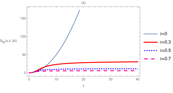
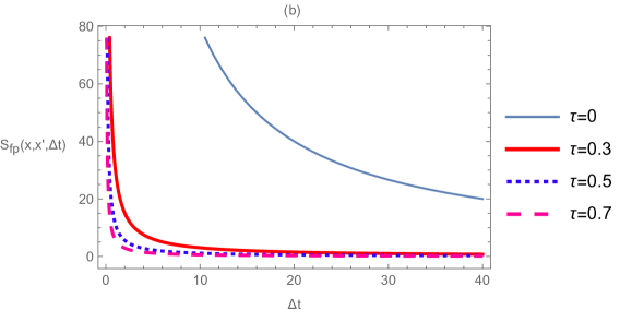
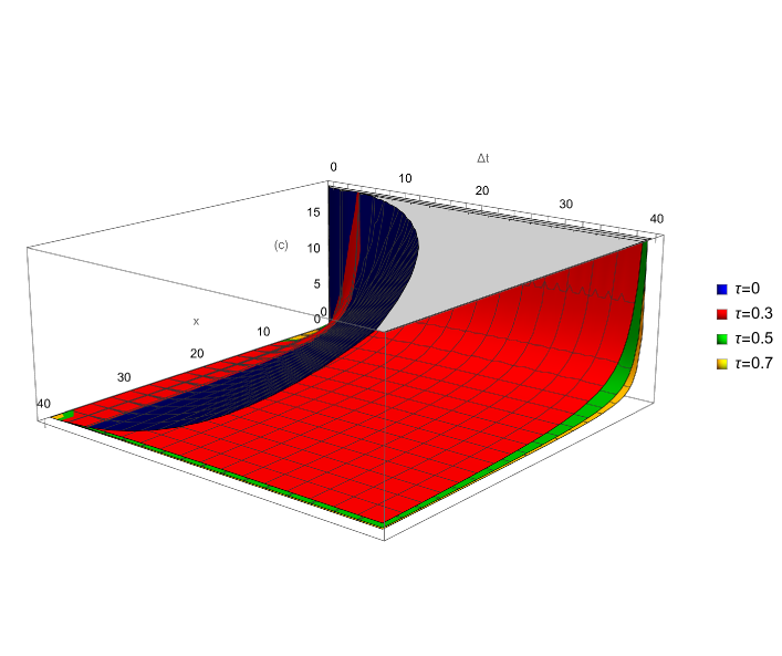
Figure 1: Classical action of a free particle (76) versus the position $x$ and the time $\Delta t$ for different values of $\tau$ with $m=1$.

The propagator for the Fourier transform and its inverse representions is given by

$$\mathcal{K}(\rho,\rho^{\prime},\Delta t) = \frac{1}{2\hbar\pi}\sqrt{\frac{m}{2\hbar\pi i\Delta t}}\int_{-\infty}^{+\infty}\frac{dx}{1-\tau x+\tau^{2}x^{2}}\int_{-\infty}^{+\infty}\frac{dx^{\prime}}{1-\tau x^{\prime}+\tau^{2}x^{\prime 2}}$$ (82)

$$\times e^{-i\frac{2}{\tau\hbar\sqrt{3}}\left[\rho\arctan\left(\frac{2\tau x-1}{\sqrt{3}}\right)-\rho^{\prime}\arctan\left(\frac{2\tau x^{\prime}-1}{\sqrt{3}}\right)\right]}$$

$$\times e^{i\frac{2m}{\hbar 3\tau^{2}\Delta t}\left[\arctan\left(\frac{2\tau x-1}{\sqrt{3}}\right)-\arctan\left(\frac{2\tau x^{\prime}-1}{\sqrt{3}}\right)\right]^{2}}.$$

The corresponding action is given by

$$\mathcal{S}_{fp}=S_{fp}-\frac{2}{\tau\sqrt{3}}\left[\rho\arctan\left(\frac{2\tau x-1}{\sqrt{3}}\right)-\rho^{\prime}\arctan\left(\frac{2\tau x^{\prime}-1}{\sqrt{3}}\right)\right].$$ (83)

3.3.2 A simple Harmonic oscillator

The simple harmonic oscillator problem is defined by the Hamiltonian

$$\hat{H}=\frac{\hat{P}^{2}}{2m}+\frac{1}{2}m\omega^{2}\hat{X}^{2}.$$ (84)

The propagator in position representation is given by

$$K_{ho}(x,x^{\prime},\Delta t) = \langle x|e^{-\frac{i}{\hbar}\left(\frac{\hat{P}^{2}}{2m}+\frac{1}{2}m\omega^{2}\hat{X}^{2}\right)\Delta t}|x^{\prime}\rangle$$ (85)

$$= \frac{1}{\tau\hbar\sqrt{3}}\langle x|e^{-\frac{i}{2\hbar}m\omega^{2}x^{\prime 2}\Delta t}\int_{-\infty}^{+\infty}d\rho e^{-\frac{i}{\hbar}\frac{\hat{P}^{2}}{2m}\Delta t}|\rho\rangle\langle\rho|x^{\prime}\rangle$$ (86)

$$= \int_{-\infty}^{+\infty}\frac{d\rho}{2\pi\hbar}$$ (88)

$$\times e^{\left(i\frac{2\rho}{\tau\hbar\sqrt{3}}\left[\arctan\left(\frac{2\tau x-1}{\sqrt{3}}\right)-\arctan\left(\frac{2\tau x^{\prime}-1}{\sqrt{3}}\right)\right]-\frac{i}{\hbar}\left(\frac{\rho^{2}}{2m}+\frac{1}{2}m\omega^{2}x^{\prime 2}\right)\Delta t\right)}.$$

Computing the Gaussian integral (88), we have

$$K_{ho}(x,x^{\prime},\Delta t)=\sqrt{\frac{m}{2\pi\hbar i\Delta t}}e^{i\frac{2m}{\hbar 3\tau^{2}\Delta t}\left[\arctan\left(\frac{2\tau x-1}{\sqrt{3}}\right)-\arctan\left(\frac{2\tau x^{\prime}-1}{\sqrt{3}}\right)\right]^{2}-\frac{i}{2\hbar}m\omega^{2}x^{\prime 2}\Delta t},$$ (89)

and the corresponding deformed classical action is given by

$$S_{ho}=\frac{2m}{3\tau^{2}\Delta t}\left[\arctan\left(\frac{2\tau x-1}{\sqrt{3}}\right)-\arctan\left(\frac{2\tau x^{\prime}-1}{\sqrt{3}}\right)\right]^{2}-\frac{1}{2}m\omega^{2}x^{\prime 2}\Delta t.$$ (90)

At the limit $\tau\rightarrow 0$, we recover the ordinary propagator and the classical action of the simple harmonic oscillator [21, 22]

$$\lim_{\tau\rightarrow 0}K_{ho}(x,x^{\prime},\Delta t) = K_{ho}^{0}(x,x^{\prime},\Delta t)=\sqrt{\frac{m}{2\pi\hbar i\Delta t}}e^{\frac{i}{\hbar}\left(\frac{m(x-x^{\prime})^{2}}{2\Delta t}-\frac{1}{2}m\omega^{2}x^{\prime 2}\Delta t\right)},$$ (91)

$$\lim_{\tau\rightarrow 0}S_{ho} = S_{ho}^{0}=\frac{m(x-x^{\prime})^{2}}{2\Delta t}-\frac{1}{2}m\omega^{2}x^{\prime 2}\Delta t=E_{m},$$ (92)

where $E_{m}$ is the mechanical energy of a simple harmonic mechanics. Like in the prior instance (93), It is simple to demonstrate that

$$K_{ho}(x,x^{\prime},\Delta t)\leq K_{ho}^{0}(x,x^{\prime},\Delta t)\implies S_{ho}\leq S_{ho}^{0}.$$ (93)

In more general case, we can see that the harmonic oscillator potential does not affect the motion of the deformed motion of the free particle such as

$$K_{ho}\approx K_{fp}\leq K_{fp}^{0}\approx K_{ho}^{0}\implies S_{ho}\approx S_{fp}\leq S_{fp}^{0}\approx S_{ho}^{0}.$$ (94)

The propagator in Fourier transform and its inverse representions is given by

$$\mathcal{K}(\rho,\rho^{\prime},\Delta t) = \frac{1}{2\pi}\sqrt{\frac{m}{2\pi\hbar i\Delta t}}\int_{-\infty}^{+\infty}\frac{dx}{1-\tau x+\tau^{2}x^{2}}\int_{-\infty}^{+\infty}\frac{dx^{\prime}}{1-\tau x^{\prime}+\tau^{2}x^{\prime 2}}$$ (97)

$$\times e^{-i\frac{2}{\tau\hbar\sqrt{3}}\left[\rho\arctan\left(\frac{2\tau x-1}{\sqrt{3}}\right)-\rho^{\prime}\arctan\left(\frac{2\tau x^{\prime}-1}{\sqrt{3}}\right)\right]}$$

$$\times e^{i\frac{2m}{\hbar 3\tau^{2}\Delta t}\left[\arctan\left(\frac{2\tau x-1}{\sqrt{3}}\right)-\arctan\left(\frac{2\tau x^{\prime}-1}{\sqrt{3}}\right)\right]^{2}-\frac{i}{2\hbar}m\omega^{2}x^{\prime 2}\Delta t},$$

and its action is given by

$$\mathcal{S}_{ho} = S_{ho}-\frac{2}{\tau\sqrt{3}}\left[\rho\arctan\left(\frac{2\tau x-1}{\sqrt{3}}\right)-\rho^{\prime}\arctan\left(\frac{2\tau x^{\prime}-1}{\sqrt{3}}\right)\right].$$ (98)

4 Conclusion

We have constructed path integrals in Euclidean position representation and in Fourier transform and its inverse representations within a position-deformed Heisenberg algebra. We have derived from these path integrals the propagators and the corresponding classical actions. The classical equations of motion are obtained by the principle of least action. The Hamiltonians of a free particle and a simple harmonic oscillator are used as examples to compute the propagators and the actions in position representation and in Fourier transform and inverse representations. We have shown through these that the propagators and the actions of these systems in position space representation are properly bounded by the well-known results in the $\tau\rightarrow 0$ limit. These mathematical results have been confirmed by the numerical investigations of the classical action of these systems. We have observed that simultaneous variation of the action in time and in position rapidily decreases as one increases the parameter of quantum gravity $\tau$. This suggests that quantum gravity in this space bends particle pathways, allowing them to travel fast from one point to the next. The propagators for Fourier transform and its inverse representations for both systems are given as integral expressions and we have deduced the corresponding actions.

In this work, we have constructed path integrals in the deformed Heisenberg algebra from the Schrödinger equation. One can extend this work on the stochastic path integrals using the Fokker-Planck equation [23, 24, 25, 26] or to derive the Black–Scholes pricing kernel from the Black–Scholes equation [27].

References

• [1] L. Lawson, Position-dependent mass in strong quantum gravitational background fields, J. Phys. A: Math. Theor. 55, 105303 (2022)
• [2] A. Kempf, G. Mangano and R. Mann, Hilbert space representation of the minitial length uncertainty relation, Phys. Rev. D 52, 1108 (1995)
• [3] A. Kempf, G. Mangano, Minimal length uncertainty relation and ultraviolet regularization, Phys. Rev. D. 55 7909-7920 (1997).
• [4] Y. Sabri and K. Nouicer, Phase transitions of a GUP-corrected Schwarzschild black hole within isothermal cavities, Class. Quant. Grav. 29 , 215015 (2012)
• [5] A. Ali, S. Das and E. Vagenas, Discreteness of space from the generalized uncertainty principle, Phys. Lett.B 678, 497 (2009)
• [6] S. Das, E. Vagenas and A. Ali, Discreteness of space from GUP II: Relativistic wave equations, Phys. Lett. B, 690, 407 (2010)
• [7] Pouria Pedram, A higher order GUP with minimal length uncertainty and maximal momentum, Physics Letters B 714, 317-323 (2012)
• [8] Pouria Pedram, A higher order GUP with minimal length uncertainty and maximal momentum II, Physics Letters B 718, 638–645 (2012)
• [9] F. Scardiglia and R. Casadio, Gravitational tests of the Generalized Uncertainty Principle, Eur. Phys. J. C 75, 425 (2015).
• [10] K. Nozari and A. Etemadi, Minimal length, maximal momentum and Hilbert space representation of quantum mechanics, Phys. Rev. D 85, 104029 (2012)
• [11] A. Tawfik and A. Diab, A review of the generalized uncertainty principle, Rep. Prog. Phys. 78, 126001 (2015)
• [12] L. Lawson, L. Gouba and G. Avossevou, Two-dimensional noncommutative gravitational quantum well, J. Phys A: Math. Theor 50, 475202 (2017)
• [13] W. Sang Chung and H. Hassanabadi, A new higher order GUP: one dimensional quantum system, Eur. Phys. J.C 79, 213 (2019)
• [14] L. Lawson, Minimal and maximal lengths from position-dependent noncommutativity, J. Phys. A: Math. Theor. 53, 115303 (2020)
• [15] R. Bernardo and J. Esguerra, Euclidean path integral formalism in deformed space with minimum measurable length, J. Math. Phys. 58, 042103 (2017)
• [16] S. Bhattacharyya and S. Gangopadhyay, Path-integral action in the generalized uncertainty principle framework, Phys. Rev. D 104, 026003 (2021)
• [17] K. Nouicer, Coulomb potential in one dimension with minimal length: A path integral approach, J. Math. Phys. 48, 112104 (2007)
• [18] P. Valtancoli, Path integral and noncommutative Poisson brackets, J. Math. Phys. 56, 063501 (2015)
• [19] I. Gradshteyn and M. Ryzhik, Table of Integrals, Series, and Products, 8th ed. (Academic Press, San Diego, California, USA, 2015).
• [20] S. Das and S. Pramanik, Path integral for nonrelativistic generalized uncertainty principle corrected Hamiltonian, Phys. Rev. D 86, 085004 (2012)
• [21] H. Klein, Path Integral in Quantum Statistics and Polymer Physics, World Scientific Singapore, 1990
• [22] D. C. Khandekar, S. V. Lawande, and K. V. Bhagwat, Path Integrals Methods and Their Application, World Scientific Singapore,1993
• [23] P. Bressloff, Coherent spin states and stochastic hybrid path integrals, J. Stat. Mech. (2021) 043207
• [24] P. Bressloff, Construction of stochastic hybrid path integrals using operator methods, J. Phys. A: Math. Theor. 54, 185001 (2021)
• [25] J. Vastola and W. Holmes, Stochastic path integrals can be derived like quantum mechanical path integrals, arXiv:1909.12990 [cond-mat.stat-mech]
• [26] B. da Costa, I. Gomez, and E. Borges, Deformed Fokker-Planck equation: Inhomogeneous medium with a position-dependent mass, Phys. Rev. E 102, 062105 (2020)
• [27] B. Baaquie, Quantum Finance, Path Integral and Hamiltonians for options and interest rates, Cambridge University Press The Edinburgh Building, Cambridge CB2 8RU, UK